Insights and Approaches for Mapping Soil Organic Carbon as a

Dynamic Soil Property

Mark H. Stolt, Patrick J. Drohan, and Matthew J. Richardson

Soil Science Society of America Journal (2010)

Site Locations

17 sites, ranging in age from 25 to 86 years.

1954

1997

•Field and forest having same soil type comprise paired site •Sample multiple locations within field and forest •Core trees to determine age and measure SOC •Difference between field and forest used to calculate rate of C sequestration

Paired Sites:

Anderson Land Cover Level I O A B C

Upper Meter

Percent of Upper Meter

Pool in O and A Horizons

Numeric Phase Value

──────── Mg ha-1 ──────────── % (Mg ha-1)

Agricultural 0 55 35 15 103 53 55 (Moderate)

Forest 32 70 40 17 157 65 102 (High)

Average SOC by horizon and for the upper meter by Anderson Land Cover Class

Add a phase component to the Soil Survey for SOC pools Focus on the O and A horizon For example: MmB in the soil survey in agriculture would be changed to MmBM

Assessing the Effects of Land Use Change

on Riparian Zone Soils in Southern

New England Matthew C. Ricker

Mark H. Stolt

Ecological Applications 2012

Matt Ricker

• Important links between upland and aquatic systems

• Provide multiple environmental

and ecosystem functions • Form as a result of episodic alluvial

deposition • Land use change may result in impacts to riparian soil functions

Buried horizon (Ab) RIPARIAN ZONES

Develop Multi-Proxy Indices of Land Use Change for Riparian Soils

Objectives

1. Establish stratigraphic indices of watershed land use change using a multi-proxy approach

2. Utilize these indices to establish time frames of alluvial deposition 3. Relate riparian sedimentation and carbon sequestration rates to land use

Diatomaceous Earth

SEM Image 500x Magnification

Methods • 18 representative headwater

watershed riparian sites selected – Hydric soils (Inceptisols, Entisols)

• Formed in alluvium over outwash

• Raypol, Rumney, Scarboro, and Walpole series

• Varied watershed land use – Urban, agricultural, mixed use, forested

• Soil pits dug to 1 m or greater – Soils described in field

– Bulk density

– PSD

– Heavy metals

– Pollen samples by horizon

– Soil organic carbon (SOC)

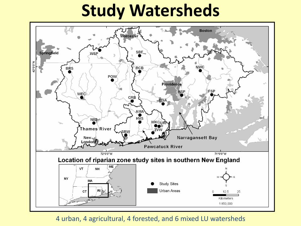
Study Watersheds

4 urban, 4 agricultural, 4 forested, and 6 mixed LU watersheds

General Land Use Periods and Associated Indices • Constrain riparian soil horizons into three

major distinct land use periods

• Pre-colonial period (17,000 YBP–1650 AD)

• Colonial (agrarian) period (1650-1900 AD)

– Rise and/or peak ragweed and other non-arboreal pollen types

– Supported by twelve 14C dates • Rise in ragweed dated to 1780±40 AD

• Peak ragweed dated to 1850±50 AD

• Modern industrial/urbanization period (1900 AD-present)

– Increased coarse materials (sand, gravels)

– Presence of human artifacts

– Rise and peak pollutant metals (Pb) • Supported by 210Pb cores

Many sand lenses (A/Cg)

• Particle size distribution – Coarser deposits as watersheds

undergo extensive LU change

• Buried horizons (i.e. Ab) • Combination horizons (i.e. A/C)

– Indicative of short term stability

• Human artifacts (i.e. Cu horizon) – Indicative of colonial-urban time

periods

• Pollutant metals – Pb, Cu, Zn, Cd, As above

background levels; on average 3 to 6 times higher in surface horizons

Indices of Land Use Change: Soil Morphology and Pollutant Metals

Examples of Riparian “Artifacts” (One Person’s Garbage is Another’s Stratigraphic Marker…)

A: Glass B: Plastic C: Cloth D: Asphalt E: Brick F: Styrofoam G: Shingle 50 cm 15 cm 20 cm 30 cm 50 cm 15 cm 40 cm

Pollutant Metals Indices of Anthropogenic Activities

(1900-present)

Concentration of pollutant metals in riparian zone soil horizons

a a

b

y y

z

050

100150200250300

Upper Most Horizon(n=18)

Upper Most MineralHorizon (n=18)

Glacial ParentMaterials (n=31)

(mg

kg-1)

Pb Total Pb, Zn, Cu, Cd, AsMeans with different letters are significantly different (α=0.05)

Metals concentrated near soil surface, likely anthropogenic origins: 1900-present fossil fuel combustion, especially leaded gasoline

• Past land uses affected the vegetation of the region – Impacts evident in pollen record

– Pollen stratigraphy can be used to reconstruct land use

• Pollen indicators, specifically: – ragweed (Ambrosia taxa, family Asteraceae)

– grasses (Poaceae)

– have been used to date peak land use disturbance in many depositional environments (lakes and ponds)

Grass pollen (monoporate)

Ragweed pollen (tricolporate, spines)

Indices of Land Use Change: Preserved Pollen (Colonial Period)

• Moderate to abundant pollen was preserved in subsurface horizons • Range 300 to >60,000 pollen grains per gram of soil • Pollen was preserved in horizons dated to >11,000 YBP • 88% riparian soils contained preserved pollen • 71% riparian soils contained enough pollen for land use stratigraphy

Example Pollen Diagrams

-110-100-90-80-70-60-50-40-30-20-10

00 10 20 30 40 50

% Pollen

Dep

th (c

m)

Non-arboreal Ragweed Alder

-60

-50

-40

-30

-20

-10

00 10 20 30 40 50

% Pollen

Dep

th (c

m)

Non-arboreal Ragweed AlderAMA-RI URI-RI 1230 45 AD

1770 40 AD

1870 67 AD

1770 41 AD

Mean Proportion (%) Riparian Sediment and SOC from Major Land Use Periods

16 (69)30 (60)

51 (45)45 (49)

33 (76)25 (80)

0%

25%

50%

75%

100%

% Sediment % SOC

Pre-Colonial Colonial Modern

70% 84%

a

b

ab a

b

a * **

* p-value < 0.01 ** p-value < 0.0001

n = (24)

Average net sediment and SOC distribution by land use period

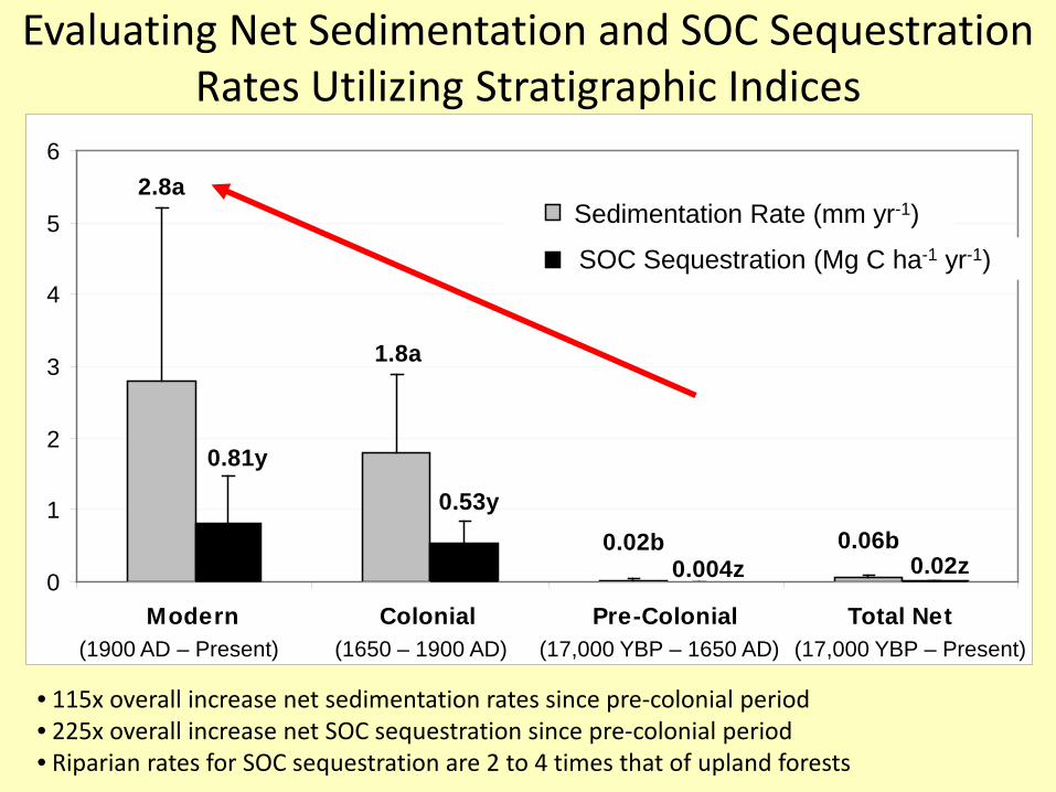
Evaluating Net Sedimentation and SOC Sequestration Rates Utilizing Stratigraphic Indices

2.8a

1.8a

0.02b 0.06b

0.81y

0.53y

0.004z 0.02z0

1

2

3

4

5

6

Modern Colonial Pre-Colonial Total Net

Accretion Rate

SOC SeqestrationSOC Sequestration (Mg C ha-1 yr-1)

Sedimentation Rate (mm yr-1)

(1900 AD – Present) (1650 – 1900 AD) (17,000 YBP – 1650 AD) (17,000 YBP – Present)

• 115x overall increase net sedimentation rates since pre-colonial period • 225x overall increase net SOC sequestration since pre-colonial period • Riparian rates for SOC sequestration are 2 to 4 times that of upland forests

Sedimentation and SOC Sequestration: What is the relationship?

y = 0.2378x + 0.0834R2 = 0.70

0.0

0.5

1.0

1.5

2.0

2.5

3.0

0 2 4 6 8 10Sedimentation Rate (mm yr-1)

SOC

Seq

uest

ratio

n (M

g C

ha-1

yr-1

)

Pre-ColonialColonialModern

• Suggests sedimentation and SOC sequestration are related. • Exact driver of this relationship is unclear (burial, C influx, additional surface area?).

Conclusions • Soil morphology, pollutant

metals, and pollen stratigraphy can be used to successfully date riparian soil deposition

• Land use change has had significant impacts on riparian zone sedimentation and C sequestration – Riparian zones acting as large

sinks for sediment and C – Riparian SOC sequestration and

sedimentation may be linked processes

Ab horizon

1770 AD 40

Are riparian zones “hot spots” for SOC at

watershed-scale Methods --29 representative riparian soil pedons

were examined, (Blazejewski, 2003; Donohue, 2007; Ricker, 2010)

--Soils sampled by horizon to 1 m - Bulk density - SOC - Calculated SOC pools at landscape

scale (Mg C ha-1) --Riparian SOC pools compared to

published data (Davis et al., 2004) Watershed-scale analysis done in GIS

SOC Pools Across the Landscape

110a136a

187b

246c

586d

0

100

200

300

400

500

600

700

ED WD PD Riparian VPD(Organic)

SOC

Poo

l (M

g C

ha-1

)

0

* From (Davis et al., 2004)

*

*

* *

Means with different letters are sig. dif. (α = 0.05) Error bars = 1 SD

Uplands

Wetlands

• Mean riparian SOC pool was 246 Mg C ha-1

• SOC pools (to 1 m depth) in riparian zone more than all other mineral soils evaluated by Davis et al. (2004) • Only Histosols contained more SOC to 1 m

Spatial Distribution of SOC in Riparian Soils

53 (64)

47 (43)

0%

25%

50%

75%

100%

Riparian Zone SOCDistribution (n=29)

Prop

ortio

n To

tal S

OC

Lower 70 cm Upper 30 cm

• 53% SOC below 30 cm depth • By comparison: • ED - 30% • WD - 30% • PD - 45% • VPD - 75%

• In addition: • 52% of riparian soils studied had buried SOC rich horizons below 1 m • Suggests deep burial of SOC is important in riparian landscapes

CV (%) in parentheses

Factors Affecting Riparian SOC Pools

Urban Riparian Soil Norwich, CT

• Many factors tested, none significant • Differences in SOC with differences in soil morphology

• Soils with buried surface horizons contained significantly more SOC • Suggests riparian soils with high sedimentation contain more SOC

p = 0.01

188 b

277 a

050

100150200250300

With Buried SurfaceHorizons (n=19)

Without Buried SurfaceHorizons (n=10)

SOC

to 1

m (M

g C

ha-1

)

Riparian SOC Pools at a Watershed-scale

• On average, riparian zones comprised 8% of the total watershed area • Contained as much as 20% of the total watershed SOC • Riparian zones occupy small portion of the landscape, but represent large sink for SOC at a watershed-scale

Example GIS Map

M. H. Stolt and M. C. Rabenhorst University of Rhode Island

University of Maryland

Field Estimations of Soil Organic Carbon

Field Estimations of Soil Properties

• Redoximorphic Features

• Soil Texture

• Soil Organic Carbon – Mineral soil materials

– Mucky modified soil materials

– Organic soil materials

Field Indicators of Hydric Soils

• Thirteen of the approved field indicators of hydric soils (A1, A2, A3, A5, A6, A7, A8, A9, A10, S1, S2, S3, F1) require the recognition of organic or mucky modified materials as part of their definition.

We Asked:

• How well can this be done?

Methodology

• Two parallel studies • One utilized members and participants in the

Mid-Atlantic Hydric Soils committee • The second utilized members of the New England

Hydric Soils Committee • These groups were selected because they mainly

included experienced soil and wetland scientists who had some experience in making distinctions among mineral, mucky mineral, and organic soil materials.

0

5

10

15

20

25

0 20 40 60 80 100

Perc

ent O

C

Percent Clay

Mucky Modified

Mineral

Organic

USDA-NRCS. 2010. Field Indicators of Hydric Soils in the United States, Version 7.0. USDA, NRCS, in cooperation with the National Technical Committee for Hydric Soils.

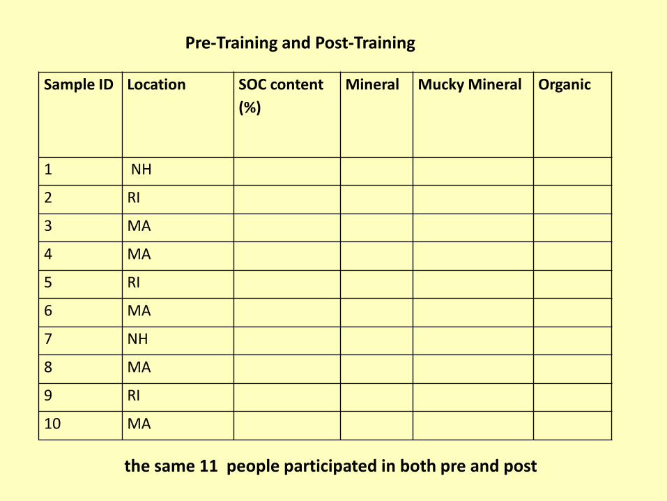
Sample ID Location SOC content (%)

Mineral Mucky Mineral Organic

1 NH

2 RI

3 MA

4 MA

5 RI

6 MA

7 NH

8 MA

9 RI

10 MA

Pre-Training and Post-Training

the same 11 people participated in both pre and post

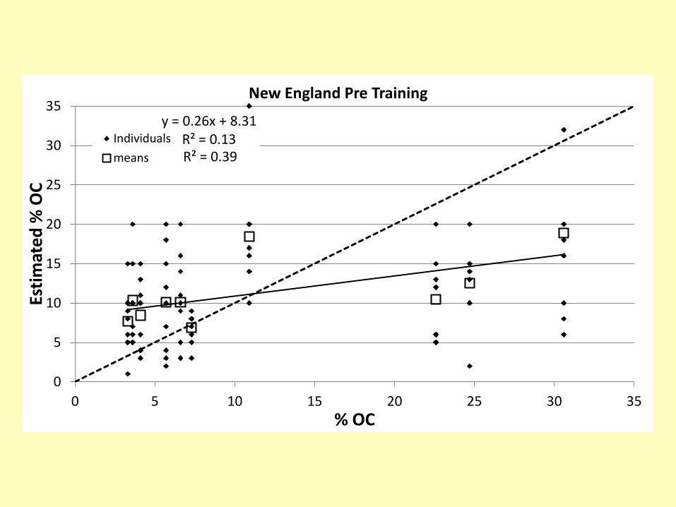
y = 0.26x + 8.31R² = 0.13R² = 0.39

0

5

10

15

20

25

30

35

0 5 10 15 20 25 30 35

Esti

mat

ed %

OC

% OC

New England Pre Training

Individuals

means

y = 0.46x + 4.70R² = 0.50

R² = 0.89

0

5

10

15

20

25

30

35

0 5 10 15 20 25 30 35

Esti

mat

ed %

OC

% OC

New England Post Training

Individuals

means

p < 0.001

Participant A B C D E F G H I J K

Average correct

(%)

Pre-training Correct (%) 60 50 60 30 30 40 40 50 30 20 40 41% After training Correct (%) 70 80 50 50 60 100 50 70 70 70 80 68% Individual Improvement (%) 10 30 -10 20 30 60 10 20 40 50 40 27%

New England Class Assignment Results

y = 0.58x + 2.06R² = 0.23R² = 0.81

0

5

10

15

20

25

30

0 5 10 15 20 25 30

Esti

mat

ed %

OC

% OC

Mid-Atl Pre Training

IndividualsMeans

p < 0.001

y = 0.57x + 3.80R² = 0.48R² = 0.70

0

5

10

15

20

25

30

0 5 10 15 20 25 30

Esti

mat

ed %

OC

% OC

Mid-Atl Post Training

IndividualsMeans

p < 0.001

Participant A B C D E F G H I average correct

Pretraining Correct 45% 55% 36% 45% 73% 64% 64% 45% 73% 56%

Aftertraining Correct 73% 55% 45% 55% 73% 91% 82% 64% 82% 69%

Individual Improvement 27% 0% 9% 9% 0% 27% 18% 18% 9% 13%

Mid-Atlantic Class Assignment Results

0%

10%

20%

30%

40%

50%

60%

70%

80%

Mid-Atlantic New England

Corr

ect P

lace

men

t

Set 1

Set 2

a

b

c c

Placement into classes: mineral, mucky modified, organic

Summary

• Not easy to estimate SOC and determine between mucky modified and mineral or organic soil materials

• Without training New England folks could only assign the correct class on average 41% of the time.

• Training improved our ability to assign the correct class (68%). This was essentially the same amount as the Mid-Atlantic committee got correct after training (69%)

• In general we over-estimate SOC in mineral soil materials and under-estimate SOC in organic soil materials.

Method Fibric Hemic Sapric

Field 0 3 82

Lab

Determination of soil organic soil material (SOM) type. Field is based on visual rubbed fiber content. Lab is based in standard lab rubbed fiber approach and sodium-pyrophosphate color. n = 85.

Method Fibric Hemic Sapric

Field 0 3 82

Lab 8 49 28

Determination of soil organic soil material (SOM) type. Field is based on visual rubbed fiber content. Lab is based in standard lab rubbed fiber approach and sodium-pyrophosphate color. n = 85.

Mesic-Spodic Hydric Soil Indicator: Development and Testing We investigated 33 pedons for which we had 2 to 4 years of surface hydrology data for six sites. Most of the wetter soils had spodic morphology. Based on the hydrology, 25 pedons were identified as hydric. Five of the pedons met both the NE regional and national indicators. Two of the hydric pedons met the NE regional indicators but failed to meet the national indicator. Eight hydric pedons met national indicators but did not meet New England regional indicators, and 10 hydric pedons did not meet either the national nor regional indicator. Thus, 40% of the hydric soils reviewed did not meet any indicator and suggested the need for the development of an effective indicator for hydric spodic soils. Thus, our goal was to develop and test such an indicator.

Cooper Cedar Woods (CCW) Pit #1 NH Soil Judging Contest 2005. Likely an Alaquod or Duraquod.

Plates from Bhsm. Note the mottled appearance that suggests Fe concentrations

Bhsm. Plates and mottled appearance.

Bhsm over bedrock on last stop during 2005 Maine tour. Note Fe concentrations.

Bhsm in NH formed in outwash (CCW Pit #1). No concentrations observed.

Bw and Bhsm for comparison.

Samples photographed after heating to 550 degrees C in muffle furnace to remove organic matter.

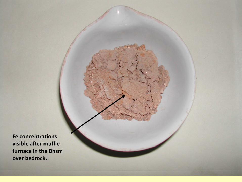
Fe concentrations visible after muffle furnace in the Bhsm over bedrock.

Roque Bluffs Maine 2005 NEHSTC Fall Tour

E Horizon Bhs Horizon Bs Horizon Pit #4

Pit #2

Bw horizon and Bhsm horizon

TA6. Mesic Spodic. For testing in MLRAs 144A and 145 of LRR R and MLRA 149B of LRR S. A layer 5 cm (2 inches) or more thick, starting within 15 cm (6 inches) of the mineral soil surface, that has value of 3 or less and chroma of 2 or less and is underlain by either: a. A layer(s) 8 cm (3 inches) or more thick occurring within 30

cm (12 inches) of the mineral soil surface, having value and chroma of 3 or less, and showing evidence of spodic development; or

b. A layer(s) 5 cm (2 inches) or more thick occurring within 30 cm (12 inches) of the mineral soil surface, having value of 4 or more and chroma of 2 or less, and directly underlain by a layer(s) 8 cm (3 inches) or more thick having value and chroma of 3 or less and showing evidence of spodic development.

Dark surface at least 2” thick and;

1) Layer at least 3” thick starting within 12” of soil surface that is 3/3 or darker and shows evidence of spodic morphology; or

2) A layer 2” or more thick occurring within 12” of the mineral soil surface, having value of 4 or more and chroma of 2 or less, and directly underlain by a layer 3” or more thick having value and chroma of 3 or less and showing evidence of spodic development.

• There are 4 monitoring sites:

•Two in Rhode Island

•Two in Massachusetts • Year 1 data

• all met the indicator, • showed reduction on IRIS tubes, and • met wetland hydrology