
InsCLR: Improving Instance Retrieval with Self-Supervision
12
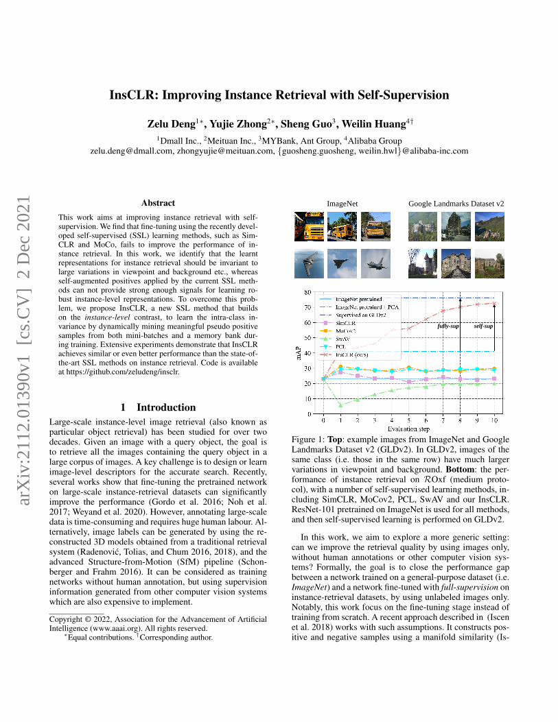
InsCLR: Improving Instance Retrieval with Self-Supervision Zelu Deng 1* , Yujie Zhong 2* , Sheng Guo 3 , Weilin Huang 4† 1 Dmall Inc., 2 Meituan Inc., 3 MYBank, Ant Group, 4 Alibaba Group [email protected], [email protected], {guosheng.guosheng, weilin.hwl}@alibaba-inc.com Abstract This work aims at improving instance retrieval with self- supervision. We find that fine-tuning using the recently devel- oped self-supervised (SSL) learning methods, such as Sim- CLR and MoCo, fails to improve the performance of in- stance retrieval. In this work, we identify that the learnt representations for instance retrieval should be invariant to large variations in viewpoint and background etc., whereas self-augmented positives applied by the current SSL meth- ods can not provide strong enough signals for learning ro- bust instance-level representations. To overcome this prob- lem, we propose InsCLR, a new SSL method that builds on the instance-level contrast, to learn the intra-class in- variance by dynamically mining meaningful pseudo positive samples from both mini-batches and a memory bank dur- ing training. Extensive experiments demonstrate that InsCLR achieves similar or even better performance than the state-of- the-art SSL methods on instance retrieval. Code is available at https://github.com/zeludeng/insclr. 1 Introduction Large-scale instance-level image retrieval (also known as particular object retrieval) has been studied for over two decades. Given an image with a query object, the goal is to retrieve all the images containing the query object in a large corpus of images. A key challenge is to design or learn image-level descriptors for the accurate search. Recently, several works show that fine-tuning the pretrained network on large-scale instance-retrieval datasets can significantly improve the performance (Gordo et al. 2016; Noh et al. 2017; Weyand et al. 2020). However, annotating large-scale data is time-consuming and requires huge human labour. Al- ternatively, image labels can be generated by using the re- constructed 3D models obtained from a traditional retrieval system (Radenovi´ c, Tolias, and Chum 2016, 2018), and the advanced Structure-from-Motion (SfM) pipeline (Schon- berger and Frahm 2016). It can be considered as training networks without human annotation, but using supervision information generated from other computer vision systems which are also expensive to implement. Copyright © 2022, Association for the Advancement of Artificial Intelligence (www.aaai.org). All rights reserved. * Equal contributions. † Corresponding author. Google Landmarks Dataset v2 ImageNet self-sup fully-sup Figure 1: Top: example images from ImageNet and Google Landmarks Dataset v2 (GLDv2). In GLDv2, images of the same class (i.e. those in the same row) have much larger variations in viewpoint and background. Bottom: the per- formance of instance retrieval on ROxf (medium proto- col), with a number of self-supervised learning methods, in- cluding SimCLR, MoCov2, PCL, SwAV and our InsCLR. ResNet-101 pretrained on ImageNet is used for all methods, and then self-supervised learning is performed on GLDv2. In this work, we aim to explore a more generic setting: can we improve the retrieval quality by using images only, without human annotations or other computer vision sys- tems? Formally, the goal is to close the performance gap between a network trained on a general-purpose dataset (i.e. ImageNet) and a network fine-tuned with full-supervision on instance-retrieval datasets, by using unlabeled images only. Notably, this work focus on the fine-tuning stage instead of training from scratch. A recent approach described in (Iscen et al. 2018) works with such assumptions. It constructs pos- itive and negative samples using a manifold similarity (Is- arXiv:2112.01390v1 [cs.CV] 2 Dec 2021
Transcript of InsCLR: Improving Instance Retrieval with Self-Supervision
InsCLR: Improving Instance Retrieval with Self-Supervision
Zelu Deng1∗, Yujie Zhong2∗, Sheng Guo3, Weilin Huang4†
1Dmall Inc., 2Meituan Inc., 3MYBank, Ant Group, 4Alibaba [email protected], [email protected], {guosheng.guosheng, weilin.hwl}@alibaba-inc.com
AbstractThis work aims at improving instance retrieval with self-supervision. We find that fine-tuning using the recently devel-oped self-supervised (SSL) learning methods, such as Sim-CLR and MoCo, fails to improve the performance of in-stance retrieval. In this work, we identify that the learntrepresentations for instance retrieval should be invariant tolarge variations in viewpoint and background etc., whereasself-augmented positives applied by the current SSL meth-ods can not provide strong enough signals for learning ro-bust instance-level representations. To overcome this prob-lem, we propose InsCLR, a new SSL method that buildson the instance-level contrast, to learn the intra-class in-variance by dynamically mining meaningful pseudo positivesamples from both mini-batches and a memory bank dur-ing training. Extensive experiments demonstrate that InsCLRachieves similar or even better performance than the state-of-the-art SSL methods on instance retrieval. Code is availableat https://github.com/zeludeng/insclr.
1 IntroductionLarge-scale instance-level image retrieval (also known asparticular object retrieval) has been studied for over twodecades. Given an image with a query object, the goal isto retrieve all the images containing the query object in alarge corpus of images. A key challenge is to design or learnimage-level descriptors for the accurate search. Recently,several works show that fine-tuning the pretrained networkon large-scale instance-retrieval datasets can significantlyimprove the performance (Gordo et al. 2016; Noh et al.2017; Weyand et al. 2020). However, annotating large-scaledata is time-consuming and requires huge human labour. Al-ternatively, image labels can be generated by using the re-constructed 3D models obtained from a traditional retrievalsystem (Radenovic, Tolias, and Chum 2016, 2018), and theadvanced Structure-from-Motion (SfM) pipeline (Schon-berger and Frahm 2016). It can be considered as trainingnetworks without human annotation, but using supervisioninformation generated from other computer vision systemswhich are also expensive to implement.
Copyright © 2022, Association for the Advancement of ArtificialIntelligence (www.aaai.org). All rights reserved.
∗Equal contributions. †Corresponding author.
Google Landmarks Dataset v2ImageNet
self-supfully-sup
Figure 1: Top: example images from ImageNet and GoogleLandmarks Dataset v2 (GLDv2). In GLDv2, images of thesame class (i.e. those in the same row) have much largervariations in viewpoint and background. Bottom: the per-formance of instance retrieval on ROxf (medium proto-col), with a number of self-supervised learning methods, in-cluding SimCLR, MoCov2, PCL, SwAV and our InsCLR.ResNet-101 pretrained on ImageNet is used for all methods,and then self-supervised learning is performed on GLDv2.
In this work, we aim to explore a more generic setting:can we improve the retrieval quality by using images only,without human annotations or other computer vision sys-tems? Formally, the goal is to close the performance gapbetween a network trained on a general-purpose dataset (i.e.ImageNet) and a network fine-tuned with full-supervision oninstance-retrieval datasets, by using unlabeled images only.Notably, this work focus on the fine-tuning stage instead oftraining from scratch. A recent approach described in (Iscenet al. 2018) works with such assumptions. It constructs pos-itive and negative samples using a manifold similarity (Is-
arX
iv:2
112.
0139
0v1
[cs
.CV
] 2
Dec
202
1

cen et al. 2017) computed from a similarity graph which isbuilt on Euclidean distance. However, it focuses on design-ing an offline preprocessing of the images to generate thecorresponding image labels, and the training procedure re-mains the same as the standard supervised training. In thiswork, we go beyond such offline preprocessing, and pro-vide a more dynamic solution that generates self-supervisedlearning signals in an online manner during training, withminimal offline computation.
Recent self-supervised learning (SSL) methods, such asMoCo (He et al. 2020) and SimCLR (Chen et al. 2020a),train networks by learning instance discrimination betweenself-image (or self-augmented image) and other images.However, for the task considered in this work, we find thatsimply applying these state-of-the-art SSL methods to learnimage-level representations for instance retrieval is far fromideal. As Figure 1 shows, performing self-supervised learn-ing with SimCLR or MoCov2 (Chen et al. 2020b) withan ImageNet-pretrained network on the recently releasedGoogle Landmarks Dataset v2 (Weyand et al. 2020) (with-out using ground-truth labels) can not obtain the expectedperformance on the public benchmark for instance retrieval:revisited Oxford (Radenovic et al. 2018).
As Figure 1 (top) shows, different from ImageNet, objectsin instance retrieval may have large variance in viewpoint,background clutter, occlusion and illumination conditionsetc.. Therefore, an important capability for instance retrievalis to learn strong object representations that are robust to thelarge intra-class variation, and to focus on discriminating ob-ject instances rather than images. However, existing image-level SSL methods (such as MoCov2 and SimCLR) can notfully explore the intra-class information which is particu-larly useful to instance retrieval in datasets like GLDv2.
Consequently, we introduce an instance-level SSLmethod that learns to capture the abovementioned proper-ties from instance-retrieval datasets. The proposed methodexplores contrastive learning signals explicitly from intra-class pairs by mining cross-image pseudo positives fromboth the mini-batches and a memory bank along the train-ing. It encourages the model to pull the images of the sameclass but having different viewpoints or backgrounds closerin the feature space. The mined positives provide much moremeaningful learning signals than the self-augmented imagepairs, particularly on learning robust intra-class represen-tations. The proposed method is code-named InsCLR. Wemake the following contributions:
– We identify the limitation of state-of-the-art image-levelSSL methods such as MoCov2 and SimCLR, and proposeInsCLR for instance-level SSL which is able to learn stronginstance representations robust to large intra-class variance.
– To build meaningful instance-level contrastive infor-mation, we propose new algorithms to dynamically minepseudo positives from both mini-batches and the memorybank in the contrastive learning framework.
– Extensive experiments across three public benchmarks(revisited Oxford, Paris and INSTRE) demonstrate that theproposed InsCLR surpasses all other self-supervised meth-ods, and even outperforms many recent supervised meth-ods. In particular, as Figure 1 shows, our InsCLR achieves
73.1 mAP on the revisited Oxford (medium), significantlyclosing the gap between the unsupervised fine-tuning andthe best-performing supervised counterpart (Weyand et al.2020) (76.2 mAP) on instance retrieval.
2 Related WorkImage representations for instance-level image retrieval.In image retrieval, representing images with image-level(i.e. global) features is particularly favoured in practicedue to its run-time efficiency. In the era of deep learn-ing, global features can be generated by aggregating CNNsfeatures (Babenko and Lempitsky 2015; Tolias, Sicre, andJegou 2015; Arandjelovic et al. 2016; Gordo et al. 2016;Radenovic, Tolias, and Chum 2016; Tolias, Avrithis, andJegou 2016; Noh et al. 2017; Radenovic, Tolias, and Chum2018). Apart from global features, local features are alsoused to perform spatial verification (Philbin et al. 2007; Nohet al. 2017; Cao, Araujo, and Sim 2020), which incorporatesthe geometric information of objects and results in a morereliable matching. In this work, we focus on learning globalimage descriptors with self-supervision due to its simplicity,and leave local descriptors for future work.Self-supervised representation learning. Recently,prominent performance in image classification is achievedby contrastive learning (Oord, Li, and Vinyals 2018; Heet al. 2020; Chen et al. 2020a,b; Caron et al. 2020). Inparticular, MoCo (He et al. 2020; Chen et al. 2020b),SimCLR (Chen et al. 2020a) and SwAV (Caron et al. 2020)further reduce the performance gap between self-supervisednetworks and fully-supervised networks. Different fromMoCo and SimCLR that learn by the image discrimination,SCAN (Van Gansbeke et al. 2020) and InterCLR (Xie et al.2020) reveal that more important semantic information canbe explored across images. Recent works, such as PCL (Liet al. 2020) and SwAV (Caron et al. 2020), were developedto learn intra-class information implicitly by assigningsimilar images to same prototypes/clusters. In this work, weshow that the intra-class information can be better exploredby explicitly finding cross-image positive pairs with apairwise learning paradigm.Feature memory bank. In contrastive learning frame-work, memory banks can be used in both supervised (Liet al. 2019; Wang et al. 2020) and unsupervised learning (Heet al. 2020; Chen et al. 2020b) with different motivations.Different from them, we propose to mine both positive andnegative samples in the memory for unsupervised learning,which has never been explored before.
3 The proposed InsCLRIn this section, we present details of the proposed InsCLRwhich is able to learn strong image representations for in-stance retrieval by mining pseudo positives and negatives ina self-supervised manner. We start from an overview of themethod (Section 3.1), including a formal definition of thetask, the network architecture and the setup for training sam-ples. Then, we describe details of mining positives in mini-batches (Section 3.2) and the memory bank (Section 3.3).The training loss is defined in Section 3.4.
w/o DAAnchor Neighbours
A training tuple in mini-batch
Candidate pool
BackboneSpatial
poolingEmbedding
Memory bank
w/ DA
update
Memory bank
w/o DA update
get features
w/ DANetwork architecture
Mini-batch
selection
Pseudo
positive
mining Positives Negatives
Loss
Query
set
Positives
Negatives
get
featuresPositives
Negatives
1
1
2
3
4
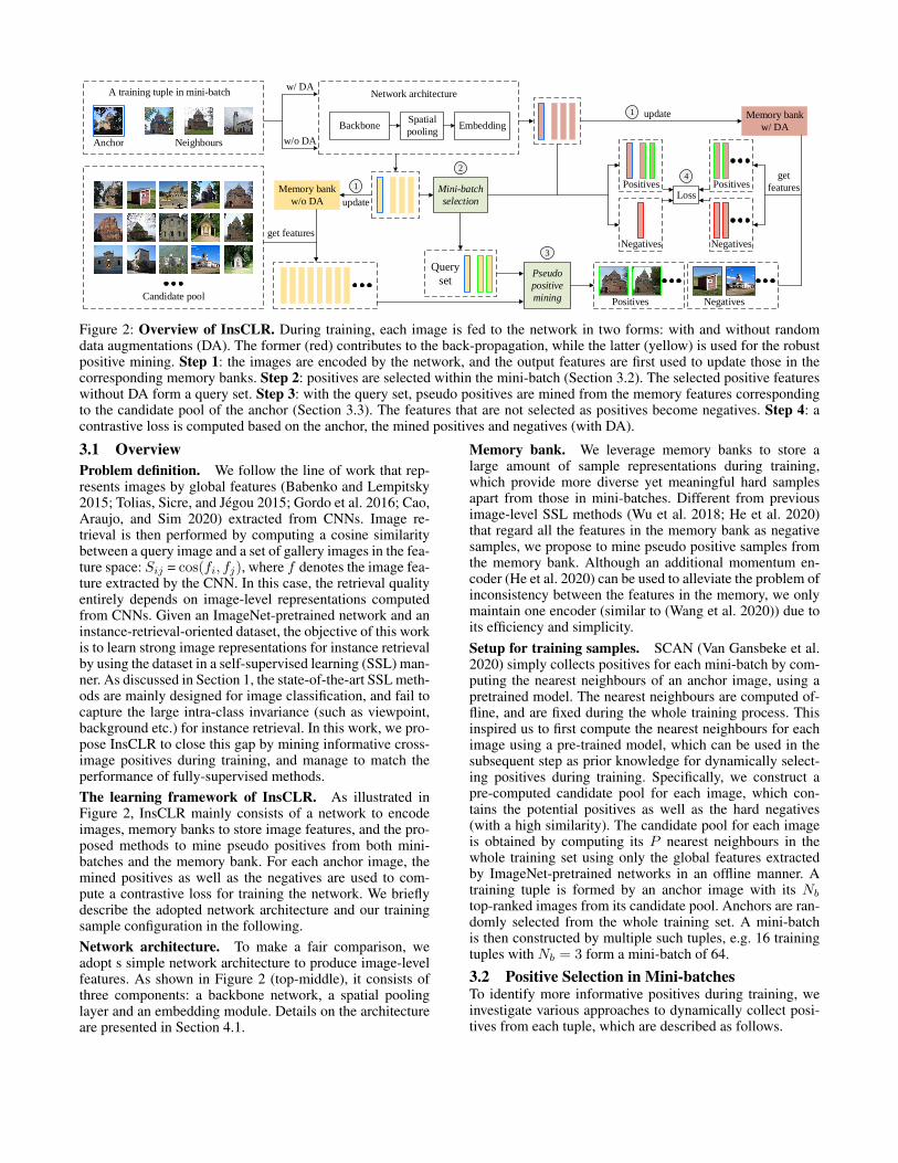
Figure 2: Overview of InsCLR. During training, each image is fed to the network in two forms: with and without randomdata augmentations (DA). The former (red) contributes to the back-propagation, while the latter (yellow) is used for the robustpositive mining. Step 1: the images are encoded by the network, and the output features are first used to update those in thecorresponding memory banks. Step 2: positives are selected within the mini-batch (Section 3.2). The selected positive featureswithout DA form a query set. Step 3: with the query set, pseudo positives are mined from the memory features correspondingto the candidate pool of the anchor (Section 3.3). The features that are not selected as positives become negatives. Step 4: acontrastive loss is computed based on the anchor, the mined positives and negatives (with DA).
3.1 OverviewProblem definition. We follow the line of work that rep-resents images by global features (Babenko and Lempitsky2015; Tolias, Sicre, and Jegou 2015; Gordo et al. 2016; Cao,Araujo, and Sim 2020) extracted from CNNs. Image re-trieval is then performed by computing a cosine similaritybetween a query image and a set of gallery images in the fea-ture space: Sij = cos(fi, fj), where f denotes the image fea-ture extracted by the CNN. In this case, the retrieval qualityentirely depends on image-level representations computedfrom CNNs. Given an ImageNet-pretrained network and aninstance-retrieval-oriented dataset, the objective of this workis to learn strong image representations for instance retrievalby using the dataset in a self-supervised learning (SSL) man-ner. As discussed in Section 1, the state-of-the-art SSL meth-ods are mainly designed for image classification, and fail tocapture the large intra-class invariance (such as viewpoint,background etc.) for instance retrieval. In this work, we pro-pose InsCLR to close this gap by mining informative cross-image positives during training, and manage to match theperformance of fully-supervised methods.The learning framework of InsCLR. As illustrated inFigure 2, InsCLR mainly consists of a network to encodeimages, memory banks to store image features, and the pro-posed methods to mine pseudo positives from both mini-batches and the memory bank. For each anchor image, themined positives as well as the negatives are used to com-pute a contrastive loss for training the network. We brieflydescribe the adopted network architecture and our trainingsample configuration in the following.Network architecture. To make a fair comparison, weadopt s simple network architecture to produce image-levelfeatures. As shown in Figure 2 (top-middle), it consists ofthree components: a backbone network, a spatial poolinglayer and an embedding module. Details on the architectureare presented in Section 4.1.
Memory bank. We leverage memory banks to store alarge amount of sample representations during training,which provide more diverse yet meaningful hard samplesapart from those in mini-batches. Different from previousimage-level SSL methods (Wu et al. 2018; He et al. 2020)that regard all the features in the memory bank as negativesamples, we propose to mine pseudo positive samples fromthe memory bank. Although an additional momentum en-coder (He et al. 2020) can be used to alleviate the problem ofinconsistency between the features in the memory, we onlymaintain one encoder (similar to (Wang et al. 2020)) due toits efficiency and simplicity.Setup for training samples. SCAN (Van Gansbeke et al.2020) simply collects positives for each mini-batch by com-puting the nearest neighbours of an anchor image, using apretrained model. The nearest neighbours are computed of-fline, and are fixed during the whole training process. Thisinspired us to first compute the nearest neighbours for eachimage using a pre-trained model, which can be used in thesubsequent step as prior knowledge for dynamically select-ing positives during training. Specifically, we construct apre-computed candidate pool for each image, which con-tains the potential positives as well as the hard negatives(with a high similarity). The candidate pool for each imageis obtained by computing its P nearest neighbours in thewhole training set using only the global features extractedby ImageNet-pretrained networks in an offline manner. Atraining tuple is formed by an anchor image with its Nb
top-ranked images from its candidate pool. Anchors are ran-domly selected from the whole training set. A mini-batchis then constructed by multiple such tuples, e.g. 16 trainingtuples with Nb = 3 form a mini-batch of 64.
3.2 Positive Selection in Mini-batchesTo identify more informative positives during training, weinvestigate various approaches to dynamically collect posi-tives from each tuple, which are described as follows.

We consider taking all the Nb images in the tuple aspositives, referred as nn (similar to (Van Gansbeke et al.2020)), as a baseline. We then investigate four threshold-based strategies to select the positives from the Nb images.Given a threshold Tb, the four methods are defined as fol-lows.
(1) Augmented similarity. We adopt a threshold to se-lect the positives, i.e. computing feature similarities betweenthe anchor and Nb neighboring images in the training tuple,and only considering the images with a similarity over thepredefined threshold as pseudo positives: SDA
ij > Tb. How-ever, this similarity is highly unreliable since it is computedusing the images after random augmentations. (2) Unaug-mented similarity. To overcome this limitation, the secondstrategy is to feed the original images without any augmen-tation to the networks, and apply the threshold on their sim-ilarities: Sw/oDA
ij > Tb. Note that the unaugmented versionis only used for similarity computation, and does not con-tribute to training loss. (3) Sample-relative similarity. Auniversal threshold may not work reliably to all anchor im-ages. Some classes may have smaller intra-class variance,and thus require larger thresholds. We further develop thethird strategy that selects the positives by using sample-relative similarities. Namely, the similarities are scaled bydividing by the largest similarity in each training tuple: Srel
ij> Tb. (4) Multi-scale similarity. Lastly, based on the sec-ond strategy, we intend to improve the similarity by feedingthe unaugmented images with multiple scales, which is thefourth strategy: Sms
ij > Tb.With these mining approaches, we can select pseudo pos-
itives dynamically within each mini-batch. For example, atraining tuple with Nb = 7 may have 3 images selected aspositives, based on one of the proposed methods, and theother 4 are then regarded as negatives. We empirically com-pare the four strategies in Section 4.2.
3.3 Mining Positives from Memory BankBenefits. Apart from learning the discrimination betweenpositives and negatives in mini-batches, we also wish tocollect more positives from the memory bank. The bene-fit of finding positives from the memory bank is two-fold.First, mining more positives from the memory bank willencourage the model to pull potential positives closer, in-stead of pushing them away by default (i.e. considering themas negatives in the memory). This sets our method apartfrom image-level SSL like MoCo (He et al. 2020) or Sim-CLR (Chen et al. 2020a). Second, by excluding the selectedpositives, the rest of the images in the candidate pool areconsidered as hard negatives, since they often have high of-fline similarities with the anchor image (comparing to otherimages in the dataset).Mining with query sets. The selected positives within themini-batch are assumed to be of the same class as the anchor,with a high confidence. Therefore, we can consider the an-chor image and its selected positives from the mini-batch asa query set, and then cast the task of mining positives fromthe memory bank into a retrieval problem with a set of queryimages, instead of a single query image. To this end, we pro-pose a new algorithm that can effectively explore the under-
Selected pesudo positive from mini-batch
Candidate
0.8
Similarity aggregationSimilarity computation
Query
set
0.75
Query
set
Query set
for iter k+1
Anchor
Mined pesudo positive from candidate pool
Determine pseudo positives
Iter k
Sset
Image manifold
Figure 3: Mining positives in the memory bank. The sim-ilarities Sset between each image in the candidate pool andthe whole query set are computed by pairwise similaritycomputation followed by aggregation. The positive selectionis based on Sset and the mined images become part of thenew query set.
lying image relation on-the-fly during training. This proce-dure is presented in the bottom part of Figure 2. Crucially,the whole mining process should be performed on the imagefeatures extracted without any random augmentation. Other-wise, we found the training can degrade significantly. Hence,two memory banks are used. The one without augmentationsis for mining, while the other one is for representation learn-ing. To be specific, our method consists of two steps: simi-larity computation and aggregation, which are performed onevery training tuple in a mini-batch. The method is shown inFigure 3.Step 1: similarity computation. To make use of everyquery at hand, we first compute the similarity between thefeatures of each query image and that of memory images.Each image in the pool now has Np similarity scores, whereNp denotes the size of the query set Q. As an optional step,we can disregard the similarity scores below a threshold. In-tuitively, it is possible to have an image which may not looksimilar to all the images of the same class, e.g. even thoughimages contain the same object, they may not have a lowglobal similarity due to different viewpoint and backgroundclutter etc. Mathematically, we have:
S(i, Q) = φ(S(i, q1), S(i, q2), . . . , S(i, qNp)), (1)
where φ is the optional discarding step and q ∈ Q.Step 2: similarity aggregation. For each image in thecandidate pool, we measure its similarity to the whole queryset by Sset. Sset is obtained by aggregating its similaritiesto each image in the query set. In this work, two aggregationfunctions are considered: average and maximum:
Sset = ψ(S(i, Q)), (2)
where ψ is the aggregation function. We then re-rank theimages in the candidate pool based on Sset. Given the re-ranked of candidate images, we can determine the pseudo

positives either using a threshold Tm or the top-k rule. Themined positives can be added to the query set Q and we canrepeat the above two steps for several times to gather morepositives if desired. Apart from the mined positives, the restof the candidate pool is then used as negatives.
Efficient online graph traversal. The proposed methodcan be considered as an online graph traversal in the imagemanifold of the query set and the candidate pool. It has twoadvantages comparing to the standard offline graph traversalmethods like (Iscen et al. 2017, 2018; Chang et al. 2019).First, it can be applied during training without introducingmuch computational overhead. It avoids computing the sim-ilarities among images in the candidate pool. Instead, sim-ilarities are only measured between the candidate pool andthe query set. Second, it is an online approach and the im-age manifolds can become more reliable along the training,in contrast to (Iscen et al. 2018) in which the image labelsare generated in the fixed image manifolds before training.
3.4 LossWe adopt a simple contrastive loss (Hadsell, Chopra, andLeCun 2006). Concretely, the loss function L for a trainingtuple is:
L =1
Np
Np∑i=1
Niter∑yi 6=yj
Sij −Niter∑yi=yj
Sij
, (3)
where Np is the size of query set after memory mining. Fora training iteration, Niter is a collection of all images inthe mini-batch and the candidate pool for the anchor image.yi 6= yj indicates a negative pair while yi = yj denotes apositive pair. Sij is the cosine similarity between features.
4 Experiments and Results4.1 Implementation DetailsNetwork architecture. Following (Weyand et al. 2020),ResNet-101 (He et al. 2016) is used as the backbone net-work, and only the first four convolutional blocks are kept.The channel size of the backbone output feature map is2048. For the spatial pooling layer, we adopt the GeneralizedMean pooling (Radenovic, Tolias, and Chum 2018) (GeM)with the parameter p fixed to be 3. Similar to (Gordo et al.2017; Cao, Araujo, and Sim 2020), we use a fully-connectedlayer as the embedding module with an output dimension of2048, without a careful tuning.
Training details. The training data is a subset ofGLDv2 (Ozaki and Yokoo 2019). The dataset contains 1.2Mimages from 27k landmarks. Unless specified, the size of theoffline-computed candidate pool P is set to be 500 for everyimage, and Nb is set to be 3 for all networks. More detailsregarding the training and the evaluation protocol (includingfeature extraction) refer to the supplementary material.
4.2 Ablation studyWe conduct ablation study on two public benchmarks: Ox-ford and Paris with revisited annotations (Radenovic et al.2018), denoted byROxf andRPar, respectively.
Method Batch Memory Medium Hard
ROxf RPar ROxf RParImageNet 23.0 52.0 6.5 25.9ImageNet + PCA 40.9 65.6 30.5 41.7ImageNet + PCA∗ 45.0 70.7 17.7 48.7Supervised-Arc† 76.2 86.8 55.1 72.5
A nn - 57.6 68.1 30.3 43.7B nn neg. 61.0 73.4 35.4 52.6C ours neg. 65.2 75.1 39.9 55.7D-anchor ours anc. 67.4 75.6 42.2 56.5D ours ours 73.1 77.6 48.3 59.5
Table 1: Ablation on pseudo positive mining. All meth-ods use ResNet-101 with GeM pooling. nn denotes that tak-ing all the images in the training tuple as positives withoutselection. neg. means that all of the 105 features randomlysampled from the memory bank are considered as negatives.* is from (Radenovic et al. 2018), and † is from (Weyandet al. 2020) trained with ArcFace loss (Deng et al. 2019).
Candidate pool size. We empirically find that the perfor-mance increases along with P until around 250, after whichthe performance improves marginally. This is probably be-cause only the hard negatives with similarity higher than 0.4contribute to the loss, and increasing the size of the pool over200 brings minimal hard negatives.Positive selection in mini-batches. As Figure 4 shows,the proposed pseudo positive selection strategies improvethe performance over the nearest-neighbour baseline nn ingeneral. In particular, applying an absolute threshold on theunaugmented similarity performs better than others, onlybeaten by its multi-scale variant on RPar. Furthermore, thesimilarity based on the augmented images is highly unre-liable and harms the retrieval performance severely. Thisproves the importance of feeding a version without dataaugmentation for each image during training. Based on theunaugmented similarity, we experiment on several values ofNb (i.e. 1, 3, 5, 7), and find thatNb = 3 is the optimal choice.In the rest of the experiments, a threshold of Tb = 0.65 withthe unaugmented similarity is adopted, with Nb = 3.Performance gain of each component. We compare ourmethod with several baselines and show the performancegain brought by each proposed component in Table 1.Firstly, the ImageNet-pretrained network can be seen as alower bound. As reported in (Radenovic et al. 2018), apply-ing a PCA/whitening on the features can significantly in-crease the performance. Notably, the rest of the results inTable 1 do not involve PCA post-processing. Training withoffline-computed nn positives in the mini-batch (denoted bymethod A) raises the performance to a relatively high level,i.e. above 60 with medium setup. Method B is method Awith a memory bank in which features are only regarded asnegatives. This gives notable gains in bothROxf andRPar.Method C replaces the nnwith the proposed pseudo positiveselection, which improves the mAP by around 4 and 3 pointsin ROxf and RPar, respectively. If the proposed memorymining is adopted (denoted by method D), the performanceis further boosted prominently. However, if we perform themining in the memory only using the anchor image itself(i.e. without the selected positives in the training tuple), the

Figure 4: Ablation on the positive selection in mini-batches. The results are obtained on ROxf (left) and RPar (right) withmedium protocol. nn considers all the Nb images in each training tuple to be positives, without selection. Notably, the resultsof augmented-image-based similarity are not shown in the plots: 35.7 mAP and 39.5 mAP forROxf andRPar, respectively.
Aggre. SelectionMedium Hard
ROxf RPar ROxf RParavg topk 71.3 77.0 45.5 58.3avg topk w/ spa. 70.4 77.1 44.8 58.8avg threshold 68.4 76.3 42.0 57.4max topk 70.6 77.2 44.5 58.7max topk w/ spa. 70.4 77.2 44.0 58.5max threshold 61.1 71.5 34.9 47.6avg topk 1× 69.5 76.2 42.8 57.2avg topk 4× 73.1 77.6 48.3 59.5
Table 2: Ablation on mining positives in the memorybank. topk denotes taking the top k = 5 images in theranked candidate pool. Tm = 0.6 for threshold. spa. refersto retaining only the similarity scores above 0.6 to enforcethe sparsity. 1× or 4× means that the mining is performedfor one or four iterations (otherwise two iterations).
performance drops significantly. This validates the impor-tance of mining with a query set.Details in memory mining. In Table 2, we compare thedifferent options in the design of memory mining describedin Section 3.3. For the similarity aggregation methods, meanand max perform better inROxf andRPar, respectively. Asthe selection strategy, topk performs better than threshold.This is in contrast to the case in mini-batches, where thresh-old is better. It is because the potential positives from mini-batches are the top-ranked images from the candidate pool,which are very likely to be easy positives. Hence, the takingthresholds on the similarity is relatively reliable. Whereas inthe memory bank, mining is more difficult and similaritiesbecome less reliable. In terms of sparsity, the performanceseems not sensitive. This is probably because the size ofthe query set is relatively small. The last conclusion to drawfrom Table 2 is that the mAP increases with the mining it-erations, while bringing negligible computational overhead.In the rest of the experiments, avg and topk are adopted with4 iterations in the mining.Mining accuracy at training. We analyze the precisionof positive mining along the training, which is defined as theratio between the true positives mined and the total num-ber of mined pseudo positives. We find that the precision ofmining in both mini-batches and the memory bank increases
gradually along the training. The plots of the precision aredisplayed in the supplementary material.4.3 Comparison with other methodsWe compare InsCLR with the state-of-the-art methods in Ta-ble 3, including the large-scale retrieval results by addingR1M. Following the convention in image retrieval and fora fair comparison, all the self-supervised methods (includ-ing SimCLR, MoCov2, SwAV etc.) start with ImageNet-pretrained networks and are used to fine-tune on GLDv2.Supervised methods. Table 3 shows that InsCLRachieves outstanding mAP on ROxf and RPar for bothmedium and hard setup. In particular, the mAP of InsCLRon ROxf medium is on par with the state-of-the-art super-vised methods. Namely, only R101-GeM (GLDv2-clean)performs better than InsCLR on bothROxf andRPar, whenspatial verification (SP) is not considered. In particular,with the same architecture, InsCLR enhances the mAP onROxf medium/hard from 45.0/17.7 (ImageNet pretrained)to 73.1/48.3, comparing to 76.2/55.1 attained with fullsupervision. Even with SP, DELF-R-ASMK+SP (GLD) onlyperforms better than InsCLR whenR1M is added. However,SP is much slower at run-time and memory-consuming.
Self-supervised methods. In the self-supervised regime,InsCLR surpasses all the self-supervised methods. We at-tempted to train SCAN on our task but it failed to convergein the clustering step (probably due to the large number ofclasses and significant intra-class variance). Lastly, althoughclustering-based methods like DeepCluster, PCL and SwAVimplicitly take into account the intra-class variation into therepresentation learning, they hardly bring improvements. Itshows that learning intra-class invariance explicitly frompositive and negative pairs is superior for the task at hand.Moreover, as Table 4 shows, InsCLR achieves significantlyhigher mAP than (Iscen et al. 2018) on the original Oxfordand Paris dataset.
4.4 Evaluation on More BenchmarksGLDv2 retrieval task. We directly evaluate the trainedInsCLR model on a recently released large-scale bench-mark, namely, the GLDv2 retrieval task. As shown in Ta-ble 5, InsCLR can achieve performance 13.39% and 13.71%

MethodMedium Hard
ROxf +R1M RPar +R1M ROxf +R1M RPar +R1MSupervised training
R101 - GeM (ImageNet) (Radenovic et al. 2018) 45.0 25.6 70.7 46.2 17.7 4.7 48.7 20.3R101 - R-MAC (Gordo et al. 2017) 60.9 39.3 78.9 54.8 32.4 12.5 59.4 28.0R101 - GeM - AP (Revaud et al. 2019) 67.5 47.5 80.1 52.5 42.8 23.2 60.5 25.1R101 - GeM - AP (GLD) (Revaud et al. 2019) 66.3 – 80.2 – 42.5 – 60.8 –R101 - DELG (Cao, Araujo, and Sim 2020) 73.2 54.8 82.4 61.8 51.2 30.3 64.7 35.5R101 - GeM (GLDv2-clean) (Weyand et al. 2020) 76.2 - 86.8 - 55.1 - 72.5 -DELF - ASMK + SP (Radenovic et al. 2018) 67.8 53.8 76.9 57.3 43.1 31.2 55.4 26.4DELF - R-ASMK + SP (GLD) (Teichmann et al. 2019) 76.0 64.0 80.2 59.7 52.4 38.1 58.6 29.4
Self-supervised training based on automatic annotationVGG16 - MAC (Radenovic, Tolias, and Chum 2016) 58.4 39.1 66.8 42.4 30.5 17.9 42.0 17.7R101 - GeM (GLD) (Radenovic, Tolias, and Chum 2018) 64.7 45.2 77.2 52.3 38.5 19.9 56.3 24.7R152 - GeM (GLD) (Radenovic, Tolias, and Chum 2018) 68.7 – 79.7 – 44.2 – 60.3 –R101 - GeM (Simeoni, Avrithis, and Chum 2019) 65.3 46.1 77.3 52.6 39.6 22.2 56.6 24.8R101 - GeM + DSM (Simeoni, Avrithis, and Chum 2019) 65.3 47.6 77.4 52.8 39.2 23.2 56.2 25.0
Self-supervised trainingDeepCluster (Caron et al. 2018) 29.8 9.8 49.1 13.3 9.0 0.9 26.0 3.2SimCLR (Chen et al. 2020a) 22.2 9.4 50.5 14.4 6.3 2.2 19.6 1.1MoCov2 (Chen et al. 2020b) 27.3 11.0 65.1 17.4 6.1 0.8 38.4 3.2BYOL (Grill et al. 2020) 11.0 1.9 28.4 3.7 2.3 0.1 8.8 0.2PCL (Li et al. 2020) 29.2 10.3 59.3 17.6 7.9 0.5 28.9 2.6SwAV (Caron et al. 2020) 19.9 7.1 38.5 10.4 3.7 0.1 10.5 0.4InsCLR (ours) 73.1 56.2 77.6 56.7 48.3 29.6 59.5 29.2
Table 3: Comparison to state-of-the-art methods on large-scale retrieval. Automatic annotation means additional computervision systems are used to annotate the images before training. SP refers to the spatial verification using local features. Results ofall the unsupervised methods are obtained using their official code with careful hyper-parameter tuning, with the same networkarchitecture as InsCLR. Note that all the methods in this table are built on ImageNet-pretrained networks.
Method Oxf5k Oxf105k Paris6k Paris106k(Iscen et al. 2018) 78.2 72.6 85.1 78.0InsCLR 92.0 91.4 94.2 90.5Table 4: Evaluation on original Oxford5k and Paris6k.
Method Labels Validation set Test set(Weyand et al. 2020) Yes 23.30 25.57ImageNet pretrained No 0.89 0.52InsCLR No 13.39 13.71
Table 5: Retrieval task on GLDv2 (% mAP@100).
on validation and test set, respectively. This is a surprisinglylarge improvement comparing to the ImageNet-pretrainedbaseline, given that no labels are used.
INSTRE benchmark. To showcase the generalization ofInsCLR, we fine-tune an ImageNet-pretrained ResNet-50with GeM (p = 3) on another instance retrieval benchmark:INSTRE (Wang and Jiang 2015). We adopt the same train-test splitting as (Iscen et al. 2017, 2018) for a fair compari-son. As shown by Table 6, InsCLR significantly outperforms(Iscen et al. 2018) and even (Iscen et al. 2017) which uses la-bels and ResNet-101. Moreover, the proposed positive min-ing within mini-batches and the memory again boosts theperformance by a large margin (i.e. 55.6 to 76.2).
4.5 Qualitative AnalysisWe further conduct qualitative analysis to demonstrate thatInsCLR can learn better representations for instance re-trieval in terms of viewpoint-invariance than previous SSLmethods. As we can see from Figure 5, InsCLR can retrievemore correct images, and some of them have significantly
Method Fine-tuning Labels INSTREImageNet (w/o PCA) - - 32.7(Iscen et al. 2017)† Landmarks Yes 62.6(Iscen et al. 2018) INSTRE No 57.7InsCLR w/o P.M. (nn=1) INSTRE No 55.6InsCLR INSTRE No 76.2
Table 6: Evaluation on INSTRE. † denotes the result ofmethod (Gordo et al. 2017) implemented by (Iscen et al.2017). P.M. denotes the positive mining in InsCLR.
Query
Query
Figure 5: InsCLR (top) vs. MoCov2 (bottom). The top 5retrieved images by InsCLR are all correct (green). Some ofthem have very different viewpoint to the query image.
different viewpoints with the query image.
5 ConclustionWe present a new SSL method built on the instance-levelconstrastive learning for instance retrieval. This sets it apartfrom existing SSL methods that commonly learn fromimage-level contrast. InsCLR can learn intra-class invari-ance by dynamically mining informative positives from bothmini-batches and memory bank during training. Extensiveexperiments demonstrate that InsCLR can achieve compara-ble performance to supervised methods on instance retrieval.

ReferencesArandjelovic, R.; Gronat, P.; Torii, A.; Pajdla, T.; and Sivic,J. 2016. NetVLAD: CNN architecture for weakly supervisedplace recognition. In Proceedings of the IEEE conference oncomputer vision and pattern recognition, 5297–5307.
Babenko, A.; and Lempitsky, V. 2015. Aggregating deepconvolutional features for image retrieval. arXiv preprintarXiv:1510.07493.
Cao, B.; Araujo, A.; and Sim, J. 2020. Unifying Deep Localand Global Features for Image Search. arXiv, arXiv–2001.
Caron, M.; Bojanowski, P.; Joulin, A.; and Douze, M. 2018.Deep clustering for unsupervised learning of visual features.In Proceedings of the European Conference on ComputerVision (ECCV), 132–149.
Caron, M.; Misra, I.; Mairal, J.; Goyal, P.; Bojanowski, P.;and Joulin, A. 2020. Unsupervised learning of visual fea-tures by contrasting cluster assignments. arXiv preprintarXiv:2006.09882.
Chang, C.; Yu, G.; Liu, C.; and Volkovs, M. 2019. Explore-exploit graph traversal for image retrieval. In Proceedingsof the IEEE Conference on Computer Vision and PatternRecognition, 9423–9431.
Chen, T.; Kornblith, S.; Norouzi, M.; and Hinton, G. 2020a.A simple framework for contrastive learning of visual repre-sentations. arXiv preprint arXiv:2002.05709.
Chen, X.; Fan, H.; Girshick, R.; and He, K. 2020b. Improvedbaselines with momentum contrastive learning. arXivpreprint arXiv:2003.04297.
Chum, O.; Philbin, J.; Sivic, J.; Isard, M.; and Zisserman, A.2007. Total recall: Automatic query expansion with a gener-ative feature model for object retrieval. In 2007 IEEE 11thInternational Conference on Computer Vision, 1–8. IEEE.
Deng, J.; Guo, J.; Xue, N.; and Zafeiriou, S. 2019. Arcface:Additive angular margin loss for deep face recognition. InProceedings of the IEEE Conference on Computer Visionand Pattern Recognition, 4690–4699.
Gordo, A.; Almazan, J.; Revaud, J.; and Larlus, D. 2016.Deep image retrieval: Learning global representations forimage search. In European conference on computer vision,241–257. Springer.
Gordo, A.; Almazan, J.; Revaud, J.; and Larlus, D. 2017.End-to-end learning of deep visual representations for imageretrieval. International Journal of Computer Vision, 124(2):237–254.
Grill, J.-B.; Strub, F.; Altche, F.; Tallec, C.; Richemond,P.; Buchatskaya, E.; Doersch, C.; Avila Pires, B.; Guo, Z.;Gheshlaghi Azar, M.; et al. 2020. Bootstrap Your OwnLatent-A New Approach to Self-Supervised Learning. Ad-vances in Neural Information Processing Systems, 33.
Hadsell, R.; Chopra, S.; and LeCun, Y. 2006. Dimension-ality reduction by learning an invariant mapping. In 2006IEEE Computer Society Conference on Computer Visionand Pattern Recognition (CVPR’06), volume 2, 1735–1742.IEEE.
He, K.; Fan, H.; Wu, Y.; Xie, S.; and Girshick, R. 2020.Momentum contrast for unsupervised visual representationlearning. In Proceedings of the IEEE/CVF Conference onComputer Vision and Pattern Recognition, 9729–9738.He, K.; Zhang, X.; Ren, S.; and Sun, J. 2016. Deep resid-ual learning for image recognition. In Proceedings of theIEEE conference on computer vision and pattern recogni-tion, 770–778.Iscen, A.; Tolias, G.; Avrithis, Y.; and Chum, O. 2018. Min-ing on manifolds: Metric learning without labels. In Pro-ceedings of the IEEE Conference on Computer Vision andPattern Recognition, 7642–7651.Iscen, A.; Tolias, G.; Avrithis, Y.; Furon, T.; and Chum, O.2017. Efficient diffusion on region manifolds: Recoveringsmall objects with compact cnn representations. In Pro-ceedings of the IEEE Conference on Computer Vision andPattern Recognition, 2077–2086.Kingma, D. P.; and Ba, J. 2014. Adam: A method forstochastic optimization. arXiv preprint arXiv:1412.6980.Li, J.; Zhou, P.; Xiong, C.; Socher, R.; and Hoi, S. C. 2020.Prototypical contrastive learning of unsupervised represen-tations. arXiv preprint arXiv:2005.04966.Li, S.; Chen, D.; Liu, B.; Yu, N.; and Zhao, R. 2019.Memory-based neighbourhood embedding for visual recog-nition. In Proceedings of the IEEE International Conferenceon Computer Vision, 6102–6111.Noh, H.; Araujo, A.; Sim, J.; Weyand, T.; and Han, B. 2017.Large-scale image retrieval with attentive deep local fea-tures. In Proceedings of the IEEE international conferenceon computer vision, 3456–3465.Oord, A. v. d.; Li, Y.; and Vinyals, O. 2018. Representationlearning with contrastive predictive coding. arXiv preprintarXiv:1807.03748.Ozaki, K.; and Yokoo, S. 2019. Large-scale landmark re-trieval/recognition under a noisy and diverse dataset. arXivpreprint arXiv:1906.04087.Philbin, J.; Chum, O.; Isard, M.; Sivic, J.; and Zisserman,A. 2007. Object retrieval with large vocabularies and fastspatial matching. In Proceedings of the IEEE Conferenceon Computer Vision and Pattern Recognition, 1–8. IEEE.Radenovic, F.; Iscen, A.; Tolias, G.; Avrithis, Y.; and Chum,O. 2018. Revisiting oxford and paris: Large-scale imageretrieval benchmarking. In Proceedings of the IEEE Con-ference on Computer Vision and Pattern Recognition, 5706–5715.Radenovic, F.; Tolias, G.; and Chum, O. 2016. CNN imageretrieval learns from BoW: Unsupervised fine-tuning withhard examples. In European conference on computer vision,3–20. Springer.Radenovic, F.; Tolias, G.; and Chum, O. 2018. Fine-tuningCNN image retrieval with no human annotation. IEEE trans-actions on pattern analysis and machine intelligence, 41(7):1655–1668.Revaud, J.; Almazan, J.; Rezende, R. S.; and Souza, C. R. d.2019. Learning with average precision: Training image re-trieval with a listwise loss. In Proceedings of the IEEE In-ternational Conference on Computer Vision, 5107–5116.
Schonberger, J. L.; and Frahm, J.-M. 2016. Structure-from-motion revisited. In Proceedings of the IEEE Conference onComputer Vision and Pattern Recognition, 4104–4113.Simeoni, O.; Avrithis, Y.; and Chum, O. 2019. Local fea-tures and visual words emerge in activations. In Proceed-ings of the IEEE Conference on Computer Vision and Pat-tern Recognition, 11651–11660.Teichmann, M.; Araujo, A.; Zhu, M.; and Sim, J. 2019.Detect-to-retrieve: Efficient regional aggregation for imagesearch. In Proceedings of the IEEE Conference on ComputerVision and Pattern Recognition, 5109–5118.Tolias, G.; Avrithis, Y.; and Jegou, H. 2016. Image searchwith selective match kernels: aggregation across single andmultiple images. International Journal of Computer Vision,116(3): 247–261.Tolias, G.; Sicre, R.; and Jegou, H. 2015. Particular ob-ject retrieval with integral max-pooling of CNN activations.arXiv preprint arXiv:1511.05879.Van Gansbeke, W.; Vandenhende, S.; Georgoulis, S.; Proes-mans, M.; and Van Gool, L. 2020. Scan: Learning to classifyimages without labels. In European Conference on Com-puter Vision, 268–285. Springer.Wang, S.; and Jiang, S. 2015. INSTRE: a new benchmarkfor instance-level object retrieval and recognition. ACMTransactions on Multimedia Computing, Communications,and Applications (TOMM), 11(3): 1–21.Wang, X.; Zhang, H.; Huang, W.; and Scott, M. R. 2020.Cross-Batch Memory for Embedding Learning. In Proceed-ings of the IEEE/CVF Conference on Computer Vision andPattern Recognition, 6388–6397.Weyand, T.; Araujo, A.; Cao, B.; and Sim, J. 2020.Google Landmarks Dataset v2-A Large-Scale Benchmarkfor Instance-Level Recognition and Retrieval. In Proceed-ings of the IEEE/CVF Conference on Computer Vision andPattern Recognition, 2575–2584.Wu, Z.; Xiong, Y.; Yu, S. X.; and Lin, D. 2018. Unsuper-vised feature learning via non-parametric instance discrimi-nation. In Proceedings of the IEEE Conference on ComputerVision and Pattern Recognition, 3733–3742.Xie, J.; Zhan, X.; Liu, Z.; Ong, Y. S.; and Loy, C. C. 2020.Delving into Inter-Image Invariance for Unsupervised Vi-sual Representations. arXiv preprint arXiv:2008.11702.

6 Supplementary Material6.1 Relation to Set-based Retrieval MethodsOther solution to tackle query-set-based image retrieval in-cludes using the query expansion (Chum et al. 2007). How-ever, only global features (i.e. no local features) are consid-ered in our case, and thus the query expansion boils downto ranking the candidate pool using the averaged image fea-tures of the whole query set. Another line of work that canimprove a retrieval recall is to construct a similarity graph,and then explore the underlying image relation on man-ifolds using diffusion (Iscen et al. 2017, 2018) or graphtraversal (Chang et al. 2019). Unfortunately, this line of ap-proaches are usually computationally expensive in both of-fline (e.g. the similarity graph construction) and online situ-ations (e.g. the graph traversal).
6.2 Details of the LossAs mentioned in the main paper, we adopt a simple con-trastive loss (Hadsell, Chopra, and LeCun 2006). Con-cretely, the loss function L for a training tuple can be com-puted as:
L =1
Np
Np∑i=1
Niter∑yi 6=yj
Sij −Niter∑yi=yj
Sij
, (4)
where Np is the number of selected pseudo positives plus ananchor image in a training tuple, defined as a ‘query set’ formemory mining. Notice that a training mini-batch includesmultiple training tuples, e.g., a mini-batch of 64 images con-tains 8 training tuples of size 8. For a training iteration,Niter
is a collection of all images in the mini-batch and the candi-date pool for the anchor image. For the loss computation,the negatives include (1) all the remained images not se-lected as pseudo positives in the training tuple, (2) all theimages in other training tuples in the same mini-batch, and(3) all the images in the candidate pool (excluding the minedpositives). yi 6= yj indicates a negative pair while yi = yjdenotes a positive pair. Sij is the cosine similarity betweenthe features of an image pair. As described in the main paper,only negatives with a similarity higher than 0.4 (between itspaired image) can contribute to the loss.
6.3 Network Architecture in DetailHere we explain the network architecture adopted in thiswork in detail. The network architecture consists of threecomponents: a backbone network, a spatial pooling layerand an embedding module. Given an input image, the back-bone network is used to encode it to a feature map of sizeCb×H×W , where Cb is the number of channels andH,Ware the height and width of the feature map, respectively. Thefeature map is then fed into a spatial pooling layer to givea Cb × 1 dimensional feature vector. This feature vector isL2-normalized and passed to the embedding module whichoutputs a Ce × 1 dimensional feature. The embedding mod-ule acts as a similar role to PCA or whitening, but can betrained with the network in an end-to-end fashion. Finally,
the image representation is obtained by L2-normalizing theembedded feature.
Following (Weyand et al. 2020), ResNet-101 (He et al.2016) is used as the backbone network, and only the firstfour convolutional blocks are kept. In this case, Cb = 2048.The backbone is initialized with pretrained weights on Im-ageNet. For the spatial pooling layer, we adopt the Gener-alized Mean pooling (Radenovic, Tolias, and Chum 2018)(GeM) with the parameter p fixed to be 3. Similar to (Gordoet al. 2017; Cao, Araujo, and Sim 2020), we use a fully-connected layer as the embedding module with Ce being2048, without a careful tuning.
6.4 Training DetailsTraining InsCLR. Data augmentations for training im-ages include random cropping with a range of scale be-ing 0.4 to 1.0 and aspect ratio being 0.75 to 1.33, fol-lowed by a resizing. The horizontal flipping with a chanceof 50% is also applied. The network is optimized usingAdam (Kingma and Ba 2014). The training of InsCLR con-sists of two rounds of training, between which the candi-date pool is updated. Namely, the candidate pool for the firstround is obtained using the ImageNet-pretrained network,and that of the second round is obtained using the networkat the end of the first round training. For the first round, theaugmented input images are resized to 224 × 224 with abatch size of 200. For the second round, the augmented in-put images are resized to 448× 448 with a batch size of 64.In this case, each mini-batch contains 16 training tuples withNb = 3. The size of the unaugmented images during train-ing is fixed to be 512 × 512. The training iteration of thefirst round is 60k with an initial learning rate of 10−4 anddivided by 10 after 30k and 45k iterations. The training iter-ation of the second round is 40k, with an initial learning rateof 3 × 10⁻⁵ and divided by 10 at 20k. The weight decay is10−4.
Implementation details for other methods. All the ex-isting methods are implemented using the official code orwidely-used PyTorch implementations with careful hyper-parameter tuning. Namely, MoCov2 is implemented usingthe official codebase *. PCL is implemented using the of-ficial codebase †. SwAV is implemented using the officialcodebase ‡. DeepCluster, SimCLR and BYOL are imple-mented using the well-maintained repository §. For Sim-CLR, MoCov2, BYOL, PCL and SwAV, we follow the offi-cial training scheme, including the learning rate scheme anddata augmentations etc., and the network is trained for 20epochs. We also try to train with these methods using dif-ferent learning rates, and report with the best model. Theoptimal initial learning rate of these five methods are 0.3,0.03, 0.2, 0.03, 0.03, respectively. For DeepClusters, we setthe number of classes to be 30k, and train the network for 20epochs with a learning of 0.15. The image pseudo labels andclassifier are updated after each epoch. All the methods are
*https://github.com/facebookresearch/moco†https://github.com/salesforce/PCL‡https://github.com/facebookresearch/swav§https://github.com/open-mmlab/OpenSelfSup

Figure 6: Analysis of pseudo positives mined from the mini-batch (left) or memory bank (right) during training (of the secondround). Top: the number of pseudo positives (for each anchor image) collected from mini-batches or memory bank. Bottom:the precision of pseudo positives mined from the mini-batches and the memory bank. Note that the precision is averaged overall the training tuples in each training iteration.
trained first trained with 224 image size and then 448, simi-lar to that of InsCLR. The network of all the above methodsis initialized using the ImageNet pretrained weights. Thissetup naturally results in a much faster convergence than thatof the original setting (i.e. starting from random initializa-tion). During training, the loss decreases gradually and thetraining is terminated when the loss flattens.
6.5 Evaluation DetailsWe compare different learning methods on three pub-lic benchmarks: Oxford and Paris with revisited annota-tions (Radenovic et al. 2018) (denoted by ROxf and RPar,respectively), and INSTRE (Wang and Jiang 2015). ROxfhas 4993 database images and RPar has 6322 database im-ages, with 70 query images each. A more difficult evaluationis to add 1M distractor imagesR1M (Radenovic et al. 2018)to the database, which can be view as a large-scale retrieval.INSTRE contains various objects including buildings, lo-gos, toys etc.. Objects may have large variations in scale,view-points, and occlusions. INSTRE consists of 28,543 im-ages, covering 250 different classes. We follow the evalu-ation protocol proposed in (Iscen et al. 2017), which ran-domly splits the dataset into 1250 queries (5 per class) and27293 database images.
Ablation studies are conducted on the datasets without
R1M, similar to (Iscen et al. 2018; Cao, Araujo, and Sim2020). The evaluation protocol is the mAP. For feature ex-traction at testing, we follow the convention (Gordo et al.2016; Radenovic, Tolias, and Chum 2018; Cao, Araujo, andSim 2020) to extract multi-scale representations by scalingthe images with longest side being 1024 forROxf andRPar(and 256 for INSTRE) to three scales: {
√2, 1, 1/
√2}, and
average the features. The features of three scales are L2-normalized before and after taking the average.
6.6 Quantitative Analysis on TrainingTo better understand how the proposed mining of pseudopositives benefit the representation learning, we plot thenumber of the mined pseudo positives in mini-batches andthe memory bank, as well as the precision of positive min-ing along the training. The precision is defined as the ratiobetween the true positives mined and the total number ofmined pseudo positives. Note that the ground truth imagelabels are used for computing the precision (only for analy-sis purpose), and are not involved in the training.
As Figure 6 shows, the number of selected pseudo posi-tives in each mini-batch is initially around 2.8 and decreasesto 2.5 towards the end of the training. Whereas in the mem-ory bank, the number of pseudo positives is increased from9 to 10.5, demonstrating that the model is able to mine more

positives when the model becomes more powerful duringtraining. We also compare our mining approach with nnwhich takes all the images within a training tuple as pos-itives. As shown in the bottom-left plot, the precision ofpseudo positives mined by our method is consistently andsignificantly higher than nn, and increases along the training,reaching 92% at the end. On the memory side (the bottom-right plot), the precision is relatively low, since the mostsimilar images are included in the training tuples within themini-batch, and further mining a few true positives (mightbe hard positives) from the candidate pool of size 500 isvery challenging. Nonetheless, the InsCLR can still achievea reasonable precision around 60% (and attain 65% at thehighest), which benefits the training eventually.


![3G Structure for Image Caption GenerationMMNN-based methods can generate length-variable sentences and solve the drawbacks of retrieval-based methods. For instance, Mao et al. [11]](https://static.fdocuments.in/doc/165x107/601dcb748feaf47d90601a56/3g-structure-for-image-caption-generation-mmnn-based-methods-can-generate-length-variable.jpg)


![Protecting Query Privacy in Location-based Services · head. For instance, Ghinita et al. [18] build a protocol based on computational private infor-mation retrieval (cPIR) – their](https://static.fdocuments.in/doc/165x107/5f617bede7d69135e33708ea/protecting-query-privacy-in-location-based-services-head-for-instance-ghinita.jpg)
