
Input-Sensitive Scalable Continuous Join Query Processing
43
Input-Sensitive Scalable Continuous Join Query Processing Anonymous This paper considers the problem of scalably processing a large number of continuous queries. Our approach, consisting of novel data structures and algorithms and a flexible processing framework, advances the state of the art in several ways. First, our approach is query-sensitive in the sense that it exploits potential overlaps in query predicates for efficient group processing. We partition the collection of continuous queries into groups based on the clustering patterns of the query predicates, and apply specialized processing strategies to heavily-clustered groups (or hotspots ). We show how to maintain the hotspots efficiently, and use them to scalably process continuous select-join, band-join, and window-join queries. Second, our approach is also data-sensitive, in the sense that it makes cost-based decisions on how to processing each incoming tuple based on its characteristics. Experiments demonstrate that our approach can improve the processing throughput by orders of magnitude. Categories and Subject Descriptors: H.2.4 [Database Management]: Systems—query processing General Terms: Algorithms, Experimentation, Performance Additional Key Words and Phrases: Continuous queries, data streams, publish/subscribe, event matching 1. INTRODUCTION Continuous query processing has attracted much interest in the database community re- cently because of a wide range of traditional and emerging applications, e.g., trigger and production rule processing [Widom and Ceri 1996; Hanson et al. 1999], data monitor- ing [Carney et al. 2002], stream processing [Special 2003; Gehrke and Hellerstein 2004] and publish/subscribe systems [Liu et al. 1999; Chen et al. 2000; Pereira et al. 2001; Dit- trich et al. 2005]. In contrast to traditional query systems, where each query runs once against a snapshot of the database, continuous query systems support standing queries that continuously generate new results (or changes to results) as new data continues to arrive in a stream. In this paper, we address the challenge of scalability in a continuous query sys- tem by exploiting opportunities for input-sensitive processing with techniques that adapt to the characteristics of data and queries. Challenge of Scalability Consider a continuous query defined by a relational expression Q over a database D. When this query is initially issued, it returns Q(D 0 ), where D 0 represents the database state at that time. Then, for each subsequent database modification that changes the database state from D i−1 to D i , the query needs to return the changes (in the form of additions, deletions, and/or updates) from Q(D i−1 ) to Q(D i ), if any. 1 How can a continuous query system handle thousands or even millions of such continuous queries? For each incoming 1 Note that we base our definition of continuous queries on the semantics of relational model and queries, instead of stream processing [Special 2003; Gehrke and Hellerstein 2004]. Our queries can be regarded as continuously running over database modification streams and returning result modification streams. Unlike in typical stream processing, we do not impose the restriction that queries must be evaluated in main memory, or that (conse-
Transcript of Input-Sensitive Scalable Continuous Join Query Processing
Input-Sensitive Scalable Continuous Join Query
Processing
Anonymous
This paper considers the problem of scalably processing a large number of continuous queries. Ourapproach, consisting of novel data structures and algorithms and a flexible processing framework,advances the state of the art in several ways. First, our approach is query-sensitive in the sensethat it exploits potential overlaps in query predicates for efficient group processing. We partitionthe collection of continuous queries into groups based on the clustering patterns of the querypredicates, and apply specialized processing strategies to heavily-clustered groups (or hotspots).We show how to maintain the hotspots efficiently, and use them to scalably process continuousselect-join, band-join, and window-join queries. Second, our approach is also data-sensitive, inthe sense that it makes cost-based decisions on how to processing each incoming tuple basedon its characteristics. Experiments demonstrate that our approach can improve the processingthroughput by orders of magnitude.
Categories and Subject Descriptors: H.2.4 [Database Management]: Systems—query processing
General Terms: Algorithms, Experimentation, Performance
Additional Key Words and Phrases: Continuous queries, data streams, publish/subscribe, eventmatching
1. INTRODUCTION
Continuous query processing has attracted much interest in the database community re-
cently because of a wide range of traditional and emerging applications, e.g., trigger and
production rule processing [Widom and Ceri 1996; Hanson et al. 1999], data monitor-
ing [Carney et al. 2002], stream processing [Special 2003; Gehrke and Hellerstein 2004]
and publish/subscribe systems [Liu et al. 1999; Chen et al. 2000; Pereira et al. 2001; Dit-
trich et al. 2005]. In contrast to traditional query systems, where each query runs once
against a snapshot of the database, continuous query systems support standing queries that
continuously generate new results (or changes to results) as new data continues to arrive in
a stream. In this paper, we address the challenge of scalability in a continuous query sys-
tem by exploiting opportunities for input-sensitive processing with techniques that adapt
to the characteristics of data and queries.
Challenge of Scalability
Consider a continuous query defined by a relational expression Q over a database D. When
this query is initially issued, it returns Q(D0), where D0 represents the database state
at that time. Then, for each subsequent database modification that changes the database
state from Di−1 to Di, the query needs to return the changes (in the form of additions,
deletions, and/or updates) from Q(Di−1) to Q(Di), if any.1 How can a continuous query
system handle thousands or even millions of such continuous queries? For each incoming
1Note that we base our definition of continuous queries on the semantics of relational model and queries, instead
of stream processing [Special 2003; Gehrke and Hellerstein 2004]. Our queries can be regarded as continuously
running over database modification streams and returning result modification streams. Unlike in typical stream
processing, we do not impose the restriction that queries must be evaluated in main memory, or that (conse-
2 · Anonymous
data tuple, the system needs to identify the subset of continuous queries whose results are
affected by the tuple, and compute changes to these results. If there are many continuous
queries, a brute-force approach that processes each of them in turn will be inefficient and
unable to meet the response-time requirement of most applications.
A powerful observation made by recent work on scalable continuous query processing
is the interchangeable roles of queries and data. Continuous queries can be treated as data,
while each data tuple can be treated as a query requesting the subset of continuous queries
affected by the tuple. Thus, it is natural to apply indexing and processing techniques tradi-
tionally intended for data to continuous queries. For example, many index structures have
been applied to continuous queries to support efficient identification of affected queries
without scanning through the whole set (e.g., [Hanson et al. 1999; Chen et al. 2000; Mad-
den et al. 2002] and numerous others). In particular, consider range-selection queries of
the form σai≤A≤biR, where A is an attribute of relation R and ai, bi are query parameters.
These queries can be indexed as a set of intervals [ai, bi] using, for example, interval
tree [de Berg et al. 2000] or interval skip list [Hanson and Johnson 1991]. Given an in-
sertion r into R, the set of affected queries are exactly those whose intervals are stabbed
by r.A (i.e., contain r.A). With an appropriate index, a stabbing query, which returns the
subset of all intervals stabbed by a given point, can be answered in logarithmic time.
However, for complex continuous queries such as continuous joins, the problem of scal-
able processing becomes a real challenge, because these queries are over more than one
input stream. Most existing work on indexing relational continuous queries has only fo-
cused on simple selection conditions or conjunction of selection conditions. With notable
exceptions in [Chandrasekaran and Franklin 2003; Agarwal et al. 2005; Lim et al. 2006;
Agarwal et al. 2006], there has been little work on how to scalably index complex continu-
ous queries such as joins, which are not only important in their own right but also essential
in building more complex queries.
Opportunities for Input-Sensitive Processing
We observe that in many practical applications (such as publish/subscribe systems), the
set of continuous queries often exhibit clustering patterns that reflect overlapping user in-
terests. The main idea is to exploit such patterns for more efficient group processing.
For example, consider continuous queries issued by stock traders for monitoring the mar-
ket. Suppose these queries include selections that restrict the stocks of interest to those
with price/earning ratio within given ranges. We expect many of these price/earning ra-
tio ranges to overlap significantly (though not necessarily to be identical), perhaps with
a high-density cluster at low price/earning ratios because traders tend to be interested in
stocks with good value.
Following this observation, suppose that we cluster the set of continuous queries based
on the similarity of their query ranges. Then, like in the above stock trader example, we
may be able to identify a number of large clusters (or hotspots) containing the majority
of all continuous queries. Let us call the queries in these clusters hotspot queries, and the
quently) joins must be windowed in order to bound execution state. Nonetheless, our techniques can be readily
extended to stream settings, and we show how to handle window joins.
Also, note that our definition of continuous queries is by no means the most general possible. For example,
we do not consider continuous queries that allow their results to be refreshed periodically by time (as opposed to
whenever they change).
ACM Transactions on Database Systems, Vol. ??, No. ??, ?? 20??.

Input-Sensitive Scalable Continuous Join Query Processing · 3
remaining queries scattered queries. Our idea is then to index hotspot queries and scattered
queries separately. The key is that, because hotspot queries in each cluster share similarity
in their query ranges, they can be indexed in special ways that support much faster process-
ing. For scattered queries, on the other hand, we may use a traditional processing method
that is less efficient. The hope is that scattered queries will be the minority, so overall we
gain a significant speedup in processing all continuous queries.
Besides the above idea of query-sensitive processing, a complementary aspect of input-
sensitive processing is data-sensitive processing. The observation here is that during the
course of continuous query processing, we may encounter incoming data with different
characteristics that warrant change in processing strategy. Dynamic adaptation of query
execution has been studied extensively by a number of systems (e.g., [Ives et al. 1999;
Avnur and Hellerstein 2000; Madden et al. 2002; Markl et al. 2004; Babu et al. 2005]).
Most of them process most of the incoming data using a single, current best plan, which
adapts over time but typically does not change for every tuple (with the notable excep-
tion of [Bizarro et al. 2005], which we discuss further in Section 6). In a system with
a large number of continuous queries, the cost of processing each incoming tuple can
be substantial. Given the high cost-saving potential, we argue that is beneficial to sup-
port more aggressive data-sensitive processing that makes cost-based decisions to switch
among alternative query plans for every input tuple. This approach can be regarded as
another example of interchanging the roles of queries and data, where each incoming tuple
is optimized as a separate query over the set of the continuous queries.
Contributions
To materialize the ideas above, we need to address three main technical issues: 1) how to
identify hotspot queries and their corresponding clusters, and keep track of these clusters
when continuous queries are inserted into or deleted from the system; 2) how similarity of
queries inside a hotspot can be exploited to index and process them in an efficient man-
ner; 3) how to combine hotspot-based processing and other processing techniques into a
flexible, data-sensitive framework that makes cost-based decisions on how to process each
incoming tuple. This paper addresses these issues and makes the following contributions:
—In Section 2, we introduce the notions of stabbing partition and stabbing set index (SSI
for short) as a principled method for discovering and exploiting the clustering patterns in
query predicates. We further introduce the notion of hotspots to capture large clusters,
and present efficient algorithms to maintain the hotspots when continuous queries are
constantly inserted into and deleted from the system.
—In Section 3, we show how similarity in the query ranges within each hotspot can be
exploited for more efficient group processing. We study three types of continuous join
queries:
—Continuous band joins [DeWitt et al. 1991], whose join conditions test whether the
difference between two join attribute values falls within some range. Traditional ap-
proaches are based on sharing processing of identical join operations, and therefore
do not apply in this case. Our technique, however, is able to group-process different
band join conditions efficiently.
—Continuous equality joins with different local range selections, or select joins for
short. Traditional approaches group-process join and selection operations separately;
therefore, they are prone to the problem of large intermediate results generated by
ACM Transactions on Database Systems, Vol. ??, No. ??, ?? 20??.

4 · Anonymous
applying one operation earlier than the other, which hurts overall performance. In
contrast, our technique is able to group-process select joins as a whole, thereby avoid-
ing this problem.
—Continuous window joins, or select joins extended with additional window predicates,
where joining tuples’ timestamps must fall within a window of prescribed length.
Different window joins may specify different local range selections and join window
lengths. For each incoming tuple, our technique can quickly identify affected window
joins without enumerating all joining tuples in the largest window.
—In Section 4, we present a flexible, cost-based processing framework which is able to
dynamically route incoming event to the most promising query plan based on runtime
data and query characteristics. We identify the statistics we need to monitor and build
cost models for alternative processing strategies.
—In Section 5, we demonstrate through experiments that our new algorithms and pro-
cessing framework are very effective, and deliver significantly better performance than
traditional approaches for processing a large number of continuous queries.
—As another application of stabbing partition, we show in Appendix B how to build a
high-quality histogram for a set of intervals in linear time.
2. TRACKING HOTSPOTS
Consider a set of continuous queries whose query ranges are defined over a numerical
attribute A. Informally, if many query ranges contain a common value x, then these queries
form a “hotspot” around x.2 In general there could be a number of hotspots for a set of
queries, depending on the distribution of their query ranges.
How do hotspots help with group-processing of continuous queries? We offer some
high-level intuition here. For an arbitrary collection of query ranges, it is difficult to impose
a total order among them that facilitates processing. However, if a group of query ranges
share a common point p, we can regard each range as the disjoint union of two subranges,
one to the left of p and the other to the right. All subranges to the left of p can be naturally
ordered by their left endpoints; this ordering also reflects the containment relationships
among these subranges, opening up efficient group-processing opportunities. Ordering all
subranges to the right of p by their right endpoints offers similar benefits. Section 3 will
discuss in detail how this idea is applied to three types of continuous join queries. In this
section, we focus on techniques for grouping query ranges into hotspots and maintaining
this grouping.
2.1 Stabbing Partition and Stabbing Set Index
We begin by introducing some tools for discovering and exploiting the clustering patterns
of a set of intervals.
DEFINITION 1. Let I be a set of intervals. A stabbing partition of I is a partition
of the intervals of I into disjoint groups I1, I2, . . . , Iτ such that within each group Ij , a
common point pj stabs all intervals in this group (in other words, the common intersection
of all intervals in this group is nonempty). We call τ the stabbing number (or size) of this
2This case is one-dimensional. For multi-dimensional query ranges, one can project them onto each dimension
and talk about hotspots in each dimension.
ACM Transactions on Database Systems, Vol. ??, No. ??, ?? 20??.
Input-Sensitive Scalable Continuous Join Query Processing · 5
stabbing partition, and pj the stabbing point of group Ij . The set P = p1, · · · , pτ is
called a stabbing set of I .
I3
p1 p2 p3
I1
I2
Fig. 1. A stabbing partition of 10 intervals.
An example of the stabbing partition is shown in Figure 1. It is not hard to see that
an optimal stabbing partition of a set of intervals that results in the fewest number of
groups (i.e., τ is minimized) can be computed in a greedy manner, as follows. We scan
the intervals in increasing order of their left endpoints, while maintaining a list of intervals
we have seen. As soon as we encounter an interval that does not overlap with the common
intersection of the intervals in our list, we output all intervals in our list as a group, and
choose any point in their common intersection as the stabbing point for this group. The
process then continues with the list containing only the newly encountered interval. The
cost of this procedure is dominated by sorting the intervals by their left endpoints. We
refer to the resulting stabbing partition of I as its canonical stabbing partition. Note that
the canonical stabbing partition has the smallest possible stabbing number, which we shall
denote by τ(I). We state the above fact as a lemma for future use.
LEMMA 1. Given a set I of n intervals, the canonical stabbing partition of I , whose
size is τ(I), can be computed by the greedy algorithm in O(n log n) time.
We next briefly introduce the general concept of stabbing set index (SSI), which is able
to exploit the clustering patterns of continuous queries for more efficient processing. It will
later be instantiated for specific uses in Section 3. Given a set of continuous queries, SSI
works by first deriving a set I of intervals from these queries, one interval for each query,
and computing a stabbing partition I of I . SSI stores the stabbing points p1, . . . , pτ in
sorted order in a search tree. Furthermore, for each group Ij ∈ I, SSI maintains a separate
data structure on the set of continuous queries corresponding to the intervals of Ij , which
can be as simple as a sorted list, or as complex as an R-tree. Thus SSI is completely ag-
nostic about the underlying data structure used, which enables us to apply SSI to different
types of continuous queries. Intuitively, the fact that intervals within the same group are
stabbed by a common point enables us to process the set of queries corresponding to these
intervals more efficiently by “sharing” work among them.
2.2 Hotspots
The basic idea of using SSI to exploit the clustering patterns in continuous queries is to
efficiently group-process queries from each stabbing group. However, a stabbing group
with a small number of queries does not benefit from specialized processing techniques
aimed at a large group of queries; such techniques would only incur extra overhead. In
practice, groups in the SSI are often unbalanced, as illustrated by the following simple
ACM Transactions on Database Systems, Vol. ??, No. ??, ?? 20??.
6 · Anonymous
0 100 200 300 400 50010
20
30
40
50
60
70
80
90
NUMBER OF LARGEST STABBING GROUPS
PE
RC
EN
TA
GE
OF
QU
ER
IES
CO
VE
RE
Dβ = 1
β = 1.1
β = 1.2
Fig. 2. Coverage by large k stabbing groups in Zipfian distributions.
example. Suppose that user interests follow a Zipfian distribution, widely recognized to
model popularity rankings such as website popularity or city populations. In particular, if
we regard each stabbing group as a group of users interested in a same item, Zipf’s law
states that the number of queries within a stabbing group is roughly inversely proportional
to its rank in popularity. That is, the number nk of queries in the k-th largest group is
proportional to k−β , where β is a positive constant close to 1. Suppose there are a total
number of 5000 stabbing groups. Figure 2 shows the percentage of queries covered by the
top-k largest stabbing groups out of all 5000 stabbing groups, where the group sizes are
governed by a Zipfian distribution with parameter β ∈ [1.0, 1.2]. From this figure we can
see that top-500 largest stabbing groups (10% of all groups) cover about 70% of all queries
when β = 1, and the coverage increases with a larger β.
Motivated by the above example, we next introduce the notion of α-hotspots, aimed at
identifying large stabbing groups for efficient group processing.
DEFINITION 2. Let α > 0 be a fixed parameter. Suppose I = I1, I2, . . . is a stabbing
partition of I . A group Ii ∈ I is called an α-hotspot if |Ii| ≥ α|I|. An interval of I is called
a hotspot interval (with respect to I) if it falls into an α-hotspot, and is called a scattered
interval otherwise.
In other words, if we think of the intervals in I as query ranges of the continuous queries,
then an α-hotspot Ii contains at least α fraction of all continuous queries. For example, in
Figure 1, I1 and I2 are 0.4-hotspots. Note that the number of α-hotspots is at most 1/α by
definition.
It is quite easy to identify all hotspots once a stabbing partition I of I is given. As
continuous queries are inserted or deleted, however, the hotspots may evolve over time.
Therefore, we need an efficient mechanism to keep track of the evolution of the hotspots.
When designing such a hotspot-tracking scheme, one needs to keep the following two
issues in mind:
—Note that the definition of α-hotspots depends on the specified stabbing partition I of
I . In order to extract meaningful hotspots from I , it is important that the size of I is
as small as possible, because fewer stabbing groups capture more clustering and lead to
more efficient processing. Thus, to keep track of α-hotspots as intervals are inserted into
or deleted from I , one needs to maintain a stabbing partition of I of size close to τ(I).
ACM Transactions on Database Systems, Vol. ??, No. ??, ?? 20??.

Input-Sensitive Scalable Continuous Join Query Processing · 7
—Let S ⊆ I denote the set of all scattered intervals, and let H = I \ S denote the set of
all hotspot intervals. As the hotspots of I evolve over time, intervals may move into S(from H) or out of S (into H) accordingly. Since we will be using different indexes for
S and H , it is desirable for efficiency reasons to minimize the number of intervals that
move in or out of S at each update.
We next describe an algorithm for tracking hotspots that takes care of both issues.
Specifically, let ε, α > 0 be fixed parameters; the algorithm will maintain a stabbing parti-
tion I of I and a partition of I into two sets IH and IS = I \ IH that satisfy the following
three properties at all times:
(I1) IH contains all α-hotspots of I, and possibly a few (α/2)-hotspots, but nothing more.
Hence, |IH | ≤ 2/α;
(I2) The size of I is at most (1 + ε)τ(I) + 2/α;
(I3) Let S denote the set of intervals in the groups of IS. Then the amortized number of
intervals moving into or out of S per update is O(1) (in fact, at most 5).
(I1) ensures that IH contains only groups that are “hot enough”; the leeway between α/2and α lowers maintenance cost and makes (I3) possible. (I2) satisfies our design require-
ment that the size of the stabbing partition we maintain is not far from the optimum.
(I3) satisfies the other design requirement that, with each update, only a small number
of intervals can change from hotspot to scattered, and vice versa.
We need the following lemma, which states that one can maintain a stabbing partition
of I of size close to τ(I) in amortized logarithmic time per update. Katz et al. [Katz et al.
2003] first proved this result by presenting an algorithm with the claimed performance
bound. In Appendix A we will describe a slightly better algorithm that is more suitable for
real-time applications, as well as simpler and more practical variants of the algorithm.
LEMMA 2. Let ε > 0 be a fixed parameter. We can maintain a stabbing partition of Iof size at most (1 + ε)τ(I) at all times. The amortized cost per insertion and deletion is
O(ε−1 log |I|).The hotspot-tracking algorithm works as follows. At any time, we implicitly maintain a
stabbing partition I of I by maintaining a partition of I into two sets IH and IS = I \ IH .
We use S to denote the set of intervals falling into the groups of IS , and H = I \ S to
denote the set of intervals falling into the groups of IH . Hence, IS is a stabbing partition of
S, and IH is a stabbing partition of H . Initially when I = ∅, we have I = ∅, IH = IS = ∅,
and S = H = ∅. A schematic view of the algorithm is depicted in Figure 3.
Insertion When an interval γ is inserted into I , we first check if γ can be added to any
group Ii ∈ IH , such that the common intersection of the intervals in that group remains
nonempty after adding γ. This can be done brute-forcely in O(1/α) time by maintaining
the common intersection of each group in IH , or in O(log(1/α)) time by using a more
complicated data structure (e.g., a dynamic priority search tree [McCreight 1985]); we
omit the details.
If there indeed exists such a group Ii ∈ IH , we simply add γ into Ii and are done. If
there is no such group, we add γ into the set S, and then use the algorithm of Lemma 2
to update the stabbing partition of S, i.e., IS . As a consequence, the sizes of some groups
in IS may become ≥ α|I|. We “promote” all such groups of IS into IH (because they
become α-hotspots). Consequently, intervals in these groups should be moved out of S.
ACM Transactions on Database Systems, Vol. ??, No. ??, ?? 20??.

8 · Anonymous
becomes α-hotspot
no longer (α/2)-hotspot
IHIS
Hotspot Intervals H Scattered Intervals S
Fig. 3. Schematic view of the hotspot-tracking algorithm.
We maintain the stabbing partition IS of S by deleting these intervals from S one by one
and using Lemma 2 to update IS . (But in practice, it might be unnecessary to use Lemma 2
to update IS , as the intervals are moved out of S in groups.)
Note that after an insertion, the size of I is increased by one. Therefore, the sizes of
some groups in IH may become < (α/2)|I|. We “demote” all such groups of IH into IS
(because they are no longer (α/2)-hotspots). Consequently, intervals in these groups are
moved into S. We again use Lemma 2 to update IS by inserting these intervals into Sone by one. Note that when these insertions are finished, some groups in IS might again
become new α-hotspots, in which case we “promote” these groups into IH as done in the
previous paragraph.
Deletion When an interval γ is deleted from I , the situation is somewhat symmetric to
the case of insertion. We first check whether γ is contained in some group of IH . This can
be done in constant time by maintaining appropriate pointers from intervals to groups.
If there indeed exists such a group Ii ∈ IH , we remove γ from this group. The removal
might make Ii no longer an (α/2)-hotspot (note, however, the other groups in IH remain
(α/2)-hotspots because their sizes do not change but the size of I decreases by one.) In
this case, we “demote” Ii into IS by inserting the intervals of Ii into S one by one and
updating IS using Lemma 2. Otherwise, we know that γ ∈ S. We remove γ from S and
update IS accordingly using Lemma 2.
After that, some groups in IS could become α-hotspots. We “promote” these groups
into IH and remove their intervals from S as before.
THEOREM 1. The above algorithm maintains the three properties (I1)–(I3) at all times.
Furthermore, the amortized cost for each update is O(ε−1 log |I|).
PROOF. (I1) Obvious from the algorithm. Initially IH = ∅. The algorithm guarantees
that: (i) whenever a group in IS becomes an α-hotspot, it is promoted to IH ; and (ii) when
a group in IH is no longer an (α/2)-hotspot, it is demoted to IS.
(I2) Since we used Lemma 2 to maintain IS , we have |IS | ≤ (1 + ε)τ(S) ≤ (1 + ε)τ(I).By (I1), we also have |IH | ≤ 2/α. Hence,
|I| = |IH | + |IS | ≤ (1 + ε)τ(I) + 2/α.
(I3) We prove this property by an accounting argument. Specifically, we show how to
deposit credits into the intervals of S and the groups of IH , for each insertion and deletion
in I , so that the following two invariants hold:
ACM Transactions on Database Systems, Vol. ??, No. ??, ?? 20??.
Input-Sensitive Scalable Continuous Join Query Processing · 9
(i) at any time, each interval in S has one credit;
(ii) when a group of IH is demoted to IS , it has at least α|I| credits.
If these two invariants hold, then we can pay the cost of moving intervals into or out of S by
the credits associated with the relevant intervals, as follows. When an interval moves out
of S (because of a promotion), we simply pay this move-out by the one credit deposited in
that interval. When intervals are moved into S because of a demotion of a group Ii ∈ IH ,
note that the number of intervals in this group, |Ii|, is at most (α/2)|I|. Since Ii has
accumulated at least α|I| credits, we use (α/2)|I| credits to pay for each of the |Ii| move-
ins, and deposit the remaining (α/2)|I| credits to the intervals of Ii so that each interval
has one credit (because they now belong to S and thus have to have one credit each by
the first invariant). Overall, since each move-in or move-out can be paid by one credit, the
total number of intervals moving into and out of S over the entire history is bounded by
the total number of deposited credits.
How is the credit deposited for each update in I? For each insertion γ, we always
deposit 2α credits to each group in IH . Furthermore, if γ does not fall into any group of
IH (recall that in this case our algorithm inserts γ into S), we deposit another one credit
to γ. Since |IH | ≤ 2/α by (I1), an insertion deposits at most 2α · (2/α) + 1 = 5 credits.
For each deletion γ, if γ belongs to a group Ii in IH , we deposit two credits to the group
Ii; otherwise we deposit nothing. Clearly, if there are a total number of n insertions and
deletions, the total number of credits deposited is O(n). By the discussion of the previous
paragraph, we then know that the amortized number of intervals moving into or out of S is
O(1) for each update.
It remains to show that (i) and (ii) hold for the above credit-deposit scheme. By the
above discussion, we know that (i) follows easily from (ii). So we only have to show (ii).
Let Ii ∈ IH be a group to be demoted. We know that Ii was promoted to IH at an earlier
time. Let x0 be the size of Ii and n0 be the size of I at the time of its promotion. Also
let x1 be the size of Ii and n1 be the size of I at the time of its demotion. It is clear that
x0 ≥ αn0 and x1 < (α/2)n1. Suppose k insertions and ℓ deletions occur in I between the
times of promotion and demotion. Then n1 = n0 + k − ℓ.
Because the size of Ii changes from x0 to x1, at least x0 − x1 deletions happened to
the group Ii (x0 − x1 might be a negative number, but it does not hurt our argument).
Therefore, at least 2(x0 − x1) credits are deposited into Ii by those deletions. Meanwhile,
Ii also receives 2αk credits from the k insertions. In total, Ii must have accumulated at
least 2(x0 − x1) + 2αk credits for the time period from its promotion to its demotion.
Observe that
2(x0 − x1) + 2αk ≥ 2(αn0 − αn1/2) + 2αk
= 2αn0 − α(n0 + k − ℓ) + 2αk
= αn0 + αk + αℓ
≥ α(n0 + k − ℓ) = αn1.
In other words, Ii has accumulated at least αn1 credits before its demotion, as desired.
Finally, the bound on the amortized cost is a corollary of (I3) and Lemma 2. Note that the
cost for each update is dominated by the cost for updating IS using Lemma 2. Since the
amortized number of intervals moving in and out of S is O(1) per update, by Lemma 2,
we know that the amortized cost for updating IS is O(ε−1 log |I|).ACM Transactions on Database Systems, Vol. ??, No. ??, ?? 20??.

10 · Anonymous
3. PROCESSING CONTINUOUS JOINS WITH HOTSPOTS
In this section we present three applications of our stabbing set index (SSI) and hotspot-
tracking scheme to scalable processing of continuous joins. We first consider two types of
continuous queries over relations R(A, B) and S(B, C):
—Equality join with local selections (select join): σA∈rangeAR ⊲⊳R.B=S.B σC∈rangeCS
—Band join: R ⊲⊳S.B−R.B∈rangeB S
In a select-join, the query parameters rangeA and rangeC in the local selection conditions
are ranges over numeric domains of R.A and S.C, respectively. In a band join, rangeB in
the join condition is a range over the numeric domain of R.B and S.B. These two types
of queries are important in their own right, and also essential as building blocks of more
complex queries. We give two examples of these queries below.
Select-join example. Consider a listing database for merchants with two relations:
Supply(suppId, prodId, quantity, . . .),
Demand(custId, prodId, quantity, . . .).
Merchants are interested in tracking supply and demand for products. Each merchant,
depending on its size and business model, may be interested in different ranges of supply
and demand quantities. For example, wholesalers may be interested in supply and demand
with large quantities, while small retailers may be interested in supply and demand with
small quantities. Thus, each merchant defines a continuous query
σquantity∈rangeSiSupply ⊲⊳ σquantity∈rangeDi
Demand,
which is an equality join (with equality imposed on prodId) with local range selections.
Band-join example. For an example of band joins, consider a monitoring system for coastal
defense with relations Unit(id, model, pos, . . .) and Target(id, type, pos, . . .), where
pos specifies points on the one-dimensional coast line. We want to get alerted when a target
appears within the effective range of a unit. For each class of units, e.g., gun batteries, a
continuous query can be defined for this purpose: e.g.,
σmodel=’BB’Unit ⊲⊳Units.pos−Targets.pos∈range σtype=’surface’Target.
where BB is a fictitious model of gun batteries, range is the firing range of this model, and
the selection condition on Target captures the fact that this model is only effective against
surface targets. This continuous query is a band join with local selections. Note that for
different classes of units, the band join conditions are different because of different firing
ranges.
Besides select joins and band joins, we also consider window joins, defined over rela-
tions R(A, B, T ), and S(B, C, T ), where T stores the timestamp of each tuple. We assume
that R and S are append-only and that the new tuples arrive in increasing timestamp order.
—Window join (select join with window predicate):
σA∈rangeAR ⊲⊳R.B=S.B∧|R.T−S.T |≤w σC∈rangeCS
Window joins can be seen as generalizing select joins with special band-join conditions.
The window predicate is essentially a band-join condition with range [−w, w]. This pred-
icate ensures that each incoming tuple joins only with tuples arrived within a window of
ACM Transactions on Database Systems, Vol. ??, No. ??, ?? 20??.

Input-Sensitive Scalable Continuous Join Query Processing · 11
query-specified length w. Such window joins are common in applications that deal with
streaming data.
3.1 Band Joins
We first consider the problem of processing a group of continuous band joins of the form
R ⊲⊳S.B−R.B∈rangeBiS.
When a new R-tuple r arrives, we need to identify the subset of continuous queries whose
query results are affected by r and compute changes to these results. The case in which a
new S-tuple arrives is symmetric.
3.1.1 Previous Approaches. We first note that existing techniques based on sharing
identical join operations [Chen et al. 2000] do not apply to band joins because each rangeBi
can be different. The state-of-art approach to handle continuous queries with different join
conditions is proposed by [Chandrasekaran and Franklin 2003], where multiple “hybrid
structures” (i.e., data-carrying, partially processed join queries) are applied to a database
relation together as a group, by treating these structures as a relation to be joined with the
database relation.
Following the approach of [Chandrasekaran and Franklin 2003], we can process each
new R-tuple r as follows. First, we “instantiate” the band join conditions by the actual
value of r.B, resulting in a set of selection conditions S.B ∈ rangeBi + r.B local to S.
Then, this set of selections can be treated as a relation of intervals rangeBi + r.B and
joined with S; each S-tuple s such that s.B stabs the interval rangeBi + r.B corresponds
to a new result tuple rs for the i-th band join. Depending on which join algorithms to use,
we have several possible strategies.
—BJ-QOuter (band join processing with queries as the outer relation) processes each
interval rangeBi + r.B in turn, and uses an ordered index on S(B) (e.g., B-tree) to
search for S-tuples within the interval.
—BJ-DOuter (band join processing with data as the outer relation) utilizes an index on
ranges rangeBi.3 For each S-tuple s, BJ-DOuter probes the index for ranges contain-
ing s.B − r.B.
—BJ-MJ (band join processing with merge join) uses the merge join algorithm to join the
intervals rangeBi + r.B with S. This strategy requires that we maintain the intervals
rangeBi in sorted order of their left endpoints (note that addition of r.B does not alter
this order), and that we also maintain S in sorted S.B order (which can be done by an
ordered index, e.g., B-tree, on S(B)). Otherwise, BJ-MJ requires additional sorting.
Clearly, all three strategies have processing times at least linear in the size of S or in the
number of band joins (the detailed bounds are provided in Theorem 2 below), which may
be unable to meet the response-time requirement of critical applications. The difficulty
comes in part from the fact that each continuous band join has its own join condition, and,
at first glance, it is not clear at all how to share the processing cost across different band
joins. Our SSI-based approach overcomes this difficulty.
3Possibilities include priority search tree [de Berg et al. 2000] and external interval tree [Arge and Vitter 2003].
ACM Transactions on Database Systems, Vol. ??, No. ??, ?? 20??.

12 · Anonymous
3.1.2 The SSI Approach. We now present an algorithm, BJ-SSI (band join processing
with SSI), based on an SSI for the continuous queries constructed on the band join ranges
rangeBi. The index structure is rather simple. Each group Ij in the SSI is stored in two
sequences I lj and Ir
j : I lj stores all ranges in Ij in increasing order of their left endpoints,
while Irj stores all ranges in Ij in decreasing order of their right endpoints. The total space
of these sorted sequences is clearly linear in the number of queries. We also build a B-tree
index on S(B).
pj
s1 − b s2 − b
Ij
s1 s2 S(B)pj + b
Fig. 4. The SSI algorithm for band join processing. Arrows indicate the order in which the intervals are visited.
When a new R-tuple r(a, b) is inserted, the problem is to identify all band joins that are
affected and compute results for them. In terms of the ranges that we index in the SSI, we
are looking for the set of all ranges rangeBi that are stabbed by some point s.B − b where
s ∈ S.
BJ-SSI processes the new R-tuple r(a, b) in two steps: in the first step it finds all queries
that are affected by r, and in the second step it returns the new results for each affected
query.
—(STEP 1) BJ-SSI proceeds for each group Ij in the SSI as follows. Using the B-tree
index on S(B), we look up the search key pj + b, where pj is the stabbing point for Ij .
This lookup locates the two adjacent entries in the B-tree whose S.B values s1 and s2
surround the point pj + b (or equivalently, s1− b and s2− b surround pj , as illustrated in
Figure 4). If either s1 or s2 coincides with pj + b, then it is obvious that all queries in Ij
are affected by the incoming update (at the very least the S-tuple with B = pj + b joins
with r for all these queries). Otherwise, the exact subset of queries in Ij affected by the
incoming tuple can be identified as follows (see the left part of Figure 4): 1) We scan
I lj in order up to the first query range with left endpoint greater than s1 − b; all queries
encountered before this one are affected. 2) Similarly, we scan Irj in order up to the first
query range with right endpoint less than s2 − b; again, all queries encountered before
this one are affected.
To see that the above procedure correctly returns the set of all affected continuous band
joins in Ij , recall that all query ranges in Ij are stabbed by the point pj . Any query
range whose left endpoint is less than or equal to s1 − b must contain s1 − b (because
it contains pj); similarly, any query range whose right endpoint is greater than or equal
to s2 − b must contain s2 − b. On the other hand, query ranges whose left and right
endpoints fall in the gap between s1 − b and s2 − b produce no new join result tuples,
because s1 and s2 are adjacent in the B-tree on S(B) and hence there is no S-tuple ssuch that s.B ∈ (s1, s2).
—(STEP 2) Once we have found the set of all affected queries in Ij , we can compute
changes to the results of these queries as follows (see right part of Figure 4). Observe that
ACM Transactions on Database Systems, Vol. ??, No. ??, ?? 20??.

Input-Sensitive Scalable Continuous Join Query Processing · 13
the query interval of each affected continuous query in the group Ij covers a consecutive
sequence of S-tuples, including either s1 or s2. Therefore, to compute the new result
tuples for each affected query, we can simply traverse the leaves of the B-tree index on
S(B), in both directions starting from the point pj + b (which we have already found
earlier), to produce result tuples for this query. We stop as soon as we encounter a S.Bvalue outside the query range.
In summary, BJ-SSI has the following nice properties:
—BJ-SSI never considers a tuple in S unless it contributes to some join result or happens
to be closest to some stabbing point offset by b (there are at most two such tuples per
group);
—BJ-SSI never considers a band join query unless it will generate some new result tuple
or it terminates the scanning of some I lj or Ir
j (again, there are at most two such queries
per group).
In contrast, BJ-QOuter, BJ-DOuter, and BJ-MJ must scan either all queries or all tu-
ples in S, many of which may not actually contribute any result. We conclude with the
following theorem.
THEOREM 2. Let n denote the number of continuous band joins, τ denote the stabbing
number, m denote the size of S, and k denote the output size. The worst-case running times
to process an incoming R-tuple are as follows:
—BJ-QOuter: O(n log m + k);
—BJ-DOuter: O(m log n + k);
—BJ-MJ: O(m + n + k).
—BJ-SSI: O(τ log m + k);
3.1.3 The Hotspot Approach. Applying BJ-SSI to the set IH of Theorem 1 (i.e., the
collection of hotspots), we immediately obtain an efficient algorithm for processing the
subset of hotspot queries. Note that |IH | ≤ 2/α, hence by Theorem 2 (with τ ≤ 2/α), we
can then process all hotspot queries in O(α−1 log m+ k) time, which is a huge speedup in
comparison with the other processing strategies. The scattered queries, on the other hand,
are processed separately using one of the other processing strategies.
3.2 Equality Joins with Local Selections
We now turn our attention to the problem of processing continuous equality joins with
local selections, each of the form
σA∈rangeAiR ⊲⊳R.B=S.B σC∈rangeC i
S.
Each such query can be represented by a rectangle spanned by two ranges rangeCi and
rangeAi in the two-dimensional product space S.C × R.A, as illustrated in Figure 5.
Suppose that a new R-tuple r(a, b) has been inserted. In the product space S.C × R.A,
each tuple rs resulted from joining r with S can be viewed as a point on the line R.A = abecause these tuples have the same R.A value (from r) but different S.C values (from
different S-tuple that join with r). We call these points join result points. To identify the
subset of affected queries and compute changes to the results of these queries, our task
reduces to reporting which query rectangles cover which join result points.
ACM Transactions on Database Systems, Vol. ??, No. ??, ?? 20??.
14 · Anonymous
3.2.1 Previous Approaches. When a new R-tuple r arrives, there are two basic strate-
gies depending on the order in which we process joins and selections.
—SJ-JoinFirst (select-join processing with join first) proceeds as follows: 1) it first joins
r with S; 2) for each join result tuple, it checks the local selection conditions to see
which continuous queries are affected. In more detail, the join between r and S can
be done efficiently by probing an index on S(B) (e.g., a B-tree) using r.B. For each
join result tuple rs with r.B = s.B, we then probe a two-dimensional index (e.g., an
R-tree) constructed on the set of query rectangles rangeCi × rangeAi with the point
(s.C, r.A). The subset of continuous queries that need to return rs as a new result tuple
are exactly those whose query rectangles contain the point (s.C, r.A).
—SJ-SelectFirst (select-join processing with selection first) proceeds as follows: 1) it first
identifies the subset of continuous queries whose local selections on R are satisfied by
the incoming tuple r; 2) for each such query, it computes new result tuples by joining
r with S and applying the local selection on S. In more detail, to identify the subset
of continuous queries whose local selections on R are satisfied by r, we can use r.A to
probe an index on query ranges rangeAi (cf. footnote 3). To compute the new result
tuples for each identified query with query range rangeCi on S, we can use an ordered
index for S with composite search key S(B, C) (e.g., a B-tree). We search the index for
S-tuples satisfying S.B = r.B ∧ S.C ∈ rangeCi.
Both SJ-JoinFirst and SJ-SelectFirst are prone to the problem of large intermediate results
generated by the first step of each algorithm. Consider the supply/demand example again.
Suppose that our merchants are not interested in matching low-quantity supply with high-
quantity demand (though many are interested in matching supply and demand that are both
low in quantity). Further suppose that a particular product is in popular demand and mostly
with high quantities. When a low-quantity supply source for this product appears, it will
generate lots of joins (in the SJ-JoinFirst case) and satisfy local selections of many con-
tinuous queries (in the SJ-SelectFirst case), but very few continuous queries will actually
be affected in the end. Therefore in this case, neither SJ-JoinFirst nor SJ-SelectFirst is
efficient because of the large intermediate results generated by their first steps.
3.2.2 The SSI Approach. We now present our algorithm, SJ-SSI (select-join process-
ing with SSI), which circumvents the aforementioned problems of SJ-JoinFirst and SJ-
SelectFirst by using an SSI for the continuous queries constructed on the local selection
ranges rangeCi, i.e., projections of the query rectangles onto the S.C axis. (Here we
focus on processing incoming R-tuples; to process incoming S-tuples, we would need a
corresponding SSI constructed on rangeAi.) Each group in the SSI is stored as an R-tree
that indexes the member queries by their query rectangles. The total space of these data
structures is linear in the number of queries since each query is stored only once in some
group.
To process an insertion r into R, for each group Ij with stabbing point pj , we look for
the search key (r.B, pj) in a B-tree index of table S on S(B, C). This lookup locates the
two joining S-tuples whose C values q1 and q2 are closest (or identical) to pj from left and
from right, respectively. Looking at Figure 5, they correspond to the two join result points
(q1, a) and (q2, a) closest to (pj , a) in the product space S.C × R.A. We use these two
join result points to probe the R-tree for group Ij . In the event that either q1 or q2 coincides
with pj , only one probe is needed.
ACM Transactions on Database Systems, Vol. ??, No. ??, ?? 20??.

Input-Sensitive Scalable Continuous Join Query Processing · 15
a
R.A
S.Cq2
pj
rangeC i
range
Ai
q1
Fig. 5. The SSI algorithm for processing equality joins with local selections.
We claim that the query rectangles returned by the R-tree lookup constitute precisely
the set of continuous queries in Ij that are affected by r. To see this, recall that by our
construction, all queries in the group Ij intersects the line S.C = pj . Any query in Ij that
contains neither (q1, a) nor (q2, a) cannot possibly contain any join result point at all—
such queries either do not intersect the line R.A = a or happen to fall in the gap between
q1 and q2. On the other hand, any query that contains either (q1, a) or (q2, a) is clearly
affected and produces at least one of the two join result points.
Finally, observe that the query rectangle of each affected continuous query in the group
Ij covers a consecutive sequence of join result points on the line R.A = a, including either
q1 or q2 (see Figure 5). Therefore, to compute the new result tuples for each affected query,
we can proceed as follows. For each query rectangle returned, we traverse the leaves of the
B-tree on S(B, C), in both directions starting from the entries for q1 and q2, to produce
all result tuples for this query. We stop as soon as we encounter a different S.B value or
a S.C value outside the query range (similar to what we have done for band joins in the
previous section).
SJ-SSI avoids the problems of SJ-JoinFirst and SJ-SelectFirst because of the following
nice properties:
—SJ-SSI never considers a join result point unless it is covered by some query rectangle
or is closest to some stabbing point;
—SJ-SSI never considers a query rectangle unless it covers some join result point.
To summarize, we give the complexity of SJ-JoinFirst, SJ-SelectFirst, and SJ-SSI in the
following theorem.
THEOREM 3. Let n denote the number of continuous equality joins, τ denote the stab-
bing number, m denote the size of S, and k denote the output size. Furthermore, let g(n)denote the complexity of answering a stabbing query on an index of n two-dimensional
ranges. The worst-case running times to process an incoming R-tuple are as follows:
—SJ-JoinFirst: O(log m + m′g(n) + k), where m′ ≤ m is the number of S-tuples that
join with the incoming tuple;
—SJ-SelectFirst: O(log n + n′ log m + k), where n′ ≤ n is the number of queries whose
local selections on R are satisfied by the incoming tuple;
—SJ-SSI: O(τ(log m + g(n)) + k).
ACM Transactions on Database Systems, Vol. ??, No. ??, ?? 20??.
16 · Anonymous
3.2.3 The Hotspot Approach. Applying SJ-SSI to the set IH of Theorem 1 (i.e., the
collection of hotspots), we immediately obtain an efficient algorithm for processing the
subset of hotspot queries. Since |IH | ≤ 2/α, by Theorem 2 (with τ ≤ 2/α), we can
then process all hotspot queries in O(α−1(log m + g(n)) + k) time, which is in sharp
contrast to the other two algorithms, whose running times are at the mercy of the size of
the intermediate results m′ or n′. On the other hand, for the scattered queries, we can still
use the other two algorithms.
3.3 Window Joins
We now consider how to process a group of continuous window joins Qi of the form
σA∈rangeAiR ⊲⊳R.B=S.B∧|R.T−S.T |≤wi
σC∈rangeCiS.
Recall that T denotes the timestamp attributes, and that the new tuples arrive in increasing
timestamp order. When a new R-tuple r arrives, we need to identify the subset of queries
whose results are affected by r.
To help describe solutions to this problem, we give a geometric representation of the
window joins. Each query Qi can be regarded as a query box rangeAi×rangeBi× [0, wi]in the three-dimensional product space R.A×S.C ×W , where the W dimension captures
lengths of join windows.
3.3.1 Baseline Solutions. Analogous to SJ-JoinFirst and SJ-SelectFirst presented in
Section 3.2.1 for select joins, we have two basic strategies:
—WJ-JoinFirst (window-join processing with join first) proceeds as follows. We 1) join
r = (a, b, t) with S, and 2) for each join result tuple, find the queries whose local selec-
tions are satisfied. In more detail, the first step, identifying joining S-tuples, amounts to
evaluating a selection S.B = b∧S.T ≥ t−wmax over S, where wmax = maxi wi is the
maximum window length among all queries. This selection can be supported by a B-
tree index on S(B, T ). The second step, processing each join result tuple with S.C = cand S.T = t′, is handled by a data structure D. D indexes the set of all window joins
(three-dimensional boxes) such that, given a point in the space R.A×S.C ×W , we can
quickly find the subset of boxes containing this point.4 Specifically, we probe D with
the point (a, c, t − t′) for the set of boxes containing it. Every window join affected by
the incoming tuple r can be found by probing D with some join result tuple.
—WJ-SelectFirst (window-join processing with selection first) proceeds as follows. We
1) identify those queries whose local selections on R are satisfied by the incoming tuple
r = (a, b, t), and 2) for each such query, check whether it is actually affected, i.e.,
whether some S-tuple satisfies both the window-join condition and the local selection
condition on S. In more detail, the first step probes an index on query ranges rangeAi,
as in SJ-SelectFirst (cf. footnote 3). The second step, for each query Qi identified by the
first step, we look for S-tuples with S.B = b ∧ S.C ∈ rangeCi ∧ S.T ≥ t − wi. This
lookup can be supported efficiently by a two-level data structure, where the first level is a
B-tree indexing S.B, and the second level is a data structure supporting two-dimensional
range queries, e.g., a range tree or R-tree indexing (S.C, S.T ).
4Theoretically, a two-level segment tree [Vaishnavi 1982] produces polylogarithmic query and update time; in
practice, some variant of R-trees will serve the same purpose (albeit without the theoretical worst-case perfor-
mance guarantees).
ACM Transactions on Database Systems, Vol. ??, No. ??, ?? 20??.

Input-Sensitive Scalable Continuous Join Query Processing · 17
Like SJ-JoinFirst and SJ-SelectFirst, the performance of WJ-JoinFirst and WJ-SelectFirst
can be adversely affected by potentially large intermediate results generated by the first step
of these algorithms. In the case of WJ-JoinFirst, every join result tuple leads to a probe into
D, even though many probes may return similar subsets of queries, or no queries at all. In
the case of WJ-SelectFirst, an incoming R tuple can satisfy many queries’ local selection
conditions on R.A, even though it may actually affect few or none of such queries.
3.3.2 The SSI Approach. We now present an alternative, WJ-SSI (window-join pro-
cessing with SSI), which uses the ideas of SSI and skylines to effectively reduce the num-
ber of probes required to identify all affected queries as compared with WJ-JoinFirst. Like
SJ-SSI, partitioning of queries into stabbing groups allows efficient group processing of
queries in each stabbing group. In this case, however, two probes per stabbing group are
no longer sufficient. Because of the additional timestamp dimension, we instead need to
probe with the points on two skylines around each stabbing point.
Before describing the details of WJ-SSI, we review the notion of two-dimensional sky-
lines below. Let P be a set of points in a plane and h be a vertical line in the plane. We
denote by P+h the subset of points in P lying to the right of h, and by P−
h the subset of
points in P lying to the left of h. The skyline of P to the right of h is the set
(x, y) ∈ P+h |6 ∃(x′, y′) ∈ P+
h such that x′ < x and y′ < y
.
Similarly, the skyline of P to the left of h is the set
(x, y) ∈ P−h |6 ∃(x′, y′) ∈ P−
h such that x′ > x and y′ < y
.
WJ-SSI employs the following data structures in addition to D (defined earlier in WJ-
JoinFirst):
(1) We maintain an SSI for the set of query intervals rangeCi. Let p1, · · · , pτ be the
stabbing points of this SSI in sorted order.
(2) For each value (say b) of S.B in S, and for each stabbing point pi, we maintain two
skylines Lib and Ri
b defined as follows. In the plane S.C × T , let
Sb = (s.C, s.T ) | s ∈ B ∧ s.B = b ∧ s.T ≥ t − wmax,
where t denotes the current time and wmax is the maximum window length among all
queries. Intuitively, Sb corresponds to the S-tuples that will join with an incoming R-
tuple with R.B = b. Let each point pi induce a vertical line hi : S.C = pi in the plane
S.C × T . Let S0b denote the subset of Sb lying to the left of h1, let Si
b (1 ≤ i < τ )
denote the subset of Sb between hi and hi+1, and let Sτb denote the subset of Sb lying to
the right of hτ . Then, for i = 1, . . . , τ :
—Lib is the skyline of Si−1
b to the left of hi;
—Rib is the skyline of Si
b to the right of hi.
(3) We index the (pointers to) skylines in a B-tree index, with a composite key formed by
their corresponding S.B and pi values.
The size of the SSI in (1) above is linear in the number of queries. The size of the B-tree
in (3) above is linear in the size of S. The total size of all skylines in (2) is also linear in
ACM Transactions on Database Systems, Vol. ??, No. ??, ?? 20??.

18 · Anonymous
hi
Ri+1
hihi−1 hi+1
Li−1 Li Ri
(i) (ii)
Fig. 6. (i) A rectangle in the i-th stabbing group is stabbed by one of the points if and only if it is stabbed by a
point on the skylines to the left and right of hi (double-circle points). (ii) Points on the skylines to the left and
right of hi (double-circle points) belong to the union of the set of skylines between consecutive vertical lines
(colored points).
the size of S, because:
∑
b
τ∑
i=1
(|Lib| + |Ri
b|) ≤∑
b
τ∑
i=0
2|Sib| =
∑
b
2|Sb| ≤ 2|S|.
Using the data structures above, we can process each incoming R tuple r = (a, b, t) as
follows. First, we search the B-tree in (3) for the skylines associated with S.B = b. Let
Sb =⋃τ
i=1(Rib ∪ Li
b) denote the set of skyline points found in this step. Next, for each
point (c, t′) ∈ Sb (in the plane S.C × T ), we probe D for queries whose corresponding
boxes (in the space R.A × S.C × W ) contain the point (a, c, t − t′).We claim that the queries returned by the probes above constitute precisely those queries
affected by the incoming tuple r. To see why, consider any query Q with box rangeA ×rangeC × [0, w]. Suppose that rangeC belongs to the stabbing group pi in the SSI. It is
not difficult to see that, in the plane S.C ×W , the following conditions are equivalent (see
Figure 6(i)):
(a) The rectangle rangeC × [0, w] is stabbed by a point in (c, t − t′) | (c, t′) ∈ Sb.
(b) The same rectangle is stabbed by a point in (c, t − t′) | (c, t′) ∈ L ∪R, where L is
the skyline of Sb to the left of hi and R is the skyline of Sb to the right of hi in the plane
S.C × T .
What remains to be shown is that the above conditions are equivalent to the following:
(c) The same rectangle is stabbed by a point in (c, t − t′) | (c, t′) ∈ Sb.
To this end, consider any point (c, t′) ∈ L. Observe that (c, t′) also belongs to Ljb, where j
is the smallest index such that c < pj . Similarly, for any point (c, t′) ∈ R, (c, t′) belongs
to Rjb, where j is the largest index such that pj < c (see Figure 6(ii)). Hence, L∪R ⊆ Sb,
and therefore (b) implies (c). At the same time, Sb ⊆ Sb, so (c) implies (a). Since (a) and
(b) are equivalent, (c) must also be equivalent. Adding the check for a ∈ rangeA in the
R.A dimension ensures that our algorithm correctly identifies all affected queries.
Finally, we discuss how to maintain the data structures used by WJ-SSI when data and
queries change. We focus on maintaining the skylines in (2), because the SSI in (1) can
be maintained using the technique in Appendix A, and the B-tree in (3) and D can be
maintained using standard techniques. Recall that we assume R and S to be append-only
and that the new tuples arrive in increasing timestamp order.
ACM Transactions on Database Systems, Vol. ??, No. ??, ?? 20??.
Input-Sensitive Scalable Continuous Join Query Processing · 19
—For an insertion s = (b, c, t) into S, we can identify the appropriate index i such that
(c, t) ∈ Sib, using the B-tree in (3), which effectively sorts the stabbing points. Should
the point (c, t) appear on the skyline Rib (or Li
b), it would replace a consecutive se-
quence of points on Rib (or Li
b). To enable logarithmic updates to skylines, we maintain
each skyline in a search tree that supports logarithmic insert, tree split, and tree merge
operations.5
—Besides data insertions, changes to queries may cause changes to stabbing points and
therefore skylines. With our technique in Appendix A.2, the number of stabbing points
affected by an insertion or deletion of a continuous query is O(1). Therefore, the number
of skylines that need recomputation is O(1). Nevertheless, recomputing O(1) skylines
for every possible S.B value would still be expensive. Instead, we take a lazy approach.
When a stabbing point has changed, we mark the affected skylines as stale (for all S.Bvalues). Only when a particular S.B value b is queried (by a incoming R tuple with
R.B = b), we recompute the stale skylines associated with b. As is well known, a
skyline can be computed in a single pass of the (sorted) data; in our context, there may
be multiple stale skylines and we can recompute them together in a single pass over Sb
(sorted by S.C). Hence, the query performance of our approach cannot be any worse
than WJ-JoinFirst, which always requires a pass over Sb.
—One final technicality remains: We have defined Sb such that it contains only S-tuples
whose timestamps are within wmax (the maximum window length) of the current time.
However, it is expensive to update all skylines whenever the current time advances, and
whenever wmax changes due to changes in queries. Again, we take a lazy approach
instead. Only before we query a particular S.B value b, we enforce that the skylines
associated with b are computed over the correct time window. An advance of time or
decrease in wmax can be processed by removing those skyline points outside of window,
which involves only one logarithmic-time tree split operation per skyline. An increase
in wmax requires extending the skylines, which can be done in a single pass over the
tuples in Sb with timestamps earlier than the beginning of the old maximum window;
therefore, the query performance remains no worse than WJ-JoinFirst, which makes a
pass over all Sb tuples.
To summarize, we give the complexity of WJ-JoinFirst, WJ-SelectFirst, and WJ-SSI in
the following theorem.
THEOREM 4. Let n denote the number of continuous window joins, m denote the size
of S, and k denote the output size. Furthermore, let g2(n) (and g3(n)) denote the com-
plexity of answering a stabbing query on an index of n two-dimensional boxes (three-
dimensional boxes, respectively). The worst-case running times to identify all queries af-
fected by an incoming R-tuple with R.B = b are as follows, where m′ ≤ m is the number
of S-tuples with S.B = b, and mb = |Sb| ≤ m′ is the number of S-tuples that join with
the incoming R-tuple for at least one of the window joins.
—WJ-JoinFirst: O(log m + mbg3(n) + k);
—WJ-SelectFirst: O(log n+logm+n′g2(m′)+k), where n′ ≤ n is the number of queries
whose local selections on R are satisfied by the incoming tuple;
5A variant of the B-tree [Agarwal et al. 1999] can support tree split/merge operations in an I/O-efficient manner.
ACM Transactions on Database Systems, Vol. ??, No. ??, ?? 20??.

20 · Anonymous
—WJ-SSI: O(log m+m′b+mbg3(n)+k), where mb = |Sb| ≤ mb is the number of unique
skyline points associated with b, and m′b = O(mb) is either the total size of all skylines
associated with b (when lazy recomputation is not triggered) or the number of S-tuples
for which skylines need to be recomputed.
This theorem highlights the improvement of WJ-SSI over WJ-JoinFirst, as mb (the number
of joining S-tuples) is often much larger than mb (the number of unique skyline points
among these tuples). Note that although τ (the stabbing number) is not directly included
in the complexity of WJ-SSI above, it affects the complexity of WJ-SSI through mb: A
larger τ means more skylines, which usually imply a larger mb.
3.3.3 The Hotspot Approach. Applying WJ-SSI to the set IH of Theorem 1 (i.e., the
collection of hotspots), we get an efficient algorithm for processing the subset of hotspot
queries. For the scattered queries, we can use either WJ-JoinFirst or WJ-SelectFirst.
4. DATA-SENSITIVE OPTIMIZATION OF CONTINUOUS JOINS
As we shall see in Section 5, there is no silver bullet for processing a large number of
continuous joins; each algorithm may fare better or worse for certain inputs. While our
hotspot-based algorithms in Section 3 are able to monitor the clustering patterns and only
apply SSI-based processing to large clusters, it does not recognize the fact that different
alternatives may work better for particular incoming tuples. For example, suppose we have
a large number of continuous select-joins of the form
σA∈rangeAR ⊲⊳R.B=S.B σC∈rangeCS.
If an incoming R-tuple can only satisfy a few queries’ range selection conditions on R, it
is possible that SJ-SelectFirst is the most efficient way to process this tuple. The hotspot-
based algorithm still needs to examine the hotspots, which may not be as efficient. In
Section 5, we will see experiments where the characteristics of incoming data have dra-
matic influence on the relative performance of different processing strategies, and that
such characteristics may change from one incoming tuple to the next.
In this section, we propose a flexible, data-sensitive processing framework that makes
cost-based decisions at runtime to process each incoming tuple using the most efficient
plan for it. In this framework, each incoming tuple is first sent to a special routing operator
that directs the incoming tuple to the most efficient plan among a set of pre-compiled
alternatives. This operator has access to various statistics and makes use of the content of
the incoming tuple in making routing decisions. Essentially, it optimizes each incoming
tuple as a separate query over the database and the set of continuous queries. Since the
number of pre-compiled alternatives is limited, the overhead of per-tuple optimization is
small. For systems with a large number of continuous queries, this overhead is minimal
compared with the cost-saving potential.
In the remainder of this section, we illustrate how to implement our framework using
cost estimation and statistics collection techniques. We will focus on select-joins. We omit
some details for band joins and window joins, as they are handled in a similar fashion; we
only discuss issues that are unique or non-straightforward for these types of queries.
4.1 Optimizing Select-Joins
Consider a collection of continuous select-joins with the form given at the beginning of
this section. First, we derive the cost models used in our cost-based processing framework.
ACM Transactions on Database Systems, Vol. ??, No. ??, ?? 20??.
Input-Sensitive Scalable Continuous Join Query Processing · 21
Without loss of generality, we assume that the incoming tuple r is for table R, which joins
with table S. Let Q denote the set of select-join queries. Let m′ denote the number of
S-tuples that join with the incoming tuple, and let n′ denote the number of queries whose
local selections on R are satisfied by the incoming tuple.
We consider four alternative processing strategies below. Note that the cost formulas
below do not consider the cost of final output, since it is the same across all strategies. Also
note that we estimate the lookup cost for an R-tree indexing n rectangles as a constant times√n (not counting the cost of producing results). The worst-case lookup cost in an actual
R-tree implementation may be linear in n, but is overly pessimistic for the purpose of cost
estimation. On the other hand, the best-case lookup cost, O(log(n)), is overly optimistic.
We choose√
n as it reflects the theoretical lower bound for lookups in a two-dimensional
R-tree.
—SJ-JoinFirst: As described in Section 3.2.1, we first join tuple r with S to find the joining
S-tuples; this step requires a lookup on the B-tree on S(B), which takes O(log |S|) time.
Then, for each of the m′ joining S-tuples, we probe the R-tree on all queries to identify
affected queries; each probe takes O(√
|Q|) time. Thus, the total query cost is
CJ = αJ log |S| + δJm′√
|Q|,where αJ and δJ are constant parameters of the cost model.
—SJ-SelectFirst: This strategy is an improved version of the basic SJ-SelectFirst algo-
rithm described in Section 3.2.1. First, we probe the index on all queries’ R.A selection
ranges to identify those queries whose local selections on R are satisfied; this probe
takes O(log |Q|) time. Next, instead of probing the B-tree on S(B, C) repeatedly from
the root, we share the cost across probes as follows. Note that all S-tuples that join with
r conceptually form a contiguous substructure of the B-tree sorted and indexed by S(C).We can identify this substructure in O(log |S|) time by probing the index on S(B, C)using just the value of r.B; this step takes O(log |S|) time. Then, for each query identi-
fied earlier (whose local selection on R is satisfied by r), we look up S-tuples satisfying
the corresponding local selection on S just within the substructure; each lookup only
takes O(log |m′|) time. Thus, the total cost is
CS = αS log |S| + βS log |Q| + γSn′ log m′,
where αS , βS , and γS are constant parameters of the cost model.
—SJ-Vanilla: This simple strategy requires only the B-tree on S(B, C) and no indexes on
queries. First, as in SJ-SelectFirst, we identify the substructure of the B-tree containing
all joining S-tuples, which takes O(log |S|) time. Then, for each query, we probe this
substructure to find results of the select-join; each probe takes O(log m′) time. The total
query cost is
CV = αV log |S| + γV |Q| log m′,
where αV and γV are constant parameters of the cost model.
—SJ-Hotspot: This particular hotspot-based strategy (cf. Section 3.2.3) applies SJ-SSI
(Section 3.2.2) to the hotspot queries, and SJ-SelectFirst (the improved version described
above) to the scattered queries. Let QHi denote the set of hotspots, i.e., large stabbing
groups of queries. Let QS denote the set of all scattered queries. The total query cost
can be broken down into two components. The first component, for processing scattered
ACM Transactions on Database Systems, Vol. ??, No. ??, ?? 20??.

22 · Anonymous
queries, is analogous to the cost of SJ-SelectFirst, but restricted to just QS . The sec-
ond component, for processing hotspot queries, consists of the cost of processing each
hotspot QHi , which takes O(
√
|QHi |) time for the R-tree lookup. The total query cost is
CH = αH log |S| + βH log |QC | + γHn′′ log m′ + δH
∑
i
√
|QHi |,
where n′′ is the number of scattered queries that survive the first step of SJ-SelectFirst
(i.e., those whose local selections on R are satisfied), and αH , βH , γH , and δH are
constant parameters of the cost model.
The constant parameters in the cost formulas above are obtained by profiling the execu-
tion of different processing strategies, measuring the different component costs, and then
fitting the parameters using standard statistical techniques. More details are described in
Section 5.
The cost formulas above also use a number of quantities. The number of tuples in S (|S|)and the total number of queries (|Q|) are known at runtime; the sizes of hotspots (|QH
i |)and the number of scattered queries (|QS|) are also readily available because we maintain
SSI for the hotspot queries. The other quantities, m′, n′, and n′′, may vary depending on
the incoming tuple r. They can be estimated at runtime as follows:
—m′, the number of S-tuples that join with r, is the number of S-tuples satisfying the
condition S.B = r.B. Given r, a standard histogram for S(B) readily provides the
estimate.
—n′, the number of queries with their local selections on R satisfied by r, is the number of
R.A query ranges that are stabbed by r.A. We can use a simple bucket-based histogram
for estimation. Conceptually, this histogram approximates a step function of a, which
returns the number of query ranges in rangeAi stabbed by a. To update this histogram
when a new query with range rangeA is added, we simply raise the estimate by 1 for all
buckets completely covered by rangeA, and raise the estimate for each partially covered
bucket by an amount equal to the fraction of the bucket covered. Deletions of queries
can be handled analogously.
—n′′, the number of scattered queries with their local selections on R satisfied by r, can be
estimated in a similar way as n′, by maintaining a histogram for scattered queries alone.
We note that these techniques are widely used in database systems today, so our approach
is practical and straightforward to support.
At runtime, to choose a processing strategy for an incoming tuple r, we simply evalu-
ate the cost formulas of various strategies, by plugging in the pre-trained parameters and
the exact or estimated quantities. The strategy with the lowest estimated total cost is cho-
sen. Because of the limited number of strategies and the simplicity of cost estimation, the
overhead of this runtime optimization is minimal.
Our cost-based data-sensitive optimization framework, combined with the query-sensitive,
hotspot-based processing strategy, can capture a number of intuitive optimizations. First, if
there are few joining S-tuples, then SF-JoinFirst would be the strategy of choice. Second,
if there are few queries with their local selections on R satisfied by the incoming R-tuple,
then SJ-SelectFirst wins. Finally, if most queries fall into a few hotspots, then SJ-Hotspot
is likely more preferable. Instead of heuristically applying these intuitions, however, our
approach identifies these optimization opportunities in a systematic way.
ACM Transactions on Database Systems, Vol. ??, No. ??, ?? 20??.
Input-Sensitive Scalable Continuous Join Query Processing · 23
4.2 Optimizing Band Joins and Window Joins
For band joins, we only need |Q|, |S|, and τ (cf. Theorem 2) to make an informed choice
among BJ-QOuter, BJ-DOuter, BJ-MJ, and BJ-SSI for processing an incoming R-tuple;
all three quantities are readily available. To consider BJ-Hotspot in optimizing band join
processing, we additionally need the sizes of hotspots and the number of scattered queries;
again, such information is available from the SSI we maintain for the hotspot queries.
For window joins, to optimize processing of an incoming R-tuple with R.B = b, we
need to know or estimate the following quantities in order to choose among WJ-JoinFirst,
WJ-SelectFirst, and WJ-SSI: |Q|, |S|, n′, m′, mb, mb, and m′b (cf. Theorem 4). |Q|
and |S| are known. Estimation of n′, the number of queries whose local selections on
R are satisfied, is exactly the same as the estimation of n′ in Section 4.1. Note that all
three algorithms use indexes whose top-level key is S.B—the B-tree with composite key
S(B, T ) (WJ-JoinFirst), the two-level index whose first level is a B-tree indexing S.B(WJ-SelectFirst), and the B-tree indexing skylines by S.B (WJ-SSI). The three indexes
can share the top level, and we can incrementally maintain m′, mb, and mb at this level for
each possible S.B value. Since all three algorithms involve looking up S.B = b anyway,
we can perform this lookup first without any penalty, obtain these quantities, and then
decide which algorithm to use for the remaining processing steps. Because of lazy update
of skylines (Section 3.3.2), values of mb and mb may be inaccurate. To obtain reasonable
estimates, we scale mb by the ratio of wmax to the length of the window over which mb
is maintained, and we scale mb by the ratio of 2τ (available from the SSI) to the number
of skylines currently kept for b. Finally, we use 2mb as an (upper bound) estimate for
m′b if no recomputation is required (i.e., stabbing points have not changed); otherwise, we
use mb as an (upper bound) estimate. To consider WJ-Hotspot in optimizing window join
processing, we need to maintain statistics separately for hotspots and for scattered queries,
in the manner described above.
5. EXPERIMENTS
To compare our techniques against traditional processing techniques in terms of their scala-
bility with a large number of continuous queries, we have implemented various algorithms
discussed in previous sections in Java. Unless otherwise noted, all experiments were con-
ducted on a Sun Blade 150 with a 650MHz UltraSPARC-III processor and 512MB of
memory. We measure the processing throughput, i.e., the number of incoming tuples that
each approach is able to process per second. We exclude the output cost from our measure-
ment since it is application-dependent and common to all approaches. We also measure the
cost of maintaining associated data structures in all approaches.
We generate two synthetic tables R(A, B) and S(B, C), where B is the join attribute,
and A and C are the local selection attributes, all integer-valued. Each table contains
100,000 tuples indexed by standard B-trees. R is updated by an incoming sequence of
insertions, whose A and B values are drawn uniformly at random from the respective
domains. For tuples in S, their C values are uniformly distributed, while their B values
follow a discretized normal distribution, in order to model varying event join rate (i.e., how
many S tuples join with an incoming R tuple).
We create two sets of continuous queries, each with 100,000 queries initially. The first
set consists of equality joins with local selections and the second set consists of band
joins. For the select-joins, the midpoints of rangeAi follow a normal distribution, while
ACM Transactions on Database Systems, Vol. ??, No. ??, ?? 20??.
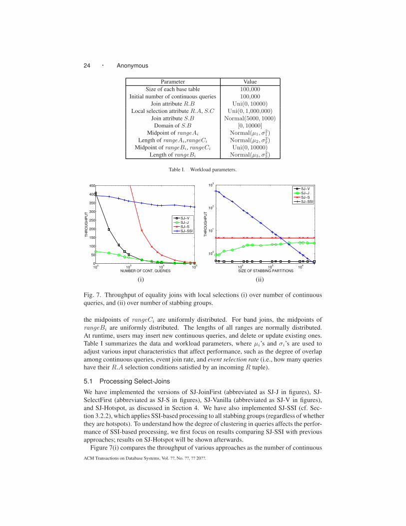
24 · Anonymous
Parameter Value
Size of each base table 100,000Initial number of continuous queries 100,000
Join attribute R.B Uni(0, 10000)Local selection attribute R.A, S.C Uni(0, 1,000,000)
Join attribute S.B Normal(5000, 1000)Domain of S.B [0, 10000]
Midpoint of rangeAi Normal(µ1, σ21)
Length of rangeAi,rangeCi Normal(µ2, σ22)
Midpoint of rangeBi, rangeCi Uni(0, 10000)Length of rangeBi Normal(µ3, σ
23)
Table I. Workload parameters.
102
103
104
105
0
50
100
150
200
250
300
350
400
450
NUMBER OF CONT. QUERIES
TH
RO
UG
HP
UT
SJ−V
SJ−J
SJ−S
SJ−SSI
102
103
104
100
101
102
103
SIZE OF STABBING PARTITIONS
TH
RO
UG
HP
UT
SJ−V
SJ−J
SJ−S
SJ−SSI
(i) (ii)
Fig. 7. Throughput of equality joins with local selections (i) over number of continuous
queries, and (ii) over number of stabbing groups.
the midpoints of rangeCi are uniformly distributed. For band joins, the midpoints of
rangeBi are uniformly distributed. The lengths of all ranges are normally distributed.
At runtime, users may insert new continuous queries, and delete or update existing ones.
Table I summarizes the data and workload parameters, where µi’s and σi’s are used to
adjust various input characteristics that affect performance, such as the degree of overlap
among continuous queries, event join rate, and event selection rate (i.e., how many queries
have their R.A selection conditions satisfied by an incoming R tuple).
5.1 Processing Select-Joins
We have implemented the versions of SJ-JoinFirst (abbreviated as SJ-J in figures), SJ-
SelectFirst (abbreviated as SJ-S in figures), SJ-Vanilla (abbreviated as SJ-V in figures),
and SJ-Hotspot, as discussed in Section 4. We have also implemented SJ-SSI (cf. Sec-
tion 3.2.2), which applies SSI-based processing to all stabbing groups (regardless of whether
they are hotspots). To understand how the degree of clustering in queries affects the perfor-
mance of SSI-based processing, we first focus on results comparing SJ-SSI with previous
approaches; results on SJ-Hotspot will be shown afterwards.
Figure 7(i) compares the throughput of various approaches as the number of continuous
ACM Transactions on Database Systems, Vol. ??, No. ??, ?? 20??.
Input-Sensitive Scalable Continuous Join Query Processing · 25
queries increases from 100 to 100,000. In this set of experiments, the stabbing number
for rangeCi is roughly 30; each incoming R tuple on average joins with 1000 S tuples.
In this figure, we see that SJ-Vanilla’s performance degrades linearly with the number of
continuous queries and therefore is not scalable at all. The average event selection rate
is 0.1; that is, an incoming R tuple satisfies the R.A selection conditions for 10% of all
continuous queries on average. Consequently, SJ-SelectFirst, which works by iterating
through queries whose R.A selection conditions are satisfied, performs well only when
the number of queries is small. Similar to SJ-Vanilla, its performance degrades linearly
with the number of queries. The performance degradation of SJ-JoinFirst can be attributed
to higher cost in two-dimensional point stabbing queries; in our experiments we used R-
trees to support these queries. Although the performance of SJ-JoinFirst does not drop as
drastically as SJ-SelectFirst and SJ-Vanilla, its throughput is less than 5% of SJ-SSI in the
case of 100,000 queries.
Compared with the other approaches, SJ-SSI demonstrates excellent scalability. Its
throughput only drops by less than 20% when the number of queries increases from 100to 100,000. The reason is that SJ-SSI depends primarily on the number of stabbing groups
rather than the number of queries. As long as the number of groups is stable (roughly 30 for
these experiments), SJ-SSI’s performance is relatively stable. The slight performance drop
comes from the increasing cost of the point stabbing query within each stabbing group,
because each group on average contains more queries.
Figure 7(ii) compares the performance of various approaches over a range of clustered-
ness among rangeCi’s. The number of continuous queries stays at 100,000, but we in-
crease the number of stabbing groups by decreasing mean and variance of interval lengths.
As can be seen, SJ-Vanilla and SJ-SelectFirst are completely indifferent to the clustered-
ness of queries, while SJ-SSI benefits from smaller numbers of stabbing groups. SJ-
SelectFirst outperforms SJ-SSI when there are roughly more than 2000 stabbing groups,
as the event selection rate is roughly 250 queries in these experiments. In the worse case,
when all query ranges are disjoint, SJ-SSI degenerates to SJ-Vanilla. As a side note, it is
interesting that SJ-JoinFirst performs better on less clustered queries. The reason is that
the cost of querying an R-tree tends to be lower if the indexed objects overlap less.
Figure 8(i) shows the throughput of SJ-SelectFirst and SJ-SSI when we decrease the
average event selection rate (SJ-JoinFirst and SJ-Vanilla are unaffected by this parameter).
We control this rate by fine-tuning the distribution of rangeAi’s. From this figure, we see
that SJ-SelectFirst is very sensitive to this rate. Its throughput deteriorates linearly, since
this rate directly controls how large n′ is in Theorem 3). On the other hand, SJ-SSI is
unaffected.
Figure 8(ii) studies the impact of event join rate, i.e., how many S tuples join with the
incoming event. We control increase this rate by fine-tuning the distribution of S.B. Except
for SJ-JoinFirst, all other approaches are immune to increase in this rate. SJ-JoinFirst’s
performance degrades linearly as the number of intermediate join result tuples increases.
In previous experiments, we have only considered SJ-SSI, which applies SSI-based pro-
cessing to all stabbing groups. Now, we conduct experiments to demonstrate the effective-
ness of SJ-Hotspot, which selectively applies SSI-based processing to hotspots. To better
control these experiments, we generate workloads differently from the previous experi-
ments. Each workload consists of 500,000 queries, whose degree of clusteredness varies
across workloads. We set α = 0.1% for SJ-Hotspot; i.e., each hotspot contains at least 500
ACM Transactions on Database Systems, Vol. ??, No. ??, ?? 20??.

26 · Anonymous
50 100 150 200 250 300 350 400 450 5000
100
200
300
400
500
600
700
800
900
1000
AVERAGE EVENT SELECTION RATE
TH
RO
UG
HP
UT
SJ−S
SJ−SSI
101
102
103
104
1
10
100
1000
AVERAGE EVENT JOIN RATE
TH
RO
UG
HP
UT
SJ−V
SJ−J
SJ−S
SJ−SSI
(i) (ii)
Fig. 8. Throughput of equality joins with local selections (i) over event selection rate (the
number of queries whose R.A selection conditions are satisfied by the incoming tuple),
and (ii) over event join rate (the number of S tuples that join with the incoming tuple).
queries. We vary the fraction of queries that belong to hotspots by setting the target per-
centages between 10% and 100%, in increments of 10%. For each target percentage p, we
generate 500,000×p queries by drawing the midpoints and lengths of their rangeCi’s both
from normal distributions, such that most of these queries belong to α-hotspots. Not all
of them do; as can be seen from Figure 9, the actual percentages shown on the horizontal
axis are always slightly lower than the corresponding target percentages. We then generate
the remaining queries by drawing their interval midpoints uniformly from a range disjoint
from the hotspots, and drawing their interval lengths from a normal distribution, such that
these intervals form a large number of small groups.
Because of the larger workloads, experiments in this set were conducted on a Linux
machine with a 2.13GHz Intel dual-core processor and 2GB of memory. In Figure 9, we
compare three approaches: SJ-SelectFirst, SJ-SSI, and SJ-Hotspot (using SJ-SelectFirst
on scattered queries). SJ-SelectFirst, unable to exploit the clusteredness among queries,
behaves nearly identically across workloads. Between SJ-SelectFirst and SJ-SSI, there
is no clear winner: SJ-SSI is better when queries are more clustered, but suffers from
large numbers of small stabbing groups when queries are scattered. On the other hand, the
performance of SSJ-Hotspot improves linearly with the increasing coverage by hotspots, as
it benefits from the ability of SSI-based processing in exploiting clusteredness for efficient
group processing. Moreover, by restricting SSI-based processing to hotspots, SJ-Hotspot is
able to avoid going through a large number of small stabbing groups, where SJ-SSI suffers.
5.2 Processing Band Joins
In this set of experiments, we study the performance of our SSI-based approach for con-
tinuous band joins. We compare BJ-SSI with BJ-DOuter (abbreviated as BJ-D in figures),
BJ-QOuter (abbreviated as BJ-Q in figures), and BJ-MJ, discussed in Section 3.1. Again,
to focus our attention on the effectiveness of SSI-based processing itself, we show results
of BJ-SSI without the hotspot optimization.
Figure 10(i) shows the throughput of various approaches over an increasing number of
continuous queries from 50 to 500,000. As the number of queries increases, the number
ACM Transactions on Database Systems, Vol. ??, No. ??, ?? 20??.
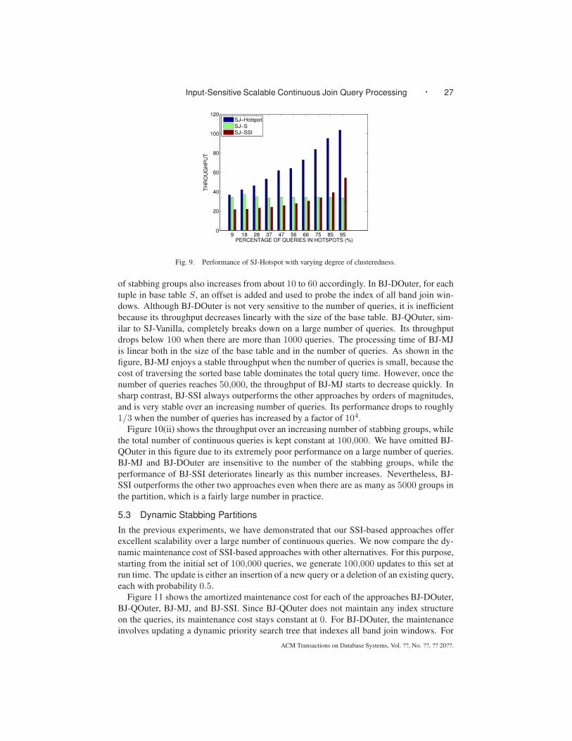
Input-Sensitive Scalable Continuous Join Query Processing · 27
9 18 28 37 47 56 66 75 85 950
20
40
60
80
100
120
PERCENTAGE OF QUERIES IN HOTSPOTS (%)
TH
RO
UG
HP
UT
SJ−Hotspot
SJ−S
SJ−SSI
Fig. 9. Performance of SJ-Hotspot with varying degree of clusteredness.
of stabbing groups also increases from about 10 to 60 accordingly. In BJ-DOuter, for each
tuple in base table S, an offset is added and used to probe the index of all band join win-
dows. Although BJ-DOuter is not very sensitive to the number of queries, it is inefficient
because its throughput decreases linearly with the size of the base table. BJ-QOuter, sim-
ilar to SJ-Vanilla, completely breaks down on a large number of queries. Its throughput
drops below 100 when there are more than 1000 queries. The processing time of BJ-MJ
is linear both in the size of the base table and in the number of queries. As shown in the
figure, BJ-MJ enjoys a stable throughput when the number of queries is small, because the
cost of traversing the sorted base table dominates the total query time. However, once the
number of queries reaches 50,000, the throughput of BJ-MJ starts to decrease quickly. In
sharp contrast, BJ-SSI always outperforms the other approaches by orders of magnitudes,
and is very stable over an increasing number of queries. Its performance drops to roughly
1/3 when the number of queries has increased by a factor of 104.
Figure 10(ii) shows the throughput over an increasing number of stabbing groups, while
the total number of continuous queries is kept constant at 100,000. We have omitted BJ-
QOuter in this figure due to its extremely poor performance on a large number of queries.
BJ-MJ and BJ-DOuter are insensitive to the number of the stabbing groups, while the
performance of BJ-SSI deteriorates linearly as this number increases. Nevertheless, BJ-
SSI outperforms the other two approaches even when there are as many as 5000 groups in
the partition, which is a fairly large number in practice.
5.3 Dynamic Stabbing Partitions
In the previous experiments, we have demonstrated that our SSI-based approaches offer
excellent scalability over a large number of continuous queries. We now compare the dy-
namic maintenance cost of SSI-based approaches with other alternatives. For this purpose,
starting from the initial set of 100,000 queries, we generate 100,000 updates to this set at
run time. The update is either an insertion of a new query or a deletion of an existing query,
each with probability 0.5.
Figure 11 shows the amortized maintenance cost for each of the approaches BJ-DOuter,
BJ-QOuter, BJ-MJ, and BJ-SSI. Since BJ-QOuter does not maintain any index structure
on the queries, its maintenance cost stays constant at 0. For BJ-DOuter, the maintenance
involves updating a dynamic priority search tree that indexes all band join windows. For
ACM Transactions on Database Systems, Vol. ??, No. ??, ?? 20??.
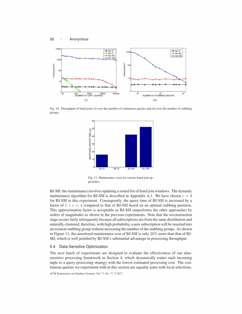
28 · Anonymous
50 500 5000 50000 5000001
10
100
1000
10000
NUMBER OF CONT. QUERIES
TH
RO
UG
HP
UT
BJ−D
BJ−Q
BJ−MJ
BJ−SSI
102
103
104
1
10
100
1000
NUMBER OF STABBING GROUPS
TH
RO
UG
HP
UT
BJ−D
BJ−MJ
BJ−SSI
(i) (ii)
Fig. 10. Throughput of band-joins (i) over the number of continuous queries and (ii) over the number of stabbing
groups.
BJ−D BJ−Q BJ−MJ BJ−SSI0
10
20
30
40
50
60
AM
OR
TIZ
ED
UP
DA
TE
TIM
E (
µs)
Fig. 11. Maintenance costs for various band-join ap-
proaches.
BJ-MJ, the maintenance involves updating a sorted list of band join windows. The dynamic
maintenance algorithm for BJ-SSI is described in Appendix A.1. We have chosen ε = 3for BJ-SSI in this experiment. Consequently, the query time of BJ-SSI is increased by a
factor of 1 + ε = 4 compared to that of BJ-SSI based on an optimal stabbing partition.
This approximation factor is acceptable as BJ-SSI outperforms the other approaches by
orders of magnitudes as shown in the previous experiments. Note that the reconstruction
stage occurs fairly infrequently because all subscriptions are from the same distribution and
naturally clustered; therefore, with high probability, a new subscription will be inserted into
an existent stabbing group without increasing the number of the stabbing groups. As shown
in Figure 11, the amortized maintenance cost of BJ-SSI is only 20% more than that of BJ-
MJ, which is well justified by BJ-SSI’s substantial advantage in processing throughput.
5.4 Data-Sensitive Optimization
The next batch of experiments are designed to evaluate the effectiveness of our data-
sensitive processing framework in Section 4, which dynamically routes each incoming
tuple to a query processing strategy with the lowest estimated processing cost. The con-
tinuous queries we experiment with in this section are equality joins with local selections.
ACM Transactions on Database Systems, Vol. ??, No. ??, ?? 20??.

Input-Sensitive Scalable Continuous Join Query Processing · 29
Processing strategy Parameter Value, 95% confidence interval
SJ-JoinFirst αJ 0.25, [0.24, 0.26]δJ 4.34, [4.23, 4.44]
SJ-SelectFirst αS 0.64, [0.63, 0.65]βS 42.49, [35.06, 49.92]γS 1.19, [1.16, 1.22]
SJ-Vanilla αV 0.36, [0.33, 0.38]γV 0.17, [0.15, 0.20]
SJ-Hotspot αH 0.19, [0.19, 0.20]βH 70.19, [50.49, 89.89]γH 1.17, [1.14, 1.21]δH 0.08, [0.06, 0.10]
Table II. Fitted parameters in cost models.
We refer to our data-sensitive approach as SJ-Dynamic. The quantities m′, n′, and n′′
needed in evaluating cost formulas are estimated at runtime using histograms, as described
in Section 4. For our experiments, we simply use standard equi-width histograms with 100buckets, which turn out to be sufficient in making reasonably good optimization decisions.
We first conduct parameter fitting for the cost models as described in Section 4. In par-
ticular, to collect training data for parameter fitting, we vary the number of queries from
100,000 to 500,000 (in increments of 100,000), and vary the number of tuples in S from
100,000 to 500,000 (in increments of 100,000); for each combination we generate 1000 in-
coming R tuples and separately measure each component cost for all processing strategies.
After collecting all training data, we use standard linear regression to fit the parameters
individually. Table II shows the least squares fit of all parameters and the associated 95%confidence intervals.
We compare SJ-Dynamic with four static strategies SJ-JoinFirst, SJ-SelectFirst, SJ-
Vanilla, and SJ-Hotpot, where a single processing strategy is applied to all incoming tuples.
In addition, we also compare SJ-Dynamic with an oracle algorithm, SJ-Optimum, which
always chooses one of SJ-JoinFirst, SJ-SelectFirst, SJ-Vanilla, and SJ-Hotpot with the
lowest actual processing cost for each incoming tuple. Note SJ-Optimum is impossible to
attain in practice; we obtain the choice of SJ-Optimum only after running all four available
strategies.
Figure 12 compares the throughput of different processing strategies. Labels on the
horizontal axis indicate the workload size (in thousands); 100 means a workload consisting
of 100,000 queries and an S table with 100,000 tuples. From Figure 12, we can see that
among the static strategies, SJ-Hotspot performs much better than the others (by more than
a factor of 3). However, it is evident that SJ-Hotspot is not always the best strategy for every
incoming tuple, because its throughput is still much less than that of SJ-Optimum. For
example, when there are 100,000 queries and 100,000 S tuples, throughput of SJ-Hotspot
is only less than 50% of SJ-Optimum. SJ-Dynamic is able to achieve higher throughput
than SJ-Hotspot in all workloads since it chooses the most promising processing strategy
on the fly. In some cases, SJ-dynamic beats SJ-Hotspot by more than 50%.
Figure 13 shows the breakdown of runtime choices made by SJ-Dynamic. Roughly,
more than 70% of the incoming tuples are processed using SJ-Hotspot; SJ-SelectFirst and
SJ-JoinFirst are chosen for 25% and 5% of the tuples respectively; SJ-Vanilla is never
chosen, even for the smallest workload.
ACM Transactions on Database Systems, Vol. ??, No. ??, ?? 20??.
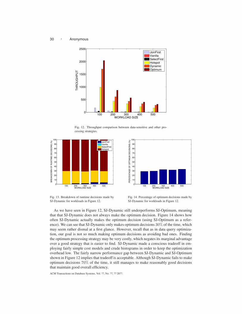
30 · Anonymous
100 200 300 400 5000
500
1000
1500
2000
2500
TH
RO
UG
HP
UT
WORKLOAD SIZE
JoinFirst
Vanilla
SelectFirst
Hotspot
Dynamic
Optimum
Fig. 12. Throughput comparison between data-sensitive and other pro-
cessing strategies.
100 200 300 400 5000
10
20
30
40
50
60
70
80
90
100
BR
EA
KD
OW
N O
F R
UN
TIM
E D
EC
ISIO
NS
(%
)
WORKLOAD SIZE
JoinFirst
Vanilla
SelectFirst
Hotspot
Fig. 13. Breakdown of runtime decisions made by
SJ-Dynamic for workloads in Figure 12.
100 200 300 400 5000
10
20
30
40
50
60
70
80
90
100
PE
RC
EN
TA
GE
OF
OP
TIM
UM
DE
CIS
ION
S (
%)
WORKLOAD SIZE
Fig. 14. Percentage of optimum decisions made by
SJ-Dynamic for workloads in Figure 12.
As we have seen in Figure 12, SJ-Dynamic still underperforms SJ-Optimum, meaning
that that SJ-Dynamic does not always make the optimum decision. Figure 14 shows how
often SJ-Dynamic actually makes the optimum decision (using SJ-Optimum as a refer-
ence). We can see that SJ-Dynamic only makes optimum decisions 30% of the time, which
may seem rather dismal at a first glance. However, recall that as in data query optimiza-
tion, our goal is not so much making optimum decisions as avoiding bad ones. Finding
the optimum processing strategy may be very costly, which negates its marginal advantage
over a good strategy that is easier to find. SJ-Dynamic made a conscious tradeoff in em-
ploying fairly simple cost models and crude histograms in order to keep the optimization
overhead low. The fairly narrow performance gap between SJ-Dynamic and SJ-Optimum
shown in Figure 12 implies that tradeoff is acceptable. Although SJ-Dynamic fails to make
optimum decisions 70% of the time, it still manages to make reasonably good decisions
that maintain good overall efficiency.
ACM Transactions on Database Systems, Vol. ??, No. ??, ?? 20??.
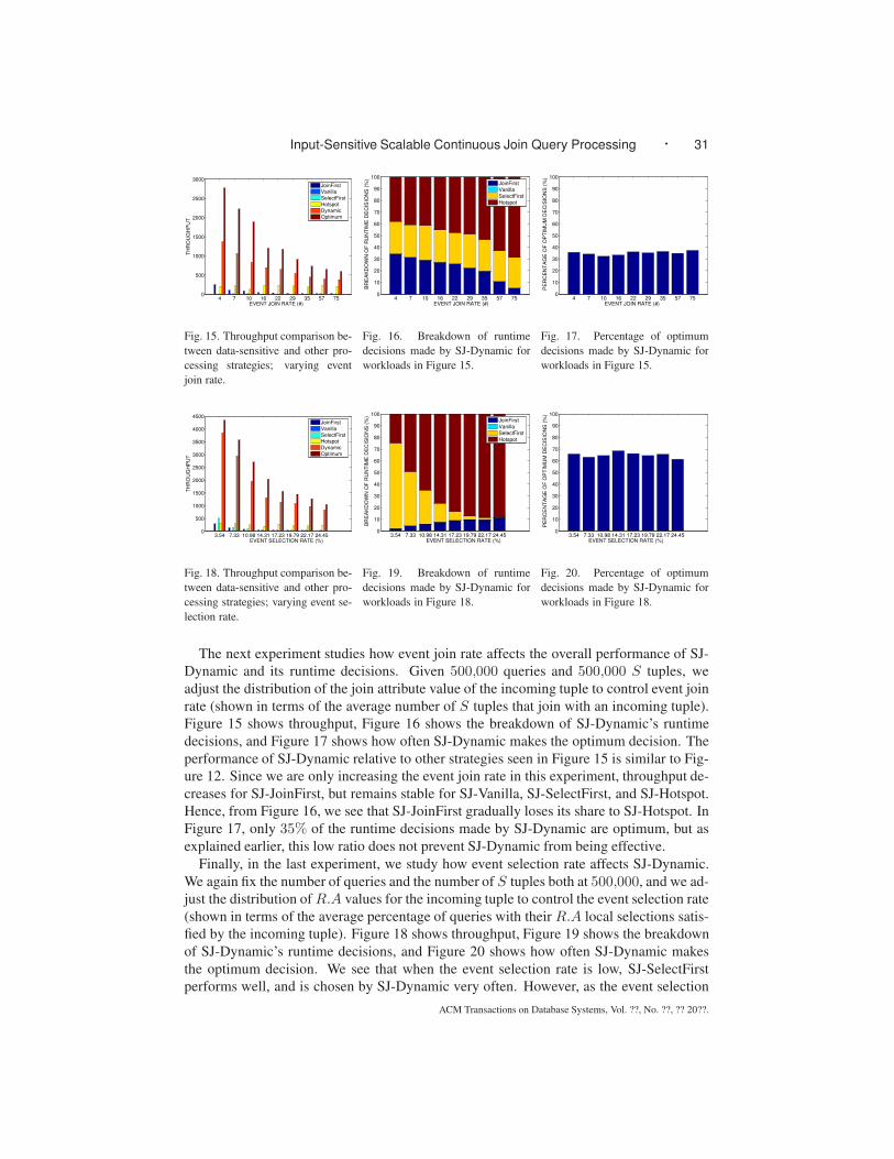
Input-Sensitive Scalable Continuous Join Query Processing · 31
4 7 10 16 22 29 35 57 750
500
1000
1500
2000
2500
3000
TH
RO
UG
HP
UT
EVENT JOIN RATE (#)
JoinFirst
Vanilla
SelectFirst
Hotspot
Dynamic
Optimum
Fig. 15. Throughput comparison be-
tween data-sensitive and other pro-
cessing strategies; varying event
join rate.
4 7 10 16 22 29 35 57 750
10
20
30
40
50
60
70
80
90
100
BR
EA
KD
OW
N O
F R
UN
TIM
E D
EC
ISIO
NS
(%
)
EVENT JOIN RATE (#)
JoinFirst
Vanilla
SelectFirst
Hotspot
Fig. 16. Breakdown of runtime
decisions made by SJ-Dynamic for
workloads in Figure 15.
4 7 10 16 22 29 35 57 750
10
20
30
40
50
60
70
80
90
100
PE
RC
EN
TA
GE
OF
OP
TIM
UM
DE
CIS
ION
S (
%)
EVENT JOIN RATE (#)
Fig. 17. Percentage of optimum
decisions made by SJ-Dynamic for
workloads in Figure 15.
3.54 7.33 10.98 14.31 17.23 19.79 22.17 24.450
500
1000
1500
2000
2500
3000
3500
4000
4500
TH
RO
UG
HP
UT
EVENT SELECTION RATE (%)
JoinFirst
Vanilla
SelectFirst
Hotspot
Dynamic
Optimum
Fig. 18. Throughput comparison be-
tween data-sensitive and other pro-
cessing strategies; varying event se-
lection rate.
3.54 7.33 10.98 14.31 17.23 19.79 22.17 24.450
10
20
30
40
50
60
70
80
90
100
BR
EA
KD
OW
N O
F R
UN
TIM
E D
EC
ISIO
NS
(%
)
EVENT SELECTION RATE (%)
JoinFirst
Vanilla
SelectFirst
Hotspot
Fig. 19. Breakdown of runtime
decisions made by SJ-Dynamic for
workloads in Figure 18.
3.54 7.33 10.98 14.31 17.23 19.79 22.17 24.450
10
20
30
40
50
60
70
80
90
100
PE
RC
EN
TA
GE
OF
OP
TIM
UM
DE
CIS
ION
S (
%)
EVENT SELECTION RATE (%)
Fig. 20. Percentage of optimum
decisions made by SJ-Dynamic for
workloads in Figure 18.
The next experiment studies how event join rate affects the overall performance of SJ-
Dynamic and its runtime decisions. Given 500,000 queries and 500,000 S tuples, we
adjust the distribution of the join attribute value of the incoming tuple to control event join
rate (shown in terms of the average number of S tuples that join with an incoming tuple).
Figure 15 shows throughput, Figure 16 shows the breakdown of SJ-Dynamic’s runtime
decisions, and Figure 17 shows how often SJ-Dynamic makes the optimum decision. The
performance of SJ-Dynamic relative to other strategies seen in Figure 15 is similar to Fig-
ure 12. Since we are only increasing the event join rate in this experiment, throughput de-
creases for SJ-JoinFirst, but remains stable for SJ-Vanilla, SJ-SelectFirst, and SJ-Hotspot.
Hence, from Figure 16, we see that SJ-JoinFirst gradually loses its share to SJ-Hotspot. In
Figure 17, only 35% of the runtime decisions made by SJ-Dynamic are optimum, but as
explained earlier, this low ratio does not prevent SJ-Dynamic from being effective.
Finally, in the last experiment, we study how event selection rate affects SJ-Dynamic.
We again fix the number of queries and the number of S tuples both at 500,000, and we ad-
just the distribution of R.A values for the incoming tuple to control the event selection rate
(shown in terms of the average percentage of queries with their R.A local selections satis-
fied by the incoming tuple). Figure 18 shows throughput, Figure 19 shows the breakdown
of SJ-Dynamic’s runtime decisions, and Figure 20 shows how often SJ-Dynamic makes
the optimum decision. We see that when the event selection rate is low, SJ-SelectFirst
performs well, and is chosen by SJ-Dynamic very often. However, as the event selection
ACM Transactions on Database Systems, Vol. ??, No. ??, ?? 20??.

32 · Anonymous
rate increases, SJ-SelectFirst becomes increasingly unfavored by SJ-Dynamic, which in-
tuitively makes sense. We also see that SJ-Dynamic often does not make the optimum
decision; nevertheless, SJ-Dynamic still dramatically outperforms any of the static pro-
cessing strategies.
6. RELATED WORK
As mentioned in Section 1, scalable continuous query processing plays a pivotal role in
many applications (e.g., [Widom and Ceri 1996; Hanson et al. 1999; Carney et al. 2002;
Special 2003]). For example, publish/subscribe systems [Liu et al. 1999; Chen et al. 2000;
Pereira et al. 2001; Dittrich et al. 2005; Demers et al. 2006] by definition need to handle a
huge number of subscriptions (continuous queries) efficiently.
Many continuous query and stream processing systems have been proposed (e.g., [Chen
et al. 2000; Madden et al. 2002; Chandrasekaran and Franklin 2003; Special 2003]). Ni-
agaraCQ [Chen et al. 2000] is able to group-process selections and share processing of
identical join operations. However, it cannot group process joins with different join con-
ditions (such as band joins). Moreover, NiagaraCQ groups selections and joins separately,
resulting in strategies similar to SJ-JoinFirst and SJ-SelectFirst, whose limitations were al-
ready discussed in Section 3. Our work is able to overcome these limitations. CACQ [Mad-
den et al. 2002] is a continuous query engine that leverages Eddies [Avnur and Hellerstein
2000] to route tuples adaptively to different operators on the fly. It is able to group-process
filters, and supports dynamic reordering of joins and filters. However, like NiagaraCQ,
it still does not support group processing of joins with different join conditions, and pro-
cesses selections and joins separately. PSoup [Chandrasekaran and Franklin 2003] treats
data and queries analogously, thereby making it possible to exploit set-oriented process-
ing on a group of joins with arbitrary join conditions. However, PSoup is not specific
on what efficient techniques to use for different types of join conditions. Its approach of
instantiating partially completed join queries implies time complexity linear in the num-
ber of queries. In contrast, our new approach can exploit clustering of queries to achieve
sublinear complexity. Like PSoup, [Lim et al. 2006] also recognizes the duality of data
and queries, and applies spatial join techniques to the problem of processing continuous
queries. While the proposed algorithm has additional features such as support for batching
and sliding windows, it essentially adopts a strategy similar to SJ-JoinFirst; our approach
can offer higher efficiency by exploiting data and query characteristics.
Cayuga [Demers et al. 2006] considers scalable processing of subscriptions expressed in
an event algebra, with constructs analogous to joins. Cayuga uses indexes extensively for
efficient group processing, but they are essentially predicate indexes. Although Cayuga’s
automata-based processing is not directly comparable to our work because of different
data models and query semantics, on a high level it resembles SJ-SelectFirst. Related
to Cayuga, there is a large body work on scalable XML event processing (e.g., XML
Toolkit [Green et al. 2004], YFilter [Diao et al. 2003], and XSCL [Hong et al. 2007]),
some of which also employed automata-based processing and query indexing.
[Agarwal et al. 2005] considered the problem of indexing continuous band-join queries,
and presented an indexing structure with subquadratic space and sublinear query time.
However, the structure is mainly of theoretical interest. [Agarwal et al. 2006] presented
data structures and algorithms for query-sensitive processing of continuous select-joins and
band joins, as well as histogram construction for intervals. This paper additionally studies
ACM Transactions on Database Systems, Vol. ??, No. ??, ?? 20??.

Input-Sensitive Scalable Continuous Join Query Processing · 33
window joins, proposes the data-sensitive processing framework, and presents experiments
demonstrating the power of combining data-sensitive, and query-sensitive processing in a
unified input-sensitive approach. This also contains more details, including full proofs and
the refined algorithm for maintaining stabbing partitions (Appendix A).
Related to data-sensitive processing, there has been extensive work on adaptive query
optimization (e.g., [Avnur and Hellerstein 2000; Markl et al. 2004; Bizarro et al. 2005]).
With the exception of CBR [Bizarro et al. 2005], most previous approaches use a single
plan for all almost all tuples at a given time. Some systems, such as Eddies [Avnur and
Hellerstein 2000], provides mechanisms for adapting the plan on an individual tuple basis,
but their policies typically do not result in plans that changes for every incoming tuple.
In CBR [Bizarro et al. 2005], each operator is profiled and learning techniques are used
to help choose query plan dynamically for each incoming tuple. In contrast, our data-
sensitive processing framework adopts a more conventional optimization approach using
more standard cost estimation and statistics collection techniques.
7. CONCLUSION AND FUTURE WORK
In this paper, we have presented a novel, input-sensitive approach to scalable continuous
query processing. The input sensitivity of our approach manifests in two ways. First, we
have developed query-sensitive data structures and algorithms that exploit the clustering
pattern in continuous queries in a principled manner for efficient group processing. Second,
we have developed a data-sensitive processing framework that makes runtime, cost-based
decisions on how to process each incoming tuple based on its characteristics. Together,
query-sensitive and data-sensitive techniques bring dramatic performance improvements
over existing methods for scalable continuous query processing.
Our work opens the door to many directions of future work. First, it would be interest-
ing to extend the idea of clustering by stabbing partition to multidimensional spaces, so
that we can better handle multi-attribute selection conditions. More generally, we plan to
investigate group processing for more complex queries, e.g., those combining both band-
join and local selection conditions, as well as possible aggregation. Although we have
taken the first step with this paper, it remains a challenging problem to develop methods
for composing group-processing techniques for more complex queries. Finally, this paper
assumes that we process one incoming tuple at at time. Batching has been shown to be
very effective in publish/subscribe and continuous query systems [Fischer and Kossmann
2005; He et al. 2005; Lim et al. 2006]. We plan to extend our approach to take advan-
tage of batching when possible. How to combine group processing of queries and batch
processing of tuples together effectively is an intriguing new challenge.
ACKNOWLEDGMENTS
Removed to ensure anonymity.
REFERENCES
AGARWAL, P. K., ARGE, L., BRODAL, G. S., AND VITTER, J. S. 1999. I/O-efficient dynamic point location in
monotone planar subdivisions. In Proc. of the 1999 ACM-SIAM Symposium on Discrete Algorithms. 11–20.
AGARWAL, P. K., XIE, J., YANG, J., AND YU, H. 2005. Monitoring continuous band-join queries over dynamic
data. In Proc. of the 16th Intl. Sympos. Algorithms and Computation. Spring-Verlag, Hanan, China, 349–359.
AGARWAL, P. K., XIE, J., YANG, J., AND YU, H. 2006. Scalable continuous query processing by tracking
hotspots. In Proc. of the 2006 Intl. Conf. on Very Large Data Bases. Seoul, Korea, 31–42.
ACM Transactions on Database Systems, Vol. ??, No. ??, ?? 20??.

34 · Anonymous
ARGE, L. AND VITTER, J. 2003. Optimal external memory interval management. SIAM J. Comput. 32, 6,
1488–1508.
AVNUR, R. AND HELLERSTEIN, J. M. 2000. Eddies: Continuously adaptive query processing. In Proc. of the
2000 ACM SIGMOD Intl. Conf. on Management of Data. ACM, Dallas, Texas, USA, 261–272.
BABU, S., BIZARRO, P., AND DEWITT, D. 2005. Proactive re-optimization. In Proc. of the 2005 ACM SIGMOD
Intl. Conf. on Management of Data. ACM, Baltimore, Maryland, USA.
BIZARRO, P., BABU, S., DEWITT, D., AND WIDOM, J. 2005. Robust query processing through progressive
optimization. In Proc. of the 2005 Intl. Conf. on Very Large Data Bases. VLDB, Trondheim, Norway.
CARNEY, D., CETINTEMEL, U., CHERNIACK, M., CONVEY, C., LEE, S., SEIDMAN, G., STONEBRAKER, M.,
TATBUL, N., AND ZDONIK, S. B. 2002. Monitoring streams - a new class of data management applications.
In Proc. of the 2002 Intl. Conf. on Very Large Data Bases. VLDB, Hongkong, China, 215–226.
CHANDRASEKARAN, S. AND FRANKLIN, M. J. 2003. Psoup: a system for streaming queries over streaming
data. VLDB Journal 12, 2, 140–156.
CHEN, J., DEWITT, D. J., TIAN, F., AND WANG, Y. 2000. NiagraCQ: A scalable continuous query system for
internet databases. In Proc. of the 2000 ACM SIGMOD Intl. Conf. on Management of Data. ACM, Dallas,
Texas, USA, 379–390.
DE BERG, M., VAN KREVELD, M., OVERMARS, M., AND SCHWARZKOPF, O. 2000. Computational Geometry:
Algorithms and Applications, 2nd ed. Springer, New York, USA.
DEMERS, A. J., GEHRKE, J., HONG, M., RIEDEWALD, M., AND WHITE, W. M. 2006. Towards expressive
publish/subscribe systems. In Proc. of the 2006 Intl. Conf. on Extending Database Technology. Munich,
Germany, 627–644.
DEWITT, D. J., NAUGHTON, J. F., AND SCHNEIDER, D. A. 1991. An evaluation of non-equijoin algorithms.
In Proc. of the 1991 Intl. Conf. on Very Large Data Bases. VLDB, Barcelona, Catalonia, Spain, 443–452.
DIAO, Y., ALTINEL, M., FRANKLIN, M. J., ZHANG, H., AND FISCHER, P. 2003. Path sharing and predicate
evaluation for high-performance XML filtering. ACM Trans. on Database Systems 28, 4, 467–516.
DITTRICH, J.-P., FISCHER, P. M., AND KOSSMANN, D. 2005. Agile: adaptive indexing for context-aware
information filters. In Proc. of the 2005 ACM SIGMOD Intl. Conf. on Management of Data. ACM, Baltimore,
Maryland, USA, 215–226.
DU, Q., FABER, V., AND GUNZBURGER, M. 1999. Centroidal Voronoi tessellations: Applications and algo-
rithms. SIAM Reviews 41, 637–676.
FISCHER, P. M. AND KOSSMANN, D. 2005. Batched processing for information filters. In Proc. of the 2005
Intl. Conf. on Data Engineering. Tokyo, Japan.
GEHRKE, J. AND HELLERSTEIN, J. M. 2004. Guest editorial to the special issue on data stream processing.
VLDB J. 13, 4, 317.
GREEN, T. J., GUPTA, A., MIKLAU, G., ONIZUKA, M., AND SUCIU, D. 2004. Processing XML streams with
deterministic automata and stream indexes. ACM Trans. on Database Systems 29, 4, 752–788.
HANSON, E. AND JOHNSON, T. 1991. The interval skip list: A data structure for finding all intervals that
overlap a point. In Proc. of the 1991 Workshop on Algorithms and Data Structures. Springer, Ottawa, Canada,
153–164.
HANSON, E. N., CARNES, C., HUANG, L., KONYALA, M., NORONHA, L., PARTHASARATHY, S., PARK, J. B.,
AND VERNON, A. 1999. Scalable trigger processing. In Proc. of the 1999 Intl. Conf. on Data Engineering.
IEEE Computer Society Press, Sydney, Austrialia, 266–275.
HAR-PELED, S. AND MAZUMDAR, S. 2004. Coresets for k-means and k-median clustering and their applica-
tions. In Proc. of the 2004 Annu. Sympos. Theory of Computing. ACM, Chicago, Illinois, USA, 291–300.
HE, H., XIE, J., YANG, J., AND YU, H. 2005. Asymmetric batch incremental view maintenance. In Proc. of
the 2005 Intl. Conf. on Data Engineering. Tokyo, Japan.
HONG, M., DEMERS, A. J., GEHRKE, J., KOCH, C., RIEDEWALD, M., AND WHITE, W. M. 2007. Massively
multi-query join processing in publish/subscribe systems. In Proc. of the 2007 ACM SIGMOD Intl. Conf. on
Management of Data. Beijing, China, 761–772.
IVES, Z., FLORESCU, D., FRIEDMAN, M., LEVY, A., AND WELD, D. 1999. An adaptive query execution
system for data integration. In Proc. of the 1999 ACM SIGMOD Intl. Conf. on Management of Data. ACM,
Philadelphia, Pennsylvania, USA.
ACM Transactions on Database Systems, Vol. ??, No. ??, ?? 20??.
Input-Sensitive Scalable Continuous Join Query Processing · 35
JAGADISH, H. V., KOUDAS, N., MUTHUKRISHNAN, S., POOSALA, V., SEVCIK, K., AND SUEL, T. 1998.
Optimal histograms with quality guarantees. In Proc. of the 1998 Intl. Conf. on Very Large Data Bases.
VLDB, New York City, USA, 275–286.
KATZ, M., NIELSEN, F., AND SEGAL, M. 2003. Maintenance of a piercing set for intervals with applications.
Algorithmica 36(1), 59–73.
KOUDAS, N., MUTHUKRISHNAN, S., AND SRIVASTAVA, D. 2000. Optimal histograms for hierarchical range
queries. In Proc. of the 2000 ACM Sympos. on Principles of Database Systems. ACM, Dallas, Texas, USA,
196–204.
LIM, H.-S., LEE, J.-G., LEE, M.-J., WHANG, K.-Y., AND SONG, I.-Y. 2006. Continuous query processing in
data streams using duality of data and queries. In Proc. of the 2006 ACM SIGMOD Intl. Conf. on Management
of Data. Chicago, Illinois, USA, 313–324.
LIU, L., PU, C., AND TANG, W. 1999. Continual queries for Internet scale event-driven information delivery.
IEEE Trans. on Knowledge and Data Engineering 11, 4, 610–628.
MADDEN, S., SHAH, M., HELLERSTEIN, J., AND RAMAN, V. 2002. Continuously adaptive continuous queries
over streams. In Proc. of the 2002 ACM SIGMOD Intl. Conf. on Management of Data. ACM, Madison,
Wisconsin, USA, 49–60.
MARKL, V., RAMAN, V., SIMMEN, D., LOHMAN, G., AND PIRAHESH, H. 2004. Robust query processing
through progressive optimization. In Proc. of the 2004 ACM SIGMOD Intl. Conf. on Management of Data.
Paris, France.
MCCREIGHT, E. M. 1985. Priority search trees. SIAM J. Comput. 14, 257–276.
PEREIRA, J., FABRET, F., JACOBSEN, H. A., LLIRBAT, F., AND SHASHA, D. 2001. Webfilter: A high-
throughput XML-based publish and subscribe system. In Proc. of the 2001 Intl. Conf. on Very Large Data
Bases. VLDB, Rome, Italy, 723–724.
Special 2003. Special issue on data stream processing. IEEE Data Eng. Bull. 26, 1.
TARJAN, R. E. 1983. Data Structures and Network Algorithms. Society for Industrial and Applied Mathematics,
Philadelphia, Pennsylvania, USA.
VAISHNAVI, V. K. 1982. Computing point enclosures. IEEE Trans. Computers 31, 1, 22–29.
WIDOM, J. AND CERI, S. 1996. Active Database Systems: Triggers and Rules For Advanced Database Pro-
cessing. Morgan Kaufmann, San Fransisco, California, USA.
A. DYNAMIC STABBING PARTITIONS
This section is devoted to an efficient implementation of Lemma 2. Because it is not a
prerequisite for understanding other parts of this paper, this section can be skipped at the
reader’s discretion.
We first observe that if one were to maintain the smallest stabbing partition of I (such
as the canonical stabbing partition) as intervals are inserted or deleted, then the stabbing
partition of I may completely change after a small constant number of insertions or dele-
tions. (A simple example is omitted for brevity.) Thus, we resort to a stabbing partition
of approximately smallest size. More precisely, we want to maintain a partition of size at
most (1 + ε)τ(I) for some parameter ε > 0, where recall that τ(I) is the size of the small-
est stabbing partition of I . Although the quality of the stabbing partition is compromised,
the benefit of resorting to an approximation is that the cost required for maintaining such a
relaxed partition is much lower than for maintaining the smallest one.
Typically we choose ε to be a small constant. The value of ε can be used as a tunable
parameter to achieve flexible tradeoffs between the quality of the stabbing partition and the
maintenance cost: a smaller ε results in a better stabbing partition, but also increases the
maintenance cost. Next we describe in detail how to maintain the stabbing partitions.
ACM Transactions on Database Systems, Vol. ??, No. ??, ?? 20??.

36 · Anonymous
A.1 A Simple Strategy
We sketch a lazy maintenance strategy that guarantees the quality of the stabbing partition.
It is very easy to implement and works reasonably well in practice, but may perform poorly
in the worst case.
Let I be a set of n intervals, and ε > 0 be a fixed positive parameter. The lazy strategy
works as follows. We begin with the canonical stabbing partition I of I of size τ0 = τ(I)as well as a corresponding stabbing set P . When a new interval γ is inserted into I , we
simply pick a point pγ ∈ γ and let P = P ∪ pγ; we also create a singleton group γand add it to I. When an interval γ is deleted from I , suppose that γ belongs to some
group Ii ∈ I. We then remove γ from Ii, and if Ii becomes empty after the removal
of γ, we also remove Ii from I and the stabbing point of Ii from P . After ετ0/(ε + 2)number of insertions and deletions, we trigger a reconstruction stage: we use Lemma 1 to
reconstruct the canonical stabbing partition (whose size is τ(I)) for the current I , which
takes O(n log n) time.
LEMMA 3. The above procedure maintains a stabbing partition of size at most (1 +ε)τ(I) at all times.
PROOF. Suppose this procedure maintains a stabbing partition I with size P . Then
P ≤ (1+ εε+2 )τ0 at all times, because each insertion increases the size of I by at most one,
and each deletion does not increase the size of I. On the other hand, note that inserting an
interval into I does not decrease τ(I), and deleting an interval from I may decrease τ(I)by at most one. Therefore τ(I) ≥ (1− ε
ε+2 )τ0 at any time before the reconstruction stage.
Hence,
P ≤ (1 +ε
ε + 2)τ0 = (1 + ε)(1 − ε
ε + 2)τ0 ≤ (1 + ε)τ(I)
This implies that the procedure always maintains a stabbing partition of size at most (1 +ε)τ(I).
The above strategy can be improved in several ways. For example, for a newly inserted
interval γ, if there already exists a point pi in the current stabbing set that stabs γ, and
suppose pi is the stabbing point for the group Ii, then we can simply add γ into Ii, instead
of creating a new singleton group γ in the stabbing partition. A more careful imple-
mentation would maintain the common intersection of each group, instead of just a single
stabbing point. For each new insertion γ, we check whether there exists a group whose
common intersection overlaps with γ, and if so, add γ to that group.
The condition for triggering a reconstruction stage (i.e., when the total number of in-
sertions and deletions reaches ετ0/(ε + 2)) can also be relaxed. Let I denote the set of
intervals after the last reconstruction and τ0 = τ(I). Suppose that m intervals have been
deleted from I so far since the last reconstruction (the total number of deletions so far
could be larger because some intervals may be inserted and subsequently deleted), then we
invoke a reconstruction stage only if |P | ≥ (1 + ε)(τ0 − m), where |P | is the size of the
maintained stabbing set at that time. Note that it is weaker than the old trigger condition,
and hence leads to less frequent invocations of reconstruction stages.
A.2 A Refined Algorithm
The amortized cost per insertion and deletion in the simple strategy above is O(n log n/(ετ0)).Katz et al. [Katz et al. 2003] presented a faster algorithm for maintaining the stabbing
ACM Transactions on Database Systems, Vol. ??, No. ??, ?? 20??.
Input-Sensitive Scalable Continuous Join Query Processing · 37
partition with O((1/ε) log n) worst-case amortized cost per insertion and deletion. The
drawback of their algorithm is that each insertion and deletion requires to update Ω(1/ε)groups in the stabbing partition. We present a similar algorithm with the same amortized
cost, but each insertion and deletion only requires to update one group in the stabbing parti-
tion. Recall that changes in the stabbing partition often need to be propagated to other data
structures associated with SSI at runtime. Our implementation therefore requires much
less frequent propagations and is more suitable for real-time applications.
Next we describe the algorithm in detail. Let P = p1, . . . , pτ0 be the stabbing set of I
returned by the greedy algorithm (Lemma 1), and let I = Ii | 1 ≤ i ≤ τ0 be the stabbing
partition of I corresponding to P . For each Ii ∈ I, we construct a height-balanced binary
tree Ti that supports each of INSERT, DELETE, SPLIT, and JOIN operations in O(log n)time [Tarjan 1983]. The leaves of Ti store the intervals of Ii from left to right in increasing
order of the left endpoints of intervals in Ii. Each internal node v of Ti with w and z as its
two children stores an interval γv = γw ∩ γz . Note that⋂
Ii, the common intersection of
all the intervals in Ii, is stored at the root of Ti.
We handle each newly inserted interval γ by picking a point pγ ∈ γ and letting P =P ∪ pγ, and adding a singleton group Iγ = γ into I.6 Let J be the set of intervals
inserted since the last reconstruction of the stabbing partition. Note that these intervals
appear as singleton sets in I. When an interval γ is deleted, we first check whether γ ∈ J .
If γ ∈ J , we simply remove pγ from P , γ from J , and γ from I. Otherwise we find Ii
such that γ ∈ Ii, and delete γ from Ii and the tree Ti; we discard Ii and Ti if Ii becomes
empty. Thus each insertion or deletion takes O(log n) time, and affects at most one group
in the stabbing partition.
After we have performed ετ0/(ε + 2) updates, we recompute the optimal stabbing set
of I , as well as a corresponding partition of I and the tree structure for each group in the
partition, by a reconstruction stage that emulates the greedy algorithm for computing an
optimal stabbing partition (Lemma 1). It outputs exactly the same stabbing set and partition
of I as the greedy algorithm. However, instead of examining each interval of I explicitly,
which would require O(n) time after sorting, it examines each of the O(τ0) groups in I,
in O(log n) time per group, thereby reducing the running time to O(τ0 log n). Complete
pseudo-code of the reconstruction stage is listed in Figure 21.
Throughout the reconstruction, we have the following invariant:
(⋆) For any γ ∈ Ii and ξ ∈ Ij with i < j, the left endpoint of ξ lies to the right of the left
endpoint of γ.
This invariant holds at the start of the reconstruction stage, because it clearly holds for the
initial partition of I computed by the greedy algorithm, and during subsequent updates,
intervals are only removed from but never added into each Ii. During the reconstruction
stage, the invariant will remain valid because of the same reason.
Let L1, L2, . . . be the sets in I = Ii | 1 ≤ i ≤ τ0 ∪ Iγ | γ ∈ J in increasing
order of the left endpoints of their respective common intersections. The reconstruction
procedure processes the sets L1, L2, . . . one by one, and outputs a new stabbing set and
6Again, this can be improved as in the simple strategy. If γ is already stabbed by some point p ∈ P , and suppose
that p is the leftmost such point in P , we can simply add γ to the group whose stabbing point is p. The choice
of such p is for maintaining the invariant (⋆) to be stated shortly. For simplicity, we refrain from involving this
refinement in our subsequent discussions.
ACM Transactions on Database Systems, Vol. ??, No. ??, ?? 20??.

38 · Anonymous
Algorithm RECONSTRUCTIONSTAGE
Input: Ii | i ≥ 1 ∪ Iγ | γ ∈ A (sorted), Ti for each Ii.
Output: smallest stabbing set P , a corresponding stabbing partition I of I , the tree structure TJ for each J ∈ I.
1: P, I← ∅; U, V, TU ← ∅;The collection of all intervals in the sets of U or V is denoted by J
2: while ∃ unprocessed nonempty groups do
3: K ← next unprocessed nonempty group;
4: Mark K processed;
5: if l(K) ≤ r(T
J) then
6: if K = Iγ for some γ ∈ A then
7: V ← V ∪ γ;8: else K = Ii for some 1 ≤ i ≤ τ09: I′i, Ii ← SPLIT(Ii, r(
T
J));
10: T′
i, Ti ← SPLIT(Ti, r(T
J));
11: U ← U ∪ I′i, TU ← JOIN(TU , T′
i);
12: Re-mark Ii unprocessed if Ii 6= ∅;13: else l(K) > r(
T
J)14: if K = Iγ for some γ ∈ A then
15: Ii ← next unprocessed nonempty group in Ij | 1 ≤ j ≤ τ0;16: I′i, Ii ← SPLIT(Ii, r(
T
J));
17: T′
i, Ti ← SPLIT(Ti, r(T
J));
18: U ← U ∪ I′i, TU ← JOIN(TU , T′
i);
19: TJ ← TU ;
20: for every γ ∈ V do
21: INSERT(TJ , γ);
22: I← I∪ J, P ← P ∪ r(T
J);23: if K = Iγ for some γ ∈ A then
24: U, TU ← ∅, V ← γ;25: else K = Ii for some 1 ≤ i ≤ τ026: U ← Ii, TU ← Ti, V ← ∅;
Fig. 21. Pseudo-code for the reconstruction stage.
the corresponding new group of I as well as the binary tree structure for each group in
the partition. During the process, it maintains a set A of active intervals, whose common
intersection γA =⋂
A is nonempty. Intuitively, the active set A consists of a set of
intervals on the frontier of this process, but has not yet formed a complete group because
more intervals might be added into it later. Note that for a reason that will become clear
shortly, we do not maintain A explicitly, but represent A as a family of subsets of sets in I.
Initially we set A = L1 and start processing L2. Suppose we have processed L1, . . . , Lu,
and returned q1, . . . , qx as stabbing points and the corresponding groups Q1, . . . , Qx. We
now process Lu+1. Let γu+1 =⋂
Lu+1, which is stored at the root of the binary tree for
Lu+1. There are two cases to consider.
Case 1: γA ∩ γu+1 6= ∅, i.e., all intervals in Lu+1 intersect rA. We add Lu+1 to A, set
γA = γA ∩ γu+1, and process Lu+2; see Figure 22.
Case 2: γA ∩ γu+1 = ∅. If Lu+1 ∈ Iγ | γ ∈ J, we let L be the leftmost unprocessed
group in Ii | 1 ≤ i ≤ τ0 (Figure 23 (a)); otherwise we set L = Lu+1 (Figure 23 (b)). Let
L′ be the subset of intervals in L whose left endpoints lie to the left of the right endpoint
of γA. We split L into two sets L′ and (new) L = L \ L′; we also split the binary tree
ACM Transactions on Database Systems, Vol. ??, No. ??, ?? 20??.

Input-Sensitive Scalable Continuous Join Query Processing · 39
A
Lu+1
A
γAγA
Fig. 22. Case 1: γA ∩ γu+1 6= ∅. Intervals in A are solid, and intervals in Lu+1 are dashed. We add Lu+1 to
A.
structure TL for L into TL′ and (new) TL accordingly. Note that the left endpoint of⋂
Lremains the same. We add L′ to A and set γA = γA∩γ′. Note that by (⋆), no other interval
from⋃
i≥u+1 Li can be added into A such that⋂
A remains nonempty. We then output a
new stabbing point qx+1 to be the right endpoint of γA and output a new group Qx+1 = A.
We need to construct the tree TQx+1for Qx+1. Let Aold = A \ J and Anew = A ∩ J .
Suppose Aold is represented as L′1, . . . , L
′k, where each L′
i is a subset of a group Ij ∈ I,
and they are sorted in increasing order of the indices of corresponding groups in I. By (⋆),
the left endpoints of intervals in L′i lie to the left of those in L′
i+1, so we can merge the
trees of L′1, . . . , L
′k to construct TAold . Next, we insert the intervals of Anew into this tree.
We thus have TQx+1. Finally, we set A = Lu+1 and start processing Lu+2.
A
Lu+1
L
r(γA)
A
Lu+1
L
r(γA)
ALu+1 = L
r(γA)
ALu+1 = L
r(γA)
(b)
(a)
Fig. 23. Case 2: γA ∩ γu+1 = ∅. Intervals in A are solid, and intervals in Lu+1 are dashed. r(γA) denotes the
right endpoint of γA. (a) L is set to be the leftmost unprocessed group in Ii | 1 ≤ i ≤ τ0; (b) L = Lu+1.
In summary, at most ετ0/3 INSERTIONS, (1+ε/3)τ0 SPLITS and (1+ε/3)τ0 JOINS are
invoked in the reconstruction stage. Therefore the total running time is O(τ0 log n). Since
the procedure is invoked only after ετ0/(ε + 2) update operations, the amortized time for
each update is thus O((1 + 1/ε) logn). One can verify that the procedure emulates the
behavior of the greedy algorithm (Lemma 1) (but in a batched manner), and thus returns
the same optimal stabbing partition as the greedy algorithm does.
THEOREM 5. Let ε > 0 be a fixed parameter. The above algorithm maintains a stab-
bing partition of I of size at most (1+ε)τ(I) at all times. The amortized cost per insertion
and deletion is O((1 + 1/ε) logn). Before the reconstruction stage, each insertion or
deletion affects at most one group in the stabbing partition.
ACM Transactions on Database Systems, Vol. ??, No. ??, ?? 20??.

40 · Anonymous
B. HISTOGRAMS FOR INTERVALS IN LINEAR TIME
In this section we consider the following problem, which can be used for estimating the
number of continuous join queries whose local selection conditions are satisfied by an
incoming tuple. Let I be a set of intervals. Given an x ∈ R, we want to estimate how
many intervals of I are stabbed by x. We denote by fI(x) be the number of intervals
stabbed by x in I . The basic idea is clearly to build a histogram h(x) (i.e., a step function)
that approximates the function fI(x). Assuming that the distribution of the incoming tuple
x is governed by a probability density function φ(x), then the mean-squared relative error
between h(x) and fI(x) is
E2(h, fI) =
∫ |h(x) − fI(x)|2|fI(x)|2 φ(x) dx.
Our goal is to find a histogram h(x) with few break points that minimizes the above error.
We assume that φ(x) is given; it can be acquired by standard statistical methods at runtime.
Previous Approaches Most known algorithms for the above problem or similar prob-
lems use dynamic programming, whose running time is polynomial but rather high in
practice [Jagadish et al. 1998; Koudas et al. 2000]. In contrast, our new algorithm below
is simple, runs in nearly linear time, and often provides a high-quality histogram. To be
fair, the dynamic-programming approaches usually guarantee optimal solutions (i.e., those
that minimize the error), while the histogram returned by our algorithm does not. Nonethe-
less, since histograms are primarily for estimation purposes, optimal histograms are often
unnecessary in practice.
Our Approach Our new approach differs radically from the dynamic-programming ap-
proaches, by taking advantage of the following main observation: Computing an optimal
histogram for each group of a stabbing partition of I can be reduced to a simple geomet-
ric clustering problem. The algorithm is simple to implement, modulo a standard one-
dimensional k-means clustering subroutine.
In more detail, we first compute the canonical stabbing partition I = I1, · · · , Iτ for
I as in Lemma 1, and then build a histogram for each group of I. The final histogram is
obtained by summing up these histograms. Let pi be the stabbing point of group Ii ∈ I,
and let f lIi
(resp. f rIi
) be the part of the function fIito the left (resp. right) of pi. To
compute the histogram hi(x) for Ii, we compute two functions hli and hr
i to approximate
f lIi
and f rIi
respectively, and then let hi(x) = hli(x) + hr
i (x).
We now focus on how to compute a histogram hli(x) with at most k buckets to minimize
the error E2(hli, f
lIi
), where k is a given fixed parameter; the case for computing hri is
symmetric. Clearly, f lIi
is a monotonically increasing step function (see Figure 24); let
x1, · · · , xm be the break points of f lIi
. Assume without loss of generality that k < m.
LEMMA 4. There is an optimal histogram with at most k buckets such that each bucket
boundary passes through one of the break points x1, · · · , xm.
PROOF. Take any optimal histogram whose bucket boundaries do not necessarily pass
through those break points. Observe that no bucket completely lies between any two con-
secutive break points xj and xj+1; otherwise one can expand the bucket to the entire
interval [xj , xj+1] and decrease the error. As such, there is at most one bucket boundary
between xj and xj+1. This boundary can be moved to either xj or xj+1 without increas-
ACM Transactions on Database Systems, Vol. ??, No. ??, ?? 20??.

Input-Sensitive Scalable Continuous Join Query Processing · 41
Ij Ij+1 Ij+2Ii
x1 x2 x5x4x3 x6 hj hj+2x7 hj+1
Fig. 24. Reducing to a one-dimensional weighted k-means clustering problem.
ing the error. Repeat this process for all such boundaries and we obtain a desired optimal
histogram.
By the above lemma, it is sufficient to consider those histograms whose bucket bound-
aries pass through the break points x1, · · · , xm. For such a histogram hli, suppose its
bucket boundaries divide the break points into k groups:
xz0+1, · · · , xz1; xz1+1, · · · , xz2
; · · · ; xzk−1+1, · · · , xzk,
where z0 = 0 and zk = m. Furthermore, let the value of hli within the j-th bucket be a
constant cj , for 0 ≤ j < k. Then the error E(hli, f
lIi
) can be written as
E2(hli, f
lIi
) =
k−1∑
j=0
zj+1∑
ℓ=zj+1
|yℓ − cj |2|yℓ|2
∫ xℓ+1
xℓ
φ(x) dx, (1)
where yℓ = f lIi
(xℓ).
To find a histogram hli(x) that minimizes (1), we solve the following weighted k-means
clustering problem in one dimension: Given a set of m points y1 = f lIi
(x1), · · · , ym =
f lIi
(xm), and a weight wℓ =∫ xℓ+1
xℓφ(x) dx/|yℓ|2 for each point yℓ, find k centers c1, · · · , ck
and an assignment of each yℓ to one of the centers so that the weighted k-means clustering
cost is minimized (see the left part of Figure 24). We have the following lemma to establish
the correctness of our algorithm.
LEMMA 5. Minimizing (1) is equivalent to solving the above weighted k-means clus-
tering problem.
PROOF. The error defined in (1) can be interpreted as the cost of the weighted k-means
clustering by choosing the centers to be c1, · · · , ck and assigning yzj+1, · · · , yzj+1 to
each cj . On the other hand, given a solution to the clustering problem, one can also easily
map it back to a histogram whose mean-squared relative error is the same as the cost of the
clustering, using the monotonic property of f lIi
. We omit the straightforward details for
brevity.
Since typically the total number of buckets allocated to the whole histogram is fixed, the
remaining issue is how to assign available buckets to each group Ii. One way to get around
this problem completely is to map all points in each Ii into a one-dimensional space such
that the points within each group are sufficiently far away from the points in other groups,
as shown in the right part of Figure 24. Then we can run the k-means algorithm of [Har-
Peled and Mazumdar 2004] on the whole point set to compute an ε-approximate optimal
histogram in nearly linear time O(n) + poly(k, 1/ε, logn), which automatically assigns
ACM Transactions on Database Systems, Vol. ??, No. ??, ?? 20??.

42 · Anonymous
20 30 40 50 60 700
5
10
15
20
25
30
35
40
NUMBER OF BUCKETS
AV
ER
AG
E R
ELA
TIV
E E
RR
OR
%
HIST−EQW
HIST−SSI
HIST−OPT
Fig. 25. Quality of various histograms for intervals.
an appropriate number of buckets to each Ii. In practice, one may wish to use the simpler
iterative k-means clustering algorithm [Du et al. 1999] instead. Since the iterative k-means
algorithm is sensitive to the initial assignment of clusters, we can heuristically assign each
group a number of buckets proportional to the cardinality of the group. We then run the
iterative k-means algorithm on each group separately.
Finally, we note that our histogram construction method works best when the number of
stabbing groups is small. If there are a lot of stabbing groups (compared with the number of
intervals), our method does not seem to offer better performance than existing techniques.
As future work, it would be interesting to investigate how to apply the idea of hotspots to
this problem.
Experimental Evaluation We compare HIST-SSI, the histogram for intervals constructed
by our algorithm based on stabbing partition discussed above, with HIST-EQW, the stan-
dard equi-width histogram, and HIST-OPT, the optimal histogram constructed using dy-
namic programming. We generate 100,000 intervals in the range [0, 10000]. Their mid-
points and lengths are governed by Normal(5000, 1500) and Normal(1000, 2000), and
they happen to form 18 stabbing groups. Given a fixed number of buckets, we build HIST-
SSI using the k-mean algorithm and the heuristics of assigning the number of buckets to
each stabbing group based on its cardinality, as described earlier in this section. Construc-
tion of HIST-SSI completes within one minute. However, construction of HIST-OPT using
dynamic programming for 100,000 intervals has proved to be unacceptably slow on our
computing platform. Instead, we build HIST-OPT on just a sample of 10,000 intervals and
run experiments multiple times until a stable estimation is reached. Even with one-tenth of
the original data, HIST-OPT takes roughly 6.5 hours on a computer with 3GHz processor
and 2GB memory, in sharp contrast to the ease of constructing HIST-SSI.
Figure 25 compares the quality of HIST-SSI, HIST-EQW, and HIST-OPT, as we increase
the size of the histogram from 20 to 70 buckets; we limit the scale to 70 buckets because
construction of HIST-OPT becomes too costly. Each data point is obtained by running
5000 uniformly distributed stabbing queries; we compute the relative error between true
and estimated result sizes, and then report the average of these errors. As expected, HIST-
OPT consistently wins; however, this advantage is greatly offset by its impracticality in
terms of construction cost. On the other hand, HIST-SSI outperforms HIST-EQW all the
time and dramatically reduces the gap between HIST-EQW and HIST-OPT. Specifically,
ACM Transactions on Database Systems, Vol. ??, No. ??, ?? 20??.

Input-Sensitive Scalable Continuous Join Query Processing · 43
given only 20 buckets, HIST-SSI achieves an error rate as small as 14.9%, while that of
HIST-EQW is more than 70%. In fact, HIST-EQW would require 50 buckets to reach the
same error rate as that of HIST-SSI with 20 buckets.
ACM Transactions on Database Systems, Vol. ??, No. ??, ?? 20??.