Input Analysis 1. Initial steps of the simulation study have been completed. Through a verbal...

Input Analysis

1

Input Analysis Initial steps of the simulation study have been

completed. Through a verbal description and/or flow chart

of the system operation to be simulated, the random components of the system have been identified.

The needed data has been identified and collected.

For random components input analysis will cover how to specify what distributions should be used in the simulation model.

2

Example

3

Identifying Random System Components

Examples

The amount of variability/randomness is relative to the system. E.g., Machine processing time – not fixed but low

variability.

4


The concept of relative variability for a random variable X, as measured by the coefficient of variation (CV(X)) may help.

)(

)()(

X

XXCV

5


Consider the single server model with a utilization =0.983. Both the service times and interarrival times have a

CV=1. The average number in queue = 57 jobs.

If the service time CV=0

If the service time CV = 0.25

6


7

Avg. # in Queue - u=.983Exponential Interarrivals

0

20

40

60

80

100

120

140

160

0 0.5 1 1.5 2 2.5

Service Time CV

Avg

. #

in Q


If the system contains many different random components, and data collection resources are limited focus on random components with higher CVs.

8

Collecting Data Collect data that corresponds to what will be simulated. More is better. Examples

Customer/job arrivals. Collect the number of customer arrivals or collect customer interarrival times?

Job processing times. What does the time between jobs include?

9

Collecting Data

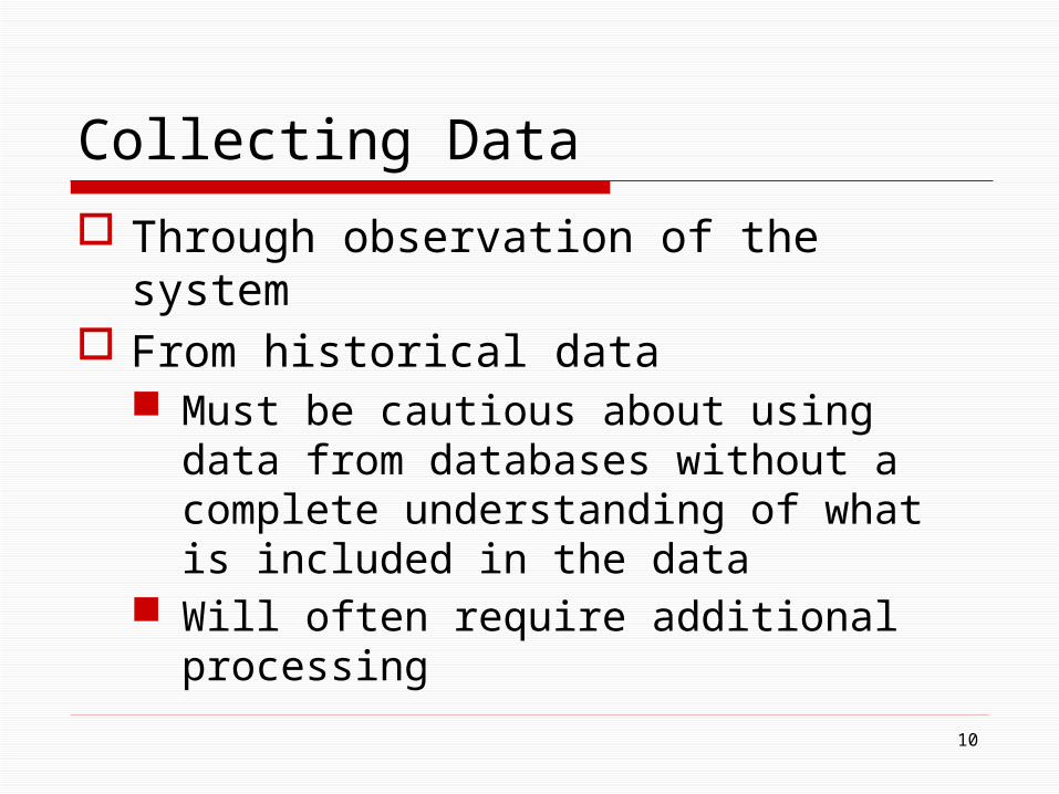
Through observation of the system From historical data

Must be cautious about using data from databases without a complete understanding of what is included in the data

Will often require additional processing

10

Collecting Data Through Observation - Example Simulation of vehicle traffic at an intersection.

Arrivals of cars to the intersection – what will you collect?

11

Collecting Data Through Observation - Planning

Create your data collection scenario Consider

What data will be recorded

Once data is collected

12

Input Analysis Assume you have “raw” data collected for

some random component of the system. Example: Service time data (minutes)

13

Obs # Day 1 Day 2 Day 3 Day 4 Day 5 Day 6 Day 71 3.5 0.4 5.1 1.1 0.8 1.2 1.02 5.2 0.6 3.2 1.2 3.6 3.3 4.13 0.7 2.0 0.7 3.3 1.2 0.4 0.74 8.9 1.7 1.5 0.2 4.7 4.0 1.25 0.8 1.3 0.2 3.8 1.1 0.8 0.16 2.6 1.0 3.0 1.8 1.0 0.9 1.87 0.9 0.1 4.6 4.7 0.7 1.3 0.48 1.3 4.4 5.2 5.7 0.9 10.6 0.09 1.4 1.2 5.1 0.4 4.8 1.9 1.710 1.9 0.9 0.2 4.7 6.4 0.8 0.7

Input Analysis The random component of the system will be

represented in the simulation model as observations from a probability distribution.

14

Input Analysis This process is called “fitting a distribution”.

Fitting a distribution - Selecting and justifying the proper distribution to use in the simulation to represent the random system component.

In general there are two choices for the type of distribution fitted.

15

Input Analysis When to use empirical distributions.

16

Input Analysis Empirical distributions

Generates observations that match the percentage of different observations in the collected data.

Example – Discrete case

17

XXX X XX X X X XX X X X XX X X X X1 2 3 4 5

Input Analysis

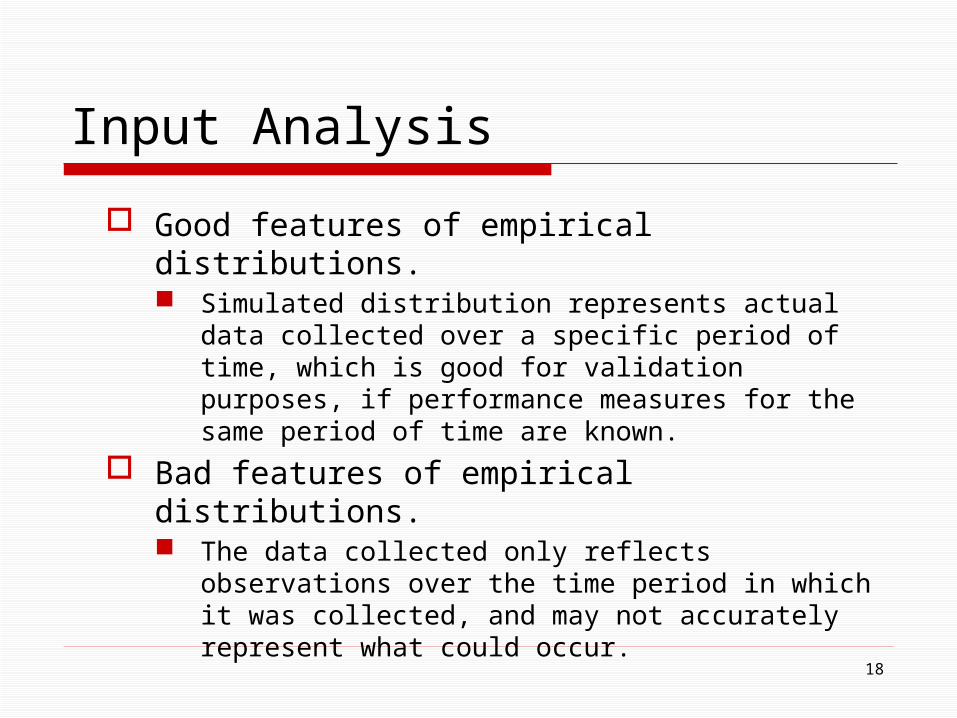
Good features of empirical distributions. Simulated distribution represents actual data

collected over a specific period of time, which is good for validation purposes, if performance measures for the same period of time are known.

Bad features of empirical distributions. The data collected only reflects observations over

the time period in which it was collected, and may not accurately represent what could occur.

18

Input Analysis

Arena Discrete empirical distribution

19

DISC(0.25, 1, 0.5, 1.25, 0.8, 1.75, 1.0, 2)

Input Analysis

Arena Continuous empirical distribution

20

CONT(0.25, 1, 0.5, 1.25, 0.8, 1.75, 1.0, 2)

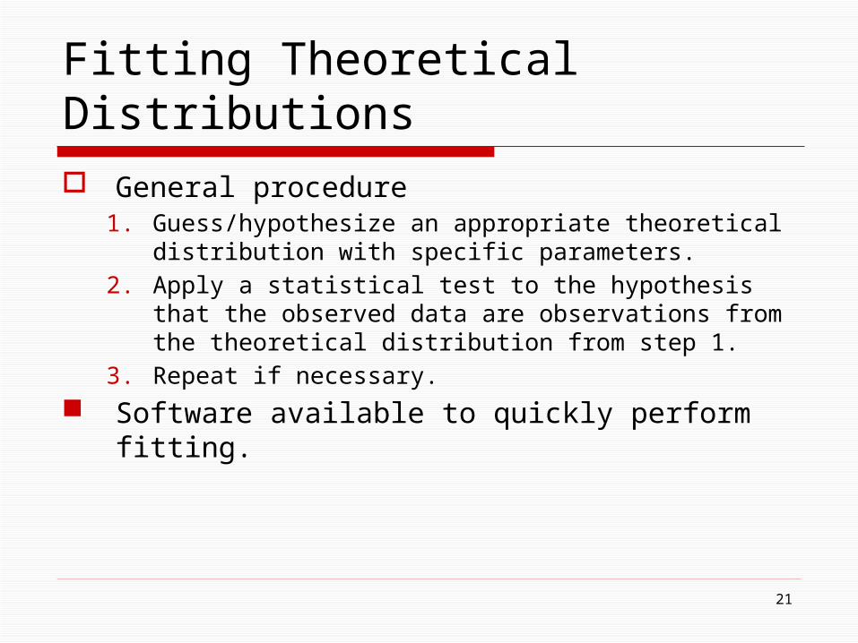
Fitting Theoretical Distributions General procedure

1. Guess/hypothesize an appropriate theoretical distribution with specific parameters.

2. Apply a statistical test to the hypothesis that the observed data are observations from the theoretical distribution from step 1.

3. Repeat if necessary. Software available to quickly perform fitting.

21

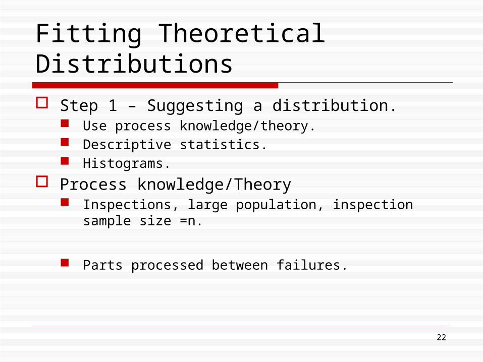
Fitting Theoretical Distributions Step 1 – Suggesting a distribution.

Use process knowledge/theory. Descriptive statistics. Histograms.

Process knowledge/Theory Inspections, large population, inspection sample size

=n.

Parts processed between failures.

22

Fitting Theoretical Distributions Process knowledge/Theory

Customer arrivals to a system from a large population.

Normal distribution.

23

Fitting Theoretical Distributions Descriptive statistics

Coefficient of variation (for X continuous) – CV(X) Different theoretical distributions have different values or

ranges of possible values. X~Exponential : CV= 1. X~U(a,b) :

X~Lognormal : 0 < CV < ∞.

)(3)(

ab

abXCV

24

Fitting Theoretical Distributions Descriptive statistics

Lexis ratio (for X discrete = Var(X)/E(X)) denoted τ(X) Different theoretical distributions have different values or

ranges of possible values. X~Geometric(p) : τ(X)= 1/p. X~Binomial(n,p) : τ(X)= 1-p. X~Poisson : τ(X)= 1.

25

Fitting Theoretical Distributions When data has been collected, the CV or lexis

ratio can be estimated from the data using the sample variance/standard deviation, and sample mean.

26

Fitting Theoretical Distributions Skewness – A measure of symmetry.

n

nsns

ns

nxx

XE

n

ii )1(*

)( where,)(

/)( skewness Sample

])[( Skewness

2

31

3

3

3

27

Fitting Theoretical Distributions Histograms – A graph of the frequency of

observations within predefined, non-overlapping intervals.

It is an estimate of the shape of a random variables probability mass function or density function.

Density functions/probability mass functions tend to have recognizable shapes.

28

Fitting Theoretical Distributions

29

Fitting Theoretical Distributions Making a histogram

1. Break up the range of values covered by the data into k disjoint intervals [b0,b1), [b1,b2),… ,[bk-1,bk). All intervals should be the same width Δb except for the first and last intervals (if necessary).

2. For j = 1,2,…,k, let qj = the proportion of the observations in the jth interval defined in 1.

3. Histogram value at x, h(x) = 0 if x < b0, qj if bj-1≤x<bj, and 0 if x ≥ bk.

30

Fitting Theoretical Distributions Making histograms

Histograms may be changed subjectively by changing the intervals and Δb (the interval size).

Guidelines (Hines, et al. 2003) Keep the number of intervals between 5 and 20. Set the number of intervals to be about the square

root of the number of observations.

31

In-class Exercise For data collected from

different random components of a system. Estimate the CV. Construct a histogram. Suggest a theoretical

distribution to represent the random component.

32

n Dist. 1 Dist. 2 Dist. 31 6.0 0.9 1.82 7.0 1.4 9.93 7.5 3.7 0.44 5.8 2.0 10.85 7.9 0.2 0.66 3.3 3.5 2.07 5.3 4.6 5.58 2.2 1.7 12.49 5.5 2.7 2.6

10 5.3 3.6 8.211 5.9 3.0 0.812 2.7 0.3 3.713 4.6 0.9 1.814 2.5 3.4 6.315 4.5 4.8 22.516 6.5 0.6 40.417 3.6 0.5 27.218 3.4 3.3 29.619 2.6 1.9 5.620 6.4 3.8 1.921 1.7 1.8 5.322 4.2 0.1 1.223 2.6 4.5 1.424 7.3 1.2 0.125 6.3 0.6 8.526 7.9 4.4 11.327 6.6 5.0 5.228 2.9 0.6 3.829 3.4 3.1 2.530 2.9 0.5 49.9

Sample Avg. 4.8 2.3 9.4StdDev. (est) 1.9 1.6 12.3

In-class Exercise

33

In-class Exercise

34

Parameter Estimation After suggesting a possible theoretical

distribution to represent a random system component, the parameters for that distribution must be estimated from the data (x1, x2, …, xn).

Different distributions may have a different number of parameters.

Estimating parameters from data for some distributions is intuitive.

35

Parameter Estimation Attention will be restricted to maximum likelihood

estimators or MLEs. Good statistical properties (needed as part of a

goodness of fit test). Examples of MLEs

X~Exponential(λ) λ = 1/E[X] The MLE for λ is

n

iix

n

1

36

Parameter Estimation Examples of MLEs

X~Uniform(a,b)

X~Normal(μ,σ2)

37

Parameter Estimation Not all MLEs for distribution parameters are so

intuitive. Example: X~Lognormal(σ,μ) where σ>0 is called a

shape parameter and μ Є (-∞, ∞) is called a scale parameter.

n

x

n

xn

ii

n

ii

1

2

1

)ˆ)(ln(ˆ ,

)ln(ˆ

38

Statistical Goodness of Fit Tests A distribution has been suggested to represent

a random component of a system. The data has been use to compute estimates

(MLE) of the distribution parameters. Statistical goodness of fit tests determine

whether there is enough evidence to say that the data is not well represented by the suggested distribution.

39

Statistical Goodness of Fit Tests Let be the suggested distribution with parameters

θ obtained from the data using MLE estimators. The statistical goodness of fit tests will evaluate the

null hypothesis

F

40

Statistical Goodness of Fit Tests

Three tests will be reviewed. Chi-square goodness of fit test. Kolmogorov-Smirnov test. Anderson-Darling test.

41

Chi-square Goodness of Fit Test Intuitively think of this test as a formal way to compare

a modified histogram to a theoretical distribution.

42

Chi-square Goodness of Fit Test Test procedure

1. Divide the entire range of the hypothesized distribution into k adjacent intervals – (a0,a1), [a1,a2),…,[ak-1,ak) where a0 could be -∞, and ak could be + ∞.

43


2. Tabulate the number of observations falling in each interval – (a0,a1), [a1,a2),…,[ak-1,ak). Let,

Nj = The number of observations falling in the jth interval [aj-1,aj).

∑ Nj = n :the total number of observations.

3. Calculate the expected number of observations in each interval from the suggested distribution and estimated parameters. Discrete Continuous

44

Chi-square Goodness of Fit Test Discrete

dist. for thefunction mass prob. )( where)(

ns.observatio ofnumber Total

where intervalin nsobservatio ofnumber Expected

1:

iaxai

ij

j

xpxpp

n

npj

jij

45

Chi-square Goodness of Fit Test Continuous

dist. for thefunction density prob. )( where)(

ns.observatio ofnumber Total

where intervalin nsobservatio ofnumber Expected

1

i

a

a

j

j

xfdxxfp

n

npj

j

j

46


4. Calculate the test statistic TS

. intervalin nsobservatio ofNumber where)(

1

2

jNnp

npNTS j

k

j j

jj

47

Chi-square Goodness of Fit Test If the distribution tested is a good fit, should TS

be large or small?

How do we know what large or small is? What do we compare TS to? What is the sampling distribution of the test statistic.

48

Chi-square Goodness of Fit Test Result – If MLE’s are used to estimate the m parameters

of a suggested distribution, then if H0 is true, as n→∞, the distribution of TS (the sampling distribution) converges to a Chi-square distribution that lies between two Chi-square distributions with k-1 and k-m-1 degrees of freedom.

If represents the value of the Chi-square distribution (df = degrees of freedom) such that of the area under the Chi-square distribution lies to the right of this value, then for the corresponding value for the distribution of TS

21, df

49

21,11

21,1 kmk TS

Chi-square Goodness of Fit Test

50

Density Function Plots for the Chi-Square Distribution

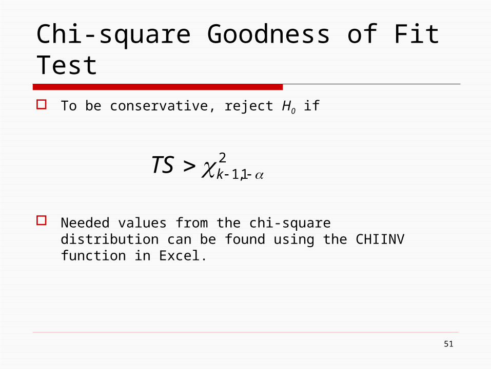
Chi-square Goodness of Fit Test To be conservative, reject H0 if

Needed values from the chi-square distribution can be found using the CHIINV function in Excel.

21,1 kTS

51

Chi-square Goodness of Fit Test As with histograms, there are no precise

answers for how to create intervals.

52

Example

53

Example

54

In-class Exercise

55

Chi-Square Goodness of Fit Test Exercise

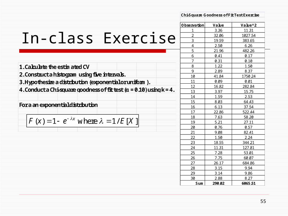
Observation Value Value^21 3.36 11.312 32.06 1027.543 19.59 383.654 2.50 6.265 21.96 482.266 0.41 0.177 0.31 0.108 1.22 1.509 2.89 8.3710 41.84 1750.2411 0.09 0.0112 16.82 282.8413 3.97 15.7514 1.59 2.5315 8.03 64.4316 6.13 37.5417 22.86 522.4418 7.63 58.2019 5.21 27.1120 0.76 0.5721 9.08 82.4122 1.50 2.2423 18.55 344.2124 11.31 127.8125 7.28 53.0126 7.75 60.0727 26.17 684.8628 3.15 9.9429 3.14 9.8630 2.88 8.27

Sum 290.02 6065.51

1. Calculate the estimated CV2. Construct a histogram using five intervals.3. Hypothesize a distribution (exponential or uniform).4. Conduct a Chi-square goodness of fit test (α = 0.10) using k = 4.

For a an exponential distribution

][/1where1)( XEexF x

In-class Exercise

56

In-class Exercise

57

Kolmogorov-Smirnov (K-S) Test

Pros Does not require partitioning of the data into

intervals. When the parameters of a distribution are known, it is

a more powerful test than the chi-square test (less probability of a type II error).

58


Cons Usually the parameters of a distribution are

estimated. Critical value (those values to compare to a test

statistic) have been estimated for some hypothesized distributions using Monte Carlo simulation. Normal Exponential Others (see Law and Kelton reference)

Difficult to use in the discrete case (ARENA Input Analyzer will generate no K-S test results).

59


The parameters known case is used when the distribution parameters are estimated, and estimated critical values are not available. This is conservative – The type I error is smaller than

specified.

60

Kolmogorov-Smirnov (K-S) Test The K-S test uses the empirical probability distribution

function generated from the data as a basis for computing a test statistic. Suppose there are n data observations collected, x1,…,xn.

The empirical distribution function Fn(x) is

This is a right continuous step function.

n

x'sxxF i

n

ofNumber )(

61

Example

62

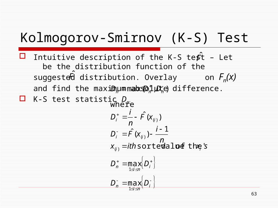
Kolmogorov-Smirnov (K-S) Test Intuitive description of the K-S test – Let be the

distribution function of the suggested distribution. Overlay on Fn(x) and find the maximum absolute difference.

K-S test statistic Dn:

F

F

63

ini

n

ini

n

ii

ii

ii

nnn

DD

DD

sxithxn

ixFD

xFn

iD

DDD

1

1

)(

)(

)(

max

max

' theof valuesorted

1)(ˆ

)(ˆwhere

),max(


64

Kolmogorov-Smirnov (K-S) Test Test – Reject if

1.4801.3581.2241.138c

.975.95.90.85

-1

where

11.012.0

-1

1

cDn

n n

65

F

66

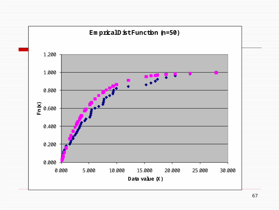
Kolomogorov-Smirnov Test - Example with 50 data points (not all shown)

(Expo(5)) Expo(mean=5)n Sample data Step Value F(x) Dn+ Dn- Test Statistic Critical value (alpha = 0.05)0 0.000 0.000 0.000 0.042 0.163 1.172 1.3581 0.119 0.020 0.024 -0.004 0.0242 0.157 0.040 0.031 0.009 0.0113 0.217 0.060 0.042 0.018 0.0024 0.311 0.080 0.060 0.020 0.0005 0.334 0.100 0.065 0.035 -0.0156 0.405 0.120 0.078 0.042 -0.0227 0.587 0.140 0.111 0.029 -0.0098 0.863 0.160 0.158 0.002 0.0189 0.895 0.180 0.164 0.016 0.00410 1.517 0.200 0.262 -0.062 0.08211 1.686 0.220 0.286 -0.066 0.08612 1.766 0.240 0.298 -0.058 0.07813 2.107 0.260 0.344 -0.084 0.10414 2.129 0.280 0.347 -0.067 0.08715 2.465 0.300 0.389 -0.089 0.10916 2.688 0.320 0.416 -0.096 0.11617 2.847 0.340 0.434 -0.094 0.11418 3.022 0.360 0.454 -0.094 0.11419 3.247 0.380 0.478 -0.098 0.11820 3.390 0.400 0.492 -0.092 0.11221 3.502 0.420 0.504 -0.084 0.10422 3.657 0.440 0.519 -0.079 0.09923 4.218 0.460 0.570 -0.110 0.13024 4.444 0.480 0.589 -0.109 0.12925 5.146 0.500 0.643 -0.143 0.16326 5.289 0.520 0.653 -0.133 0.15327 5.342 0.540 0.656 -0.116 0.13628 5.373 0.560 0.659 -0.099 0.11929 5.470 0.580 0.665 -0.085 0.10530 6.081 0.600 0.704 -0.104 0.124

67

0.000

0.200

0.400

0.600

0.800

1.000

1.200

0.000 5.000 10.000 15.000 20.000 25.000 30.000

Fn

(x)

Data value (X)

Emprical Dist Function (n=50)

In-class Exercise

68

n Data1 1.82 5.23 9.84 6.65 2.66 3.37 2.98 1.19 9.210 3.6

Conduct a K-S test to test the hypothesis that the data are observations from a U(0,10) distribution.

Anderson-Darling Test

Think of as a weighted K-S test. More weight given to differences

when the hypothesized probabilities are low – similar to percentage differences vs. absolute differences

69

Anderson-Darling Test

Critical values have been estimated for some hypothesized distributions

70

Goodness of Fit Tests

If a p-value is computed Low p-values (< 0.05) indicate a poor fit.

71

Assessing Independence It has been assumed that all observations of

data for some random system component are independent.

The chi-square, K-S, and A-D tests are testing for independent identically distributed random variables.

Most discrete event simulation models and software assume random components are independent.

72

Assessing Independence When presenting Monte Carlo simulation we

talked about correlation. Two or more random components of a simulation

(e.g., engineering economic calculation) may be correlated. E.g., Repair costs in year one and year two. There was no simulated time component in these

simulations. In discrete event simulation correlation may

occur, Between different random components. Within the same random component.

73

Assessing Independence Examples

Different random components.

Within the same random component.

74

Recognizing Non-independence Method 1 – Correlation estimates and

hypothesis testing. E.g., Rank correlation estimates.

Method 2 – Correlation plot. Method 3 – Scatter diagram.

75

Recognizing Non-independence Let x1, x2,…, xn be collected data listed in the time

order of collection. Sample correlation

As j approaches n this estimate is very poor since the number of values used for the estimate is small.

jn

xxxxC

C

jn

ijii

j

jj

1

2

))((ˆ

ˆ

ˆˆ

76

Recognizing Non-independence Scatter plot.

Plot of (xi, xi+1) or (xi,yi).

Visual subjective interpretation.

77

Recognizing Non-independence Correlation plot – Applicable when examining

correlation within a single random component. Plot Cj vs. j.

78

Example Wait in queue. Correlated?

Single server system – Utilization = 0.98

79

0 20 40 60 80 100 120 1400.00

5.00

10.00

15.00

20.00

25.00

30.00

Wait in Q vs. Time

Simulation Time (minutes)

Q T

ime (

Min

ute

s)

Example – Correlation Estimates

80

Queue Times from an M/M/1 system - Util = .98 Correlation EstimatesLag 1 Lag 2

Average Variance 0.79 0.589.23 69.47

Customer Time (minutes) Queue Time (min) (xi-xbar)(xi+1-xbar) (xi-xbar)(xi+2-xbar)1 0 0.00 82.43 85.272 1.48 0.31 82.43 82.433 2.10 0.00 85.27 85.274 2.57 0.00 85.27 85.275 12.28 0.00 85.27 36.866 18.81 0.00 36.86 85.277 24.53 5.24 36.86 35.188 29.84 0.00 81.40 85.279 32.40 0.42 81.40 -19.9510 33.18 0.00 -20.90 -139.0011 45.36 11.50 34.07 17.3412 65.15 24.29 115.35 34.1813 65.21 16.90 17.40 19.9014 66.07 11.51 5.90 3.4915 71.03 11.83 4.00 13.8816 74.61 10.77 8.23 5.7217 79.38 14.58 19.86 75.8418 79.85 12.95 52.72 37.5919 92.13 23.42 143.55 153.2520 92.42 19.35 109.28 113.4821 93.71 20.04 121.16 75.8722 100.67 20.45 78.79 66.4523 101.88 16.26 41.61 41.1024 104.54 15.16 34.66 32.7725 106.49 15.09 32.37 -4.1826 107.59 14.77 -3.95 -30.6927 111.80 8.52 3.96 6.5928 114.83 3.69 51.22 51.2229 120.73 0.00 85.2730 123.18 0.00

Example – Scatter Diagram

81

0.00 5.00 10.00 15.00 20.00 25.00 30.000.00

5.00

10.00

15.00

20.00

25.00

30.00

xi vs. xi+1

xi

xi+

1

Example Scatter Diagram – Zero Correlation

82

0

5

10

15

20

25

30

0 5 10 15 20 25 30

X(i

+1)

X(i)

Scatter Diagram

Series1

Recognizing Non-independence If you determine that correlations exist, what

do you do?

84

What to do with Minimal Information? Suppose you cannot collect data or that none is

available. Suggested no data distributions.

85

Possible No-Data DistributionsDistribution Characteristics ExamplesExponential CV = 1 Interarrival Times

Non-negative (minimum = 0) Time between failuresNo maximum valueNon symmetric

Triangular Symmetric or non-symmetric Activity timesFinite rangeEasily interpreted parameters(Min, Max, Mode)

Uniform Finite range Little known about processAll values equally likely

What to do with Minimal Information?

Getting information about distribution parameters.

86

Non-stationary Arrival Processes A very common feature of many systems (in particular

service systems) is that the arrival rate (e.g., customers) varies as a function of time. The arrival process is called non-stationary.

87

Non-stationary Arrival Processes

A practical method to approximate a non-stationary arrival process is to use a “piecewise constant” rate function.

Over predefined time intervals assume a constant (and different) arrival rate.

88


Example – A very common arrival process used in simulation is the Poisson process.

89


Implementation of a non-stationary Poisson process. Common but incorrect approach.

Have the mean interarrival time (or interarrival rates) be represented with a variable. Change the value of this variable for each interval.

90


What’s wrong with this approach?

91

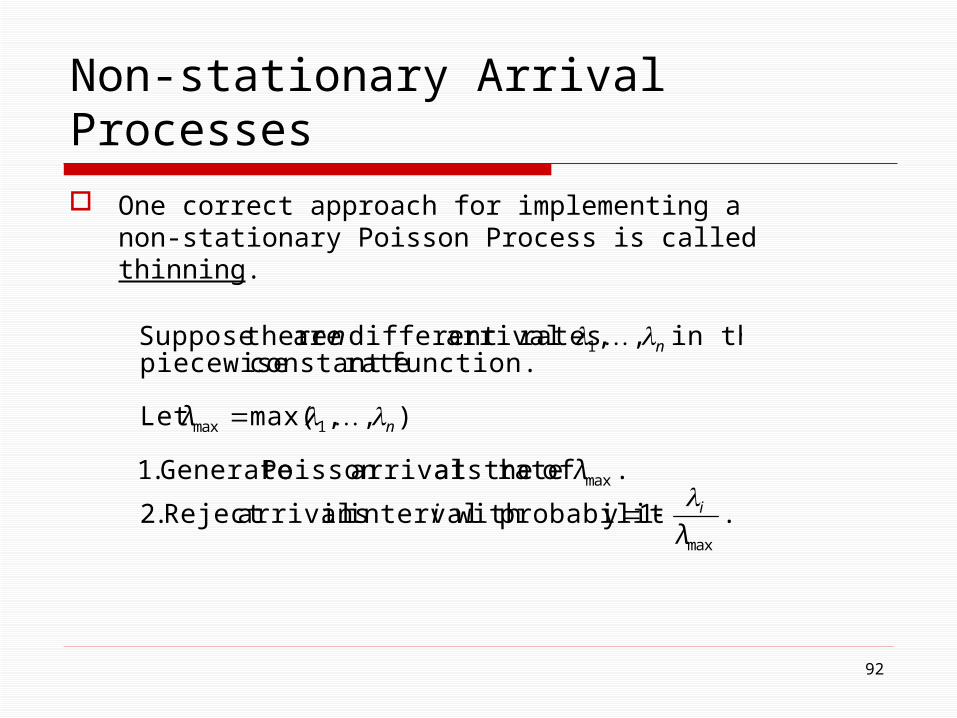
Non-stationary Arrival Processes One correct approach for implementing a non-

stationary Poisson Process is called thinning.

.1 y probabilit with intervalin arrivalsReject .2

. of rate at the arrivalsPoisson Generate .1

),,max(Let

function. rateconstant piecewise in the ,, rates arrivaldifferent are thereSuppose

max

max

1max

1

λi

λ

λ

n

i

n

n

92


93

Non-stationary Arrival Processes Arena

implements a correct non-stationary Poisson arrival process.

94


95

Input Analysis 1. Initial steps of the simulation study have been completed. Through a verbal...

Documents

Transcript of Input Analysis 1. Initial steps of the simulation study have been completed. Through a verbal...