![[2009] [05] Innovative Ship Designocw.snu.ac.kr/sites/default/files/NOTE/5520.pdf* 선박설계는무에서유를창조하는혁신적인업무라기보다는 실적자료를토대로한개선](https://static.fdocuments.in/doc/165x107/5e5c3b2f2c2fa7353d5db532/2009-05-innovative-ship-eeeeoeoeeeeeeeee.jpg)
Innovative ship design -Integral Equation and...
76
Innovative Ship Design - Elasticity SDAL @ Advanced Ship Design Automation Lab. http://asdal.snu.ac.kr Seoul National Univ. Naval Architecture & Ocean Engineering SDAL @ Advanced Ship Design Automation Lab. http://asdal.snu.ac.kr Seoul National Univ. July 2009 Prof. Kyu-Yeul Lee Department of Naval Architecture and Ocean Engineering, Seoul National University of College of Engineering [2009] [15] Innovative ship design - Integral Equation and Approximation-
Transcript of Innovative ship design -Integral Equation and...

Innovative Ship Design - ElasticitySDAL@Advanced Ship Design Automation Lab.http://asdal.snu.ac.kr
Seoul NationalUniv.
Naval A
rch
itect
ure
& O
cean
En
gin
eeri
ng
SDAL@Advanced Ship Design Automation Lab.http://asdal.snu.ac.kr
Seoul NationalUniv.
July 2009Prof. Kyu-Yeul Lee
Department of Naval Architecture and Ocean Engineering,Seoul National University of College of Engineering
[2009] [15]
Innovative ship design
- Integral Equation and Approximation-

Innovative Ship Design - ElasticitySDAL@Advanced Ship Design Automation Lab.http://asdal.snu.ac.kr
Seoul NationalUniv.
weak form : ‘weighted average’*
Contents
Approximation
Governing Equation
Differential Approach Energy Method
Stress
Strain
Displacement
Force Equilibrium
Generalized Hooke’ Law
Compatibility
Analytic Solution
Elasticity
Strain Energy, 0m= =∑F a a in equilibrium
Virtual Displacement
Virtual Work
FEM
Rayleigh-Ritz MethodGalerkin Method
Deflection Curve of the BeamScantling
2
Wang,C.T., Applied Elasticity , McGRAW-HILL, 1953응용탄성학, 이원 역, 숭실대학교 출판부, 1998
Chou,P.C.,Elasticity (Tensor, Dyadic, and Engineering Approached), D. Van
Nostrand, 1967
Gere,J.M.,Mechanics of Materials, Sixth Edition, Thomson, 2006
Hildebrand,F.B., ”Methods of Applied Mathematics”, 2nd edition, Dover, 1965
Becker,E.B., “Finite Elements, An Introduction”, Vol.1, Prentice-Hall, 1981
Fletcher,C.A.J., “Computational Galerkin Methods”, Springer, 1984
1 2
1
Becker,E.B., “Finite Elements, An Introduction”, Vol.1, Prentice-Hall, 1981, chapter1
Innovative Ship Design - ElasticitySDAL@Advanced Ship Design Automation Lab.http://asdal.snu.ac.kr
Seoul NationalUniv.
Summary
2( ) 0eG G u Xx
λ ∂+ + ∇ + =
∂2( ) 0eG G v Y
yλ ∂+ + ∇ + =
∂
2( ) 0eG G w Zz
λ ∂+ + ∇ + =
∂
(1 )(1 2 ) (1 )
(1 )(1 2 ) (1 )
(1 )(1 2 ) (1 )
x x
y y
z z
E Ee
E Ee
E Ee
νσ εν ν ννσ εν ν ννσ εν ν ν
= ++ − +
= ++ − +
= ++ − +
, x y ze ε ε ε= + +
,2( 1)
,2( 1)
,2( 1)
xy xy
yz yz
zx zx
E
E
E
τ γν
τ γν
τ γν
=+
=+
=+
6 Relations btw. 6 Strain and 6 Stress
6 Relations btw. Strain and Displacement
, , ,
, ,
x y z
xy yz zx
u v wx y zu v v w w uy x z y x z
ε ε ε
γ γ γ
∂ ∂ ∂= = =∂ ∂ ∂∂ ∂ ∂ ∂ ∂ ∂
= + = + = +∂ ∂ ∂ ∂ ∂ ∂
6 Equations of force equilibrium
0
0
0
yxx zxx
xy y zyy
yzxz zz
F Xx y z
F Yx y z
F Zx y z
τσ τ
τ σ τ
ττ σ
∂∂ ∂= + + + =
∂ ∂ ∂∂ ∂ ∂
= + + + =∂ ∂ ∂
∂∂ ∂= + + + =
∂ ∂ ∂
∑
∑
∑
0
0
0
x yz zy
y xz zx
z xy yx
M
M
M
τ τ
τ τ
τ τ
= − =
= − =
= − =
∑∑∑
, , , , , , , ,x yx zx xy y zy xz yz zσ τ τ τ σ τ τ τ σ
, ,u v w, , , , ,x y z xy yz zxε ε ε γ γ γ6 Strain
9 Stress
3 Displacement
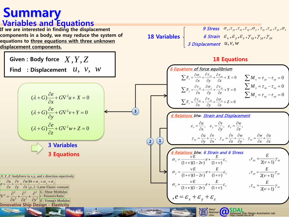
18 Variables
, ,u v wGiven : Body force , ,X Y ZFind : Displacement
12
3
18 Equations
3 Variables
3 Equations
If we are interested in finding the displacement components in a body, we may reduce the system of equations to three equations with three unknown displacement components.
Variables and Equations
, : Lame Elastic constantµ λ:Shear MoldulusG
: Young's ModulusE
u v wex y z∂ ∂ ∂
= + +∂ ∂ ∂
, , : bodyforce in x,y, and z direction repectivelyX Y Z
: Poisson's Ratioν2 2 2
22 2 2x z y
∂ ∂ ∂∇ = + +
∂ ∂ ∂
x y zσ σ σΘ = + +

Innovative Ship Design - ElasticitySDAL@Advanced Ship Design Automation Lab.http://asdal.snu.ac.kr
Seoul NationalUniv.
Summary
Given : Body force
(1 )(1 2 ) (1 )
(1 )(1 2 ) (1 )
(1 )(1 2 ) (1 )
x x
y y
z z
E Ee
E Ee
E Ee
νσ εν ν ννσ εν ν ννσ εν ν ν
= ++ − +
= ++ − +
= ++ − +
, x y ze ε ε ε= + +
,2( 1)
,2( 1)
,2( 1)
xy xy
yz yz
zx zx
E
E
E
τ γν
τ γν
τ γν
=+
=+
=+
6 Relations btw. 6 Strain and 6 Stress
6 Equations of force equilibrium
0
0
0
yxx zxx
xy y zyy
yzxz zz
F Xx y z
F Yx y z
F Zx y z
τσ τ
τ σ τ
ττ σ
∂∂ ∂= + + + =
∂ ∂ ∂∂ ∂ ∂
= + + + =∂ ∂ ∂
∂∂ ∂= + + + =
∂ ∂ ∂
∑
∑
∑
0
0
0
x yz zy
y xz zx
z xy yx
M
M
M
τ τ
τ τ
τ τ
= − =
= − =
= − =
∑∑∑, ,X Y Z
2
1
3
15 Equations
22
22
22
1 01
1 01
1 01
xy
yz
zx
Y Xx y x y
Z Yy z y z
X Zz x z x
τν
τν
τν
∂ ∂ ∂ Θ+ +∇ + = ∂ ∂ + ∂ ∂
∂ ∂ ∂ Θ+ +∇ + = ∂ ∂ + ∂ ∂
∂ ∂ ∂ Θ + +∇ + = ∂ ∂ + ∂ ∂
22
2
22
2
22
2
12 01 1
12 01 1
12 01 1
x
y
z
X Y Z Xx y z x x
X Y Z Yx y z y y
X Y Z Zx y z z z
ν σν ν
ν σν ν
ν σν ν
∂ ∂ ∂ ∂ ∂ Θ+ + + +∇ + = − ∂ ∂ ∂ ∂ + ∂
∂ ∂ ∂ ∂ ∂ Θ+ + + +∇ + = − ∂ ∂ ∂ ∂ + ∂
∂ ∂ ∂ ∂ ∂ Θ+ + + +∇ + = − ∂ ∂ ∂ ∂ + ∂
, , , , ,x y z xy yz zxσ σ σ τ τ τFind : Stress
6 Variables6 Equations
, , , , , , , ,x yx zx xy y zy xz yz zσ τ τ τ σ τ τ τ σ
, ,u v w, , , , ,x y z xy yz zxε ε ε γ γ γ6 Strain
9 Stress
3 Displacement
15 Variables
6 Relations btw. Strain and Displacement
, , ,
, ,
x y z
xy yz zx
u v wx y zu v v w w uy x z y x z
ε ε ε
γ γ γ
∂ ∂ ∂= = =∂ ∂ ∂∂ ∂ ∂ ∂ ∂ ∂
= + = + = +∂ ∂ ∂ ∂ ∂ ∂
2
2
2
2
2
2
yz xyx zx
y yz xyzx
yz xyzxz
y z x x y z
orz x y x y z
x y z x y z
γ γε γ
ε γ γγ
γ γγε
∂ ∂ ∂ ∂∂= − + + ∂ ∂ ∂ ∂ ∂ ∂
∂ ∂ ∂ ∂∂ = − + ∂ ∂ ∂ ∂ ∂ ∂ ∂ ∂ ∂∂ ∂ = + − ∂ ∂ ∂ ∂ ∂ ∂
2 22
2 2
2 22
2 2
2 22
2 2
y xyx
y yzz
x zxz
y x x y
z y y z
x z z x
ε γε
ε γε
ε γε
∂ ∂∂+ =
∂ ∂ ∂ ∂∂ ∂∂ + = ∂ ∂ ∂ ∂ ∂ ∂∂
+ =∂ ∂ ∂ ∂
Compatibility equations 3 independent Equations
18 Variables
18 EquationsIf we are interested in finding only the stress components in a body, we may reduce the system of equations to six equations with six unknown stress components
, : Lame Elastic constantµ λ:Shear MoldulusG
: Young's ModulusE
u v wex y z∂ ∂ ∂
= + +∂ ∂ ∂
, , : bodyforce in x,y, and z direction repectivelyX Y Z
: Poisson's Ratioν2 2 2
22 2 2x z y
∂ ∂ ∂∇ = + +
∂ ∂ ∂
x y zσ σ σΘ = + +

Innovative Ship Design - ElasticitySDAL@Advanced Ship Design Automation Lab.http://asdal.snu.ac.kr
Seoul NationalUniv.
Differential Equation (ODE/PDE)
Classification
Integral Equations
Variational formulation
Rayleigh-Ritz Approximate Method
Galerkin
Collocation
Least Square
Approximate Method
Volterra
Weak Form2)Approximate Method4)
Galerkin
Collocation
Least Square
FEM
( ) ( ) ( ) ( , ) ( )x
ax y x F x K x y dα λ ξ ξ ξ= + ∫
( ) ( ) ( ) ( , ) ( )b
ax y x F x K x y dα λ ξ ξ ξ= + ∫
Fredholm
Leibnitz formula1)
( ) ( )
( ) ( )
( , )( , ) [ , ( )] [ , ( )]B x B x
A x A x
d d F x dB dAF x d d F x B x F x A xdx dx x dx dx
ξξ ξ ξ∂= + −
∂∫ ∫
1) Jerry, A.j., Introduction to Integral Equations with Applications, Marcel Dekker Inc., 1985, p19~252) ‘variational statement of the problem’ -Becker, E.B., et al, Finite Elements An Introduction, Volume 1, Prentice-Hall, 1981, p43) Becker, E.B., et al, Finite Elements An Introduction, Volume 1, Prentice-Hall, 1981, p2 . See also Betounes, Partial Differential Equations for Computational Science, Springer, 1988, p408 “…the weak solution is actually a strong (or classical) solution…”4) some books refer as ‘Method of Weighted Residue’ from the Finite Element Equation point of view and they have different type depending on how to choose the weight functions. See also Fletcher,C.A.J., “Computational Galerkin Methods”, Springer, 19845) Jerry, A.j., Introduction to Integral Equations with Applications, Marcel Dekker Inc., 1985, p1 “Problems of a ‘hereditary’ nature fall under the first category, since the state of the system u(t) at any time t depends by the definition on all the previous states u(t-τ) at the previous time t-τ ,which means that we must sum over them, hence involve them under the integral sign in an integral equation.
whenever a smooth ‘classical(strong)’ solution to a (D.E.) problem exists, it is also the solution of the weak problem3) 1
0( ) 0
(0 )0, (1) 0
u u x v dx
u u
′′− + − =
= =∫ 1
0( ) 0u v uv xv dx′ ′− + − =∫
integration by part and demand the test functions vanish at the endpoints
2 0d dyT y pdx dx
ρω + + =
Ex.)2
2 2
0
1 02 2
l T dyy py dxdx
δ ρω + − =
∫
, 0 1,(0 )0, (1) 0u u x x
u u′′− + = < <= =
Ex.) Work and Energy Principle
1( ) ( )
n
k k i ik
c s x F x=
=∑
( ) ( )2
1min
nb
k kak
c s x F x dx=
− ∑∫
1( ) ( ) ( ) ( )
n b b
k i k ia ak
c x s x dx x F x dxψ ψ=
=∑ ∫ ∫
1, ( ) ( )n
k ikx a xψ φ
==∑
1( ) ( )
n
k kk
c s x F x=
≈∑ , ( ) ( ) ( , ) ( )b
k k as x x K x y dφ λ ξ ξ ξ= − ∫
assume:
0 1 1( ) ( ) ( ) ( )n ny x x c x c xφ φ φ≈ + + +
problem of a “hereditary’ nature5)
multiply and integration yδ
integration by part and B/C
2
0
l d dyT y p y dxdx dx
ρω δ + + ∫
multiply and integration v1
( ) ( )nj jj
u x c xφ=
≈ ∑1
( ) ( )ni ii
v x a xφ=
≈ ∑
- Variation and integration- Integration and variation
( ) ( ) ( ) ( ){ } ( )1 1
0 01 1 1
N N N
i i i j i j i ii j i
a c x x x x dx a x x dxφ φ φ φ φ= = =
′ ′ + = ∑ ∑ ∑∫ ∫
1
nj ij ii
c k F=
=∑
ijkiF
1 2 3 4x( )1 xφ
( )2 xφ
( )3 xφ
shape function
what is the relationship between ‘week form’ and ‘Variational formulation’?
[ ]1 11
00 0( ) ( )u v dx u v u v dx′′ ′ ′ ′− = − +∫ ∫
Innovative Ship Design - ElasticitySDAL@Advanced Ship Design Automation Lab.http://asdal.snu.ac.kr
Seoul NationalUniv.
Summary : Integral Equations

Innovative Ship Design - ElasticitySDAL@Advanced Ship Design Automation Lab.http://asdal.snu.ac.kr
Seoul NationalUniv.
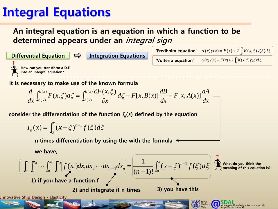
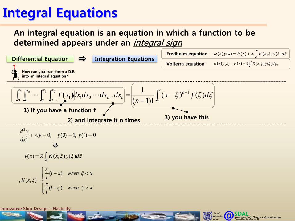
Integral EquationsAn integral equation is an equation in which a function to be determined appears under an integral sign
( ) ( ) ( ) ( , ) ( )b
ax y x F x K x y dα λ ξ ξ ξ= + ∫‘Fredholm equation’
, F and Kαwhere are given function and , ,a bλ are constant
The function is to be determined( )y x
( ) ( ) ( ) ( , ) ( ) ,x
ax y x F x K x y dα λ ξ ξ ξ= + ∫‘Volterra equation’
upper limit of integral is not a constant
The given function , which depends upon the current variable x as well as the auxiliary variable ξ, is known as the kernel of the integral equation
( , )K x ξ
Can you guess what decides the type of integral equation?
What is the relationship between D.E. and the integral equations?
Differential Equation Integral Equations
How can you transform a D.E. into an integral equation?

Innovative Ship Design - ElasticitySDAL@Advanced Ship Design Automation Lab.http://asdal.snu.ac.kr
Seoul NationalUniv.
Integral EquationsAn integral equation is an equation in which a function to be determined appears under an integral sign
Differential Equation Integration Equations
How can you transform a D.E. into an integral equation?
( ) ( ) ( ) ( , ) ( )b
ax y x F x K x y dα λ ξ ξ ξ= + ∫‘Fredholm equation’
( ) ( ) ( ) ( , ) ( ) ,x
ax y x F x K x y dα λ ξ ξ ξ= + ∫‘Volterra equation’
it is necessary to make use of the known formula( ) ( )
( ) ( )
( , )( , ) [ , ( )] [ , ( )]B x B x
A x A x
d F x dB dAF x d d F x B x F x A xdx x dx dx
ξξ ξ ξ∂= + −
∂∫ ∫
1( ) ( ) ( )x n
n aI x x f dξ ξ ξ−= −∫
consider the differentiation of the function In(x) defined by the equation
n times differentiation by using the with the formula
3 2 11 1 2 1
1( ) ( ) ( )( 1)!
nx x x x x nn na a a a a
f x dx dx dx dx x f dn
ξ ξ ξ−− = −
−∫ ∫ ∫ ∫ ∫
we have,
What do you think the meaning of this equation is?
1) if you have a function f
2) and integrate it n times 3) you have this
Innovative Ship Design - ElasticitySDAL@Advanced Ship Design Automation Lab.http://asdal.snu.ac.kr
Seoul NationalUniv.
Integral EquationsAn integral equation is an equation in which a function to be determined appears under an integral sign
Differential Equation Integration Equations
How can you transform a D.E. into an integral equation?
( ) ( ) ( ) ( , ) ( )b
ax y x F x K x y dα λ ξ ξ ξ= + ∫‘Fredholm equation’
( ) ( ) ( ) ( , ) ( ) ,x
ax y x F x K x y dα λ ξ ξ ξ= + ∫‘Volterra equation’
3 2 11 1 2 1
1( ) ( ) ( )( 1)!
nx x x x x nn na a a a a
f x dx dx dx dx x f dn
ξ ξ ξ−− = −
−∫ ∫ ∫ ∫ ∫
1) if you have a function f
2) and integrate it n times 3) you have this
2
2 0, (0) 1, ( ) 0d y y y y ldx
λ+ = = =
0( ) ( , ) ( )
ly x K x y dλ ξ ξ ξ= ∫
( ), ( , )
( )
l x when xlK xx l when xl
ξ ξξ
ξ ξ
− <= − >

Innovative Ship Design - ElasticitySDAL@Advanced Ship Design Automation Lab.http://asdal.snu.ac.kr
Seoul NationalUniv.
Differential Equation and Integral Equations
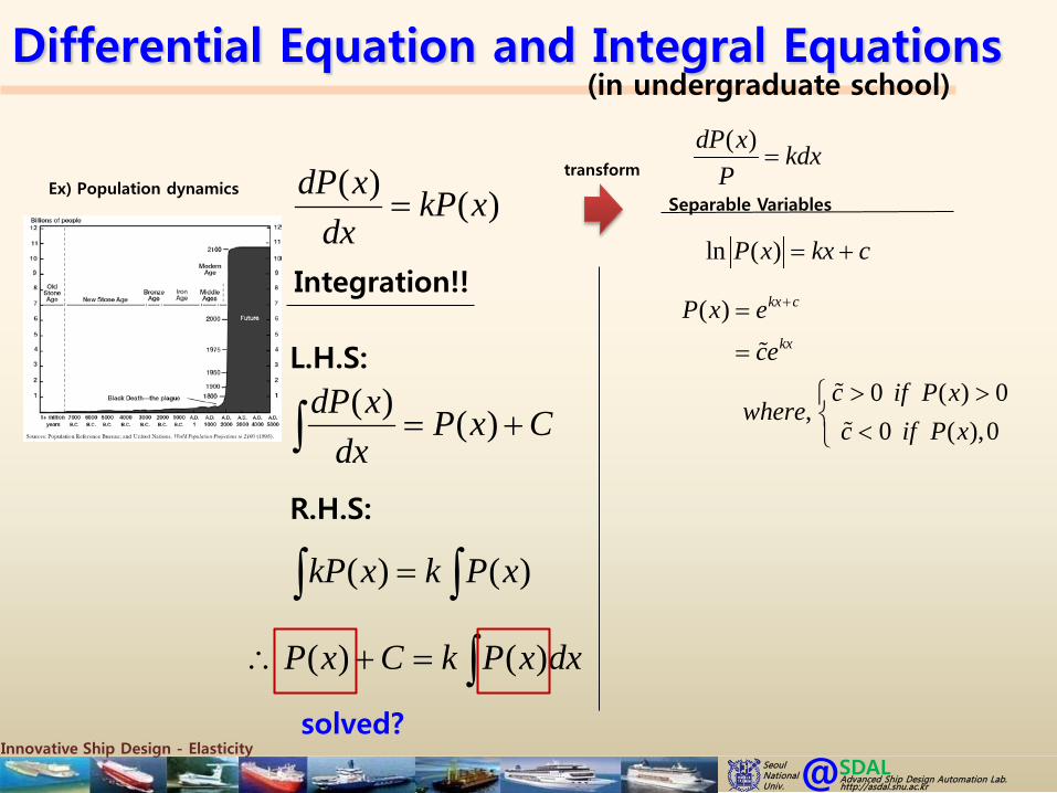
Ex) Population dynamics
( ) ( )dP t kP tdt
=Integration!!
( ) ( )dP t dx P t Cdt
= +∫
L.H.S:
( ) ( )kP t dt k P t dt=∫ ∫R.H.S:
( ) ( )P t C k P t d x∴ + = ∫solved?
How to solve a Differential Equation?
Integration!
Then, how?
(in undergraduate school)
Innovative Ship Design - ElasticitySDAL@Advanced Ship Design Automation Lab.http://asdal.snu.ac.kr
Seoul NationalUniv.
Differential Equation and Integral Equations
Ex) Population dynamics )()( xkPdx
xdP=
Integration!!
CxPdx
xdP+=∫ )()(
L.H.S:
∫∫ = )()( xPkxkP
R.H.S:
∫=+∴ dxxPkCxP )()(
solved?
Separable Variables
kdxP
xdP=
)(
ln ( )P x kx c= +
transform
(in undergraduate school)
( )
0 ( ) 0,
0 ( ),0
kx c
kx
P x ece
c if P xwhere
c if P x
+=
=
> > <

Innovative Ship Design - ElasticitySDAL@Advanced Ship Design Automation Lab.http://asdal.snu.ac.kr
Seoul NationalUniv.
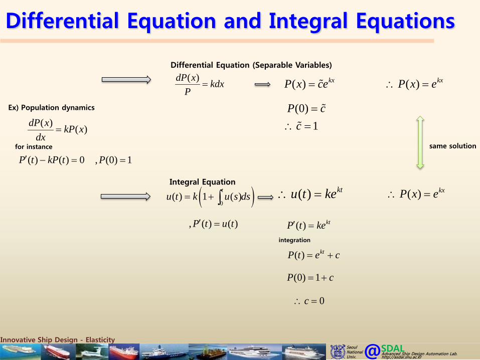
Differential Equation and Integral Equations
Ex) Population dynamics
( ) ( )dP t kP tdt
=
How to solve a Differential Equation?
Integration!
(in graduate school)
for instance
, (0) 1P =( ) ( ) 0P t kP t′ − =
( ) ( )let P t u t′ =
0( ) (0) ( )
tP t P u s ds− = ∫
0( ) 1 ( )
tP t u s ds∴ = + ∫
( ) ( ) 0P t kP t′ − =
( )0( ) 1 ( ) 0
tu t k u s ds− + =∫
( )0( ) 1 ( ) (1)
tu t k u s ds= + ∫
Integral Equation Then, how to solve?
By using decomposition methods*
* Wazwaz, A.M., A First Course in Integral Equations, World Scientific, 1997, ch3.2
0( ) ( ) (2 )nn
u t u t∞
== ∑
0 0( ) ( )
t tP s ds u s ds′ =∫ ∫
integration both sides
Substituting (2) into (1)
( )( )0 1 2 0 1 20( ) ( ) ( ) 1 ( ) ( ) ( )
tu t u t u t k u s u s u s d s+ + + = + + + +∫
0
1 00
2 10
( )
( ) ( )
( ) ( )
t
t
u t k
u t k u s ds
u t k u s ds
=
=
=
∫∫
[ ]2 21 00( )
t tu t k kds k s k t= = =∫3 3
2 2 22 00( )
2 2t tk ku t k k s ds s t = = = ∫
2 31 1( ) ( ) ( )2 2 3
u t k k kt k kt k kt= + ⋅ + + +⋅
2 31 11 ( ) ( )2 2 3
k kt kt kt = + + + + ⋅
( ) ktu t ke∴ =
Innovative Ship Design - ElasticitySDAL@Advanced Ship Design Automation Lab.http://asdal.snu.ac.kr
Seoul NationalUniv.
Differential Equation and Integral Equations
Ex) Population dynamics
)()( xkPdx
xdP=
for instance
, (0) 1P =( ) ( ) 0P t kP t′ − =
kdxP
xdP=
)(Differential Equation (Separable Variables)
( )0( ) 1 ( )
tu t k u s ds= + ∫Integral Equation
, ( ) ( )P t u t′ =
( ) kxP x ce=
(0)1
P cc
=∴ =
( ) kxP x e∴ =
( ) ktu t ke∴ =
( ) ktP t ke′ =
(0) 1P c= +
( ) ktP t e c= +
integration
0c∴ =
( ) kxP x e∴ =
same solution
Innovative Ship Design - ElasticitySDAL@Advanced Ship Design Automation Lab.http://asdal.snu.ac.kr
Seoul NationalUniv.
Differential Equation and Integral Equations
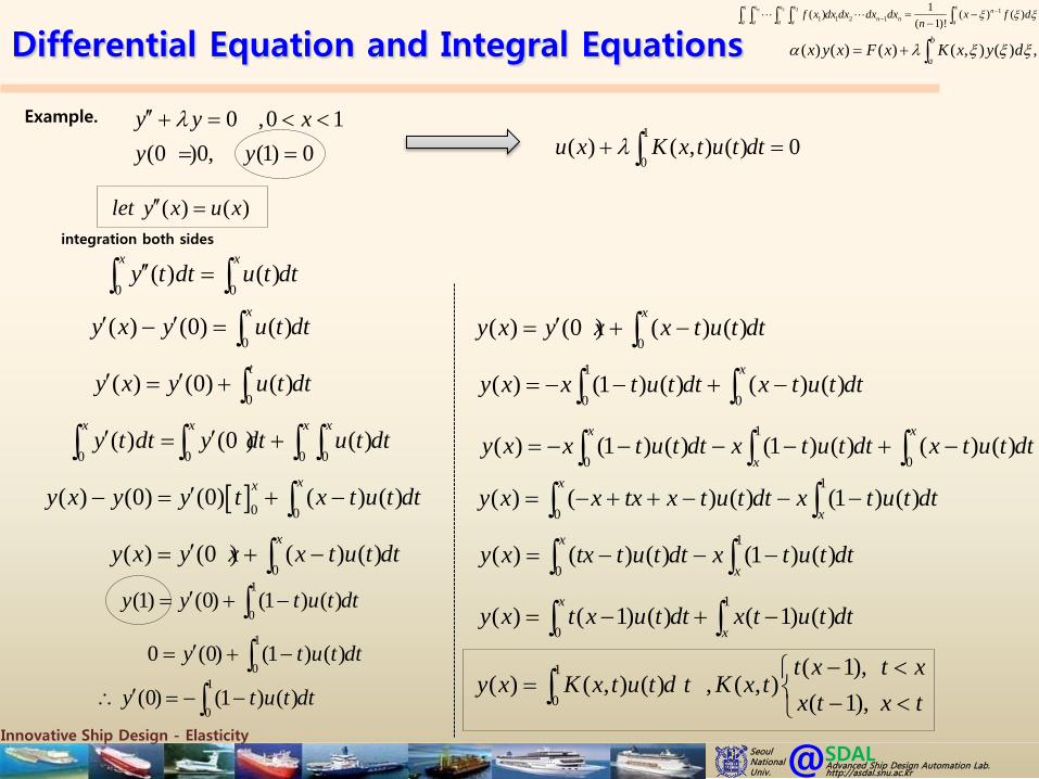
Example. 0 ,0 1(0 )0, (1) 0
y y xy y
λ′′ + = < <= =
( ) ( )let y x u x′′ =
0( ) (0) ( )
xy x y u t dt′ ′− = ∫
0( ) (0) ( )
ty x y u t dt′ ′= + ∫
0 0( ) ( )
x xy t dt u t dt′′ =∫ ∫
integration both sides
0 0 0 0( ) (0 ) ( )
x x x xy t dt y dt u t dt′ ′= +∫ ∫ ∫ ∫
[ ]0 0( ) (0) (0) ( ) ( )
xxy x y y t x t u t dt′− = + −∫
0( ) (0 ) ( ) ( )
xy x y x x t u t dt′= + −∫
1
0(1) (0) (1 ) ( )y y t u t dt′= + −∫
1
00 (0) (1 ) ( )y t u t dt′= + −∫
1
0(0) (1 ) ( )y t u t dt′∴ = − −∫
0( ) (0 ) ( ) ( )
xy x y x x t u t dt′= + −∫
1
0 0( ) (1 ) ( ) ( ) ( )
xy x x t u t dt x t u t dt= − − + −∫ ∫
1
0 0( ) (1 ) ( ) (1 ) ( ) ( ) ( )
x x
xy x x t u t dt x t u t dt x t u t dt= − − − − + −∫ ∫ ∫
1
0( ) ( ) ( ) (1 ) ( )
x
xy x x tx x t u t dt x t u t dt= − + + − − −∫ ∫
1
0( ) ( ) ( ) (1 ) ( )
x
xy x tx t u t dt x t u t dt= − − −∫ ∫
1
0( ) ( 1) ( ) ( 1) ( )
x
xy x t x u t dt x t u t dt= − + −∫ ∫
1
0
( 1),( ) ( , ) ( ) , ( , )
( 1),t x t x
y x K x t u t d t K x tx t x t
− <= − <∫
1
0( ) ( , ) ( ) 0u x K x t u t dtλ+ =∫
3 2 11 1 2 1
1( ) ( ) ( )( 1)!
nx x x x x nn na a a a a
f x dx dx dx dx x f dn
ξ ξ ξ−− = −
−∫ ∫ ∫ ∫ ∫
( ) ( ) ( ) ( , ) ( ) ,b
ax y x F x K x y dα λ ξ ξ ξ= + ∫
Innovative Ship Design - ElasticitySDAL@Advanced Ship Design Automation Lab.http://asdal.snu.ac.kr
Seoul NationalUniv.
Integral Equations : Introduction

Innovative Ship Design - ElasticitySDAL@Advanced Ship Design Automation Lab.http://asdal.snu.ac.kr
Seoul NationalUniv.
Integral Equations- IntroductionAn integral equation : an equation in which a function to be determined appears under an integral sign
( ) ( ) ( ) ( , ) ( )b
ax y x F x K x y dα λ ξ ξ ξ= + ∫
‘Fredholm equation’
, ,F Kα : given functions and continuous in (a,b)
, ,a bλ : constants
: function is to be determined which is continuous in (a,b) ( )y x
( ) ( ) ( ) ( , ) ( )x
ax y x F x K x y dα λ ξ ξ ξ= + ∫
‘Volterra equation’
( , )K x ξ : the kernel of the integral equation
0α =
1α =
Volterra equation of the first kind
( ) ( , ) ( ) 0x
aF x K x y dλ ξ ξ ξ+ =∫
( ) ( ) ( , ) ( )x
ay x F x K x y dλ ξ ξ ξ= + ∫
Volterra equation of the second kind
( ) ( , ) ( ) 0b
aF x K x y dλ ξ ξ ξ+ =∫
( ) ( ) ( , ) ( )b
ay x F x K x y dλ ξ ξ ξ= + ∫
Fredholm equation of the first kind
Fredholm equation of the second kind

Innovative Ship Design - ElasticitySDAL@Advanced Ship Design Automation Lab.http://asdal.snu.ac.kr
Seoul NationalUniv.
Integral Equations- IntroductionAn integral equation : an equation in which a function to be determined appears under an integral sign
( ) ( ) ( ) ( , ) ( )b
ax y x F x K x y dα λ ξ ξ ξ= + ∫
‘Fredholm equation’( ) ( ) ( ) ( , ) ( )
x
ax y x F x K x y dα λ ξ ξ ξ= + ∫
‘Volterra equation’
( ) ( , )( ) ( ) ( ) ( ) ,( ) ( ) ( )
b
a
F x K xx y x y dx x
ξα λ α ξ ξ ξα α α ξ
= + ∫
In particular, when function is positive through out (a,b)( )xα
Fredholm integral equation of second kind in the unknown function ,with modified kernel.( ) ( )x y xα
( , ) ( , ) ( , ) ( , ; , ) ( , )x y w x y F x y K x y w d dα λ ξ η ξ η ξ η= + ∫∫R
two-dimensional Fredholm integral equations
‘Fredholm equation’
, ,F Kα : given functions and continuous in (a,b)
, ,a bλ : constants
: function is to be determined which is continuous in (a,b) ( )y x( , )K x ξ : the kernel of the integral equation

Innovative Ship Design - ElasticitySDAL@Advanced Ship Design Automation Lab.http://asdal.snu.ac.kr
Seoul NationalUniv.
Integral Equations- IntroductionAn integral equation : an equation in which a function to be determined appears under an integral sign
( ) ( ) ( ) ( , ) ( )b
ax y x F x K x y dα λ ξ ξ ξ= + ∫
‘Fredholm equation’( ) ( ) ( ) ( , ) ( )
x
ax y x F x K x y dα λ ξ ξ ξ= + ∫
‘Volterra equation’
, ,F Kα : given functions and continuous in (a,b)
, ,a bλ : constants
: function is to be determined which is continuous in (a,b) ( )y x( , )K x ξ : the kernel of the integral equation
In general, an integral equation comprises the complete formulation of the problem, in the sense that additional conditions need not and cannot be specified.That is, auxiliary conditions are, in a sense, already written into the equation.*
* Hildebrand, F.B., Methods of Applied Mathematics, Second edition, Dover, 1952, p223

Innovative Ship Design - ElasticitySDAL@Advanced Ship Design Automation Lab.http://asdal.snu.ac.kr
Seoul NationalUniv.
Integral Equations- Introduction
Certain integral equations can be deduced from or reduced to differential equations. It is frequently necessary to make us of the known formula.
( ) ( )
( ) ( )
( , )( , ) [ , ( )] [ , ( )]B x B x
A x A x
d F x dB dAF x d d F x B x F x A xdx x dx dx
ξξ ξ ξ∂= + −
∂∫ ∫
integral equationdifferential equation
This is a generalization of the fundamental theorem of integral calculus*
* Jerry, A.J., Introduction to Integral Equations with Applications, Marcel Dekker, 1985
, , , :F dB dAwhere F continousx dx dx
∂∂
Proof*)
( ) ( )x
a
d F y dy F xdx
=∫
let( )
( )( , , ) ( , )
x
xx F x y dy
β
αφ α β = ∫ and ( , ) ( , )f x y F x y
y∂
=∂
then
[ ]
( )
( )
( )
( )
( , , ) ( , )
( , )
( , ( )) ( , ( ))
x
x
x
x
fx x y dyy
f x y
f x x f x x
β
α
β
α
φ α β
β α
∂=
∂
=
= −
∫
by the total derivatives d dx d dxφ φ φφ β α
β α∂ ∂ ∂
= + +∂ ∂ ∂
d d ddx x dx dxφ φ φ β φ α
β α∂ ∂ ∂
∴ = + +∂ ∂ ∂

Innovative Ship Design - ElasticitySDAL@Advanced Ship Design Automation Lab.http://asdal.snu.ac.kr
Seoul NationalUniv.
Integral Equations- Introduction
This is a generalization of the fundamental theorem of integral calculus
* Jerry, A.J., Introduction to Integral Equations with Applications, Marcel Dekker, 1985
( ) ( )x
a
d F y dy F xdx
=∫
let ( )
( )( , , ) ( , )
x
xx F x y dy
β
αφ α β = ∫ , ( , ) ( , )f x y F x y
y∂
=∂
[ ]( ) ( )
( )( )( , , ) ( , ) ( , )
( , ( )) ( , ( ))
x x
xx
fx x y d y f x yy
f x x f x x
β β
ααφ α β
β α
∂= =
∂= −
∫
d dx d dxφ φ φφ β α
β α∂ ∂ ∂
= + +∂ ∂ ∂
d d ddx x dx dxφ φ φ β φ α
β α∂ ∂ ∂
= + +∂ ∂ ∂
Proof*)
( ) ( )
( ) ( )( , ) ( , )
x x
x xF x y dy F x y dy
x x xβ β
α α
φ∂ ∂ ∂= =
∂ ∂ ∂∫ ∫
[ ]( , , ) ( , )( , ( )) ( , ( )) 0 ( , )x f xf x x f x x F xφ α β ββ α ββ β β
∂ ∂ ∂= − = − =
∂ ∂ ∂
[ ]( , , ) ( , )( , ( )) ( , ( )) 0 ( , )x f xf x x f x x F xφ α β αβ α αα α α
∂ ∂ ∂= − = − = −
∂ ∂ ∂
then
( )
( )( ) ( , ) ( , )
x
x
d d dF y d y F x F xdx x dx dx
β
α
φ β αβ α∂= + −
∂∫( ) ( )
( ) ( )
( , )( , ) [ , ] [ , ]x x
x x
d F x y d dF x y dy dy F x F xdx x dx dx
β β
α α
β αβ α∂∴ = + −
∂∫ ∫
Certain integral equations can be deduced from or reduced to differential equations. It is frequently necessary to make us of the known formula.
( ) ( )
( ) ( )
( , )( , ) [ , ( )] [ , ( )]B x B x
A x A x
d F x dB dAF x d d F x B x F x A xdx x dx dx
ξξ ξ ξ∂= + −
∂∫ ∫ , , , :F dB dAwhere F continousx dx dx
∂∂
integral equationdifferential equation

Innovative Ship Design - ElasticitySDAL@Advanced Ship Design Automation Lab.http://asdal.snu.ac.kr
Seoul NationalUniv.
Integral Equations- Introduction
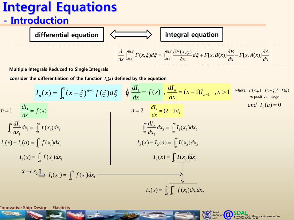
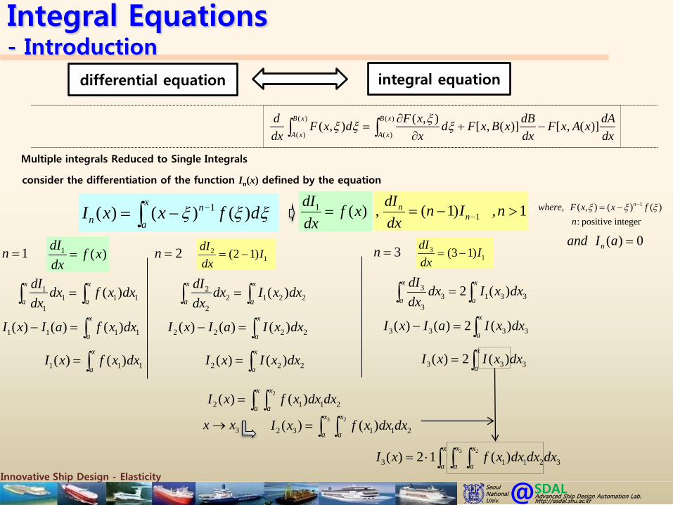
Multiple integrals Reduced to Single Integrals
( ) ( )
( ) ( )
( , )( , ) [ , ( )] [ , ( )]B x B x
A x A x
d F x dB dAF x d d F x B x F x A xdx x dx dx
ξξ ξ ξ∂= + −
∂∫ ∫
1( ) ( ) ( )x n
n aI x x f dξ ξ ξ−= −∫
consider the differentiation of the function In(x) defined by the equation
1, ( , ) ( ) ( ): positive integer
nwhere F x x fn
ξ ξ ξ−= −
1( ) ( )x nn
a
dI d x f ddx dx
ξ ξ ξ−= −∫differentiation with respect to x
2 1( 1) ( ) ( ) ( ) ( )x n n
xan x f d x f
ξξ ξ ξ ξ ξ− −
= = − − + − ∫
1 1 1( ) ( ) ( ) ( ) ( ) ( )x n n n
x aa
dx dax f d x f x fx dx dxξ ξ
ξ ξ ξ ξ ξ ξ ξ− − −
= =
∂ = − + − − − ∂∫01
integral equationdifferential equation

Innovative Ship Design - ElasticitySDAL@Advanced Ship Design Automation Lab.http://asdal.snu.ac.kr
Seoul NationalUniv.
Integral Equations- Introduction
Multiple integrals Reduced to Single Integrals
( ) ( )
( ) ( )
( , )( , ) [ , ( )] [ , ( )]B x B x
A x A x
d F x dB dAF x d d F x B x F x A xdx x dx dx
ξξ ξ ξ∂= + −
∂∫ ∫
1( ) ( ) ( )x n
n aI x x f dξ ξ ξ−= −∫
consider the differentiation of the function In(x) defined by the equation
1, ( , ) ( ) ( ): positive integer
nwhere F x x fn
ξ ξ ξ−= −
1( ) ( )x nn
a
dI d x f ddx dx
ξ ξ ξ−= −∫differentiation with respect to x
2 1( 1) ( ) ( ) ( ) ( )x n n
xan x f d x f
ξξ ξ ξ ξ ξ− −
= = − − + − ∫
1( 1) , 1nn
dI n I ndx −∴ = − >
Hence, if n>1, there follows While if n=1, we have
1 ( )dI f xdx
∴ =
2 1( 1) ( ) ( ) ( ) ( )x n nn
xa
dI n x f d x fdx ξ
ξ ξ ξ ξ ξ− −
= = − − + − ∫
02 1( 1) ( ) ( ) ( ) ( )
x n nnxa
dI n x f d x fdx ξ
ξ ξ ξ ξ ξ− −
= = − − + − ∫
0
1) Donald E. Knuth, Two notes on notation, Amer. Math. Monthly 99 no. 5 (May 1992), 403–422, see also http://en.wikipedia.org/wiki/Exponentiation
0 1)0 1=
integral equationdifferential equation
Innovative Ship Design - ElasticitySDAL@Advanced Ship Design Automation Lab.http://asdal.snu.ac.kr
Seoul NationalUniv.
Integral Equations- Introduction
Multiple integrals Reduced to Single Integrals
( ) ( )
( ) ( )
( , )( , ) [ , ( )] [ , ( )]B x B x
A x A x
d F x dB dAF x d d F x B x F x A xdx x dx dx
ξξ ξ ξ∂= + −
∂∫ ∫
1( ) ( ) ( )x n
n aI x x f dξ ξ ξ−= −∫
consider the differentiation of the function In(x) defined by the equation
1, ( , ) ( ) ( ): positive integer
nwhere F x x fn
ξ ξ ξ−= −1, ( 1) , 1n
ndI n I ndx −= − >1 ( )dI f x
dx=
1 ( )dI f xdx
=
11 1 1
1
( )x x
a a
dI dx f x dxdx
=∫ ∫
1 1 1 1( ) ( ) ( )x
aI x I a f x dx− = ∫
( ) 0nand I a =
1 1 1( ) ( )x
aI x f x dx= ∫
21(2 1)dI I
dx= −
22 1 2 2
2
( )x x
a a
dI dx I x dxdx
=∫ ∫
2 2 2 2( ) ( ) ( )x
aI x I a I x dx− = ∫
2 2 2( ) ( )x
aI x I x dx= ∫
2
2 1 1 2( ) ( )x x
a aI x f x dx dx= ∫ ∫
2
1 2 1 1( ) ( )x
aI x f x dx= ∫
1n = 2n =
2x x→
integral equationdifferential equation
Innovative Ship Design - ElasticitySDAL@Advanced Ship Design Automation Lab.http://asdal.snu.ac.kr
Seoul NationalUniv.
Integral Equations- Introduction
Multiple integrals Reduced to Single Integrals
( ) ( )
( ) ( )
( , )( , ) [ , ( )] [ , ( )]B x B x
A x A x
d F x dB dAF x d d F x B x F x A xdx x dx dx
ξξ ξ ξ∂= + −
∂∫ ∫
1( ) ( ) ( )x n
n aI x x f dξ ξ ξ−= −∫
consider the differentiation of the function In(x) defined by the equation
1, ( , ) ( ) ( ): positive integer
nwhere F x x fn
ξ ξ ξ−= −1, ( 1) , 1n
ndI n I ndx −= − >1 ( )dI f x
dx=
1 ( )dI f xdx
=
11 1 1
1
( )x x
a a
dI dx f x dxdx
=∫ ∫
1 1 1 1( ) ( ) ( )x
aI x I a f x dx− = ∫
( ) 0nand I a =
1 1 1( ) ( )x
aI x f x dx= ∫
21(2 1)dI I
dx= −
22 1 2 2
2
( )x x
a a
dI dx I x dxdx
=∫ ∫
2 2 2 2( ) ( ) ( )x
aI x I a I x dx− = ∫
2 2 2( ) ( )x
aI x I x dx= ∫
2
2 1 1 2( ) ( )x x
a aI x f x dx dx= ∫ ∫
1n = 2n = 31(3 1)dI I
dx= −
33 1 3 3
3
2 ( )x x
a a
dI dx I x dxdx
=∫ ∫
3 3 3 3( ) ( ) 2 ( )x
aI x I a I x dx− = ∫
3 3 3( ) 2 ( )x
aI x I x dx= ∫
3n =
3 2
3 1 1 2 3( ) 2 1 ( )x x x
a a aI x f x dx dx dx= ⋅ ∫ ∫ ∫
3 2
2 3 1 1 2( ) ( )x x
a aI x f x dx dx= ∫ ∫3x x→
integral equationdifferential equation

Innovative Ship Design - ElasticitySDAL@Advanced Ship Design Automation Lab.http://asdal.snu.ac.kr
Seoul NationalUniv.
Integral Equations- Introduction
Multiple integrals Reduced to Single Integrals
( ) ( )
( ) ( )
( , )( , ) [ , ( )] [ , ( )]B x B x
A x A x
d F x dB dAF x d d F x B x F x A xdx x dx dx
ξξ ξ ξ∂= + −
∂∫ ∫
1( ) ( ) ( )x n
n aI x x f dξ ξ ξ−= −∫
consider the differentiation of the function In(x) defined by the equation
1, ( , ) ( ) ( ): positive integer
nwhere F x x fn
ξ ξ ξ−= −
1, ( 1) , 1nn
dI n I ndx −= − >1 ( )dI f x
dx=
( ) 0nand I a =
1 ( )dI f xdx
=
11 1 1
1
( )x x
a a
dI dx f x dxdx
=∫ ∫
1 1 1 1( ) ( ) ( )x
aI x I a f x dx− = ∫
1 1 1( ) ( )x
aI x f x dx= ∫
21(2 1)dI I
dx= −
22 1 2 2
2
( )x x
a a
dI dx I x dxdx
=∫ ∫
2 2 2 2( ) ( ) ( )x
aI x I a I x dx− = ∫
2 2 2( ) ( )x
aI x I x dx= ∫
2
2 1 1 2( ) ( )x x
a aI x f x dx dx= ∫ ∫
1n = 2n = 31(3 1)dI I
dx= −
33 1 3 3
3
2 ( )x x
a a
dI dx I x dxdx
=∫ ∫
3 3 3 3( ) ( ) 2 ( )x
aI x I a I x dx− = ∫
3 3 3( ) 2 ( )x
aI x I x dx= ∫
3n =
3 2
3 1 1 2 3( ) 2 1 ( )x x x
a a aI x f x dx dx dx= ⋅ ∫ ∫ ∫
3 2
1 1 2 1( ) ( 1)! ( )nx x x x
n n na a a aI x n f x dx dx dx dx−= − ∫ ∫ ∫ ∫
integral equationdifferential equation

Innovative Ship Design - ElasticitySDAL@Advanced Ship Design Automation Lab.http://asdal.snu.ac.kr
Seoul NationalUniv.
Integral Equations- Introduction
Multiple integrals Reduced to Single Integrals
( ) ( )
( ) ( )
( , )( , ) [ , ( )] [ , ( )]B x B x
A x A x
d F x dB dAF x d d F x B x F x A xdx x dx dx
ξξ ξ ξ∂= + −
∂∫ ∫
1( ) ( ) ( )x n
n aI x x f dξ ξ ξ−= −∫
consider the differentiation of the function In(x) defined by the equation
1, ( , ) ( ) ( ): positive integer
nwhere F x x fn
ξ ξ ξ−= −
1, ( 1) , 1nn
dI n I ndx −= − >1 ( )dI f x
dx=
( ) 0nand I a =
3 2
1 1 2 1( ) ( 1)! ( )nx x x x
n n na a a aI x n f x dx dx dx dx−= − ∫ ∫ ∫ ∫
3 2
1 1 2 11( ) ( )
( 1)!nx x x x
n n na a a af x dx dx dx dx I x
n− =−∫ ∫ ∫ ∫
3 2 11 1 2 1
1( ) ( ) ( )( 1)!
nx x x x x nn na a a a a
f x dx dx dx dx x f dn
ξ ξ ξ−− = −
−∫ ∫ ∫ ∫ ∫
integral equationdifferential equation

Innovative Ship Design - ElasticitySDAL@Advanced Ship Design Automation Lab.http://asdal.snu.ac.kr
Seoul NationalUniv.
Integral Equations- Introduction
Multiple integrals Reduced to Single Integrals
( ) ( )
( ) ( )
( , )( , ) [ , ( )] [ , ( )]B x B x
A x A x
d F x dB dAF x d d F x B x F x A xdx x dx dx
ξξ ξ ξ∂= + −
∂∫ ∫
1( ) ( ) ( )x n
n aI x x f dξ ξ ξ−= −∫
consider the differentiation of the function In(x) defined by the equation
1, ( , ) ( ) ( ): positive integer
nwhere F x x fn
ξ ξ ξ−= −
3 2 11 1 2 1
1( ) ( ) ( )( 1)!
nx x x x x nn na a a a a
f x dx dx dx dx x f dn
ξ ξ ξ−− = −
−∫ ∫ ∫ ∫ ∫
What do you think the meaning of this equation is?
1) if you have a function f
2) and integrate it n times 3) you have this
integral equationdifferential equation
Innovative Ship Design - ElasticitySDAL@Advanced Ship Design Automation Lab.http://asdal.snu.ac.kr
Seoul NationalUniv.
Integral Equations : Relation between differential and integral equations

Innovative Ship Design - ElasticitySDAL@Advanced Ship Design Automation Lab.http://asdal.snu.ac.kr
Seoul NationalUniv.
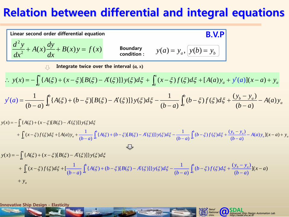
Relation between differential and integral equations
Linear second order differential equation
2
2 ( ) ( ) ( )d y dyA x B x y f xdx dx
+ + =0 0( ) , ( )y a y y a y′ ′= =
1 1 1 1 1 1 1 1 1 1( ) ( ) ( ) ( ) ( ) ( )x x x x
a a a ay x dx A x y x dx B x y x dx f x dx′′ ′+ + =∫ ∫ ∫ ∫
Initial condition :
Integrate with respect to x1 over the interval (a, x)
[ ]1 1 1 1 1 1 1 1 1( ) ( ) ( ) ( ) ( ) ( )x x xx
a a a ay x A x y x dx B x y x dx f x dx′ ′+ + =∫ ∫ ∫
1 1 1 1 1 1 1 1( ) ( ) ( ) ( ) ( ) ( ) ( )x x x
a a ay x y a A x y x dx B x y x dx f x dx′ ′ ′− = − − +∫ ∫ ∫
after integrating the first term on the right by parts,
[ ]1 1 1 1 1 1 1 1 1 1 0( ) ( ) ( ) ( ) ( ) ( ) ( ) ( )x x xx
a a a ay x A x y x A x y x dx B x y x dx f x dx y′ ′ ′= − + − + +∫ ∫ ∫
[ ]1 1 1 1 1 1 0( ) ( ) ( ) ( ) ( ) ( ) ( ) ( ) ( )x x
a ay x A x y x A a y a B x A x y x dx f x dx y′ ′ ′= − + − − + +∫ ∫
1 1 1 1 1 1 0 0( ) ( ) ( ) [ ( ) ( )] ( ) ( ) ( )x x
a ay x A x y x B x A x y x dx f x dx A a y y′ ′ ′= − − − + + +∫ ∫
0 1 1 1 1 1 1 1 1( ) ( ) ( ) ( ) ( ) ( )x x x
a a ay x y A x y x dx B x y x dx f x dx′ ′ ′− = − − +∫ ∫ ∫
I.V.P

Innovative Ship Design - ElasticitySDAL@Advanced Ship Design Automation Lab.http://asdal.snu.ac.kr
Seoul NationalUniv.
Relation between differential and integral equations
Linear second order differential equation
2
2 ( ) ( ) ( )d y dyA x B x y f xdx dx
+ + =0 0( ) , ( )y a y y a y′ ′= =Initial condition :
1 1 1 1 1 1 0 0( ) ( ) ( ) [ ( ) ( )] ( ) ( ) ( )x x
a ay x A x y x B x A x y x dx f x dx A a y y′ ′ ′= − − − + + +∫ ∫
( ){ }2 2 1 1 1 1 1 1 0 0 2( ) ( ) ( ) [ ( ) ( )] ( ) ( ) ( )x x x x
a a a ay x dx A x y x B x A x y x dx f x dx A a y y dx′ ′ ′= − − − + + +∫ ∫ ∫ ∫Integrate again over the interval (a, x)
( )[ ]2 2
1 1 1 1 1 1 1 2 1 1 2 0 0 2( ) ( ) ( ) ( ) [ ( ) ( )] ( ) ( ) ( )x x x x x x
aa a a ay x y a A x y x dx B x A x y x dx dx f x dx dx A a y y x′ ′− = − − − + + +∫ ∫ ∫ ∫ ∫
( )2 2
0 1 1 1 1 1 1 1 2 1 1 2 0 0( ) ( ) ( ) [ ( ) ( )] ( ) ( ) ( ) ( )x x x x x
a a a ay x y A x y x dx B x A x y x dx dx f x dx dx A a y y x a′ ′− = − − − + + + −∫ ∫ ∫ ∫ ∫
I.V.P

Innovative Ship Design - ElasticitySDAL@Advanced Ship Design Automation Lab.http://asdal.snu.ac.kr
Seoul NationalUniv.
Relation between differential and integral equations
Linear second order differential equation
2
2 ( ) ( ) ( )d y dyA x B x y f xdx dx
+ + =0 0( ) , ( )y a y y a y′ ′= =Initial condition :
Integrate twice over the interval (a, x)
( )2 2
0 1 1 1 1 1 1 1 2 1 1 2 0 0( ) ( ) ( ) [ ( ) ( )] ( ) ( ) ( ) ( )x x x x x
a a a a ay x y A x y x dx B x A x y x dx dx f x dx dx A a y y x a′ ′− = − − − + + + −∫ ∫ ∫ ∫ ∫
3 2 11 1 2 1
1( ) ( ) ( )( 1)!
nx x x x x nn na a a a a
f x dx dx dx dx x f dn
ξ ξ ξ−− = −
−∫ ∫ ∫ ∫ ∫
recall,
2 2 11 1 2
1( ) ( ) ( )(2 1)!
x x x
a a af x dx dx x f dξ ξ ξ−= −
−∫ ∫ ∫and for n=2
2
1 1 2( ) ( ) ( )x x x
a a af x dx dx x f dξ ξ ξ∴ = −∫ ∫ ∫
0 0 0( ) ( ) ( ) ( )[ ( ) ( )] ( ) ( ) ( ) [ ( ) ]( )x x x
a a ay x A y d x B A y d x f d A a y y x a yξ ξ ξ ξ ξ ξ ξ ξ ξ ξ ξ′ ′= − − − − + − + + − +∫ ∫ ∫
0 0 0( ) { ( ) ( )[ ( ) ( )]} ( ) ( ) ( ) [ ( ) ]( )x x
a ay x A x B A y d x f d A a y y x a yξ ξ ξ ξ ξ ξ ξ ξ ξ′ ′∴ = − + − − + − + + − +∫ ∫
I.V.P

Innovative Ship Design - ElasticitySDAL@Advanced Ship Design Automation Lab.http://asdal.snu.ac.kr
Seoul NationalUniv.
Relation between differential and integral equations
Linear second order differential equation
2
2 ( ) ( ) ( )d y dyA x B x y f xdx dx
+ + =0 0( ) , ( )y a y y a y′ ′= =Initial condition :
Integrate twice over the interval (a, x)
0 0 0( ) { ( ) ( )[ ( ) ( )]} ( ) ( ) ( ) [ ( ) ]( )x x
a ay x A x B A y d x f d A a y y x a yξ ξ ξ ξ ξ ξ ξ ξ ξ′ ′= − + − − + − + + − +∫ ∫
( ) ( , ) ( ) ( ),x
ay x K x y d F xξ ξ ξ= +∫ Where, ( , ) ( )[ ( ) ( )] ( )K x x B A Aξ ξ ξ ξ ξ′= − − −
0 0 0( ) ( ) ( ) [ ( ) ]( )x
aF x x f d A a y y x a yξ ξ ξ ′= − + + − +∫
This equation is seen to be a Volterra equation of the second kind.
: a linear function of the current variable x.
I.V.P
Innovative Ship Design - ElasticitySDAL@Advanced Ship Design Automation Lab.http://asdal.snu.ac.kr
Seoul NationalUniv.
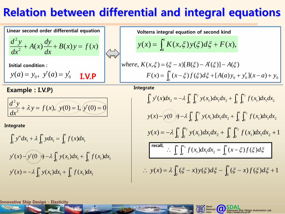
Relation between differential and integral equationsLinear second order differential equation
2
2 ( ) ( ) ( )d y dyA x B x y f xdx dx
+ + =
0 0( ) , ( )y a y y a y′ ′= =Initial condition :
( ) ( , ) ( ) ( ),x
ay x K x y d F xξ ξ ξ= +∫, ( , ) ( )[ ( ) ( )] ( )where K x x B A Aξ ξ ξ ξ ξ′= − − −
0 0 0( ) ( ) ( ) [ ( ) ]( )x
aF x x f d A a y y x a yξ ξ ξ ′= − + + − +∫
Volterra integral equation of second kind
2
2 ( ), (0) 1, (0) 0d y y f x y ydx
λ ′+ = = =
Example : I.V.P)
1 1 10 0 0( )
x x xy dx ydx f x dxλ′′ + =∫ ∫ ∫
1 1 1 10 0( ) (0 ) ( ) ( )
x xy x y y x dx f x dxλ′ ′− = − +∫ ∫
1 1 1 10 0( ) ( ) ( )
x xy x y x dx f x dxλ′ = − +∫ ∫
2 2
2 1 1 2 1 1 20 0 0 0 0( ) ( ) ( )
x x x x xy x dx y x dx dx f x dx dxλ′ = − +∫ ∫ ∫ ∫ ∫
0 0( ) ( ) ( ) ( ) ( ) 1
x xy x x y d x f dλ ξ ξ ξ ξ ξ ξ∴ = − − − +∫ ∫
2 2
1 1 2 1 1 20 0 0 0( ) (0 ) ( ) ( )
x x x xy x y y x dx dx f x dx dxλ− = − +∫ ∫ ∫ ∫
recall, 2
1 1 2( ) ( ) ( )x x x
a a af x dx dx x f dξ ξ ξ∴ = −∫ ∫ ∫
2 2
1 1 2 1 1 20 0 0 0( ) ( ) ( ) 1
x x x xy x y x dx dx f x dx dxλ= − + +∫ ∫ ∫ ∫
Integrate
Integrate
I.V.P

Innovative Ship Design - ElasticitySDAL@Advanced Ship Design Automation Lab.http://asdal.snu.ac.kr
Seoul NationalUniv.
Relation between differential and integral equationsLinear second order differential equation
2
2 ( ) ( ) ( )d y dyA x B x y f xdx dx
+ + =
0 0( ) , ( )y a y y a y′ ′= =Initial condition :
( ) ( , ) ( ) ( ),x
ay x K x y d F xξ ξ ξ= +∫, ( , ) ( )[ ( ) ( )] ( )where K x x B A Aξ ξ ξ ξ ξ′= − − −
0 0 0( ) ( ) ( ) [ ( ) ]( )x
aF x x f d A a y y x a yξ ξ ξ ′= − + + − +∫
Volterra integral equation of second kind
2
2 ( ), (0) 1, (0) 0d y y f x y ydx
λ ′+ = = =
Example : I.V.P)
0 0( ) ( ) ( ) ( ) ( ) 1
x xy x x y d x f dλ ξ ξ ξ ξ ξ ξ= − − − +∫ ∫
I.V.P
( ) 0, ( )A x B x λ= =
( , ) ( )[ ( ) ( )] ( )K x x B A Aξ ξ ξ ξ ξ′= − − −
( ) ( ) 1x
ax f dξ ξ ξ= − − +∫
0 0, 1, 0y y′= =
( ) ( , ) ( ) ( ),x
ay x K x y d F xξ ξ ξ= +∫
( )xλ ξ= −
0 0 0( ) ( ) ( ) [ ( ) ]( )x
aF x x f d A a y y x a yξ ξ ξ ′= − + + − +∫
check!

Innovative Ship Design - ElasticitySDAL@Advanced Ship Design Automation Lab.http://asdal.snu.ac.kr
Seoul NationalUniv.
Relation between differential and integral equations
Linear second order differential equation
2
2 ( ) ( ) ( )d y dyA x B x y f xdx dx
+ + = ( ) , ( )a by a y y b y= =
1 1 1 1 1 1 1 1 1 1( ) ( ) ( ) ( ) ( ) ( )x x x x
a a a ay x dx A x y x dx B x y x dx f x dx′′ ′+ + =∫ ∫ ∫ ∫
Boundary condition :
Integrate with respect to x1 over the interval (a, x)
[ ]1 1 1 1 1 1 1 1 1( ) ( ) ( ) ( ) ( ) ( )x x xx
a a a ay x A x y x dx B x y x dx f x dx′ ′+ + =∫ ∫ ∫
1 1 1 1 1 1 1 1( ) ( ) ( ) ( ) ( ) ( ) ( )x x x
a a ay x y a A x y x dx B x y x dx f x dx′ ′ ′− + + =∫ ∫ ∫
after integrating the first term on the right by parts,
[ ]1 1 1 1 1 1 1 1 1 1( ) ( ) ( ) ( ) ( ) ( ) ( ) ( ) ( )x x xx
a a a ay x A x y x A x y x dx B x y x dx f x dx y a′ ′ ′= − + − + +∫ ∫ ∫
[ ]1 1 1 1 1 1( ) ( ) ( ) ( ) ( ) ( ) ( ) ( ) ( ) ( )x x
a ay x A x y x A a y a B x A x y x dx f x dx y a′ ′ ′= − + − − + +∫ ∫
1 1 1 1 1 1( ) ( ) ( ) [ ( ) ( )] ( ) ( ) ( ) ( )x x
aa ay x A x y x B x A x y x dx f x dx A a y y a′ ′ ′= − − − + + +∫ ∫
1 1 1 1 1 1 1 1( ) ( ) ( ) ( ) ( ) ( ) ( )x x x
a a ay x y a A x y x dx B x y x dx f x dx′ ′ ′− = − − +∫ ∫ ∫
B.V.P

Innovative Ship Design - ElasticitySDAL@Advanced Ship Design Automation Lab.http://asdal.snu.ac.kr
Seoul NationalUniv.
Relation between differential and integral equations
Linear second order differential equation
2
2 ( ) ( ) ( )d y dyA x B x y f xdx dx
+ + = Boundary condition :
1 1 1 1 1 1( ) ( ) ( ) [ ( ) ( )] ( ) ( ) ( ) ( )x x
aa ay x A x y x B x A x y x dx f x dx A a y y a′ ′ ′= − − − + + +∫ ∫
( ){ }2 2 1 1 1 1 1 1 2( ) ( ) ( ) [ ( ) ( )] ( ) ( ) ( ) ( )x x x x
aa a a ay x dx A x y x B x A x y x dx f x dx A a y y a dx′ ′ ′= − − − + + +∫ ∫ ∫ ∫
Integrate again over the interval (a, x)
( )[ ]2 2
1 1 1 1 1 1 1 2 1 1 2 2( ) ( ) ( ) ( ) [ ( ) ( )] ( ) ( ) ( ) ( )x x x x x x
a aa a a a ay x y a A x y x dx B x A x y x dx dx f x dx dx A a y y a x′ ′− = − − − + + +∫ ∫ ∫ ∫ ∫
( )2 2
1 1 1 1 1 1 1 2 1 1 2( ) ( ) ( ) [ ( ) ( )] ( ) ( ) ( ) ( ) ( )x x x x x
a aa a a a ay x y A x y x dx B x A x y x dx dx f x dx dx A a y y a x a′ ′− = − − − + + + −∫ ∫ ∫ ∫ ∫
( ) , ( )a by a y y b y= =
B.V.P

Innovative Ship Design - ElasticitySDAL@Advanced Ship Design Automation Lab.http://asdal.snu.ac.kr
Seoul NationalUniv.
Relation between differential and integral equations
Linear second order differential equation
2
2 ( ) ( ) ( )d y dyA x B x y f xdx dx
+ + =
Integrate twice over the interval (a, x)
( )2 2
1 1 1 1 1 1 1 2 1 1 2( ) ( ) ( ) [ ( ) ( )] ( ) ( ) ( ) ( ) ( )x x x x x
a aa a a a ay x y A x y x dx B x A x y x dx dx f x dx dx A a y y a x a′ ′− = − − − + + + −∫ ∫ ∫ ∫ ∫
3 2 11 1 2 1
1( ) ( ) ( )( 1)!
nx x x x x nn na a a a a
f x dx dx dx dx x f dn
ξ ξ ξ−− = −
−∫ ∫ ∫ ∫ ∫
recall,
2 2 11 1 2
1( ) ( ) ( )(2 1)!
x x x
a a af x dx dx x f dξ ξ ξ−= −
−∫ ∫ ∫and for n=2
2
1 1 2( ) ( ) ( )x x x
a a af x dx dx x f dξ ξ ξ∴ = −∫ ∫ ∫
( ) ( ) ( ) ( )[ ( ) ( )] ( ) ( ) ( ) [ ( ) ( )]( )x x x
a aa a ay x A y d x B A y d x f d A a y y a x a yξ ξ ξ ξ ξ ξ ξ ξ ξ ξ ξ′ ′= − − − − + − + + − +∫ ∫ ∫
( ) { ( ) ( )[ ( ) ( )]} ( ) ( ) ( ) [ ( ) ( )]( )x x
a aa ay x A x B A y d x f d A a y y a x a yξ ξ ξ ξ ξ ξ ξ ξ ξ′ ′∴ = − + − − + − + + − +∫ ∫
( ) , ( )a by a y y b y= =
B.V.P
Boundary condition :

Innovative Ship Design - ElasticitySDAL@Advanced Ship Design Automation Lab.http://asdal.snu.ac.kr
Seoul NationalUniv.
Relation between differential and integral equations
Linear second order differential equation
2
2 ( ) ( ) ( )d y dyA x B x y f xdx dx
+ + =
Integrate twice over the interval (a, x)
( ) { ( ) ( )[ ( ) ( )]} ( ) ( ) ( ) [ ( ) ( )]( )x x
a aa ay x A x B A y d x f d A a y y a x a yξ ξ ξ ξ ξ ξ ξ ξ ξ′∴ = − + − − + − + −′+ +∫ ∫
( ) { ( ) ( )[ ( ) ( )]} ( ) ( ) ( ) [ ( ) ( )]( )b b
a aa ayy b A b B A y d b f d A a y b a yaξ ξ ξ ξ ξ ξ ξ ξ ξ′= − + − − + − ′+ + − +∫ ∫
( ) , ( )a by a y y b y= =
{ ( ) ( )[ ( ) ( )]} ( ) ( ) ( ) [ ( ) (( )] )b b
b a aa ay A b B A y d b f d A a y b yy a aξ ξ ξ ξ ξ ξ ξ ξ ξ′= − + − − + ′− + + − +∫ ∫
[ ( ) ]( ) { ( ) ( )[ ( ) ( )]} ( ) ( ) ( )( ) ( )b b
a b aa aA a y b a A b B A y d b f d yy a yξ ξ ξ ξ ξ ξ ξ ξ ξ′+ − = + − − − − + −′ ∫ ∫
1 1 ( )( ) { ( ) ( )[ ( ) ( )]} ( ) ( ) ( )( ) ( ) (
))
(b b b a
a a a
y yA a y A b B A y d b f db a b a b
y aa
ξ ξ ξ ξ ξ ξ ξ ξ ξ −′+ = + −′ − − − +− − −∫ ∫
1 1 ( ){ ( ) ( )[ ( ) ( )]} ( ) (( ) ( ) ( )( ) ( )
)( )
b b b aaa a
y yA b B A y d b f d A a yb a b a
aa
yb
ξ ξ ξ ξ ξ ξ ξ ξ ξ −′= + − − − − + −− − −
′ ∫ ∫
B.V.P
Boundary condition :
Innovative Ship Design - ElasticitySDAL@Advanced Ship Design Automation Lab.http://asdal.snu.ac.kr
Seoul NationalUniv.
Relation between differential and integral equations
Linear second order differential equation
2
2 ( ) ( ) ( )d y dyA x B x y f xdx dx
+ + =
Integrate twice over the interval (a, x)
( ) { ( ) ( )[ ( ) ( )]} ( ) ( ) ( ) [ ( ) ( )]( )x x
a aa ay x A x B A y d x f d A a y y a x a yξ ξ ξ ξ ξ ξ ξ ξ ξ′∴ = − + − − + − + −′+ +∫ ∫
( ) , ( )a by a y y b y= =
1 1 ( ){ ( ) ( )[ ( ) ( )]} ( ) (( ) ( ) ( )( ) ( )
)( )
b b b aaa a
y yA b B A y d b f d A a yb a b a
aa
yb
ξ ξ ξ ξ ξ ξ ξ ξ ξ −′= + − − − − + −− − −
′ ∫ ∫
( ) { ( ) ( )[ ( ) ( )]
1 1 ( ){ ( ) ( )[ ( ) ( )]} ( ) ( ) (
} ( )
( ) ( ) [ ( ) ( )( )
) ](
()
)) (
x
a
b b b aaa a
x
a aa
y yA b
y x A x
B A y d b f d A a yb a
B A y d
x fb a b
d A a a ya
y xξ ξ ξ ξ ξ ξ ξ
ξ ξ ξ ξ ξ ξ
ξ ξ ξ ξ ξ −′+ − − −
′= − + − −
+ − + − + −−
+−
+ −− ∫
∫
∫ ∫
( ) { ( ) ( )[ ( ) ( )]} ( )
1 1 ( ){ ( ) ( )[ ( ) ( )]} ( ) (( ) ( ) [ ]() ( )( (
)) ) ( )
b
x
a
x
a
a
b b aa a
y yA b
y x A x B A y d
B A yx f d xd b f db a b a b a
a
y
ξ ξ ξ ξ ξ
ξ ξ ξ ξ ξ
ξ
ξ ξ ξ ξ ξ ξ ξ
′= − + − −
+−′+ − − − −−
− −+
+−
+ −∫ ∫
∫
∫
B.V.P
Boundary condition :

Innovative Ship Design - ElasticitySDAL@Advanced Ship Design Automation Lab.http://asdal.snu.ac.kr
Seoul NationalUniv.
Relation between differential and integral equations
( ) { ( ) ( )[ ( ) ( )]} ( )
1 1 ( ){ ( ) ( )[ ( ) ( )]} ( ) (( ) ( ) [ ]() ( )( (
)) ) ( )
b
x
a
x
a
a
b b aa a
y yA b
y x A x B A y d
B A yx f d xd b f db a b a b a
a
y
ξ ξ ξ ξ ξ
ξ ξ ξ ξ ξ
ξ
ξ ξ ξ ξ ξ ξ ξ
′= − + − −
+−′+ − − − −−
− −+
+−
+ −∫ ∫
∫
∫
{ ( ) ( )[ ( ) ( )]} ( )( )( ) { ( ) ( )[ ( ) ( )]} ( )
( ) ( )( ) ( )
( )
( ) ( ) ( )( ) ( )
x b
aa
x b
aa baa
x ay x A x B A y d
x a x ax
A b B
f d y
A y db a
b f d y yb a b a
ξ ξ ξ ξ ξ ξξ ξ ξ ξ ξ ξ
ξ ξ ξ ξ ξ ξ
−′= ′+ − −−
− − + −− −
− + − − +
− −+ − +∫ ∫
∫ ∫1
2

Innovative Ship Design - ElasticitySDAL@Advanced Ship Design Automation Lab.http://asdal.snu.ac.kr
Seoul NationalUniv.
Relation between differential and integral equations
1
( ){ ( ) ( )[ ( ) ( )]} ( ) { ( ) ( )[ ( ) ( )]} ( )( )
( ) ( ){ ( ) ( )[ ( ) ( )]} ( ) { ( ) ( )[ ( ) ( )]} ( ) { ( ) ( )[ ( ) ( )]} ( )( ) ( )
x b
a a
x b
a a
x
x
x aA x B A y d A b B A y db a
x a x aA x B A y d A b B A y d A b B A y db a b a
ξ ξ ξ ξ ξ ξ ξ ξ ξ ξ ξ ξ
ξ ξ ξ ξ ξ ξ ξ ξ ξ ξ ξ ξ ξ ξ ξ ξ ξ ξ
−′ ′− + − − + + − −−− −′ ′ ′= − + − − + + − − + + − −− −
∫ ∫
∫ ∫( ) ( ) ( ){ ( ) 1 ( ) ( ) [ ( ) ( )]} ( ) { ( ) ( )[ ( ) ( )]} ( )( ) ( ) ( )
( )( ) ( )( ){ ( ) [ ( ) ( )]} ( )( ) ( )
x b
a x
x
a
x a x a x aA x b B A y d A b B A y db a b a b a
b a x a x b a x a bA B A y db a b a
ξ ξ ξ ξ ξ ξ ξ ξ ξ ξ ξ ξ ξ
ξ ξξ ξ ξ ξ ξ
− − −′ ′= − − + − − − − + + − − − − − − − + − − − − − ′= − + − − −
∫
∫ ∫
∫( ) { ( ) ( )[ ( ) ( )]} ( )( )( ){ ( ) [ ( ) ( )]} ( ) { ( ) ( )[ ( ) ( )]} ( )( )
{ ( )
b
x
x b
a x
x a A b B A y db a
b x xb xa b a xb x ab a x aA B A y d A b B A y db a b a b ab x xa b x abAb a b a
ξ ξ ξ ξ ξ ξ
ξ ξ ξ ξξ ξ ξ ξ ξ ξ ξ ξ ξ ξ ξ
ξ ξξ
− ′+ + − −−
− − − + − + + − − ′ ′= − + − + + − − − − − − − − + + = − + − −
∫
∫ ∫
[ ( ) ( )]} ( ) { ( ) ( ) [ ( ) ( )]} ( )
( ) ( ) ( )( ){ ( ) [ ( ) ( )]} ( ) { ( ) [ ( ) ( )]} (
x b
a x
x
a
x a x aB A y d A b B A y db a b a
b x a b x b x x a x a bA B A y d A B A yb a b a b a b a
ξ ξ ξ ξ ξ ξ ξ ξ ξ ξ
ξ ξξ ξ ξ ξ ξ ξ ξ ξ
− − ′ ′− + + − − − − − − − − − − − ′ ′= − + − + + − − − − −
∫ ∫
∫ )b
xdξ ξ∫
{ ( ) ( )[ ( ) ( )]} ( )( )( ) { ( ) ( )[ ( ) ( )]} ( )
( ) ( )( ) ( )
( )
( ) ( ) ( )( ) ( )
x b
aa
x b
aa baa
x ay x A x B A y d
x a x ax
A b B
f d y
A y db a
b f d y yb a b a
ξ ξ ξ ξ ξ ξξ ξ ξ ξ ξ ξ
ξ ξ ξ ξ ξ ξ
−′= ′+ − −−
− − + −− −
− + − − +
− −+ − +∫ ∫
∫ ∫1
2
Innovative Ship Design - ElasticitySDAL@Advanced Ship Design Automation Lab.http://asdal.snu.ac.kr
Seoul NationalUniv.
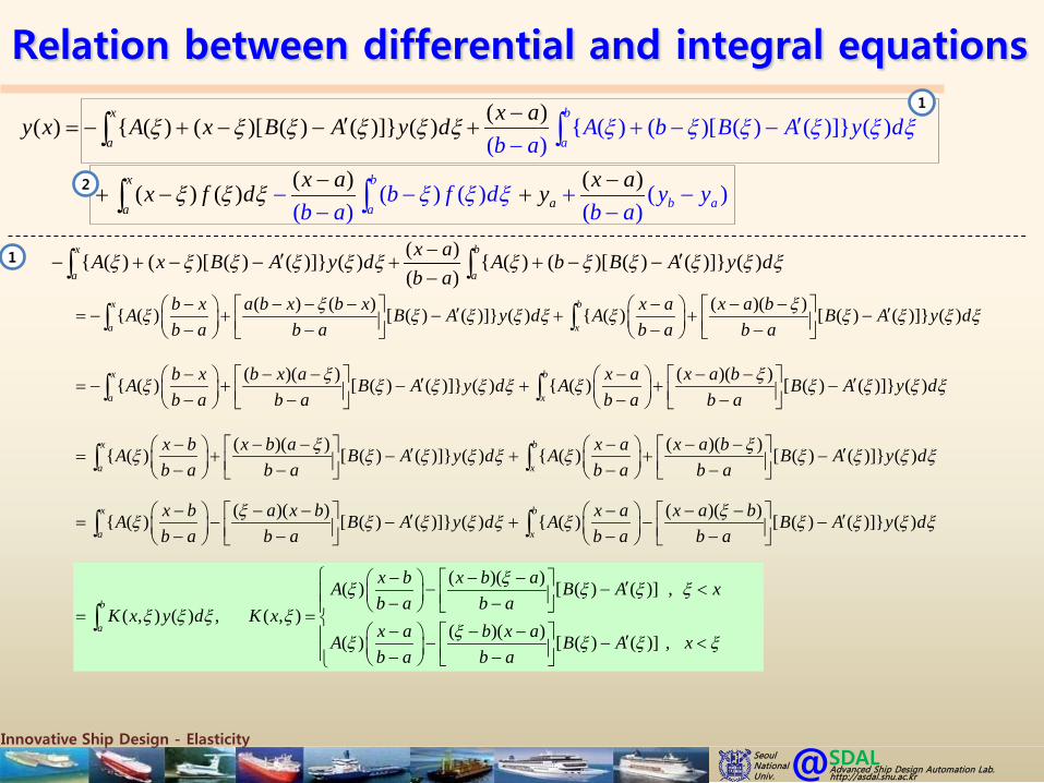
Relation between differential and integral equations
1
( )( ) ( )( ){ ( ) [ ( ) ( )]} ( ) { ( ) [ ( ) ( )]} ( )x b
a x
x b a x b x a x a bA B A y d A B A y db a b a b a b a
ξ ξξ ξ ξ ξ ξ ξ ξ ξ ξ ξ− − − − − − ′ ′= − − + − − − − − − ∫ ∫
( )( )( ) [ ( ) ( )] ,( , ) ( ) , ( , )
( )( )( ) [ ( ) ( )] ,
b
a
x b x b aA B A xb a b a
K x y d K xx a b x aA B A xb a b a
ξξ ξ ξ ξξ ξ ξ ξ
ξξ ξ ξ ξ
− − − ′− − < − − = = − − − ′− − < − −
∫
( ) ( ) ( )( ){ ( ) [ ( ) ( )]} ( ) { ( ) [ ( ) ( )]} ( )x b
a x
b x a b x b x x a x a bA B A y d A B A y db a b a b a b a
ξ ξξ ξ ξ ξ ξ ξ ξ ξ ξ ξ− − − − − − − ′ ′= − + − + + − − − − − ∫ ∫
( )( ) ( )( ){ ( ) [ ( ) ( )]} ( ) { ( ) [ ( ) ( )]} ( )x b
a x
b x b x a x a x a bA B A y d A B A y db a b a b a b a
ξ ξξ ξ ξ ξ ξ ξ ξ ξ ξ ξ− − − − − − ′ ′= − + − + + − − − − − ∫ ∫
( )( ) ( )( ){ ( ) [ ( ) ( )]} ( ) { ( ) [ ( ) ( )]} ( )x b
a x
x b x b a x a x a bA B A y d A B A y db a b a b a b a
ξ ξξ ξ ξ ξ ξ ξ ξ ξ ξ ξ− − − − − − ′ ′= + − + + − − − − − ∫ ∫
( ){ ( ) ( )[ ( ) ( )]} ( ) { ( ) ( )[ ( ) ( )]} ( )( )
x b
a a
x aA x B A y d A b B A y db a
ξ ξ ξ ξ ξ ξ ξ ξ ξ ξ ξ ξ−′ ′− + − − + + − −−∫ ∫
{ ( ) ( )[ ( ) ( )]} ( )( )( ) { ( ) ( )[ ( ) ( )]} ( )
( ) ( )( ) ( )
( )
( ) ( ) ( )( ) ( )
x b
aa
x b
aa baa
x ay x A x B A y d
x a x ax
A b B
f d y
A y db a
b f d y yb a b a
ξ ξ ξ ξ ξ ξξ ξ ξ ξ ξ ξ
ξ ξ ξ ξ ξ ξ
−′= ′+ − −−
− − + −− −
− + − − +
− −+ − +∫ ∫
∫ ∫1
2

Innovative Ship Design - ElasticitySDAL@Advanced Ship Design Automation Lab.http://asdal.snu.ac.kr
Seoul NationalUniv.
Relation between differential and integral equations
2 ( ) (( ) ( ) ( ))( ) ( )( ) ( )
x
a
b
b aaab fx a x ax f d yd y y
b a b aξ ξ ξξ ξ ξ − − +
−− −
− + −−∫ ∫
{ ( ) ( )[ ( ) ( )]} ( )( )( ) { ( ) ( )[ ( ) ( )]} ( )
( ) ( )( ) ( )
( )
( ) ( ) ( )( ) ( )
x b
aa
x b
aa baa
x ay x A x B A y d
x a x ax
A b B
f d y
A y db a
b f d y yb a b a
ξ ξ ξ ξ ξ ξξ ξ ξ ξ ξ ξ
ξ ξ ξ ξ ξ ξ
−′= ′+ − −−
− − + −− −
− + − − +
− −+ − +∫ ∫
∫ ∫1
2
( )( ) ( ) ( ) ( )x b
b a aa a
x ax f d y y b f d yb a
ξ ξ ξ ξ ξ ξ−= − + − − − +
−∫ ∫

Innovative Ship Design - ElasticitySDAL@Advanced Ship Design Automation Lab.http://asdal.snu.ac.kr
Seoul NationalUniv.
Relation between differential and integral equations
{ ( ) ( )[ ( ) ( )]} ( )( )( ) { ( ) ( )[ ( ) ( )]} ( )
( ) ( )( ) ( )
( )
( ) ( ) ( )( ) ( )
x b
aa
x b
aa baa
x ay x A x B A y d
x a x ax
A b B
f d y
A y db a
b f d y yb a b a
ξ ξ ξ ξ ξ ξξ ξ ξ ξ ξ ξ
ξ ξ ξ ξ ξ ξ
−′= ′+ − −−
− − + −− −
− + − − +
− −+ − +∫ ∫
∫ ∫1
2
1
( )( )( ) [ ( ) ( )] ,( , ) ( ) , ( , )
( )( )( ) [ ( ) ( )] ,
b
a
x b x b aA B A xb a b a
K x y d K xx a b x aA B A xb a b a
ξξ ξ ξ ξξ ξ ξ ξ
ξξ ξ ξ ξ
− − − ′− − < − − = − − − ′− − < − −
∫
2
( ) ( , ) ( ) ( ),b
ay x K x y d F xξ ξ ξ∴ = +∫
( )( ) ( ) ( ) ( )x b
b a aa a
x ax f d y y b f d yb a
ξ ξ ξ ξ ξ ξ−− + − − − +
−∫ ∫
( )
( )( )( ) [ ( ) ( )] ,, ( , )
( )( )( ) [ ( ) ( )] ,
, ( ) ( ) ( ) ( ) ( )x b
b a aa a
x b x b aA B A xb a b a
K xx a b x aA B A xb a b a
x aF x x f d y y b f d yb a
ξξ ξ ξ ξξ
ξξ ξ ξ ξ
ξ ξ ξ ξ ξ ξ
− − − ′− − < − − = − − − ′− − < − −
−= − + − − − +
−∫ ∫This equation is seen to be a Fredholmequation of the second kind.*
* Jerry, A.J., Introduction to Integral Equations with Applications, Marcel Dekker Inc., 1985, p67

Innovative Ship Design - ElasticitySDAL@Advanced Ship Design Automation Lab.http://asdal.snu.ac.kr
Seoul NationalUniv.
Relation between differential and integral equations
( )
( )( )( ) [ ( ) ( )] ,, ( , )
( )( )( ) [ ( ) ( )] ,
, ( ) ( ) ( ) ( ) ( )x b
b a aa a
x b x b aA B A xb a b a
K xx a b x aA B A xb a b a
x aF x x f d y y b f d yb a
ξξ ξ ξ ξξ
ξξ ξ ξ ξ
ξ ξ ξ ξ ξ ξ
− − − ′− − < − − = − − − ′− − < − −
−= − + − − − +
−∫ ∫
Linear second order differential equation2
2 ( ) ( ) ( )d y dyA x B x y f xdx dx
+ + =
Boundary condition :
( ) , ( )a by a y y b y= =
Fredholm equation of the second kind.
B.V.P( ) ( , ) ( ) ( ),
b
ay x K x y d F xξ ξ ξ= +∫
Example : Boundary Value Problem
2
2 0, (0) 0, ( ) 0d y y y y ldx
λ+ = = =
1 10 00
l ly dx ydxλ′′ + =∫ ∫
1 10( ) (0) ( )
xy x y y x dxλ′ ′− = − ∫
2 1 1 20 0 0( ) (0)
x x xy dx y x dx y dxλ ′ ′= − + ∫ ∫ ∫
2
1 1 2 10 0 0( ) (0) ( ) (0)
x x xy x y y x dx dx y dxλ ′− = − +∫ ∫ ∫
1 10 0
l ly dx ydxλ′′ = −∫ ∫
recall, 2
1 1 2( ) ( ) ( )x x x
a a af x dx dx x f dξ ξ ξ∴ = −∫ ∫ ∫
[ ]1 00( ) ( ) ( ) (0)
x xy x x y d y xλ ξ ξ ξ ′= − − +∫
0( ) ( ) ( ) (0)
xy x x y d y xλ ξ ξ ξ ′= − − + ⋅∫

Innovative Ship Design - ElasticitySDAL@Advanced Ship Design Automation Lab.http://asdal.snu.ac.kr
Seoul NationalUniv.
Relation between differential and integral equations
( )
( )( )( ) [ ( ) ( )] ,, ( , )
( )( )( ) [ ( ) ( )] ,
, ( ) ( ) ( ) ( ) ( )x b
b a aa a
x b x b aA B A xb a b a
K xx a b x aA B A xb a b a
x aF x x f d y y b f d yb a
ξξ ξ ξ ξξ
ξξ ξ ξ ξ
ξ ξ ξ ξ ξ ξ
− − − ′− − < − − = − − − ′− − < − −
−= − + − − − +
−∫ ∫
Linear second order differential equation2
2 ( ) ( ) ( )d y dyA x B x y f xdx dx
+ + =
Boundary condition :
( ) , ( )a by a y y b y= =
Fredholm equation of the second kind.
B.V.P( ) ( , ) ( ) ( ),
b
ay x K x y d F xξ ξ ξ= +∫
0( ) ( ) ( ) ( ) ( ) ( )
x
x
lx xy x x l y d l y dl l
λλ ξ ξ ξ ξ ξ ξ ξ = − − − − + − ∫ ∫
Example : Boundary Value Problem
2
2 0, (0) 0, ( ) 0d y y y y ldx
λ+ = = =
0( ) ( ) ( ) (0)
xy x x y d y xλ ξ ξ ξ ′= − − + ⋅∫
0( ) ( ) ( ) (0)
ly l l y d y lλ ξ ξ ξ ′= − − + ⋅∫
0(0) ( ) ( )
ly l y d
lλ ξ ξ ξ′∴ = −∫
0 0( ) ( ) ( ) ( ) ( )
x lxy x x y d l y dlλλ ξ ξ ξ ξ ξ ξ= − − + −∫ ∫
0( ) ( , ) ( )
ly x K x y dλ ξ ξ ξ∴ = ∫
0 0( ) ( ) ( ) ( ) ( ) ( ) ( )
x lx
x
x xy x x y d l y d l y dl lλ λλ ξ ξ ξ ξ ξ ξ ξ ξ ξ= − − + − + −∫ ∫ ∫
0( ) ( ) ( ) ( )
x l
x
x xy x y d l y dl l
λλ ξ ξ ξ ξ ξ ξ ξ = − − + + − ∫ ∫
0( ) ( )( ) ( ) ( )
x
x
l xl x ll
y x y d y dl
ξλ ξ ξ λ ξ ξξ= +− −∫ ∫0
0 ( ) ( ) (0)l
l y d y lλ ξ ξ ξ ′= − − + ⋅∫

Innovative Ship Design - ElasticitySDAL@Advanced Ship Design Automation Lab.http://asdal.snu.ac.kr
Seoul NationalUniv.
Relation between differential and integral equations
( )
( )( )( ) [ ( ) ( )] ,, ( , )
( )( )( ) [ ( ) ( )] ,
, ( ) ( ) ( ) ( ) ( )x b
b a aa a
x b x b aA B A xb a b a
K xx a b x aA B A xb a b a
x aF x x f d y y b f d yb a
ξξ ξ ξ ξξ
ξξ ξ ξ ξ
ξ ξ ξ ξ ξ ξ
− − − ′− − < − − = − − − ′− − < − −
−= − + − − − +
−∫ ∫
Linear second order differential equation2
2 ( ) ( ) ( )d y dyA x B x y f xdx dx
+ + =
Boundary condition :
( ) , ( )a by a y y b y= =
Fredholm equation of the second kind.
B.V.P( ) ( , ) ( ) ( ),
b
ay x K x y d F xξ ξ ξ= +∫
Example : Boundary Value Problem2
2 0, (0) 0, ( ) 0d y y y y ldx
λ+ = = =
0( ) ( , ) ( )
ly x K x y dλ ξ ξ ξ∴ = ∫
( ), ( , )
( )
l x when xlK xx l when xl
ξ ξξ
ξ ξ
− <= − >
( ) 0, , 0, 0, 0, ,( ) ( ) 0a bA x y y a b lB x f xλ= = = = == =check!
( ),( , )
( ),
l x xlK xx l xl
ξλ ξξ
λ ξ ξ
− <= − <
( ) 0F x =
( ) ( , ) ( )b
ay x K x y dξ ξ ξ∴ = ∫

Innovative Ship Design - ElasticitySDAL@Advanced Ship Design Automation Lab.http://asdal.snu.ac.kr
Seoul NationalUniv.
Relation between differential and integral equations
( )
( )( )( ) [ ( ) ( )] ,, ( , )
( )( )( ) [ ( ) ( )] ,
, ( ) ( ) ( ) ( ) ( )x b
b a aa a
x b x b aA B A xb a b a
K xx a b x aA B A xb a b a
x aF x x f d y y b f d yb a
ξξ ξ ξ ξξ
ξξ ξ ξ ξ
ξ ξ ξ ξ ξ ξ
− − − ′− − < − − = − − − ′− − < − −
−= − + − − − +
−∫ ∫
Linear second order differential equation2
2 ( ) ( ) ( )d y dyA x B x y f xdx dx
+ + =
Boundary condition :
( ) , ( )a by a y y b y= =
Fredholm equation of the second kind.
B.V.P( ) ( , ) ( ) ( ),
b
ay x K x y d F xξ ξ ξ= +∫
Example : Boundary Value Problem2
2 0, (0) 0, ( ) 0d y y y y ldx
λ+ = = =
0( ) ( , ) ( )
ly x K x y dλ ξ ξ ξ∴ = ∫
( ), ( , )
( )
l x when xlK xx l when xl
ξ ξξ
ξ ξ
− <= − >
•When does this mean?
from the example, by direct integration.
•What we had was2
2 ( ) ( ) ( )d y dyA x B x y f xdx dx
+ + =
in case o f ( ) 0, ( ) , ( ) 0A x B x f xλ= = =
•What we did is
•What we have is 0
( ) ( , ) ( )l
y x K x y dλ ξ ξ ξ= ∫we express y in terms of ‘Kernel’
( ), ( , )
( )
l x when xlK xx l when xl
ξ ξξ
ξ ξ
− <= − >
to transform D.E of B.V.P into I.E
if we find a ‘kernel’ of some properties, we can express y of a D.E as an ‘integral’ formwhich can be a solution or an equation
what kind of properties?
Innovative Ship Design - ElasticitySDAL@Advanced Ship Design Automation Lab.http://asdal.snu.ac.kr
Seoul NationalUniv.
Relation between differential and integral equations
( )
( )( )( ) [ ( ) ( )] ,, ( , )
( )( )( ) [ ( ) ( )] ,
, ( ) ( ) ( ) ( ) ( )x b
b a aa a
x b x b aA B A xb a b a
K xx a b x aA B A xb a b a
x aF x x f d y y b f d yb a
ξξ ξ ξ ξξ
ξξ ξ ξ ξ
ξ ξ ξ ξ ξ ξ
− − − ′− − < − − = − − − ′− − < − −
−= − + − − − +
−∫ ∫
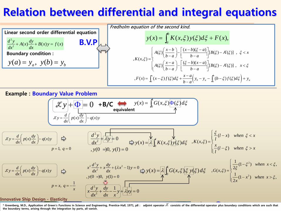
Linear second order differential equation2
2 ( ) ( ) ( )d y dyA x B x y f xdx dx
+ + =
Boundary condition :
( ) , ( )a by a y y b y= =
Fredholm equation of the second kind.
B.V.P( ) ( , ) ( ) ( ),
b
ay x K x y d F xξ ξ ξ= +∫
Example : Boundary Value Problem
2
2 0
, (0 )0, ( ) 0
d y ydxy y l
λ+ =
= =
( ), ( , )
( )
l x when xlK xx l when xl
ξ ξξ
ξ ξ
− <= − >
22 2
2 ( 1) 0
, (0 )0, (1) 0
d y dyx x x ydx dx
y y
λ+ + − =
= =
( ) ( )d dyy p x q x ydx dx
= −
L
2
2
1 (1 ) ,2, ( , )1 (1 ) ,
2
when xG x
x when xx
ξ ξξξ
ξ
− <= − >
0( ) ( , ) ( )
ly x K x y dλ ξ ξ ξ= ∫
1
0( ) ( , ) ( )y x G x y dλ ξ ξ ξ ξ= ∫
0y + Φ =L1
0( ) ( , ) ( )y x G x dξ ξ ξ= Φ∫+B/C
equivalent
2
2
1 0d y dyx y xydx dx x
λ+ − + =
*
* Greenberg, M.D., Application of Green’s Functions in Science and Engineering, Prentice-Hall, 1971, p8 : adjoint operator consists of the differential operator plus boundary conditions which are such that the boundary terms, arising through the integration by parts, all vanish.
1, 0p q= =
( ) ( )d dyy p x q x ydx dx
= −
L
1,p x qx
= = −
( ) ( )d dyy p x q x ydx dx
= −
L
L
Innovative Ship Design - ElasticitySDAL@Advanced Ship Design Automation Lab.http://asdal.snu.ac.kr
Seoul NationalUniv.
Relation between differential and integral equations
( )
( )( )( ) [ ( ) ( )] ,, ( , )
( )( )( ) [ ( ) ( )] ,
, ( ) ( ) ( ) ( ) ( )x b
b a aa a
x b x b aA B A xb a b a
K xx a b x aA B A xb a b a
x aF x x f d y y b f d yb a
ξξ ξ ξ ξξ
ξξ ξ ξ ξ
ξ ξ ξ ξ ξ ξ
− − − ′− − < − − = − − − ′− − < − −
−= − + − − − +
−∫ ∫
Linear second order differential equation2
2 ( ) ( ) ( )d y dyA x B x y f xdx dx
+ + =
Boundary condition :
( ) , ( )a by a y y b y= =
Fredholm equation of the second kind.
B.V.P( ) ( , ) ( ) ( ),
b
ay x K x y d F xξ ξ ξ= +∫
Example : Boundary Value Problem2
2 0, (0) 0, ( ) 0d y y y y ldx
λ+ = = =
0( ) ( , ) ( )
ly x K x y dλ ξ ξ ξ∴ = ∫
( ), ( , )
( )
l x when xlK xx l when xl
ξ ξξ
ξ ξ
− <= − >
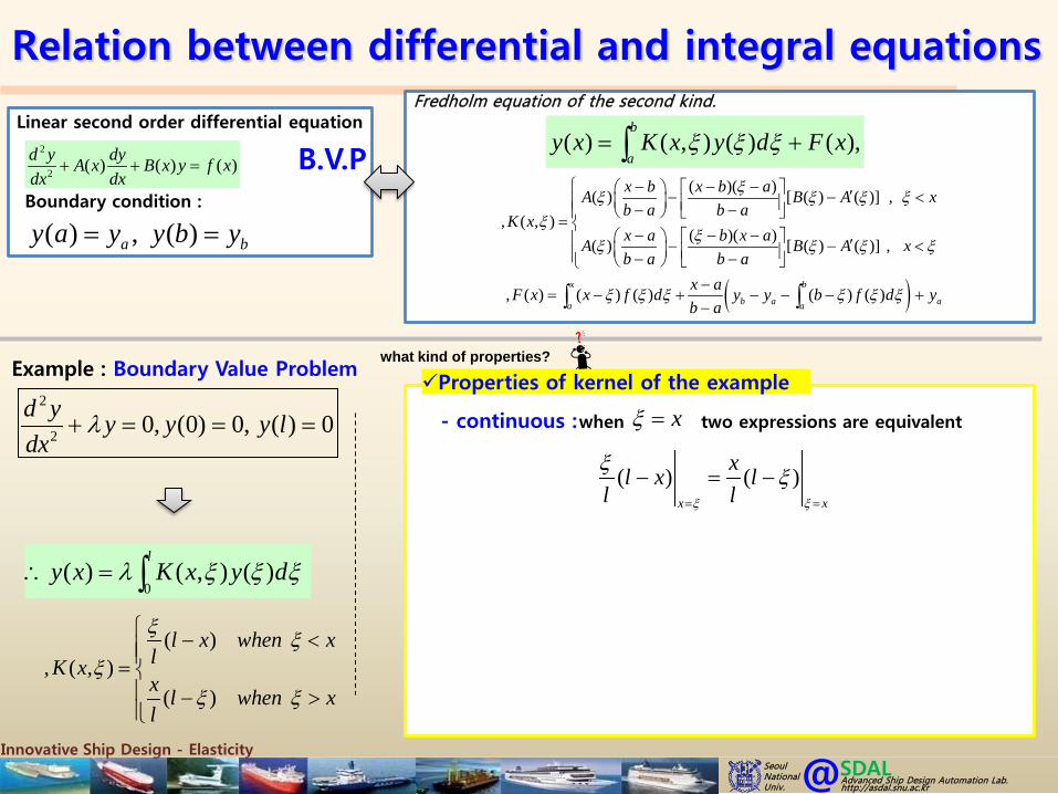
what kind of properties?
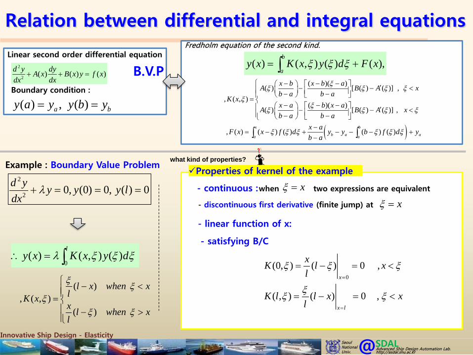
Properties of kernel of the example
when two expressions are equivalent- continuous : xξ =
( ) ( )x x
xl x ll lξ ξ
ξ ξ= =
− = −

Innovative Ship Design - ElasticitySDAL@Advanced Ship Design Automation Lab.http://asdal.snu.ac.kr
Seoul NationalUniv.
Relation between differential and integral equations
( )
( )( )( ) [ ( ) ( )] ,, ( , )
( )( )( ) [ ( ) ( )] ,
, ( ) ( ) ( ) ( ) ( )x b
b a aa a
x b x b aA B A xb a b a
K xx a b x aA B A xb a b a
x aF x x f d y y b f d yb a
ξξ ξ ξ ξξ
ξξ ξ ξ ξ
ξ ξ ξ ξ ξ ξ
− − − ′− − < − − = − − − ′− − < − −
−= − + − − − +
−∫ ∫
Linear second order differential equation2
2 ( ) ( ) ( )d y dyA x B x y f xdx dx
+ + =
Boundary condition :
( ) , ( )a by a y y b y= =
Fredholm equation of the second kind.
B.V.P( ) ( , ) ( ) ( ),
b
ay x K x y d F xξ ξ ξ= +∫
Example : Boundary Value Problem2
2 0, (0) 0, ( ) 0d y y y y ldx
λ+ = = =
0( ) ( , ) ( )
ly x K x y dλ ξ ξ ξ∴ = ∫
( ), ( , )
( )
l x when xlK xx l when xl
ξ ξξ
ξ ξ
− <= − >
what kind of properties?
when two expressions are equivalent- continuous : xξ =
- discontinuous first derivative (finite jump) at xξ =
( )
( ) 1
d l xdx l ld x ldx l l
ξ ξ
ξξ
− = − − = −
( ) ( ) 1 1d d xl x ldx l dx l l l
ξ ξ ξξ ∴ − − − = − − + = −
Properties of kernel of the example

Innovative Ship Design - ElasticitySDAL@Advanced Ship Design Automation Lab.http://asdal.snu.ac.kr
Seoul NationalUniv.
Relation between differential and integral equations
( )
( )( )( ) [ ( ) ( )] ,, ( , )
( )( )( ) [ ( ) ( )] ,
, ( ) ( ) ( ) ( ) ( )x b
b a aa a
x b x b aA B A xb a b a
K xx a b x aA B A xb a b a
x aF x x f d y y b f d yb a
ξξ ξ ξ ξξ
ξξ ξ ξ ξ
ξ ξ ξ ξ ξ ξ
− − − ′− − < − − = − − − ′− − < − −
−= − + − − − +
−∫ ∫
Linear second order differential equation2
2 ( ) ( ) ( )d y dyA x B x y f xdx dx
+ + =
Boundary condition :
( ) , ( )a by a y y b y= =
Fredholm equation of the second kind.
B.V.P( ) ( , ) ( ) ( ),
b
ay x K x y d F xξ ξ ξ= +∫
Example : Boundary Value Problem2
2 0, (0) 0, ( ) 0d y y y y ldx
λ+ = = =
0( ) ( , ) ( )
ly x K x y dλ ξ ξ ξ∴ = ∫
( ), ( , )
( )
l x when xlK xx l when xl
ξ ξξ
ξ ξ
− <= − >
what kind of properties?
when two expressions are equivalent- continuous : xξ =
- discontinuous first derivative (finite jump) at xξ =
2
2
( , ) 0K xx
ξ∂=
∂
- linear function of x:
Properties of kernel of the example
Innovative Ship Design - ElasticitySDAL@Advanced Ship Design Automation Lab.http://asdal.snu.ac.kr
Seoul NationalUniv.
Relation between differential and integral equations
( )
( )( )( ) [ ( ) ( )] ,, ( , )
( )( )( ) [ ( ) ( )] ,
, ( ) ( ) ( ) ( ) ( )x b
b a aa a
x b x b aA B A xb a b a
K xx a b x aA B A xb a b a
x aF x x f d y y b f d yb a
ξξ ξ ξ ξξ
ξξ ξ ξ ξ
ξ ξ ξ ξ ξ ξ
− − − ′− − < − − = − − − ′− − < − −
−= − + − − − +
−∫ ∫
Linear second order differential equation2
2 ( ) ( ) ( )d y dyA x B x y f xdx dx
+ + =
Boundary condition :
( ) , ( )a by a y y b y= =
Fredholm equation of the second kind.
B.V.P( ) ( , ) ( ) ( ),
b
ay x K x y d F xξ ξ ξ= +∫
Example : Boundary Value Problem2
2 0, (0) 0, ( ) 0d y y y y ldx
λ+ = = =
0( ) ( , ) ( )
ly x K x y dλ ξ ξ ξ∴ = ∫
( ), ( , )
( )
l x when xlK xx l when xl
ξ ξξ
ξ ξ
− <= − >
what kind of properties?
when two expressions are equivalent- continuous : xξ =
- discontinuous first derivative (finite jump) at xξ =
- linear function of x:
- satisfying B/C
0
(0, ) ( ) 0 ,
( , ) ( ) 0 ,
x
x l
xK l xl
K l l x xl
ξ ξ ξ
ξξ ξ
=
=
= − = <
= − = <
Properties of kernel of the example

Innovative Ship Design - ElasticitySDAL@Advanced Ship Design Automation Lab.http://asdal.snu.ac.kr
Seoul NationalUniv.
Relation between differential and integral equations
( )
( )( )( ) [ ( ) ( )] ,, ( , )
( )( )( ) [ ( ) ( )] ,
, ( ) ( ) ( ) ( ) ( )x b
b a aa a
x b x b aA B A xb a b a
K xx a b x aA B A xb a b a
x aF x x f d y y b f d yb a
ξξ ξ ξ ξξ
ξξ ξ ξ ξ
ξ ξ ξ ξ ξ ξ
− − − ′− − < − − = − − − ′− − < − −
−= − + − − − +
−∫ ∫
Linear second order differential equation2
2 ( ) ( ) ( )d y dyA x B x y f xdx dx
+ + =
Boundary condition :
( ) , ( )a by a y y b y= =
Fredholm equation of the second kind.
B.V.P( ) ( , ) ( ) ( ),
b
ay x K x y d F xξ ξ ξ= +∫
Example : Boundary Value Problem2
2 0, (0) 0, ( ) 0d y y y y ldx
λ+ = = =
0( ) ( , ) ( )
ly x K x y dλ ξ ξ ξ∴ = ∫
( ), ( , )
( )
l x when xlK xx l when xl
ξ ξξ
ξ ξ
− <= − >
what kind of properties?
when two expressions are equivalent- continuous : xξ =
- discontinuous first derivative (finite jump) at xξ =
- linear function of x:
- satisfying B/C
( , ) ( , )K x K xξ ξ=K(x ,ξ) is unchanged if x and ξ are interchanged
- symmetry :
can we always get the kernel of these properties?
Properties of kernel of the example

Innovative Ship Design - ElasticitySDAL@Advanced Ship Design Automation Lab.http://asdal.snu.ac.kr
Seoul NationalUniv.
Relation between differential and integral equations
( )
( )( )( ) [ ( ) ( )] ,, ( , )
( )( )( ) [ ( ) ( )] ,
, ( ) ( ) ( ) ( ) ( )x b
b a aa a
x b x b aA B A xb a b a
K xx a b x aA B A xb a b a
x aF x x f d y y b f d yb a
ξξ ξ ξ ξξ
ξξ ξ ξ ξ
ξ ξ ξ ξ ξ ξ
− − − ′− − < − − = − − − ′− − < − −
−= − + − − − +
−∫ ∫
Linear second order differential equation2
2 ( ) ( ) ( )d y dyA x B x y f xdx dx
+ + =
Boundary condition :
( ) , ( )a by a y y b y= =
Fredholm equation of the second kind.
B.V.P( ) ( , ) ( ) ( ),
b
ay x K x y d F xξ ξ ξ= +∫
Example : Boundary Value Problem2
2 0, (0) 0, ( ) 0d y y y y ldx
λ+ = = =
0( ) ( , ) ( )
ly x K x y dλ ξ ξ ξ∴ = ∫
( ), ( , )
( )
l x when xlK xx l when xl
ξ ξξ
ξ ξ
− <= − >
what kind of properties?
when two expressions are equivalent- continuous : xξ =
- discontinuous first derivative (finite jump) at xξ =
- linear function of x:
- satisfying B/C
- symmetry
can we always get the kernel of these properties?
Properties of kernel of the example
the kernel so obtained usually is discontinuous at in the more general second order equation
xξ =
however(!), a kernel which is continuous can be obtained, in general
“Green Function”
Innovative Ship Design - ElasticitySDAL@Advanced Ship Design Automation Lab.http://asdal.snu.ac.kr
Seoul NationalUniv.
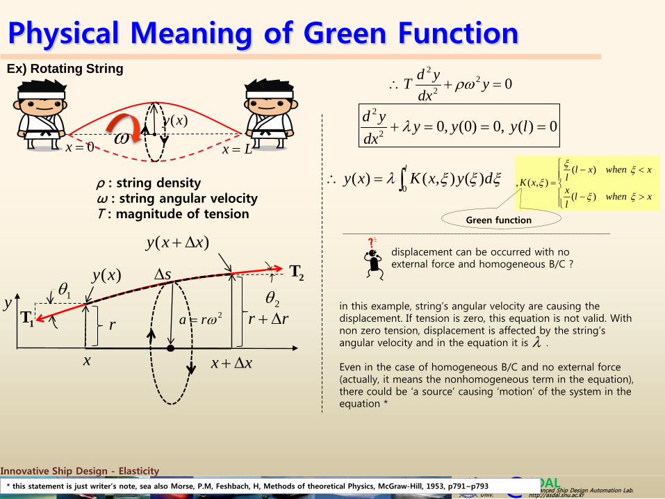
Physical Meaning of Green Function
)(xy
Lx =0=x ω
Ex) Rotating String
1θ
1T
2T
2θ
xx ∆+x
y( )y x
( )y x x+ ∆
r
ρ : string density ω : string angular velocityT : magnitude of tension
r r+ ∆
s∆
2ωra =
022
2
=+∴ ydx
ydT ρω
displacement can be occurred with no external force and homogeneous B/C ?
2
2 0, (0) 0, ( ) 0d y y y y ldx
λ+ = = =
0( ) ( , ) ( )
ly x K x y dλ ξ ξ ξ∴ = ∫
( ), ( , )
( )
l x when xlK xx l when xl
ξ ξξ
ξ ξ
− <= − >
Green function
in this example, string’s angular velocity are causing the displacement. If tension is zero, this equation is not valid. With non zero tension, displacement is affected by the string’s angular velocity and in the equation it is .
Even in the case of homogeneous B/C and no external force (actually, it means the nonhomogeneous term in the equation), there could be ‘a source’ causing ‘motion’ of the system in the equation *
λ
* this statement is just writer’s note, sea also Morse, P.M, Feshbach, H, Methods of theoretical Physics, McGraw-Hill, 1953, p791~p793

Innovative Ship Design - ElasticitySDAL@Advanced Ship Design Automation Lab.http://asdal.snu.ac.kr
Seoul NationalUniv.
Relation between differential and integral equations
Example : Boundary Value Problem
2
2 0, (0) 0, ( ) 0d y y y y ldx
λ+ = = =
0( ) ( , ) ( )
ly x K x y dλ ξ ξ ξ∴ = ∫
( ), ( , )
( )
l x when xlK xx l when xl
ξ ξξ
ξ ξ
− <= − >
2
2
d y ydx
λ∴ = −
0
0
( ) ( ) ( ) ( ) ( ) ( ) ( )
( ) ( ) ( )
x l
x
x l
x
dy y d x l x y x l y d x l x y xdx l
y d l y dl
λ ξ ξ ξ ξ ξ ξ
λ ξ ξ ξ ξ ξ ξ
= − + − + − − −
= − + −
∫ ∫
∫ ∫
To recover differential equation from integral equation, differentiate
[ ]2
2 ( ) ( ) ( ) ( )d y x y x l x y x y xdx l
λ λ= − − − = −
0( ) ( ) ( ) ( ) ( )
x l
x
xy x l x y d l y dl lξλ ξ ξ λ ξ ξ ξ= − + −∫ ∫
0( ) ( ) ( ) ( )
x l
x
dy d d xl x y d l y ddx dx l dx l
ξλ ξ ξ λ ξ ξ ξ= − + −∫ ∫
( ) ( )
( ) ( )
( , )( , ) [ , ( )] [ , ( )]B x B x
A x A x
d F x dB dAF x d d F x B x F x A xdx x dx dx
ξξ ξ ξ∂= + −
∂∫ ∫by using

Innovative Ship Design - ElasticitySDAL@Advanced Ship Design Automation Lab.http://asdal.snu.ac.kr
Seoul NationalUniv.
Integral Equations : The green’s function

Innovative Ship Design - ElasticitySDAL@Advanced Ship Design Automation Lab.http://asdal.snu.ac.kr
Seoul NationalUniv.
The green’s functionLinear second order differential equation
2
2 ( ) ( ) ( )d y dyA x B x y f xdx dx
+ + =
0 0( ) , ( )y a y y a y′ ′= =Initial condition :
( ) ( , ) ( ) ( ),b
ay x K x y d F xξ ξ ξ= +∫Fredholm integral equation of second kind
,F K : given functions and continuous in (a,b)
: function is to be determined which is continuous in (a,b) ( )y x
consider this form
( ) 0y x+ Φ =L2
2, d d d dp dwhere p q p qdx dx dx dx dx
= + = + +
L
homogeneous boundary conditions
0dyydx
α β+ =
, ( ) ( , ( ))x x y xφΦ =
For some constant values of α and β, which are imposed at the end points of an interval a≤x≤b.
In order to obtain a convenient reformulation of this problem, we first attemptthe determination of a Green’s function G which, for a given number ξ,
which has the four following properties.
1
2
( )( )
G x when xG
G x when xξξ
<= >
1. The function G1 and G2 satisfy the equation LG=0 in their intervals of definition; that is, LG1=0 when x<ξ , and LG2=0 when x>ξ.
2. The function G satisfies the homogeneous conditions prescribed at the end points x=a and x=b; that is, G1 satisfies the condition prescribed at x=a, and G2that corresponding to x=b.
3. The function G is continuous at x=ξ; that is, G1(ξ)=G2(ξ)
4. The derivative of G has a discontinuity of magnitude -1/p(ξ) at the point x=ξ; that is, 2 1( ) ( ) 1/ ( )G G pξ ξ ξ′ ′− = −
( ) ( , ) ( )b
ay x G x dξ ξ ξ= Φ∫
When the function exists, the original formulation of the problem can be transformed to the relation( , )G x ξ
solution : ( )integral equation : ( , )
if xif x yΦ = Φ
Φ = Φthen, how to get G?
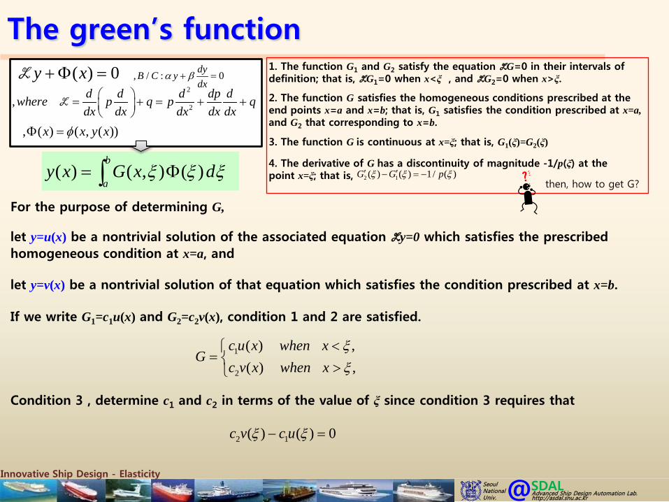
Innovative Ship Design - ElasticitySDAL@Advanced Ship Design Automation Lab.http://asdal.snu.ac.kr
Seoul NationalUniv.
The green’s function
1
2
( ) ,( ) ,
c u x when xG
c v x when xξξ
<= >
let y=u(x) be a nontrivial solution of the associated equation Ly=0 which satisfies the prescribed homogeneous condition at x=a, and
let y=v(x) be a nontrivial solution of that equation which satisfies the condition prescribed at x=b.
If we write G1=c1u(x) and G2=c2v(x), condition 1 and 2 are satisfied.
Condition 3 , determine c1 and c2 in terms of the value of ξ since condition 3 requires that
2 1( ) ( ) 0c v c uξ ξ− =
For the purpose of determining G,
1. The function G1 and G2 satisfy the equation LG=0 in their intervals of definition; that is, LG1=0 when x<ξ , and LG2=0 when x>ξ.
2. The function G satisfies the homogeneous conditions prescribed at the end points x=a and x=b; that is, G1 satisfies the condition prescribed at x=a,and G2 that corresponding to x=b.
3. The function G is continuous at x=ξ; that is, G1(ξ)=G2(ξ)
4. The derivative of G has a discontinuity of magnitude -1/p(ξ) at the point x=ξ; that is,
then, how to get G?
( ) 0y x+ Φ =L2
2, d d d dp dwhere p q p qdx dx dx dx dx
= + = + +
L
, / : 0dyB C ydx
α β+ =
, ( ) ( , ( ))x x y xφΦ =
( ) ( , ) ( )b
ay x G x dξ ξ ξ= Φ∫ 2 1( ) ( ) 1/ ( )G G pξ ξ ξ′ ′− = −

Innovative Ship Design - ElasticitySDAL@Advanced Ship Design Automation Lab.http://asdal.snu.ac.kr
Seoul NationalUniv.
The green’s function
2 11( ) ( ) ( )( )
c v c u bp
ξ ξξ
′ ′− = −
1
2
( ) ,( ) ,
c u x when xG
c v x when xξξ
<= >
2 1( ) ( ) 0 ( )c v c u aξ ξ− =
from condition 1, 2 :
from condition 3 :
for condition 4 :
1
2
0( ) ( )
1( ) ( )
( )
cu vcu v
p
ξ ξξ ξ
ξ
− = −′ ′−
We can get the value of as 1 2,c c 1
2
0( ) ( )1
1( ) ( )( ) ( ) ( ) ( )
( )
c v vc u uu v u v
p
ξ ξξ ξξ ξ ξ ξ
ξ
′ − = −′′ ′ −− +
only when ( ) ( ) ( ) ( ) 0u v u vξ ξ ξ ξ′ ′− + ≠ means the functions u and v are linearly independent
how to get G when they are linearly dependent?*
* Hildebrand, F.B., Methods of Applied Mathematics, Second edition, Dover, 1985, p300
1. The function G1 and G2 satisfy the equation LG=0 in their intervals of definition; that is, LG1=0 when x<ξ , and LG2=0 when x>ξ.
2. The function G satisfies the homogeneous conditions prescribed at the end points x=a and x=b; that is, G1 satisfies the condition prescribed at x=a,and G2 that corresponding to x=b.
3. The function G is continuous at x=ξ; that is, G1(ξ)=G2(ξ)
4. The derivative of G has a discontinuity of magnitude -1/p(ξ) at the point x=ξ; that is, 2 1( ) ( ) 1/ ( )G G pξ ξ ξ′ ′− = −
then, how to get G?
( ) 0y x+ Φ =L2
2, d d d dp dwhere p q p qdx dx dx dx dx
= + = + +
L
, / : 0dyB C ydx
α β+ =
, ( ) ( , ( ))x x y xφΦ =
( ) ( , ) ( )b
ay x G x dξ ξ ξ= Φ∫

Innovative Ship Design - ElasticitySDAL@Advanced Ship Design Automation Lab.http://asdal.snu.ac.kr
Seoul NationalUniv.
The green’s function
2 11( ) ( ) ( )( )
c v c u bp
ξ ξξ
′ ′− = −
1
2
( ) ,( ) ,
c u x when xG
c v x when xξξ
<= >
2 1( ) ( ) 0 ( )c v c u aξ ξ− =
from condition 1, 2 :
from condition 3 :
for condition 4 :
1
2
0( ) ( )
1( ) ( )
( )
cu vcu v
p
ξ ξξ ξ
ξ
− = −′ ′−
We can get the value of as 1 2,c c 1
2
0( ) ( )1
1( ) ( )( ) ( ) ( ) ( )
( )
c v vc u uu v u v
p
ξ ξξ ξξ ξ ξ ξ
ξ
′ − = −′′ ′ −− + only when ( ) ( ) ( ) ( ) 0u v u vξ ξ ξ ξ′ ′− ≠ means the functions u and v are linearly independent
1. The function G1 and G2 satisfy the equation LG=0 in their intervals of definition; that is, LG1=0 when x<ξ , and LG2=0 when x>ξ.
2. The function G satisfies the homogeneous conditions prescribed at the end points x=a and x=b; that is, G1 satisfies the condition prescribed at x=a,and G2 that corresponding to x=b.
3. The function G is continuous at x=ξ; that is, G1(ξ)=G2(ξ)
4. The derivative of G has a discontinuity of magnitude -1/p(ξ) at the point x=ξ; that is, 2 1( ) ( ) 1/ ( )G G pξ ξ ξ′ ′− = −
then, how to get G?
( ) 0y x+ Φ =L2
2, d d d dp dwhere p q p qdx dx dx dx dx
= + = + +
L
, / : 0dyB C ydx
α β+ =
, ( ) ( , ( ))x x y xφΦ =
( ) ( , ) ( )b
ay x G x dξ ξ ξ= Φ∫
by the condition 1, 1 1 1
2 2 2
( ) 0 ( ) 0( ) 0 ( ) 0
G pc u qc u pu quG pc v qc v pv qv
at x ξ
′ ′ ′ ′= + = → + =′ ′ ′ ′= + = → + =
=
LL

Innovative Ship Design - ElasticitySDAL@Advanced Ship Design Automation Lab.http://asdal.snu.ac.kr
Seoul NationalUniv.
The green’s function
* Hildebrand, F.B., Methods of Applied Mathematics, Second edition, Dover, 1985, p300
by the condition 1, 1 1 1
2 2 2
( ) 0 ( ) 0( ) 0 ( ) 0
G pc u qc u pu quG pc v qc v pv qv
at x ξ
′ ′ ′ ′= + = → + =′ ′ ′ ′= + = → + =
=
LL
( ) 0 ( )( ) 0 ( )pu qu apv qv b
′ ′ + =′ ′ + =
( ) : ( ) 0( ) : ( ) 0
v a v pu v quu b u pv u qv
′ ′⋅ + =′ ′⋅ + =
[ ]
[ ]
( ) ( ) :( ) ( ) 0
0( ) ( ) 0( ) ( ) 0( ) ( ') ( ) 0
( ) ' 0[ ( )] 0
u b v au pv v puu p v u p v v p u v pup u v u v p u v vup u v u v p u v vup u v u v p u v vu
p u v u v p u v vup uv
u
v
v v u
u
⋅ − ⋅′ ′ ′ ′− =
′ ′ ′′ ′ ′ ′′+ − − =′ ′ ′ ′′ ′′− + − =′ ′ ′ ′′ ′′− + − =′ ′ ′ ′ ′ ′− + − =
′′ ′ ′
′ ′ ′
′− + − =
′ ′
−
′−
′
=
+
( ) , :
( ) ( ) ( ) ( )( )
p uv vu A A constAu v v u
pξ ξ ξ ξ
ξ
′ ′∴ − =
′ ′∴ − =

Innovative Ship Design - ElasticitySDAL@Advanced Ship Design Automation Lab.http://asdal.snu.ac.kr
Seoul NationalUniv.
The green’s function
2 11( ) ( ) ( )( )
c v c u bp
ξ ξξ
′ ′− = −
1
2
( ) ,( ) ,
c u x when xG
c v x when xξξ
<= >
2 1( ) ( ) 0 ( )c v c u aξ ξ− =
from condition 1, 2 :
from condition 3 :
for condition 4 :
1
2
0( ) ( )
1( ) ( )
( )
cu vcu v
p
ξ ξξ ξ
ξ
− = −′ ′−
We can get the value of as 1 2,c c 1
2
0( ) ( )1
1( ) ( )( ) ( ) ( ) ( )
( )
c v vc u uu v u v
p
ξ ξξ ξξ ξ ξ ξ
ξ
′ − = −′′ ′ −− + only when ( ) ( ) ( ) ( ) 0u v u vξ ξ ξ ξ′ ′− ≠ means the functions u and v are linearly independent
* Hildebrand, F.B., Methods of Applied Mathematics, Second edition, Dover, 1985, p300
1. The function G1 and G2 satisfy the equation LG=0 in their intervals of definition; that is, LG1=0 when x<ξ , and LG2=0 when x>ξ.
2. The function G satisfies the homogeneous conditions prescribed at the end points x=a and x=b; that is, G1 satisfies the condition prescribed at x=a,and G2 that corresponding to x=b.
3. The function G is continuous at x=ξ; that is, G1(ξ)=G2(ξ)
4. The derivative of G has a discontinuity of magnitude -1/p(ξ) at the point x=ξ; that is, 2 1( ) ( ) 1/ ( )G G pξ ξ ξ′ ′− = −
then, how to get G?
( ) 0y x+ Φ =L2
2, d d d dp dwhere p q p qdx dx dx dx dx
= + = + +
L
, / : 0dyB C ydx
α β+ =
, ( ) ( , ( ))x x y xφΦ =
( ) ( , ) ( )b
ay x G x dξ ξ ξ= Φ∫
by the condition 1, 1 1 1
2 2 2
( ) 0 ( ) 0( ) 0 ( ) 0
G pc u qc u pu quG pc v qc v pv qv
at x ξ
′ ′ ′ ′= + = → + =′ ′ ′ ′= + = → + =
=
LL
( ) ( ) ( ) ( ) , :( )Au v v u A const
pξ ξ ξ ξ
ξ′ ′− =

Innovative Ship Design - ElasticitySDAL@Advanced Ship Design Automation Lab.http://asdal.snu.ac.kr
Seoul NationalUniv.
The green’s function
2 11( ) ( ) ( )( )
c v c u bp
ξ ξξ
′ ′− = −
1
2
( ) ,( ) ,
c u x when xG
c v x when xξξ
<= >
2 1( ) ( ) 0 ( )c v c u aξ ξ− =
from condition 1, 2 :
from condition 3 :
for condition 4 :
1
2
0( ) ( )
1( ) ( )
( )
cu vcu v
p
ξ ξξ ξ
ξ
− = −′ ′−
We can get the value of as 1 2,c c 1
2
0( ) ( )1
1( ) ( )( ) ( ) ( ) ( )
( )
c v vc u uu v u v
p
ξ ξξ ξξ ξ ξ ξ
ξ
′ − = −′′ ′ −− +
only when
* Hildebrand, F.B., Methods of Applied Mathematics, Second edition, Dover, 1985, p300
1. The function G1 and G2 satisfy the equation LG=0 in their intervals of definition; that is, LG1=0 when x<ξ , and LG2=0 when x>ξ.
2. The function G satisfies the homogeneous conditions prescribed at the end points x=a and x=b; that is, G1 satisfies the condition prescribed at x=a,and G2 that corresponding to x=b.
3. The function G is continuous at x=ξ; that is, G1(ξ)=G2(ξ)
4. The derivative of G has a discontinuity of magnitude -1/p(ξ) at the point x=ξ; that is, 2 1( ) ( ) 1/ ( )G G pξ ξ ξ′ ′− = −
then, how to get G?
( ) 0y x+ Φ =L2
2, d d d dp dwhere p q p qdx dx dx dx dx
= + = + +
L
, / : 0dyB C ydx
α β+ =
, ( ) ( , ( ))x x y xφΦ =
( ) ( , ) ( )b
ay x G x dξ ξ ξ= Φ∫
( ) ( ) ( ) ( ) 0u v u vξ ξ ξ ξ′ ′− ≠
( ) ( ) ( ) ( ) , :( )Au v v u A const
pξ ξ ξ ξ
ξ′ ′− =
1
2
( ) ( )0( ) ( ) ( )( ) ( )
1( ) ( ) ( ) ( )
( )( )
v vc v v pp p Ac u u u uA A
pp A
ξ ξξ ξ ξξ ξξ ξ ξ ξ
ξξ
− ′ − ∴ = − = − = −′ − −

Innovative Ship Design - ElasticitySDAL@Advanced Ship Design Automation Lab.http://asdal.snu.ac.kr
Seoul NationalUniv.
The green’s function
2 11( ) ( ) ( )( )
c v c u bp
ξ ξξ
′ ′− = −
1
2
( ) ,( ) ,
c u x when xG
c v x when xξξ
<= >
2 1( ) ( ) 0 ( )c v c u aξ ξ− =
from condition 1, 2 :
from condition 3 :
for condition 4 :
1
2
0( ) ( )
1( ) ( )
( )
cu vcu v
p
ξ ξξ ξ
ξ
− = −′ ′−
We can get the value of as 1 2,c c1
2
0( ) ( )1
1( ) ( )( ) ( ) ( ) ( )
( )
c v vc u uu v u v
p
ξ ξξ ξξ ξ ξ ξ
ξ
′ − = −′′ ′ −− +
only when
* Hildebrand, F.B., Methods of Applied Mathematics, Second edition, Dover, 1985, p300
1. The function G1 and G2 satisfy the equation LG=0 in their intervals of definition; that is, LG1=0 when x<ξ , and LG2=0 when x>ξ.
2. The function G satisfies the homogeneous conditions prescribed at the end points x=a and x=b; that is, G1 satisfies the condition prescribed at x=a,and G2 that corresponding to x=b.
3. The function G is continuous at x=ξ; that is, G1(ξ)=G2(ξ)
4. The derivative of G has a discontinuity of magnitude -1/p(ξ) at the point x=ξ; that is, 2 1( ) ( ) 1/ ( )G G pξ ξ ξ′ ′− = −
then, how to get G?
( ) 0y x+ Φ =L2
2, d d d dp dwhere p q p qdx dx dx dx dx
= + = + +
L
, / : 0dyB C ydx
α β+ =
, ( ) ( , ( ))x x y xφΦ =
( , )( ) ( )b
aGy xx dξ ξξ= Φ∫
( ) ( ) ( ) ( ) 0u v u vξ ξ ξ ξ′ ′− ≠
( ) ( ) ( ) ( ) , :( )Au v v u A const
pξ ξ ξ ξ
ξ′ ′− =
1
2
( )
( )
vc Ac u
A
ξ
ξ
− =
− 1 ( ) ( )
1 ( ) ( )( , )
u x v when xA
v x u whx
e xA
Gn
ξ ξ
ξ ξξ
− <∴ = − >
where A is a constant, independent of ,x ξ

Innovative Ship Design - ElasticitySDAL@Advanced Ship Design Automation Lab.http://asdal.snu.ac.kr
Seoul NationalUniv.
The green’s functionLinear second order differential equation
2
2 ( ) ( ) ( )d y dyA x B x y f xdx dx
+ + =
0 0( ) , ( )y a y y a y′ ′= =Initial condition :
( ) ( , ) ( ) ( ),b
ay x K x y d F xξ ξ ξ= +∫Fredholm integral equation of second kind
,F K : given functions and continuous in (a,b)
: function is to be determined which is continuous in (a,b) ( )y x
consider this form
( ) 0y x+ Φ =L2
2, d d d dp dwhere p q p qdx dx dx dx dx
= + = + +
L
homogeneous boundary conditions
0dyydx
α β+ =
, ( ) ( , ( ))x x y xφΦ =
For some constant values of α and β, which are imposed at the end points of an interval a≤x≤b. 1. The function G1 and G2 satisfy the equation LG=0 in their intervals of
definition; that is, LG1=0 when x<ξ , and LG2=0 when x>ξ.
2. The function G satisfies the homogeneous conditions prescribed at the end points x=a and x=b; that is, G1 satisfies the condition prescribed at x=a, and G2that corresponding to x=b.
3. The function G is continuous at x=ξ; that is, G1(ξ)=G2(ξ)
4. The derivative of G has a discontinuity of magnitude -1/p(ξ) at the point x=ξ; that is, 2 1( ) ( ) 1/ ( )G G pξ ξ ξ′ ′− = −
( , )( ) ( )b
aGy xx dξ ξξ= Φ∫
When the function exists, the original formulation of the problem can be transformed to the relation
( , )G x ξ
solution : ( )integral equation : ( , )
if xif x yΦ = Φ
Φ = Φ
1( ) ( ) ( ) ( ) ( ) ( ) ( )x b
a xy x u v x d u x v d
Aξ ξ ξ ξ ξ ξ = − Φ + Φ ∫ ∫
1 ( ) ( )
1 ( ) ( )( , )
u x v when xA
v x u whx
e xA
Gn
ξ ξ
ξ ξξ
− <∴ = − >
in explicit form

Innovative Ship Design - ElasticitySDAL@Advanced Ship Design Automation Lab.http://asdal.snu.ac.kr
Seoul NationalUniv.
The green’s functionLinear second order differential equation
( ) 0y x+ Φ =L
2
2
d d d dp dp q p qdx dx dx dx dx
= + = + +
L
0dyydx
α β+ =
, ( ) ( , ( ))x x y xφΦ =( , )( ) ( )
b
aGy xx dξ ξξ= Φ∫
When the function exists, the original formulation of the problem can be transformed to the relation
( , )G x ξ
solution : ( )integral equation : ( , )
if xif x yΦ = Φ
Φ = Φ
1( ) ( ) ( ) ( ) ( ) ( ) ( )x b
a xy x u v x d u x v d
Aξ ξ ξ ξ ξ ξ = − Φ + Φ ∫ ∫
1 ( ) ( )
1 ( ) ( ), ( , )
u x v whenG x
xA
v x u when xA
ξ ξ
ξ ξξ
− <= − >
homogeneous B/C
[ ]( ) ( ) ( ) ( ) ( )A p u v v uξ ξ ξ ξ ξ′ ′= −
( ) ( , ) ( )b
ay x G x dξ ξ ξ= Φ∫
( ) 0y x+ Φ =Limplies the differential equation
Show that
( ) ( )
( ) ( )
( , )( , ) [ , ( )] [ , ( )]B x B x
A x A x
d F x dB dAF x d d F x B x F x A xdx x dx dx
ξξ ξ ξ∂= + −
∂∫ ∫differentiate by using
1( ) ( ) ( ) ( ) ( ) ( ) ( )x b
a xy x v x u d u x v d
Aξ ξ ξ ξ ξ ξ ′ ′ ′= − Φ + Φ ∫ ∫
1 1( ) ( ) ( ) ( ) ( ) ( ) ( ) [ ( ) ( ) ( ) ( )] ( )x b
a xy x v x u d u x v d v x u x u x v x x
A Aξ ξ ξ ξ ξ ξ ′′ ′′ ′′ ′ ′= − Φ + Φ − − Φ ∫ ∫
1 ( )( ) ( ) ( ) ( ) ( ) ( ) ( ) ( ) ( ) ( ) [ ( ) ( ) ( ) ( )] ( )x b
a x
p xp x y x p x v x u d p x u x v d v x u x u x v x xA A
ξ ξ ξ ξ ξ ξ ′′ ′′ ′′ ′ ′= − Φ + Φ − − Φ ∫ ∫
1( ) ( ) ( ) ( ) ( ) ( ) ( ) ( ) ( ) ( )x b
a xp x y x p x v x u d p x u x v d
Aξ ξ ξ ξ ξ ξ ′ ′ ′ ′ ′ ′= − Φ + Φ ∫ ∫

Innovative Ship Design - ElasticitySDAL@Advanced Ship Design Automation Lab.http://asdal.snu.ac.kr
Seoul NationalUniv.
( ) ( , ) ( ) ( ) ( , ) ( ) (4 0 )b b
a ay x G x r y d G x f dλ ξ ξ ξ ξ ξ ξ ξ= −∫ ∫
The green’s functionLinear second order differential equation
( ) 0y x+ Φ =L
2
2
d d d dp dp q p qdx dx dx dx dx
= + = + +
L
0dyydx
α β+ =
, ( ) ( , ( ))x x y xφΦ =( , )( ) ( )
b
aGy xx dξ ξξ= Φ∫
When the function exists, the original formulation of the problem can be transformed to the relation
( , )G x ξ
solution : ( )integral equation : ( , )
if xif x yΦ = Φ
Φ = Φ
1( ) ( ) ( ) ( ) ( ) ( ) ( )x b
a xy x u v x d u x v d
Aξ ξ ξ ξ ξ ξ = − Φ + Φ ∫ ∫
1 ( ) ( )
1 ( ) ( ), ( , )
u x v whenG x
xA
v x u when xA
ξ ξ
ξ ξξ
− <= − >
homogeneous B/C
[ ]( ) ( ) ( ) ( ) ( )A p u v v uξ ξ ξ ξ ξ′ ′= −
( ) ( ) ( ) ( )y x r x y x f xλ+ =LIn particular, ( ) ( ) ( ) ( )x r x y x f xλΦ = −
where G is relevant Green’s function.
( ) ( ) ( )r x y x Y x=
( )( ) ( , ) ( ) ( , )( )
b b
a a
fY x K x Y d K x drξλ ξ ξ ξ ξ ξξ
= −∫ ∫
Kernel is actually the product , and is not symmetric unless r(x) is a constant. However if we write
( , ) ( )G x rξ ξ( , )K x ξ
Under the assumption that r(x) is nonnegative over (a,b), the equation can be written in the form
( , ) ( ) ( ) ( , )K x r x r G xξ ξ ξ=Where is defined by the relationK
Hence possesses the same symmetry as G. ( )( , ) ( , )K x K xξ ξ=

Innovative Ship Design - ElasticitySDAL@Advanced Ship Design Automation Lab.http://asdal.snu.ac.kr
Seoul NationalUniv.
( ) ( , ) ( ) ( ) ( , ) ( ) (4 0 )b b
a ay x G x r y d G x f dλ ξ ξ ξ ξ ξ ξ ξ= −∫ ∫
The green’s functionLinear second order differential equation
( ) 0y x+ Φ =L
2
2
d d d dp dp q p qdx dx dx dx dx
= + = + +
L
0dyydx
α β+ =
, ( ) ( , ( ))x x y xφΦ =( , )( ) ( )
b
aGy xx dξ ξξ= Φ∫
When the function exists, the original formulation of the problem can be transformed to the relation
( , )G x ξ
solution : ( )integral equation : ( , )
if xif x yΦ = Φ
Φ = Φ
1( ) ( ) ( ) ( ) ( ) ( ) ( )x b
a xy x u v x d u x v d
Aξ ξ ξ ξ ξ ξ = − Φ + Φ ∫ ∫
1 ( ) ( )
1 ( ) ( ), ( , )
u x v whenG x
xA
v x u when xA
ξ ξ
ξ ξξ
− <= − >
homogeneous B/C
[ ]( ) ( ) ( ) ( ) ( )A p u v v uξ ξ ξ ξ ξ′ ′= −
( ) ( ) ( ) ( )y x r x y x f xλ+ =LIn particular, ( ) ( ) ( ) ( )x r x y x f xλΦ = −
where G is relevant Green’s function.
In the special case when the operator L and the associated end conditions are such that
, (0 ) ( ) 0y y y y l′′≡ = =L ( ) ( ),( , )
( ) ( ).
x l xlG x
l x xl
ξ ξξ
ξ ξ
− <= − >
it is readily verified that the relevant Green’s function G is identified with the kernel K defined by
Thus, in particular, the solution of the problem
( ), (0) ( ) 0y f xy y l′′ =
= = 0( ) ( , ) ( ) ,
ly x G x f dξ ξ ξ= −∫
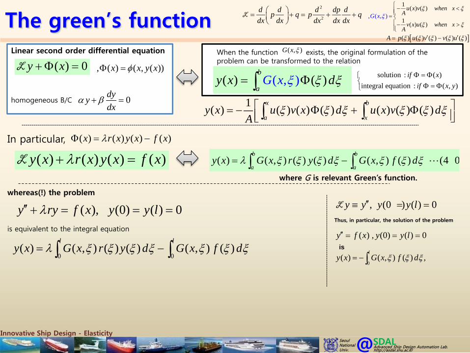
Innovative Ship Design - ElasticitySDAL@Advanced Ship Design Automation Lab.http://asdal.snu.ac.kr
Seoul NationalUniv.
( ) ( , ) ( ) ( ) ( , ) ( ) (4 0 )b b
a ay x G x r y d G x f dλ ξ ξ ξ ξ ξ ξ ξ= −∫ ∫
The green’s functionLinear second order differential equation
( ) 0y x+ Φ =L
2
2
d d d dp dp q p qdx dx dx dx dx
= + = + +
L
0dyydx
α β+ =
, ( ) ( , ( ))x x y xφΦ =( , )( ) ( )
b
aGy xx dξ ξξ= Φ∫
When the function exists, the original formulation of the problem can be transformed to the relation
( , )G x ξ
solution : ( )integral equation : ( , )
if xif x yΦ = Φ
Φ = Φ
1( ) ( ) ( ) ( ) ( ) ( ) ( )x b
a xy x u v x d u x v d
Aξ ξ ξ ξ ξ ξ = − Φ + Φ ∫ ∫
1 ( ) ( )
1 ( ) ( ), ( , )
u x v whenG x
xA
v x u when xA
ξ ξ
ξ ξξ
− <= − >
homogeneous B/C
[ ]( ) ( ) ( ) ( ) ( )A p u v v uξ ξ ξ ξ ξ′ ′= −
( ) ( ) ( ) ( )y x r x y x f xλ+ =LIn particular, ( ) ( ) ( ) ( )x r x y x f xλΦ = −
where G is relevant Green’s function.
, (0 ) ( ) 0y y y y l′′≡ = =LThus, in particular, the solution of the problem
( ) , (0) ( ) 0y f x y y l′′ = = =
0( ) ( , ) ( ) ,
ly x G x f dξ ξ ξ= −∫is
whereas(!) the problem
( ), (0) ( ) 0y ry f x y y lλ′′ + = = =is equivalent to the integral equation
0 0( ) ( , ) ( ) ( ) ( , ) ( )
l ly x G x r y d G x f dλ ξ ξ ξ ξ ξ ξ ξ= −∫ ∫

Innovative Ship Design - ElasticitySDAL@Advanced Ship Design Automation Lab.http://asdal.snu.ac.kr
Seoul NationalUniv.
The green’s function
When the prescribed end condition are not homogeneous, a modified procedure is needed.
In this case, we denote by G(x,ξ) the Green’s function corresponding the associated homogeneous end conditions, and attempt to determine a function P(x) such that the relation
( )( ) ( ), ( ) ( )y a f x y b g x= =
The requirement imply
( ) 0P x =L
( ) ( , ) ( ) ( ) ( , ) ( ) (4 0 )b b
a ay x G x r y d G x f dλ ξ ξ ξ ξ ξ ξ ξ= −∫ ∫ ( ) ( ) ( ) ( )y x r x y x f xλ+ =L
In particular, ( ) ( ) ( ) ( )x r x y x f xλΦ = −
where G is relevant Green’s function.
( ) 0y x+ Φ =L ( ) ( , ) ( )b
ay x G x dξ ξ ξ= Φ∫
2
2
d d d dp dp q p qdx dx dx dx dx
= + = + +
L
0dyydx
α β+ =homogeneous B/C
( )( ) ( , ) ( ) ( ) 0b
aP x G x d xξ ξ ξ+ Φ +Φ =∫L
( ) ( , ) ( ) ( ) 0b
aP x G x d xξ ξ ξ+ Φ +Φ =∫L L
zero with homogeneous end condition
nonhomogeneous end condition
( ) ( ) ( , ) ( )b
ay x P x G x dξ ξ ξ= + Φ∫
( ) ( ) 0y x x+Φ =Lis equivalent to the differential equation
together with the prescribed nonhomogeneous end conditions.

Innovative Ship Design - ElasticitySDAL@Advanced Ship Design Automation Lab.http://asdal.snu.ac.kr
Seoul NationalUniv.
The green’s function
( ) 0P x =L
( ) ( , ) ( ) ( ) ( , ) ( ) (4 0 )b b
a ay x G x r y d G x f dλ ξ ξ ξ ξ ξ ξ ξ= −∫ ∫ ( ) ( ) ( ) ( )y x r x y x f xλ+ =L
In particular, ( ) ( ) ( ) ( )x r x y x f xλΦ = −
where G is relevant Green’s function.
( ) 0y x+ Φ =L ( ) ( , ) ( )b
ay x G x dξ ξ ξ= Φ∫
2
2
d d d dp dp q p qdx dx dx dx dx
= + = + +
L
0dyydx
α β+ =homogeneous B/C
( ) ( , ) ( ) ( ) 0b
aP x G x d xξ ξ ξ+ Φ +Φ =∫L L
zero with homogeneous end condition
nonhomogeneous end condition
( ) ( ) ( , ) ( )b
ay x P x G x dξ ξ ξ= + Φ∫
1, (0) 0, ( ) 1y xy y y l′′ + = = =
(0 )0, ( ) 0y y l= =
( ) 0, (0) 0, ( ) 1,P x P P l′′ = = =
( ) ( ) 1,x xy xΦ = −
example)
attempt to determine,
with Green function to the homogeneous end conditions
and satisfying the nonhomogeneous end conditions ( )P x
in the problem, y y′′≡L
( ) 0y x∴ +Φ =L
( ) ( ), ( , )
( ) ( )
l x xlG xx l xl
ξ ξξ
ξ ξ
− <= − >

Innovative Ship Design - ElasticitySDAL@Advanced Ship Design Automation Lab.http://asdal.snu.ac.kr
Seoul NationalUniv.
The green’s function
( ) ( , ) ( ) ( ) ( , ) ( ) (4 0 )b b
a ay x G x r y d G x f dλ ξ ξ ξ ξ ξ ξ ξ= −∫ ∫ ( ) ( ) ( ) ( )y x r x y x f xλ+ =L
In particular, ( ) ( ) ( ) ( )x r x y x f xλΦ = −
where G is relevant Green’s function.
( ) 0y x+ Φ =L ( ) ( , ) ( )b
ay x G x dξ ξ ξ= Φ∫
2
2
d d d dp dp q p qdx dx dx dx dx
= + = + +
L
0dyydx
α β+ =homogeneous B/C
( ) ( ) ( , ) ( )b
ay x P x G x dξ ξ ξ= + Φ∫
1, (0) 0, ( ) 1y xy y y l′′ + = = =
(0 )0, ( ) 0y y l= =
( ) 0, (0) 0, ( ) 1,P x P P l′′ = = =
( ) xP xl
∴ =by the B/C
example)
attempt to determine,
with Green function to the homogeneous end conditions
and satisfying the nonhomogeneous end conditions ( )P x
( ) ( ) 1,x xy xΦ = − y y′′≡Lin the problem,
1
1 2
( )( )
P x cP x c x c′ =
= +
2
1
01
c
cl
=
=
( ) ( ), ( , )
( ) ( )
l x xlG xx l xl
ξ ξξ
ξ ξ
− <= − >

Innovative Ship Design - ElasticitySDAL@Advanced Ship Design Automation Lab.http://asdal.snu.ac.kr
Seoul NationalUniv.
The green’s function
( ) ( , ) ( ) ( ) ( , ) ( ) (4 0 )b b
a ay x G x r y d G x f dλ ξ ξ ξ ξ ξ ξ ξ= −∫ ∫ ( ) ( ) ( ) ( )y x r x y x f xλ+ =L
In particular, ( ) ( ) ( ) ( )x r x y x f xλΦ = −
where G is relevant Green’s function.
( ) 0y x+ Φ =L ( ) ( , ) ( )b
ay x G x dξ ξ ξ= Φ∫
2
2
d d d dp dp q p qdx dx dx dx dx
= + = + +
L
0dyydx
α β+ =homogeneous B/C
( ) ( ) ( , ) ( )b
ay x P x G x dξ ξ ξ= + Φ∫
1, (0) 0, ( ) 1y xy y y l′′ + = = =
0( ) ( , )[ ( ) 1]
lxy x G x y dl
ξ ξ ξ ξ∴ = + −∫
( ) ( ), ( , )
( ) ( )
l x xlwhere G xx l xl
ξ ξξ
ξ ξ
− <= − >
( ) xP xl
=
and reduces to the form
0( ) ( ) ( , ) ( )
2lx xy x l x G x y d
lξ ξ ξ ξ= − − + ∫
example)
attempt to determine,
( ) ( ) 1,x xy xΦ = −
0 0
22
02
2 2
3 32
2
( , ) ( ) ( )
1 1( ) ( )2 2
1 1 1( ) ( ) ( )2 2 21 1 1 12 2 2 21 12 21 ( )2
l x l
x
x l
x
xG x d l x d l dl l
xl x ll l
x x xl x l l l xl l l
x xx x xl xl l
x xl
x x l
ξξ ξ ξ ξ ξ
ξ ξ
− = − − − −
= − − − −
= − − − − + −
= − + − + + −
= − +
= − −
∫ ∫ ∫