Innovative SETI by the KLT

PoS(Dynamic2007)034

Copyright owned by the author(s) under the terms of the Creative Commons Attribution-NonCommercial-ShareAlike Licence. http://pos.sissa.it

Innovative SETI by the KLT

Claudio Maccone1 Co-Vice Chair, SETI Permanent Study Group, International Academy of Astronautics (IAA) Home address: Via Martorelli 43, I-10155 Torino (Turin), Italy E-mail: [email protected]

SETI searches are, by definition, the extraction of very weak radio signals out of the cosmic background noise. When SETI was born in 1959, it was “natural” to attempt this extraction by the only detection algorithm well known at the time: the Fourier Transform (FT). In fact: 1) SETI radio astronomers had adopted the viewpoint that a candidate ET signal would

necessarily be a sinusoidal carrier, i.e. a very narrow-band signal. Over such a narrow band, the background noise is necessarily white. And so, the basic assumption behind the FT that the background noise must be white was “perfectly matched” to SETI for the next fifty years!

2) In addition, the Americans, J. W. Cooley and J. W. Tukey discovered in April 1965 that all the FT computations could be speeded up to N*ln(N) (rather than N2) (N is the number of numbers to be processed) by their own Fast Fourier Transform (FFT). Then, SETI radio astronomers all over the world gladly and unquestioningly adopted the new FFT forever.

In 1983, however, the French SETI radio astronomer, François Biraud, dared to challenge this view (ref. [6]). He argued that we only can make guesses about ET’s telecommunication systems, and that the shifting trend on Earth was from narrow-band to wide-band telecommunications. Thus, a new transform, other than the FFT, was needed that could detect signals over both narrow and wide bands, regardless of the colored noise distribution over any finite bandwidth. Such a transform had actually been pointed out as early as 1946 by the Finn mathematician, Kari Karhunen, and the French mathematician, Michel Loève, and is thus named KLT for them. In conclusion, François Biraud suggested to “look for the unknown in SETI” by adopting the KLT rather than the FFT. The same ideas were reached independently by this author also, and starting 1987, he too was “preaching the KLT”: first at the SETI Institute, then (since 1990) at the Italian CNR (now called INAF) SETI facilities at Medicina, near Bologna. Their director, Stelio Montebugnoli, was willing to pay attention to him. Little by little, bright students succeeded in programming the KLT algorithm for the Medicina radio telescopes. Finally, by the year 2000, the advent of programmable cards, mastered by Montebugnoli, made the “miracle” happen. The KLT for SETI is now a reality at the SETI-Italia facilities and for the first time in history. This paper describes the KLT with a final section devoted to the advantages of installing the KLT on LOFAR and the SKA, i.e. to detecting leakage from nearby stars.

Bursts, Pulses and Flickering: Wide-field monitoring of the dynamic radio sky Kerastari, Tripolis, Greece 12-15 June, 2007

1 Speaker

PoS(Dynamic2007)034

Innovative SETI by the KLT Claudio Maccone

2

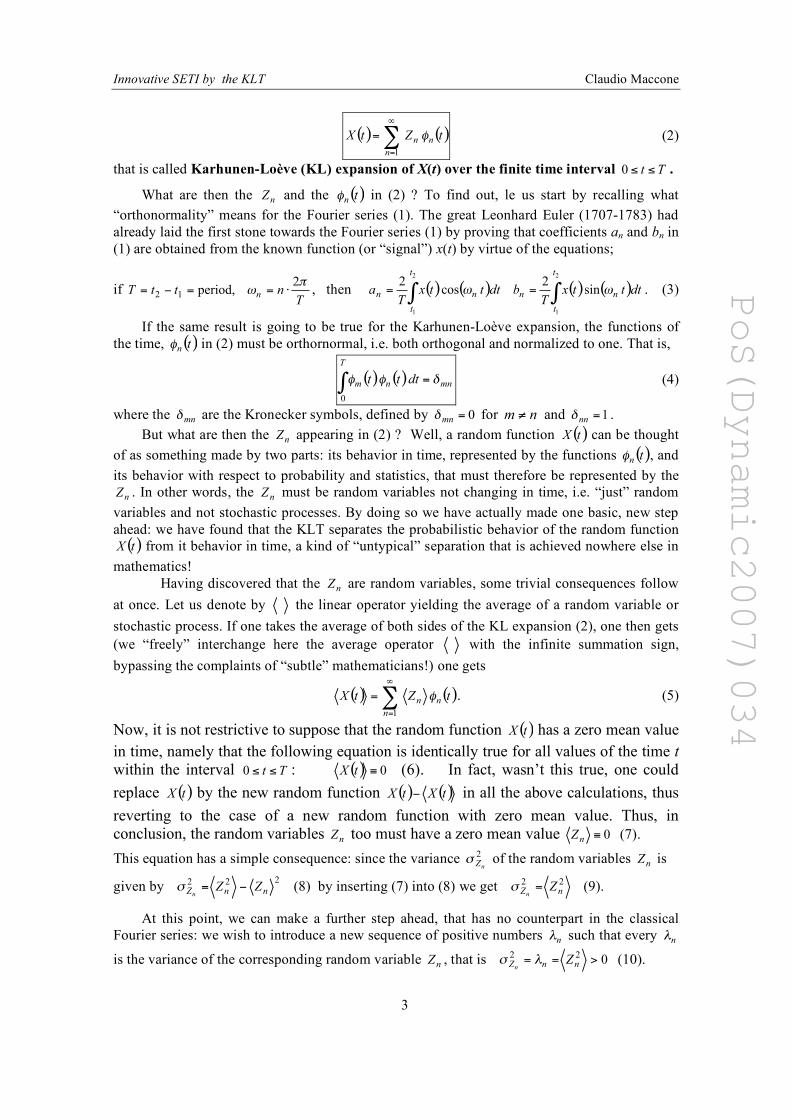
1. Introduction

The Karhunen-Loève Transform (KLT) is the most advanced mathematical algorithm available in the year 2007 to achieve both noise filtering and data compression in processing signals of any kind. It took about two centuries (~ 1800÷2000) to mathematicians to create such a jewel of thought little by little, piece after piece, paper after paper. It is thus difficult to recognize who did what in building up the KLT, and to be fair to each contributing author. In addition, mathematicians, both pure and applied, often speak such a “clumsy” language of their own that even learned scientists find sometimes hard to understand them. This unfortunate situation hides the aesthetic beauty of many mathematical discoveries that were often historically made by their authors more for the joy of opening new lines of thought than for the sake of any immediate application to science and engineering. In essence, the KLT is a rather new mathematical tool to improve our understanding of physical phoenomena, far superior to the classical Fourier Transform (FT). The KLT is named for two mathematicians, the (living) Finn, Kari Karhunen (ref. [1]) and the French-American, Michel Loève (1907-1979) (refs. [2] and [3]), who proved, independently and about the same time (1946), that the series (2) hereafter is convergent. Put this way, the KLT looks like a purely mathematical topic, but really this is hardly the case. As early as 1933 had the American statistician and economist Harold Hotelling (1895-1973) used the KLT (for discrete time, rather than for continuous time), so that the KLT is sometimes called the “Hotelling Transform”. Even much earlier than these three authors had the Italian geometer Eugenio Beltrami (1835-1899) discovered as early as 1873 the SVD (Singular Value Decomposition), that is closely related to the KLT in that area of applied mathematics nowadays called Principal Components Analysis (PCA). Unfortunately, a complete historical account about how these contributions developed since 1865 (when the English mathematician Arthur Cayley (1821-1895) “invented” matrices) simply does not exist. We only know about “fragments of thought” that impair an overall vision of both the PCA and the KLT. In the first three sections of this paper, we’ll derive heuristically and step-by-step the many equations that make up for the KLT. We think that this approach is much easier to understand for beginners than what is found in most “pure” mathematical textbooks, and hope that the readers will appreciate our effort to explain the KLT as easily as possible to non-mathematically trained people.

2. A heuristic derivation of the Karhunen-Loève (KL) Expansion

We start by saying that the KLT was born during the years of World War Two out of the need to merge two different areas of classical mathematics: 1) The expansion of a deterministic periodic signal ( )tx unto a basis of orthonormal functions

(sines and cosines, in this case), typified by the classical Fourier series (firstly put forward by the French mathematician Jean Baptiste Joseph Fourier (1768-1830) around 1807),

( ) ( ) ( )[ ]!"

=

++=

1

0sincos

2n

nnnntbta

atx ## . (1)

2) The need to extend to probability and statistics this too narrow and deterministic view. The much larger variety of phenomena called “noise” by physicists and engineers will thus be encompassed by the new transform. This enlarged view means to consider a random function ( )tX (notice that we denote random quantities by capitals, and that ( )tX is also called a

“stochastic process of the time”). We now seek to expand this stochastic process onto a set of orthonormal functions ( )t

n! according to the starting formula

PoS(Dynamic2007)034


3

( ) ( )!"

=

=

1

n

nntZtX # (2)

that is called Karhunen-Loève (KL) expansion of X(t) over the finite time interval Tt !!0 .

What are then the nZ and the ( )t

n! in (2) ? To find out, le us start by recalling what

“orthonormality” means for the Fourier series (1). The great Leonhard Euler (1707-1783) had already laid the first stone towards the Fourier series (1) by proving that coefficients an and bn in (1) are obtained from the known function (or “signal”) x(t) by virtue of the equations;

if T

nttTn

!"

2period,12 #==$= , then ( ) ( ) ( ) ( )dtttx

Tbdtttx

Ta

t

t

nn

t

t

nn !! ==

2

1

2

1

sin2

cos2

"" . (3)

If the same result is going to be true for the Karhunen-Loève expansion, the functions of the time, ( )t

n! in (2) must be orthornormal, i.e. both orthogonal and normalized to one. That is,

( ) ( )mn

T

nmdttt !"" =#

0

(4)

where the mn

! are the Kronecker symbols, defined by 0=mn

! for nm ! and 1=nn

! . But what are then the

nZ appearing in (2) ? Well, a random function ( )tX can be thought

of as something made by two parts: its behavior in time, represented by the functions ( )tn! , and

its behavior with respect to probability and statistics, that must therefore be represented by the nZ . In other words, the

nZ must be random variables not changing in time, i.e. “just” random

variables and not stochastic processes. By doing so we have actually made one basic, new step ahead: we have found that the KLT separates the probabilistic behavior of the random function ( )tX from it behavior in time, a kind of “untypical” separation that is achieved nowhere else in

mathematics! Having discovered that the

nZ are random variables, some trivial consequences follow

at once. Let us denote by the linear operator yielding the average of a random variable or stochastic process. If one takes the average of both sides of the KL expansion (2), one then gets (we “freely” interchange here the average operator with the infinite summation sign, bypassing the complaints of “subtle” mathematicians!) one gets

( ) ( )!"

=

=

1

n

nntZtX # . (5)

Now, it is not restrictive to suppose that the random function ( )tX has a zero mean value in time, namely that the following equation is identically true for all values of the time t within the interval Tt !!0 : ( ) 0!tX (6). In fact, wasn’t this true, one could replace ( )tX by the new random function ( ) ( )tXtX ! in all the above calculations, thus reverting to the case of a new random function with zero mean value. Thus, in conclusion, the random variables

nZ too must have a zero mean value 0!

nZ (7).

This equation has a simple consequence: since the variance 2

nZ

! of the random variables nZ is

given by 222

nnZZZ

n

!=" (8) by inserting (7) into (8) we get 22

nZZ

n

=! (9).

At this point, we can make a further step ahead, that has no counterpart in the classical Fourier series: we wish to introduce a new sequence of positive numbers

n! such that every

n!

is the variance of the corresponding random variable nZ , that is 0

22>==

nnZZ

n

!" (10).

PoS(Dynamic2007)034


4

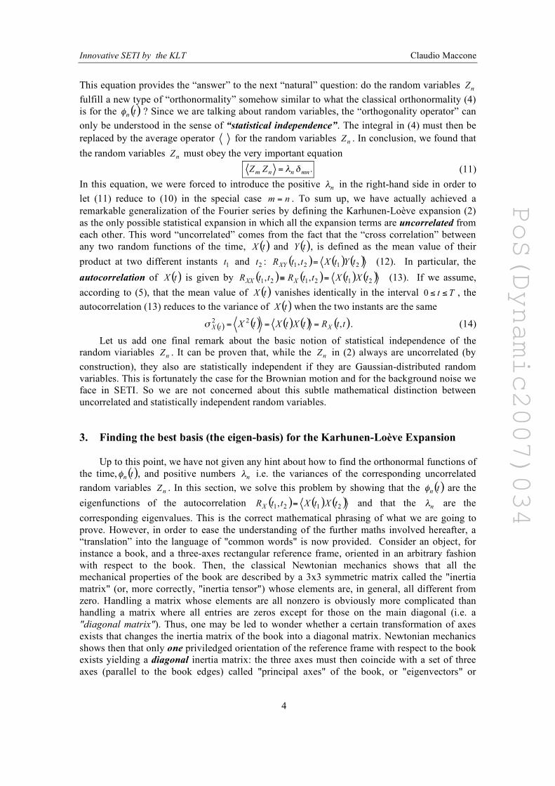
This equation provides the “answer” to the next “natural” question: do the random variables nZ

fulfill a new type of “orthonormality” somehow similar to what the classical orthonormality (4) is for the ( )t

n! ? Since we are talking about random variables, the “orthogonality operator” can

only be understood in the sense of “statistical independence”. The integral in (4) must then be replaced by the average operator for the random variables

nZ . In conclusion, we found that

the random variables nZ must obey the very important equation

.mnnnm

ZZ !"= (11) In this equation, we were forced to introduce the positive

n! in the right-hand side in order to

let (11) reduce to (10) in the special case nm = . To sum up, we have actually achieved a remarkable generalization of the Fourier series by defining the Karhunen-Loève expansion (2) as the only possible statistical expansion in which all the expansion terms are uncorrelated from each other. This word “uncorrelated” comes from the fact that the “cross correlation” between any two random functions of the time, ( )tX and ( )tY , is defined as the mean value of their product at two different instants

1t and

2t : ( ) ( ) ( )2121, tYtXttR

XY= (12). In particular, the

autocorrelation of ( )tX is given by ( ) ( ) ( ) ( )212121 ,, tXtXttRttRXXX

=! (13). If we assume, according to (5), that the mean value of ( )tX vanishes identically in the interval Tt !!0 , the autocorrelation (13) reduces to the variance of ( )tX when the two instants are the same

( ) ( ) ( ) ( ) ( )ttRtXtXtXXtX,

22 ===! . (14)

Let us add one final remark about the basic notion of statistical independence of the random viariables

nZ . It can be proven that, while the

nZ in (2) always are uncorrelated (by

construction), they also are statistically independent if they are Gaussian-distributed random variables. This is fortunately the case for the Brownian motion and for the background noise we face in SETI. So we are not concerned about this subtle mathematical distinction between uncorrelated and statistically independent random variables.

3. Finding the best basis (the eigen-basis) for the Karhunen-Loève Expansion

Up to this point, we have not given any hint about how to find the orthonormal functions of the time, ( )t

n! , and positive numbers

n! i.e. the variances of the corresponding uncorrelated

random variables nZ . In this section, we solve this problem by showing that the ( )t

n! are the

eigenfunctions of the autocorrelation ( ) ( ) ( )2121, tXtXttRX

= and that the n! are the

corresponding eigenvalues. This is the correct mathematical phrasing of what we are going to prove. However, in order to ease the understanding of the further maths involved hereafter, a “translation” into the language of "common words" is now provided. Consider an object, for instance a book, and a three-axes rectangular reference frame, oriented in an arbitrary fashion with respect to the book. Then, the classical Newtonian mechanics shows that all the mechanical properties of the book are described by a 3x3 symmetric matrix called the "inertia matrix" (or, more correctly, "inertia tensor") whose elements are, in general, all different from zero. Handling a matrix whose elements are all nonzero is obviously more complicated than handling a matrix where all entries are zeros except for those on the main diagonal (i.e. a "diagonal matrix"). Thus, one may be led to wonder whether a certain transformation of axes exists that changes the inertia matrix of the book into a diagonal matrix. Newtonian mechanics shows then that only one priviledged orientation of the reference frame with respect to the book exists yielding a diagonal inertia matrix: the three axes must then coincide with a set of three axes (parallel to the book edges) called "principal axes" of the book, or "eigenvectors" or

PoS(Dynamic2007)034


5

"proper vectors" of the inertia matrix of the book. In other words, each body posesses an intrinsic set of three rectangular axes that describes at best its dynamics at best, i.e. in the most concise form. This was proven again by Euler, and one can always compute the position of the eigenvectors with respect to a generic reference frame by means of a certain mathematical procedure called "finding the eigenvectors of a square matrix". In a similar fashion, one can describe any stochastic process ( )tX by virtue of the statistical quantity called the autocorrelation (or simply the correlation), defined as the mean value of the product of the values of ( )tX at two different instants

1t and

2t , and formally

written ( ) ( )21tXtX . The autocorrelation, obviously symmetric in

1t and

2t , plays for the

stochastic process ( )tX just the same role as the inertia matrix for the book example above. Thus, if one firstly seeks for the eigenvectors of the correlation, and then changes the reference frame over to this new set of vectors, one achieves the simplest possible description of the whole (signal+noise) set. Let us now translate the whole above description into equations. First of all, we must express the autocorrelation ( ) ( )

21tXtX by virtue of the KL expansion (2). This goal is

achieved by writing down (2) for two different instants, 1t and

2t , taking the average of their

product, and then (freely) interchanging the average and the summations in the right hand side.

The result is ( ) ( ) ( ) ( )nm

n

nm

m

ZZtttXtX !!"

=

"

=

=

1

21

1

21 ## (15). Taking advantage of the statistical

orthogonality of the nZ , given by (11), (15) simplifies to ( ) ( ) ( ) ( )!

"

=

=

1

2121

m

mmmtttXtX ##$ (16).

Finally, we now want to let the ( )tn! “disappear” from the right hand side of (16) by taking

advantage of their orthonormality (4). To do so, we multiply both sides of (16) by ( )1t

n! and

then take the integral with respect to 1t between 0 and T. One then gets:

( ) ( ) ( ) =!T

ndtttXtX

0

1121" ( ) ( ) ( ) =!"

#

=

1

0

11

1

2 dtttt

T

nm

m

mm$$$% ( ) ( )

2

1

2 tt

nnmn

m

mm!"#!" =$

%

=

(17), that is

( ) ( ) ( ) ( ).2

0

1121tdtttXtX

nn

T

n!"! =# (18)

This basic result is an integral equation, called by mathematicians “of the Fredholm type”. Once the correlation ( ) ( )

21tXtX of ( )tX is known, the integral equation (18) yields (upon its

solution, that may not be easy at all to find analytically!) both the Karhunen-Loève eigenvalues n! and the corresponding eigenfunctions ( )

2t

n! . Readers familiar with quantum mechanics will

also recognize in (18) a typical “eigenvalue equation” having the kernel ( ) ( )21tXtX .

Let us finally summarize what we have proven so far in sections 1 and 2, and let us use the language of signal processing, that will lead us directly to SETI, the main theme of this paper. By adding random noise to a deterministic signal one obtains what is called a "noisy signal" or, in case the signal power is much lower than the noise power, "a signal buried into the noise". The noise+signal is a random function of the time, denoted hereafter by ( )tX . Karhunen and Loève proved that it is possible to represent ( )tX as the infinite series (called KL expansion) given by (2), and this series is convergent. Assuming that the (signal+noise) correlation ( ) ( )

21tXtX is a known function of

1t and

2t , then the orthonormal functions ( )t

n! ( ),...2,1=n

turn out to be just the eigenfunctions of the correlation. These eigenfunctions ( )tn! form an

orthonormal basis in what physicists and mathematicians call the space of square-integrable

PoS(Dynamic2007)034


6

functions, also called the Hilbert space. The eigenfunctions ( )tn! actually are the best possible

basis to describe the (signal+noise), much better than any classical Fourier basis made up by sines and cosines only. One can conclude that the KLT automatically adapts itself to the shape of the (signal+noise), whatever behaviour in time it may have, by adopting as new reference frame in the Hilbert space the basis spanned by the eigenfunctions, ( )t

n! , of the

autocorrelation of the (signal+noise), ( )tX .

4. Continuous vs. discrete time in the KLT

The KL expansion in continuous time, t, is what we have described so far. This may be more “palatable” to theoretical physicists and mathematicians inasmuch as it may be related to other branches of physics, or of science in general, in which the time obviously must be a continuous variable. For instance, this author spent fifteen years of his life (1980-1994) to investigate mathematically the connection between Special Relativity and KLT. The result was the mathematical theory of optimal telecommunications between the Earth and a relativistic spaceship either receding from the Earth or approaching it. Although this may sound like “mathematical science fiction” to some folks (that we would call “short sighted”), the possibility that, in the future, humankind will send out relativistic automatic probes or even manned spaceships, is not unrealistic. Nor it is science fiction to imagine that an alien spaceship might approach the Earth slowing down from relativistic speeds to zero speed. So, a mathematical physics book like ref. [4] can make sense. There, the KLT is obtained for any acceleration profile of the relativistic probe or spaceship. The result is that the KL eigenfunctions are Bessel functions of the first kind (suitably modified) and the eigenvalues are determined by the zeros of linear combinations of these Bessel functions and their derivatives.

Other continuous-time applications of the KLT are to be found in other branches of science, ranging, for instance, from genetics to economics. But, whatever the application may be, if the time is a continuous variable, then one must solve the integral equation (18), and this may require considerable mathematical skills. In fact, (18) is, in general, an integral equation of the Fredholm type, and the usual “iterated nuclei” procedure used to solve Fredholm integral equations may be particularly painful to achieve. Much easier may be the task if one is able to reduce the Fredholm integral equation to a Volterra integral equation, just as shown in the book [4] for the time-rescaled Brownian motion in relation to Special Relativity. But let us go back to the time variable t in the KL expansion (2). If this variable is discrete, rather than continuous, then the picture changes completely. In fact, the integral equation (2) now becomes… a system of simultaneous algebraic equations of the first degree, that can always be solved! The difficulty here is that this system of linear equations is huge, because the autocorrelation matrix is huge (hundreds or thousands of elements are the rule for autocorrelation matrices in SETI and in other applications, like image processing and the like). And huge also is the characteristic equation, i.e. the algebraic equations the roots of which are the KL eigenvalues. Can you imagine solving directly an algebraic equation of degree 10,000 ? So, the KLT is practically impossible to find numerically, unless we resort to simplifying tricks of some kind. This is precisely what was done for the SETI-Italia program by this author and his students, strongly supported by Ing. Stelio Montebugnoli and his team (ref. [5]).

PoS(Dynamic2007)034


7

5. A Breakthrough about the KLT: “The Final Variance Theorem”

The importance of the KLT as a superior mathematical tool than the FFT was already pointed out. However, the implementation of the KLT by a numerical code running on computers has always been a difficult problem. Both François Biraud in France (ref. [6]) and Bob Dixon in the USA (ref. [16]) failed to do in the 1980s because all computers then available got stuck by the solution of the N2 calculations required to solve the huge system of simultaneous algebraic equations of the first degree corresponding (in the discrete case) to the integral equation (18). At the SETI Italia facilities at Medicina we faced the same problem, of course. But we did better than our predecessors because this author discovered the new theorem about the KLT that we demonstrate in this section and call “The Final Variance Theorem”. This new theorem seems to be even more important than the rest of research work about the KLT since it solves directly the problem of extracting a weak sinusoidal carrier (a tone) from the noise of whatever kind (both colored and white). The key idea of the Final Variance theorem is to differentiate the first eigenvalue (briefly called the “dominant eigenvalue”) of the autocorrelation of the (noise+signal) with respect to the final instant T of the general KLT theory. We remind here that this final instant T simply does not exist in the ordinary Fourier theory, because this T equals infinity by definition in the Fourier theory. Therefore, the final instant T in itself is possibly the most important “novelty” introduced by the KLT with respect to the classical FFT. With respect to T, we may take derivatives (called “final derivatives” in the sequel of this book because they are time derivatives taken with respect to the final instant T) and integrals that have no analogues in the ordinary Fourier theory. The “error” that was made in the past even by many KLT scholars was to set T=1, thus obscuring the fundamental novelty represented by the finite, real positive T as a new continuous variable playing in the game! This error made by other scholars clearly appears, for instance, in the Wikipedia site about the “Karhunen-Loève Theorem” http://en.wikipedia.org/wiki/Karhunen-Lo%C3%A8ve_theorem. So by removing this silly T=1 convention we opened up new prospects in the KLT theory, as we now show by proving our “final variance theorem”.

Consider the eigenfunction expansion of the autocorrelation again, eq. (16), with the traditional dummy index n rewritten instead of m. Upon replacing ttt ==

21, this equation becomes

( ){ } ( )!"

=

=1

22

n

nnttXE #$ . (19)

Since the eigenfunctions ( )tn! are normalized to one, we are prompted to integrate both sides of

(19) with respect to t between 0 and T, so that the integral of the square of the ( )tn! becomes

just one:

( ){ } ( ) !! ""#

=

#

=

==11 0

2

0

2

n

n

n

T

nn

T

dttdttXE $%$ . (20)

On the other hand, since the mean value of ( )tX is identically equal to zero, one may now introduce the variance 2

)(tX! of the stochastic process ( )tX defined by

( ) ( ){ } ( ){ } ( ){ }tXEtXEtXEtX

2222 =!=" . (21) Replacing (21) into (20), one gets

!"#

=

=

10

2)(

n

n

T

tXdt $% . (22)

PoS(Dynamic2007)034


8

This formula was already given by this author in his 1994 book, and it is eq. (1.13) on page 12 of ref. [4]. At that time, however, (22) was regarded as interesting inasmuch as (upon interchanging the two sides) it proves that the series of all the eigenvalues

n! is indeed

convergent (as one would intuitively expect) and its sum is given by the integral of the variance between 0 and T. Back in 1994, however, this author had not yet understood that (22) has a more profound meaning, that is: since the final instant T is the upper limit of the time integral on the left-hand side, the right-hand side also must depend on T. In other words, all the eigenvalues

n! must be

some functions of the final instant T: )(T

nn!! " . (23)

This new remark is vital in order to make new progress. In fact, one is now prompted to let the integral on the left-hand side of (22) disappear by differentiating both sides with respect to the final instant T. One thus gets:

( ).

1

2)( !

"

=#

#=

n

n

TXT

T$% (24)

This result we call the Final Variance Theorem. It is the key new result put forward in this section. It states that for any (either non-stationary or stationary) stochastic process ( )tX , the Final Variance 2

)(TX! is the sum of the series of the first-order partial derivatives of the

eigenvalues )(Tn! with respect to the final instant T.

Let us now consider a few particular cases of this theorem that are especially interesting. 1) In general, only the first N terms of the decreasing sequence of eigenvalues will be retained

as “significant” by the user, and all the other terms, from the (N+1)-th term onward, will be declared to be “just noise”. Therefore the infinite series in (24) becomes in the practice the finite sum

( )!=

"

"#

N

n

n

TXT

T

1

2)(

$% . (25)

In numerical simulations, however, one always wants to cut as short as possible with the computation time! Therefore one might be led to consider the first (or dominant) eigenvalue only in (25), that is

( )T

T

TX!

!" 12

)(

#$ . (26)

This clearly is “the roughest possible” approximantion to the full )(tX process since we are actually replacing the full )(tX by its first KLT term ( )tZ

11! . However, using (26) instead of

the N-term sum (25) is indeed a good short-cut for the application of the KLT to the extraction of very weak signals from noise, as we now stress in the very important practical case of stationary processes.

2) If we restrict our considerations to stationary stochastic processes only, i.e. processes for which both the mean value and the variance are constant in time, then (25) simplifies even further. In fact, by definition, the stationary processes have the same final variance at any time, i.e. for stationary processes 2

X! is a constant. Then (22) immediately shows that, for

stationary processes only, all the KLT eigenvalues are linear functions of the final instant T: onlyprocessesstationaryforTTn !)(" . (27)

PoS(Dynamic2007)034


9

As a consequence, the first-order partial derivatives of all then! with respect to T for

stationary processes are just constants. In other words still, for stationary processes only, (25) becomes

( )!

"

"#=

N

n

n

T

T

1

$ a constant with respect to T. (28)

In particular, if one sticks again to the first, dominant eigenvalue only (i.e. to the roughest possible approximation), then (28) reduces to

( )!

"

"

T

T1# a constant with respect to T. (29)

In the next section we’ll discuss the deep, practical implications of this result for SETI, extrasolar planet detection, asteroidal radar and other KLT applications.

3) Please notice that, for non-stationary processes, the dependence of the eigenvalues on T certainly is non-linear. For instance, for the well-known Brownian motion (that is, so as to say, “the easiest of the non-stationary processes”), one has

,...).2,1()12(

4)(

22

2

=!

= n

n

TT

n

"# (30)

and so the dependence on T is quadratic. For the proof, just replace the Brownian motion variance t

tB=

2)(! into (22) and perform the integration, yielding the 2

T directly. Of course, this is in agreement with (30), as shown in Chapter 12 of [4] when finding the KLT of the standard Brownian motion (see, in particular, (12.35)). .

4) Even higher than quadratic is the dependence on T for the eigenvalues of other highly non-stationary processes. For instance, for the zero-mean square of the Brownian motion, the KLT eigenvalues depend cubically on the final instant T, as it is shown in Chapter 15 of [4] by (15.59). And so on for more complicated processes, like the time-rescaled squared Brownian motions whose KLT can be found in Chapter 15 of [4].

6. BAM (“Bordered Autocorrelation Method”) to find the KLT of STATIONARY Processes only The BAM (an acronym for “Bordered Autocorrelation Method”) is an alternative numerical technique to evaluate the KLT of stationary processes (only) that may run faster on computers than the traditional full-solving KLT technique described in Section 11.5 of [4]. The BAM has its mathematical foundation in the Final Variance theorem already proved in the previous section. In this section we described the BAM in detail. Finally, in the next section, we’ll provide the results of numerical simulations showing that, by virtue of the BAM, the KLT succeeds in extracting a sinusoidal carrier embedded in lot of noise when the FFT utterly fails. Let us start by reminding that the standard, traditional technique to find the KLT of any stochastic process (whether stationary or not) numerically amounts to solving N simultaneous linear algebraic equations whose coefficient matrix is the (huge) autocorrelation matrix. This N2 amount of calculations is much larger than the N*ln(N) amount of calculations required by the FFT ans that’s just why the FFT was preferred to the KLT in the last 50 years! Because of the Final Variance theorem proved in the previous section, one is tempted to confine himself to the study of the dominant eigenvalue only by virtue of use of (29). This means to study (29) for different values of the final instant T, i.e. as a function of the final instant T. Also, we now confine ourselves to a stationary ( )tX over a discrete set of instants t = 0, …, N.

PoS(Dynamic2007)034


10

In this case, the autocorrelation of ( )tX becomes the Toeplitz matrix (for an introduction to the research field of Toeplitz matrices, see the Wikipedia site http://en.wikipedia.org/wiki/Toeplitz_matrix) that we denote by ToeplitzR

( ) ( ) ( ) ( )( ) ( ) ( ) ( )( ) ( ) ( ) ( )

( )( ) ( ) ( ) ( ) !

!!!!!

"

#

$$$$$$

%

&

'

'

'

=

01......1

......0.........

2......012

1......101

......210

XXXXXXXX

XX

XXXXXXXX

XXXXXXXX

XXXXXXXX

Toeplitz

RRNRNR

R

NRRRR

NRRRR

NRRRR

R (31)

This theorem was already proven by Bob Dixon and Mike Kline back in 1991 (ref. [16]), and will not be proven here again. We may choose N at will but, clearly, the higher N, the more accurate the KLT of X(t) is. On the other hand, the final instant T in the KLT can be chosen at will and now is T=N. So, we can regard T=N as a sort of “new time variable” and even take derivatives with respect to it, as we’ll do in a moment. But let us now go back to the Toeplitz autocorrelation (31). If we let N vary as a new free variable, that amounts to bordering it, i.e. adding one (last) column and one (last) row to the previous correlation T. This means to solve again the system of linear algebraic equations of the KLT for N+1, rather than for N. So, for each different value of N, we get, a new value of the first eigenvalue

1! now regarded as a function of N, i.e. ( )N

1! . Doing this over and over

again, for how many values of which as we wish (or, more correctly, for how many values of N out computer can still handle!) is our BAM, the Bordered Autocorrelation Method. But then we know from the Final Variance Theorem that ( )N

1! is proportional to N. And

such a function ( )N1! of course has a derivative, ( )

N

N

!

!1" , that can be computed numerically

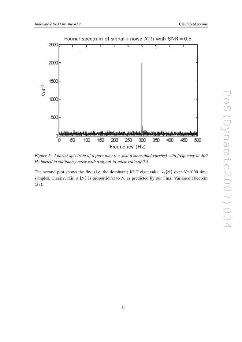
as a new function of N. And this derivative turns out to be a constant with respect to N. This fact paves the way to a new set of applications of the KLT to all fields of science! In fact, numeric simulations lead to the results shown in 4 plots below. The first plot is the ordinary Fourier spectrum of a pure tone at 300 Hz buried in noise with a signal-to-noise ratio of 0.5, abbreviated hereafter as SNR=0.5. For a definition of the SNR see the Wikipedia site http://en.wikipedia.org/wiki/Signal-to-noise_ratio. Please notice two facts: 1) This is about the lowest SNR below which the FFT starts failing to denoise a signal, a well-known fact to electrical and electronic engineers. 2) This Fourier spectrum is obviously computed by taking the Fourier transform of the stationary autocorrelation of X(t), as well-known from the Wiener-Khinchin Theorem (for a concise description of this theorem, see http://en.wikipedia.org/wiki/Wiener%E2%80%93Khinchin_theorem). Notice, however, that this procedure would not work for non-stationary X(t) because the Wiener-Khinchin Theorem does not apply to non-stationary processes. For non-stationary processes there are other “tricks” to compute the spectrum from the autocorrelation, like the Wigner-Ville Transform, but shall not consider them here.

PoS(Dynamic2007)034


11

Figure 1: Fourier spectrum of a pure tone (i.e. just a sinusoidal carrier) with frequency at 300 Hz buried in stationary noise with a signal-to-noise ratio of 0.5.

The second plot shows the first (i.e. the dominant) KLT eigenvalue ( )N1! over N=1000 time

samples. Clearly, this ( )N1! is proportional to N, as predicted by our Final Variance Theorem

(27).

PoS(Dynamic2007)034


12

Figure 2: The KLT dominant eigenvalue ( )N

1! over N=1000 time samples, computed by virtue

of the BAM, the Bordered Autocorrelation Method.

So, its derivative, ( )N

N

!

!1" , is a constant with respect to N. But we may then take the Fourier

transform of such a constant and clearly we get a Dirac delta function, i.e. a peak just at 300 Hz. In other words, we have KLT-reconstructed the original tone by virtue of the BAM. The third plot below shows such a BAM-reconstructed peak.

PoS(Dynamic2007)034


13

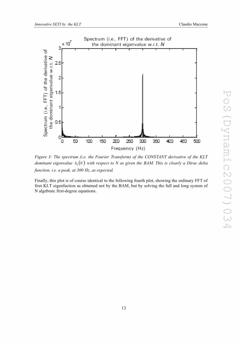
Figure 3: The spectrum (i.e. the Fourier Transform) of the CONSTANT derivative of the KLT dominant eigenvalue ( )N

1! with respect to N as given the BAM. This is clearly a Dirac delta

function, i.e. a peak, at 300 Hz, as expected.

Finally, this plot is of course identical to the following fourth plot, showing the ordinary FFT of first KLT eigenfuction as obtained not by the BAM, but by solving the full and long system of N algebraic first-degree equations.

PoS(Dynamic2007)034


14

Figure 4: The spectrum (i.e. the Fourier Transform) of the first KLT eigenfunction NOT obtained by the BAM, but rather by the very long procedure of solving the N linear algebraic equations corresponding, in discrete time, to the integral equation (18). Clearly, the result is the same as obtained in Figure 11.3 by the much less time-consuming BAM. So, one can say that the adoption of the BAM actually made the KLT “feasible” on small computers by circumventing the diffuculty of the N2 calculations requested by the “straight” KLT theory.

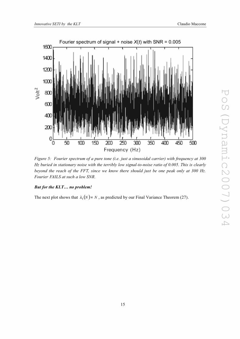
Let us now do the same again… but with an incredibly low SNR of 0.005. Poor Fourier here is in a mess! Just look at the next plot! No classical FFT spectrum can be identified at all for such a terribly low SNR!

PoS(Dynamic2007)034


15

Fourier spectrum of signal + noise X(t) with SNR = 0.005

Figure 5: Fourier spectrum of a pure tone (i.e. just a sinusoidal carrier) with frequency at 300 Hz buried in stationary noise with the terribly low signal-to-noise ratio of 0.005. This is clearly beyond the reach of the FFT, since we know there should just be one peak only at 300 Hz. Fourier FAILS at such a low SNR.

But for the KLT… no problem! The next plot shows that ( ) NN !

1" , as predicted by our Final Variance Theorem (27).

PoS(Dynamic2007)034


16

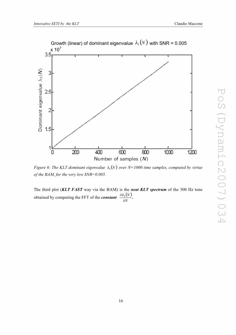
Growth (linear) of dominant eigenvalue ( )N

1! with SNR = 0.005

x 107

Figure 6: The KLT dominant eigenvalue ( )N

1! over N=1000 time samples, computed by virtue

of the BAM, for the very low SNR=0.005.

The third plot (KLT FAST way via the BAM) is the neat KLT spectrum of the 300 Hz tone

obtained by computing the FFT of the constant ( )N

N

!

!1" .

PoS(Dynamic2007)034


17

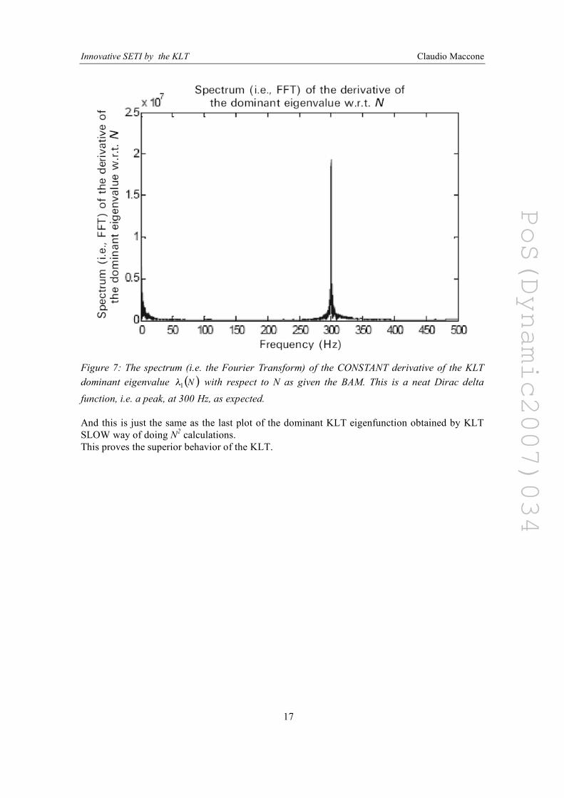
Figure 7: The spectrum (i.e. the Fourier Transform) of the CONSTANT derivative of the KLT dominant eigenvalue ( )N

1! with respect to N as given the BAM. This is a neat Dirac delta

function, i.e. a peak, at 300 Hz, as expected.

And this is just the same as the last plot of the dominant KLT eigenfunction obtained by KLT SLOW way of doing N2 calculations. This proves the superior behavior of the KLT.

PoS(Dynamic2007)034


18

Figure 8: The spectrum (i.e. the Fourier Transform) of the first KLT eigenfunction NOT obtained by the BAM, but rather by the very long procedure of solving the N linear algebraic equations corresponding, in discrete time, to the integral equation (18). Clearly, the result is the same as obtained in Figure 11.7 by the much less time-consuming BAM. So, one can say that the adoption of the BAM actually made the KLT “feasible” on small computers by circumventing the difficulty of the N2 calculations requested by the “straight” KLT theory.

7. Conclusions

Let us firstly summarize the results mathematically described in the last, key section for practical applications of the KLT to stationary processes.

When the stochastic process X(t) is stationary (i.e. it has both mean value and variance constant in time), then there are two alternative ways to compute the first KLT dominant eigenfunction (that is the roughest approximation to the full KLT expansion, that may be “enough” for practical applications!):

1) (Long Way) Either you compute the first eigenvalue from the autocorrelation and Fourier-transform it to get the first eigenfunction, or

2) (Short Way = BAM) You compute the derivative of the first eigenvalue with respect to T=N and then Fourier-transform it to get the first eigenfunction.

In practical numerical simulations of the KLT it may be much less time-consuming to choose option 2) rather than option 1).

Secondly, and most important, in either case, the KLT of a given stationary process can retrieve a sinusoidal carrier out of the noise for values of the signal-to-noise ratio (SNR) that are three orders of magnitude lower than those that the FFT can still filter out. In other words, while the

PoS(Dynamic2007)034


19

FFT (at best) can filter out signals buried in a noise that as a SNR of about 1 or so, the KLT can, say, filter out signals that have a SNR of, say, 0.001 or so.

This is the superior achievement of the KLT with respect to the FFT.

8. SETI for LOFAR and the SKA by virtue of the KLT

Let us finally look at the future of SETI. Two important projects are under development: LOFAR, described at the Wikipedia site http://en.wikipedia.org/wiki/LOFAR and the SKA, see http://en.wikipedia.org/wiki/Square_Kilometre_Array. Both will probably be used for SETI too.

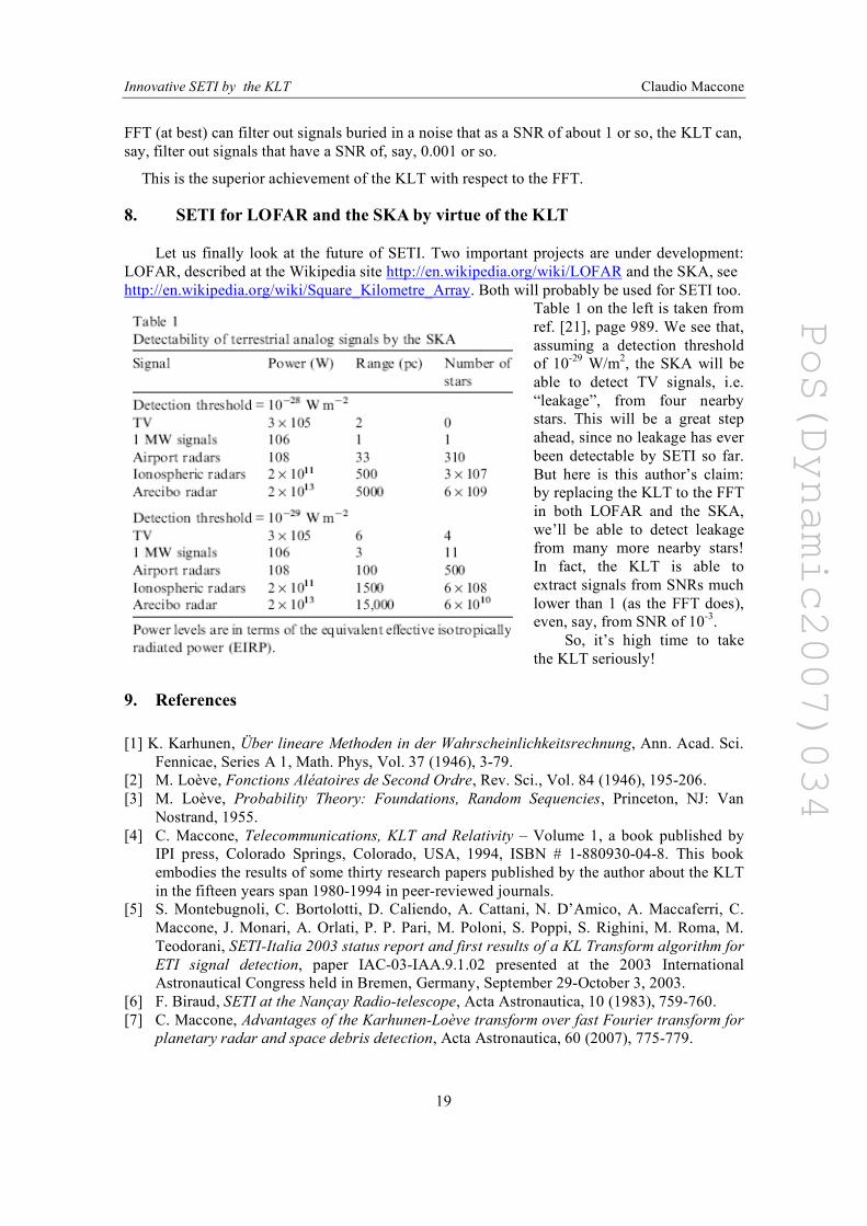
Table 1 on the left is taken from ref. [21], page 989. We see that, assuming a detection threshold of 10-29 W/m2, the SKA will be able to detect TV signals, i.e. “leakage”, from four nearby stars. This will be a great step ahead, since no leakage has ever been detectable by SETI so far. But here is this author’s claim: by replacing the KLT to the FFT in both LOFAR and the SKA, we’ll be able to detect leakage from many more nearby stars! In fact, the KLT is able to extract signals from SNRs much lower than 1 (as the FFT does), even, say, from SNR of 10-3. So, it’s high time to take the KLT seriously!

9. References [1] K. Karhunen, Über lineare Methoden in der Wahrscheinlichkeitsrechnung, Ann. Acad. Sci.

Fennicae, Series A 1, Math. Phys, Vol. 37 (1946), 3-79. [2] M. Loève, Fonctions Aléatoires de Second Ordre, Rev. Sci., Vol. 84 (1946), 195-206. [3] M. Loève, Probability Theory: Foundations, Random Sequencies, Princeton, NJ: Van

Nostrand, 1955. [4] C. Maccone, Telecommunications, KLT and Relativity – Volume 1, a book published by

IPI press, Colorado Springs, Colorado, USA, 1994, ISBN # 1-880930-04-8. This book embodies the results of some thirty research papers published by the author about the KLT in the fifteen years span 1980-1994 in peer-reviewed journals.

[5] S. Montebugnoli, C. Bortolotti, D. Caliendo, A. Cattani, N. D’Amico, A. Maccaferri, C. Maccone, J. Monari, A. Orlati, P. P. Pari, M. Poloni, S. Poppi, S. Righini, M. Roma, M. Teodorani, SETI-Italia 2003 status report and first results of a KL Transform algorithm for ETI signal detection, paper IAC-03-IAA.9.1.02 presented at the 2003 International Astronautical Congress held in Bremen, Germany, September 29-October 3, 2003.

[6] F. Biraud, SETI at the Nançay Radio-telescope, Acta Astronautica, 10 (1983), 759-760. [7] C. Maccone, Advantages of the Karhunen-Loève transform over fast Fourier transform for

planetary radar and space debris detection, Acta Astronautica, 60 (2007), 775-779.

PoS(Dynamic2007)034


20

Annotated Bibliography. In addition to the above References, we would like to offer an enlightened list of a few key references about the KLT, subdivided according to the field of application. We start by listing some early papers by the author about the KLT:

1) Il Nuovo Cimento: [8] C. Maccone, Special Relativity and the Karhunen-Loève Expansion of Brownian Motion,

Nuovo Cimento, Series B, Vol. 100 (1987), 329-342. 2) Bollettino dell’Unione Matematica Italiana:

[9] C. Maccone, Eigenfunctions and Energy for Time-Rescaled Gaussian Processes, Bollettino dell’Unione Matematica Italiana, Series 6, Vol. 3-A (1984), 213-219.

[10] C. Maccone, The Time-Rescaled Brownian Motion B(t2H), Bollettino dell’Unione Matematica Italiana, Series 6, Vol. 4-C (1985), 363-378.

[11] C. Maccone, The Karhunen-Loève Expansion of the Zero-Mean Square Process of a Time-Rescaled Gaussian Process, Bollettino dell’Unione Matematica Italiana, Series 7, Vol. 2-A (1988), 221-229.

3) Journal of the British Interplanetary Society: [12] C. Maccone, Relativistic Interstellar Flight and Genetics, Journal of the British

Interplanetary Society, Vol. 43 (1990), 569-572. 4) Acta Astronautica:

[13] C. Maccone, Relativistic Interstellar Flight and Gaussian Noise, Acta Astronautica, Vol. 17, No. 9 (1988), 1019-1027.

[14] C. Maccone, Relativistic Interstellar Flight and Instantaneous Noise Energy, Acta Astronautica, Vol. 21, No. 3 (1990), 155-159.

KLT for Data Compression: [15] C. Maccone, The Data Compression Problem for the Gaia Astrometric Satellite of ESA,

Acta Astronautica, Vol. 44 (1999), Nos. 7-12, 375-384. Some important papers about the KLT for SETI: [16] R. S. Dixon and M. Klein. On the detection of unknown signals, Proceedings of the Third

decennial US-USSR Conference on SETI held at the University of California at Santa Cruz, August 5-9, 1991. Later published in the Astronomical Society of the Pacific (ASP) Conference Series (Seth Shostak, editor) Vol. 47 (1993), 128-140.

[17] C. Maccone, Karhunen-Loève Versus Fourier Transform for SETI, Lecture Notes in Physics, Springer-Verlag, Vol. 390 (1990), 247-253. These are the Proceedings (Jean Heidmann and Mike Klein, editors) of the Third Bioastronomy Conference held at Val Cenis, Savoie, France, 18-23 June 1990.

After these seminal works were published, the importance of the KLT for SETI was finally acknowledged by the SETI Institute experts in: [18] SETI 2020, Ron Eckers, Kent Cullers, John Billingham and Lou Scheffer editors, SETI

Institute, 2002, 234, note 13. The authors say: Currently (2002) only the Karhunen Loeve (KL) transform [Mac94] shows potential for recognizing the difference between the incidental radiation technology and white noise. The KL transform is too computationally intensive for present generation of systems. The capability for using the KL transform should be added to future systems when the computational requirements become affordable. The paper [Mac94] referred to in the SETI 2020 statement mentioned above is:

[19] C. Maccone, The Karhunen-Loève Transform: A Better Tool than the Fourier Transform for SETI and Relativity, Journal of the British Interplanetary Society, Vol. 47 (1994), p. 1.

An early paper about the possibility of a Fast KLT: [20] A. K. Jain, A Fast Karhunen-Loève Transform for a Class of Random Processes, IEEE

Trans. Commun. COM-24, 1976, 1023-1029. A recent paper about the future SETI by virtue of the SKA: [21] T. Joseph W. Lazio, Jill C. Tarter, D. J. Wilner, The Cradle of life, New Astronomy

Reviews, Vol. 48 (2004), p. 985-991.

Innovative SETI by the KLT

Documents

Transcript of Innovative SETI by the KLT