1
Innovative NDT technique based on ferrofluids for detection of surface cracks
J.I. Rojasa,1, B. Cabreraa, G. Musternia, J. Nicolasa, J. Tristanchoa,2, and D. Crespoa,3 a Universitat Politècnica de Catalunya, Escola d’Enginyeria de Telecomunicació i Aeroespacial de Castelldefels,
C/ Esteve Terradas 7, 08860, Castelldefels, Spain 1 corresponding author: email: josep.ignasi.rojas@upc.edu; tel.: +34 93 413 4130; fax: +34 93 413 7007 2 email: joshua.tristancho@upc.edu 3 email: daniel.crespo@upc.edu
Abstract
An innovative NDT technique is proposed for surface inspection of materials not necessarily
magnetic or conductive, based on local magnetic field variations due to ferrofluid deposited in
the cracks. The feasibility of the technique is assessed preliminarily, based on signal
detectability without applied external magnetic field, and under applied DC fields. The signals
(local magnetic flux density variations) are quantified analytically, experimentally and
numerically. The model agrees well with the tests, showing that the signal increases with the
applied field strength, up to the saturation magnetization of the ferrofluid, and decreases with
the distance to the crack longitudinal axis, and thus it can provide useful estimations of the
signal. The proposed technique, requiring application of external fields to magnetize the
ferrofluid to enhance the signal, seems promising: the model suggests that signals associated
to cracks significantly smaller than surface cracks in a target application like aircraft skin
panel inspection NASA STD-5009 are easily detectable with commercial magnetometers.
Keywords: surface flaw; magnetic particle; ferrofluid; aluminium alloys; composite materials
1. INTRODUCTION
Early crack detection and monitoring is critical for, inter alia, aviation safety and, for this
purpose, Non-Destructive Testing (NDT) is an indispensable tool in both production and
maintenance. That is why the aerospace sector is one of the largest customers for the NDT
industry: in 2008 and 2010, the global expenditure on NDT equipment was slightly over $1
billion [1,2], and was forecasted to grow up to $1.3 billion by 2013 [2], and $1.4 billion by
2017 [1]. Thus, research on NDT solutions for aerospace components that enhance safety and
reduce costs is of paramount importance for the NDT and aerospace industries.
2
In this work, an innovative NDT technique is proposed for surface inspection, based on
detection of local magnetic field variations due to accumulation of a ferrofluid in surface
cracks. Ferrofluids are colloidal suspensions of small surfacted magnetic particles in a liquid
carrier [3]; typically, iron oxide nanoparticles in a Newtonian fluid that can be polar (water)
or non-polar (organic solvents). Ferrofluids can be magnetized by applying an external
magnetic field, as it forces the magnetic dipole moments of the particles in suspension to align
with the direction of the applied field [3]. The objective of this work is to make a preliminary
assessment of the feasibility of the proposed NDT technique, based on signal detectability
without applied magnetic fields, and under applied direct current (DC) magnetic fields. For
this purpose, investigations are conducted to quantify analytically, experimentally and
numerically the local magnetic field variations due to presence of a ferrofluid in surface
cracks machined in plates of aluminium alloy (AA) 2024-T3. This alloy was chosen as it is
widely used in applications for which fatigue resistance is critical, like in skin panels of
military aircraft [4] and commercial civil aviation aircraft [5]. The ultimate goal of this
research is to implement the proposed technique, meeting the accuracy, reliability and safety
requirements of NDT applications in the aerospace industry, while trying to reduce the
inspection costs. The latter can be achieved through a combination of reductions in equipment
cost, inspection time, operator training, etc., while guaranteeing suitability to a wide range of
aerospace NDT applications. Namely, the proposed technique would be applicable for surface
inspection of materials not necessarily magnetic or conductive, e.g., aluminium alloys and
Carbon or Glass Fibre Reinforced Polymers.
1.1 Dimensions of the studied cracks
The minimum detectable crack depends on the inspection method [6]. In aircraft structural
design, the initial crack depends on the component and the type of flaw evaluated [7].
Namely, for fail-safe involving surface flaws, an initial damage of 1.27 mm (3.18 mm for
slow-flaw growth) is assumed for pre-service inspections with high standard NDT, while 6.35
mm is assumed for in-service inspections. In structural applications of aluminium alloy panels
in aircraft, the most common NDT method for crack monitoring is General Visual Inspection
(GVI) [8]. For GVI, the length of the detectable crack ranges from 5.08 to 12.70 mm. For
other NDT techniques comparable to the subject of this work, the minimum detectable surface
crack is: 1) for dye penetrant testing (PT), 6.36 mm long, 0.64 mm deep, or 3.82 mm long,
1.91 mm deep; 2) for eddy current testing (ET), 5.08 mm long, 0.51 mm deep, or 2.54 mm
long, 1.27 mm deep; and 3) for magnetic particle testing (MT), 9.56 mm long, 0.97 mm deep,
3
or 6.36 mm long, 1.91 mm deep [6]. Our purpose is to determine if the proposed NDT
concept would allow detection of surface cracks with these dimensions or smaller, given that
one of the target applications is aircraft skin panel inspection. However, for the preliminary
study for the proof of concept, cracks of larger dimensions were used. Once the experimental
measurements validated the model results for the local magnetic field variations, further
computations were made for cracks with the aforementioned dimensions.
2. MATERIALS & METHODS
2.1 Tested specimens
The tested specimens are rectangular plates 100 mm long, 20 mm wide and 2 mm thick,
machine cut from sheet of as-received commercial AA 2024-T3. The thickness matches
typical values for aircraft skin panels, e.g., 1–1.6 mm for plain panels without holes and 2–3
mm for heavy loaded panels like those in the wing [9]. Using a metal saw, simulated cracks
were machined in the surface of the samples along the longitudinal symmetry axis. Simulated
cracks can be used in research instead of real cracks grown by fatigue during operation or
dynamic testing [10]. The reference crack was 60 mm in length , 1.50 mm in width , and
0.70 mm in depth . In subsequent series of tests, cracks with in the range 34.86–66.40 mm,
in the range 1.97–2.85 mm, and in the range 0.52–0.65 mm were used. Finally, for the
transversal tests, a crack 12.75 mm long, 0.95 mm wide and 0.60 mm deep, machined in a
plate 20 mm long, 20 mm wide, was used.
2.2 Ferrofluids
The magnetic particles in ferrofluids are generally spherical and with diameters ranging from
5 to 15 nm [3,11,12]. Also, each particle is generally a single magnetic domain, i.e., it is an
entity with a single magnetic moment, and thus behaves as a single magnetic dipole. The
volume fraction of ferrofluids, i.e., the volume percentage of magnetic solid material with
respect to the total volume, is usually 5 to 15%. Four ferrofluids have been considered: three
generic suspensions of ferromagnetic nanoparticles and the commercial ferrofluid N-503 from
Sigma Hi-Chemical Inc. (the properties of the latter are shown in Table 1, as provided by the
manufacturer). The generic suspensions are made of iron (α-Fe), magnetite (Fe3O4) and
maghemite (γ-Fe2O3) nanoparticles, respectively (their properties are shown in Table 2). For
simplicity, the idea of synthesizing a custom-made ferrofluid was disregarded and it was
decided to use only the commercial ferrofluid for the experiments, and consequently also for
4
the numerical simulations. Nevertheless, for comparison purposes, the theoretical
development and calculations in Section 3 were applied to all four ferrofluids.
Table 1 Properties of commercial ferrofluid N-503 supplied by Sigma Hi-Chemical Inc.
Concept Value Liquid carrier Iso-paraffin Type of magnetic particles Magnetite (Fe3O4) particles Average diameter 10 nm Volume fraction 8.9% Saturation magnetization 43.8 kA/m Dynamic viscosity 20.6 mPa·s, at 293 K
Table 2 Properties of iron (α-Fe), magnetite (Fe3O4) and maghemite (γ-Fe2O3) particles at room temperature (RT).
Type Concept Value Reference Observations α-Fe Critical diametera 7 nm [13] Mass/specific saturation
magnetization 91.3 A·m2/kg [14] 8.4 nm diameter particles
Density 7870 kg/m3 Fe3O4 Critical diametera 128 nm Mass/specific saturation
magnetization 46 A·m2/kg [15] 19 nm diameter particles
Density 5000 kg/m3 γ-Fe2O3 Critical diametera 166 nm Mass/specific saturation
magnetization 36.6 A·m2/kg [16] 9 nm diameter particles
Density 4600 kg/m3 a The critical diameter is a threshold below which a magnetic particle is a single magnetic domain. Above this critical diameter, the particle consists of multiple magnetic domains.
2.3 Experimental setup & methodology
The magnetic flux density was measured before and during application of a DC magnetic
field, with and without ferrofluid in the reference crack. Fig. 1 shows the experimental set.
The custom-made bracket (see Appendix A and Online Resource 1) consists of two concentric
Cu wire coils covered by a protective shell, and the specimen support, located such that the
crack in the sample is aligned with the revolution axes of the coils. A dispenser was used for
depositing the ferrofluid in the cracks. A power source supplied DC power to the coils for
generating DC magnetic fields. The intensity and voltage of the current were measured with a
multimeter, while was measured with the AlphaLab magnetometer (with resolution 0.001
mT and accuracy ± 2%). The reference position of the Hall probe was 3.5 mm below the
crack centre, oriented to measure the component of in the direction of the revolution axes of
the coils. Measurements were taken sequentially in a series of cases summarized in Table 3.
5
For the cases where power is supplied to the coils, the tested voltages ranged from 1 to 17 V,
with the coils generating applied external fields with strengths ranging from around 1 to 16
kA/m. Higher applied fields were not used because the gain in ferrofluid magnetization is
counterbalanced by a much poorer magnetometer resolution for the signals above 20 mT.
For another sample, tests were realized with the Hall probe located at increasing distance from
the crack, with of 8 kA/m. Also, tests with surface cracks of different dimensions were
conducted, with the Hall probe located back in the reference position, with of 8 and 16
kA/m. Finally, tests were made with a crack oriented perpendicular to the revolution axes of
the coils, and thus to the applied field, to explore the response if the defect does not lay
parallel to this field. In this case, the crack and plate were smaller to allow introducing the
plate inside the support transversally. The tests were performed in a laboratory with low
electromagnetic noise. Prior to testing, the background field was zeroed by applying an
appropriate offset in the magnetometer. Each of the test results shown in Section 4 is the
average of three individual measurements (the error bars in the figures represent one standard
deviation).
Fig. 1 Experimental set: ferrofluid (1), test specimen (2), magnetometer and Hall probe (3), custom-made bracket (4), multimeter (5), power source (6) and connection cables (7)
Table 3 Summary of experimental conditions applied sequentially during the tests.
DC test cases Sample on support Ferrofluid in the crack DC power supplied to coils DC.1 No No No DC.2 Yes No No DC.3 Yes No Yes DC.4 Yes Yesa No (before magnetizing) DC.5 Yes Yesa Yes (ferrofluid magnetized) a Namely, the volume of commercial ferrofluid in the reference crack is approximately 50 mm3.
6
2.4 Simulations with COMSOL Multi-physics
The local magnetic field variations due to the presence of ferrofluid in the reference crack
were computed numerically with the AC/DC Module of COMSOL Multi-physics, a
commercial finite element analysis software package for coupled physics phenomena and
engineering applications, developed by COMSOL, Inc., Palo Alto, CA, USA. The mesh was a
user-controlled unstructured 3D mesh of tetrahedral elements. The properties of the ferrofluid,
the air and the test plates used in the simulations are summarized in Table 4. The electrical
conductivity, permittivity and permeability of the commercial ferrofluid were not supplied by
the manufacturer. The conductivity, measured with a Hach HQ440d Multi-Parameter Meter,
was 5×10-5 S/m. The relative permittivity used in the simulations was that of the iso-paraffin.
The relative permeability ( = 83.6) resulted from a calibration based on fitting the
simulation results to the measured field in the probe position under an applied DC field of 16
kA/m. The solver selected for the simulations was the iterative FGMRES.
Table 4 Properties of the ferrofluid, air and AA 2024-T3 at 293 K, as used in COMSOL simulations.
Material Electrical conductivity (S/m) Relative permittivity (-) Relative permeability (-) Magnetite Iso-paraffin Ferrofluid
9.61×108 [17] Insulator 0 (measured)a
15 [18], 33.7–81 [19] 1.9 [20] 2
1.4–2.0 [18] – 1.5–6 [21], 3–96 [22]
Air 0 (COMSOL database)a 1 (COMSOL database) 1 (COMSOL database) AA 2024-T3 1.60×107 – 1.89×107 [23] 1.44 [24], 8.0 [25] 1.00002 [26] a The electrical conductivity measured for the commercial ferrofluid was 0 S/m, and the conductivity for air in COMSOL’s materials database is 0 S/m. This is reported to cause problems in the solver. Instead, it is recommended to use a very small conductivity value, and so 10 S/m was used.
3. THEORY & CALCULATIONS
The ferrofluid in the crack is modelled as a magnetic dipole with semi-length and radius ,
such that it has the length of the crack and a volume equal to the volume of ferrofluid placed
in the crack. The origin of the reference system used in this work is the dipole centre. The z
axis is the revolution axis of the dipole, parallel to the crack and revolution axes of the coils.
The y axis is perpendicular to the z axis, pointing opposite to gravity (see Online Resource 1).
3.1 Equilibrium (DC) magnetization of the ferrofluid
Ferrofluids can be magnetized by external DC magnetic fields [3]. This phenomenon
increases with , up to reaching [27]. The following hypotheses are assumed:
1. The ferrofluid is mono-disperse, i.e., the particles are all identical in properties,
composition, dimensions and shape (assumed spherical, with diameter 10 nm).
7
2. For being conservative, the generic ferrofluids are considered dilute colloidal
suspensions with volume fraction of 7%, and is the smallest in the literature
for the corresponding type of particles (see Table 2).
3. Each magnetic particle is a single magnetic domain. This is coherent with the
critical diameters found for the studied ferrofluids (see Table 2).
4. The magnetization is homogeneous within the ferrofluid.
5. The magnetic particles in suspension are isotropic and non-interacting.
If a ferrofluid is a collection of individual, non-interacting and mono-disperse magnetic
dipoles, a theory by Langevin [3] states that, under a field applied in the z axis, the ferrofluid
non-dimensional magnetization along that axis is = ⁄ = coth( )− 1⁄ , with the
Langevin parameter = ⁄ , where is the magnetic moment of the particles
(15.5×10−19 A·m2, for magnetite [28]), is the free space permeability constant, is the
Boltzmann constant, and is the temperature. Fig. 2 shows the magnetization curve
computed for the commercial ferrofluid at 293 K. If the applied field is suppressed, relaxes
to a new equilibrium state following an exponential decay being = exp(− ⁄ ), where
is the relaxation time [3].
Fig. 2 Magnetization of the ferrofluid vs. applied field strength , at 293 K, by Langevin’s theory [3]
3. 2 Magnetic field of the ferrofluid
For applied DC fields or absence of applied field, crack detection would be based on the local
variations of due to the ferrofluid in the crack. A magnetic field can be calculated with
Maxwell’s equations [29]: ( ) = ( ) + ( ) = ( ) − ∇ ∗( ), where is the
position vector of the point where the field is evaluated, is the magnetization, and ∗ is a
8
scalar potential. Inside the dipole, depends on the ferrofluid magnetization. Outside the
dipole, is associated to the electromagnetic noise. In this work, this term is null in the z
axis due to the offset applied to the magnetometer prior to testing. Thus, the magnetic flux
density associated to the ferrofluid is [29]:
Eq. 1 ( ) = − ∇ ∗( ) = − ∇ ∫ ( ′) · | |
d ′
where is the volume of magnetized material (i.e., the volume of ferrofluid) and ′ is the
position vector of a differential magnetic dipole. If the ferrofluid in the crack is modelled as a
cylindrical dipole with semi-length and radius , when the applied field is aligned with the
dipole longitudinal axis, i.e., the z axis, Eq. 1 becomes:
Eq. 2
2 ) ]
To explore the response if the applied field is perpendicular to the crack/dipole longitudinal
axis, the dipole is rotated 90º to align it with the x axis. Then, Eq. 1 becomes:
Eq. 3 ( ) = − [( (( ) ) ( )
3.3 Magnetic field of the ferrofluid in the xy plane
After preliminary computations with Eq. 2, the field associated to the ferrofluid was observed
to be very significant in the z axis close to the dipole tip (see Online Resource 2), but it is not
possible to take measurements there. Also, the field vanishes dramatically with the distance to
the z axis, and the direction of the field lines changes significantly in short distances. Thus, it
9
is very complex to establish the most appropriate position and orientation of the probe if it is
to be placed in the vicinity of the tip of the crack/dipole but separated from the z axis (the
magnetometer is only able to measure the field in one direction). Conversely, in the xy plane
the field is expected to have component only in the z axis, , which facilitates taking
measurements. For these reasons, the study was focused on the xy plane, where the signal
when the applied field is aligned with the dipole longitudinal axis, as obtained from Eq. 2, is:
Eq. 4 | ( )| = = − ( )
For the reference crack, modelled by a dipole with a of 30 mm and of 0.51 mm (see Online
Resource 1), Fig. 3 shows as obtained from Eq. 4 for the generic ferrofluids and the
commercial ferrofluid, all at their . On the other side, if the applied field is perpendicular
to the dipole longitudinal axis, from Eq. 3, the signal in the xy plane is:
Eq. 5 | ( )| = = − (( ) )
− (( ) )
Fig. 3 For the reference crack (modelled by a dipole with of 30 mm and of 0.51 mm), analytical vs. x and y coordinates, in the xy plane, for ferrofluids made of a) iron (α-Fe) nanoparticles, b) magnetite (Fe3O4) nanoparticles, c) maghemite (γ-Fe2O3) nanoparticles, and d) for the commercial ferrofluid, all at their
10
Measurements under DC.1 test conditions provided the background magnetic field in the
laboratory. Then, the magnetometer reading was set to zero by applying appropriate offset.
Measurements under DC.2 test conditions served for establishing a baseline for identifying
variations of due to presence of ferrofluid in the crack before supplying DC power to the
coils (i.e., before magnetizing the ferrofluid). These measurements also confirmed that the
samples do not modify the background field, as expected since AA 2024-T3 is diamagnetic.
Analogously, measurements under DC.3 test conditions served for establishing a baseline for
identifying variations of while supplying DC power to the coils (i.e., while the ferrofluid is
being magnetized by application of an external DC field). Measurements under DC.4 and
DC.5 test conditions allowed computing the variations of in two different hypothetical
versions of the NDT technique:
Tech-DC.I: Variation of due to presence of ferrofluid in the crack when
the ferrofluid has not been previously magnetized: For the reference crack, this
variation (the difference between measurements obtained in cases DC.4 and
DC.2) could not be determined, since the fields are below the sensor resolution.
Tech-DC.II: Variation of due to presence of ferrofluid in the crack when
the ferrofluid is being magnetized: For the reference crack, Fig. 4 shows this
variation (the difference between measurements obtained in cases DC.5 and
DC.3), and also the model results derived from the theoretical development in
Section 3, where the ferrofluid magnetization increases with . Although the test
results show high dispersion, probably due to errors in measuring the crack size
and the volume of ferrofluid deposited from test to test, the average error of the
model results is -2.2 ± 51.2 % and both follow the same trend.
4.1 Comparison of test results for Tech-DC.I and Tech-DC.II
For the version Tech-DC.I, the local variation of due to the ferrofluid when it has not been
previously magnetized is below the minimum resolution of the AlphaLab magnetometer. As
expected, the signal is much more significant for the version Tech-DC.II, and increases with
since the ferrofluid equilibrium magnetization also increases [27]. The variation for the
highest tested field is -7 μT. Although according to the theory it should be the maximum
signal, it is not the case (the highest measured variation is -9.7 μT, for of 14.5 kA/m),
probably due to experimental error. The maximum signal-to-noise ratio is -69 dB,
11
corresponding to a variation of -5 μT, achieved for the smallest . An NDT technique based
on the version Tech-DC.II would require the operator to scan at least two times the inspection
surface: first to clean the surface and spread the ferrofluid (a likely drawback is that the
surface has to be clean and the cracks must not be polluted, like for PT), and second to apply
the external field while measuring the response. Thus, the inspection equipment should be
able to simultaneously generate a field to magnetize the ferrofluid (preferably up to ,
from the basis of signal detectability), and to measure the local variations of . Crack
detection capabilities can be enhanced using higher sensitivity sensors (magnetometers with
resolutions down to 0.1 nT are common) or ferrofluids with higher . Finally, a 3-
components Hall probe would be more appropriate, since the operator in an NDT inspection
does not know the crack orientation and the direction in which the induced field is higher.
Fig. 4 For version Tech-DC.II at 293 K for the reference crack, analytical and measured variation of (difference between measurements obtained in cases DC.5 and DC.3) vs. applied field strength (case DC.3), for the commercial ferrofluid, with the Hall probe located at 3.5 mm from the dipole axis
4.2 Comparison of model results with test results for Tech-DC.II
The model results in the xy plane (see Eq. 4 and Fig. 3) show that, as expected, the absolute
value of the variation of due to the ferrofluid in the crack decreases with the distance to the
dipole axis in the xy plane = + . For sample #2 (see crack dimensions in Table 5),
tests were made with the Hall probe located at increasing distance from the dipole axis
(namely, at 3.5, 7.5 and 11.5 mm), with of 8 kA/m. Fig. 5 shows the measured signal, i.e.,
the variation of due to presence of ferrofluid in the crack when the ferrofluid is being
magnetized (the difference between measurements in cases DC.5 and DC.3), compared to
model results. Model results for slightly above 700 kA/m are also shown, as a
12
representative condition at which the ferrofluid has reached . The tests confirm that the
signal decreases with , but apparently at a slightly slower rate to that shown by the model
(the error of the model increases with , and in average it is -13.7 ± 3.0 %). As expected, the
sensor should always be placed as close as possible to the inspection surface.
Fig. 5 For version Tech-DC.II at 293 K for sample #2, analytical and measured variation of (difference between measurements obtained in cases DC.5 and DC.3) vs. distance to dipole axis in the xy plane , for the commercial ferrofluid, for applied field strength of 8 and 716 kA/m (ferrofluid at )
To further validate the model, tests with surface cracks of different dimensions were made,
with the Hall probe located back in the reference position, with of 8 and 16 kA/m. Table 5
shows the measured signals compared to model results. Finally, Table 6 shows the model
results and test results (again, the difference between readings in cases DC.5 and DC.3) for a
crack perpendicular to the applied field, with the Hall probe placed at 5.5 mm from the dipole
axis. The signals measured for the crack oriented in the direction of the applied external field
and perpendicular to it are virtually identical in spite of the distance to the crack being larger
in the second case. On the other side, the signal predicted by the model is significantly higher
if the defect lays perpendicular to the applied field. Thus, the model seems not so appropriate
to estimate the signal for the latter condition. However, the test results suggest that not
knowing the direction of the defect when applying the external field may not be very relevant
to the performance of the proposed NDT method.
13
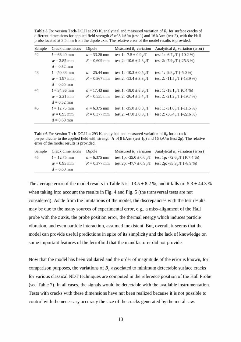
Table 5 For version Tech-DC.II at 293 K, analytical and measured variation of for surface cracks of different dimensions for applied field strength of 8 kA/m (test 1) and 16 kA/m (test 2), with the Hall probe located at 3.5 mm from the dipole axis. The relative error of the model results is provided.
Sample Crack dimensions Dipole Measured variation Analytical variation (error) #2 = 66.40 mm = 33.20 mm test 1: -7.5 ± 0.9 μT test 1: -6.7 μT (-10.2 %) = 2.85 mm = 0.609 mm test 2: -10.6 ± 2.3 μT test 2: -7.9 μT (-25.3 %) = 0.52 mm #3 = 50.88 mm = 25.44 mm test 1: -10.3 ± 0.5 μT test 1: -9.8 μT (-5.0 %) = 1.97 mm = 0.567 mm test 2: -13.4 ± 3.3 μT test 2: -11.5 μT (-13.9 %) = 0.65 mm #4 = 34.86 mm = 17.43 mm test 1: -18.0 ± 8.6 μT test 1: -18.1 μT (0.4 %) = 2.21 mm = 0.535 mm test 2: -26.4 ± 3.4 μT test 2: -21.2 μT (-19.7 %) = 0.52 mm #5 = 12.75 mm = 6.375 mm test 1: -35.0 ± 0.0 μT test 1: -31.0 μT (-11.5 %) = 0.95 mm = 0.377 mm test 2: -47.0 ± 0.8 μT test 2: -36.4 μT (-22.6 %) = 0.60 mm Table 6 For version Tech-DC.II at 293 K, analytical and measured variation of for a crack perpendicular to the applied field with strength of 8 kA/m (test 1p) and 16 kA/m (test 2p). The relative error of the model results is provided.
Sample Crack dimensions Dipole Measured variation Analytical variation (error) #5 = 12.75 mm = 6.375 mm test 1p: -35.0 ± 0.0 μT test 1p: -72.6 μT (107.4 %) = 0.95 mm = 0.377 mm test 2p: -47.7 ± 0.9 μT test 2p: -85.3 μT (78.9 %) = 0.60 mm
The average error of the model results in Table 5 is -13.5 ± 8.2 %, and it falls to -5.3 ± 44.3 %
when taking into account the results in Fig. 4 and Fig. 5 (the transversal tests are not
considered). Aside from the limitations of the model, the discrepancies with the test results
may be due to the many sources of experimental error, e.g., a miss-alignment of the Hall
probe with the z axis, the probe position error, the thermal energy which induces particle
vibration, and even particle interaction, assumed inexistent. But, overall, it seems that the
model can provide useful predictions in spite of its simplicity and the lack of knowledge on
some important features of the ferrofluid that the manufacturer did not provide.
Now that the model has been validated and the order of magnitude of the error is known, for
comparison purposes, the variations of associated to minimum detectable surface cracks
for various classical NDT techniques are computed in the reference position of the Hall Probe
(see Table 7). In all cases, the signals would be detectable with the available instrumentation.
Tests with cracks with these dimensions have not been realized because it is not possible to
control with the necessary accuracy the size of the cracks generated by the metal saw.
14
Table 7 For version Tech-DC.II at 293 K, analytical variation of for the minimum detectable surface cracks for various NDT techniques, for applied field strength of 8 kA/m (test 1) and 16 kA/m (test 2).
NDT technique Crack dimensions Dipole Analytical variation Assumed initial damage in = 1.27 mm = 0.635 mm test 1: -18.7 μT fail-safe = 0.51 mma = 0.255 mm test 2: -21.9 μT = 0.51 mma Assumed initial damage in = 3.18 mm = 1.59 mm test 1: -37.0 μT fail-safe (slow-flaw growth) = 0.51 mma = 0.255 mm test 2: -43.5 μT = 0.51 mma Eddy current testing 1 & = 5.08 mm = 2.54 mm test 1: -41.6 μT general visual inspection 1 = 0.51 mm = 0.255 mm test 2: -48.8 μT = 0.51 mm Eddy current testing 2 = 2.54 mm = 1.27 mm test 1: -81.1 μT = 0.51 mm = 0.402 mm test 2: -95.3 μT = 1.27 mm Dye penetrant testing 1 = 6.36 mm = 3.18 mm test 1: -49.9 μT = 0.51 mma = 0.286 mm test 2: -58.7 μT = 0.64 mm Dye penetrant testing 2 = 3.82 mm = 1.91 mm test 1: -149.3 μT = 0.51 mma = 0.493 mm test 2: -175.5 μT = 1.91 mm Magnetic particle testing 1 = 9.56 mm = 4.78 mm test 1: -57.9 μT = 0.51 mma = 0.352 mm test 2: -68.0 μT = 0.97 mm Magnetic particle testing 2 = 6.36 mm = 3.18 mm test 1: -149.0 μT = 0.51 mma = 0.493 mm test 2: -175.1 μT = 1.91 mm General visual inspection 2 = 12.70 mm = 6.35 mm test 1: -22.0 μT = 0.51 mma = 0.255 mm test 2: -25.9 μT = 0.51 mma a In those cases in which there is no information about the width/depth of the corresponding minimum detectable surface crack, a value of 0.51 mm has been used in the simulations, since it is the minimum width/depth value for the minimum detectable surface cracks for the techniques considered.
From Eq. 4, for a given value of and (and thus radius of the dipole), it can be derived
that, for a given distance of the Hall probe to the dipole axis in the xy plane, , there is a
dipole semi-length providing maximum signal: = √2⁄ . For example, for a crack with
= = 0.51 mm, in the reference position of the probe ( of 3.5 mm), a maximum in the
signal would be obtained for of 2.47 mm. This trend can be observed in Table 7. Finally, the
model has been used to estimate the minimum detectable surface crack for the proposed NDT
technique. For instance, for of 8 kA/m, for a crack with of 0.001 mm and = = 0.51
mm, the signal would be -15.4 nT; for a crack with of 1.27 mm and = 0.005 mm
(corresponding to, e.g., = = 0.01 mm), the signal would be -7.2 nT; and for a crack with
of 0.012 mm and = 0.05 mm (corresponding to, e.g., = = 0.1 mm), the signal would
15
be -7.1 nT. All these signals would be perfectly detectable using magnetometers with
resolution down to 0.1 nT, which are commercially available and not uncommon. These
model estimations suggest that the proposed NDT method has a promising performance.
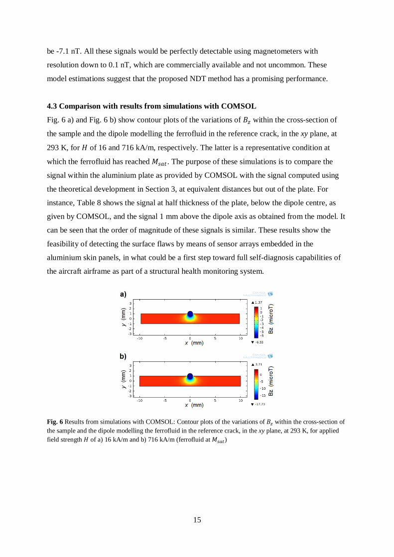
4.3 Comparison with results from simulations with COMSOL
Fig. 6 a) and Fig. 6 b) show contour plots of the variations of within the cross-section of
the sample and the dipole modelling the ferrofluid in the reference crack, in the xy plane, at
293 K, for of 16 and 716 kA/m, respectively. The latter is a representative condition at
which the ferrofluid has reached . The purpose of these simulations is to compare the
signal within the aluminium plate as provided by COMSOL with the signal computed using
the theoretical development in Section 3, at equivalent distances but out of the plate. For
instance, Table 8 shows the signal at half thickness of the plate, below the dipole centre, as
given by COMSOL, and the signal 1 mm above the dipole axis as obtained from the model. It
can be seen that the order of magnitude of these signals is similar. These results show the
feasibility of detecting the surface flaws by means of sensor arrays embedded in the
aluminium skin panels, in what could be a first step toward full self-diagnosis capabilities of
the aircraft airframe as part of a structural health monitoring system.
Fig. 6 Results from simulations with COMSOL: Contour plots of the variations of within the cross-section of the sample and the dipole modelling the ferrofluid in the reference crack, in the xy plane, at 293 K, for applied field strength of a) 16 kA/m and b) 716 kA/m (ferrofluid at )
16
Table 8 For version Tech-DC.II at 293 K for the reference crack, variations of obtained from the model and from the simulations with COMSOL for applied field strength of 16 kA/m (test 1) and 716 kA/m (test 2) at 1.0 mm from the dipole axis.
Sample Crack dimensions Dipole Numerical variation Analytical variation #1 = 60.00 mm = 30.00 mm test 1: -3.1 μT test 1: -6.9 μT = 1.50 mm = 0.510 mm test 2: -7.9 μT test 2: -7.9 μT = 0.70 mm
5. CONCLUSIONS
An innovative NDT technique is proposed for surface inspection of materials not necessarily
magnetic or conductive, based on detection of local magnetic field variations due to ferrofluid
deposited in the crack. A preliminary feasibility assessment is made, based on signal
detectability without applied magnetic field, and under applied DC fields. For this purpose,
the signals (local magnetic flux density variations) are quantified analytically, experimentally
and numerically for cracks in plates of AA 2024. The main conclusions are:
For the reference crack, filled with approximately 50 mm3 of ferrofluid, the
magnetic field of the ferrofluid in absence of an applied field is below the sensor
resolution. Detectable signals are obtained if the ferrofluid is being magnetized by
an external field. The signals increase with the applied field strength , e.g.,
reaching -7 μT at a distance of around 3.5 mm from the longitudinal axis of the
reference crack, for of 16 kA/m.
The model agrees well with the tests: the average error excluding the results for a
crack oriented perpendicular to the applied field is -5.3 %, and both follow similar
trends. For instance, the signal increases with up to the saturation magnetization
of the ferrofluid and, in a plane perpendicular to the crack longitudinal axis in the
crack centre, decreases with the distance to the axis. Thus, it is concluded that the
model can provide useful estimations of the signal.
The signals measured for a crack oriented in the direction of the applied external
field and perpendicular to it are virtually identical. This suggests that not knowing
the direction of the defect when applying the external field may not be relevant to
the performance of the proposed NDT method.
The proposed NDT technique, requiring application of DC external fields to
magnetize the ferrofluid to enhance the signal, seems promising: the model
suggests that signals associated to cracks significantly smaller than surface cracks
in a target application like aircraft skin panel inspection NASA STD-5009 are
easily detectable with commercial magnetometers.
17
Compared to PT, an advantage of the proposed NDT method is that it is
quantitative and, therefore, can be used to estimate the size of the cracks.
The use of non-commercial ferrofluids may provide some advantages like higher
, leading to more intense signals (this can be achieved using α-Fe particles),
or lower coercivity/hysteresis effects, or the possibility of developing ferrofluids
with tailored properties, like reduced viscosity and surface tension, making easier
for the ferrofluid to sip into the surface cracks, etc.
The ideas being considered for future work are: 1) to refine the research using, for instance, a
3-components Hall probe with higher sensitivity; 2) to correlate patterns in the local magnetic
field variations with crack morphology; 3) to study the applicability of the technique to detect
cracks in magnetic materials; 4) to study the effect of ferrofluid viscosity in crack penetration;
5) to study the feasibility of recycling classic eddy current equipment for implementing the
proposed NDT technique; 6) perform PT, ET, MT (if possible, depending on the tested
material) and tests with the proposed NDT method on small defects in the sub-mm range, to
establish the limits of the NDT technique; and finally 7) to study the performance of the
proposed technique upon application of AC fields. In AC, crack detection could be based on
the phase lag between the field close to the crack and the applied field. This approach has
inherent advantages: the phase lag, as opposed to , is independent of and the quantity of
ferrofluid in the crack, and increases significantly with the frequency of the applied AC field.
APPENDIX A – Technical specifications of the custom-made bracket
Coil #1 and coil #2 in the custom-made bracket are radially thick, multi-layered solenoids
consisting of 1000 and 2800 turns, respectively, of solid Cu wire, 1 mm in diameter. Both
coils are 100 mm long. Coil #1 has 30 (40) mm inner (outer) radius, while coil #2 has 40 (68)
mm inner (outer) radius. Fig. 7 shows a photograph of the bracket and its lateral, frontal and
top views, created with the commercial multiphysics software SolidWorks, from Dassault
Systèmes SolidWorks Corp., Waltham, MA (USA). The DC magnetic field created by the
coils when supplied with DC current can be estimated using a model by Brown and Flax [30].
In Fig. 8, the results from this model are compared with measurements using the AlphaLab
magnetometer, for supplied DC voltages ranging from 1 to 17 V.
18
Fig. 7 Lateral, frontal and top views created using commercial multiphysics software SolidWorks, from Dassault Systèmes SolidWorks Corp., Waltham, MA (USA) (left), and photograph of the custom-made bracket (right)
Fig. 8 for the DC field created by the coils vs. supplied DC voltage
ACKNOWLEDGEMENTS
Work supported by the MINECO grant FIS2014-54734-P and the Generalitat de
Catalunya/AGAUR grant 2014SGR00581. We want to thank also the support by Dr. O.
Casas, and the helpful comments and feedback from the reviewers.
REFERENCES
[1] Global Industry Analysts Inc. (2011) Nondestructive Test Equipment: A Global
Strategic Business Report. San Jose, CA.
[2] Frost & Sullivan (2011) World NDT Inspection Services Market – An
Indestructible Future. London.
[3] Sanchez JH, Rinaldi C (2009) Rotational Brownian dynamics simulations of non-
interacting magnetized ellipsoidal particles in d.c. and a.c. magnetic fields. J Magn
Magn Mater 321(19):2985–2991. doi: 10.1016/j.jmmm.2009.04.066
19
[4] Vreugdenhil AJ, Balbyshev VN, Donley MS (2001) Nanostructured silicon sol-gel
surface treatments for Al 2024-T3 protection. J Coatings Technol 73(915):35–43.
[5] Starke EA, Staley JT (1996) Application of modern aluminum alloys to aircraft.
Prog Aerosp Sci 32(2–3):131–172.
[6] NASA (2008) NASA STD-5009 – Nondestructive evaluation requirements for
fracture critical metallic components. Washington, DC.
[7] Swift T (1990) FAA-AIR-90-01 – Repairs to Damage Tolerant Aircraft. Federal
Aviation Administration (FAA), Atlanta, Georgia.
[8] Nesterenko GI (2003) Designing the airplane structure for high durability. AIAA
Int Air Space Symposium Exposition: The Next 100 Years:2785.
[9] Swift T (1984) Fracture Analysis of Stiffened Structure. In: Chang JB, Rudd JL
(ed) Damage Tolerance of Metallic Structures: Analysis Methods and Applications,
ASTM STP 842, 1st edn. ASTM, Philadelphia, PA, pp 69–107.
[10] Duven JE (2011) FAA Advisory Circular (AC)-25.571-1D Damage Tolerance and
Fatigue Evaluation of Structure.
[11] Calero-DdelC VL, Rinaldi C (2007) Synthesis and magnetic characterization of
cobalt-substituted ferrite (CoxFe3-xO4) nanoparticles. J Magn Magn Mater
314(1):60–67. doi: 10.1016/j.jmmm.2006.12.030
[12] Herrera AP, Rodriguez M, Torres-Lugo M, Rinaldi C (2008) Multifunctional
magnetite nanoparticles coated with fluorescent thermo-responsive polymeric
shells. J Mater Chem 18(8):855–858. doi: 10.1039/b718210d
[13] Qiu ZQ, Du YW, Tang H, Walker JC (1988) A Mossbauer study of fine iron
particles. J Appl Phys 63(8):4100–4104. doi: 10.1063/1.340508
[14] Gangopadhyay S, Hadjipanayis GC, Dale B et al (1992) Magnetic properties of
ultrafine iron particles. Phys Rev B 45(17):9778–9787.
[15] Woo K, Hong J, Choi S et al (2004) Easy synthesis and magnetic properties of iron
oxide nanoparticles. Chem Mater 16(8):2814–2818. doi: 10.1021/cm049552x
[16] Grimm S, Schultz M, Barth S, Muller R (1997) Flame pyrolysis - A preparation
route for ultrafine pure gamma-Fe2O3 powders and the control of their particle size
and properties. J Mater Sci 32(4):1083–1092.
[17] Tsuda N, Nasu K, Fujimori A, Siratori K (2000) Electronic Conduction in Oxides,
2nd edn. Springer, Berlin.
[18] Peng Z, Hwang J, Mouris J et al (2010) Microwave penetration depth in materials
with non-zero magnetic susceptibility. ISIJ Int 50(11):1590–1596.
20
[19] Rosenholtz JL, Smith DT (1936) The Dielectric Constant of Mineral Powders. Am
Mineral 21(2):115.
[20] Robinson DA, Gardner CMK, Cooper JD (1999) Measurement of relative
permittivity in sandy soils using TDR, capacitance and theta probes: comparison,
including the effects of bulk soil electrical conductivity. J Hydrol 223(3–4):198–
211. doi: 10.1016/S0022-1694(99)00121-3
[21] Zakinyan A, Dikansky Y (2011) Drops deformation and magnetic permeability of a
ferrofluid emulsion. Colloids Surfaces A Physicochem Eng Asp 380(1–3):314–318.
doi: 10.1016/j.colsurfa.2011.03.018
[22] Tian GY, He Y, Adewale I, Simm A (2013) Research on spectral response of
pulsed eddy current and NDE applications. Sensors Actuators A 189:313–320. doi:
10.1016/j.sna.2012.10.011
[23] Lee EW, Oppenheim T, Robinson K et al (2007) The effect of thermal exposure on
the electrical conductivity and static mechanical behavior of several age hardenable
aluminum alloys. Eng Fail Anal 14(8):1538–1549. doi:
10.1016/j.engfailanal.2006.12.008
[24] Ibrahim NM, Fattah IHA (1996) Narrow-beam aluminum-mirrored fiber optical-
taps with controllable tapped power. IEEE J Sel Top Quantum Electron 2(2):221–
225. doi: 10.1109/2944.577366
[25] Kanayama H, Tagami D, Imoto K, Sugimoto S (2003) Finite element computation
of magnetic field problems with the displacement current. J Comput Appl Math
159(1):77–84. doi: 10.1016/S0377-0427(03)00560-0
[26] Karmel PR, Colef GD, Camisa RL (1998) Introduction to Electromagnetic and
Microwave Engineering. John Wiley & Sons, Inc., New York, NY.
[27] Soto-Aquino D, Rinaldi C (2011) Transient magnetoviscosity of dilute ferrofluids.
J Magn Magn Mater 323(10):1319–1323. doi: 10.1016/j.jmmm.2010.11.038
[28] Wiedenmann A, Gähler R, Dewhurst CD et al (2011) Relaxation mechanisms in
magnetic colloids studied by stroboscopic spin-polarized small-angle neutron
scattering. Phys Rev B 84(21):214303. doi: 10.1103/PhysRevB.84.214303
[29] Reitz JR, Milford FJ, Christy RW (1996) Fundamentals of the Theory of
Electromagnetism. Addison-Wesley Iberoamericana, Wilmington, pp 1–641.
[30] Brown GV, Flax L (1964) Superposition of semi-infinite solenoids for calculating