Inlet Boundary Condition Study for ... - Jurnal...

Jurnal Mekanikal December 2011, No 33 89-104

89

INLET BOUNDARY CONDITION STUDY FOR UNSTEADY TURBINE PERFORMANCE PREDICTION USING 1-D MODELING

M. S. Chiong1, S. Rajoo1*, R. F. Martinez-Botas2 and A. W. Costall3

1 Transportation Research Alliance,

Universiti Teknologi Malaysia, 81310 Johor, Malaysia

2Dept of Mechanical Engineering,

Imperial College London, London SW7 2BX, UK

3Caterpillar Inc.,

Energy and Power Systems Research, Peterborough PE1 5NA, UK

ABSTRACT This paper presents the appropriate inlet boundary condition settings for turbocharger turbine unsteady performance prediction using one-dimensional modelling without the full access to pulsating engine exhaust flow parameter. Three different settings of inlet boundary conditions are discussed in this paper, each requiring different level of experimental result inputs. Two basic flow parameters, instantaneous static pressure and average static temperature of exhaust flow are the fundamental inputs for all inlet boundary condition settings presented. In general, all boundary conditions showed acceptable unsteady turbine non-dimensional parameter prediction, particularly the hysteresis of unsteady turbine swallowing capacity performance. Despite, the presence of steady state turbine performance map was found to further enhance the quality of dimensional flow parameters prediction. The strength and weakness of each boundary condition setting in flow performance prediction are analyzed and discussed. Finally, a boundary condition that included the steady state inlet flow Mach number gave the most compromise results in terms of unsteady non-dimensional and dimensional parameters prediction. Keywords : Inlet boundary conditions, one-dimensional modelling, turbine, unsteady 1.0 INTRODUCTION Numerical modelling involved conversion of physical system in real world into mathematical formulae that capable of resolving the behaviour and characteristic of the system. There are two main parts of numerical modelling: the governing equations, which define the characteristic of numerical model and the boundary conditions, which resemble the physical constraints of system being modelled. In flow analysis, the governing equations set commonly utilized are the Navier-Stokes equation which is the conservation of mass, momentum and energy. Since it is usually impractical to simulate every possibility and phenomenon of the subject under study, the main objective of boundary * Corresponding author : [email protected]

Jurnal Mekanikal, December 2011

90

condition is to constrain the degree of freedom of governing equations, making it physically solvable and ensuring that the simulation corresponds to the desired case of study in actual world scenario. The boundary condition of flow numerical analysis is typically developed based on local quasi-steady assumption. That is, by assuming the boundary has infinitesimally small volume compared to whole system been modelled, thus flow may behave in steady-state manner through the boundary. In 1-D (one-dimensional) modelling, due to the simplification of modelling domain, the formulation of boundary condition becomes more demanding, as it must able to render the local secondary flow activity if presented. This paper presents the appropriate selection of inlet boundary condition that allows the unsteady turbocharger turbine performance prediction without the full access to pulsating engine exhaust flow stream measurement data. 1.1 Background of study Numbers of studies had been conducted on one-dimensional turbine performance study yet there are no published guidelines on appropriate inlet boundary condition settings. In general, one-dimensional turbine analysis can be divided into two main categories: mean line analysis, which focuses on losses assessment for efficiency estimation [1-3]; and flow performance analysis, or more commonly known as one-dimensional modelling [4, 5]. The mean line model developed by Abidat et al. [1], Ghassemi et al. [2], and Romagnoli and Martinez-Botas [3], required the total temperature and total pressure at turbine inlet for the computation of local Mach number and subsequently local mass flow rate. The computation processes were repeated from station to station along the turbine flow path before turbine efficiency can be evaluated. One-dimensional modelling takes into account the effect of wave propagation along the flow path, making it more suitable for flow performance investigation especially under pulsating flow turbine operation condition. The modelling study conducted by Serrano et al. [4] using commercial wave action code required extensive experimental data as inputs, such as inlet temperature, pressure and flow rate. Experimental turbine inlet total temperature and pressure were also utilized by Costall et al. [5] for the performance study of twin entry turbine under full and unequal admission. However, there are some difficulties in acquiring experimental instantaneous mass flow rate and temperature measurement. These will be further discussed in section 1.2. 1.2 Experiment measurement for modelling input Mass flow rate of fluid flow can be measured by means of a sharp edged orifice plate in accordance with either the British Standard (BS 5167-1:1997) or International Standard (BS EN ISO 9300:2005)[6]. The mass flow calculation outlined by Syzmko according to BS 5167-1:1997 [7] is indicated in Eqn.1, which required the measurement of static temperature and pressure upstream of the orifice plate and pressure drop across it.

oriforiforifd PA

Cm ρ

β∆∈⋅

−= 2

1 4& (1)

The pulsating frequency of engine exhaust gas may vary from 20 to 80 Hz for diesel engine and sometimes up to 100 Hz for gasoline engine. For an example of 80 Hz pulsating exhaust flow, the duration of one single pulse of flow is approximately 12.5 ms. Therefore, high response instrumentation is necessary to fully capture the changes in pulsating flow. According to Nyquist–Shannon sampling theorem, the sampling rate for an instrument must be at least twice the value of highest frequency in the original signal, which referred as the Nyquist rate [8].


91

High frequency pressure measurement is rather easier to achieve since pressure transducer normally has very fast response rate, e.g. the response time for CIP-Ultra pressure transducer from RDP Electronic is 500 µs [9], which is more than enough for engine exhaust gas pressure measurement yet still maintaining high accuracy. The main concern in high frequency mass flow rate measurement is the temperature measurement. Thermocouple and thermistors are amongst the most common temperature transducer utilized in industry. Unfortunately, these transducers have much lower response rate than it needs to be for pulsating engine exhaust gas measurement. The study conducted by Sarnes et al. [10] showed the response time for 0.25mm diameter NiCr-Ni sheathed thermocouples is approximately 0.41s. This value will further deteriorate with increasing of probe diameter and is not significantly improved with increasing fluid flow speed. Several fast response pressure and temperature measurement techniques in turbo machinery application were reviewed by Sieverding et al. [11]. Issues in probe type sensor such as probe blockage, probe temperature sensitivity, dynamic characteristic as well as in turbulent flow measurement were discussed. It was found that thermal inertia of temperature sensing wire caused the lag time in temperature sensor response. In addition, heat conduction issue between sensor and probe head was also worth noted to maintain the accuracy of measurement. Another uncertainty issue in mass flow rate is the influence due to gas composition. Manuel et al. [12] reported that variation in mass flow meter output voltage was observed while measuring same mass flow rate in flow stream of different composition. Despite a response factors model was developed for application of mass flow meter in different gas mixture; the uncertainty of model was yet to be established, making the accuracy of flow meter remained questionable. Since high frequency temperature measurement is so laborious, it is not always accessible by most peoples, making turbine analysis under pulsating engine flow even troublesome. Therefore, this paper will focused on discussing the sensible inlet boundary conditions setting for turbine performance prediction under pulsating flow condition, using flow parameter that can be measured relatively easier, viz. instantaneous static pressure and average static temperature in a pulse cycle. 1.3 Experimental turbine testing The turbine used in this study is a twin entry vane-less radial turbine from Caterpillar [5] for the use of on-highway commercial vehicles and off-highway machines. The turbine was previously tested using the cold flow turbocharger test facility at Imperial College, under both steady and pulsating flow condition. The schematic diagram of the test facility is shown in Figure 1 while the detail of this test facility was described by Syzmko et al. [13]. The steady flow performance of turbine is shown in Figure 2 [5]. Note that all results presented throughout this paper, particularly the mass flow rate and turbine mass flow parameter are normalized and referred to as Normalized Value due to the confidentiality of information used. However, this will not affect the results comparison since all results were normalized to the same datum. 2.0 METHODOLOGY In this paper, the flow performance of turbine under pulsating flow will be predicted using three different inlet boundary condition settings. Each of these settings is described in detail in section 2.1, 2.2 and 2.3 respectively. These inlet boundary settings will then be applied to twin-entry numerical turbine model for unsteady turbine flow performance prediction at 30 and 60 Hz of pulsating flow. The detail of numerical model was described Costall et al. [13], thus will not be further discussed in the current paper. However, brief explanation on the working principle of the developed numerical model is necessary to help in understanding the


92

results of this study. The computation tool used for this study is based on wave action method, using two-step Lax-Wendroff scheme combined with total variation diminishing (TVD) flux limiter [13].The advantage of these combinations is the ability to gain result with second-order accurate, which is vital in wave dynamics studies. The code operates based on conservation of governing equations, viz. mass, momentum and energy equations. The twin-entry turbine was modeled as a constant cross-sectional area duct with equivalent volume as of the actual turbine. According to Costall et al. [5], such turbine model is only valid strictly under full admission operating condition. Two different frequencies of pulsating flow analysis were conducted in this study: 30 Hz and 60 Hz for a turbine equivalent speed of 32.3 rps/√K. The experimental turbine mass flow parameter for the two pulsating frequencies is shown in Figure 3 [5]. Three inlet boundary conditions setting will be used in this paper described in following sections (2.1 to 2.3). Boundary condition settings were made in progression where the results of one setting used as guidance for the next, though all the prediction will be presented in section 3. In the result discussion (section 3.1 to 3.3), the predicted turbine mass flow parameter and mass flow rate will be the main parameter to be compared with the experiment result.

Figure1 : Schematic diagram of Imperial College Test Facility [12]

Figure 2 : Experiment turbine steady-state performance [5]

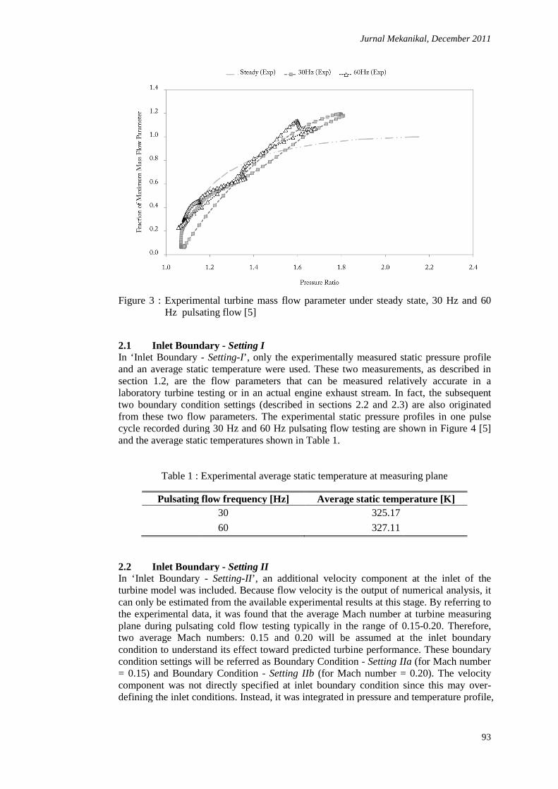
Figure 3 : Experimental turbine mass flow parameter under steady state, 30 Hz and 60 Hz pulsating flow

2.1 Inlet Boundary In ‘Inlet Boundary -and an average static temperature were used. These two measurements, as described in section 1.2, are the flow parameters that can be measured relatively accurate in a laboratory turbine testing otwo boundary condition settings (described in sections 2.2 from these two flow parameters. The experimental static pressure profiles in one pulse cycle recorded during 30 Hz and the average static temperatures shown in Tab

Table 1 : Experimental average static temperature at measuring plane

Pulsating flow frequency [Hz]

2.2 Inlet BoundaryIn ‘Inlet Boundary turbine model was included. Because flow velocity is the output of numerical analysis, it can only be estimated from the available experimental results at this stage.the experimental data, it was found that the average Mach number at turbine measuring plane during pulsating cold flowtwo average Mach numbers: 0.15 and 0.20 will be assumed at the inlet boundary condition to understand its effect toward predicted turbine performance. Thcondition settings will be referred as Boundary Condition= 0.15) and Boundary Conditioncomponent was not directly specified at inlet boundary condition since this may overdefining the inlet conditions. Instead, it was integrated in pressure and temperature profile,


Experimental turbine mass flow parameter under steady state, 30 Hz and 60 pulsating flow [5]

Inlet Boundary - Setting I - Setting-I’, only the experimentally measured static pressure profile

and an average static temperature were used. These two measurements, as described in section 1.2, are the flow parameters that can be measured relatively accurate in a laboratory turbine testing or in an actual engine exhaust stream. In fact, the subsequent two boundary condition settings (described in sections 2.2 and 2.3) are also originated from these two flow parameters. The experimental static pressure profiles in one pulse

ng 30 Hz and 60 Hz pulsating flow testing are shown in Figand the average static temperatures shown in Table 1.

: Experimental average static temperature at measuring plane

Pulsating flow frequency [Hz] Average static temperature [K]30 325.17

60 327.11

Inlet Boundary - Setting II - Setting-II’, an additional velocity component at the inlet of the included. Because flow velocity is the output of numerical analysis, it

can only be estimated from the available experimental results at this stage.the experimental data, it was found that the average Mach number at turbine measuring

e during pulsating cold flow testing typically in the range of 0.15two average Mach numbers: 0.15 and 0.20 will be assumed at the inlet boundary condition to understand its effect toward predicted turbine performance. Th

tion settings will be referred as Boundary Condition - Setting IIa= 0.15) and Boundary Condition - Setting IIb (for Mach number =component was not directly specified at inlet boundary condition since this may over

ining the inlet conditions. Instead, it was integrated in pressure and temperature profile,


93

Experimental turbine mass flow parameter under steady state, 30 Hz and 60

’, only the experimentally measured static pressure profile and an average static temperature were used. These two measurements, as described in section 1.2, are the flow parameters that can be measured relatively accurate in a

r in an actual engine exhaust stream. In fact, the subsequent 2.3) are also originated

from these two flow parameters. The experimental static pressure profiles in one pulse 60 Hz pulsating flow testing are shown in Figure 4 [5]

: Experimental average static temperature at measuring plane

Average static temperature [K]

an additional velocity component at the inlet of the included. Because flow velocity is the output of numerical analysis, it

can only be estimated from the available experimental results at this stage. By referring to the experimental data, it was found that the average Mach number at turbine measuring

of 0.15-0.20. Therefore, two average Mach numbers: 0.15 and 0.20 will be assumed at the inlet boundary condition to understand its effect toward predicted turbine performance. These boundary

Setting IIa (for Mach number = 0.20). The velocity

component was not directly specified at inlet boundary condition since this may over-ining the inlet conditions. Instead, it was integrated in pressure and temperature profile,


94

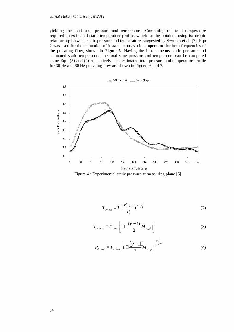
yielding the total state pressure and temperature. Computing the total temperature required an estimated static temperature profile, which can be obtained using iserelationship between 2 was used for the estimation of instantaneous static tethe pulsating flow, shown in Figestimated static temperature, the total state pressure and temperature can be computed using Eqn. (3) and (4) respectively. The estimated total pressure and temperature profile for 30 Hz and 60 Hz pulsating flow are shown in Fig

Figure 4

December 2011

yielding the total state pressure and temperature. Computing the total temperature required an estimated static temperature profile, which can be obtained using iserelationship between static pressure and temperature, suggested by Szymko et al. [7]. Eqn. 2 was used for the estimation of instantaneous static temperature for both frequencies the pulsating flow, shown in Figure 5. Having the instantaneous staestimated static temperature, the total state pressure and temperature can be computed

(4) respectively. The estimated total pressure and temperature profile 60 Hz pulsating flow are shown in Figures 6 and 7.

Figure 4 : Experimental static pressure at measuring plane [5]

γγ 1

)(−−

− =s

instssinsts P

PTT

−+= −− 22

)1(1

instinstsinst MTTγ

ο

( ) 1

22

11

−

−−

−+=γ

γ

ογ

instinstsinst MPP

yielding the total state pressure and temperature. Computing the total temperature required an estimated static temperature profile, which can be obtained using isentropic

static pressure and temperature, suggested by Szymko et al. [7]. Eqn. mperature for both frequencies of

5. Having the instantaneous static pressure and estimated static temperature, the total state pressure and temperature can be computed

(4) respectively. The estimated total pressure and temperature profile

: Experimental static pressure at measuring plane [5]

(2)

(3)

(4)

Figure 5

Figure 6


Figure 5 : Estimated static temperature at measuring plane

Figure 6 : Estimated total pressure at measuring plane


95

Estimated static temperature at measuring plane

: Estimated total pressure at measuring plane


96

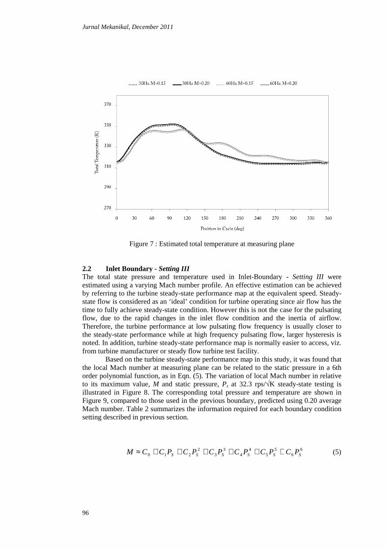
Figure 7 2.2 Inlet Boundary The total state pressure and temperature used in Inletestimated using a varying Mach number profile. An effective estimation can be achieved by referring to the turbine steadystate flow is considered as an ‘ideal’ condition for turbine operating sintime to fully achieve steadyflow, due to the rapid changes in the inlet flow condition and the inertia of airflow. Therefore, the turbine performance at low pulsating flowthe steady-state performance while at high frequency pulsating flow, larger hysteresis is noted. In addition, turbine steadyfrom turbine manufacturer or steady flow t Based on the turbine steadythe local Mach number at measuring plane can be related to the static pressure in a 6th order polynomial function, as in Eqto its maximum value, illustrated in FigureFigure 9, compared to those used in the previous boundary, predicted using 0.20 average Mach number. Tablesetting described in previous section.

M ≈

December 2011

Figure 7 : Estimated total temperature at measuring plane

Inlet Boundary - Setting III The total state pressure and temperature used in Inlet-Boundaryestimated using a varying Mach number profile. An effective estimation can be achieved by referring to the turbine steady-state performance map at the equivalent speed. Steadystate flow is considered as an ‘ideal’ condition for turbine operating sintime to fully achieve steady-state condition. However this is not the case for the pulsating flow, due to the rapid changes in the inlet flow condition and the inertia of airflow. Therefore, the turbine performance at low pulsating flow frequency is usually closer to

state performance while at high frequency pulsating flow, larger hysteresis is noted. In addition, turbine steady-state performance map is normally easier to access, viz. from turbine manufacturer or steady flow turbine test facility.

Based on the turbine steady-state performance map in this study, it was found that the local Mach number at measuring plane can be related to the static pressure in a 6th order polynomial function, as in Eqn. (5). The variation of local Mach number in relative to its maximum value, M and static pressure, Ps at 32.3 rps/√K steady

ure 8. The corresponding total pressure and temperature are shown in 9, compared to those used in the previous boundary, predicted using 0.20 average

le 2 summarizes the information required for each boundary condition setting described in previous section.

55

44

33

2210 SSSSS PCPCPCPCPCC ++++++≈

measuring plane

Boundary - Setting III were estimated using a varying Mach number profile. An effective estimation can be achieved

state performance map at the equivalent speed. Steady-state flow is considered as an ‘ideal’ condition for turbine operating since air flow has the

state condition. However this is not the case for the pulsating flow, due to the rapid changes in the inlet flow condition and the inertia of airflow.

frequency is usually closer to state performance while at high frequency pulsating flow, larger hysteresis is

state performance map is normally easier to access, viz.

state performance map in this study, it was found that the local Mach number at measuring plane can be related to the static pressure in a 6th

n of local Mach number in relative K steady-state testing is

8. The corresponding total pressure and temperature are shown in 9, compared to those used in the previous boundary, predicted using 0.20 average

2 summarizes the information required for each boundary condition

66 SPC+ (5)

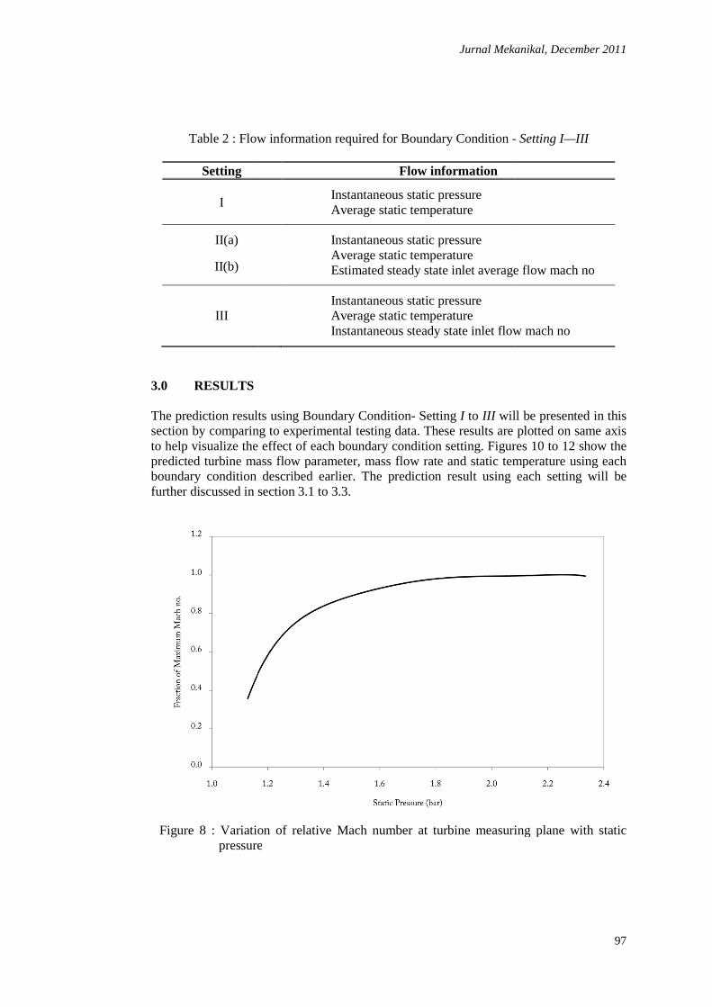
Table 2 : Flow information required for Boundary Condition

Setting

I

II(a)

II(b)

III

3.0 RESULTS The prediction results using Boundary Conditionsection by comparing to experimental testing data.to help visualize the effect of each boundary condition setting. predicted turbine mass flow parameter, mass flowboundary condition described earlier.further discussed in section 3.1 to 3.3.

Figure 8 : Variation of relative Mach number at turbine measuring plane with staticpressure


: Flow information required for Boundary Condition -

Flow information

Instantaneous static pressure Average static temperature

Instantaneous static pressure Average static temperature Estimated steady state inlet average flow mach no

Instantaneous static pressure Average static temperature Instantaneous steady state inlet flow mach no

The prediction results using Boundary Condition- Setting I to III will be presented in this section by comparing to experimental testing data. These results are plotted on same axis to help visualize the effect of each boundary condition setting. Figure

turbine mass flow parameter, mass flow rate and static temperature using each boundary condition described earlier. The prediction result using each setting will be further discussed in section 3.1 to 3.3.

Variation of relative Mach number at turbine measuring plane with staticpressure


97

- Setting I—III

state inlet average flow mach no

Instantaneous steady state inlet flow mach no

will be presented in this These results are plotted on same axis

ures 10 to 12 show the static temperature using each

result using each setting will be

Variation of relative Mach number at turbine measuring plane with static


98

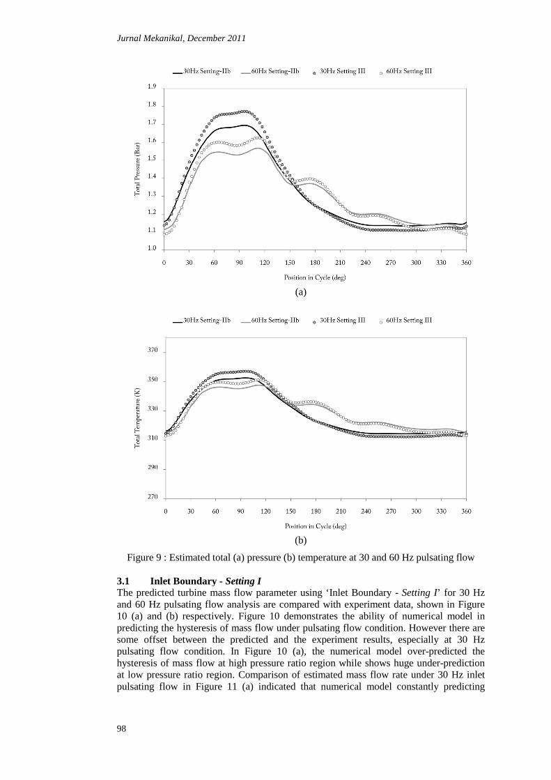
Figure 9 : Estimated total (a) pressure (b) temperature at 30 3.1 Inlet Boundary The predicted turbine mass flow parameter using ‘Inlet Boundaryand 60 Hz pulsating flow 10 (a) and (b) respectively. Figpredicting the hysteresis of mass flow under pulsating flow condition. However there are some offset between tpulsating flow condition. In Fighysteresis of mass flow at high pressure ratio region while shows huge underat low pressure ratio repulsating flow in Fig

December 2011

(a)

(b)

Estimated total (a) pressure (b) temperature at 30 and 60

Inlet Boundary - Setting I The predicted turbine mass flow parameter using ‘Inlet Boundary - and 60 Hz pulsating flow analysis are compared with experiment data, shown in Fig

(b) respectively. Figure 10 demonstrates the ability of numerical model in predicting the hysteresis of mass flow under pulsating flow condition. However there are some offset between the predicted and the experiment results, especially at 30 Hz pulsating flow condition. In Figure 10 (a), the numerical model overhysteresis of mass flow at high pressure ratio region while shows huge underat low pressure ratio region. Comparison of estimated mass flow rate under 30 Hz inlet pulsating flow in Figure 11 (a) indicated that numerical model constantly predicting

60 Hz pulsating flow

Setting I’ for 30 Hz analysis are compared with experiment data, shown in Figure

10 demonstrates the ability of numerical model in predicting the hysteresis of mass flow under pulsating flow condition. However there are

he predicted and the experiment results, especially at 30 Hz 10 (a), the numerical model over-predicted the

hysteresis of mass flow at high pressure ratio region while shows huge under-prediction gion. Comparison of estimated mass flow rate under 30 Hz inlet

11 (a) indicated that numerical model constantly predicting

higher mass flow rate than the experiment except in the region of 80°The numerical modillustrated in Figurescovered the actual operating range of the turbine. However the boundary setting was found to be very poor in temperature prediction. Due to only an average static temperature was specified the boundary eventually became a stagnant reservoir where only the pressure is altering while temperature remains unchanged. Theoretically, the input pressure and temperature in this case were the total state parameters since no velocity component was included.

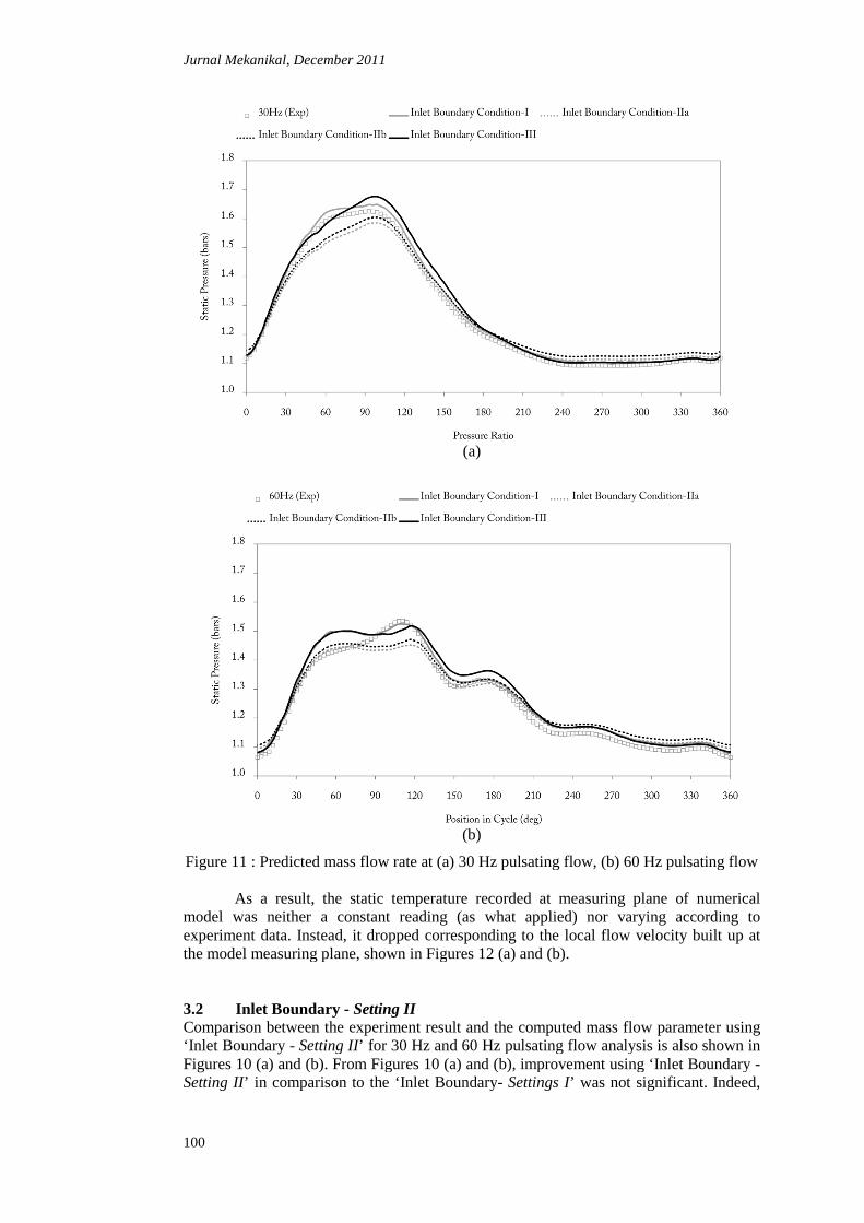
Figure 10 : Predicted mass flow parameter at (a) 30Hz pulsating flow, (b) 60Hz pulsating flow


higher mass flow rate than the experiment except in the region of 80°The numerical model performed much better during 60 Hz pulsating flow analysis,

s 10 (b) and 11 (b). The predicted mass flow parameter almost fully covered the actual operating range of the turbine. However the boundary setting was found to be very poor in temperature prediction. Due to only an average static temperature was specified at the turbine inlet, the inlet environment immediately prior to the boundary eventually became a stagnant reservoir where only the pressure is altering while temperature remains unchanged. Theoretically, the input pressure and temperature

e the total state parameters since no velocity component was included.

(a)

(b)

Predicted mass flow parameter at (a) 30Hz pulsating flow, (b) 60Hz pulsating


99

higher mass flow rate than the experiment except in the region of 80°-140° in pulse cycle. el performed much better during 60 Hz pulsating flow analysis, 10 (b) and 11 (b). The predicted mass flow parameter almost fully

covered the actual operating range of the turbine. However the boundary setting was found to be very poor in temperature prediction. Due to only an average static

at the turbine inlet, the inlet environment immediately prior to the boundary eventually became a stagnant reservoir where only the pressure is altering while temperature remains unchanged. Theoretically, the input pressure and temperature

e the total state parameters since no velocity component was included.

Predicted mass flow parameter at (a) 30Hz pulsating flow, (b) 60Hz pulsating


100

Figure 11 : Predicted mass flow rate at (a) 30 Hz pulsating

As a result, the static temperature recorded at measuring plane of numerical model was neither a constant reading (as what applied) nor varying according to experiment data. Instead, it dropped corresponding to the lthe model measuring plane, shown in Fig 3.2 Inlet Boundary Comparison between the experiment result and the computed mass flow parameter using ‘Inlet Boundary - Setting IIFigures 10 (a) and (b). From FigSetting II’ in comparison to the ‘Inlet Boundary

December 2011

(a)

(b)

Predicted mass flow rate at (a) 30 Hz pulsating flow, (b) 60 Hz pulsating flow

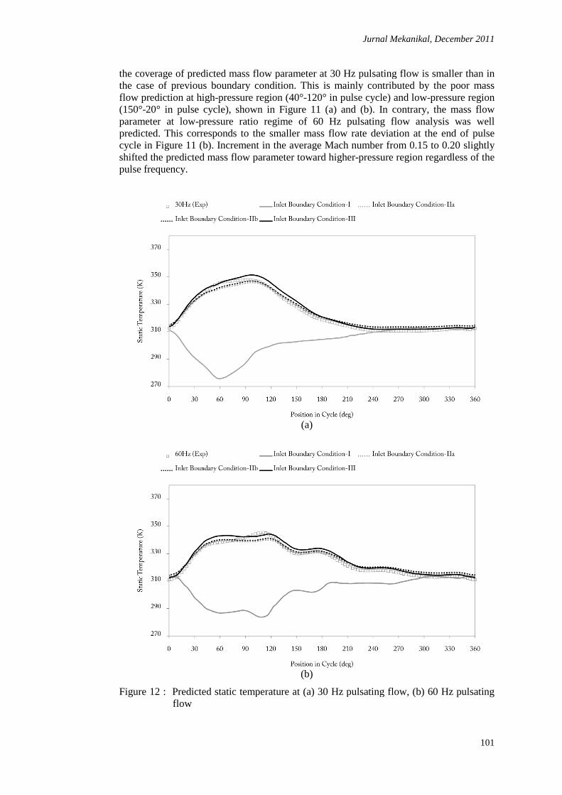
As a result, the static temperature recorded at measuring plane of numerical model was neither a constant reading (as what applied) nor varying according to experiment data. Instead, it dropped corresponding to the local flow velocity built up at the model measuring plane, shown in Figures 12 (a) and (b).

Inlet Boundary - Setting II Comparison between the experiment result and the computed mass flow parameter using

Setting II’ for 30 Hz and 60 Hz pulsating flow analys(b). From Figures 10 (a) and (b), improvement using ‘Inlet Boundary

in comparison to the ‘Inlet Boundary- Settings I’ was not significant.

flow, (b) 60 Hz pulsating flow

As a result, the static temperature recorded at measuring plane of numerical model was neither a constant reading (as what applied) nor varying according to

ocal flow velocity built up at

Comparison between the experiment result and the computed mass flow parameter using Hz pulsating flow analysis is also shown in

(b), improvement using ‘Inlet Boundary - was not significant. Indeed,

the coverage of predicted mass the case of previous boundary condition. This is mainly contributed by the poor mass flow prediction at high(150°-20° in pulse cyclparameter at low-pressure ratio regime of 60 Hz pulsating flow analysis was well predicted. This corresponds to the smaller mass flow rate deviation at the end of pulse cycle in Figure 11 (b). shifted the predicted mass flow parameter toward higherpulse frequency.

Figure 12 : Predicted flow


of predicted mass flow parameter at 30 Hz pulsating flow is smaller than in the case of previous boundary condition. This is mainly contributed by the poor mass flow prediction at high-pressure region (40°-120° in pulse cycle) and low

20° in pulse cycle), shown in Figure 11 (a) and (b). In contrary, the mass flow pressure ratio regime of 60 Hz pulsating flow analysis was well

predicted. This corresponds to the smaller mass flow rate deviation at the end of pulse 11 (b). Increment in the average Mach number from 0.15 to 0.20 slightly

shifted the predicted mass flow parameter toward higher-pressure region regardless of the

(a)

(b)

Predicted static temperature at (a) 30 Hz pulsating flow,


101

flow parameter at 30 Hz pulsating flow is smaller than in the case of previous boundary condition. This is mainly contributed by the poor mass

120° in pulse cycle) and low-pressure region (b). In contrary, the mass flow

pressure ratio regime of 60 Hz pulsating flow analysis was well predicted. This corresponds to the smaller mass flow rate deviation at the end of pulse

Increment in the average Mach number from 0.15 to 0.20 slightly pressure region regardless of the

static temperature at (a) 30 Hz pulsating flow, (b) 60 Hz pulsating


102

The underestimation of mass flow at high-pressure region is due to improper definition of total temperature at inlet boundary condition. In reality, the local Mach number is also in a pulse form, which leads to the profile seen in instantaneous mass flow rate. Due to the assumption of average local Mach number, the total temperature estimated was not correlate well with the actual total temperature at extremely high and low temperature region. This explained the deviation of mass flow rate found in Figure 11, where only mass flow rate correspond to intermediate temperature level was well matched. However, the variation trend of the static temperature at measuring plane for both frequency of pulsating flow analysis was correctly predicted using ‘Inlet Boundary-Setting II’. This is shown in Figures 12 (a) and (b). 3.3 Inlet Boundary - Setting III The comparison of predicted mass flow parameter using ‘Inlet Boundary - Setting III’ and experimental results are shown in Figure 10 (a) and (b). The predictions using this setting covered wider mass flow parameter and pressure ratio range than the previous setting. In comparison to the ‘Inlet Boundary - Setting I’ , prediction using ‘Inlet Boundary - Setting III ’ is closer to the experimental mass flow parameter hysteresis at high pressure region, under 30 Hz inlet pulse flow, while the mass flow parameter predicted at low pressure ratio range shows negligible changes. For 60 Hz pulsating flow analysis, prediction at low-pressure ratio regime showed good agreement with the experiment. While at higher pressure ratio, prediction result deviated marginally from experiment but still within acceptable range. Comparison of predicted instantaneous mass flow rate and static temperature with experiment results are shown in Figures 11(a) and (b) and 12 (a) and (b) respectively. The mass flow rate predicted is rather similar to those in the Setting II except the deviation at extreme high and low pressure region is much smaller. This improvement is corresponding to the refinement made in estimation of the inlet total state parameters. In terms of static temperature, prediction results are almost exactly as experiment. 4.0 SUMMARY OF FINDINGS Turbine performance prediction was carried out using three different settings of inlet boundary conditions. ‘Inlet Boundary - Setting III’ described in section 2.3 was found to deliver best prediction in term of static temperature, mass flow rate, mass flow parameter and pressure ratio amongst other settings. Turbine mass flow parameter predicted using ‘Inlet Boundary - Setting I’ explained in section 2.1 was found fairly similar to those using ‘Inlet Boundary - Setting III’, but gave very poor prediction in the static temperature. On the other hand, ‘Inlet Boundary - Setting II’ described in section 2.2, delivered satisfactory static temperature prediction but gave the worst mass flow parameter results amongst all other boundary condition settings.

From this series of studies, the inlet boundary condition setting for 1 dimensional turbine pulsating flow performance analysis under different circumstances can be summarized as below:

1. When only the instantaneous flow static pressure and average temperature are available, ‘Inlet Boundary - Setting I’ can be used strictly for turbine mass flow parameter prediction. However, this boundary setting does not provide correct static temperature prediction.

2. For static temperature prediction, ‘Inlet Boundary - Setting II’ can be used. However, mass flow rate and mass flow parameter prediction using this setting are less satisfactory.


103

3. In the case where turbine steady-state performance map is available, ‘Inlet Boundary - Setting III’ can be utilized for better turbine mass flow parameter as well as static temperature prediction.

4.1 Future work The available net power output of turbine is the one of the most important result in any turbine analysis, either for turbine designer or for engine-turbocharger matching application. Even though the boundary condition settings discussed in this paper showed acceptable flow performance prediction; these do not guarantee a good efficiency prediction. This is due to the current wave action code is specifically built for flow performance and wave action study, thus the efficiency calculation still rely on quasi-steady interpolation from steady state performance map. One of the effective yet simple ways of including turbine efficiency calculation is by appending a mean line model to the one-dimensional turbine model shown in this paper [14]. This method was proved capable of predicting the hysteresis of unsteady turbine efficiency and delivered close average value to experimental result. Future work should extend current model for power and efficiency calculation apart from the flow performance prediction.

ACKNOWLEDGEMENTS

The authors are thankful to Caterpillar Inc., Energy and Power Systems Research UK for permission to use the experimental data. The authors would also like to thank the Ministry of Higher Education and Universiti Teknologi Malaysia for Research University Grant VOT 01J49.

REFERENCES

1. Abidat, M., Hachemi, M., Hamidou, M.K., Baines, N.C., 1998. Prediction of the steady and non-steady flow performance of a highly loaded mixed flow turbine, Proceedings of the Institution of Mechanical Engineers; 212 (3), 173--184.

2. Ghassemi, S., Shirani, E. and Hajilouy-Benisi, A., 2005. Performance Prediction of Twin-Entry Turbocharger Turbines, Iranian Journal of Science and Technology, Transaction B, Engineering, 29 (B2), 145--155.

3. Romagnoli, A. and Martinez-Botas, R. F., 2011. Performance prediction of a nozzled and nozzleless mixed flow turbine in steady conditions, International Journal of Mechanical Sciences, 53, 557--574.

4. Serrano, J.R., Arnau, F.J., Dolz, V., Tiseira, A., Cervelló, C., 2008. A model of turbocharger radial turbines appropriate to be used in zero- and one-dimensional gas dynamic codes for internal combustion engines modeling, Energy Conversion and Management, 49 (12), 3729--3745.

5. Costall, A.W., McDavid, R.M., Martinez-Botas, R.F., and Baines, N.C., 2011. Pulse performance modeling of a twin entry turbocharger turbine under full and unequal admission, Journal of Turbomachinery, 133(2), 1005-1--9.

6. British Standards. BS EN ISO 5167-1:1997: Measurement of fluid flow by means of pressure differential devices, Part 1, 1997.

7. Szymko, S., Martinez-Botas, R.F. and Pullen, K.R., 2005. Experimental evaluation of turbocharger turbine performance under pulsating flow conditions, Proceedings of the ASME Turbo Expo 2005: Power for Land, Sea and Air, Paper no. GT 2005-68878.

8. Nyquist Rate. Last accessed 24.11.11; URL: http://en.wikipedia.org/wiki/Nyquist_rate.

9. RDP Electronics, 2001. Fast response from pressure transducer, CIP-Ultra pressure transducer. Last accessed 24.11.11; URL: http://source.theengineer.co.uk/measurement-quality-control-and-test/vision-sound-


104

and-vibration-testing/vision-and-colour-systems/fast-response-from-pressure-transducer/72755.article.

10. Sarnes, B., and Schrüfer, E., 2007. Determination of the time behavior of thermocouples for sensor speedup and medium supervision, Proc. Estonian Acad. Sci. Eng., 13 (4), 295--309.

11. Sieverding, C. H., Arts,T., Denos,R. and Brouckaert, J.-F., 2000. Measurement techniques for unsteady flows in turbomachines, Experiments in Fluid, 28 (4), 285-321.

12. Manuel, A. A. M. and Viviana, S. F., 2010. Gas mass-flow meters: Principles and applications, Flow Measurement and Instrumentation, 21 (2), 143--149.

13. Syzmko, S., Martinez-Botas, R.F., Pullen, K.R., McGlashan, N.R. and Chen, H., 2002. A High-Speed Permanent Magnet Eddy-Current Dynamometer for Turbocharger Research, Proceedings. of IMechE 7th International Conference on turbochargers and turbocharging, C602/026/2002, 213--224.

14. Chiong M.S., Rajoo, S., Romagnoli, A. and Martinez-Botas, R. F., 2011. Single entry mixed flow turbine performance prediction with 1-D gas dynamic code coupled with mean line model, 10th International Gas Turbine Congress, IGTC2011-0158.

Nomenclature

A Area (m2) C Constant Cd Discharge coefficient f Frequency (Hz) M Mach number �� Mass flow rate (kg/s) P Pressure (Pa) T Temperature (K) v Velocity (m/s)

Greek letters � Orifice area ratio � Expansion ratio � Density (kg/m3) � Ratio of specific heat � Pulse period fraction

Subscript 0 Total state

inst Instantaneous orif orifice s Static state

Inlet Boundary Condition Study for ... - Jurnal...

Documents

Transcript of Inlet Boundary Condition Study for ... - Jurnal...