INITIAL MARGIN CALCULATION ON DERIVATIVE MARKETS SPAN METHOD® Derivatives... · The document might...

Initial Margin calculation on derivative markets: SPAN® method

LCH.Clearnet SA

INITIAL MARGIN CALCULATION ON DERIVATIVE MARKETS

SPAN® METHOD

Version: 2.1 Date: January 2012

Disclaimer

This document is solely intended as information for clearing members and others who are interested in the clearing process

operated by LCH.Clearnet. It is a commercial presentation of one of the service to be provided by LCH.Clearnet SA and not a

binding commercial offer.

Although all reasonable care has been taken in the preparation of this document LCH.Clearnet disclaims liability of the

information and for the uses to which it is put.

The document might be upgraded along the project implementation period.

Copyright

All the intellectual property rights of the technical presentation and the diagrams included in this document are vested in

LCH.Clearnet SA.

This work is issued in confidence for the purpose for which it is supplied. It must not be reproduced in whole or in part or used

for other purposes except with the consent in writing of LCH.Clearnet SA and then only on the condition that this notice is

included in any such reproduction. The information that is part of the document is solely for information purpose and is not to be

construed as technical specification.

CONTENTS


LCH.Clearnet SA 2/49

CONTENTS

FOREWORD ............................................................................................................................................ 4

INTRODUCTION ....................................................................................................................................... 5

CHAPTER I GENERAL OVERVIEW ..................................................................................................... 6

GENERAL DIAGRAM OF THE SPAN®

METHODOLOGY ................................................................................ 7

RISK ARRAYS, SCANNING RISK AND NET DELTA ..................................................................................... 8

INTER-MONTH (OR INTRA-COMMODITY) SPREAD CHARGE ......................................................................... 8

SPOT (DELIVERY) MONTH CHARGE ......................................................................................................... 9

INTER-COMMODITY SPREAD CREDIT ........................................................................................................ 9

SHORT OPTION MINIMUM ........................................................................................................................ 9

PERFORMANCE BOND AMOUNT ............................................................................................................... 9

CHAPTER II RISK ARRAY, SCANNING RISK AND NET DELTA..................................................... 11

RISK ARRAY ......................................................................................................................................... 12 Principle .......................................................................................................................................... 12 Risk Array calculation ..................................................................................................................... 12 Risk Array calculation parameters ................................................................................................. 12 Risk Array example ........................................................................................................................ 14

SCANNING RISK ................................................................................................................................... 15 Principle .......................................................................................................................................... 15 Scanning Risk amount calculation ................................................................................................. 15 Scanning Risk calculation and Active Scenario determination example ....................................... 16

CONCEPT OF NET DELTA ...................................................................................................................... 17 Principle .......................................................................................................................................... 17 Net Delta calculation ...................................................................................................................... 17 Net Delta example .......................................................................................................................... 18

CHAPTER III INTER-MONTH OR INTRA-COMMODITY SPREAD CHARGE ................................... 19

INTER-MONTH OR INTRA-COMMODITY SPREAD CHARGE ......................................................................... 20 Principle .......................................................................................................................................... 20 Inter-month Spread charge calculation .......................................................................................... 20 Inter-month Spread charge example .............................................................................................. 21

CHAPTER IV SPOT (DELIVERY) MONTH CHARGE ........................................................................ 26

SPOT (DELIVERY) MONTH CHARGE ....................................................................................................... 27 Principle .......................................................................................................................................... 27 Spot Month charge calculation ....................................................................................................... 27 Spot Month charge example .......................................................................................................... 28

CHAPTER V INTER-COMMODITY SPREAD CREDIT ....................................................................... 29

INTER-COMMODITY SPREAD CREDIT ...................................................................................................... 30 Principle .......................................................................................................................................... 30 Inter-commodity Spread credit calculation ..................................................................................... 30 Inter-commodity Spread credit example ........................................................................................ 33

CHAPTER VI SHORT OPTION MINIMUM (SOM) .............................................................................. 38

SHORT OPTION MINIMUM (SOM) .......................................................................................................... 39 Principle .......................................................................................................................................... 39 Short Option Minimum calculation ................................................................................................. 39 Short Option Minimum example ..................................................................................................... 39

CONTENTS



CHAPTER VII PERFORMANCE BOND AMOUNT ............................................................................. 40

PERFORMANCE BOND AMOUNT ............................................................................................................. 41 Principle .......................................................................................................................................... 41 Performance Bond Amount calculation .......................................................................................... 41 Performance Bond amount example .............................................................................................. 42

CHAPTER VIII EQUITY CROSS-MARGINING MANAGEMENT ........................................................ 44

PERFORMING CALCULATIONS WITH CROSS-MARGINING POSITIONS ........................................................ 45 Principle .......................................................................................................................................... 45 Cross-Margining calculations ......................................................................................................... 45 Cross-Margining example .............................................................................................................. 46

CONCEPT OF PERFORMANCE BOND GROUP .......................................................................................... 47 Principle .......................................................................................................................................... 47 performance bond group calculations ............................................................................................ 47 Performance Bond Group example ................................................................................................ 49

FOREWORD



FOREWORD The parameters and the contracts used in the examples or the texts of this document are given for information. Indeed, LCH.Clearnet SA regularly reviews these parameters according to the markets conditions. These parameters are available on the LCH.Clearnet website at the following address:

www.lchclearnet.com For all questions about margin calculation methods, please contact:

[email protected]

SPAN and Standard Portfolio Analysis of Risk are registered trademarks of the Chicago Mercantile

Exchange. Chicago Mercantile Exchange assumes no liability in connection with the use of SPAN by any person or entity. A Glossary and Option Pricing formula documents in order to complete this document are also available on the website.

http://www.lchclearnet.com/

INTRODUCTION



INTRODUCTION The present brochure describes the calculation method for the initial margins required for the regulated derivatives market cleared by LCH.Clearnet SA. The initial margin required by LCH.Clearnet SA from its members is to cover potential losses following the liquidation of a failing member’s positions. LCH.Clearnet SA's members can apply the same methodology to cover risk on open positions from their clients. The calculation method of this initial margin aims at ensuring market safety while reducing the costs for financing operations on the market. Initial margin represents one of the three elements composing the financial cover call. These three elements are defined as follows:

PAYMENT OF VARIATION MARGINS ON FUTURES CONTRACTS, IMMEDIATE PAYMENT OF THE PREMIUM BY THE OPTION BUYER TO THE SELLER, COVERAGE OF A PERFORMANCE BOND AMOUNT ON THE OPEN POSITIONS.

The SPAN method is based on the estimation of the overall risk exposure of a portfolio and combines options and futures positions for calculation purposes. Initial margin therefore represents the most unfavourable liquidation value of a portfolio according to several scenarios representing adverse changes in market conditions. This data is stored in risk arrays, which are specific to each contract and updated on a daily basis. The scenarios used by SPAN

® notably consider the following events:

POSSIBLE VARIATION OF UNDERLYING PRICE POSSIBLE VARIATION OF UNDERLYING VOLATILITY IMPACT OF TIME DECAY ON OPTION VALUE

To estimate these scenarios, SPAN

® uses three complex option pricing models that take into account

parameters representing different events described previously:

THE BLACK 76 MODEL THE COX ROSS RUBINSTEIN MODEL THE GARMAN AND KOHLHAGEN MODEL

Option evaluation is executed by LCH.Clearnet SA (except for settlement prices and implied volatilities which are received from market), recorded and transmitted to members via risk arrays, thus avoiding any discrepancies in the calculations between LCH.Clearnet SA and other users of the method. For these calculations, LCH.Clearnet SA sets the value of all parameters used to calculate the initial margin.

GENERAL OVERVIEW



CHAPTER I

GENERAL OVERVIEW

GENERAL OVERVIEW



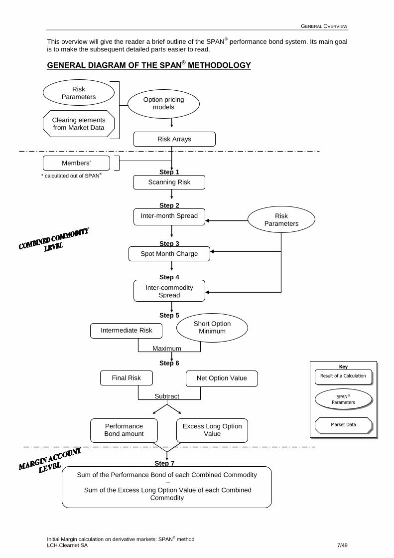
This overview will give the reader a brief outline of the SPAN

® performance bond system. Its main goal

is to make the subsequent detailed parts easier to read.

GENERAL DIAGRAM OF THE SPAN® METHODOLOGY

Performance Bond amount

Excess Long Option Value

Sum of the Performance Bond of each Combined Commodity –

Sum of the Excess Long Option Value of each Combined Commodity

Clearing elements from Market Data

Risk Parameters

Key

Result of a Calculation

SPAN®

Parameters

Market Data

Option pricing models

Risk Arrays

Spot Month Charge

Inter-commodity Spread

Risk Parameters

Scanning Risk

Step 1

Inter-month Spread

Step 2

Step 3

Step 4

Step 5

Step 6

Maximum

Final Risk Net Option Value

Step 7

Subtract

Short Option Minimum Intermediate Risk

Members' Positions

*

* calculated out of SPAN®

GENERAL OVERVIEW



The SPAN

® method makes a uniform evaluation of all products that have the same underlying

instrument thus taking an overall view of the portfolio composed of options and futures contracts. It considers not only Futures contracts and options on Futures contracts but also other types of options (equity options, currency options…).

RISK ARRAYS, SCANNING RISK AND NET DELTA The SPAN

® method is based on the estimation of the balance liquidation value of a portfolio according

to several scenarios anticipating the market’s evolution. This data is stored in Risk Arrays that are specific to each contract, and updated on a daily basis (see SPAN

® file description available on our

website). The scenarios used by SPAN

® consider the following:

Possible variation of underlying price, Possible variation of underlying volatility, Impact of time on option price.

All these factors have an impact on the value of the portfolio. Through these scenarios and using positions of the portfolio, SPAN

® determines the maximum loss sustained by this portfolio from one

market day to the next. This is the Scanning Risk. SPAN

® considers a total of 16 risk scenarios by using a scanning range, or fluctuation range of the

underlying instrument price and a volatility range defined for each Combined Commodity.

As can be seen on the diagram above, the basic concept used for risk calculation is the Combined Commodity. This is a set of contracts having the same underlying instrument. The

SPAN® method calculates the hedge using this concept.

The risk arrays integrate seven price variation possibilities:

No variation, Price increase or decrease corresponding to 1/3 of the scan range, Price increase or decrease corresponding to 2/3 of the scan range, Price increase or decrease corresponding to 3/3 of the scan range.

For each of these price changes, an upward or downward variation in volatility is also considered. Short option positions that are highly out of the money near expiration represent a specific problem; should the underlying instrument vary sharply, these positions could then be in the money. SPAN

®

includes two scenarios to consider this risk, one for the fall in the underlying price, the other for a rise in price corresponding to two scanning ranges. However, only a fraction of the total loss thus calculated is considered in the risk arrays. SPAN

® uses option’s delta information to determine Net delta positions. Net delta positions are the

"equivalent delta’s positions" and serve to form spreads.

INTER-MONTH (OR INTRA-COMMODITY) SPREAD CHARGE SPAN

® also takes into account reductions in risk due to the presence of opposite positions on different

months within the same Combined Commodity. The use of risk arrays implicitly assumes that price changes across months of a Combined Commodity are perfectly correlated, but this is not generally so.

GENERAL OVERVIEW



In order to correct this aspect, SPAN® proceeds as follows:

The net delta for each month1 for which a position is held is considered. Long net deltas are offset with

short net deltas. The highest number of possible spreads is formed. This number is then multiplied by the charge for each spread as specified by the clearing-house. The result is added to the amount calculated from the risk arrays (or “scanning risk”).

SPOT (DELIVERY) MONTH CHARGE In the case of deliverable contracts (Commodity futures) and Index Derivatives (CAC40, AEX, BEL 20, PSI 20 Future contracts), additional risk may arise when the delivery date is close. In order to consider this risk, SPAN

® adds two type of charges:

On spread positions including one delivery month, On straight positions for the delivery month.

INTER-COMMODITY SPREAD CREDIT For distinct contracts with correlated underlying instruments (CAC 40 Future, AEX and BEL 20 for example) or same underlying instrument (equity option Total-Fina Elf which is multi-listed: FP in Paris, TOT in Brussels), the price variations may be correlated. Therefore, opposite positions in two different combined commodities can lead to a reduction in the global risk of the position. A decrease in the performance bond requirement is therefore calculated. A priority table is supplied for this purpose as well. For these spreads, SPAN

® generates a credit expressed as a percentage of the performance

bond amount called for the Combined Commodity.

SHORT OPTION MINIMUM In the event of a sharp variation of the underlying instrument price, short option positions can lead to considerable losses. SPAN

® therefore includes an additional step: It calculates a minimum amount (named also "Short

Option Minimum") called for short positions in each Combined Commodity. This amount will be called if it is higher than the result obtained in the previous steps (see diagram).

PERFORMANCE BOND AMOUNT AT COMBINED COMMODITY LEVEL The Performance Bond amount required for a given Combined Commodity is the result of the calculations in the steps described above and formalised as followed:

minimum option Short

credit spreaddity Intercommo

charge monthDelivery

charge month Inter

Risk Scanning

; Max Risk Final

The net option value

2 is deducted from this total risk amount, as the calculated performance bond

equals the net value of the portfolio plus the risk. If the result is positive, it is the performance bond called for the Combined Commodity. If the result is negative, it is the Excess Long Option Value. This Excess Long Option Value will be isolated and used for the final calculation of the performance bond in the portfolio.

1 For options, "Month" is always the underlying one's i.e. Future expiration month when it's an Option on Future and a default one (2064/12) when underlying product is not a derivatives product (indices, currency rate, equities,). 2 The amount comes from the difference between long and short option values.

GENERAL OVERVIEW



AT MARGIN ACCOUNT LEVEL The total Excess Long Option Value calculated for a Margin Account, made up of products from different Combined Commodities, can reduce the total Performance Bond amount called for all the Combined Commodities. The total amount therefore required at the level of the Margin Account comes from the Performance Bond amount of each Combined Commodity, to which we subtract the sum of the Excess Long Option Value. This amount can be positive or null: if the total Excess Long Option Value is greater than the sum of the performance bonds of each Combined Commodity, the result – negative – is ignored, and no amount is called. We may formalize the calculation of the performance bond as follows: We note:

ni1,i

AmountPB the performance bond amount calculated on the Combined Commodity i,

0i

AmountPB

ni1,i

ELOV the Excess Long Option Value calculated for the Combined Commodity i,

0i

ELOV

Therefore, the final requirement calculated at the level of Margin account is:

0;n

1i iELOV

n

1i i AmountPBMax AmountBond ePerformanc Final .

The Derivatives Clearing System makes a distinction when a portfolio is cross-margined, meaning includes equity positions with equity option positions in order to benefit margin offset: it introduces the notion of Margin Account Group that influences the final performance

bond calculation. See Chapter VIII for a brief description of this method.

RISK ARRAY, SCANNING RISK AND NET DELTA



CHAPTER II





RISK ARRAY

PRINCIPLE A Risk Array is a set of 16 scenarios defined for a particular contract specifying how a hypothetical single long position will loss or gain value if corresponding risk scenario occurs from the current situation day to the near future (generally next day).

RISK ARRAY CALCULATION Each Risk Array scenario represents losses or gains due to hypothetical market conditions:

the (underlying) price movement: upward(+) and downward(-) with corresponding Scan Range fraction (0, 1/3, 2/3, 3/3, or 2)

the (underlying) volatility movement: upward(+) and downward(-) with corresponding Scan Range fraction (0 or 1),

from the current day to the next business day (this number of calendar days is represented by the parameter called Look ahead time (set in the record type B in the

SPAN risk parameter file).

As each scenario does not have the same probability, each scenario could be weight: for certain scenario, only a fraction is retained (35% instead of 100%). A Scan Range is a fluctuation range of the underlying instrument price and volatility defined for each Combined Commodity

1. LCH.Clearnet SA fixes Underlying Price Scan Range (UPSR) and Volatility

Scan Range (VRS) also called Performance Bond margin parameters (\\LCH.Clearnet\Risk Management\SA\Risk Notices\Margin Parameters) in order to absorb potential losses to cover the liquidation of the portfolio in case of member default.

RISK ARRAY CALCULATION PARAMETERS

SPAN calculates 16 Risk Array scenarios.

RISK

SCENARIOS 1 2 3 4 5 6 7 8 9 10 11 12 13 14 15 16

UNDERLYING

PRICE

VARIATION (*) 0 0 1/3 1/3 -1/3 -1/3 2/3 2/3 -2/3 -2/3 1 1 -1 -1 2 -2

VOLATILITY

VARIATION (*) 1 -1 1 -1 1 -1 1 -1 1 -1 1 -1 1 -1 0 0

WEIGHT

FRACTION

TAKEN INTO

ACCOUNT

100% 100% 100% 100% 100% 100% 100% 100% 100% 100% 100% 100% 100% 100% 35% 35%

(*) Expressed in Scan Range.

1 A Combined Commodity gathers all contracts that have the same underlying instrument and are combined for

margining calculation. For example, the Combined Commodity FCE is a set of products having CAC 40 index as underlying: PXA, PXL and the linked Futures contract FCE.

http://www.lchclearnet.com/risk_management/sa/risk_notices/default.asp

http://www.lchclearnet.com/risk_management/sa/risk_notices/default.asp




Each Risk Array value is calculated as the current contract price less the theoretical contract price obtained for the corresponding scenario by using the valuation model. Risk Array values are in currency in which the specific contract is denominated. For each contract, a Risk Array is generated every day, for a single long position.

By convention, Risk Array values are given for a single long position1. Losses for long

positions are expressed as positive numbers, and gains as negative numbers.

The Clearing House provides Risk Arrays through SPAN risk parameter files (record type 81, 82 and 83).

1 Here "long" refers to purchase of Future, Put or Call contracts.




RISK ARRAY EXAMPLE Let consider the following contract:

Combined Commodity

Contract

Price

Code Type Strike Maturity month

CVF

FCE PXA Call 5300 04/ 2007 100 304.88

Parameters used for Risk Array calculation:

Underlying Price Scan Range (UPSR)

Volatility Scan Range (VSR)

Underlying price Settlement date Interest rate Implied volatility Date of valuation Pricing model

280 pi, i.e. 2 800€ 22% 5 389.85 20070420 3.9% 21% 20070315 Black-I

Risk Array results:

Product PXA 200704 C 5300.00 Scenario

Delta Imp. Vol Settl. CVF 1 2 3 4 5 6 7 8 9 10 11 12 13 14 15 16

Price Variation of the

underlying

Relative Value 0 0 1/3 1/3 - 1/3 - 1/3 2/3 2/3 - 2/3 - 2/3 1 1 -1 -1 2 -2

Absolute

Value 5389.85 5389.85 5483.18 5483.18 5296.52 5296.52 5576.52 5576.52 5203.18 5203.18 5669.85 5669.85 5109.85 5109.85 5949.85 4829.85

Volatility Variation

Relative Value 1 -1 1 -1 1 -1 1 -1 1 -1 1 -1 1 -1 0 0

Absolute

Value 25.62% 16.38% 25.62% 16.38% 25.62% 16.38% 25.62% 16.38% 25.62% 16.38% 25.62% 16.38% 25.62% 16.38% 21.00% 21.00%

Loss / Gain fraction taken into account 100% 100% 100% 100% 100% 100% 100% 100% 100% 100% 100% 100% 100% 100% 35% 35%

Risk array value (read in record 81, 82& 83)

-231.94 364.39 -825.85 -284.02 284.93 896.49 -1490.02 -1028.97 721.06 1302.94 -2215.06 -1846.18 1076.37 1588.3 -1599.39 645.26 0.611 0.21 196.4 10

For example, the scenario number 6 of Risk Array values given above is positive: 896.49€. This means that a long position on this option contract will experience a loss of 896.49€ over the next trading day, in the case where the price of the underlying goes down by one-third of the Underlying Price Scan Range and the volatility of that underlying price decreases by the full amount of the Volatility Scan Range.




SCANNING RISK

PRINCIPLE Risk Arrays give the theoretical future loss/gain of a derivatives contract for the 16 hypothetical market scenarios. To evaluate the portfolio risk, SPAN

® calculates first of all the Scanning Risk at Combined

Commodity level. For each Combined Commodity in the portfolio, Scanning Risk is a global worst-case scenario along with the future price assumptions defined for the 16 scenarios of Risk Arrays.

SCANNING RISK AMOUNT CALCULATION For a Combined Commodity:

1. Multiply each contract positions quantity by each of the 16 Risk Array(s) value of the

corresponding contract sequence. 2. Add up these results by scenario to obtain 16 scenarios amount for the Combined

Commodity. 3. Select the largest amount(worst-case) within the 16 scenarios for the Combined

Commodity. This amount is called the Scanning Risk. The number of the Risk Arrays scenario that gives the largest amount(worst-case scenario) for the Combined Commodity is called the Active Scenario. If two scenarios have the same figure, the one with the lowest scenario number is the Active Scenario (for instance, if scenarios 11 and 15 give the same results, scenario 11 will be defined as the Active Scenario).

In case of the 16 Scanning Risk totals are negative (e.g. all corresponding to a gain) or zero (no risk), the Scanning Risk amount is set to zero.

In that particular case, the Active Scenario is set to the "less gain scenario".

In this first step of calculating Scanning Risk, the same Underlying Price and Volatility Scan Range (UPSR and VSR) are applied to all contracts belonging to the same Combined Commodity, irrespective of their maturity or specificities. As this is rarely the case in reality, SPAN

® method

integrates other calculation steps to ensure greater precision in calculating portfolio risks. Those steps are developed in the following Chapters. ROUND-UP RULES Scanning Risk is rounded to two decimals.




SCANNING RISK CALCULATION AND ACTIVE SCENARIO DETERMINATION EXAMPLE Case 1: Considering the following portfolio:

Combined Commodity

Contract

Price Net Quantity Code Type Strike Maturity month

Underlying Maturity month

CVF

FCE PXA Call 5300 04/2007 12/2064 10 196.40 4

Product Scenarios Delta Imp Vol Settl CVF

PF Contract Qty 1 2 3 4 5 6 7 8 9 10 11 12 13 14 15 16

PXA

200704 C

5300.00

1 -231.94 364.39 -825.85 -284.02 284.93 896.49 -1490.02 -1028.97 721.06 1302.94 -2215.6 -1846.18 1076.37 1588.3 -1599.39 645.26 0.6108 0,2 196,4 10

4 -927.76 1 457.56 -3 303.40 -1 136.08 1 139.72 3 585.96 -5 960.08 -4 115.88 2 884.24 5 211.76 -8 862.40 -7 384.72 4 305.48 6 353.20 -6 397.56 2 581.04 2.4432

Total BFCC : FCE -927.76 1 457.56 -3 303.40 -1 136.08 1 139.72 3 585.96 -5 960.08 -4 115.88 2 884.24 5 211.76 -8 862.40 -7 384.72 4 305.48 6 353.20 -6 397.56 2 581.04 10

Scanning Risk amount is 6 353.20€ (maximum loss for this portfolio). The Active Scenario is the scenario 14. Case 2: Considering the following portfolio:

Combined Commodity

Contract

Price Net Quantity

Code Type Strike Maturity month Underlying

Maturity month CVF

AEX FTI Futures 12/ 2007 12/ 2007 200 482.95 -2

AEX AEX Put 500 03/ 2007 12/ 2064 100 17.25 -3

Product Scenario

Delta Imp Vol

Settl CVF PF Contract Qty 1 2 3 4 5 6 7 8 9 10 11 12 13 14 15 16

FTI 200712 1 0.00 0.00 -1 600.00 -1 600.00 1 600.00 1 600.00 -3 200.00 -3 200.00 3 200.00 3 200.00 -4 800.00 -4 800.00 4 800.00 4 800.00 -3 360.00 3 360.00 1.0000 482,95

200 -2 0.00 0.00 3 200.00 3 200.00 -3 200.00 -3 200.00 6 400.00 6 400.00 -6 400.00 -6 400.00 9 600.00 9 600.00 -9 600.00 -9 600.00 6 720.00 -6 720.00 -2.0000

AEX 200703

P 500,00

1 63.61 64.17 842.09 862.92 -735.75 -735.74 1 447.48 1 545.01 -1 535.66 -1 535.66 1 689.41 1 721.69 -2 335.58 -2 335.58 603.75 -1 657.36 -0.9996 0.1885 17,25 100

-3 -190.83 -192.51 -2 526.27 -2 588.76 2 207.25 2 207.22 -4 342.44 -4 635.03 4 606.98 4 606.98 -5 068.23 -5 165.07 7 006.74 7 006.74 -1 811.25 4 972.08 2.9988

Total AEX BFCC scanning risk : -190.83 -192.51 673.73 611.24 -992.75 -992.78 2 057.56 1 764.97 -1 793.02 -1 793.02 4 531.77 4 434.93 -2 593.26 -2 593.26 4 908.75 -1 747.92 0.9988

Scanning Risk amount is 4 908.75€ (maximum loss for this portfolio). The Active Scenario is the scenario 15.




CONCEPT OF NET DELTA

PRINCIPLE Scanning Risk process is based on an overall estimation, i.e. futures and options positions are processed similarly, irrespective of expiry and correlation between instruments. So, SPAN

® margin methodology uses option’s delta to form spreads in order to consider in the

Initial Margin calculation:

Inter month spreads charge (spreads between maturity months),

Delivery month charge (or Spot month charge),

Credit for Inter-commodity spreads (spreads between Combined Commodities), which are not taken into account in the Scanning Risk process. The SPAN

® margin methodology uses delta value information to determine what would be the

“equivalent delta’s positions" in terms of underlying instrument of the position held in derivatives instruments. Option’s delta is calculated with settlement price and implied volatility of the clearing day. (See appendix's documents for option’s delta formula). By convention, unitary option’s delta is given for a long position. For call contracts, they are valued between 0 and 1, and on put contracts, between –1 and 0. By definition, delta for Futures contracts is always 1. SPAN

® risk parameter file includes with Risk Arrays data, the option’s delta value for each

contract in the record type 83. It is also called Composite Delta.

NET DELTA CALCULATION The "equivalent delta's positions" is so called Net Delta. For calculating Net Delta Per Month, SPAN

® considers the maturity month of the underlying contract which can differ from the one of

the option contract itself. For equities and index options, SPAN

® considers the underlying asset maturity month as a far

future month, actually December 2064. For Futures contract, as there is no underlying product, the maturity month used is the one of the contract itself. For a Combined Commodity:

1. Multiply each contracts positions quantity by the contract option’s delta value and by the Delta Scaling Factor to obtain "equivalent delta's positions" or Net Delta per contract.

2. Sum up "equivalent delta's positions" by underlying maturity month to obtain Net Delta Per Month.

As some product with different nominal value belong to the same Combined Commodities SPAN

®

uses a Delta Scaling Factor to weight position in order to take into account this difference of size. If the nominal value is not different in for products belonging to the same Combined Commodity, the Delta Scaling Factor is set to 1.

The Delta Scaling Factor is provided in the record B of the SPAN risk parameter file. ROUND-UP RULES Net Delta is rounded to the fourth decimal number.




NET DELTA EXAMPLE

Case 1: Considering the following portfolio with index futures and options:

Combined Commodity

Product Contract

Price Net Quantity

Delta



CVF

AEX FTI Futures 03/ 2007 03/ 2007 200 483.55 9 1

AEX FTI Futures 04/ 2007 04/ 2007 200 483.90 -3 1

AEX FTI Futures 12/ 2007 12/ 2007 200 482.95 -2 1

AEX AEX Put 500 03/ 2007 12/ 2064 100 17.25 -3 -0.9996

AEX AEX Put 530 05/ 2007 12/ 2064 100 51.30 4 -0.9338

AEX AEX Call 360 12/ 2007 12/ 2064 100 121.55 5 0.9093

Net Delta per Month calculation: AEX

Month Position Delta Delta Scaling factor Net delta per month

Total Month 03/2007 6 1.0000 2 9 1.0000 2 = 18.0000

Total Month 03/2007 -3 1.0000 2 -3 1.0000 2 = -6.0000

Total Month 12/2007 -2 1.0000 2 -2 1.0000 2 = -4.0000

Month 12/2064 Month 12/2064 Month 12/2064

Total Month 12/2064

-3 4 5

-0.9996 -0.9338 0.9093

1 1 1

(-3 (-0.9996) 1)

+ (4 - 0.9338 1)

+ (5*0.9093 1) =3.8101

According to the general principle of Net Delta calculation described before, the required contract month kept for option contract is the month of the underlying asset and not the option contract month itself. As a matter of fact, all option contracts are gathered in their underlying month, which is December 2064.

Case 2: Considering the following portfolio with commodity futures and options on commodity futures:

Combined Commodity

Product Contract

Price Net Quantity

Delta



CVF

EBM OBM Put 150.00 05/ 2007 05/ 2007 50 1.79 5 -0.3714

EBM EMB Futures 11/ 2007 11/ 2007 50 136.50 -5 1.0000

EBM OBM Call 137.00 11/ 2007 11/ 2007 50 3.31 14 0.5000

EBM EMB Futures 03/ 2008 03/ 2008 50 139.00 5 1.0000

EBM OBM Call 139.00 03/ 2008 03/ 2008 50 9.75 -14 0.5159

Month Position Delta Scaling factor Net delta per Month

Total Month 05/2007 +5 -0.3714 1 5 -0.3714 1 = -1.8570

Month 11/2007 Month 11/2007

Total Month 11/2007

-5 +14

+1.0000 +0.5000

1 1

(-5 1.0000 1)

+(+14x0.5000 1) = 2

Month 03/2008 Month 03/2008

Total Month 03/2008

+5 -14

+1.0000 +0.5159

1 1

(+5 1.0000 1)

+(-14 0.5159 1) = -2.2226

In this example, the option’s underlying is a Futures contract. Therefore, the underlying maturity month is the Futures contract maturity month.

INTER-MONTH OR INTRA-COMMODITY SPREAD CHARGE



CHAPTER III






PRINCIPLE The basic hypothesis used for calculating Scanning Risk is that underlying instruments' prices for the various maturity months are perfectly correlated. Based on this hypothesis, the risk relative to a long position expressed in Net Delta (called long Net Delta) for a given month is neutralized by a short position expressed in Net Delta (or short Net Delta) for another month in the Scanning Risk calculation. However, the underlying instruments' prices, from a maturity month to another, are not perfectly correlated. Gains on a maturity month do not totally offset losses on another, thus giving rise to an Inter-month risk. SPAN

® therefore calculates a margin charge relative to the Inter-month Spread risk in order to

cover it. This margin is called Inter-month Spread charge or Intra-commodity Spread charge (because it is calculated within the Combined Commodity). In this document, the name used is Inter-month Spread charge.

INTER-MONTH SPREAD CHARGE CALCULATION For each Combined Commodity and each contract in the portfolio, SPAN

® calculates the Net

Delta1. Then, using the Inter-month Spreads charge parameters, it forms Inter-month Spreads

between long and short Net Delta gathered by several maturity month (Level2 or Tier) and applies

a charge rate to each spreads formed. For a Combined Commodity:

1. Sum up long Net Delta per Month3 in one hand and short Net Delta per Month in other

hand according to the Level defined in parameter table to obtain long (positive) Net Delta and short (negative) Net Delta per Level.

2. Following defined priority order from the parameter table, determine the number of Inter-month Spreads: The number of Inter-month Spreads is determined by comparing the long Net Delta

per Level and the short Net Delta per Level divided by the Delta per Spread Ratio for each leg of the priority and by selecting the smallest absolute value.

The spreads are determined following a strict priority order. Net Delta positions not consumed in prior priority are kept for the next priorities spread until the complete use of the Net Delta positions according to defined priorities.

3. Calculate the charge amount for Inter-month Spreads of each priority by multiplying the number of determined spreads by the charge rate.

4. Sum up Inter-month Spreads charge of all priorities to obtain the total Inter-month Spreads charge amount of the Combined Commodity.

Two margin parameters tables are provided for Inter-month Spread charge calculation per Combined Commodity:

One is the "Levels" table in which you can find the way to gather per Level the Net Delta per Month for determining the spreads. These Levels are determined by LCH.Clearnet SA for each Combined Commodity concerned by Inter-month Spread Charge as well as Spot Month Charge (see Chapter IV). A Level gathers several maturity months together. A maturity month corresponds to a maturity month number. Maturity month numbers are the open tradable chronological maturity months of the underlying products of the contracts belonging to the Combined Commodity.

1 See definition in the previous chapter.

2 Term Level is used in Margin parameters document and Tier is used in SPAN

® risk parameter file description document. In this

document will use the term Level. 3 See definition of Net Delta Per Month in previous chapter.




The other one is the "Spreads rules and charge amounts" table in which you can find the way to process and calculate Inter-month Spread charge: Spread priority order for each Combined Commodity, Number of legs (usually two). Each Leg consists in three fields:

- Level defined in the "Levels" table above. - Delta per Spread Ratio indicates Net Delta per Level to use for determining the

spreads. - Delta per Spread Ratio of n amount means n amount of Net Delta can form one

spread for the concerned leg. Leg Side or Market Side indicator1 (A or B) is

related to the sign of the Net Delta (long [positive] or short [negative]). If Leg Sides are opposite (Leg1=A(B) and Leg2=B(A)), then Net Delta must have opposite sign for determining the spread (If B is long then A is short and vice versa). If Leg Sides are the same (Leg1=A(B) and Leg2=A(B)), then Net Delta must have the same sign for determining the spread (If A(B) is Short then the other Leg Side must be Short for forming spreads and vice versa).

These parameters are specified in the margin parameters tables document and in the SPAN

® risk

parameter file in records type 3 and C.

ROUND-UP RULES The Inter-month Spread charge amounts are rounded to two decimals.

INTER-MONTH SPREAD CHARGE EXAMPLE

MARGINS PARAMETERS TABLES FOR INTER-MONTH SPREAD CHARGE Table of Levels

Combined Commodity

Level Month date

AEX

L1 1-2 (Futures)

L2 3-4-5-6 (Futures)

L3 All options

The maturity month of the underlying product is the maturity month of the contract itself when the contract is a Future and the maturity month of underlying asset for options. When the contract is an option on Physicals (like Index, Currency options) or option on Equity, maturity month of the underlying is considered as a far future month, actually December 2064. When the contract is an option on Futures (like Commodities options), maturity month of the underlying is the maturity of the Futures. Considering this definition of the maturity month, Levels in the table above correspond to:

LEVEL L1 gathered future contracts from first maturity month to second maturity month. LEVEL L2 gathered from third maturity month to sixth. LEVEL L3 gathered all option contracts.

1 Term Leg Side is used in Margin parameters document and Market Side is used in SPAN® risk parameter file description document. In this document will use the term Leg Side.




Table of Spread rules and charge amounts

Combined Commodity Priority

Leg 1 Leg 2

Additional charge Delta per

Spread ratio

Side of the leg

Level

Delta per

Spread ratio

Side of the leg

Level

Index Derivatives

AEX

1 1 A L1 1 B L1 € 50 i.e. 0.25 ip1

2 1 A L2 1 B L2 € 690 i.e. 3.45 ip

3 1 A L1 1 B L2 € 690 i.e. 3.45 ip

4 1 A L1 1 B L3 € 500 i.e. 2.5 ip

Spread for Priority n°1 is first formed if positions allow it, within the limits of the required Net Delta. If unused Net Delta remain after the first Priority spreads have been formed, Spreading for Priority n°2 will be formed, and so on. INTER-MONTH SPREADS CHARGE CALCULATION Considering the following portfolio on business date March, 15

th 2007:

Combined Commodity

Product Contract

Price Net

Quantity Code Type Strike

Maturity month


CVF

AEX AEX Call 360 12/ 2007 12/ 2064 100 121.55 5

AEX AEX Put 530 05/ 2007 12/ 2064 100 51.30 4

AEX AEX Put 500 03/ 2007 12/ 2064 100 17.25 -3

AEX FTI Futures 03/ 2007 03/ 2007 200 483.55 9

AEX FTI Futures 04/ 2007 04/ 2007 200 483.90 -3

AEX FTI Futures 12/ 2007 12/ 2007 200 482.95 -2

At Combined Commodity level, for AEX Combined Commodity,

Calculating long (positive) and short (negative) Net Delta per Level:


Total Month 03/2007 9 1.0000 2 9 1.0000 2 = 18.0000

Total Month 04/2007 -3 1.0000 2 -3 1.0000 2 = -6.0000

Total Month 12/2007 -2 1.0000 2 -2 1.0000 2 = -4.0000

Month 12/2064 Month 12/2064 Month 12/2064

Total Month 12/2064

-3 4 5

-0.9996 -0.9338 0.9093

1 1 1

(-3 (-0.9996) 1)

+ (4 - 0.9338 1)

+ (5 -0.9093 1) =

3.8101

The Net Delta per Month for each Level is: Level Month Month number Net Delta per Month

L1

03/2007 1 18.0000

04/2007 2 -6.0000

L2

05/2007 3 0.0000

06/2007 4 0.0000

09/2007 5 0.0000

12/2007 6 -4.0000

L3 12/2064 All others 3.8101

The total long (positive) and the total short (negative) Net Delta are gathered by Level.

1 Amount in euros is given relatively to a Futures contract. 0.25 ip * 200 (cvf of AEX Futures) = 50 €




Long delta Short delta

Level 1 18.0000 -6.0000

Level 2 0.0000 -4.0000

Level 3 3.8101 0.0000

Overall Level 21.8101 -10.000

Inter-month Spread charge for each priority: Considering the tables of Level and Spread rules and charge amount given above, determine how many spreads can be formed, following the priority rules defined for the AEX Combined Commodity: Inter-month Spread charge for priority 1:

Priority

Leg 1 Leg 2

Delta per Spread

ratio

Leg Side

Level Delta per Spread

ratio

Leg Side

Level

1 1 A L1 1 B L1

SPAN

® applies this priority at Level 1 versus Level 1 for Net Delta with opposite side (A,B) and

with a Delta per Spread ratio equals to 1 for both sides. If Leg1 side is Long [Positive](A) then Leg2 must be Short [Negative ](B) and vice versa. The number of Inter-month Spreads is determined by comparing the absolute value of the total long Net Delta to the absolute value of the total long Net Delta and by selecting the smallest absolute value. For Level 1, there are 18 long Net Delta and 6 short Net Delta. The number of possible spreads is equal to: Minimum(│+18.0000 / 1(Delta per Spread ratio for Leg 1)│ , │-6.0000 / 1(Delta per Spread ratio for Leg 2)│) = 6 => 6 spreads are formed. The Inter-month Spread charge for priority 1 is equal to: 6.0000 (spreads) x (0.25 x €100)(charge x cvf per spread) = 150.00 €. The entire stock of negative Net Delta is used for Level 1. 18.0000 – 6.0000 = 12.000 long Net Delta are left unused for Level 1. Unused Net Delta after priority 1 will be used for the next priorities:

Remaining Long delta Remaining Short delta

Level 1 18.0000-6.000=12.0000 -6.0000-(-6.0000)=0.0000

Level 2 0.0000 -4.0000

Level 3 3.8101 0.0000

Spread charge for priority 2:

Priority

Leg 1 Leg 2

Delta per Spread

ratio

Leg Side


ratio

Leg Side

Level

2 1 A L2 1 B L2

SPAN


with a Delta per Spread ratio equals to 1 for both sides. For Level 2, there are 0 long Net Delta and 4 short Net Delta. The number of possible spreads is equal to:




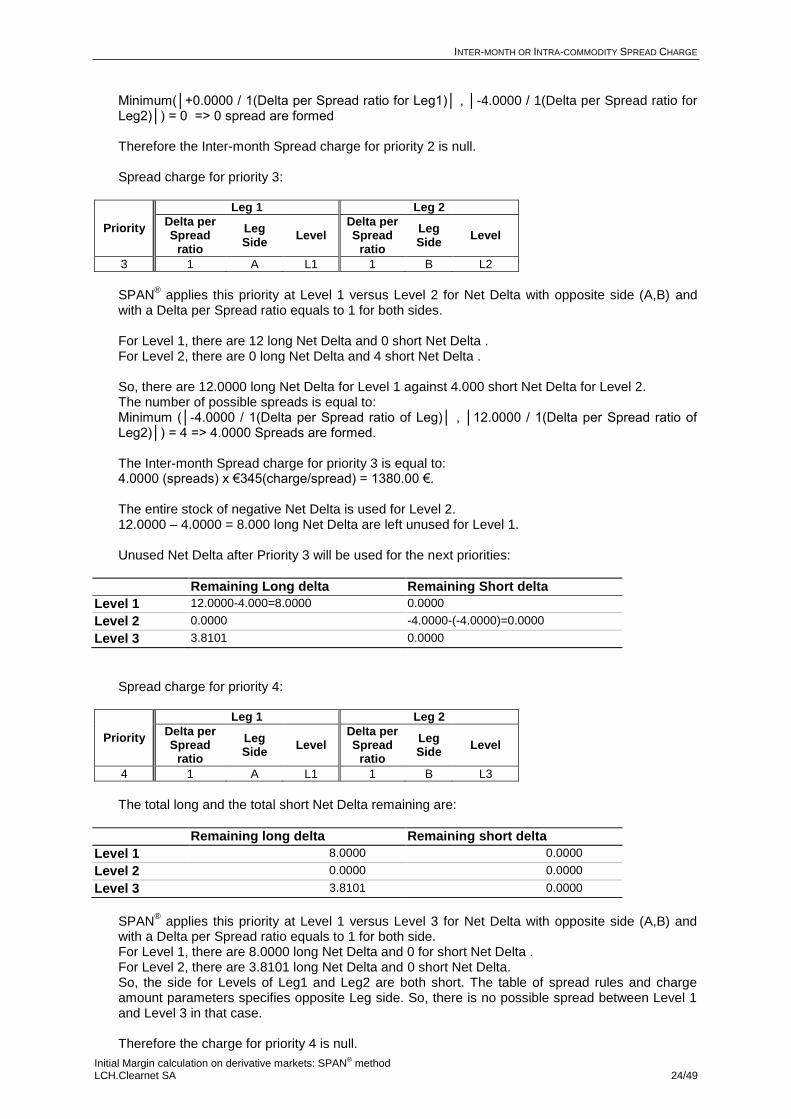
Minimum(│+0.0000 / 1(Delta per Spread ratio for Leg1)│ , │-4.0000 / 1(Delta per Spread ratio for Leg2)│) = 0 => 0 spread are formed Therefore the Inter-month Spread charge for priority 2 is null. Spread charge for priority 3:

Priority

Leg 1 Leg 2

Delta per Spread

ratio

Leg Side


ratio

Leg Side

Level

3 1 A L1 1 B L2

SPAN


with a Delta per Spread ratio equals to 1 for both sides. For Level 1, there are 12 long Net Delta and 0 short Net Delta . For Level 2, there are 0 long Net Delta and 4 short Net Delta . So, there are 12.0000 long Net Delta for Level 1 against 4.000 short Net Delta for Level 2. The number of possible spreads is equal to: Minimum (│-4.0000 / 1(Delta per Spread ratio of Leg)│ , │12.0000 / 1(Delta per Spread ratio of Leg2)│) = 4 => 4.0000 Spreads are formed. The Inter-month Spread charge for priority 3 is equal to: 4.0000 (spreads) x €345(charge/spread) = 1380.00 €. The entire stock of negative Net Delta is used for Level 2. 12.0000 – 4.0000 = 8.000 long Net Delta are left unused for Level 1. Unused Net Delta after Priority 3 will be used for the next priorities:

Remaining Long delta Remaining Short delta

Level 1 12.0000-4.000=8.0000 0.0000

Level 2 0.0000 -4.0000-(-4.0000)=0.0000

Level 3 3.8101 0.0000

Spread charge for priority 4:

Priority

Leg 1 Leg 2

Delta per Spread

ratio

Leg Side


ratio

Leg Side

Level

4 1 A L1 1 B L3

The total long and the total short Net Delta remaining are:

Remaining long delta Remaining short delta

Level 1 8.0000 0.0000

Level 2 0.0000 0.0000

Level 3 3.8101 0.0000

SPAN


with a Delta per Spread ratio equals to 1 for both side. For Level 1, there are 8.0000 long Net Delta and 0 for short Net Delta . For Level 2, there are 3.8101 long Net Delta and 0 short Net Delta. So, the side for Levels of Leg1 and Leg2 are both short. The table of spread rules and charge amount parameters specifies opposite Leg side. So, there is no possible spread between Level 1 and Level 3 in that case. Therefore the charge for priority 4 is null.




The unused Net Delta remains unchanged and the corresponding parameters table allows us to stop the process because no other priority has been defined.

Inter-month Spreads charge for the Combined Commodity: Inter-month Spreads charge for the AEX Combined Commodity is the sum of all the Inter-month Spread charge calculated for each priority: 150 € + 0 € + 1380.00 € + 0 € = 1 530.00 €

SPOT (DELIVERY) MONTH CHARGE



CHAPTER IV






PRINCIPLE SPAN

® considers a specific risk associated with contracts which ending period is close. Some

contracts are concerned by physical delivery procedure (commodities) or by the approach of the

delivery period (near delivery date, prices are much more volatile). SPAN therefore calculates extra margins to cover this risk: Delivery risk or Spot Month risk

1.

SPOT MONTH CHARGE CALCULATION The SPAN

® calculation method allows to distinguish two different measures of this Spot Month

risk and calculates two charges to cover it.

Spot Month charge on Spread positions (considering Net Delta used in Inter-month Spread charge calculation),

Spot Month charge on Outright positions (considering Net Delta unused in Inter-month Spreads charge calculation). It is also called Spot Month charge on Naked or Dry positions.

For a Combined Commodity,

1. SPAN®

calculates a Spot Month charge if the number of calendar days left until the expiration of the contract is not greater than the number of days specified in the Spot Month parameter table. For option contracts, SPAN

® considers the last trading date of underlying and for future

contracts the closing date of the futures contract itself (same rules as the Net Delta calculation regarding the month allocation).

2. Determine the Net Delta positions of the Spot Month by selecting the Net Delta quantities consumed during the Inter-month Spreads calculation between the Net Delta of the Spot Month and all the Net Delta used in the other Level .

3. Multiply this result by the Spot Month charge Rate per Spread Positions to get the Spot Month charge for positions in Spreads.

4. Determine the Net Delta of Outright positions of the Spot Month by subtracting the Net Delta consumed for Spread positions (result in step 4) from the absolute value of Net Delta of the Spot Month and selecting the positive difference.

5. Multiply the Net Delta of Outright positions by the Spot Month charge Rate per Naked Positions to get the Spot Month charge on Outright positions.

6. Repeat steps 1 to 6 for the next delivery month if there is more than one delivery month defined in the Spot Month charge parameter table.

7. Add the Spot Month charge for spread positions to the Spot Month charge for outright positions (results of steps 4 and 6). The result is the Spot Month Charge.

The parameters for Spot Month charge calculations are specified in the margin parameters document in the table named "Delivery Month Charge" and in the record type 4 of the SPAN

® risk

parameter file. ROUND-UP RULES The Spot Month charge amounts are rounded to two decimals.

1 In the Derivatives Clearing System and SPAN

® RMC, terms Spot risk are used; in SPAN

® risk parameter file, terms Delivery

Month are used. Hereafter Spot term will be used.




SPOT MONTH CHARGE EXAMPLE Considering the following portfolio on the AEX Combined Commodity:

Combined Commodity

Product Contract

Price Net

Quantity Code Type Strike

Maturity month


CVF

AEX AEX Call 360 12/ 2007 12/ 2064 100 121.55 5

AEX AEX Put 530 05/ 2007 12/ 2064 100 51.30 4

AEX AEX Put 500 03/ 2007 12/ 2064 100 17.25 -3

AEX FTI Futures 03/ 2007 03/ 2007 200 483.55 9

AEX FTI Futures 04/ 2007 04/ 2007 200 483.90 -3

AEX FTI Futures 12/ 2007 12/ 2007 200 482.95 -2

Spot Month charge parameters table for the AEX Combined Commodity is:

Combined Commodity

Nbr of days Naked Positions Spread positions

AEX 1 € 600 i.e. ip 3 € 400 i.e. ip 2

Among all the contracts available on the AEX Combined Commodity, SPAN

® will find those whose

delivery date does not exceed one day. In this case, if the current business date is 15 March 2007, the first delivery month is March 2007 with a delivery date of 16 March 2007. This maturity will be delivered only one day after the current business date, thus it will be considered as the Spot Month. The Net Delta per Month for each Level (see calculations in the previous chapter) is: Level Month Month number Net Delta per Month

L1

03/2007 1 18.0000

04/2007 2 -6.0000

L2

05/2007 3 0.0000

06/2007 4 0.0000

09/2007 5 0.0000

12/2007 6 -4.0000

L3 12/2064 All others 3.8101

The following spreads are formed with the Spot Month corresponding to first maturity month:

6 SPREADS FOR PRIORITY N°1 0 SPREAD FOR PRIORITY N°2 4 SPREADS FOR PRIORITY N°3 0 SPREAD FOR PRIORITY N°4

Net Delta for Spread positions of the Spot Month 03/2007: minimum(│18│,│(6+4) x Delta per Spread Ratio of Level1│ ) = 10.0000 Spot Month charge on Spread positions: 10.0000 x ip 2 (i.e. Rate for Spread positions) x 200€ (i.e. CVF) / 2 (i.e. DSF) = 2000.00 € Net Delta for outright positions of the Spot Month 03/2007: 18.0000 – 10.0000 = 8.0000. Spot Month charge for Outright/Naked positions: 8.0000 x ip3 (i.e. Rate for Naked positions) x 200€ (i.e. CVF) / 2 (i.e. DSF) = 2400.00 € No other Spot Month is involved in Spot Month charge parameters, thus the total Spot Month charge is: 2000.00€ + 2400.00€ = 4400.00€.

INTER-COMMODITY SPREAD CREDIT



CHAPTER V






PRINCIPLE For distinct contracts with similar underlying instruments (for example, index, currency), there can be correlation between the price fluctuations. Thus, two opposite positions in two different Combined Commodities may contribute to reduce the overall risk of the position. SPAN

® integrates a credit for Inter-commodity Spread, on the basis of the Price Risk (risk arising

from the variation in underlying contract price) of spread positions. A credit for the Inter-commodity Spread is calculated from the Weighted Future Price Risk or Unitary Price Risk (which can be thought of the Price Risk per Delta) and the Net Delta consumed by the positions in spread.

INTER-COMMODITY SPREAD CREDIT CALCULATION For each Combined Commodity,

1. Determine the Weighted Future Price Risk using the following principle: Due to, Scanning Risk = Price Risk + Volatility Risk + Time Risk, for each participating Combined Commodity, Price Risk must first be identified by deducting the Volatility Risk and Time Risk from the Scanning Risk. Then, the Weighted Future Price Risk is calculated by dividing Price Risk by the corresponding Net Delta. VOLATILITY ADJUSTED RISK

To isolate Volatility Risk from Scanning Risk, SPAN

® retains the Scanning Risk of the

Paired Scenarios corresponding to the Active Scenario1.

Active Scenario and Paired Scenario have the same underlying price variation, but opposite volatility variations. Scenarios are paired as follows:

Active Scenario 1 2 3 4 5 6 7 8 9 10 11 12 13 14 15 16

Paired Scenario 2 1 4 3 6 5 8 7 10 9 12 11 14 13 15 16

Scenarios 15 and 16 are paired with themselves (no volatility fluctuation is

used for either of these two scenarios).

Then, by taking the average between Scanning Risk value of the Active Scenario and Paired Scenario, the Volatility Risk is eliminated (average of opposite volatility variation is neutralised) and only Time Risk and Future Price Risk are remained. . So called Volatility Adjusted Risk = Scanning risk - Volatility Risk = Future Price Risk + Time Risk.

2

Scenario Paired of Risk Scanning Scenario Activeof Risk ScanningRisk AdjustedVolatility

1 See Active Scenario definition in Chapter II – § Scanning Risk




TIME RISK Time Risk is also a component of risk scenario structure. To isolate it, SPAN

®

calculates the average of the two Scanning Risk corresponding to scenario definitions where underlying price does not move and volatility moves up and down. To do so, the Volatility Risk is eliminated and an estimation of the risk arising solely from the time factor (from one market day to the next) is obtained. Scenarios 1 and 2 do not consider any underlying price movement, they only consider volatility movements up and down.

So, 2

2 Scenario of Risk Scanning 1 Scenario of Risk ScanningRisk Time

FUTURE PRICE RISK

Using the above two steps, SPAN

® can calculate the Future Price Risk:

Future Price Risk = Volatility Adjusted Risk - Time Risk If Future Price Risk obtained is negative, then it is set to zero.

WEIGHTED FUTURE PRICE RISK The Weighted Future Price Risk (price risk for a one lot position, expressed as a delta equivalent) is obtained by dividing the Future Price Risk of the portfolio for a given Combined Commodity by the absolute value of its total Net Delta .

Weighted Future Price Risk (WPFR) or Unitary Price Risk = | delta Net |

Risk Price Future

When the Price Risk is negative, the amount calculated must be ignored and set to 0 because the negative amount obtained in that case does not

correspond to a risk but to a gain.

2. Following defined priority order from the parameter table, determine the number of

Inter-commodity Spreads: The number of Inter-commodity Spreads is determined by comparing the Net Delta of

each participant Combined Commodity divided by the Delta per Spread Ratio for each leg of the priority and by selecting the smallest absolute value in respect of market side parameter.

The spreads are determined following a strict priority order. Net Delta positions not consumed in previous priority are kept for the next priorities spread until the complete use of the Net Delta positions according to defined priority.

3. Calculate the credit amount for Inter-commodity Spreads of each Combined

Commodity : Inter-commodity Spread credit is equal to Weighted Future Price Risk x Number of Spread x Delta per Spreads Ratio x Credit Rate.

4. Sum up Inter-commodity Spreads credit of all priorities per Combined Commodity to

obtain the total amount Inter-commodity Spreads credit of the Combined Commodity.




A margin parameters table, named "Spread rules and credit amounts" is provided to calculate Inter-commodity Spread credit per Combined Commodity. This table contains:

Spread priority order, one priority usually taken into account two Combined Commodity (one Combined Commodity corresponding to one leg),

Credit Rate should be applied to the number of spread formed, Number of legs (usually two). Each leg consists in three fields:

- Combined Commodity involved in the spread, - Delta per Spread Ratio indicates Net Delta per Combined Commodity to use for

determining the spreads. Delta per Spread Ratio of n amount means n amount of Net Delta can form one spread for the concerned leg.

- Leg Side or Market Side indicator1 (A or B) is related to the sign of the Net Delta (long

[positive] or short [negative]). If Leg Sides are opposite (Leg1=A(B) and Leg2=B(A)), then Net Delta must have opposite sign for determining the spread (If B is long then A is short and vice versa). If Leg Sides are the same (Leg1=A(B) and Leg2=A(B)), then Net Delta must have the same sign for determining the spread (If A(B) is Short then the other Leg Side must be Short for forming spreads and vice versa).

These parameters are specified in the margin parameters' document and in the SPAN

® risk parameter

file in records type 3 and C. ROUND-UP RULES Volatility Adjusted Risk, Time Risk, Weighted Future Price Risk (Unitary Price Risk) and final amount of Inter-commodity Spread credit are rounded to two decimals.

1 Term Leg Side is used in Margin parameters document and Market Side is used in SPAN® risk parameter file description document. In this document will use the term Leg Side.




INTER-COMMODITY SPREAD CREDIT EXAMPLE Considering the following portfolio:

Combined Commodity

Product Contract

Price Net Quantity

Code Type Strike Maturity month CVF

AEX FTI Futures 12/ 2007 200 482.95 -2

AEX Put 500 03/2007 100 17.25 -3

FEF FEF Futures 06/ 2007 100 5020.00 12

The Inter-commodity Spread parameters are: Spread rules and credit amounts

1:

Priority Credit rate Leg 1 Leg 2

CC code Delta Ratio Side of the

leg CC code Delta Ratio

Side of the leg

Index Derivatives

1 90 % FEF 1.1 A FCE 1 B

2 85 % CAC 100 A FCE 1 B

3 85 % FEF 9.6 A AEX 1 B

4 85 % CAC 94 A FEF 1 B

5 80 % FCE 9 A AEX 1 B

Delta ratio takes into account underlying price and ratio between nominal and Delta Scaling Factor of index contracts. To maximize the number of spread and the credit, optimal positions on each contracts have to be proportional to Delta Ratio divided by Delta Scaling Factor. Delta scaling factor amount: Combined Commodity Contract code Delta scaling factor

AEX (AEX index) FTI 2

AEX – AX1-…- AX5 1

FEF (FTSE Eurofirst 80) FEF 10

1 CC code: Combined commodity Code




The Risk Array of the AEX Combined Commodity is:

Product Scenario Delta

Imp Vol


FTI 200712 1 0.00 0.00 -1 600.00 -1 600.00 1 600.00 1 600.00 -3 200.00 -3 200.00 3 200.00 3 200.00 -4 800.00 -4 800.00 4 800.00 4 800.00 -3 360.00 3 360.00 1.0000 482.95

200 -2 0.00 0.00 3 200.00 3 200.00 -3 200.00 -3 200.00 6 400.00 6 400.00 -6 400.00 -6 400.00 9 600.00 9 600.00 -9 600.00 -9 600.00 6 720.00 -6 720.00 -2.0000

AEX 200703

P 500.00

1 63.61 64.17 842.09 862.92 -735.75 -735.74 1 447.48 1 545.01 -1 535.66 -1 535.66 1 689.41 1 721.69 -2 335.58 -2 335.58 603.75 -1 657.36 -0.9996 0.1885 17.25 100

-3 -190.83 -192.51 -2 526.27 -2 588.76 2 207.25 2 207.22 -4 342.44 -4 635.03 4 606.98 4 606.98 -5 068.23 -5 165.07 7 006.74 7 006.74 -1 811.25 4 972.08 2.9988

Total BFCC : AEX -190.83 -192.51 673.73 611.24 -992.75 -992.78 2 057.56 1 764.97 -1 793.02 -1 793.02 4 531.77 4 434.93 -2 593.26 -2 593.26 4 908.75 -1 747.92 0.9988

Scenario 15 is the Active Scenario; the Scanning Risk is 4 908.92 EUR. The Risk Array of the FEF Combined Commodity is:


Imp Vol


FEF 200706 1 0.00 0.00 -1 216.67 -1 216.67 1 216.67 1 216.67 -2 433.33 -2 433.33 2 433.33 2 433.33 -3 650.00 -3 650.00 3 650.00 3 650.00 -2 555.00 2 555.00 1.0000 5

020.00 10

12 0.00 0.00 -14 600.04 -14 600.04 14 600.04 14 600.04 -29 199.96 -29 199.96 29 199.96 29 199.96 -43 800.00 -43 800.00 43 800.00 43 800.00 -30 660.00 30 660.00 12.0000

Total BFCC : FEF 0.00 0.00 -14 600.04 -14 600.04 14 600.04 14 600.04 -29 199.96 -29 199.96 29 199.96 29 199.96 -43 800.00 -43 800.00 43 800.00 43 800.00 -30 660.00 30 660.00 12.0000

Scenario 13 is the Active Scenario; the Scanning Risk is 43 800.00 EUR.




1. Determination of the Weighted Future Price Risk

VOLATILITY ADJUSTED RISK CALCULATION:

Scenarios are paired as follows: Scenario Risk 1 2 3 4 5 6 7 8 9 10 11 12 13 14 15 16

Paired Scenario 2 1 4 3 6 5 8 7 10 9 12 11 14 13 15 16

2

Scenario Paired of Risk Scanning Scenario Activeof Risk ScanningRisk AdjustedVolatility

For AEX: As the Active Scenario is the 15th, the Paired Scenario is itself.

Volatility adjusted risk = 2

908.75 4908.75 4 = 4 908.75

For FEF: The Active Scenario is the 13

th so the Paired Scenario is the 14

th scenario

Volatility adjusted risk = 2

800.00 43800.00 43 = 43 800.00

TIME RISK CALCULATION:

2

2 Scenario of Risk Scanning 1 Scenario of Risk ScanningRisk Time

For AEX:

Time risk =2

-192.51-190.83 = -191.67

For FEF:

Time risk =2

0.000.00 = 0.00

FUTURE PRICE RISK CALCULATION: Price Risk = (Volatility adjusted risk) - (Time risk) For AEX: Price risk = (4 908.75) - (-191.67) = 5 100.42 For FEF: Price risk = (43 800.00) – (0.00) = 43 800.00

When the Future Price Risk is negative, the amount calculated must be ignored and Future

Price Risk value is set to 0.

TOTAL NET DELTA PER COMBINED COMMODITY:

Net Delta = Position x Delta x Delta Scaling Factor For AEX:

Month Position Delta Scaling factor Net delta per month

Total Month 12/2007 -2 1.0000 2 -2 1.0000 2 = -4.0000 Total Month 12/2064 -3 -0.9996 1 (-3 (-0.9996) 1) = 2.9988

Total Overall (-4.0000+2.9988)= -1.0012




For FEF: Month Position Delta Scaling factor Net delta per month

Total Month 06/2007 12 1.0000 10 (12 1.0000 10) = 120.0000

Total Overall 120.0000

The Net Delta calculated per Combined Commodity is: Combined Commodity Positive net delta Negative net delta

AEX 0,0000 -1,0012

FEF 120,0000 0,0000

Note: The Level is the overall level

WEIGHTED FUTURE PRICE RISK

Weighted Futures Price Risk (WFPR) = Unitary price risk = | Delta Net |

risk Price Future

For AEX: WFPR = 5 100.42 / 1.0012 = 5 094.3068 € For FEF WFPR = 43 800.00 / 120.0000 = 365.0000 €

2. Determination of spread positions For calculating Inter commodity Spread position we need to:

- Refer to the Margin parameters table, - Evaluate Inter-spreadable position by determining the Net Delta for each spreads, - Evaluate remaining Net Delta usable for the next priority spreading if applicable.

The portfolio is made of two Combined Commodities, AEX and FEF. Referring to the Margin parameters table,

Spread priority 1: spread between Combined Commodity FEF and FCE. As there is no FCE in the portfolio. No spread for this Priority.

Spread priority 2: CAC/FCE for the same reason as above, no spread.

Spread priority 3 is:

Credit rate

Leg 1 Leg 2

Priority

CC11 code

Delta per

Spread ratio

Leg Side

CC2 code Delta per Spread

ratio Leg Side

3 85% FEF 9.6 A AEX 1 B

Determine the Net Delta available for spreading between CC1 and CC2 under the assumption of each Leg side and Delta per spread ratio: Here the Leg Side is A versus B, means Net Delta positions on each Leg have to be in the opposite market side. Either Long in CC1 and Sort in CC2 or vice versa. The Net Delta calculated for each Combined Commodity of priority 3 is: Combined Commodity

Positive net delta Negative net delta

AEX 0,0000 -1,0012

FEF 120,0000 0,0000

1 CCn= Combined Commodity n




Spreads can be formed because there is opposite side between the two concerning Combined Commodities. The Net Delta available for Inter-Commodity spreads is determined by comparing the absolute value of the total Net Delta value of Leg1 CC1 to the absolute value of the opposite side total Net Delta value of Leg2 CC2. Then, the smallest absolute value is selected: Minimum (│120.0000 / 9.6(=Delta per spread ratio)│ , │-1.0012 / 1(=Delta per spread ratio)│) = 1.0012 possible spreads Unused Net Delta after spread priority 3 has been formed: Combined Commodity Positive Net Delta Negative Net Delta

AEX 0,0000 -1,0012-(-1,0012) = 0,0000

FEF 120,0000 – (1,0012 x 9,6) = 110,3885 0,0000

Spread priority 4, CAC/FEF: no spread. The unused Net Delta remains unchanged.

Spread priority 5, FCE/AEX: no spread. The unused Net Delta remains unchanged.

3. Determination of Inter-commodity spread credit for the Combined Commodity Inter-commodity spread Credit = WFPR x number of spread formed x Delta per spread ratio x credit rate Therefore the credit for Spread Priority 3 is: For FEF:

365.0000 1.0012 9.6 85% = 2 981.97€ For AEX:

5 094.3068 1.0012 1 85% = 4 335.36€ There is no spread for Priority 1, 2, 4 and 5, therefore the credit for spread n°1, 2, 4 and 5 is null.

4. Sum up Inter-month Spreads charge of all priorities per Combined Commodity to obtain the total amount Inter-month Spreads charge of the Combined Commodity

For AEX: 0 + 0 + 4 335.36 + 0 + 0 = 4 335.36€ For FEF: 0 + 0 + 2 981.97 + 0 + 0 = 2 981.97€

SHORT OPTION MINIMUM (SOM)



CHAPTER VI






PRINCIPLE Short option positions (or sell positions) are risky and can give rise to considerable potential losses in case of a sharp change in the underlying contract price. SPAN

® includes an additional step in Initial

Margin calculation which calls for a minimum amount on short option positions. This step has been included to cover the residual risk on short option positions, which may not have been integrated in the previous steps. This amount is the lowest limit or threshold for the Initial Margin required for the Combined Commodity concerned.

SHORT OPTION MINIMUM CALCULATION The Short Option Minimum charge is calculated by first summing all short Call and short Put net positions within the Combined Commodity. The total of short option positions obtained for the Combined Commodity is then multiplied by Delta Scaling Factor and the Short Option Minimum Rate defined for the Combined Commodity. The Short Option Minimum Rate is provided in the Margin parameter document and the Record type 4 of the SPAN

® Risk Parameter file. The Delta Scaling Factor is read in the record type B of the SPAN

®

Risk Parameter file.

SHORT OPTION MINIMUM EXAMPLE Considering the following portfolio:

Combined Commodity

Product Contract

Price Net Quantity

Code Type Strike Maturity month CVF DSF

BNP BNP.VAL Equity 1 1 76.60 1800

BNP BN1 Call 75 03/ 2007 100 100 1.82 27

BNP BN3 Call 75 03/ 2007 10 10 1.81 -11

BNP BN3 Put 80 09/ 2007 10 10 7.47 40

The margin parameters for the BNP Combined Commodity relative to the Short Option Minimum is summarized in the following table:

Combined Commodity

Contract code

Name UPSR +/- Risk Free

Interest rate (*)

VSR +/- Short Option Min. Charge

Equity derivatives on Euronext Paris

BNP BNP BNP PARIBAS 10% Euribor 18% € 0.2

BN1 10% Euribor 18% € 0.2

BN3 10% Euribor 18% € 0.2

The total of short option positions is equal to 11. The Delta Scaling Factor is equal to 10 for the option BN3. Therefore, the SOM amount for the Combined Commodity is (11 x 10 x 0,2) = 22.00 €.

PERFORMANCE BOND AMOUNT



CHAPTER VII






PRINCIPLE Performance Bond amount is the sum up of all the risk elements calculated above. SPAN

® calculates

Performance Bond amount first at Combined Commodity level and then at Margin Account level.

PERFORMANCE BOND AMOUNT CALCULATION For each Combined Commodity,

1. Calculate Intermediate Risk: Intermediate Risk = [Scanning Risk] + [Intra-commodity spread charge] + [Spot charge] – [Inter-commodity spread credit]

2. Determine the Final Risk by keeping the largest value between the Intermediate Risk and the

Short Option Minimum.

Final Risk = Max (Intermediate Risk, SOM)

3. Calculate the Net Option Value: Net Option Value is the net liquidating value for options positions. The value is calculated as follow for a contract: Net Option Value = Net options positions quantity x Contract Value Factor x settlement price To obtain the Net Option Value at Combined Commodity level, add up the contract’s Net Option Value of the Combined Commodity.

4. Calculate the Performance Bond amount and the Excess Long Option Value: Final Risk amount enabled determining the risk of variation in the value of a portfolio in one market day, expressed in currency. By subtracting the Net Option Value from this amount, the Performance Bond amount required for a given Combined Commodity is obtained: If the Final Risk is greater than Net Option Value in absolute value then the difference between the Final Risk and Net Option Value at Combined Commodity level is called Performance Bond amount. Otherwise, the absolute value of this result is called Excess Long Option Value (ELOV) and Performance Bond amount is set to zero.

0, ValueOption Net - Risk FinalxmaCC per AmountBond ePerformanc

0 , ValueOption Net - Risk Finalmin abs CC perELOV

Portfolios to be margined using SPAN

® methodology are held in margins accounts.

For each Margin Account,

5. Calculate the Final Performance Bond Amount: Final Performance Bond Amount per Margin Account is the difference between the aggregation of all the Combined Commodities Performance Bond amounts and the aggregation of all the Combined Commodities Excess Long Option Values. If the aggregation of all the Combined Commodities Performance Bond amounts is lower than the aggregation of all the Combined Commodities Excess Long Option Values, then the Final Performance Bond Amount is null and the negative value is called the Residual ELOV.




With, - PB Amounti ≥0, the Performance Bond amount of Combined Commodity i - ELOVi ≥0, the Excess Long Option Value of Combined Commodity i

Final Performance Bond Amount calculation can be resumed as follow:

0,n

1iiELOV

n

1ii AmountPBMax AmountBond ePerformanc Final

0,n

1iiELOV

n

1ii AmountPB Min - EXLOV Residual

Specific case: It is possible to transfer Residual Excess Long Option Value from one Margin Account to another by creating a Performance Bond Group code gathering two (or more) Margin Accounts with different attributes. Currently, the facility is used to gather Normal and Cross-margin Margin Accounts. Confer to chapter VIII infra for more details on the concept of Performance bond Group.

PERFORMANCE BOND AMOUNT EXAMPLE In considering the following Portfolio:

Comb Product

Price

Net Option Value

Com Contract


Net Quantity

AEX AEX Call 360 déc-07 100 121.55 5

5*100*121.55 = 60 775.00

AEX AEX Put 530 May-07 100 51.30 4

4*100*51.3 = 20 520.00

AEX AEX Put 500 mars-07 100 17.25 -3

-3*100*17.25 = -5 175.00

AEX FTI Futures avr-07 200 482.90 6

AEX FTI Futures déc-07 200 482.85 -2

Total CC=AEX

60 775.00+20 520.00-5175.00 =

76 120.00

One can consider a portfolio with different Combined Commodities and following results: Calculating Performance Bond Amount for each Combined Commodity: Calculating the Intermediate Risk: Intermediate Risk = Scanning Risk + Intra-commodity spread charge + Spot charge

– Inter-commodity spread credit Calculating the Final Risk: Final risk = MAX (Intermediate Risk, Short Option Minimum amount)




Combined Commodity

Act. Scenario

Currency

Scanning Risk Inter-month charge

Spot Charge

Inter-commodity

credit

Intermediate Risk

SOM amount

Final Risk NOV PB amount ELOV

AAA 15 EUR 129.85 0.00 0.00 0.00 129.85 1 363.10 1 363.10 0.00 1 363.10 0.00

BBB 11 EUR 341 541.73 2 689.22 0.00 4 539.55 339 691.40 4 830.30 339 691.40 480 055.15 0.00 140 363.75

CCC 6 EUR 48 552.54 7 072.50 0.00 0.00 55 625.04 16 408.50 55 625.04 - 191 764.00 247 389.04 0.00

DDD 8 EUR 183 589.94 91 666.46 8 612.50 3 897.24 279 971.66 42 283.80 279 971.66 132 684.91 147 286.75 0.00

Total EUR 394 675.79 140 363.75

Calculating the Performance Bond Amount at PB Account level:

Firm PB Account Currency PB Amount ELOV Final PB amount Residual ELOV

001 PB001C EUR 394 675.79 140 363.75 254 312.04 0.00

EQUITY CROSS-MARGINING MANAGEMENT



CHAPTER VIII





PERFORMING CALCULATIONS WITH CROSS-MARGINING POSITIONS

PRINCIPLE In order to offer members a reduced cover system

1, cross margining has been put in place. It allows

reducing risk by offsetting positions (delta-neutral strategies) held in the same Combined Commodity across different Exchange or Clearing Organisation. Currently, positions on equity options (Paris derivatives market from the Clearing Organization MONEP) and positions held on equities can be cross-margined on derivatives side. This service is offered to Market Makers and only after LCH.Clearnet SA's approval. The Margin Account thus formed possesses the "cross-margining" attribute (XMRGN flag in PB result and positions files).

CROSS-MARGINING CALCULATIONS The Cross-Margining process allows to take into account equity positions for the Scanning Risk and the Net Delta calculation in SPAN

® methodology on stock derivative side.

1. Calculation of the Scanning Risk on Cross-Margining positions:

In the MONEP Clearing Organisation, when a member has chosen the Cross-Margining service, both positions on derivatives and on their underlying equities need to be considered in the Scanning Risk calculation for the sixteen scenarios. For a Combined Commodity:

- For derivatives and their underlying equity contracts, multiply each contracts positions quantity by the 16 Risk Array(s) value of the corresponding contract sequence.

- Sum up these 16 results by scenario to obtain 16 scenario amounts for the Combined Commodity.

- Select the largest amount (worst-case) within the 16 scenarios for the Combined Commodity. This amount is called the Scanning Risk.

The fact that the Scanning Risk of the underlying contract positions is summed for each scenario with one of the corresponding derivatives positions can reduce the result of the Scanning Risk if the underlying contract positions are exposed in a contrary market movement of the derivatives' one. Rules described in Chapter II concerning Scanning Risk and Active Scenario are all valid.

2. Calculation of the Net Delta on Cross-Margining positions: For equities and index options, SPAN

® considers the underlying asset maturity month as a far

future month, actually December 2064. For Futures contract, as there is no underlying product, the maturity month used is the one of the contract itself. For a Combined Commodity,

- For derivatives and their underlying equity contracts, multiply each contract positions quantity by the contract option’s delta value and by the Delta Scaling Factor to obtain "equivalent delta's positions" or Net Delta per contract.

- Sum up "equivalent delta's positions" by underlying maturity month to obtain Net Delta Per Month.

As some products with different nominal value belong to the same Combined Commodities, SPAN

® uses a Delta Scaling Factor to weigh positions in order to take into account this

difference of size. If the nominal value is not different for products belonging to the same Combined Commodity, the Delta Scaling Factor is set to 1.

1 For Market makers and House origins on the one hand, and for a Client declared as gross to the Clearing House and with an

underwriting agreement on the other hand. Note that presently only Market makers can take advantage of this feature.




CROSS-MARGINING EXAMPLE Consider the following portfolio:

Combined Commodity

Product Contract

Price Net Quantity


BNP BNP.VAL Equity 1 76.60 -1800

BNP BN1 Call 75 03/ 2007 100 1.82 27

BNP BN3 Call 75 03/ 2007 10 1.81 -11

BNP BN3 Put 80 09/ 2007 10 7.47 40

Calculating Scanning Risk amount:


Imp Vol


BNP.VAL 206412 1 0 0 -2.55 -2.55 2.55 2.55 -5.11 -5.11 5.11 5.11 -7.66 -7.66 7.66 7.66 -5.36 5.36 1.0000 76.60

1 -1872 0 0 4773.6 4773.6 -4773.6 -4773.6 9565.92 9565.92 -9565.92 -9565.92 14339.52 14339.52 -14339.52 -14339.52 10033.92 -10033.92 -1 872.0000

BN1 200703 C 75.00

1 -9.32 9.06 -236.59 -234.13 133.5 156.85 -489.4 -489.4 177.4 181 -744.74 -744.74 181 181 -528.76 63.35 0.8189 0.4764 1.82 100

27 -251.64 244.62 -6 387.93 -6 321.51 3 604.50 4 234.95 -13 213.80 -13 213.80 4 789.80 4 887.00 -20 107.98 -20 107.98 4 887.00 4 887.00 -14 276.52 1 710.45 22.1103

BN3 200703 C 75.00

1 -1 0.85 -23.78 -23.52 13.31 15.63 -49.05 -49.04 17.66 18 -74.57 -74.57 18 18 -52.91 6.3 0.7993 0.4730 1.81 10

-11 11.00 -9.35 261.58 258.72 -146.41 -171.93 539.55 539.44 -194.26 -198.00 820.27 820.27 -198.00 -198.00 582.01 -69.30 -8.7923

BN3 200709 P 80.00

1 -7.66 8.58 6.77 24.32 -23.94 -9.94 19.3 37.55 -42.11 -30.58 30.03 47.95 -61.89 -53.23 21.04 -44.77 -0.6278 0.2131 7.47 10

40 -306.40 343.20 270.80 972.80 -957.60 -397.60 772.00 1 502.00 -1 684.40 -1 223.20 1 201.20 1 918.00 -2 475.60 -2 129.20 841.60 -1 790.80 -25.1120

Total BFCC: BNP -547.04 578.47 -1 081.95 -316.39 -2 273.11 -1 108.18 -2 336.33 -1 606.44 -6 654.78 -6 100.12 -3 746.99 -3 030.19 -12 126.12 -11 779.72 -2 818.99 -10 183.57 -1 811.7900

The use of "delta neutral" strategy for cross margining allows reducing Risk: the Scanning Risk is an amount of 578.47€. Without the positions on equity, the Scanning Risk should be an amount of 3 655.42€.




Calculating the Net Delta: Per month, for the Combined Commodity BNP,


Month 12/2064 (equity) Month 12/2064 Month 12/2064 Month 12/2064

Total Month 12/2064

-1 872 27 -11 40

1,0000 0.8189 0.7993 -0.6278

1 100 10 10

(-1872 1,0000 1)

+(27 0.8189 100)

+(-11 0.7993 10)

+(40 -0.6278 10) =-0.0130

Positions on the equity (here BNP.VAL) are taken into account in the Net Delta calculation. Thus, this equity position will be considered in the Intra-commodity, Spot and Inter-commodity spreading.

CONCEPT OF PERFORMANCE BOND GROUP

PRINCIPLE The Performance group (PB Group) is not a concept belonging to the SPAN

® methodology.

LCH.Clearnet SA put it in place, to allow offsetting risks between two different Margin Accounts of the same member. It is used to gather Margin Accounts ( MA_Account) having different attributes: to gather a cross-margined account with a none cross-margined account belonging to the same member and the same origin (Market Maker origin in that case) for example. This allows to reduce the Performance Bond requirement (Initial Margin) by a sharing of credit and debit between MA accounts inside the same PB Group. Credit coming from an Excess Long Option Value of a Margin Account pertaining to the PB Group is compensated by the debit coming from the Performance Bond Amount of the other MA Account pertaining to the same PB Group.

Performance Bond Groups are only created in particular situations, and only after of

LCH.Clearnet SA's approval.

PERFORMANCE BOND GROUP CALCULATIONS For a Clearing Member,

1. Per Margin Account, origin, currency and PB Group, calculate Final Performance Bond amount and Residual ELOV as follow: Final PB Amount = max(PB Amount-ELOV , 0) Residual ELOV = -min(PB Amount-ELOV , 0)

2. Per Margin Account, origin and currency, If a PB Group is defined, then: The Performance Bond requirement is the aggregation of the difference between the Final Performance Bond Amount and the Residual ELOV if it is positive Otherwise, if the difference is negative, the Performance Bond requirement is put to zero and the Residual ELOV is reducing of the Performance Bond amount. This allows to share the risks and therefore to transfer the Excess Long Option Value from one Margin Account to another in order to reduce the performance bond. If there is no PB Group, just add up Final Performance Bond amount per Margin Account.




PERFORMANCE BOND GROUP EXAMPLE Let consider the following configuration of PB Account for Members:

Member code

Margin Account Origin Currency PB

group code

Performance Bond Amount

ELOV Final PB Amount = max(PB Amount –

ELOV , 0)

Residual ELOV = min(PB Amount-

ELOV , 0) Performance Bond requirement

001 PB01C001 C EUR 9 791.28 581.00 9 210.28 0.00 9 210.28

001 PB01M001 M EUR 21 547.58 7 414.45 14 133.13 0.00 14 133.13

001 PB01T001 T EUR 01T 125 420.49 1 742.49 123 678.00 0.00 max(123 678.00 – 8 209.00 , 0)

= 115 469.00

001 PB01XMT001 T EUR 01T 51 920.33 60 129.33 0.00 8 209.00 max(0.00 - 8 209.00 , 0) = 0.00

002 PB02C001 C EUR 86 528.00 31 634.72 54 893.28 0.00 54 893.28

002 PB02C002 C EUR 2 500.00 3 658.00 0.00 1 158.00 0.00

002 PB02T001 T EUR 02T 75 019.19 164 462.22 0.00 89 443.03 max(0 - 89 443.03 , 0) = 0.00

002 PB02XMT001 T EUR 02T 41 607.47 35 069.15 6 538.32 0.00 max(0 - 6 538.32 , 0) = 0.00

003 PB03C001 C EUR 24 501.08 636.70 23 864.38 0.00 23 864.38

003 PB03T001 T EUR 0.00 7 000.59 0.00 7 000.59 0.00

003 PB03T002 T EUR 150 183.00 71 006.55 79 176.45 0.00 79 176.45

For the member 001: For the Margin accounts where the PB group is defined (T origin), aggregation of Performance Bond amount and residual ELOV within PB Group is possible. It gives a reduced Performance Bond requirement comparatively to if there would not have MA group defined for this Margin Account (115 469 <123 678). For member 002: For the margin Account where the PB group is defined (T origin), difference of Performance Bond amount and residual ELOV gives a negative amount, the Performance Bond requirement is null for both Margin Accounts. If there would not have been PB Group Performance Bond requirement would have been a total amount of 6 538.32 € for the T origin. For member 003: None PB Group is defined so the Residual ELOV of the Margin Account PB03T001 cannot be used to reduce Performance Bond requirement of the Margin Account

PB03T002 even if they belong to the same member and the same origin.

INITIAL MARGIN CALCULATION ON DERIVATIVE MARKETS SPAN METHOD® Derivatives... · The document might...

Documents

Transcript of INITIAL MARGIN CALCULATION ON DERIVATIVE MARKETS SPAN METHOD® Derivatives... · The document might...