INGENIERÍAS QUÍMICA Y MECÁNICA Evaluación de los...
12
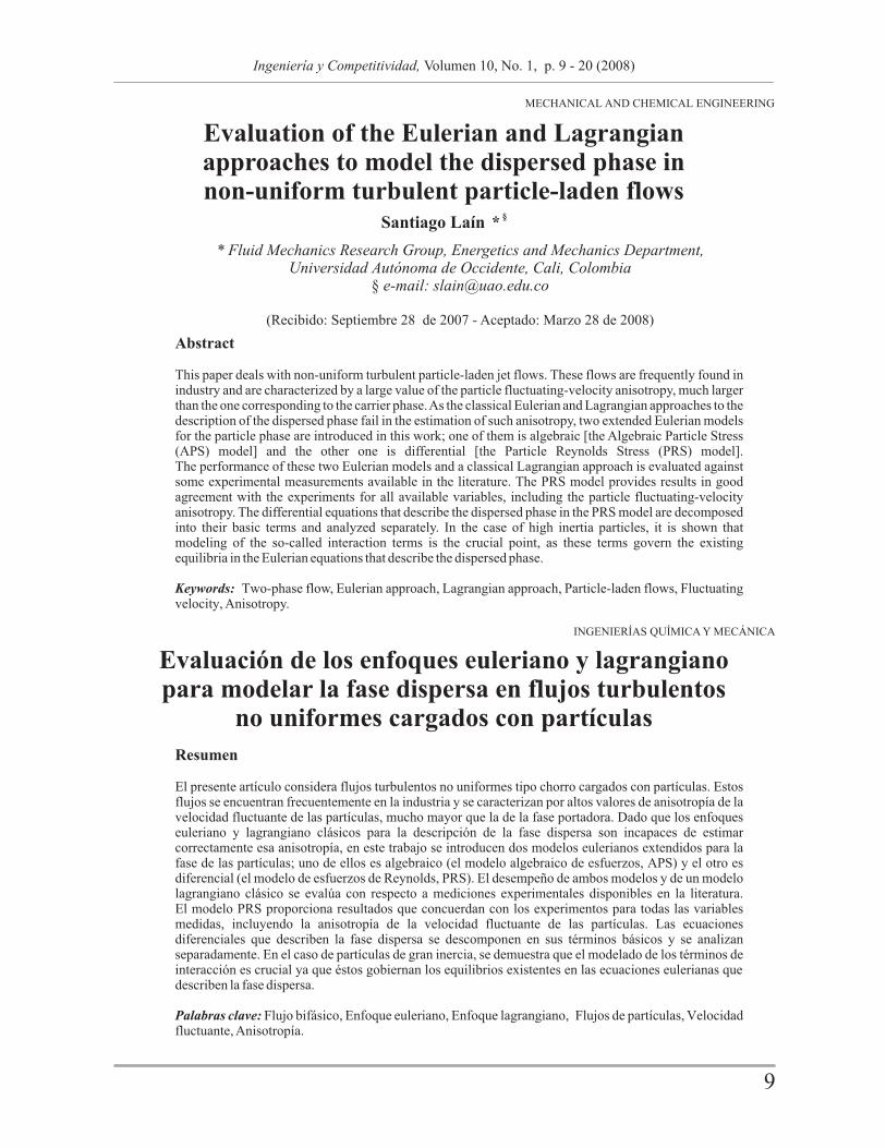
§ Santiago Laín * Abstract This paper deals with non-uniform turbulent particle-laden jet flows. These flows are frequently found in industry and are characterized by a large value of the particle fluctuating-velocity anisotropy, much larger than the one corresponding to the carrier phase. As the classical Eulerian and Lagrangian approaches to the description of the dispersed phase fail in the estimation of such anisotropy, two extended Eulerian models for the particle phase are introduced in this work; one of them is algebraic [the Algebraic Particle Stress (APS) model] and the other one is differential [the Particle Reynolds Stress (PRS) model]. The performance of these two Eulerian models and a classical Lagrangian approach is evaluated against some experimental measurements available in the literature. The PRS model provides results in good agreement with the experiments for all available variables, including the particle fluctuating-velocity anisotropy. The differential equations that describe the dispersed phase in the PRS model are decomposed into their basic terms and analyzed separately. In the case of high inertia particles, it is shown that modeling of the so-called interaction terms is the crucial point, as these terms govern the existing equilibria in the Eulerian equations that describe the dispersed phase. Keywords: Two-phase flow, Eulerian approach, Lagrangian approach, Particle-laden flows, Fluctuating velocity, Anisotropy. Resumen El presente artículo considera flujos turbulentos no uniformes tipo chorro cargados con partículas. Estos flujos se encuentran frecuentemente en la industria y se caracterizan por altos valores de anisotropía de la velocidad fluctuante de las partículas, mucho mayor que la de la fase portadora. Dado que los enfoques euleriano y lagrangiano clásicos para la descripción de la fase dispersa son incapaces de estimar correctamente esa anisotropía, en este trabajo se introducen dos modelos eulerianos extendidos para la fase de las partículas; uno de ellos es algebraico (el modelo algebraico de esfuerzos, APS) y el otro es diferencial (el modelo de esfuerzos de Reynolds, PRS). El desempeño de ambos modelos y de un modelo lagrangiano clásico se evalúa con respecto a mediciones experimentales disponibles en la literatura. El modelo PRS proporciona resultados que concuerdan con los experimentos para todas las variables medidas, incluyendo la anisotropía de la velocidad fluctuante de las partículas. Las ecuaciones diferenciales que describen la fase dispersa se descomponen en sus términos básicos y se analizan separadamente. En el caso de partículas de gran inercia, se demuestra que el modelado de los términos de interacción es crucial ya que éstos gobiernan los equilibrios existentes en las ecuaciones eulerianas que describen la fase dispersa. Palabras clave: Flujo bifásico, Enfoque euleriano, Enfoque lagrangiano, Flujos de partículas, Velocidad fluctuante, Anisotropía. Evaluation of the Eulerian and Lagrangian approaches to model the dispersed phase in non-uniform turbulent particle-laden flows MECHANICAL AND CHEMICAL ENGINEERING Ingeniería y Competitividad, Volumen 10, No. 1, p. 9 - 20 (2008) Evaluación de los enfoques euleriano y lagrangiano para modelar la fase dispersa en flujos turbulentos no uniformes cargados con partículas INGENIERÍAS QUÍMICA Y MECÁNICA * Fluid Mechanics Research Group, Energetics and Mechanics Department, Universidad Autónoma de Occidente, Cali, Colombia § e-mail: [email protected] (Recibido: Septiembre 28 de 2007 - Aceptado: Marzo 28 de 2008) 9
Transcript of INGENIERÍAS QUÍMICA Y MECÁNICA Evaluación de los...
§Santiago Laín *
Abstract
This paper deals with non-uniform turbulent particle-laden jet flows. These flows are frequently found in industry and are characterized by a large value of the particle fluctuating-velocity anisotropy, much larger than the one corresponding to the carrier phase. As the classical Eulerian and Lagrangian approaches to the description of the dispersed phase fail in the estimation of such anisotropy, two extended Eulerian models for the particle phase are introduced in this work; one of them is algebraic [the Algebraic Particle Stress (APS) model] and the other one is differential [the Particle Reynolds Stress (PRS) model]. The performance of these two Eulerian models and a classical Lagrangian approach is evaluated against some experimental measurements available in the literature. The PRS model provides results in good agreement with the experiments for all available variables, including the particle fluctuating-velocity anisotropy. The differential equations that describe the dispersed phase in the PRS model are decomposed into their basic terms and analyzed separately. In the case of high inertia particles, it is shown that modeling of the so-called interaction terms is the crucial point, as these terms govern the existing equilibria in the Eulerian equations that describe the dispersed phase.
Keywords: Two-phase flow, Eulerian approach, Lagrangian approach, Particle-laden flows, Fluctuating velocity, Anisotropy.
Resumen
El presente artículo considera flujos turbulentos no uniformes tipo chorro cargados con partículas. Estos flujos se encuentran frecuentemente en la industria y se caracterizan por altos valores de anisotropía de la velocidad fluctuante de las partículas, mucho mayor que la de la fase portadora. Dado que los enfoques euleriano y lagrangiano clásicos para la descripción de la fase dispersa son incapaces de estimar correctamente esa anisotropía, en este trabajo se introducen dos modelos eulerianos extendidos para la fase de las partículas; uno de ellos es algebraico (el modelo algebraico de esfuerzos, APS) y el otro es diferencial (el modelo de esfuerzos de Reynolds, PRS). El desempeño de ambos modelos y de un modelo lagrangiano clásico se evalúa con respecto a mediciones experimentales disponibles en la literatura. El modelo PRS proporciona resultados que concuerdan con los experimentos para todas las variables medidas, incluyendo la anisotropía de la velocidad fluctuante de las partículas. Las ecuaciones diferenciales que describen la fase dispersa se descomponen en sus términos básicos y se analizan separadamente. En el caso de partículas de gran inercia, se demuestra que el modelado de los términos de interacción es crucial ya que éstos gobiernan los equilibrios existentes en las ecuaciones eulerianas que describen la fase dispersa.
Palabras clave: Flujo bifásico, Enfoque euleriano, Enfoque lagrangiano, Flujos de partículas, Velocidad fluctuante, Anisotropía.
Evaluation of the Eulerian and Lagrangian approaches to model the dispersed phase in non-uniform turbulent particle-laden flows
MECHANICAL AND CHEMICAL ENGINEERING
Ingeniería y Competitividad, Volumen 10, No. 1, p. 9 - 20 (2008)
Evaluación de los enfoques euleriano y lagrangianopara modelar la fase dispersa en flujos turbulentos
no uniformes cargados con partículas
INGENIERÍAS QUÍMICA Y MECÁNICA
* Fluid Mechanics Research Group, Energetics and Mechanics Department, Universidad Autónoma de Occidente, Cali, Colombia
§ e-mail: [email protected]
(Recibido: Septiembre 28 de 2007 - Aceptado: Marzo 28 de 2008)
9
Regarding the dispersed phase in a two-phase flow (solid, droplet or bubble suspensions), it is mainly described by using one of two theoretical approaches. In the so-called Lagrangian method, the discrete elements are tracked through a turbulent-flow field by solving their equations of motion. In the so-called Eulerian method, the phases are handled as two interpenetrating continua and are governed by a set of differential equations representing conservation laws. Two possibilities come out for establishing the dispersed element equations. Firstly, the second phase can be considered as a fluid, for all effects. This corresponds to the well-known two-fluid model. Secondly, the non-continuous phase can be regarded as a cloud of material elements, whose behavior, depending on the variables of each element, is governed by a probability density function (PDF) that obeys a kinetic transport equation similar to the Maxwell-Boltzmann equation. The continuum equations for the second phase are obtained by taking the statistical moments of such PDF evolution equation.
In both cases, however, the underlying physics is the same, which can be described as follows. A large number of particulate trajectories (called trajectory realizations) are considered, and by averaging over these realizations, the required quantities, such as number density, mean particle velocities and particle velocity fluctuations, are derived. However, in the Eulerian approach, the trajectory constructions and the subsequent averaging are not explicitely carried out at a computational level. Instead, these operations are implicitely achieved at a conceptual level, so the discrete character of the underlying process is ‘washed out’ to provide a theory involving a continuum associated with the particles.
As the conceptual part of the work is carried out by the brain (not by a computer), Eulerian codes are fast-running, which makes them attractive from an engineering point of view.
The price paid for this computational efficiency is that by relying on intensive modeling, assumptions must be introduced to succeed in the closure of the particle fluctuating correlations. Conversely, in the Lagrangian approach, trajectory realizations are explicitely simulated by
the computer which also carries out the subsequently-required averaging. The price paid is more time-consuming runs.
However, the traditional closures, even giving approximate values for the mean fields, fail for the prediction of the particle velocity fluctuations, specially for non-uniform flows. To overcome this fact, considerable effort has been devoted to develop turbulence closures at the level of second moments of the particulate phase (Reeks, 1993; Wang et al., 1997; Hyland et al., 1998; Simonin, 1991). In fact, the traditional Lagrangian strategies for modeling the particle phase, grossly underpredict the anisotropy of the particle velocity fluctuation in non-uniform flows such as jets (Berlemont et al., 1997; Chen, 2000). On the other hand, the classical Eulerian methods make no attempt to predict such anisotropy. Moreover, after reviewing a number of experimental results, Laín & Aliod (2000) suggested that in axisymmetric jet flows laden with high inertia particles, the streamwise and transversal velocity fluctuations of the solid phase could hold the approximate
2 2 relationship (u) / (v) 10, as soon as a developed
2 flow is reached. Here, (u) corresponds to the axial
2 fluctuating velocity and (v) corresponds to the
radial one. Such a ratio is much larger than the one corresponding to the continuous phase, which is of order unity. Therefore, there is a need for improving the existing two-phase flow models to reproduce the particle fluctuating velocity anisotropy that is observed in non-uniform turbulent flow configurations.
The purpose of this paper is to propose and evaluate simple, computationally efficient, dispersed-phase Eulerian second-order models to improve the prediction of the particle fluctuating-velocity anisotropy in non-uniform jet flows. In that direction, two Eulerian stress models, one of them algebraic [the Algebraic Particle Stress (APS) model] and the other one differential [the Particle Reynolds Stress (PRS) model], are presented and evaluated together with a classical Lagrangian approach for the configuration of axisymmetric turbulent particle-laden free jet. The computational results are compared with the measurements of Mostafa et al. (1989). As a result, the differential version of the Eulerian stress model provides a good
1. Introduction
The subject of two or multiphase flow has become increasingly important in a wide variety of engineering systems for their optimum design and the safety of operations. However, that subject is not limited to modern industrial technology, and multiphase flow phenomena are present in a number of biological and natural systems that require a better understanding. As relevant applications of multiphase flow, we can cite, among others, power systems (boiling and pressurized water nuclear reactors), power plants with boilers and evaporators, geothermal energy plants, heat transfer systems (heat exchangers, evaporators, condensers, spray cooling towers, film cooling systems), process systems (fluidized beds, chemical reactors, stirred tank reactors, porous media), transport systems (air-lift pumps, pneumatic conveyors, ejectors), lubrication systems (two-phase flow lubrication, bearing cooling by cryogenics), environmental control (refrigerators, dust collectors, sewage treatment plants, air pollution control, life support systems for space applications), geo-meteorological phenomena (sedimentation, soil erosion, sand dune formations, river floodings, physics of the clouds) or biological systems (respiratory system, capillary transport, blood flow).
On the other hand, as the size of engineering systems becomes larger and the operating conditions are being pushed to new limits, the precise understanding of the physics governing these multiphase flow systems is paramount for safe and economically-sound operations. This means a shift of design methods from those exclusively based on static experimental correlations to the ones based on mathematical models that can predict dynamical behavior of systems such as transient responses and stabilities. The optimum design, the prediction of operational limits and, very often, the safe control of a great number of systems depend on the availability of realistic and accurate mathematical models of two-phase flow. However, such models are complex and not amenable to analytical solution; therefore, they must be solved numerically by properly implementing Computational Fluid Dynamics (CFD) simulation tools. The potential of CFD to address phenomena related with
multiphase flow in process industries was highlighted in the Winter 2002 issue of The Bridge, a quaterly journal of the National Academy of Engineering (Davidson, 2002).
In this paper, our interest is focused on dispersed two-phase gas-particle dilute flows, which pervade the chemical, pharmaceutical, agricultural and mining industries. In that context, the solid particles (discrete elements) are the dispersed phase and the gas is the continuous phase. Dilute flow is characterized by a volume
-3fraction occupied by the particles of less than 10 , which, in a cubic array, corresponds to an interparticle spacing of eight particle diameters. In such conditions, inter-particle collisions can be neglected (Crowe et al., 1998).
To describe the dynamics of the dispersed phase in a turbulent two-phase f low, some continuous-phase properties are required, such as the mean fluid velocity and the root-mean-square fluctuating fluid velocities (i.e., the flow turbulent characteristics). These properties are obtained either from experimental work or some appropriate computational procedure for predicting the turbulent flow field. For this purpose, methods such as Direct Numerical Simulation (DNS) or Kinematic Simulation (KS) provide unique opportunities to study specific effects like particle trapping in eddies (Eaton & Fessler, 1994) but are limited to small Reynolds number flows (DNS) or do not incorporate all of the physics involved in the Navier-Stokes equations (KS). Large eddy simulations (LES) allows one to handle complex flows (Wang et al., 1997) but the computational requirements are substantial, so these models are not used widely. The best quality / price ratio is, up to now, obtained by using the so-called Reynolds Averaged Navier-Stokes (RANS) equations, e.g., k-ε (or any or its variants) or Reynolds stress formulations. This kind of models consists of a set of partial differential equations expressing conservation laws for different time-averaged variables, e.g., continuity, momentum, turbulent kinetic energy, dissipation rate, etc. Moreover, these models have to be supplemented with several extra terms, the interaction terms, to account for the influence of the dispersed phase on the turbulence (the so-called two-way coupling).
10 11
Ingeniería y Competitividad, Volumen 10, No.1, p. 9 - 20 (2008) Ingeniería y Competitividad, Volumen 10, No. 1, p. 9 - 20 (2008)
d
iid
d
kk 2
1d
(6)
Fluctuating kinetic energy equation
dHere, V, , υ are the ensemble-averaged dispersed-elements velocity, volume fraction, and
fluctuating velocity with respect to V, υ υV.d is the density of the discrete elements and is
D d d p supposed to be constant. I (UV ) / j j j
is the standard interaction term due to the aerodynamic drag (U represents the fluid mean j
dV d dvelocity), the volumetric forces f ( )g j j
take into account the weight and the buoyancy. is the standard production term
Walso found in single phase flow and I is the fluctuating work exchangedwith the fluid.
WIt is worth to remember the closure for I :
where
is the particle relaxation time defined as the rate of response of particle acceleration to the relative velocity between the particle and the carrier fluid.
is the Lagrangian time-scale of the fluid flow L
turbulence defined in terms of the turbulent kinetic energy of the gas flow, k, and its dissipation rate, .
In this work, these variables are known from previous continuous-phase computations.
The performance of the closure given by Eqs. (7a-d) for axisymmetric jets laden with high inertia particles has been assessed by Laín & Aliod
d(2000), who made a very accurate prediction of k for a set of experiments corresponding to such a configuration.
However, the model given by Eqs. (4)-(6) can only dbe solved for k ; therefore, it is unable to provide
a n y i n f o r m a t i o n a b o u t t h e p a r t i c l e fluctuating-velocity anisotropy. To obtain some estimation of that anisotropy, the former model must be extended somehow.
The transport equations that govern the particle velocity correlations can be found in different works, for example, Simonin (1991). For dilute flows, by neglecting collisions between the discrete elements, the following expression can be written:
where represents the transport ofby particle velocity fluctuations, is the production contribution (which does not need to be defined as a positive quantity):
and is the exchanged work rate between the dispersed phase and the fluid, and is expressed as:
ji
d
jidd VP ,
4.0
k
kkI
L
PL
L
d
P
ddw
(7a)
Re3
4d
p
pD
p
C
d
d ji
,
Wij
dij
dij
d
jidd
IPDDt
D
(8)
ijD ,
d
ji d
ijP
,,d
ij mi
d
mjmj
d
mid VVP (9)
WijI
,,,
d Wddj
d
jddd
jd
jdd
tdd IPkkVk
(7b)
(7c)
(7d)
agreement for all availables quantities, such as the mean and fluctuating velocities for both phases, gas and particles. Moreover, the dispersed-phase equations for the momentum and fluctuating velocities of the PRS model are decomposed into their contributions (convection, diffusion, source, and interaction) which allows one to obtain a global picture of the momentum and fluctuating energy transfer in the jet.
2. Lagrangian approach
In the Lagrangian framework, a single particle of the dispersed phase is observed on its way through the flow field by solving the equations of the particle motion and the particle position. In this paper, we deal with solid particles with high inertia; therefore, by performing an order of magnitude analysis of the relevant time scales of the flow system, a reduced form of the particle equation of motion can be obtained that considers only the drag and gravity / buoyancy forces. In the end, the following system of equations has to be solved:
The drag coefficient C is given as follows:D
In the above equations [Eqs. (1)-(3)] the superscript d is used to identify a single particle, and x are the components of the instantaneous i i
particle velocity and position, respectively, d is p
the particle diameter, ρ is the density and g is the i
component of the acceleration of gravity. The particle Reynolds number is defined
, itix
14
3d,
di
p
iiiiDti g
d
uuC
(1)
(2)
1000Re 44, .0C
1000Re Re6
11
Re
24C
p
p66.0
D
p
p
D
(3)
as where is the dynamic
viscosity of the fluid.
The instantaneous fuid velocity along the i
particle trajectory was obtained by applying the Langevin equation model (for details, see Sommerfeld et al., 1993).
To obtain the relevant information about the underlying flow field, the continuous-phase equations have to be solved as well. Therefore, the time-averaged Navier-Stokes equations were solved in connection with an appropriate turbulence model. These equations include particle source terms (or interaction terms) to take the effect of two-way coupling into account. These source terms were calculated by using a modified version of the particle-source-in-cell (PSI-cell) approximation of Crowe et al. (1977). A detailed description of this procedure was given by Kohnen et al. (1994).
3. Dispersed-phase Eulerian transport equations
In the context of isothermal dilute flows (Laín & Aliod, 2000), by using the dispersed-elements-PDF-indicator function-ensemble conditioned average (Aliod & Dopazo, 1990; Zhang & Prosperetti, 1994), the following equations for the dispersed phase (consisting in a population of solid particles of equal diameter d ) are initially p
considered:
Mass conservation equation:
Momentum conservation equation:
0 ,,
d iidd
t
d V
dVj
Dj
,,
d
fI
VVV
,i
dij
dd
ijidd
tjd
(4)
(5)
, for
for
, /Re υu pp d
12 13
Ingeniería y Competitividad, Volumen 10, No.1, p. 9 - 20 (2008) Ingeniería y Competitividad, Volumen 10, No. 1, p. 9 - 20 (2008)

WiiI
with C = 0.4. Eq. (15) can be regarded as a L
‘natural’ extension of Eq. (7). By collecting Eqs. (13), (15) and substituting them into Eq. (10), can be expressed as:
Together with Eqs. (16) and (11), Eq. (13) is a system of three equations for the particle fluctuating velocity correlations (i = j) that can be solved once those expressions for the fluid stresses
d and k are provided.
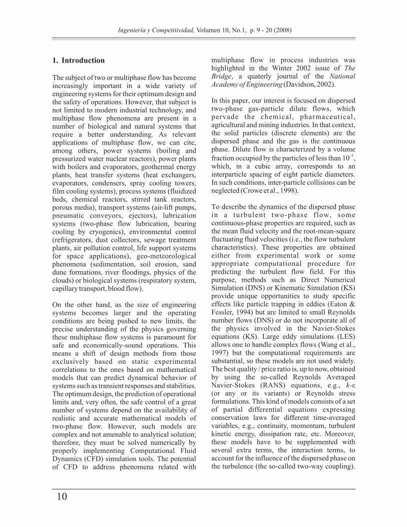
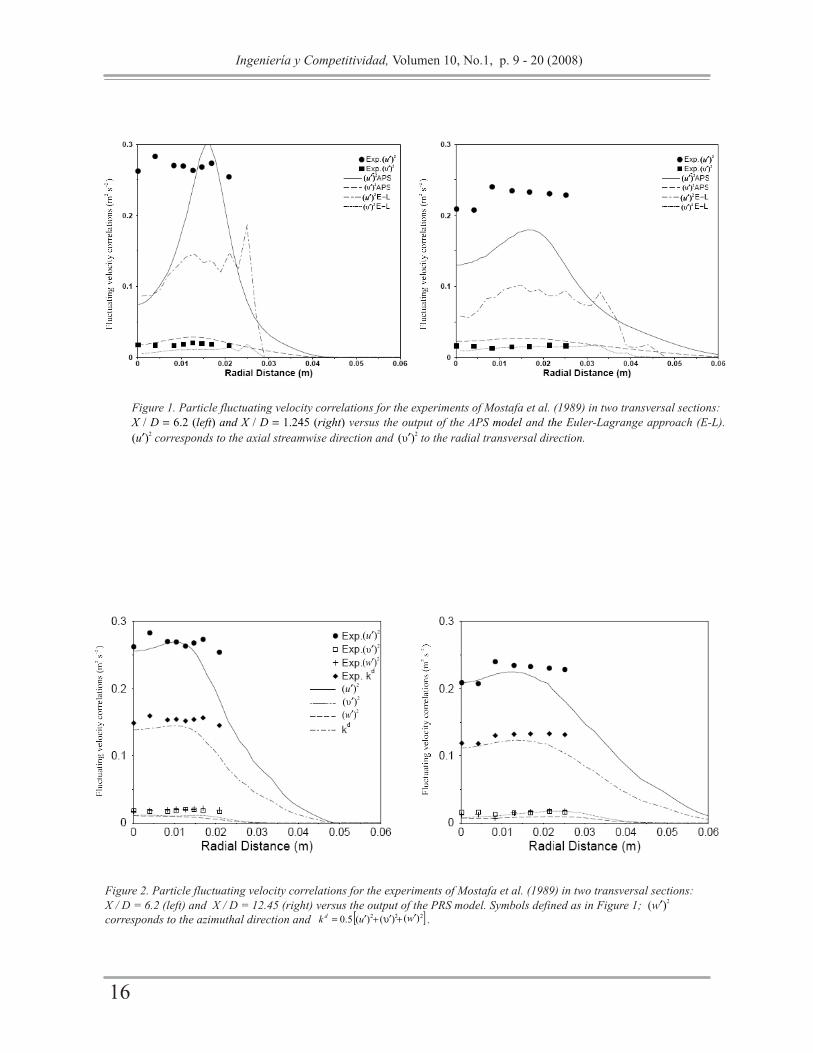
Figure 1 presents the results obtained from both the Euler-Lagrange approach (E-L) and the APS model as compared to the experimental measurements of Mostafa et al. (1989). In that figure, the particle fluctuating velocity correlations, in the axial direction ( ) and in the radial direction ( ), are shown as compared to the experiments of Mostafa et al. (1989) on a particle-laden round free jet and the output of the classical Euler-Lagrange approach (Sommerfeld et al., 1993) for two sections, X / D = 6.2, X / D = 12.45. X stands for the distance downstream of the nozzle and D for the diameter. It is noteworthy that the Euler-Lagrange approach provides acceptably accurate values for all fluid variables, including the Reynolds stresses and the mean velocities of the particles, but it considerably underpredicts their axial fluctuating component. This is a typical situation that also appears in the classical two-fluid model (Issa & Oliveira, 1998).
While the results for the transversal direction are similar in both calculation strategies (even the Euler-Lagrange method seems to work somewhat better), the situation is different for the streamwise component. In both cases, that component is underpredicted, particularly in the symmetry axis, but the APS-model version is noticeably closer to the experiments.
In spite of the fact that the performance of the APS model is not very accurate, the improvements made are encouraging to expect that a simplified Particle Reynolds Stress (PRS) model may enhance the quality of the predictions even more. This task will be carried out in the next section.
d
xxu '2 d
rr 2
5. Particle Reynolds Stress (PRS) model
The proposed model is based on the set of Eqs. (8), (9) and (16). Also, as previously stated, for non-uniform, strongly anisotropic flows laden with high-inertia particles, the closure for the particle shear stresses, given by Eq. (11), will be assumed.
The term that represents the transport by particle velocity fluctuations in Eq. (8) is closed, for practical purposes, by using a Boussinesq approximation (Wang et al., 1997):
where an implicit summation in subscript k is now indicated. stands for the turbulent Schmidt numbers and in our case we only need to consider the case i = j. The values chosen for these numbers are and(where w is the azimuthal direction). The election
d of was suggested by the value used in the k equation (Laín & Aliod, 2000), whereas for
and the simplest value of 1.0 was assigned because the performance of the PRS model does not depend appreciably on that value . In summary, the proposed PRS model consists of the system of three equations [Eqs. (8) with i = j ], the definition of given by Eq. (9) and the closures given by Eqs. (11), (16) and (17).
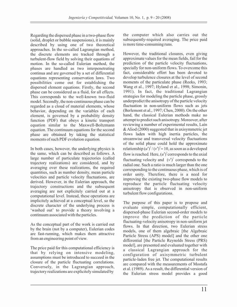
Comparisons with the experiments of Mostafa et al. (1989) are shown for the two transversal sections X / D = 6.2, X / D = 12.45. In Figure 2, the calculated profiles for the three particle fluctuating velocity correlations (and the kinetic energy calculated from them) are plotted versus the experimental data. It is remarkable that the anisotropy of particle fluctuating velocity correlations is well captured, in spite of the simplicity of the model, which only presents three extra equations with respect to the standard models.
iiWii
d
iiiip
dd
uuI (16)
,
,,
k
k
d
jidij
dd
ijD
(17)
dij
0.1 dww
drr 3.0d
xx
dxx
drr
dww
dijP
where u stands for the fluctuating velocity of the fluid with respect to the ensemble-averaged value .
By following the theoretical work of Reeks (1993) and Zaichik (1997), the Boussinesq-Prandtl hypothesis is feasible for modeling the particle shear stresses, in the limit of large inertial particles in simple shear flows, as considered in this work. These stresses are decomposed into a homogeneous component, whose structure is the same as if the local carrier flow were homogeneous, and a deviatoric component that involves terms proportional to the mean shear of the dispersed and the carrier flows. However, for long particle response times, the deviatoric component dominates over the homogeneous contribution reaching a finite value of
where is the long-time particle diffusion dcoefficient in the transverse direction and S is
the shear gradient of the dispersed phase. In addition, the particle diffusivity momentum
dcoefficient, , is said to be proportional to in
this limit. Therefore, in spite of the fact that the diffusivity momentum should be a tensor, in the
dlimit stated, can be written as a scalar quantity. In this context, the following expression for the particle shear stresses can be written:
with ; (x, r) denote the axial and transversal coordinates, respectively. The closure given by Eq.(11) will be assumed in the following to be valid in the cases considered in this work.
4. Algebraic Particle Stress (APS) model
As the simplest approximation, an algebraic model formulation for the particle normal stresses can be proposed by extending the ideas of the Algebraic Stress Model (ASM) developed by Rodi (1972) for single phase flow. The assumption is that the sum of convection and diffusion terms
of the transport equations for particle velocity correlations, is proportional to the sum of the convection and diffusion terms of the particle
dturbulent kinetic energy k :
where D d represents the transport by particle kdvelocity fluctuations of k . Substitution of Eqs. (6)
and (8) into Eq. (12), leads to the following approximate balance for the particle velocity correlations:
Here, the only non-closed terms appear in the fluid particle velocity correlation that is included in [Eq. (10)]. Simonin (1991) has worked out several methods for handling this fluid-particle velocity correlations, deriving algebraic as well as differential equations for them. Unfortunately, the required CPU time grows rapidly as the number of equations increases.
The approach proposed in this work is simpler. A relationship between the fluid-particle velocity correlation and the fluid and particle fluctuating velocity correlations is assumed as follows:
where the tensor is written as:
dS , 2
1
,, zrrxd
rxd VV (11)
p
d
rxdd
d
ii ,
Wii
dii
d
Wdd
dd
ii IPIP
k
(13)
WiiI
d
iiu
2
1iiii
d
ii
d
ii uuu (14)
ij
ijL
ij
ji
L
Lp
L
uuC
ij
ij
(15a)
(10)
dij
d
ji
d
ji
p
ddWij uuI
2
uU
Wdd
d
d
ii IPk
, k
ddd
d
d
iiii
d
iidd
DDt
kD
kD
Dt
Dd
(12)
[[
(15b)
14 15
Ingeniería y Competitividad, Volumen 10, No.1, p. 9 - 20 (2008) Ingeniería y Competitividad, Volumen 10, No. 1, p. 9 - 20 (2008)

WiiI
with C = 0.4. Eq. (15) can be regarded as a L
‘natural’ extension of Eq. (7). By collecting Eqs. (13), (15) and substituting them into Eq. (10), can be expressed as:
Together with Eqs. (16) and (11), Eq. (13) is a system of three equations for the particle fluctuating velocity correlations (i = j) that can be solved once those expressions for the fluid stresses
d and k are provided.
Figure 1 presents the results obtained from both the Euler-Lagrange approach (E-L) and the APS model as compared to the experimental measurements of Mostafa et al. (1989). In that figure, the particle fluctuating velocity correlations, in the axial direction ( ) and in the radial direction ( ), are shown as compared to the experiments of Mostafa et al. (1989) on a particle-laden round free jet and the output of the classical Euler-Lagrange approach (Sommerfeld et al., 1993) for two sections, X / D = 6.2, X / D = 12.45. X stands for the distance downstream of the nozzle and D for the diameter. It is noteworthy that the Euler-Lagrange approach provides acceptably accurate values for all fluid variables, including the Reynolds stresses and the mean velocities of the particles, but it considerably underpredicts their axial fluctuating component. This is a typical situation that also appears in the classical two-fluid model (Issa & Oliveira, 1998).
While the results for the transversal direction are similar in both calculation strategies (even the Euler-Lagrange method seems to work somewhat better), the situation is different for the streamwise component. In both cases, that component is underpredicted, particularly in the symmetry axis, but the APS-model version is noticeably closer to the experiments.
In spite of the fact that the performance of the APS model is not very accurate, the improvements made are encouraging to expect that a simplified Particle Reynolds Stress (PRS) model may enhance the quality of the predictions even more. This task will be carried out in the next section.
d
xxu '2 d
rr 2
5. Particle Reynolds Stress (PRS) model
The proposed model is based on the set of Eqs. (8), (9) and (16). Also, as previously stated, for non-uniform, strongly anisotropic flows laden with high-inertia particles, the closure for the particle shear stresses, given by Eq. (11), will be assumed.
The term that represents the transport by particle velocity fluctuations in Eq. (8) is closed, for practical purposes, by using a Boussinesq approximation (Wang et al., 1997):
where an implicit summation in subscript k is now indicated. stands for the turbulent Schmidt numbers and in our case we only need to consider the case i = j. The values chosen for these numbers are and(where w is the azimuthal direction). The election
d of was suggested by the value used in the k equation (Laín & Aliod, 2000), whereas for
and the simplest value of 1.0 was assigned because the performance of the PRS model does not depend appreciably on that value . In summary, the proposed PRS model consists of the system of three equations [Eqs. (8) with i = j ], the definition of given by Eq. (9) and the closures given by Eqs. (11), (16) and (17).
Comparisons with the experiments of Mostafa et al. (1989) are shown for the two transversal sections X / D = 6.2, X / D = 12.45. In Figure 2, the calculated profiles for the three particle fluctuating velocity correlations (and the kinetic energy calculated from them) are plotted versus the experimental data. It is remarkable that the anisotropy of particle fluctuating velocity correlations is well captured, in spite of the simplicity of the model, which only presents three extra equations with respect to the standard models.
iiWii
d
iiiip
dd
uuI (16)
,
,,
k
k
d
jidij
dd
ijD
(17)
dij
0.1 dww
drr 3.0d
xx
dxx
drr
dww
dijP
where u stands for the fluctuating velocity of the fluid with respect to the ensemble-averaged value .
By following the theoretical work of Reeks (1993) and Zaichik (1997), the Boussinesq-Prandtl hypothesis is feasible for modeling the particle shear stresses, in the limit of large inertial particles in simple shear flows, as considered in this work. These stresses are decomposed into a homogeneous component, whose structure is the same as if the local carrier flow were homogeneous, and a deviatoric component that involves terms proportional to the mean shear of the dispersed and the carrier flows. However, for long particle response times, the deviatoric component dominates over the homogeneous contribution reaching a finite value of
where is the long-time particle diffusion dcoefficient in the transverse direction and S is
the shear gradient of the dispersed phase. In addition, the particle diffusivity momentum
dcoefficient, , is said to be proportional to in
this limit. Therefore, in spite of the fact that the diffusivity momentum should be a tensor, in the
dlimit stated, can be written as a scalar quantity. In this context, the following expression for the particle shear stresses can be written:
with ; (x, r) denote the axial and transversal coordinates, respectively. The closure given by Eq.(11) will be assumed in the following to be valid in the cases considered in this work.
4. Algebraic Particle Stress (APS) model
As the simplest approximation, an algebraic model formulation for the particle normal stresses can be proposed by extending the ideas of the Algebraic Stress Model (ASM) developed by Rodi (1972) for single phase flow. The assumption is that the sum of convection and diffusion terms
of the transport equations for particle velocity correlations, is proportional to the sum of the convection and diffusion terms of the particle
dturbulent kinetic energy k :
where D d represents the transport by particle kdvelocity fluctuations of k . Substitution of Eqs. (6)
and (8) into Eq. (12), leads to the following approximate balance for the particle velocity correlations:
Here, the only non-closed terms appear in the fluid particle velocity correlation that is included in [Eq. (10)]. Simonin (1991) has worked out several methods for handling this fluid-particle velocity correlations, deriving algebraic as well as differential equations for them. Unfortunately, the required CPU time grows rapidly as the number of equations increases.
The approach proposed in this work is simpler. A relationship between the fluid-particle velocity correlation and the fluid and particle fluctuating velocity correlations is assumed as follows:
where the tensor is written as:
dS , 2
1
,, zrrxd
rxd VV (11)
p
d
rxdd
d
ii ,
Wii
dii
d
Wdd
dd
ii IPIP
k
(13)
WiiI
d
iiu
2
1iiii
d
ii
d
ii uuu (14)
ij
ijL
ij
ji
L
Lp
L
uuC
ij
ij
(15a)
(10)
dij
d
ji
d
ji
p
ddWij uuI
2
uU
Wdd
d
d
ii IPk
, k
ddd
d
d
iiii
d
iidd
DDt
kD
kD
Dt
Dd
(12)
[[
(15b)
14 15
Ingeniería y Competitividad, Volumen 10, No.1, p. 9 - 20 (2008) Ingeniería y Competitividad, Volumen 10, No. 1, p. 9 - 20 (2008)
6. Analysis of the momentum and fluctuating energy transfer in the jet
To get some insight into the mechanisms that drive the dynamics of the particle-laden turbulent round jet, the dispersed-phase equations for the momentum [Eq. (5)] and particle fluctuating velocity correlations [Eq. (8)] in a representative axial section are decomposed into four global contributions:
convection = diffusion + source + interaction
Here, the sources have been divided into two categories. On the one hand, the so-called interaction contribution is considered in the terms denoted by in the system of Eqs. (5) and (8) and, on the other hand, the rest of source terms, are grouped in the source contribution. The snapshots of these contributions, in a typical axial section, were lumped together and are shown in Figures 3 and 4. As follows from those figures, the formulation of the interaction terms plays a fundamental role in the Eulerian-like dispersed-phase equations because those terms govern the existing equilibria in the equations.
The following notation is adopted:
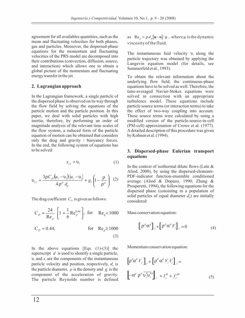
In the axial velocity equation shown on the left section of Fig. 3, the term (that represents the force exchanged between the phases) compensates the convective term, which determines the acceleration of the particle phase (the diffusion and source terms are negligible relative to the convective term). This fact expresses nothing else than Newton’s second law of motion, i.e., that the variation of the particle momentum is due to the forces that act on the particles. In this case, as the associated interaction term is negative, the particle phase delivers a linear momentum to the gas in the axial direction, decreasing the velocity of the particles.
d
rrdrr
d
xxd
xx
R
(u )R
2
xI
r
drr
dd R,
In the radial velocity equation (on the right section of Figure 3), beyond the zone near the symmetry axis, the most relevant contributions are the source and interaction terms, which are modulated by the convection term, the diffusion term being small enough relative to the other terms. The fact that the source terms equilibrate the interaction term implies that the expansion of the jet is performed at the expense of transferring linear momentum to the fluid. Moreover, the source term, , represents the force per unit volume responsible for the spreading of the jet (Lain & Aliod, 1999). This term comes from the potential energy per unit volume , where is the solid density and is the strength. Therefore, controls the spreading rate of the particles in the radial direction of the jet. This agrees with Reeks' conclusions in the limit of large particle inertia (Reeks, 1993). In consequence, the correct p r e d i c t i o n o f t h e e v o l u t i o n o f t h e profile depends on the accurate estimation of the particle radial fluctuating-velocity correlation.
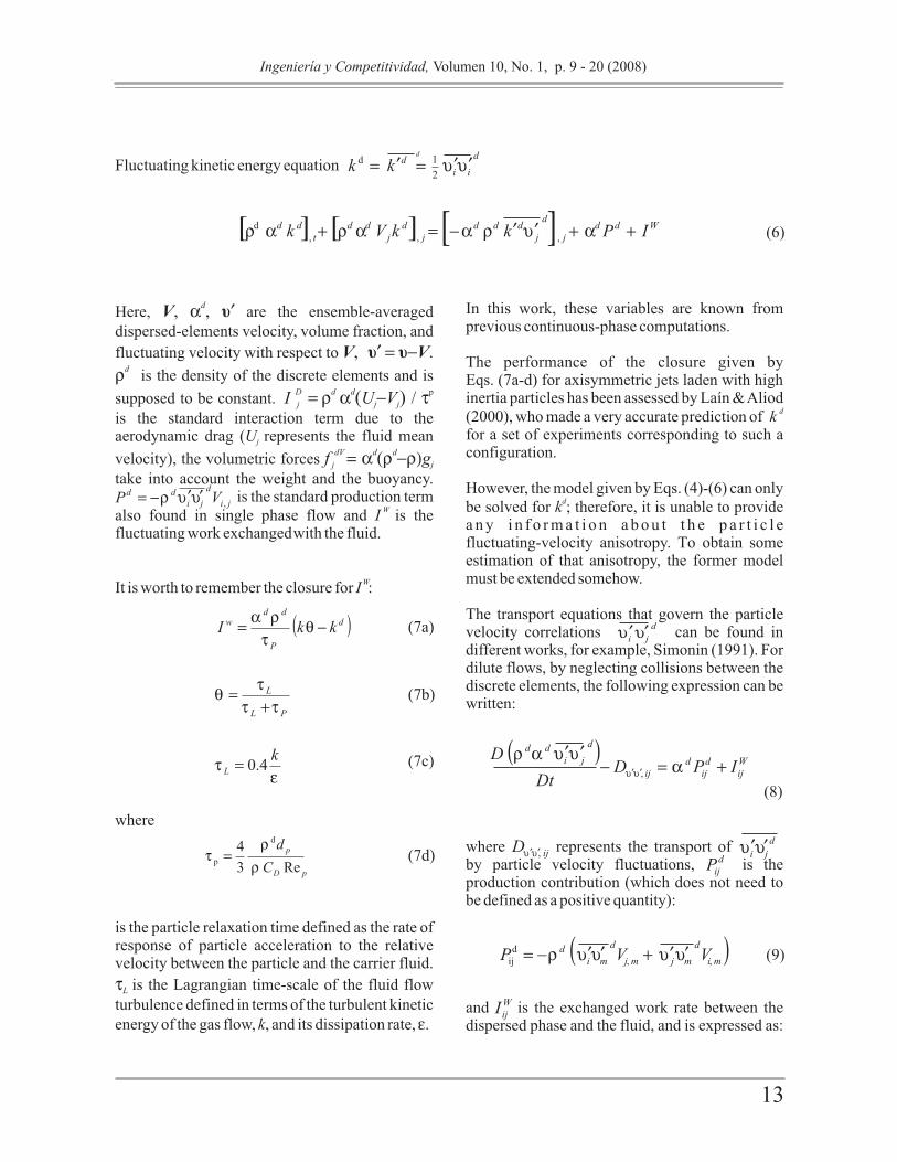
Figure 4 shows the behavior of the different contributions (convection, diffusion, source and interaction) in the particle fluctuating correlation, Eq. (8). Here, as happened with the particle momentum equations, the interaction termsare relevant contributions and should be taken into account. From the axial fluctuating-velocity correlation, , it follows (Fig. 4, top left) that the particulate phase transfers energy to the fluid, because the associated interaction term is negative. The convection term is roughly compensated with , while the diffusion and source (production) terms modulate this balance. Therefore, the change in is mainly due to the interchange of fluctuating work between the phases. is an intrinsic source of particle turbulence in the jet due to the interaction between the shear stresses and the radial component of the gradient of axial velocity . Part of this supplementary fluctuating energy is directly dissipated by the fluid and part of it is redistributed, via the continuous phase, to provide energy to the radial and azimuthal particle velocity fluctuations, as shown in Figure 4 (top right and bottom). In the plot for the particle radial fluctuating velocity correlation, , the production contribution is negative, i.e., it acts as a sink, mainly due to the interaction between
dxxR
WxxI
dxxR
dxxP
rxrx
d V ,
drrR
d
wwdwwR 2
(18a)
(18b)
(18c)
( ) 2
( )w
DxI
d d
rrR drrR
d
WxxI
drr
dd R
Figure 1. Particle fluctuating velocity correlations for the experiments of Mostafa et al. (1989) in two transversal sections: versus the output of the APS and Euler-Lagrange approach (E-L).
corresponds to the axial streamwise direction and υ to the radial transversal direction.
X / D 6.2 (left) and X / D 1.245 (right) model the 2 2(u) ( )
Figure 2. Particle fluctuating velocity correlations for the experiments of Mostafa et al. (1989) in two transversal sections: X / D = 6.2 (left) and X / D = 12.45 (right) versus the output of the PRS model. Symbols defined as in Figure 1; w corresponds to the azimuthal direction and .
2( )
2(u)2(u)2( )υ 2( )υ
2(u)2(u)2
( )υ2
( )υ2(u)2(u)2
( )υ2
( )υ
2(u)2(u)2( )υ 2( )υ
2(u)2(u)2
( )υ2
( )υ2(u)2(u)2
( )υ2
( )υ
2(u)2( )υ2(w)
2(u)2( )υ2(w)
[ ]225.0 (u )k d ()2 (w)
16 17
Ingeniería y Competitividad, Volumen 10, No.1, p. 9 - 20 (2008) Ingeniería y Competitividad, Volumen 10, No. 1, p. 9 - 20 (2008)

6. Analysis of the momentum and fluctuating energy transfer in the jet
To get some insight into the mechanisms that drive the dynamics of the particle-laden turbulent round jet, the dispersed-phase equations for the momentum [Eq. (5)] and particle fluctuating velocity correlations [Eq. (8)] in a representative axial section are decomposed into four global contributions:
convection = diffusion + source + interaction
Here, the sources have been divided into two categories. On the one hand, the so-called interaction contribution is considered in the terms denoted by in the system of Eqs. (5) and (8) and, on the other hand, the rest of source terms, are grouped in the source contribution. The snapshots of these contributions, in a typical axial section, were lumped together and are shown in Figures 3 and 4. As follows from those figures, the formulation of the interaction terms plays a fundamental role in the Eulerian-like dispersed-phase equations because those terms govern the existing equilibria in the equations.
The following notation is adopted:
In the axial velocity equation shown on the left section of Fig. 3, the term (that represents the force exchanged between the phases) compensates the convective term, which determines the acceleration of the particle phase (the diffusion and source terms are negligible relative to the convective term). This fact expresses nothing else than Newton’s second law of motion, i.e., that the variation of the particle momentum is due to the forces that act on the particles. In this case, as the associated interaction term is negative, the particle phase delivers a linear momentum to the gas in the axial direction, decreasing the velocity of the particles.
d
rrdrr
d
xxd
xx
R
(u )R
2
xI
r
drr
dd R,
In the radial velocity equation (on the right section of Figure 3), beyond the zone near the symmetry axis, the most relevant contributions are the source and interaction terms, which are modulated by the convection term, the diffusion term being small enough relative to the other terms. The fact that the source terms equilibrate the interaction term implies that the expansion of the jet is performed at the expense of transferring linear momentum to the fluid. Moreover, the source term, , represents the force per unit volume responsible for the spreading of the jet (Lain & Aliod, 1999). This term comes from the potential energy per unit volume , where is the solid density and is the strength. Therefore, controls the spreading rate of the particles in the radial direction of the jet. This agrees with Reeks' conclusions in the limit of large particle inertia (Reeks, 1993). In consequence, the correct p r e d i c t i o n o f t h e e v o l u t i o n o f t h e profile depends on the accurate estimation of the particle radial fluctuating-velocity correlation.
Figure 4 shows the behavior of the different contributions (convection, diffusion, source and interaction) in the particle fluctuating correlation, Eq. (8). Here, as happened with the particle momentum equations, the interaction termsare relevant contributions and should be taken into account. From the axial fluctuating-velocity correlation, , it follows (Fig. 4, top left) that the particulate phase transfers energy to the fluid, because the associated interaction term is negative. The convection term is roughly compensated with , while the diffusion and source (production) terms modulate this balance. Therefore, the change in is mainly due to the interchange of fluctuating work between the phases. is an intrinsic source of particle turbulence in the jet due to the interaction between the shear stresses and the radial component of the gradient of axial velocity . Part of this supplementary fluctuating energy is directly dissipated by the fluid and part of it is redistributed, via the continuous phase, to provide energy to the radial and azimuthal particle velocity fluctuations, as shown in Figure 4 (top right and bottom). In the plot for the part icle radial fluctuating velocity correlation, , the production contribution is negative, i.e., it acts as a sink, mainly due to the interaction between
dxxR
WxxI
dxxR
dxxP
rxrx
d V ,
drrR
d
wwdwwR 2
(18a)
(18b)
(18c)
( ) 2
( )w
DxI
d d
rrR drrR
d
WxxI
drr
dd R
Figure 1. Particle fluctuating velocity correlations for the experiments of Mostafa et al. (1989) in two transversal sections: versus the output of the APS and Euler-Lagrange approach (E-L).
corresponds to the axial streamwise direction and υ to the radial transversal direction.
X / D 6.2 (left) and X / D 1.245 (right) model the 2 2(u) ( )
Figure 2. Particle fluctuating velocity correlations for the experiments of Mostafa et al. (1989) in two transversal sections: X / D = 6.2 (left) and X / D = 12.45 (right) versus the output of the PRS model. Symbols defined as in Figure 1; w corresponds to the azimuthal direction and .
2( )
2(u)2(u)2( )υ 2( )υ
2(u)2(u)2
( )υ2
( )υ2(u)2(u)2
( )υ2
( )υ
2(u)2(u)2( )υ 2( )υ
2(u)2(u)2
( )υ2
( )υ2(u)2(u)2
( )υ2
( )υ
2(u)2( )υ2(w)
2(u)2( )υ2(w)
[ ]225.0 (u )k d ()2 (w)
16 17
Ingeniería y Competitividad, Volumen 10, No.1, p. 9 - 20 (2008) Ingeniería y Competitividad, Volumen 10, No. 1, p. 9 - 20 (2008)

the potential energy and the radial component of the gradient of radial velocity, . This contribution is interpreted as the power per unit volume that is required to spread the solids across the jet. Moreover, the interaction contribution is approximately compensated by the production term , which means that the work performed by the particle radial stress against the gradient of radial velocity (to spread the particles in the jet) is supplied by the exchange of energy between the phases. The balance between the different terms for the is rather similar to what happens with the equation (Figure 4, bottom). It is remarkable that the shape of the interaction term is very similar to that obtained by Wang et al. (1997) in a channel flow using a more complete formulation and large eddy simulations.
7. Conclusions
In this paper, an evaluation has been made on the performance of the Eulerian and Lagrangian modeling strategies for the dispersed phase in non-uniform dispersed two-phase flow. In the Eulerian frame, two second-order models have been proposed: an algebraic model, in the spirit of single phase flow, and a Reynolds stress differential model, in which only the equations for the three particle fluctuating velocity correlations had to be solved, while the calculation of the shear stresses relied on a Boussinesq approximation which has been justified theoretically and numerically. In the Lagrangian frame a classical approach is used (Sommerfeld et al., 1993).
The models have been applied to the configuration of particle-laden turbulent round jet and compared with the experiments of Mostafa et al. (1989). In fact, the Lagrangian approach is not adequate enough to describe the particle fluctuating velocity anisotropy. This also happens with the Eulerian algebraic stress model, although the results for the anisotropy are closer to the measurements. In the end, the differential particle Reynolds stress model provided a good agreement between calculations and experiments for all available variables of both phases, including the particle fluctuating velocity anisotropy.
The results obtained with the differential particle Reynolds stress model have been used to get a snapshot of the different contributions (convection, diffusion, source and interaction) that enter the differential equations for the dispersed phase. From an analysis of these terms, in a representative axial section, it has been possible to get a picture of the momentum and fluctuating energy transfer in the jet. It has been shown that the particle axial fluctuating velocity correlation component transfers fluctuating energy to the fluid; part of it increases the production and dissipation of turbulent energy in the continuous phase, and the rest is injected, via the fluid, in the transversal particle fluctuating velocity correlations and . Moreover, the accurate description of the spreading of particles across the jet requires the correct calculation of the particle radial fluctuating velocity .
8. Bibliographic references
Aliod, R. & Dopazo, C. (1990). A statistically conditioned averaging formalism for deriving two-phase flow equations. Particle and Particle Systems Characterization 7 (1-4), 191-202.
Berlemont, A., Desjonqueres, P. & Cabot, M.S. (1997). Turbulence modification in a particle laden wall jet. In Proceedings of ASME FEDSM 97, San Francisco, USA, Paper No. 3577.
Chen, X.-Q. (2000). Heavy particle dispersion in inhomogeneous, anisotropic, turbulent flows. International Journal of Multiphase Flow 26 (4), 635-661.
Crowe, C.T., Sharma, M.P. & Stock, D.E. (1977). The particle-source-in-cell (PSI-cell) method for gas-drople t f lows. Journal o f Flu ids Engineering,Transactions of the American Society of Mechanical Engineers 99 (2), 325-332.
Crowe, C.T., Sommerfeld, M. & Tsuji, Y. (1998). Multiphase flow with droplets and particles. Boca Raton, Florida: CRC Press.
Davidson, D.L. (2002). The role of computational fluid dynamics in process industries. The Bridge 32 (4), 9-14.
dxxR
drrR d
wwR
WrrI
drrP
drr
d R
dwwR d
rrR
3),2,1 (id
ii
dwwR
drr
dd R
rrV ,
Figure 3. Snapshot of the balance of the different terms in the particle momentum equations (in a typical section) for the experiment of Mostafa et al. (1989): axial momentum (left) and radial momentum (right).
Figure 4. Snapshots of the terms in the equations for the fluctuating velocity correlations of the dispersed phase in the axial station X / D = 12.45 for the experiments of Mostafa et al. (1989).
1918
Ingeniería y Competitividad, Volumen 10, No.1, p. 9 - 20 (2008) Ingeniería y Competitividad, Volumen 10, No. 1, p. 9 - 20 (2008)
Eaton, J.K., & Fessler, J.R. (1994). Preferential concentration of particles by turbulence. International Journal of Multiphase Flow 20 (Suppl. 1), 169-209.
Février, P. & Simonin, O. (1998). Constitutive relations for fluid-particle velocity correlations in gas-solid turbulent flows. In Proceedings of the Third International Conference on Multiphase Flow (ICMF´98), Lyon, France, Paper No. 538.
Hyland, K.E., Simonin, O., & Reeks, M.W. (1998) On the continuum equations for two phase flows. In Proceedings of the Third International Conference on Multiphase Flow (ICMF´98), Lyon, France, Paper No. 567.
Issa, R.I. & Oliveira, P.J. (1998). Accounting for non-equilibrium turbulent fluctuations in the Eulerian two-fluid model by means of the notion of induction period. In Proceedings of the Third International Conference on Multiphase Flow, (ICMF´98) Lyon, France, Paper No. 307.
Kohnen, G., Rüger, M. & Sommerfeld, M. (1994). Convergence behaviour for numerical calculations by the Euler / Lagrange method for strongly coupled phases. In: C.T. Crowe, R. Johnson, A. Prosperetti, M. Sommerfeld, & Y. Tsuji (editors), Numerical Methods for Multiphase Flow FED 185, p. 191-202. American Society of Mechanical Engineers (ASME, FED).
Laín, S. & Aliod, R. (1999). Analysis and discussion on the Eulerian dispersed particle equations in non-uniform turbulent gas-solid two-phase flows. In: W. Rodi & D. Laurence (editors), Proceedings of the Fourth International Symposium on Engineering Turbulence Modelling and Measurements, Ajaccio, Corsica, France, p. 923-932. Elsevier Science & Technology Books.
Laín, S. & Aliod, R. (2000). Deduction and validation of an Eulerian-Eulerian model for turbulent dilute two-phase flows by means of the phase indicator function-disperse elements probability density function. Chinese Journal of Chemical Engineering 8 (3), 189-202.
Mostafa, A.A., Mongia, H.C., McDonell, V.G., & Samuelsen, G.S. (1989). Evolution of particle-laden jet flows: a theoretical and experimental study. American Institute of Aeronautics and Astronautics Journal 27 (2), 167-183.
Reeks, M.W. (1993). On the constitutive relations for dispersed particles in non-uniform flows.I: Dispersion in a simple shear flow. Physics of Fluids A 5 (3), 750-761.
Rodi, W. (1972) The prediction of free turbulent boundary layers by use of a two-equation model of turbulence. Doctoral Thesis, Imperial College, University of London, London, United Kingdom.
Sommerfeld, M., Kohnen, G. & Rüger, M. (1993). Some open questions and inconsistencies of Lagrangian particle dispersion models. In Proceedings of the 9th Symposium on Turbulent Shear Flows, Kyoto, Japan, Paper No. 15-1.
Simonin, O. (1991). Prediction of the dispersed phase turbulence in particulate laden jet. In Proceedings of the Fourth International Symposium on Gas-Solid Flows, American Society of Mechanical Engineers (ASME, FED), Vol. 121, p. 197-206.
Wang, Q., Squires, K.D. & Simonin, O. (1997). Large eddy simulation of turbulent gas-solid flows in a vertical channel and evaluation of second-order models. International Journal of Heat and Fluid Flow 19 (5), 505-511.
Zaichik, L.I. (1997). Modelling of the motion of particles in non-uniform turbulent flow using the equation for the probability density function. Journal of Applied Mathematics and Mechanics 61 (1), 127-133.
Zhang, D.Z., & Prosperetti, A. (1994). Averaged equations for inviscid disperse two-phase flow. Journal of Fluid Mechanics 267, 185-219.
20
Ingeniería y Competitividad, Volumen 10, No.1, p. 9 - 20 (2008)