Infrared spectroscopy of acetylene

by Dr. G. Bradley Armen

Department of Physics and Astronomy 401 Nielsen Physics Building The University of Tennessee

Knoxville, Tennessee 37996-1200

Copyright © April 2007 by George Bradley Armen* *All rights are reserved. No part of this publication may be reproduced or transmitted in any form or by any means, electronic or mechanical, including photocopy, recording, or any information storage or retrieval system, without permission in writing from the author. A: INTRODUCTION

Molecules form an interesting bridge between larger, classical objects and smaller

systems such as atoms. Because of their size and structure, we can observe motions we have a classically intuitive notion of in the quantum regime. In particular we’ll get some insight into rotational and vibrational motions at the quantum level. In this laboratory we will study the infrared (IR) absorption of acetylene molecules, relating the observed spectrum to the molecule’s structure. Furthermore, we’ll see very directly the consequences of Boltzmann’s thermal distribution, which is fundamental to many areas of physics.

To explore all this, we’ll make use of an interesting and important laboratory tool: the Fourier transform infrared (FTIR) spectrometer. As physicists, the spectrometer is of interest to us simply because of its nature: It’s a direct application of the famous Michelson interferometer (of introductory physics courses) to very practical problems. While the FTIR is a standard laboratory item, one should appreciate all of the very difficult technical problems that needed solution before it could become an off-the-shelf piece of equipment.

In this laboratory you should come away with 1.) Some of the basic ideas of molecular spectroscopy in the IR regime.

2.) Experience in using, and an understanding of, the FTIR spectrometer. 3.) Some detailed understanding of H2C2 motion at the quantum level, and therefore… 4.) an increased knowledge of molecular physics, and maybe some increased insight into quantum mechanics in general.

B: THEORY

This section outlines some of the basics of molecular physics. Molecular

structure and dynamics is an important branch of physics, although in recent years the subject has been preempted by the physical chemists. It’s important to us because it highlights some very basic and fundamental quantum mechanics. In particular, describing vibrational motion provides a good introduction to the basic concepts behind field theory. Additionally, rotational spectra demonstrate in a very direct way the statistical nature of quantum systems in equilibrium at room temperature. The following discussion is intended to give us a basic appreciation of what we’re seeing in (and practical help in analyzing) the acetylene FTIR spectra.

1. Overview The theory of molecular structure begins by a separation of motions occurring on

very different time scales. To solve for the quantum structure of a molecule, one begins by specifying the coordinates1 for each nucleus ( ni Ni ,..1 =R ) and each electron ( ei Ni ,..1 =r ). The Hamiltonian can be written as

elelelnucelnucnucnuc VVKVKH −−− ++++= . The nuclear Hamiltonian nucnucnuc VK −+ contains the kinetic and nuclear-nuclear Coulomb repulsion energies. The remaining terms describe electronic motion: Kinetic ( elK ),

1 We should also include spin coordinates to be complete. We’ll do so later when it’s needed.

electron-nuclei Coulomb attraction ( elnucV − ), and electron-electron Coulomb repulsion ( elelV − ).

It quickly becomes obvious that, since the nuclei are so much more massive than the electrons, a reasonable approximation (Born-Oppenheimer) is to first consider the nuclei fixed in some configuration iR . We can then solve for the motion of the speedy electrons. The resulting electronic wave function elψ depends on the nuclear coordinates parametrically. The total wave function is thus approximated by the separation

):,(t),( ijelinucT t RrR ψψψ ×= ,

where nucψ is the wave function describing the actual nuclear motion. With this separation we can find stationary electronic eigenstates whose energies also depend parametrically on the iR :

)(

):()():( ,,

ielnucelelelel

ijnelinijnelel

VVKH

EH

R

RrRRr

−− ++≡

= ψψ

.

Now, using the Born-Oppenheimer scheme we assume that as the nuclei move, i.e.

iii RRR δ+→ , the electrons in their eigenstate ):(, ijnel Rrψ instantly accommodate to the new nuclear configuration, remaining in the same eigenstate level n:

):():( ,, iijnelijnel RRrRr δψψ +→ .

This is the adiabatic approximation, referring to the evolution of a wave function undergoing slow changes in its potential. The electronic energy )( inE R appears as an added potential in the nuclear equation of motion

nucnucnnucnucnuc tiEVK ψψ

∂∂

=++ − )( .

Now we can solve for the dynamics of the nuclear motion – given that the electronic motion is constrained to a certain stationary state n. The electronic state of the molecule profoundly affects the nuclear motion. Figure 1 illustrates a typical example:

Fig 1. Effective nuclear potentials for two cases of electronic configuration.

The figure sketches a plot of the nuclear potential energy for a diatomic molecule as a function of the nuclear separation R. With the electrons in a ‘bonding’ state, i.e. localized between the two nuclei, they can screen the nuclear-nuclear repulsion, lowering the energy. However, at smaller separations the repulsion wins out. The potential thus has a minimum at a separation minR . If the nuclear motion isn’t too energetic, it can exist in a stable configuration around minR . On the other hand, the electrons can form an ‘anti-bonding’ state (perhaps localized away from the inter-nuclear region), the screening fails and there is no minimum.

To find stationary states of the molecule we can now find eigenfunctions of the

nuclear wave function. Nuclear motion can (ideally) be separated into two types: rotational in which the molecule rotates rigidly about its center of mass, and vibrational in which the relative nuclear configuration oscillates. For molecules these two types of motion also occur on very different time scales and we can assume another Born-Oppenheimer-like separation

rotvibnuc ψψψ = . In the next two subsections we’ll explore each of these separated motions. However, it’s always important to keep in mind these are approximate wave functions. At the fundamental level all motions are correlated to some degree: the electronic configuration certainly dictates nuclear motion, but the reverse is also true. Likewise, the state of vibration of the nuclei affects the molecular moment of inertia, and so the rotational

motion. None-the-less, if we confine ourselves to low-lying states the separation scheme works quite well. 2. Vibrational motion The molecular theory of vibrational motion is the quantum extension of our familiar classical dynamics of small oscillations. While the solution for diatomic molecules is straightforward, for more complicated, polyatomic molecules such as acetylene the problem is best attacked using the method of normal modes. Consider a molecule consisting of N atoms. Suppose it is in some specific electronic bonding state that supports a stable configuration of the nuclei – that is there is a potential minimum when the nuclear configuration is at min,iR , Ni ,,1= .

Let’s first try to find a more suitable coordinate system for the problem. How many coordinates do we need? We wish to investigate motion involving only small displacements from equilibrium, excluding any collective translational or rotational motion. There are initially 3N degrees of freedom. To exclude translational motion we can ignore 3 of these (i.e. the location of the center-of-mass). To exclude collective rotations we can exclude three more, say the three angles defining a unique rotation about the CM (except for linear molecules such as acetylene, which need only two angles).

Thus for an N-atomic molecule we are free to choose a set of 63 −= NM (or 53 −= NM for linear molecules) generalized coordinates iq ( Mi ,...,1= ) to describe

vibrational motion. For this set of coordinates (some of which may be angles) there is some equilibrium point eqiq , corresponding to the configuration min,ii RR = . The next step is to introduce coordinates that reflect motion about this equilibrium point, the most natural being eqiii qq ,−=ζ .

Now, for small enough displacements about 0=iζ , we can expand the potential in a Taylor series, keeping only the lowest2 (quadratic) terms:

ji

M

jijii VVV ζζζ ∑+≈

,,min 2

1)( ,

where

2 The linear terms are zero of course, since the potential is a minimum.

0

2

,ji

jiVVζζ ∂∂

∂≡ .

The approximation is illustrated in Fig. 2. We must bear in mind throughout what follows that the quadratic (harmonic) approximation will only be valid (if at all) for the lowest lying states of motion. Classically, it’s always possible to have an energy close enough to equilibrium for the approximation to be valid. This may not be the case quantum mechanically.

Fig.2 Approximating the potential near equilibrium. With the harmonic approximation established, the classical solution proceeds like clock work: Lagrange’s equations of motion result in a set of M coupled differential equations for the time dependence of the iζ . Depending on the energy and initial conditions, the functions )(tiζ need not be periodic. The idea of normal coordinates arises when we look for a new set of coordinates iη which are.

To do so we look for collective motions which have a periodic time dependence. Without going into details, the procedure involves substituting tie ω into the equations of motion and looking for solutions. This leads to an eigenvalue problem with the result that there are M frequencies iω (some possibly degenerate) associated with the collective (normal) coordinates

∑=i

ik

kk ia ζβη )( ,

where the terms )(k

ia are the eigenvector associated with the eigenvalue kω , and kβ is a scale parameter for the kth mode. In this coordinate system the equations of motion are uncoupled and the solution is simply

tikk

ket ωηη )0()( = . Any motion the molecule can go through can be represented by a superposition of normal modes. Should the boundary conditions be such that only a single normal mode is present, the condition will persist forever. To make all this more concrete, let’s examine the normal modes of vibration for acetylene. Acetylene (C2H2) has a linear (classical) equilibrium structure:

Fig. 3 Equilibrium structure of acetylene. The energy stored in the triple bonds are what supply welders with such a hot flame when acetylene burns with oxygen. Since there are 4=N nuclei, and the structure is linear, there are 7543 =−×=M normal modes of oscillation. Two of these modes are doubly degenerate, giving five distinct frequencies.

Table 1 outlines the acetylene vibrational modes. Note that the ‘frequencies’ of oscillation are given in cm-1. This is confusing but very common in spectroscopy, and now is as good a time as any to sort it out. The wavenumber λσ /1= is a traditional pseudo-unit of either energy or frequency. The following identities help with converting wavenumbers into the implied units.

πνω 2≡ , σλν cc == / , σνω hchE === . Here are some ‘conversions’ between the different quantities:

eV 101.2398Mhz 979,29cm 1 -41 ×↔↔− .

mode comments ‘frequency’ (cm-1)

1ω Symmetric CH stretching 3372.8

2ω Symmetric CC stretching 1974.3

3ω Anti-symmetric CH stretching 3294.8

4ω

‘Anti-symmetric’ bending (circles and crosses represent out-of and into the paper respectively)

612.9

5ω ‘Symmetric’ bending

730.3

Tab. 1 Normal modes of acetylene.

Now, to go to the quantum mechanical description of vibration we need one more fact from classical theory. This is that, by choosing normal coordinates for the problem, the vibrational Hamiltonian is transformed to the simple form

∑=

+=M

iiiivib pH

1

222 ηω ,

where ip is the momentum conjugate to the coordinate iη . To find the wave function we replace the ( )iip η, with appropriate operators and solve Schrodinger’s equation. Since Hvib is just a sum of M independent harmonic oscillators, the vibrational eigenfunctions separate as

)()...()()( 21 21 Mnnnivib Mηψηψηψηψ = .

Here, each )(1 ini

ηψ is the usual harmonic oscillator eigenfunction (of angular frequency

iω ) with quantum number ,2,1,0=in . A vibrational eigenstate is specified by the set }{ in of M quantum numbers associated with each normal mode. The energy of such a

state is

∑=

+=M

iiin nE

i1

}{ )( 2/1ω .

For a given state, we like to think of each mode as ‘containing’ in ‘particles’, each of energy iω . This is the origin of our ideas of phonons in solids (let 2310→M ) or of photons in space (the normal modes are the Fourier components of the free classical field). The lowest vibrational level is the ground state }0,...0,0,0{ with a zero-point vibrational energy of

∑=

=M

iiE

121

}0{ ω .

Recall that the vibrational energies depend on the iω which are in turn derived

from the potentials jiV , . These of course depend on the electronic configuration, and so the vibrational spectra for different electronic states of a molecule can be different. (In this lab we will always be in the electronic ground state.) Recall also that we had some reservations about the harmonic approximation. The eigenstates }{ invibψ are approximations to the true state of affairs. If we wish to be more precise we can use these states as a basis for further calculations, including the higher-order (anharmonic) terms as a perturbation.

We intend to look at the absorption spectrum of acetylene. Using IR radiation we are assured that the molecules will always be in the ground electronic ground. However, what kinds of vibrational initial states will there be? Boltzmann statistics tells us that if the molecules are in equilibrium with a heat reservoir of temperature T, the probability of finding the molecule in a state of energy E , relative to that of a state E′ is3

kTEEe

EgEg

EPEP /)(

)()(

)()( ′−−

′=

′,

3 k here is of course Boltzmann’s constant, not to be confused with its earlier use as an index or with its traditional use as a wavevector in Appendix B.

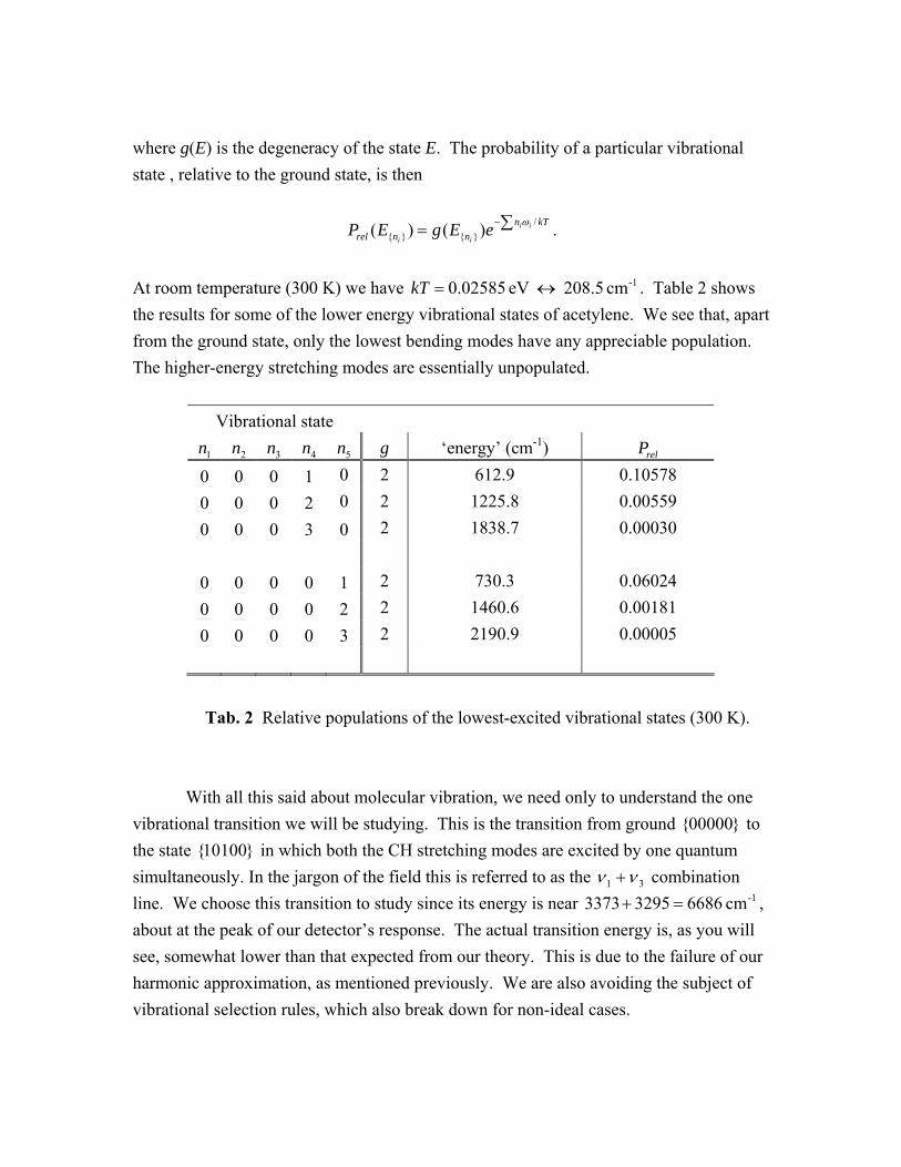
where g(E) is the degeneracy of the state E. The probability of a particular vibrational state , relative to the ground state, is then

kTnnnrel

ii

iieEgEP /

}{}{ )()( ω∑= − .

At room temperature (300 K) we have -1cm 208.5 eV 02585.0 ↔=kT . Table 2 shows the results for some of the lower energy vibrational states of acetylene. We see that, apart from the ground state, only the lowest bending modes have any appreciable population. The higher-energy stretching modes are essentially unpopulated.

Vibrational state

1n 2n 3n 4n 5n g ‘energy’ (cm-1) relP 0 0 0 1 0 2 612.9 0.10578 0 0 0 2 0 2 1225.8 0.00559 0 0 0 3 0 2 1838.7 0.00030 0 0 0 0 1 2 730.3 0.06024 0 0 0 0 2 2 1460.6 0.00181 0 0 0 0 3 2 2190.9 0.00005

Tab. 2 Relative populations of the lowest-excited vibrational states (300 K).

With all this said about molecular vibration, we need only to understand the one

vibrational transition we will be studying. This is the transition from ground }00000{ to the state }10100{ in which both the CH stretching modes are excited by one quantum simultaneously. In the jargon of the field this is referred to as the 31 νν + combination line. We choose this transition to study since its energy is near -1cm 668632953373 =+ , about at the peak of our detector’s response. The actual transition energy is, as you will see, somewhat lower than that expected from our theory. This is due to the failure of our harmonic approximation, as mentioned previously. We are also avoiding the subject of vibrational selection rules, which also break down for non-ideal cases.

3. Rotation motion

Finally, we investigate the nature of the rotational part of the wave function rotψ .

In keeping with our separation-of-variables scheme, we assume the molecule to be in some specific electronic and vibrational state. Because rotation is so much slower than vibration, we approximate the molecule to be in some averaged, fixed configuration iR (dependent on the particular vibrational state the molecule is in).

Since we’re dealing with linear acetylene, excited only in its stretching modes, the problem of rotational motion is equivalent to that of a diatomic molecule: We need only consider rotation about the center of mass perpendicular to the molecular axis. The total energy is all kinetic ( 2

21 ωIKrot = )4. Since the molecular angular momentum is just

ωL I= the rotational Hamiltonian is

2

21 LI

Hrot = .

We immediately know the eigenstates: they are the spherical harmonics MJY , .

Each rotational eigenstate (quantum number J) thus has energy

)1(2

)(2

+= JJI

JE , …,2,1,0=J

and is )12( +J -fold degenerate due to the possible projections MLz = with ( JJM +−= ,,… ).

Furthermore, each eigenstate has a specific symmetry with respect to a coordinate reflection

)()1()( ,, Ω−=Ω− MJJ

MJ YY , so that states of even J have even parity, and of odd J have odd parity. This symmetry will turn out to important: an inversion Ω−→Ω in the rotational coordinates is equivalent to exchanging one carbon nuclei with the other, and similarly for the hydrogen nuclei. 4 Here, I is the moment of inertia about the CM and now ω denotes angular velocity!

That’s all we need to know, however it’s worth pointing out that I will actually increase with J (a non-rigid rotor) which produces a small additional energy proportional to 2)]1([ +JJ . We’ll ignore this, and any other higher-order effects. Let’s estimate the energy coefficient of the rotational states of acetylene. To do so we first need to calculate the moment of inertia

)(2 22HHCC rMrMI +×= .

The radii of the carbon and hydrogen nuclei (relative to the CM) are easily established from the bond lengths of Fig. 3: m 1060.0 10−×≈Cr and m 1066.1 10−×≈Hr . For the masses, we know that u 0.12=CM and u 0.1=HM , where the atomic mass unit is

kg 1066.1u 1 27−×= . As one might expect, the result is pretty small

246 mkg 1035.2 −×≈I . With this result, the rotational energy constant is then

1-4232

cm 19.1 eV 1048.1 J 1036.22

↔×=×≈ −−

I.

We see that, unlike the vibrational energies, the rotational energies are much less than kT at room temperature. The probability of encountering an acetylene molecule in an excited rotational state is therefore large, and our experiment will give a direct view of how these probabilities are distributed. 5. Ro-vibrational spectra. Consider a transition in which a molecule in a lower ‘ro-vibrational’ state absorbs a photon and is excited to a higher state. The total wave function undergoes a change characterized by the change in quantum numbers

JnJn ii ′′→ }{}{ . The transition energy is just the difference in energies of the two states:

)1(2

)1(2

22

}{,}{, +−+′′′

+−= ′ JJI

JJI

EEhii nvibnvibν .

Recall that for our 31 νν + combination line the acetylene molecule remains

linear. Thus, any dipole moment must be parallel to the molecular axis. In this case the dipole selection rules for IR absorption are 1±=ΔJ . Thus the ro-vibrational spectra divide naturally into two ‘branches’ (i.e. sets of lines) with wavenumbers: R branch: 1+=′ JJ with 0≥J .

)1()2)(1()( +−++′+= JBJJJBJ vibR σσ .

P branch: 1−=′ JJ with 1≥J .

)1()1()( +−−′+= JBJJJBJ vibP σσ . We’ve used the obvious shorthand hcEvibvib /Δ=σ and cIhB 28/ π= (and similarly for B′ ). With the definitions

BBB +′≡2 and BB −′≡δ , a little algebra allows us to rewrite the transitions in the form

1for 2)(

0for )1()1(2)(

2

2

≥+−=

≥++++=

JJJBJ

JJJBJ

vibP

vibR

δσσ

δσσ.

Since the upper (primed) state is (by definition) in a higher vibrational mode, we expect that II ≥′ and so δ is negative and probably small. We see that the R-branch forms a series of lines (ascending with J) at frequencies higher than vibσ , the P-branch at lower frequencies (descending with J), and there is no transition at vibσ . Furthermore, the spacing of adjacent lines are

.4)1()0(

1for )12(2)1()(

0for )32(2)()1(

B

JJBJJ

JJBJJ

PR

PP

RR

=−

≥+−=+−

≥++=−+

σσ

δσσ

δσσ

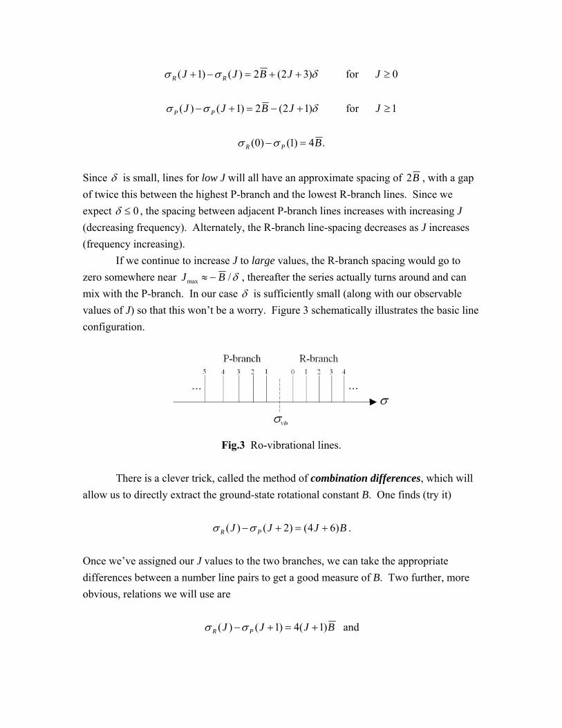
Since δ is small, lines for low J will all have an approximate spacing of B2 , with a gap of twice this between the highest P-branch and the lowest R-branch lines. Since we expect 0≤δ , the spacing between adjacent P-branch lines increases with increasing J (decreasing frequency). Alternately, the R-branch line-spacing decreases as J increases (frequency increasing).

If we continue to increase J to large values, the R-branch spacing would go to zero somewhere near δ/ max BJ −≈ , thereafter the series actually turns around and can mix with the P-branch. In our case δ is sufficiently small (along with our observable values of J) so that this won’t be a worry. Figure 3 schematically illustrates the basic line configuration.

Fig.3 Ro-vibrational lines.

There is a clever trick, called the method of combination differences, which will

allow us to directly extract the ground-state rotational constant B. One finds (try it)

BJJJ PR )64()2()( +=+−σσ .

Once we’ve assigned our J values to the two branches, we can take the appropriate differences between a number line pairs to get a good measure of B. Two further, more obvious, relations we will use are

BJJJ PR )1(4)1()( +=+−σσ and

2)1(22)1()( ++=++ JJJ vibPR δσσσ . Next, consider the intensity of the absorption lines. For the most part, these simply reflect the populations of the initial states so we can use Boltzmann statistics to predict line intensity. However, there is one more complication to consider first. This complication involves the degeneracy g(E) of our energy states and yet another degree of freedom we need to consider—nuclear spins. Acetylene is made of carbon and hydrogen. Naturally occurring carbon is almost all (98.9%) of the isotope 12C which has nuclear spin 0=s . Hydrogen 1H on the other hand has a spin 2

1=s (Deuterium 2H is very rare in nature).

The hydrogen spins on either side of the molecule have a slight interaction we can ignore, except for the fact that any interaction at all makes the total (coupled 21 ssS += ) spin states the appropriate nuclear-spin states to consider. As we all know, two spin ½ states couple to give either a singlet ( 0=S ) or a triplet ( 1=S ) total angular momentum state with 12)( += SSg degenerate eigenstates of zS . As with the rotational wave functions, these states of total nuclear spin (ns) also have a definite parity under exchange of spin coordinates:

),()1(),( 21;

112; ssss Sns

SSns ψψ +−= ,

i.e. the triplet is symmetric under coordinate interchange, and the singlet is anti-symmetric.

Now we must apply quantum mechanics at its most fundamental level. Since the electrons and hydrogen nuclei are all fermions (intrinsic spin ½) the total molecular wave function must be anti-symmetric under interchange of any pair of their coordinates. The ground electronic and vibrational states are symmetric functions, so the symmetry of the state is determined by the rotational and nuclear-spin degrees of freedom. Under interchange of the hydrogen coordinates the total wave function undergoes

ψψ JS )1()1( 1 −−→ + which must be anti-symmetric. Thus, ground molecular states of even J must have

0=S , and odd J states require 1=S . Because of the extra nuclear-spin degeneracy )(Sg odd-J lines will be about three times as intense as adjacent even-J lines. More

precisely we can write the line intensities as

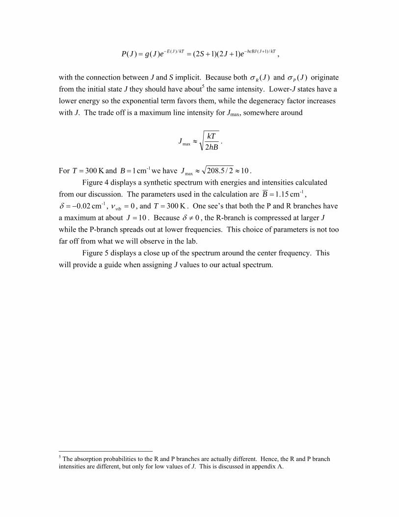
kTJhcBJkTJE eJSeJgJP /)1(/)( )12)(12()()( +−− ++== , with the connection between J and S implicit. Because both )(JRσ and )(JPσ originate from the initial state J they should have about5 the same intensity. Lower-J states have a lower energy so the exponential term favors them, while the degeneracy factor increases with J. The trade off is a maximum line intensity for Jmax, somewhere around

hBkTJ

2max ≈ .

For K 300=T and -1cm 1=B we have 102/5.208max ≈≈J .

Figure 4 displays a synthetic spectrum with energies and intensities calculated from our discussion. The parameters used in the calculation are -1cm 15.1=B ,

-1cm 02.0−=δ , 0=vibν , and K 300=T . One see’s that both the P and R branches have a maximum at about 10=J . Because 0≠δ , the R-branch is compressed at larger J while the P-branch spreads out at lower frequencies. This choice of parameters is not too far off from what we will observe in the lab.

Figure 5 displays a close up of the spectrum around the center frequency. This will provide a guide when assigning J values to our actual spectrum.

5 The absorption probabilities to the R and P branches are actually different. Hence, the R and P branch intensities are different, but only for low values of J. This is discussed in appendix A.

-100 -80 -60 -40 -20 0 20 40 60 80 100

σ (cm-1)

Fig. 4 Calculated ro-vibrational spectrum.

Fig. 5 Detail of the spectrum near the center frequency. C: PROCEEDURE You should (of course) have studied this write-up before coming to lab!

1. Acquiring data

To start, spend some time familiarizing yourself with our FTIR spectrometer: Your lab instructor will give you the basic tour and introduction to the machine. Additionally, appendix C is included as a quick reference to the MIR 8000 software. The FTIR needs to run for about an hour to stabilize, so this time can be used in practice taking low-resolution data and manipulating it with the spectral viewer. Once you’re familiar with the FTIR operation, take a ‘good’ spectrum of acetylene. A resolution of 1 cm-1 is adequate for our purposes, averaging a total of 1000 to 1500 scans. Remove the acetylene cell and take a blank spectrum with the same resolution and total number of scans. It’s a good idea to save data in several files rather than a single (see appendix C). A total scan of 1500 passes will take about 45 minutes with this resolution. Instead of surfing the web while this is going on, you can begin the analysis part of the lab by preparing some of the Excel datasheets—such as exercise III. Once both scans are completed, use the spectral viewer software to add up total acetylene and blank spectra. Divide these spectra to get an acetylene transmission spectrum and export the area of interest6 as a ‘.txt’ file. Copy this to a floppy disk and transfer to your own computer. 2. Analysis Import your text file into an Excel spreadsheet and plot the acetylene transmission data in the range around our 31 νν + combination line. Adjust the scale of the graph so you can see the first 20 or so lines of both rotational branches. At this point you need to assign J values to the lines. This is not straightforward, the oscillating background can be confused with the weak central lines. The best way is to pair up the most intense lines of the R and P branch (these will be odd J) and work inwards, using Fig. A1 as a guide. Locate the first 20 peak positions of both the P and R branches. For our purposes, it’s sufficient to simply locate the data point of a peak with maximum intensity. You can do this easily by clicking on the graph and moving the pointer from data point to data point: a box will appear with each point’s x and y values. In your excel file make

6 i.e. what is displayed currently in the spectral viewer. If you choose too wide a range the data file will be unmanageable in Excel.

columns of J, )(JPσ , and )(JRσ values. We’re now ready to extract the ro-vibrational parameters by calculating appropriate combination differences. Begin by calculating )64/()]2()( ++− JJJ PR σσ . If you’ve assigned the J values correctly these quantities should all be similar and equal to the ground-state parameter B. Compute the average and standard deviation of these values—this is our experimental value and error for B. Repeat the procedure, this time calculating )1(4/)]1()([ ++− JJJ PR σσ . This gives us an experimental value and error for 2/)( BBB ′+= . With the values of B and B , find the values and errors7 of B′ and δ. Notice that this isn’t a very accurate method for determining δ. To overcome this limitation, we use our final difference relation: Compute columns for 2)1( +J and 2/)]1()([ ++ JJ PR σσ . A plot of these quantities should give a reasonably straight line. Fitting a straight line to this data gives us vibσ (the intercept) and δ (the slope). You can do this by adding a trend line to the graph, however this gives us no idea of the error. To get the standard error in the fit parameters, use the ‘regression’ function under the excel tools/data analysis menu. Using this value and error of δ, go back and determine B′ again. For your final results, choose the best values of B, B′ , and vibσ . 3. Exercises I. From your values of B and B′ determine the moments of inertia for the ground and excited states. Since the 31 νν + combination line only excites symmetric and anti-symmetric CH stretching modes, assume the CC separation remains unchanged. Using the ground-state configuration of Fig. 3, determine the CH separation in the excited vibrational state. Recall that these ‘separations’ are the positions of the nuclei averaged over the vibrational motion. Now, in a harmonic potential, the average position is the same for all states. Convince yourself that the actual potential must be something along the lines of the potential curve of Fig. 2, i.e. opening out to larger separations. (Sketch in excited wave functions).

7 If you don’t know how to propagate errors, it’s time you should. Consult the UT Primer on the subject located on the class web site.

II. The first correction to the harmonic approximation is to include an extra term to the energy expression for a vibrational mode:

2)()( 2/12/1 +++= iiiiii nnE χωω , where the parameter iχ is called the ‘anharmonicity constant’ of the ith mode. For the Morse potential these are exact eigenvalues. Using your measured value of vibσ and the values in Table 1, what is the average

2/)( 31 χχχ += ? III. Make an excel spreadsheet that plots a synthetic ro-vibrational spectrum as in Fig. 4. As parameters, use your measured values of B and δ. Make the temperature T an adjustable parameter, and calculate lines up to at least J = 60. Don’t worry about the relative transition amplitudes discussed in appendix A. Explore how the spectrum changes with temperature. Print out spectra for T = 100, 300, and 900 K. REFERENCES FTIR: Fundamentals of Fourier Transform Infrared Spectroscopy, by B.C. Smith (CRC Press, 1996). Modern Fourier Transform Infrared Spectroscopy, by A.A. Christy, Y. Ozaki, and V.G. Gregoriou (Elsevier, 2001) [Comprehensive Analytical Chemistry vol. 35] Some introductory physics of molecules: Atoms and Molecules, by M. Weissbluth (Academic Press, 1978) Molecules and Radiation: An Introduction to Molecular Spectroscopy, by J.I. Steinfeld (The MIT Press, 1981) Advanced, including details of acetylene’s normal modes: Molecular Spectra and Molecular Structure II. Infrared and Raman spectra of Polyatomic Molecules, by G. Herzberg (Van Nostrand Co., 1945)

APPENDIX A: Relative absorption strengths.

While the ro-vibrational lines )(JRσ and )(JPσ both have intensities proportional to the population of their common initial state J, to be more precise we should also consider their absorption probabilities. These depend on whether 1+→ JJ or 1−→ JJ . The treatment of this problem rests on the algebra of angular momentum. Since this is a little more advanced and the physics non-intuitive, we’ve relegated the subject to this brief appendix where the ideas are simply outlined and results presented.

For absorption from an initial state J to another state J ′ , the transition probability is proportional to

2

,)(1)( ∑

′

′′=′→MM

MJJMJg

JJW R .

Here, we calculate the dipole probabilities of each transition MJJM ′′→ , summing over all final substates M ′ and averaging over all initial M substates. This double sum is called the line strength of the transition. Using some techniques standard in atomic physics, the summation can be resolved to an M- and M ′ -independent quantity: ‘the reduce matrix element of the renormalized spherical harmonic of rank 1’. In symbols

2)1(

)12(1)( JCJ

JJJW ′

+=′→ .

While these functions have an analytic form, all we care about is their numerical values. In particular, we want to determine the ratio of intensities of the R and P branch lines originating from the Jth ground-state rotational level.

Since the line ‘intensities’ are

)1()()( +→= JJWJPJIR and

)1()()( −→= JJWJPJIP , we see that the intensity ratio of the R-branch line to the P-branch line is simply

)1()1(

)()(

−→+→

=JJWJJW

JIJI

P

R .

With no further ado, we simply present the results:

J )(/)( JIJI PR 1 2.000 2 1.500 3 1.333 4 1.250 5 1.200 6 1.167 7 1.143 8 1.125 9 1.111 10 1.100

One sees that the effect dies off rapidly and so, except for the lowest values of J, it’s permissible to neglect the absorption line strengths as we have in Fig. 5. However, it’s the low-J region we use to identify the lines. For this purpose, we revise Fig. 5:

Fig. A1 Low-J synthetic spectra, corrected for transition strengths.

APPENDIX B: Fourier transform spectrometers.

A. Overview

With the advent of several technologies (particularly computers) Fourier-

transform spectroscopy has become a practical tool for studying the transmission properties of substances in the IR regime. Fourier-transform infrared (FTIR) spectrometers are standard items in the laboratory, used extensively for chemical analysis. In general FTIR spectroscopy is much more efficient than more traditional spectrometers based on dispersive elements such as prisms or gratings.

Instead of dispersive optics, FTIR is based on the use of an interferometer. Figure B1 below shows a block diagram outlining the spectrometer’s operation. Before looking at details, let’s consider the overall scheme of the spectrometer:

Fig. B1. FTIR operation.

A Broadband IR source, often a tungsten-halide lamp, is shone through the

sample under study. The source has a distribution of intensity over frequency )(0 νI , and after traversing the sample assumes a new distribution )()()( 0 ννν ITI ss = . The sample transmission )(νsT is our quantity of interest, related to the absorption ( TA −=1 ) and so ultimately to the sample’s photo-absorption cross section via Beer’s law.

The sample intensity is directed into the heart of the spectrometer, the interferometer. Here, as we shall see, the entire spectral range of the sample intensity is employed in the measurement. It is this use of all frequency components simultaneously which makes FTIR spectroscopy so efficient: In dispersive methods we single out a single frequency at a time, throwing away all others for that measurement.

The output of the interferometer )( xIs Δ turns out to be the Fourier transform of )(νsI . A computer is than used to invert the transform. This is accomplished using the

highly efficient fast Fourier transform (FFT) algorithm— without the FFT routine FTIR would be impractical.

The sample transmission is a combination of the transmission of the sample cell and that of the substance we are actually interested in, say XT , so that cellXs TTT ×= . To get XT one takes two measurements, one of the sample and the other of a blank cell. If you ensure that these two measurements collect the same total irradiance (e.g. same number of scans) then the substance’s transmission can be obtained by numerically dividing the two spectra )(/)()( ννν blanksX IIT = . Often this procedure is useful simply to remove the frequency variation of the source (and detector). B. How it works

Let’s now turn to the details of the interferometer. FTIRs employ some version of the basic Michelson-Morley interferometer shown in Fig. B2.

Fig. B2. Michelson-Morley interferometer. Consider a plane wave of amplitude 0E and frequency ν entering the interferometer from the left. The wave propagates along a linear path as

)2cos(),( tkxEtxE s πν−= , where x is the distance traveled and the wavevector ck /2/2 πνλπ == 8. The average intensity of this wave is 2

ss EI = . When the wave reaches the beam splitter it’s separated into two waves each with ½ the original amplitude; one is transmitted (blue) and the other (red) is reflected9. The reflected wave travels upward until it’s reflected by the fixed mirror, finally traveling down through the beam splitter and into the detector. The transmitted wave travels on to the right where it’s reflected back by the movable mirror, then back off the beam splitter where it finally recombines with the first wave at the detector. The position

xΔ of the movable mirror is measured with respect to the point 0x , the distance at which both mirrors are equidistant from the beam splitter. Consider the mirror set at some position xΔ . The amplitude of the recombined wave at the detector (D) is

[ ])22cos()2cos(2

),( txkkDtkDEtDE s πνπν −Δ++−= ,

the second wave having traveled an extra distance xΔ2 . This distance is called the optical path difference (OPD) which we denote as , and can be either positive or negative. The sum of the two oscillatory terms must itself oscillate at the same frequency, so we can write in general that

).cos()cos()cos( tAtt ωδωβωα +=+++ Since we are interested only in the average intensity of the recombined wave, which is what the detector responds to, all we need find is 2A . This is easily accomplished by representing the cosines as phasors and then employing trigonometry to solve the vector sum. The result is

)cos(222 αβ −+=A .

8 Note that (the magnitude of) the wavevector = 2π wavenumber, like ω = 2π ν. Also, c and λ are really not the vacuum values, but those within the media (i.e. air) filling the spectrometer. 9 For simplicity, we ignore any phase changes associated with reflectance etc. – real FTIRs include extra optical elements to compensate for these effects.

The average intensity at the detector is therefore

[ ])cos(12

kII sD += .

Now, consider a broadband spectrum of waves entering the interferometer. The average intensity of each such wave is )(kIs . We use an incoherent source (i.e. an incandescent lamp), which means there is no steady phase relationship between waves of different frequency. If this is so, then the detector responds to the (incoherent) sum of intensities of the individual waves, so that for a given mirror displacement the total detected intensity is

∫∞

+=0

)cos()(21

21)( dkkkIII sTD ,

where the total intensity is

)0()(0

DsT IdkkII == ∫∞

.

Hence, if we scan the mirror back and forth around the zero position we are

essentially recording the Fourier (cosine) transform of the incident intensity distribution. The wavenuumber k and the OPD naturally arise as a complimentary pair of variables for the transformation. FTIR spectra are usually output as a function of k in cm-1.

A small HeNe laser is used to accurately measure : The HeNe beam is simultaneously passed through the interferometer and monitored with its own detector. Counting interference fringes as the mirror moves locates its position to within a laser wavelength ( μm6.0nm633 ≈ ).

Note that when 0= waves of all frequencies add constructively, but for larger the integrand oscillates with k and so the integral becomes small. The transformed data

)(DI is therefore strongly peaked about 0= , and this peak is often referred to as a center burst. However, the small-amplitude data away from the center burst provides most of the information needed to reconstruct the spectrum.

Figure B3 shows a typical center-burst plot. The native data plotted is something proportional to

)0()(2)( DD IIf −= .

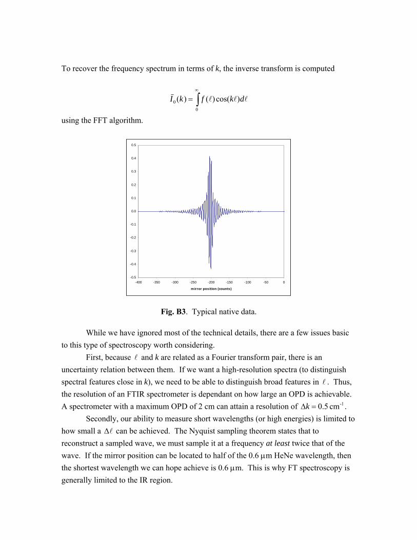
To recover the frequency spectrum in terms of k, the inverse transform is computed

∫∞

=0

0 )cos()()( dkfkI

using the FFT algorithm.

-0.5

-0.4

-0.3

-0.2

-0.1

0.0

0.1

0.2

0.3

0.4

0.5

-400 -350 -300 -250 -200 -150 -100 -50 0

mirror position (counts)

Fig. B3. Typical native data.

While we have ignored most of the technical details, there are a few issues basic to this type of spectroscopy worth considering.

First, because and k are related as a Fourier transform pair, there is an uncertainty relation between them. If we want a high-resolution spectra (to distinguish spectral features close in k), we need to be able to distinguish broad features in . Thus, the resolution of an FTIR spectrometer is dependant on how large an OPD is achievable. A spectrometer with a maximum OPD of 2 cm can attain a resolution of -1cm 0.5 =Δk .

Secondly, our ability to measure short wavelengths (or high energies) is limited to how small a Δ can be achieved. The Nyquist sampling theorem states that to reconstruct a sampled wave, we must sample it at a frequency at least twice that of the wave. If the mirror position can be located to half of the 0.6 μm HeNe wavelength, then the shortest wavelength we can hope achieve is 0.6 μm. This is why FT spectroscopy is generally limited to the IR region.

APPENDIX C: MIRMAT 8000 FTIR Here’s a pictorial outline of using the MIRMAT software. We will use the program for two separate tasks: A) acquiring and storing an FTIR spectrum and B) manipulating these spectra. The program is a little puzzling with some (what I think are) bugs. A) Acquiring data Make sure the FTIR power is on. On the computer desktop, click on the MIRMAT 8000 icon to launch the program. The opening screen will appear:

Opening screen Double click on the MIRMAT start option. A box will appear asking if you want to initialize the instrument. Click yes. The setup screen then appears. There are only three settings we need monkey with: Detector: Choose InGaAsP. Resolution: 64 cm-1 is fast for practice, and 1 cm-1 is enough for resolving the H2C2 lines. Saving Method: This determines how the data is stored. If you are just fooling around, leave the setting at ‘Prompt Me’. Otherwise choose ‘Loop Mode’. A box will appear telling you it has reset the trigger mode.

Setup screen Once, you’ve made your choices, click on accept which opens the data screen:

Data screen If you are fooling around (prompt mode) just leave all the settings and click ‘fresh start’.

If you are acquiring data for real (loop mode) you need to give some information: In this mode the spectrometer adds each scan to the last—up to the number specified by ‘Coadd# of scans’ (in this example 512 scans). This result is then saved to file in a binary format (.mat). Then the process is repeated. The Number of Loops can be adjusted to control this (here 3 loops). Each of these files will be placed in the directory you choose (here in C:\BRAD). The directory must already exist. (it’s easiest to make

your own in the root directory). Each loop of data will be stored with the File Name you specify, appended by the loop number, i.e. here C2H2_1.mat, C2H2_2.mat, and C2H2_3.mat. If you want, you can also fill in the comment lines, however this won’t be of much use to us. When you are ready to scan, click on ‘Fresh Start’. The program will begin acquiring data:

Fast acquisition screen In the loop mode, the actual interferometer data is displayed in real time, but the Fourier transformed spectrum is not. In this example we’ve already taken 14 scans of the first (0th) loop. If at any time you want to look at the spectrum acquired, you must click the interrupt button which halts the acquisition. If you then click ‘auto scale Y’ you should see something like

Halted acquisition

To continue taking data click ‘continue’. If you want to explore the spectrum in more detail, once you have interrupted the acquisition, click on the lower SPV (spectral viewer) button:

Spectral viewer Within the spectral viewer you can look at various portions of the spectrum, change units and manipulate data. (Next section). To continue taking data, click ‘close’ and then ‘continue’ on the acquisition screen. When the final loop finishes, the program idles and you can exit. Notice the absorption band around 7000 cm-1 in the above example. This is due to water vapor—the spectrum here is a blank. B) Manipulating spectra. Once you’ve collected data files you will need to manipulate them in several ways. This is accomplished using the ‘spectral viewer’. The spectral viewer allows you to read in .mat format spectrum files, store them in various temporary registers, perform mathematical functions on individual spectra (such as taking the logrithim) and on pairs of spectra (such as adding and dividing). To get good data, we will want to add up separate data files, and to get rid of the source/detector variations we will want to divide the total acetylene spectrum by the blank spectrum.

From the MIRMAT opening screen, click on ‘SPViewer’. The opening screen will appear showing a generic center burst. To load a previously-saved .mat file, click on the Load button. A box will appear, and you can choose the file you want to load (the browse button is easiest).

A primitive .mat file contains a lot of information. We want the plot of the resulting spectrum verses wavenumber.

Opening screen

Loading a file to view To get this data, we need to tell SPV what to plot. To do so, click on wav (for wavenumber) in the file contents box, then on the arrow button directing the data ‘into’ the x axis. Then similarly direct the spec data into the y axis. If you are dealing with .mat files that have been manipulated and resaved, the choices of data to plot will be x and y instead of wav and spec. Once you are ready click OK. You will then see the data displayed as:

Pushing to stack A There are 6 memory stacks or registers in which spectra can be stored. The above figure shows the data being pushed into stack A; simply pull down the Mem Stack selection arrow and click on the stack you want. Now you are free to load another file without loosing the current data. The screen below shows the situation in which there are two stacks loaded, A and B: You can tell which stacks are loaded from the buttons in the lower left corner—stacks that have something in them are in bold face type. Pushing on any of these buttons displays the contents.

Summing two spectra

Now, to operate on the stored data click on the Math button. The left hand window will open. Important to us is the Function(A?B) button. push it and the lower window opens. This window allows us to perform operations on two spectra, saving the

result in another stack. In this example we’re adding spectrum A to spectrum B and saving the result to stack C. Note here the notch near 6500 cm-1, which is due to acetylene absorption. Now, when you have something you want to work with you need to export it as a text file. We need to make this file as small as possible, so use the x-axis boxes to reduce increase the scale around your area of interest. In the example below, we’re looking at the reduced range of 6000 to 8000 cm-1. (You can now see the R and P branches of the acetylene transitions.)

For your transmission data, only export data region that includes the R and P branches – there are a lot of data points here, especially using high resolution. To export what is displayed as a text file, click Export. A typical file-handling window will open and you can enter a file name. The only trick is that you are not offered a .txt choice of file type. However, if you simply include the extension with the file name the program knows what to do. For more information (but not much) you can consult the MIR 8000 manual.