· Informix Roadmap. 2Q17. 3Q17. 4Q17. Stretch. Delight the Customer. Cloud. IoT. Backup to Object...
335
Informix Update – New Features & Partnerships IBM Data Server Day – Stockholm May 2017 Scott Pickett WW Informix Technical Sales For questions about this presentation contact: [email protected] © 2017 IBM Corporation
Transcript of · Informix Roadmap. 2Q17. 3Q17. 4Q17. Stretch. Delight the Customer. Cloud. IoT. Backup to Object...

Informix Update – New Features & PartnershipsIBM Data Server Day – Stockholm May 2017
Scott Pickett WW Informix Technical SalesFor questions about this presentation contact: [email protected]
© 2017 IBM Corporation

Agenda
Informix Roadmap A New Partnership 12.10.xC8 – Highlights – released 12/01/2016 12.10.xC7 – Highlights – released 06/23/2016 12.10.xC6 – Highlights – released 11/24/2015 12.10.xC5 – Highlights – released 03/24/2015 Appendices
© 2017 IBM Corporation2

Informix Roadmap
© 2017 IBM Corporation
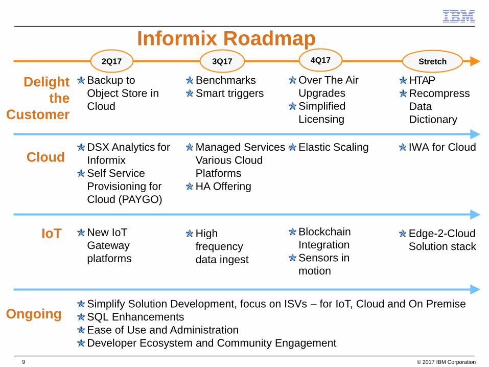
Informix Roadmap2Q17 3Q17 4Q17 Stretch
Delight the
Customer
Cloud
IoT
Backup to Object Store in Cloud
DSX Analytics for InformixSelf Service Provisioning for Cloud (PAYGO))
BenchmarksSmart triggers
Over The Air UpgradesSimplified Licensing
Managed Services –Various Cloud Platforms HA Offering
BlockchainIntegrationSensors in motion
Elastic Scaling
Simplify Solution Development, focus on ISVs – for IoT, Cloud and On PremiseSQL EnhancementsEase of Use and AdministrationDeveloper Ecosystem and Community Engagement
Ongoing
HTAPRecompress Data Dictionary
Edge-2-Cloud Solution stack
IWA for Cloud
New IoTGateway platforms
High frequency data ingest
© 2017 IBM Corporation9

IBM Informix & HCL Partnership
© 2017 IBM Corporation

News for Informix Customers - HCL Global Partnership
World-class partner taking responsibility for Informix Development & Support Richer roadmap, delivered sooner
Co-marketing support
Co-tech sales support
IOT expertise
Capture IOT whitespace
© 2017 IBM Corporation11

IBM and HCL Relationship to Expand Informix
HCL is now responsible for Informix Development and Support– Full Informix development and support (L2,L3) transfers to HCL as part of the
larger HCL development organization. • HCL employs more than 100,000 employees worldwide.
– Seamless transition, ensuring Informix expertise is maintained.– License agreement provides the right to develop Informix only
• This is not a sale of the product and all that goes with it.
No change to Informix client relationship and processes (e.g., sales relationships, passport advantage, quotes, invoicing and payments)
IBM is responsible for Informix Sales, Tech Sales, Marketing, Lab Services and L1 Support – In addition, HCL will help with co-marketing and tech sales support
HCL and IBM will co-manage the Informix Customer Roadmap
Development is underway and xC9 is due at the end of this quarter.© 2017 IBM Corporation12

Informix Products Affected
Informix Server & CSDK Informix Connect Runtime Informix Warehouse Accelerator (IWA) Informix 4GL Informix SQL Informix on Cloud
© 2017 IBM Corporation13

About HCL
REST OF WORLD
EUROPE
AMERICAS
MANUFACTURING
FINANCIAL SERVICES
LIFESCIENCES & HEALTHCARE
PUBLIC SERVICES
TELECOM, MEDIA, PUBLISHING & ENTERTAINMENT
RETAIL AND CPG
OTHERS
32%
10%
9%
10%
1%
26%
12% APPLICATION SERVICES
40.9%
INFRASTRUCTURE SERVICES
ENGINEERING ANDRESEARCH SERVICES
10%
30%
60%
Vertical MixREVENUES
Service MixREVENUES
Geo MixREVENUES
PEOPLE & INDUSTRIES REVENUE & SERVICE LINES GLOBAL COVERAGE
111,000+31
COUNTRIES7.1
BILLION USD
36%
40%
19%
BUSINESS SERVICES
14.4%
5%
© 2017 IBM Corporation14

Key Points These offerings are strategically important to IBM. IBM recognizes the need to increase capacity and to innovate in
these areas. IBM intends to deliver additional capabilities to our clients. This partnership has been made to secure the long-term success of
our DevOps solution. IBM is expanding the existing partnership for 15+ years with HCL to
accelerate the product roadmap innovation and extend these products to IOT.
IBM – HCL Partnership (1)
© 2017 IBM Corporation15

Key Points IBM will continue to sell these products as it does today
– No change to contracts.– Sales contact is still with IBM. – Executive, technical and advocate relationships are unchanged.– IBM will continue to be the first point of contact for support and work with HCL
who will provide advanced support (L2, L3) and development.– Support management will be through the PMR process, you will not be
required to manage the transition in support between IBM and HCL.– IBM license, pricing, sales and support channels are unchanged.– Our client commitments remain the same.
IBM – HCL Partnership (2)
© 2017 IBM Corporation16

More Information
From Matthias Funke, IBM: https://www.linkedin.com/pulse/explaining-new-ibm-hcl-partnership-
informixand-why-good-funke?trk=v-feed&lipi=urn%3Ali%3Apage%3Ad_flagship3_feed%3B2wUdozQhS66GTZQO9pliQQ%3D%3D
From Daniel Hernandez, IBM: http://www.iiug.org/en/2017/04/17/ibm-and-hcl-strategic-partnership-
to-jointly-develop-and-market-ibm-informix/
© 2017 IBM Corporation17

HCL VP of Development - Darren Oberst - Statement
© 2017 IBM Corporation18

International Informix User Group President Comments
https://www.linkedin.com/pulse/explaining-new-ibm-hcl-partnership-informixand-why-good-funke
© 2017 IBM Corporation19

Contacts – WW Informix – IBM & HCL Partnership IBM Informix Technical Sales
– Scott Pickett
IBM Informix, Cloud & DB2 Sales – Tomas Escobar
IBM Partner & Embed Sales– Joseph Costabile
IBM Director Core Database & Data Warehouse Offering Mgmt & Strategy– Matthias Funke
IBM VP, Hybrid Platform Development and Client Success, Hybrid Cloud – Albert Martin
HCL Informix Sales Director– Marcelo Cabane
HCL Informix Offering Mgmt. – Karen Qualley
HCL Informix Product Development– Pradeep Muthalpuredathe
HCL Informix Tech Support Mgr.– Michael O’Brien
HCL Vice President of Sales, Lab Services and Client Advocacy– Doug Snadecki
HCL Development Vice President– Darren Oberst
© 2017 IBM Corporation20

Informix 12.10.xC8 – New Features
© 2017 IBM Corporation

Agenda Encryption at Rest Consistent sharded insert, update, and delete operations List Enterprise Replication definition commands Complex text search with regular expressions Suspend validation of check constraints Advanced time series analytics
© 2017 IBM Corporation22

Encryption at Rest (EAR)
© 2017 IBM Corporation

poiunponorwborwbbgr
Cvvebvfrbnnym,.i/.oi/o/.,utnjtrrewfevhj64u79i0-[-htjyuyoiuomffddbcxbvdgdcnbcncncmcds;x.vcmbvmglknbmvfmvfvjveijveevvvvovovvovovdvodvdvonvdovndvodnvovdnvovvovnfdovdnvodnvovnvodnvdovdnvovnvodnvovnvovndovnvoewjfdpvke[v[rjfoegfjerijeiejveiviewjfijveqivjfieivieqnveivenveinvevinmevienviveviveivjviejveivjviejveivjviejvijeviejviejeijfuyu43y6364387498h095h09=ke0vj0bijb0ije0ijv0ikjv0iv oikjv0ivjvvkjv0jk0idekv0ikjbve0ibvkj0ekfkif0-if0-fi0-ffif0-ngngngngngnif0oifiefief0kif0ev0kibv0ekjekjbv0jjkbjbjbjjbjbjbjbbjbjbjbjbbjbjbjbjbjbjjbjbjbjbjbjbjbjbjjbjbjbjbjbjbbjbjbjbjbbjbjbjbbbjbjbjbjbbjbjbjbjbjbjbjbjbjbjbjbbjbjjbjbjbjbjbjjbjbjbjbjbjbjbj9’/njtvgfeds2q2`fr42hy,mmrernbygmjkpo?0[0hhj6jj7km7km7,.,.9l9l;l9ll98;l98liu,miu,mumn443r32vrebrref3vg nbtrggr nrgr gigo ntrnbrtnytnnby.i;l8loijarshagnmy,uil/.fbt[5lkpbkrpb,mg,br;,brb,rb,rl,,bLnb, n,n,brw,brw,rw,rb[r,.brwl,brwNbl,r n, nbrwB,w ,n[ ,n[N,tr[nn[,rn [rhbrhbjbkjbfbfkbgf b kbgbbg bg bg bbbgb b bgbgbbgbb bg;.,./?????????????????????????????????????????????????
© 2017 IBM Corporation25
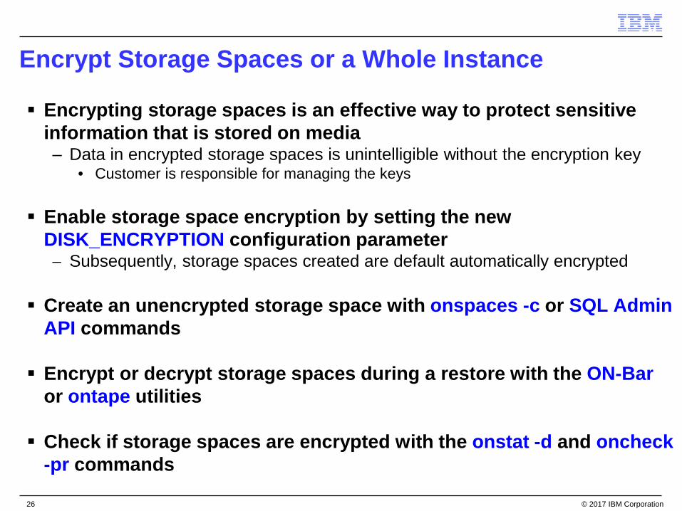
Encrypt Storage Spaces or a Whole Instance
Encrypting storage spaces is an effective way to protect sensitive information that is stored on media‒ Data in encrypted storage spaces is unintelligible without the encryption key
• Customer is responsible for managing the keys
Enable storage space encryption by setting the new DISK_ENCRYPTION configuration parameter− Subsequently, storage spaces created are default automatically encrypted
Create an unencrypted storage space with onspaces -c or SQL Admin API commands
Encrypt or decrypt storage spaces during a restore with the ON-Baror ontape utilities
Check if storage spaces are encrypted with the onstat -d and oncheck-pr commands
© 2017 IBM Corporation26

DISK_ENCRYPTION configuration parameter
Controls the encryption of storage spaces ‒ Not set by default‒ Not dynamic
Once enabled, any storage spaces created are encrypted by default− Previously created storage spaces will not be encrypted.
− Can be encrypted via backup/restore
Set the encryption file names, cipher to use, the configuration parameter to enable storage space encryption
When storage space encryption is enabled, you can restore a storage space as encrypted or unencrypted, regardless of whether the space was encrypted at the time of the back up
Backup data and Restore data are encrypted/decrypted via the BACKUP_FILTER and RESTORE_FILTER parameter
© 2017 IBM Corporation27

DISK_ENCRYPTION configuration parameter
>>-DISK_ENCRYPTION--keystore--=--keystore_name------------------>
>--+--------------------------+---------------------------------> '-,--cipher--=--+-aes128-+-' +-aes192-+ '-aes256-'
>--+---------------------------------------+------------------->< '-,--rollfwd_create_dbs--=--+-encrypt-+-' '-decrypt-'
© 2017 IBM Corporation28

DISK_ENCRYPTION configuration parameter
keystore − The keystore specifies the name of the keystore and stash file names. − The files are created in the INFORMIXDIR/etc directory:
keystore.p12− The keystore file that contains the security certificates
keystore.sth− The stash file that contains the encryption password
You must manually back up (via operating system backup) the keystore and password stash files− Files are not backed up when ON-Bar or ontape backs up
© 2017 IBM Corporation29

DISK_ENCRYPTION configuration parameter
cipher − The encryption cipher:
• aes128 - Default. Advanced Encryption Standard cipher with 128-bit keys• aes192 - Advanced Encryption Standard cipher with 192-bit keys• aes256 - Advanced Encryption Standard cipher with 256-bit keys
rollfwd_create_dbs− Whether to encrypt a storage space created by the rolling forward of the logical
log during a restore:• encrypt - Encrypt the newly created storage space• decrypt - Do not encrypt the newly created storage space
− Default, storage spaces that are created by the rolling forward of the logical log have the same encryption state as the original storage space
© 2017 IBM Corporation30

onspaces Unencrypted Option
To create an unencrypted storage space, even if DISK_ENCRYPTION is turned on:− onspaces –c –d unencrypted_space –p /usr/storage/unencrypted_dbs1 –
o 0 –s 2000000 –k 2 –u
– execute function task("create unencrypted dbspace…
– execute function task("create unencrypted blobspace…
– etc…
© 2017 IBM Corporation31

Quick Start (1)
Set DISK_ENCRYPTION in the instance configuration file: DISK_ENCRYPTION keystore=jc_keystore oninit –ivy …..
© 2017 IBM Corporation33

Quick start (2) – Message Log File ... ... Initializing Dictionary Cache and SPL Routine Cache...succeeded Initializing
encryption-at-rest if necessary...succeeded Initializing encryption-at-rest structures (part 1)...succeeded Bringing up ADM VP...succeeded
Creating VP classes...succeeded Forking main_loop thread...succeeded Initializing DR structures...succeeded
Forking 1 'ipcshm' listener threads...succeeded Starting tracing...succeeded Initializing 1 flushers...succeeded Clearing encrypted root chunk 1 before initialization... 25% done. 50% done. 75% done. 100% done. Initializing encryption-at-rest structures (part 2)...succeeded Initializing log/checkpoint information...succeeded ... ...
© 2017 IBM Corporation34

Quick Start (3) – Instance Results (default)
Initially, a new instance with one chunk, encrypted using the default cypher (aes128)– This will be key1 on dbspace1 (rootdbs) for this instance
Installation locations, keystore and stash files:– $INFORMIXDIR/etc/jc_keystore.p12 – $INFORMIXDIR/etc/jc_keystore.sth
Each space in an instance uses a different encryption key– Keys 2-2047 are derived from Key 1 at run-time and never stored anywhere on
disk
© 2017 IBM Corporation35

What’s in the Key Store File and Stash Files?
The Key Store file ($INFORMIXDIR/etc/<keystore name>.p12) contains a single encryption key, which is used only for ROOTDBS (Dbspace 1).– Key Store file is encrypted– To decrypt the Key Store file, the server needs the Master Key
The Master Key is stored in a stash file– ($INFORMIXDIR/etc/<keystore name>.sth)– The stash file is encrypted. – The server knows how to read it only because IBM GSKit knows how to read it.
• gskit is installed with Informix initially• See Appendix E for more details
Best practice is to store encrypted chunks on a separate disk from $INFORMIXDIR
Users are expected to back up $INFORMIXDIR with some regularity
© 2017 IBM Corporation36

What’s in memory
Pages in the buffer pool are not encrypted
Decryption happens during the read from disk, at a low level in the I/O code
Encryption happens at the same low level during a write
onstat -g dmp will display decrypted data
Shared memory dump files will contain decrypted data, but not encryption keys
© 2017 IBM Corporation37

Encryption and Replication
Encryption on a secondary is entirely independent of encryption on a primary
A primary may be encrypted while a secondary is not, and vice-versa
A different set of spaces may be encrypted in a primary vs. a secondary
An SDS secondary must use exactly the same encryption keys as used on the primary:– When a shared-disk secondary is first created for an encrypted primary, the
primary's keystore file is automatically copied to the secondary's $INFORMIXDIR/etc directory
– File is then encrypted with a master key stored in the stash file
© 2017 IBM Corporation38

ontape/onbar – Changing Encryption During Restores
If storage space encryption is enabled, storage spaces are restored with the same encryption state as during the back up, by default− Can specify to restore storage spaces as encrypted or unencrypted
The encryption state of storage spaces on disk does not affect the encryption state of backups− Storage spaces that are encrypted on disk are unencrypted during a backup
• To encrypt backed up storage spaces, set the BACKUP_FILTER configuration parameter to the name of an encryption utility
• When you restore a storage space that was encrypted on disk before its backup, the storage space is encrypted during the restore, unless you specify to restore the space as unencrypted
• Similarly, you can restore a storage space that was not encrypted on disk by specifying to encrypt the space during the restore
© 2017 IBM Corporation39

ontape/onbar – Changing Encryption During Restores
The following shows ways you can encrypt and decrypt storage spaces during a physical restore with the ON-Bar or ontape utilities when storage space encryption is enabled:
Task – Encrypt or Decrypt ….. MethodAll existing storage spaces Full restore with the -encrypt or -decrypt option.
Set/unset DISK_ENCRYPTIONCritical storage spaces Cold restore with the -encrypt or -decrypt option
and specify the spaces with the -D option.
Some non-critical storage spaces Warm restore with the -encrypt or -decrypt option and specify the spaces with the -D option.
All storage spaces for a tenant database Tenant restore with the onbar -T command and include the -encrypt or -decrypt option.
Storage spaces created by a roll-forward of logical logs
Include rollfwd_create_dbs=encrypt or rollfwd_create_dbs=decrypt option on the DISK_ENCRYPTION parameter value.
© 2017 IBM Corporation40

ontape/onbar – Changing Encryption During Restores
The -encrypt or -decrypt arguments to onbar or ontape apply to a physical restore only: – The server can't use them for the logical restore
Decrypt an entire instance but still enable encryption at rest by setting DISK_ENCRYPTION and perform a cold restore using the -decrypt argument:– ontape -r -decrypt– onbar -r -decrypt
During a rollforward, spaces may be re-created– Assuming Encryption at Rest is enabled, by default they will be created with the
same encryption status they were given originally
This default can be overridden by adding rollfwd_create_dbs to the DISK_ENCRYPTION setting, as in:– DISK_ENCRYPTION keystore=jc_keystore,rollfwd_create_dbs=encrypt– DISK_ENCRYPTION
keystore=jc_keystore,rollfwd_create_dbs=decrypt© 2017 IBM Corporation41

Encryption and Restores
During an external restore, storage spaces are restored to the same encryption state as during the backup‒ Encryption state of storage spaces cannot change during an external restore
When storage space encryption is not enabled, you see the following:− Encrypting storage spaces during a restore with the -encrypt option, restore
fails− Restoring encrypted storage spaces, storage spaces are restored as
unencrypted
Encrypt all existing storage spaces during a whole-system restore:− onbar -r -encrypt -w
Encrypt two storage spaces during a physical restore:− ontape -p -encrypt -D dbspace1 dbspace2
Decrypt all storage spaces that belong to a tenant database:− onbar -T tenant1 -decrypt -t "08-08-2016 00:00:00"
© 2017 IBM Corporation42

How Can I Tell Whether Encryption at Rest Is Enabled?
oncheck– oncheck -pr | head -15– oncheck –pr | grep rest
select from sysmaster:sysshmhdr
– select value from sysshmhdr where name = "sh_disk_encryption"; Look for the message "Encryption-at-rest is enabled using cipher" in
the message log file onstat -g dmp
– onstat -g dmp <rhead addr> rhead_t | grep sh_disk_encryption
© 2017 IBM Corporation43

Overwriting the Key Store and Stash Files
Each instance has its own key store and stash file.
Instances cannot share these files, but stored in a directory that may be shared– Instances that share an $INFORMIXDIR must use different key store names in
their DISK_ENCRYPTION settings.
We attempt to prevent clobbering of these files by insisting that FULL_DISK_INIT is set before they can be overwritten.
With encryption enabled, the key store and stash files will be overwritten under the following conditions:– oninit -i– Cold restore– Clone creation via ifxclone.
© 2017 IBM Corporation44

Change the Storage Space Encryption Key
master_key reset argument: (SQL administration API)
Use the master_key reset argument with the admin() or task() function to change the master key for storage space encryption– When encryption is first established, a key is automatically generated and
stored encrypted in the stash file. – User supplied master key of 32 bytes maximum encrypts the keystore for
storage space encryption.• Users informix or root only may change at any time• Stores the new encrypted key in the stash file• Accepts no argument, in which case a random master key is generated.
Make sure you write it down ……….. Do you know random ?
– execute function task(“master key reset”,”new master key, hopefully not”);
© 2017 IBM Corporation45

Caveats
You have to find somewhere to store your keys ……– Future Release
Presently, backup data is not encrypted, use BACKUP_FILTER and RESTORE_FILTER– Future Release
Don’t forget your keys ………– Fortunately, since backups are not encrypted yet, you can restore the storage
spaces unencrypted.
Use of ifxclone on an existing instance
© 2017 IBM Corporation46

Questions?
© 2017 IBM Corporation47

List Enterprise Replication Definition Commands
Customers can print a list of successful commands run to define a replication server, replicates, replicate sets, templates, or grids with the new cdr list catalog command.
Use this list of commands to easily duplicate a system for troubleshooting or moving a test system into production.
cdr list catalog− Lists the commands that created the specified replication objects− Options:
Long Form Short Form Meaning--all -a Lists all definition commands. Default.--grids -g Lists cdr create grid commands.--quiet -q Lists the commands without headings.--realizetemplates -z Lists cdr realize template commands.--replicates -r Lists cdr define replicate commands.--replicatesets -e Lists cdr define replicateset commands.--servers -s Lists cdr define server commands.--templates -t Lists cdr define template commands.
© 2017 IBM Corporation56

cdr list catalog
List the define server commands
Template realization
© 2017 IBM Corporation57

Regular Expression SQL Searches (regex)
© 2017 IBM Corporation

Complex Text Search with Regular Expressions (regex)
For SQL commands:− Search for and replace text strings with regular expressions in SQL statements. − Regular expressions combine literal characters and metacharacters to define
the search and replace criteria.
Run the functions from the new Informix regex extension to find matches to strings, replace strings, and split strings into substrings.
• Specify case-sensitive or case-insensitive searching.• Search single-byte character sets or UTF-8 character sets.
For MongoDB commands:− The JSON wire listener now supports searching with regular expressions with
the $regex operator in MongoDB commands.
© 2017 IBM Corporation60

Complex Text Search with Regular Expressions (regex)
Requirements and Restrictions:− Use basic or extended regular expressions, with case sensitivity or case
insensitivity • Neither expression type allows searching for a null character
− Extended regular expressions support more search and replace options than basic regular expressions
− Database server requirement• The Scheduler must be running
When you run regex functions, a message that the function is not found is returned if the scheduler is not running.
• Default sbspace required to return a CLOB value when you replace strings and to replace text in a CLOB value with the regex_replace function
− Database requirements• A non-ANSI logging database
If you attempt to use a regex function in an unlogged or ANSI database, the message “DataBlade registration failed” is printed in the database server message log
− Data type support• To use regex pattern matching, you must provide the text data as a CHAR,
LVARCHAR, NCHAR, NVARCHAR, VARCHAR, or CLOB data type.
© 2017 IBM Corporation61

Complex Text Search with Regular Expressions (regex)
Requirements and Restrictions (cont’d):− Locales and languages support
• Regex queries can use single-byte character locales and UTF-8 based locales.• If UTF-8 character encoding is used, including the Chinese GB18030-2000 code set,
you must set the GL_USEGLU environment variable before you create the database.− Query restrictions
• Regex functions do not inherently use any database indexes. If there is something else that can use an index in the statement …….
Metacharacters:− A character that has a special meaning during pattern processing. − Use in regular expressions to define search criteria and any text manipulations.− Search string metacharacters are different from replacement string
metacharacters.
© 2017 IBM Corporation62

Regex – Search String Metacharacters
Basic regular expressions do not support all metacharacters− The function of the backslash character is reversed− A backslash character must be included before all metacharacters
Metacharacters for extended regular expression searches:
© 2017 IBM Corporation63

Metacharacters for regex SearchesMetacharacter Action
^ Beginning of line$ End of line| OrNot applicable to basic regular expressions.[abc] Match any character enclosed in the brackets[^abc] Match any character not enclosed in the brackets[a-z] Match the range of characters specified by the hyphen[:cclass:] Use the character list specified by cclass:alnum = Uppercase and lowercase
alphabetic characters and numbers: [A-Za-z0-9]•alpha = Uppercase and lowercase alphabetic characters: [A-Za-z]•blank = Whitespace and tab characters•cntrl = Control characters•digit = Numbers: [0-9]•graph = Visible characters (the alnum class plus the punct class)•lower = Lowercase alphabetic characters: [a-z]•print = Printable characters (the graph class plus whitespace)•punct = Punctuation marks: !"#$%&'()*+,-./:;<=>?@[\\]^_`{|}~•space = Whitespace: tab, newline, carriage-return, form-feed, & vertical-tab•upper = Uppercase alphabetic characters: [A-Z]•xdigit = Hexadecimal characters: [0-9a-fA-F]These classes are valid for single-byte character sets.
© 2017 IBM Corporation64

Metacharacters for regex Searches (cont’d)
Metacharacter Action
[=cname=] Substitute the character name that is specified by cname with the corresponding character code. For a list of character names, see Appendix C.
. Match any single character.
( ) Group the regular expression within the parentheses.
? Match zero or one of the preceding expression. Not applicable to basic regular expressions.
* Match zero, one, or many of the preceding expression.
+ Match one or many of the preceding expression. Not applicable to basic regular expressions.
\ Use the literal meaning of the metacharacter. For basic regular expressions, treat the next character as a metacharacter.
© 2017 IBM Corporation65

Regex - Replacement String Metacharacters Table
Basic regular expressions do not support all metacharacters− The function of the backslash character is reversed. − A backslash character must be included before all metacharacters
A list of metacharacters for extended regular expression searches:Metacharacter Action
& Reference the entire matched text for string substitution. For example, the statement execute function regex_replace('abcdefg', '[af]', '.&.') replaces 'a' with '.a.' and 'f' with ‘.f.' to return: '.a.bcde.f.g'.
\n Reference the subgroup n within the matched text, where n is an integer 0-9. \0 and & have identical actions. \1 - \9 substitute the corresponding subgroup. For example, the statement execute function regex_replace('abcdefg', '[af]', '.\0.') replaces 'a' with '.a.' and 'f' with '.f.' to return: '.a.bcde.f.g'.For example, the statement execute function regex_replace('abcdefg', '([af])([bg])', '.p1-\1.p2-\2.') replaces 'ab' with '.p1-a.p2-b' and 'fg' with '.p1-f.p2-g.' to return: '.p1-a.p2-b.cde.p1-f.p2-g.'.Not applicable to basic regular expressions.
\ Use the literal meaning of the metacharacter, for example, \& escapes the ampersand symbol and \\ escapes the backslash. For basic regular expressions, treat the next character as a metacharacter.
© 2017 IBM Corporation66

Regex Character Names
Search for character codes by specifying the character name in a regex search
Use the syntax [=cname=], where cname is a character name
The character code is determined in the following order:− If the character name
• Exists in the current locale, the corresponding character code is used• Is one byte, the name is used as the code• Is listed in the following table, the corresponding character code is used• Otherwise, the character name was not found, and an error is returned
− A list of codes as used by the ASCII character set is in Appendix A
© 2017 IBM Corporation67

Questions?
© 2017 IBM Corporation83

Suspend Validation Of Check Constraints
Disable check constraints temporarily with the NOVALIDATE keyword− When a check constraint is enabled or created, you can speed up the statement
execution by including the NOVALIDATE keyword to skip the checking of existing rows for violations
− The check constraint is enabled when the statement completes
ALTER TABLE item ADD CONSTRAINT (CHECK (unit_price < total_price) NOVALIDATE);
ALTER TABLE checktab ADD CONSTRAINT (CHECK (c2 in (97, 98, 99)) NOVALIDATE);
© 2017 IBM Corporation88

NOVALIDATE Session Environment Variable
NOVALIDATE environment option specifies whether a foreign-key or check constraint created by the ALTER TABLE ADD CONSTRAINT statement; or a table that has its constraint mode reset by the SET CONSTRAINTS statement, are in NOVALIDATE mode by default. − Has no effect on ADD CONSTRAINT or SET CONSTRAINT operations
specifying DISABLED mode.
If enabled, prevents referential-integrity checking of:− Foreign-key constraints− Checking the condition of the check constraints
Possible values are: − ‘1' or ON
• Don’t need to explicitly include the NOVALIDATE keyword to bypass ENABLED or FILTERING constraint validations while the associated DDL statements are running.
− '0' or OFF• Restores the default behavior of those DDL statements; database server
automatically checks the table for constraint violations during the ALTER TABLE or SET CONSTRAINTS operation that created or enabled the constraint.
© 2017 IBM Corporation89

NOVALIDATE Session Environment Variable – In depth
During these subsequent SQL statements:– ALTER TABLE ADD CONSTRAINT– SET CONSTRAINTS ENABLED – SET CONSTRAINTS FILTERING
– Validation is bypassed during these DDL operations to improve the database server performance in contexts where there is no reason to expect integrity or check condition violations, or postponement of constraint validation until table relocation to another database.
• Such as a whole instance move of an entire database(s) from one O/S to a different O/S or code page changes requiring the same movement, where all of the data to be moved is already there and not changing (system is down).
• This will save large amounts of migration time by not having to perform validations of check constraints on very large tables for example. Hours …….
© 2017 IBM Corporation90

Questions?
© 2017 IBM Corporation99

Time Series Analytics
© 2017 IBM Corporation

New Time Series Analytics
Advanced analytics functions to analyze time series data for patterns or abnormalities− Quantify similarity, distance, and correlation between two time series sequences
using the following methods− Lp-norm− Dynamic Time Warping− Longest Common Subsequence
− Search based on specific measures like similarity, distance, and correlation − Find the portions of a sequence which are related to a given pattern − Anomaly detection within time series data
• Given a long time series sequence, provides the ability to tell which part of the time series is dramatically different from the portion of data nearby in time order
© 2017 IBM Corporation101

New Time Series Analytics
These functions have practical usage in – Voice-recognition– Signal– Handwriting– Data mining– Motion capture– Video capture analysis– Financial analysis
• With applications to the prediction of interest rates, foreign currency risk, stock market volatility, and medical transitions of behavior over time.
Much of the technical explanations of what these do is bound up in higher level math such as Calculus.
© 2017 IBM Corporation102

New Time Series Analytics functions
Scan_Abnormal and Scan_Abnormal_Default− Return time series data that differ from nearby sequences
Scan_DTW_Itakura_Parallelogram_Constraint− Returns time series data that matches a pattern using dynamic time warping
(DTW) distance with the Itakura parallelogram constraint
Scan_DTW_NonConstraint− Returns matching time series sequences using DTW without constraints
Scan_DTW_Sakoe_Chiba_Constraint− Returns time series data that matches a pattern using DTW distance with the
Sakoe-Chiba constraint
Scan_Normal_LCSS and Scan_LCSS− Match the search pattern to the time series using the longest common
subsequence (LCSS) formula Scan_RangeQuery_LPNorm
− Uses the Lp-norm function to calculate how close the search pattern matches fragments of the time series
© 2017 IBM Corporation114

New Time Series Analytics functions
Scan_RangeQuery_Pearson_Correlation− Returns time series data that matches a pattern using a Pearson correlation
TSAFuncsTraceFile− Sets the file name and path of the trace file for advanced analytics functions
TSAFuncsTraceLevel− Enables tracing on advanced analytics functions
TSAFuncsRelease− Returns the version number and build date for the TimeSeries advanced
analytics extension
TSCompute_Itakura_Parallelogram_Constraint_Dist− Calculates a similarity score for two time series sequences with the Itakura
Parallelogram constraint applied to the distance calculation of time warping TSCompute_LCSS_Dist and TSCompute_Normalized_LCSS_Dist
− Calculates the longest common subsequence distance between two time series sequences
© 2017 IBM Corporation115

New Time Series Analytics functions
TSCompute_LP_Dist− Uses the Lp-norm function to calculate how close two time series sequences
match
TSCompute_NonConstraint_Dist− Calculates the DTW distance between two time series sequences without
constraints
TSCompute_Sakoe_Chiba_Constraint_Dist− Calculates a similarity score for two time series sequences with the Sakoe
Chiba constraint
TSGetValueList− Converts a string into a list of values that you can use as input to an advanced
analytics function
TSPearson_Correlation_Score− Generates a Pearson correlation score for two time series sequences.
© 2017 IBM Corporation116

New Time Series Analytics functions
ValueAsCollection‒ Returns a search pattern usable as input to an advanced analytics function
• A search pattern is the list of values from the specified column in the TimeSeries data type for the specified time range
Appendix D has a breakdown of all of these functions
© 2017 IBM Corporation117

Questions?
© 2017 IBM Corporation119

Informix 12.10.xC7 – New Features
Scott Pickett WW Informix Technical SalesFor questions about this presentation contact: [email protected]
© 2017 IBM Corporation

Agenda
MQTT Protocol Support Informix Warehouse Accelerator & POWER 8 Linux in little Endian Consistent hashing for shard servers TimeSeries Spatiotemporal search improvements TimeSeries loader with auto spatiotemporal indexing Improved TimeSeries search pattern matching Enhancements for TimeSeries hertz data Convert spatial data to GeoJSON format
© 2017 IBM Corporation121

MQTT & JSON – Internet of Things (IoT) (1)
Load JSON documents with the MQTT protocol by defining a wire listener of type MQTT.
The MQTT protocol is a light-weight messaging protocol that you can use to load data from devices or sensors: – Use the MQTT protocol with Informix to publish data from sensors into a time
series that contains a BSON column.
© 2017 IBM Corporation123

MQTT & JSON – Internet of Things (IoT) (2) Informix supports the following operations for MQTT:
– CONNECT– PUBLISH (equivalent to insert)– DISCONNECT
Configure an MQTT wire listener by setting the listener.type=mqttparameter in the wire listener configuration file. – From an MQTT client, you send PUBLISH packets to insert data. – You can authenticate MQTT client users through the wire listener.– Network Connections via TCP/IP or TLS and WebSocket; not UDP 1
• The MQTT protocol requires an underlying transport that provides an ordered, lossless, stream of bytes from the Client to Server and Server to Client. The transport protocol used to carry MQTT 3.1 & 3.1.1 is TCP/IP TCP ports 8883 (TLS) and 1883 (non TLS) communications respectively are used
© 2017 IBM Corporation124

MQTT & JSON – Connect & Publish
Connect (database_name.user_name)– Include a Connect packet to identify the client user.– If authentication is enabled in the MQTT wire listener with the
authentication.enable=true setting, specify a user name and password. • User name includes the database name in the following format:
database_name.user_name. • Example: connect to the database mydb as user joe with the password pass4joe:
CONNECT(mydb.joe. pass4joe)
Publish (topicName, { message }– The Publish packet maps to the MongoDB insert or create command.– The topicName field must identify the target database and table in the following
format: database_name/table_name,– The message field must be in JSON format.
• If you are inserting data into a relational table, the field names in the JSON documents must correspond to column names in the target table.
– The following example inserts a JSON document into the sensordata table in the mydb database:
• PUBLISH(mydb/sensordata, { "id": "sensor1234", "reading": 87.5})
© 2017 IBM Corporation125

Prerequisites:– Create a JSON time series with the REST API, the MongoDB API, or SQL
statements– TimeSeries row type consists of a time stamp and BSON columns
Example: In SQL, with row type, accompanying table, and storage container with record insert for the data:
• CREATE ROW TYPE ts_data_j2( tstamp datetime year to fraction(5), reading BSON);
• CREATE TABLE IF NOT EXISTS tstable_j2( id INT NOT NULL PRIMARY KEY, ts timeseries(ts_data_j2) ) LOCK MODE ROW;
• EXECUTE PROCEDURE TSContainerCreate('container_j', 'dbspace1', 'ts_data_j2', 512, 512);
• INSERT INTO tstable_j2 VALUES(1, 'origin(2014-01-01 00:00:00.00000), calendar(ts_15min), container(container_j), regular, threshold(0), []');
•– Create a virtual table with a JSON time series
• EXECUTE PROCEDURE TSCreateVirtualTab("sensordata", "tstable_j2");
MQTT & JSON – Internet of Things (IoT)
© 2017 IBM Corporation126

Informix Warehouse Accelerator on Power8 Linux on Little Endian Certified
– Not just limited to X86/64 servers ….. – Reported 26% faster
© 2017 IBM Corporation128

IWA on Power8 Linux on Little Endian
© 2017 IBM Corporation129

Open Source Contributions
Informix Node.js driver update – I want to use a native node.js driver for Informix database server and be able
to download/install it through the Node.js package ecosystem (npm). • In addition, I want to be able to use all the supported APIs from latest stable• Version of node.js (v4.4.5 LTS) within my application.• https://www.npmjs.com/package/ifx_db
Informix to Spark streaming prototype:– Performs distributed stream processing and advanced analytics on
transactional data to gain real time insight for my business. – Instead of batch processing:
• I need to stream the transactional data to a stream processing engine without disrupting or adding complexity to my transactional data which drives my business.
• I need a way for my operational (relational/NoSQL) database to stream the transactional data to an external distributed stream processing engine through a well-known/universally supported protocol like MQTT.
© 2017 IBM Corporation130

Quickly Add or Remove Shard Servers With Consistent Hashing Quickly add or remove a shard server by using the new consistent
hashing distribution strategy to shard data.
With consistent hash-based sharding, the data is automatically distributed between shard servers in a way that minimizes the data movement when you add or remove shard servers.
The original hashing algorithm redistributes all the data when you add or remove a shard server.
You can specify the consistent hashing strategy when you run the cdr define shardCollection command.
© 2017 IBM Corporation136

Consistent Hash-based Sharding
When a consistent hash-based sharding definition is created, Informix uses a hash value of a specific defined column or field to distribute data to servers of a shard cluster in a consistent pattern.
If a shard server is added or removed, the consistent hashing algorithm redistributes a fraction of the data.
Specify how many hashing partitions to create on each shard server: – The default is 3.
If more than the default number of hashing partitions are created, the more evenly the data is distributed among shard servers. – If more than 10 hashing partitions are specified, the resulting SQL statement to
create the sharded table might fail because it exceeds the SQL statement maximum character limit.
© 2017 IBM Corporation137

cdr define shardCollection
Below is a sharding definition that is named collection_1. Rows that are inserted on any of the shard servers are distributed, based on a consistent hash algorithm, to the appropriate shard server.
The b column in the customers table that is owned by user john is the shard key. Each shard server has three hashing partitions.
– cdr define shardCollection collection_1 db_1:john.customers --type=delete --key=b --strategy=chash --partitions=3 --versionCol=column_3 g_shard_server_1 g_shard_server_2 g_shard_server_3
ER verifies a replicated row or document was not updated before the row or document can be deleted on the source server.
Each shard server has a partition range calculated on the server group name and data distributed according to the following sharding definition which is very data dependent: (over)
© 2017 IBM Corporation138

Consistent Hashing Index Example
Change dynamically the number of hashing partitions per shard server by running the cdr change shardCollection command.– cdr change shardCollection collection1 - –partitions=4
To create three partitions on each shard server:– cdr define shardCollection collection_1 db_1:informix.customers --
type=delete --key=b --strategy=chash --partitions=3 --versionCol=column_3 g_shard_server_1 g_shard_server_2 g_shard_server_3
Output looks like this (over)
© 2017 IBM Corporation139

cdr define shardCollection output (in part)
g_shard_server_1 (mod(abs(ifx_checksum(b::LVARCHAR, 0)), 10000) between 4019 and 5469) or (mod(abs(ifx_checksum(b::LVARCHAR, 0)), 10000) between 5719 and 6123) or (mod(abs(ifx_checksum(b::LVARCHAR, 0)), 10000) between 2113 and 2652) g_shard_server_2 (mod(abs(ifx_checksum(b::LVARCHAR, 0)), 10000) between 6124 and 7415) or (mod(abs(ifx_checksum(b::LVARCHAR, 0)), 10000) between 5470 and 5718) or (mod(abs(ifx_checksum(b::LVARCHAR, 0)), 10000) between 7416 and 7873) g_shard_server_3 (mod(abs(ifx_checksum(b::LVARCHAR, 0)), 10000) between 2653 and 3950) or mod(abs(ifx_checksum(b::LVARCHAR, 0)), 10000) >= 7874 or mod(abs(ifx_checksum(b::LVARCHAR, 0)), 10000) < 2113 or (mod(abs(ifx_checksum(b::LVARCHAR, 0)), 10000) between 3951 and 40
© 2017 IBM Corporation140

Improved TimeSeries Pattern Match Searching
Create a pattern match index or run a pattern match search on a field in a BSON document.
The BSON document must be in a BSON column the TimeSeries subtype and the field must hold numeric data.
Execute the TSCreatePatternIndex function or the TSPatternMatchfunction and specify the BSON column and field name.
With the TSCreatePatternIndex function with new beginning or ending times you extend the time range of an existing pattern match index to incrementally update the index. – Extend the index time range in either direction, or both directions, but the
existing and new time ranges must overlap.
© 2017 IBM Corporation148

Improved Spatiotemporal Searching via GPS input
Track at-rest objects and objects temporarily suffering signal-loss
Speed indexing of new data via parallelized multiple Scheduler tasks– Alternatively, you can configure time series loader functions to trigger
spatiotemporal indexing as time series data is saved to disk
Set storage space, extent sizes for spatiotemporal data and indexes
No limits on time series table configuration or the number of rows:– Index spatiotemporal data in any standard or tenant database– Location data can be in a BSON column within the TimeSeries subtype– Time series data can be compressed or have a hertz frequency– Distance measurements use a spherical calculation based on longitude and
latitude coordinates
© 2017 IBM Corporation150

Prerequisites
Before indexing spatiotemporal data, decide how to configure the data and where to store the spatiotemporal tables and indexes.
When starting the spatiotemporal indexing process, a subtrack table is created for the time series column in the time series base table: – Subtrack table contains trajectories that track where objects move, but also
store information about when objects are stationary or do not have a signal. – Subtrack table is indexed and the spatiotemporal search system tables are
populated with information about the subtrack table and the time series.
Set the definitions for spatiotemporal data, storage spaces, and extent sizes in the BSON parameters document when the STS_SubtrackCreate function is run.
Set default parameters for the database by running the STS_SetDefaultParameters function.
© 2017 IBM Corporation151

Prerequisites
Configure the data in the subtrack table by setting the following definitions– Trajectories for moving objects:
• Regulate the size of a trajectory by setting how often to generate readings for a trajectory, the maximum duration of a trajectory, and the maximum area of the bounding box around the trajectory
– Stationary objects: • Set the minimum length of time and the maximum distance that an object can move
and still be considered stationary– No data conditions:
• Set the minimum length of time for a no data condition
© 2017 IBM Corporation152

Prerequisites
Storage space– Adequate storage space before you start indexing spatiotemporal data– Specify storage spaces and extent sizes for each subtrack objects:
• The subtrack table, which contains a row for each trajectory, stationary period, and period without a signal for an object
• The geometry column from the subtrack table, which contains the trajectories, can require large amounts of space: The geometry column can be fragmented among multiple storage spaces
– Index on the primary keys of the subtrack table– Index on the end time of the trajectories in the subtrack table– R-tree index on the trajectories in the geometry column– Optional functional index on the instance ID of the time series
• This index can speed processing during spatiotemporal search queries
© 2017 IBM Corporation153

Starting Spatiotemporal Indexing (1)
Run the STS_SubtrackCreate function for the time series column:– TimeSeries, Spatial, and R-tree index extensions pre-registered in the database.– A time series table must exist.
To start spatiotemporal indexing:– Prepare storage spaces for the spatiotemporal data.
Optional: – With multiple CPU virtual processors available,
• Set the PRELOAD_DLL_FILE onconfig parameter to the path for the spatiotemporal shared library file in the onconfig file
• Restart the database server: – PRELOAD_DLL_FILE $INFORMIXDIR/extend/sts.version/sts.bld
• The version is the version number of the spatiotemporal search extension. Optional:
– Set default parameters for configuring spatiotemporal data and storage by running the STS_SetDefaultParameters function.
Run the STS_SubtrackCreate function for the time series. – A subtrack table and spatiotemporal search system tables are created. – If Scheduler tasks are configured, the subtrack table is populated and indexed.
© 2017 IBM Corporation164

Starting Spatiotemporal Indexing (2)
If you did not configure a Scheduler task with the STS_SubtrackCreatefunction, run the STS_SubtrackBuild function to populate the subtrack table and index the initial set of data.
The tables used for Spatiotemporal indexing and data are defined in Appendix B.
© 2017 IBM Corporation165

Hertz Data Enhancement for TimeSeries
Enter whole-second blocks of hertz records into a time series out of chronological order– If a time series is missing data for an entire second at sometime in the past,
you can enter the data• However, you must enter sub-second elements within a second in chronological order
Hertz data can now be stored in rolling window containers
Hertz data is sub-second data– Limit of 255 elements per second presently …..
© 2017 IBM Corporation183

JSON Spatial Data Improvements
Display spatial data in JSON-based applications by converting a geometry to a BSON document in GeoJSON format. – Execute the SE_AsBSON function on a geometry to return a BSON document.
Use SE_AsBSON() to retrieve spatial data from the server and send it to a client that displays data in GeoJSON format: – SELECT SE_AsBSON(geomcol) FROM mytable
Function takes an ST_Point, ST_LineString, ST_Polygon, ST_MultiPoint, ST_MultiLineString, or ST_MultiPolygon geometry and returns a BSON document in GeoJSON format. – If the geometry value is empty, this function returns NULL.
Example– The point with the definition of '4326 point(-123.434 43.872)' is converted into
the following BSON document in GeoJSON format:• { "type": "Point", "coordinates": [-123.434,43.872] }
© 2017 IBM Corporation197

Questions?
© 2017 IBM Corporation198

Informix 12.10.xC6 – New Features
Scott Pickett WW Informix Technical SalesFor questions about this presentation contact: [email protected]
© 2017 IBM Corporation

Agenda
Parallel Instance Restore Limit Tenant Database Shared Memory Limit Tenant Database Connections Parallelized Sharded Queries Increase Throughput for Cluster Communications Faster index transfer to secondary servers Easier cloning of database servers - ifxclone Guardium V10 Support IWA Enhancement New Platforms
© 2017 IBM Corporation200
Instance Restore Parallelism – BAR_MAX_RESTORE
Set the number of parallel processes to run during a restore independently from the number of processes for a backup with the new BAR_MAX_RESTORE configuration parameter
Previously, the BAR_MAX_BACKUP configuration parameter controlled the number of processes for both backups and restores
Backups and Restores can occur concurrently with ON-Bar …..
© 2017 IBM Corporation205

Instance Restore Parallelism – BAR_MAX_RESTORE
The Unix and Windows On-Bar BAR_MAX_RESTORE onconfig parameter specifies a max number of parallel restore processes allowed in a restore operation
onconfig.std value 0
If the value is not present, the value of BAR_MAX_BACKUP is used
The value is the number of ON-Bar processes:– 0 = Maximum number of restore processes allowed on system – 1 = Serial restore – n = Specified number of restore processes created
Takes effect: – When ON-Bar starts – Dynamically in your onconfig file via onmode -wf or equivalent SQL
administration API command
© 2017 IBM Corporation206

Instance Restore Parallelism – BAR_MAX_RESTORE
Specify serial restores– Including a serial whole system restore, set BAR_MAX_RESTORE to 1.
Specify parallel restores– Including parallel whole system restores, set BAR_MAX_RESTORE > 1.
• If BAR_MAX_RESTORE = 5 and you start a restore, the maximum number of restore processes that ON-Bar creates concurrently is 5.
• Configure BAR_MAX_RESTORE to any number up to the maximum number of storage devices or the maximum number of streams available for physical restores.
• ON-Bar groups the dbspaces by size for efficient use of parallel resources.
If BAR_MAX_RESTORE = 0, the system creates as many ON-Bar restore processes as needed: – This number is limited only by the number of storage spaces or the amount of
memory available to the database server, whichever is less.
© 2017 IBM Corporation207

Parallelized Sharded Queries
Run SELECT statements in sharded queries in parallel instead of serially on each shard– Parallel sharded queries return results faster– Reduced memory consumption:
• Table consistency is enforced on the shard servers, which eliminates the processing of data dictionary information among the shard servers
– Reduced network traffic: • Client connections are multiplexed over a common pipe instead of being created
individual connections between each client and every shard server• Client connections are authenticated on only one shard server instead of on every
shard server• Network traffic to check table consistency is eliminated
© 2017 IBM Corporation212

Parallelized Sharded Queries
To enable parallel sharded queries, set the new SHARD_IDconfiguration parameter in the onconfig file to a unique value on each shard server in the shard cluster – If upgrading your existing older 12.1 shard cluster, upgrade and set SHARD_ID
on all the shard servers to enable parallel sharded queries– Run cdr define shardCollection
Set the new sharding.parallel.query.enable=true and sharding.enable=true parameters in the wire listener configuration file for each shard server
Customize shared memory allocation for parallel sharded queries on each shard server by setting the new SHARD_MEM configuration parameter
Reduce latency between shard servers by increasing the number of pipes for SMX connections with the new SMX_NUMPIPES configuration parameter
© 2017 IBM Corporation213

SHARD_ID
Sets the unique ID for a shard server in a shard cluster
onconfig.std value 0– Range of values 0 = Default.
• The database server cannot run parallel sharded queries. – 1 - 65535
• The unique ID of the shard server. – Takes effect After you edit your onconfig file and restart the database server
• If the value is 0 or not set, the value is dynamic via the onmode -wf command• If the value is set > 0, you must edit the parameter and restart the database server
Must be a unique number for each shard server in a shard cluster
If the value is unset or set to 0 on all shard servers in the shard cluster, the shard cluster performs poorly
If the values of the SHARD_ID configuration parameter are not unique on all shard servers in a shard cluster, shard queries fail
© 2017 IBM Corporation214

New Wire Listener Configuration File Parameters
Set sharding.parallel.query.enable=true and sharding.enable=true for each shard server.
sharding.parallel.query.enable– Indicates whether to enable parallel sharded queries usage. – Parallel sharded queries require that the SHARD_ID onconfig parameter be set
to unique IDs on all shard servers. – sharding.enable in the wire listener configuration file must also be set to true. – .-false--.– >>-sharding.parallel.query.enable=--+-true--+------------------><
sharding.enable – Enable/disable the use of commands and queries on sharded data. – .-false-.– >>-sharding.enable=--+-true--+---------------------------------><
– false – Default. Disable the use of commands and queries on sharded data. – true - Enable the use of commands and queries on sharded data.
© 2017 IBM Corporation215

SHARD_MEM – configuration parameter (1)
Allocation of shared memory for sharded queries on a shard server.
onconfig.std value SHARD_MEM 0
range of values – 0:
• Memory allocation for sharded queries comes from a single memory pool. – 1:
• Memory allocation pools are associated with specific CPU VP’s.• Enterprise Replication allocates memory to the CPU VP’s based on which CPU VP
the parallel shard query thread is running on. – 2:
• Memory allocation pools are associated with specific block sizes, so that all pool allocations are the same size, and the first free block that is found can be used.
takes effect: – After you edit your onconfig file and restart the database server. – When you reset the value dynamically in your onconfig file by running the
onmode -wf command. – When you reset the value in memory by running the onmode -wm command.
© 2017 IBM Corporation216

SHARD_MEM – configuration parameter (2)
Usage– SHARD_MEM 0
• Is the traditional method of memory-allocation. • Use this setting when resource allocation is more important than performance.
– SHARD_MEM 1• Prevents multiple threads from simultaneously accessing a memory pool. • The performance of large-scale sharding environments can improve because
memory allocation is done by multiple threads that are working in parallel.– SHARD_MEM 2
• Improves performance at the cost of increased memory usage. • Memory allocation requests are increased to the closest fixed-block size, so that free
memory blocks can be found faster. • Memory pools are not associated with specific CPU VP’s, so memory can be freed
directly to the memory pool.
© 2017 IBM Corporation217

SMX_NUMPIPES Configuration Parameter
Sets the number of pipes for server multiplexer group (SMX) connections.
Usage– High-availability clusters and parallel sharded queries use SMX connections.
• If the lag time between servers is too long, increase the number of SMX pipes. • Provides more network connectivity resources between servers
onconfig.std value SMX_NUMPIPES 1 – values 1 – 32767
• The number of network pipes for SMX connections.
takes effect – After you edit your onconfig file and restart the database server. – When you reset the value dynamically in your onconfig file by running the
onmode -wf command. – When you reset the value in memory by running the onmode -wm command.
© 2017 IBM Corporation218

Other Enhancements
Faster index transfer to secondary servers– When the LOG_INDEX_BUILD configuration parameter is enabled, the transfer
of newly-created detached indexes to HDR or remote stand-alone secondary servers use light scans when possible, which leads to faster transfer rates.
Easier cloning of database servers– ifxclone can create cooked chunks and mirror chunks on the target server– When a replication or high-availability server is cloned, the new --
createchunkfile (-k) option can be included to automatically create the cookedchunks and mirror chunks on the target server that exist on the source server.
– ifxclone -T -L -S Boston -I 192.168.60.78 -P 543 -t Raleigh – -i 192.168.4.92 -p 765 -d RSS –k
– (-k) - ifxclone now has short and long form names for each of its options.– If source chunk is raw, ifxclone will create a cooked chunk on the target server.
© 2017 IBM Corporation229

Automatic Update Statistics Database Prioritization
Assign a priority to each database in the Auto Update Statistics (AUS) maintenance system– Default all databases have a medium priority
Assign specific databases a high or a low priority to ensure that statistics for your most important databases are updated first
Statistics for low priority databases are updated after high and medium priority databases, if time and resources permit– If a system with a production and a test database exists, the production
database can be assigned a high and the test database a low priority– Can also disable AUS for a database
Set AUS priorities in the IBM OpenAdmin Tool (OAT) for Informix or by adding rows to the ph_threshold table in the sysadmin database
© 2017 IBM Corporation231

Informix V12 and Guardium V10
Enhanced auditing of Informix databases with IBM Guardium
Increased capabilities when you audit the user actions for an Informixdatabase server with Guardium, version 10.0.
Guardium can now mask sensitive data and audit, and if necessary, close, any Informix connection, regardless of connection protocol. – Previously, Guardium audited and closed only TCP connections.
After you set up the Guardium server, you start the ifxguard utility to monitor connections to your Informix databases.
You can customize the behavior of the ifxguard utility by editing the ifxguard configuration file and by setting the IFXGUARD configuration parameter in the onconfig file.
Guardium can audit all forms of file system access as well …..© 2017 IBM Corporation232

New Platforms – Informix 12
IBM POWER8® for ppc64le with Red Hat Enterprise Linux 7.1, SUSE Linux Enterprise Server 12 Ubuntu 14.04 LTS.
The spatial data feature is now available on the following platforms:– IBM Power Series® 64-bit with
• Red Hat Enterprise Linux ES releases 5.3, 6, and 7• SUSE SLES 11
– IBM zSeries 64-bit • Red Hat Enterprise Linux ES releases 5.3 and 6, • SUSE SLES 11
© 2017 IBM Corporation235

Questions?
© 2017 IBM Corporation236

Informix 12.10.xC5
© 2017 IBM Corporation

Agenda
Migration Installation Administration Time Series Spatiotemporal Warehouse Accelerator Devices Miscellaneous
© 2017 IBM Corporation239

Agenda - Migration
HA Cluster OnLine Rolling Upgrade
© 2017 IBM Corporation241

HA Cluster OnLine Rolling Upgrade
Rolling upgrades for high-availability clusters– Parts of the cluster will always be up to receive data– Limited to PID to next PID
• For example, from 12.10.xC4 to 12.10.xC5 NOT 11.7 to 12.1 Major release changes/migrations (V 11.x to V 12.x, for example) usually involve disk and
memory changes to sysmaster and system catalogs.– Do not use this
• If you must perform a conversion Release notes …
• Coming from a special build, for example, 12.10.xC4W1 to 12.10.xC5 Unless blessed by Technical Support.
– You will minimally need 500 MB spare disk space on all servers involved for the install and more if it is Advanced Enterprise/Growth Edition.
This is a feature customers using HA Clusters have been requesting for sometime now; the ability to take parts but not all of the cluster down to upgrade it while maintaining business operations.
© 2017 IBM Corporation242

HA Cluster OnLine Rolling Upgrade – Prerequisites (1)
Install the new software on all the servers in the cluster Copy the appropriate configuration files Back up the primary server. Configure client redirection to minimize interruption of service.
– Set up redirection and connectivity for clients by using the method that works best for your environment.
If Connection Manager controls the connection redirection in the cluster: – Ensure that every Service Level Agreement (SLA) definition in the Connection
Manager configuration file can redirect to at least one server other than the one you are about to update.
– If you have an SLA with only one secondary: •Before you upgrade the secondary server in that SLA, update the SLA to include the cluster primary (PRI).
Primary server has an enough disk space for logical log records created during the entire upgrade process. – Space required depends on your environment. – If a log wrap occurs during the rolling upgrade procedure, you must apply the fix
pack or PID while the cluster is offline.© 2017 IBM Corporation243

HA Cluster OnLine Rolling Upgrade - Prerequisites (2)
The online log can provide an estimate of your data activity during normal operations. – Ensure, minimally, that you have enough space for data activity for a day. – Plan the rolling upgrade for a period of low traffic.
Prepare the secondary server that will become the primary when you upgrade the original primary server:– You must use an SD secondary or a fully synchronous HDR secondary server
that has transactional consistency with the original primary server.•If the cluster contains an SD secondary server, you don't need to do any additional preparation to that server.•If the cluster contains an HDR secondary server, make sure that it runs in fully synchronous (SYNC) mode. •If the cluster contains only RS secondary servers in addition to the primary server, you must change one of the RS secondary servers to an HDR secondary server in SYNC mode.
© 2017 IBM Corporation244

Environment Variable Settings
Set the environment to use the fix pack or PID version that you installed on the server.
Set INFORMIXDIR to the full path name for the new target installation.
Update all variables that depend on INFORMIXDIR– PATH– DBLANG, – INFORMIXSQLHOSTS– And any platform-specific library path environment variables, such as
LD_LIBRARY_PATH
© 2017 IBM Corporation245

Server Upgrades in Order of Upgrade
Remote standalone (RS) secondary server HDR secondary server Shared disk (SD) secondary server Primary server
Upgrade the primary server only after all the secondary servers are upgraded and tested. – After you upgrade the primary server, if you want to revert to your original
environment you must take the cluster offline.
© 2017 IBM Corporation246

Upgrade Steps Per Server (roughly)
onmode -c - to force a checkpoint for each server. If a wire listener is running on the server that you want to upgrade,
stop that wire listener:– execute function task("stop json listener");
Stop the server that you want to upgrade. – If you wait for connections to exit gracefully, onmode -kuy – Otherwise, onmode –ky to stop the server.
When you stop a secondary server: – If redirection is configured for the cluster, the client application automatically
connects to another active server in the cluster. When you stop the primary server:
– If failover is configured for the cluster, a secondary server is promoted automatically to primary. Otherwise:
• onmode -d make primary - to do the promotion • If the primary is offline before the failover - onmode -d make primary force
© 2017 IBM Corporation247

Rolling Upgrades - Steps to Start
Start the upgraded server. – To start an upgraded secondary server: oninit– To start an upgraded original primary server:
• Start the original primary server as a secondary server. • For convenience, start it as the server type that was promoted to primary during the
rolling upgrade.• For example, if you promoted an HDR server to primary for the rolling upgrade, start
the original primary as an HDR secondary server. • To start the upgraded server as an SD secondary server, oninit -SDS
– To start the upgraded server as an HDR secondary server, oninit -PHY and then run the following command:
• onmode -d secondary primary_server secondary_server
After the server starts, it runs the new version of the software and automatically reconnects to the cluster.
© 2017 IBM Corporation248

Return The Upgraded Cluster To Its Original Config
If you want the cluster to operate as before the rolling upgrade: – Manually promote the secondary server that was the original primary to be the
primary server again.• onmode -c - to force a checkpoint.• onmode -d make primary - to promote the secondary server to primary.
– Undo changes that you made when you prepared the servers for a rolling upgrade. Some of these optional steps might not apply to you:
• Adjust the amount of disk space that is allocated for logical log records.• Convert the HDR secondary server back to an RS secondary server.• Change the HDR secondary server back to ASYNC mode from SYNC mode.• Change the Connection Manager SLA definitions.
© 2017 IBM Corporation249

Rolling Upgrades – Verification
On both the server you upgraded and on the primary server, verify that the upgraded secondary server is active in the cluster: – onstat -g cluster
If you stopped the wire listener to upgrade this server, restart the wire listener.
© 2017 IBM Corporation250

Questions
© 2017 IBM Corporation252

Agenda - Installation
Java 7 Support New operating system platforms
© 2017 IBM Corporation253

Support for Informix Dynamic Server A copy of IBM Runtime Environment, Java Technology Edition Version
7, is now installed on most platforms by default.‒ Version is used to run Java user-defined routines that are created in the server.
Henceforth, IBM Informix 12.10.xC5+ software supports Java™ Platform Standard Edition (Java SE), Version 7.
Mac OS X 10.8, 10.9 Ubuntu 32-bit for ARM v8 (32-bit) Ubuntu 64-bit for ARM v8 (64-bit)
© 2017 IBM Corporation255
Agenda - Administration
Multi-tenancy – Control tenant resources
Sessions– Limit session resources
Backup and restore– Larger maximum tape size for backups
© 2017 IBM Corporation261

Multi Tenancy – Defined
Tenancy refers to the ability of an Informix server to support a set of users in a client organization needing to access the same data and system resources while denying non-administrative users on the same server from accessing those same resources without permission.
Multi tenancy is multiple organizations supported on the same server needing to access only their own segregated data and resources while denying other users access to their data and resources.
In tenancy, a dedicated database is created and assigned storage and processing resources for that database based on defined service-level agreements with the client organization. – It is possible to have services for multiple companies (tenants) that run efficiently
within a single Informix instance.
© 2017 IBM Corporation262

Multi Tenancy - Session Level Resource Limitations
Session Level Resource Control Limits– To improve performance and restrict the tenant database size. – Prevents any session owned by non-administrative users from using so many
resources that other sessions cannot continue processing transactions. – To prevent performance issues.
Tenant properties in the tenant definition created when you run the admin() or task() SQL administration command with the tenant create or tenant update arguments. – Tenant properties have precedence over related configuration parameters.
© 2017 IBM Corporation263

Multi Tenancy – Limit Server Resources
Memory size threshold:– Set the session_limit_memory to terminate sessions exceeding a specified
maximum amount of session shared memory .
Temp space use size threshold:– Set the session_limit_tempspace to the maximum amount of session usable
temporary storage.
Transaction log space size threshold:– Set the session_limit_logsize to the maximum size of a session transaction.– Transaction is rolled back if the log size threshold is reached.
Transaction time property:– Set the session_limit_txn_time to the maximum number of seconds that a
transaction can run.
You can limit the total amount of permanent storage space for a tenant database by setting the tenant_limit_space property.
© 2017 IBM Corporation264

User Session Resources Limited (1) (non-tenant)
At a session level, resources can be limited that are owned by non-administrative users to prevent performance issues. This ability can: – Prevent any session from using so many resources that other sessions cannot
continue processing transactions. – Be useful in embedded environments.
DBA can specify limiting sessions exceeding a specified amount of shared memory or temporary storage space by setting the following configuration parameters:– SESSION_LIMIT_MEMORY to a maximum amount of session shared memory.– SESSION_LIMIT_TEMPSPACE to a maximum amount of session temporary
storage space.
© 2017 IBM Corporation266

User Session Resources Limited (2) (non-tenant)
DBA can specify rolling back transactions that are too large or take too long by setting the following configuration parameters:– SESSION_LIMIT_LOGSIZE to the maximum amount of log space that a
transaction can fill.– SESSION_LIMIT_TXN_TIME to the maximum number of seconds that a
transaction can run.
© 2017 IBM Corporation267

Backup and Restore – Zetabytes Size Enhancement
Maximum value of the ontape TAPEDEV and LTAPEDEV configuration parameters is now 9,223,372,036,854,775,807 KB, or 9 ZB.
Lack of resources prevented testing this number …………….. Volunteers anyone?
Setting applies to ontape only.
onmode –wm/wf work here.
© 2017 IBM Corporation268

Agenda – Time Series
Loading data– Load pure JSON documents into time series– Faster loading of time series data files– Improved logging for the time series loader– Create new time series while loading data
Displaying information about time series– Display time series storage space usage– View active time series loader sessions
Querying data– Analyze time series data for matches to patterns– Clip selected columns of time series data
© 2017 IBM Corporation274

JSON compatibility
Load JSON based document data directly into time series.
Previously possible, except that an extra step was involved where primary key values and timestamps has to be provided in plain text format.
Run the new TSL_PutJson() function to load pure JSON documents, either from a file or from a named pipe.
Functionality can be used to load JSON documents generated by wireless sensor devices without preprocessing the data.
© 2017 IBM Corporation275

TSL_PutJson function
TSL_PutJson loads JSON documents as time series data.
TSL_PutJson( handle LVARCHAR, pathname LVARCHAR ) returns integer
handle– A table/column name combination returned by TSL_Attach() or TSL_Init().
pathname– The fully qualified path and name of a file, which is preceded by the DISK:
keyword, or a pipe, which is preceded by the PIPE: keyword. – Both keywords must be uppercase.
© 2017 IBM Corporation276

TSL_PutJson – Usage
Use TSL_PutJson() to load time series data that is in JSON documents as part of a loader program:– Within the context of a loader session initialized by TSL_Init()– Can be run multiple times in the same session. – Data stored in the database server until TSL_Flush() runs to write the data to
disk.
Primary key value and the time stamp are extracted from the JSON documents and inserted into the corresponding columns in the TimeSeries data type. – They also remain in the original JSON documents stored in the BSON column of
the TimeSeries data type.
Reject records are listed in the reject file, reject_file.log, that is specified by the TSL_init(), and the reject_file.log.ext file that is in the same directory as the reject log.
© 2017 IBM Corporation277

Faster Time Series Data Loads – TSL_Put Function
Load files directly into the database by specifying a file path as the second argument to TSL_Put(). – Values can be JSON Documents or in BSON format.
Previously, the TSL_Put() accepted data as only LVARCHAR or CLOBdata types, which required intermediate steps to process the data: – If you included the data as a string, the client processes the string into an
LVARCHAR data type. – Now, if you include the data file as a CLOB, the server loads the contents of the
file into a CLOB data type and then reads the data from that CLOB data type.
The time series data that you load with TSL_Put() can now contain JSON or BSON documents as values for columns other than the primary key and timestamp columns.
EXECUTE FUNCTION TSL_Put('tsdata|pkcol','file:/mydata/loadfile.unl');
© 2017 IBM Corporation281

Improved Time Series Loader Logging
If you write a loader program to load time series data, you can choose to retrieve loader messages from a queue instead of logging the messages in a message log file.
Retrieving messages from a queue results in less locking contention than logging messages in a file.
Retrieve queued messages as formatted message text in English by running the new TSL_GetFmtMessage() function.– Alternatively, run the TSL_GetLogMessage() function to return message
numbers – Run the TSL_MessageSet() function to return the corresponding message text.
This method is useful if you want to provide your own message text or if you want to retrieve message text on the client.
© 2017 IBM Corporation282

Create New Time Series While Loading Data
Create a new time series instance while loading data with a time series loader program– Previously, you had to insert primary key values and create time series
instances before you loaded data with a loader program.
For a loader program, you can specify the definition of a time series instance by running the new TSL_SetNewTS() function.
Specify if the time series definition applies to the current loader session or to all loader sessions.
When you load data with TSL_Put() for a new primary key value, a new row is added to the table and a new time series instance is created based on the definition.
For a virtual table, you can create a new time series instance while quickly inserting elements into containers.
© 2017 IBM Corporation283
Create New Time Series While Loading Data
In the TSCreateVirtualTab() procedure, set the NewTimeSeriesparameter and the elem_insert flag of the TSVTMode parameter.
Set the origin automatically of any new time series instance to the day that the time series is created by including formatting directives for the year, month, and day.
Formatting directives for the origin in the time series input string can be included within an INSERT statement or in the NewTimeSeriesparameter in the TSL_SetNewTS() function and the TSCreateVirtualTab() procedure.
© 2017 IBM Corporation284

Examples
Set a global new time series creation definition:
EXECUTE FUNCTION TSL_SetNewTS('iot_device_data|ts_data', 'origin(2014-01-01 00:00:00.00000), calendar(ts_1min), container(iot_cn2), threshold(0), irregular', 0);
Set a new time series definition for a session:
EXECUTE FUNCTION TSL_SetNewTS('iot_device_data|ts_data', 'origin(%Y-%M-%D 00:00:00.00000), calendar(ts_1min), container(iot_cn2), threshold(0), irregular', 1);
The origin is set to the day on which the time series is created by inserting data.
© 2017 IBM Corporation289

Displaying Information About Time Series - Monitoring
Active time series loader sessions:
When you run a time series loader program, you open a loader session for each table and TimeSeries column combination into which you load data.
You can view a list of handles for active loader sessions by running the TSL_ActiveHandles() function:– The handle consists of the table name and the TimeSeries column name.
execute function TSL_ActiveHandles() returns SET(LVARCHAR NOT NULL)
SELECT * FROM TABLE(tsl_activehandles()) AS t(al)
al iot_device_table|ts_data al meter_data|readings
© 2017 IBM Corporation290

Display Time Series Storage Space Usage - TSInfo
Find the amount of storage space used by a time series by running the new TSInfo() function.
Customize the level of detail of the information: – Details about element page usage, such as the
• Number of pages • Number of bytes • Amount of free space • Number of null pages
Return information about other time series properties: – The origin– The type of values– The containers.
© 2017 IBM Corporation291

Time Series Data Queries Analyze time series data for matches to patterns
Search time series data for matches to a specific pattern of values: – If you identify a sequence of four values that indicate a problem, search for other
sequences of four values that are similar to the original sequence of values – The function TSPatternMatch() find pattern matches in time series data– Specify the margin of error and whether to search through consecutive
sequences of values or through every possible subsequence of values
Create a pattern matching index to improve query performance by running the function TSCreatePatternIndex()
© 2017 IBM Corporation317

Time Series Pattern Matching Searches (1)
Search time series data for matches to a user supplied particular pattern of values related to a business situation
For example, after a data pattern of abnormal electricity usage indicating an outage is identified, you can search for matches to that pattern to find other outages.
A pattern is a sequence of numeric values in a field within the TimeSeries subtype. A search pattern can be specified as a time range in a specific time series or as a list of numeric values: – A match is a sequence of values from a target time series that conform to the
search criteria.– A matching pattern has the same number of values as the search pattern.– A match is returned as a primary key value, a time range, and a similarity score.
© 2017 IBM Corporation318

Time Series Pattern Matching Searches (2) Search for pattern matches via TSPatternMatch() function, specifying:
– Target time series instance– The search time interval– How closely the data must match the specified pattern
It is possible to create a pattern matching search index on a time series instance to improve query performance via the function TSCreatePatternIndex() for each time series instance that you want to index– Programmers can control how precisely the data is indexed
© 2017 IBM Corporation319

Time Series Pattern Matching Searches (3)
The following TimeSeries data type, table, and data:
CREATE ROW TYPE myrow(tstamp datetime year to fraction(5), value1 real);
CREATE TABLE tsdata(id int primary key, ts1 timeseries(myrow));
INSERT INTO tsdata VALUES(1000, "origin(2011-01-01 00:00:00.00000), calendar(ts_1month), container(container), threshold(0), regular, [(1),(1),(55),(55),(55),(55),(1),(45),(45),(45),(45),(1)]");
The table on the next slide shows the time series data in the ts1 table:
© 2017 IBM Corporation320

Time Series Pattern Matching Searches (4)tstamp value12011-01-01 00:00:00 12011-02-01 00:00:00 12011-03-01 00:00:00 552011-04-01 00:00:00 552011-05-01 00:00:00 552011-06-01 00:00:00 552011-07-01 00:00:00 12011-08-01 00:00:00 452011-09-01 00:00:00 452011-10-01 00:00:00 452011-11-01 00:00:00 452011-12-01 00:00:00 1
You have an interesting data pattern of (55),(55),(55),(55) and want to find matches to it in the value1 column.
The sequence of values in the time range 2011-03-01 00:00:00 to 2011-06-01 00:00:00 match the pattern exactly.
© 2017 IBM Corporation321

Select (clip) Time Series Data Columns - ProjectedClip
You can extract data between two timepoints in a time series and return a new time series that contains only the specified columns of the original time series.
The new ProjectedClip() function will clip time series data from only the columns of the TimeSeries data type that you specify.
The data loaded into your time series might be configured to store a null value when a value does not differ from the previous value.
If you have a low frequency of non-null values, you can replace null values with the previous non-null values in the output time series:– Replace only the first value for a column, if that value is null.
• Append (lf) to the column name in the column list to designate its low frequency.– Replace all null values with the corresponding previous non-null values.
• Append (nn) to the column name in the column list to designate a column with no null return values.
© 2017 IBM Corporation322

Select (clip) Columns – ProjectedClip() (1)
Calls and Arguments:
ProjectedClip( ts TimeSeries, begin_stamp DATETIME YEAR TO FRACTION(5), end_stamp DATETIME YEAR TO FRACTION(5), flag INTEGER DEFAULT 0) returns TimeSeries;
ProjectedClip( ts TimeSeries, begin_stamp DATETIME YEAR TO FRACTION(5), end_stamp DATETIME YEAR TO FRACTION(5), flag INTEGER DEFAULT 0, column_list LVARCHAR) returns TimeSeries;
© 2017 IBM Corporation323

Select (clip) Columns – ProjectedClip() (2)
ts– The time series to clip
begin_stamp– The beginning point of the range
• Can be NULL, which indicates the origin of the time series end_stamp
– The end point of the range• Can be NULL, which indicates the last value of the time series
flag (optional)– The configuration of the resulting time series
column_list (optional)– A list of column names from the input time series to include in the output time
series. Separate column names with a comma– Append (lf) to the column name to designate a low frequency column– Append (nn) to the column name to designate a column with no null return
values
© 2017 IBM Corporation324

Select (clip) Columns – ProjectedClip() (3)
ProjectedClip() returns a column subset in the input time series instead of all the columns
When executed, ProjectedClip() casts the results to an existing output time series‒ Output time series rules definitions depend on whether a column list is included‒ If a column list is not included:
• The names and corresponding data types of the columns in the output time series must be the same as in the input time series
• The output time series can have fewer columns than the input time series• Columns from the input time series are mapped by name to the corresponding
columns in the output time series‒ If a column list is included, the following rules apply:
• Column names and corresponding data types in the column list must match the input time series
• Order and number of columns can differ• Number of columns and corresponding data types in the output time series must
match the column list• Column names can differ
© 2017 IBM Corporation325

Select (clip) Columns – ProjectedClip() (4)
Column values from the input time series are written to the output time series in the order that is specified by the column list.
The data loaded into your time series might be configured to store a null value when a value does not differ from the previous value.
If no previous non-null value exists for a low frequency or no nulls column, NULL is returned.
For example, if you have rolling window containers, NULL is returned when the last non-null value is no longer in an active window.
Also, the last non-null value is not returned if the first returned value is a null element, which does not have a time stamp or values for any columns.
© 2017 IBM Corporation326

Select (clip) Columns – ProjectedClip() (5) Return Data
Returned data is the output time series to which the function is cast – Contains data from only the requested range and columns.
The output time series has the same calendar as the input time series, but it can have a different origin and number of entries.
Specific examples in the speaker notes.
© 2017 IBM Corporation327

Questions
© 2017 IBM Corporation328

Agenda - Spatiotemporal
Track moving objects Types of queries that can be issued Architecture Requirements Data types Functions
– Appendix A has the details.
© 2017 IBM Corporation329

Spatiotemporal
With this feature, Informix merges its time series capabilities with its spatial data capabilities to produce storage and query capabilities from the use of standard Global Positioning Systems (GPS).
GPS systems standardly use System Reference ID (SRID) 4326.
© 2017 IBM Corporation330

Track Moving Objects - General
A moving object, such as a vehicle, can be tracked by capturing location information for the object at regular time intervals via GPS data, for example.
Use the new spatiotemporal search extension to index the data and then query on either time or on location to determine the relationship of one to the other. – Query when an object was at a specified location, or at a specified time. – You can also find the trajectory of a moving object over a range of time.
The spatiotemporal search extension depends on the TimeSeries and spatial extensions: – Store the spatiotemporal data in a TimeSeries data type with columns for
longitude and latitude. – Index and query spatiotemporal data with new spatiotemporal search functions. – Query spatiotemporal data with time series and spatial routines.
© 2017 IBM Corporation331

Types of Queries
The location of a moving object at a specific time. – Find the location of bus number 3435 at 2014-03-01 15:30.
The last known time and location of a specific moving object.– Find the last known location of taxi number 324.
When, in a time range, a moving object was in a region around a point of interest. – When was a delivery truck within 100 meters of the Mom and Pop Diner
between February 2-4, 2015. When a moving object was at a specific location.
– Find when object number 324 was at the Four Seasons Hotel. The trajectories, of a specific moving object for a time range.
– Find the trajectories of bus number 1543 between 9:00-17:00 yesterday. The trajectories of moving objects near a point of interest during a
time range. – Find which taxi driver witnessed an accident by finding which taxi was nearest
to the location of the accident at 9:00.
© 2017 IBM Corporation332

Solution Architecture at a High Level
Informix already contains within it the necessary time series and spatial data types and spatial indexing functionality to store and process this data.– The spatiotemporal solution builds upon the functionality and data types already
found in the Informix TimeSeries and Spatial features.
New is:– An SQL function to index spatiotemporal data.– SQL functions to query spatiotemporal data.– SQL functions to remove spatiotemporal indexes.
Spatiotemporal searches return location data as spatial data types from the Informix spatial extension. – Customers provide client programs to do visualization, such as ESRI.
© 2017 IBM Corporation333

Requirements
Hardware requirements common to Informix Dynamic Server.
Software requirements:– Time Series feature automatically registered
• A database table containing a timeseries datatype is present.– Spatial feature automatically registered – R-Tree feature present– The OpenAdmin Tool scheduler is running:
• The Scheduler automatically registers the Spatiotemporal Search and Spatial extensions and runs the task to index spatiotemporal data.
• The name of the Spatiotemporal Search extension is sts.bld and it is in the $INFORMIXDIR/extend/sts.version/ directory, where version is the version number of the extension.
• If you have multiple CPU VP’s, set PRELOAD_DLL_FILE configuration parameter to the path for the spatiotemporal shared library file:
PRELOAD_DLL_FILE $INFORMIXDIR/extend/sts.version/sts.bld
version is the version number of the extension. Restart the database server after setting this.
© 2017 IBM Corporation334

Time Series Requirements
Time series table must conform to the following requirements and restrictions:– The first column must be a primary key column that represents an object ID and
has a data type of INTEGER, CHAR, or VARCHAR– A composite primary key is not allowed– The second column must be a TimeSeries subtype column– The table can have more columns, however, any additional TimeSeries
columns are not indexed– Table name must be unique and is used to identify the spatiotemporal search
• If the table name is > 100 bytes, the first 100 bytes of the name must be unique.
© 2017 IBM Corporation335

TimeSeries subtype requirements
The TimeSeries subtype must have the following structure:– The first field is the time stamp field.
• This requirement is true of all TimeSeries subtypes.– The second and third fields have a FLOAT data type to hold longitude and
latitude data that are in the Spatial Reference System 4326 (WGS 84 standard).
Optional additional fields can have any data type that is supported in a TimeSeries subtype.
Time series definition restrictions.– Although a regular time series is supported, an irregular time series is more
appropriate for moving object data.
Rolling window containers usage requires a manual rebuild of the spatiotemporal index when you attach or detach rolling window intervals.
© 2017 IBM Corporation336

Spatial data types for spatiotemporal searches (1) Spatiotemporal search functions
– Either take a spatial data type as an argument or return a spatial data type.– Use the following spatial data types:
• ST_Point A location that is specified by longitude (X) and latitude (Y) coordinate values. For functions that take an ST_Point argument, supply an X,Y coordinate value. ST_Points are also returned by some functions.
• ST_MultiLineString A set of one or more linestrings that represent a trajectory. ST_MultiLineStrings are returned by functions that find trajectories.
• ST_Geometry An abstract non-instantiable superclass. For functions that take an ST_Geometry, supply an ST_Point, ST_MultiPoint, ST_LineString,
ST_MultiLineString, ST_Polygon, or ST_MultiPolygon value.
Spatial data types require a spatial reference ID (SRID) that identifies the type of map projection system.
For spatiotemporal search data, the SRID must be 4326, which is the SRID commonly used by global positioning system (GPS) devices.
© 2017 IBM Corporation337

Spatial data types for spatiotemporal searches (2)
Spatiotemporal search functions that take a distance parameter to define a region of interest take an optional unit of measure parameter: – Default, the unit of measurement for distance is meters. – Specify a unit of measure that is listed in the unit_name column of the
st_units_of_measure table.
© 2017 IBM Corporation338

Prerequisites
To prepare for spatiotemporal searching:– Create and load a time series that conforms to the requirements for
spatiotemporal search.– Run the STS_Init() spatiotemporal search indexing process on the time series
table, which starts the autosts Scheduler task that indexes the data. • At task start, the following appears in the database server message log:
INFO (STSMessage) Building trajectories for table_name is started.
• At task end, the following appears in the database server message log: INFO (STSMessage) Building trajectories for table_name is stopped.
When the index is complete, you can run spatiotemporal searches.
© 2017 IBM Corporation339

Stopping spatiotemporal search indexing
When you stop spatiotemporal search indexing, you remove the spatiotemporal search internal tables, Scheduler tasks, and indexes.
To stop spatiotemporal search indexing for a specific time series, run the STS_Cleanup() function and specify the time series table.
To stop spatiotemporal search indexing for a database, run the STS_Cleanup() function without any parameters while connected to the database.
To remove all spatiotemporal search software in the database in one step, run the following statement:– EXECUTE FUNCTION SYSBldPrepare('sts*', 'drop');
© 2017 IBM Corporation340

Functions/Routines for Spatiotemporal Searches (1)
Start spatiotemporal indexing for a table: – STS_Init()
Stop spatiotemporal search indexing and drop internal tables:– STS_Cleanup()
Find the position of an object at a specific time: – STS_GetPosition()
Find the most recent position of any object in the time series: – STS_GetLastPosition()
Find the first time in a time range when an object is near a position: – STS_GetFirstTimeByPoint()
Find the nearest object to a point at a specific time: – STS_GetNearestObject()
Find the exact trajectory for a time range: – STS_GetTrajectory()
Find the compressed trajectory for a time range:– STS_GetCompactTrajectory()
© 2017 IBM Corporation341

Functions/Routines for Spatiotemporal Searches (2) The set of objects whose trajectories intersected a region during the
time range: – STS_GetIntersectSet()
The set of objects that were within a region at a specific time: – STS_GetLocWithinSet()
The shortest distance between a point and the trajectory of an object during a time range: – STS_TrajectoryDistance()
Whether the trajectory remained within the boundary of the region for the time range: – STS_TrajectoryWithin()
Whether the trajectory crossed the boundary of the region in the time range: – STS_TrajectoryCross()
Whether the trajectory either crossed the boundary of the region or remained within the boundary of the region for the time range: – STS_TrajectoryIntersect()
© 2017 IBM Corporation342

Functions/Routines for Spatiotemporal Searches (3)
Return release information– STS_Release()
Enable tracing – STS_Set_Trace() procedure
Specifics for these functions are shown in Appendix A.
© 2017 IBM Corporation343

Questions
© 2017 IBM Corporation344

Agenda – JSON
Manipulate JSON & BSON data via SQL High Availability for MongoDB and REST clients Wire Listener configuration enhancements Wire Listener query support Enhanced user account management through the wire listener
© 2017 IBM Corporation345

High Availability for MongoDB and REST clients
To provide high availability to client applications: – REST clients use a reverse proxy for multiple wire listeners.– MongoDB clients use a HA cluster configuration for Informix database servers.
Each database server in the cluster has a directly connected wire listener on the same computer as the database server that the wire listener is connected to and all wire listeners run on port 27017. – http://docs.mongodb.org/meta-driver/latest/legacy/connect-driver-to-
replica-set/
To provide high availability between the wire listener and the Informix database server, use one of the following methods:– Route the connection via the Connection Manager between the wire listener
and the database server.• Known methods
– Configure the url parameter in the wire listener configuration file to use one of the Informix JDBC Driver methods of connecting to a high-availability cluster, via a dynamic reading of the sqlhosts file.
• Has been enhanced in 12.10.xC5© 2017 IBM Corporation346

Wire Listener Configuration File Enhancements
The wire listener configuration file can be any name, and there can be many of them created in a HA cluster, as long as each file is created in $INFORMIXDIR/etc and has a required .properties file name suffix.– Use $INFORMIXDIR/etc/jsonListener-example.properties as a template.
• Copy it first; DON’T edit it directly.
To include parameters in the wire listener, you must uncomment the row and customize parameters with the default values in the copy of the original template file.
The url parameter is required. All other parameters are optional. – Review the defaults for the following parameters and verify that they are
appropriate for your environment: • authentication.enable ## please make sure to enable this• listener.type• listener.port• listener.hostName
© 2017 IBM Corporation347

Wire Listener Configuration File – url Parameter
Specifies the host name, database server, user ID, and password that are used in connections to the database server.
You must specify the sysmaster database in the url parameter; the wire listener uses sysmaster for administrative purposes.
>>-url=--jdbc:informix-sqli://hostname:portnum--/sysmaster:-----> >--+---------------------------------+------------------------->< '-USER=userid;--PASSWORD=password-'
You can now include additional JDBC properties, each semi-colon ‘;’ separated with a semi-colon in the url parameter such as: – INFORMIXCONTIME– INFORMIXCONRETRY – LOGINTIMEOUT– IFX_SOC_TIMEOUT
© 2017 IBM Corporation348

listener.hostName Wire Listener Parameter
Specifies the host name of the wire listener. The host name determines the network adapter or interface that the wire listener binds the server socket to.
To enable the wire listener to be accessed by clients on remote hosts, turn on authentication by using the authentication.enable parameter.
.--localhost--. >>-listener.hostName=--+-hostname--+--------------------------->< '-*----------------' localhost
– Bind the wire listener to the localhost address. The wire listener is not accessible from clients on remote machines. Default value.
hostname– The host name or IP address of host machine where the wire listener binds to.
*– The wire listener can bind to all interfaces or addresses.
© 2017 IBM Corporation349

collection.informix.options Wire Listener Parameter (1)
Specifies table options for shadow columns or auditing to use when creating a JSON collection.
.-,-----------------. V | >>-collection.informix.options=[-----+-------------+----+---]----->< +-"audit"--------+ +-"crcols"------+ +-"erkey"-------+ +-"replcheck"-+ '-"vercols"-----'
© 2017 IBM Corporation350

collection.informix.options Wire Listener Parameter (2)
audit– Uses the CREATE TABLE statement AUDIT option to create a table to be
included in the set of tables that are audited at the row level if selective row-level is enabled.
crcols– Uses the CREATE TABLE statement CRCOLS option to create the two
shadow columns that Enterprise Replication uses for conflict resolution. erkey
– Uses the CREATE TABLE statement ERKEY option to create the ERKEYshadow columns that Enterprise Replication uses for a replication key.
replcheck– Uses the CREATE TABLE statement REPLCHECK option to create the
ifx_replcheck shadow column that Enterprise Replication uses for consistency checking.
vercols– Uses the CREATE TABLE statement VERCOLS option to create two shadow
columns that Informix uses to support update operations on secondary servers.
© 2017 IBM Corporation351

command.listDatabases.sizeStrategy (1)
Wire listener parameter specifying a strategy to calculate the size of your database when the MongoDB listDatabases command is run.
The listDatabases command estimates the size of all collections and collection indexes for each database: – Relational tables and indexes are excluded from this size calculation.
Performs expensive and CPU-intensive computations on the size of each database in the database server instance. – You can decrease the expense by using the new in 12.10.xC5
command.listDatabases.sizeStrategy parameter.
.---estimate--------------. >>-command.listDatabases.sizeStrategy=---+-{estimate:n}----------+--->< +-compute--------------+ +-none--------------------+ '-perDatabaseSpace-'
© 2017 IBM Corporation352

command.listDatabases.sizeStrategy (2)
estimate– Estimate the database size by sampling documents in every collection; this is
the default value. – This strategy is the equivalent of {estimate: 1000}, which takes a sample size of
0.1% of the documents in every collection; this is the default value.
command.listDatabases.sizeStrategy=estimate
estimate: n– Estimate the database size by sampling one document for every n documents
in every collection. The following example estimates the collection size by using sample size of 0.5% or 1/200th of the documents:
command.listDatabases.sizeStrategy={estimate:200}
© 2017 IBM Corporation353

command.listDatabases.sizeStrategy (3)
compute– Compute the exact size of the database.
command.listDatabases.sizeStrategy=compute
none– List the databases but do not compute the size. – The database size is listed as 0.
command.listDatabases.sizeStrategy=none
perDatabaseSpace – Calculates the size of a tenant database created by multi-tenancy feature by
adding the sizes for all dbspaces, sbspaces, and blobspaces that are assigned to the tenant database.
© 2017 IBM Corporation354

fragment.count Wire Listener Parameter
Specifies the number of fragments to use when creating a collection. – 0
• The database server determines the number of collection fragments to create. Default.– fragment_num > 0,
• Number of collection fragments created at collection creation.
.-0---------------------. >>-fragment.count=--+-fragment_num-+---------------------------><
© 2017 IBM Corporation355

jdbc.afterNewConnectionCreation
Wire listener parameter specifies one or more SQL commands to run after a new connection to the database is created.
.-,-----------------------. V | >>-jdbc.afterNewConnectionCreation=[---"sql_command"-+-]-------><
For example, to accelerate queries run through the wire listener by using the Informix Warehouse Accelerator:
jdbc.afterNewConnectionCreation=["SET ENVIRONMENT USE_DWA 'ACCELERATE ON'"]
© 2017 IBM Corporation356

authentication.enable Wire Listener Parameter (1)
Specifies whether to enable user authentication.
Authentication of MongoDB clients occurs in the wire listener, not in the database server.
‒ Privileges are enforced by the wire listener.
All communications that are sent to the database server originate from the user that is specified in the url parameter, regardless of which user was authenticated.
User information and privileges are stored in the system_userscollection in each database.
MongoDB authentication is done on a per database level, whereas Informix authenticates to the instance.
© 2017 IBM Corporation357

authentication.enable Wire Listener Parameter (2)
.-false-. >>-authentication.enable=--+-true--+---------------------------><
false– Do not authenticate users. – This is the default value.
true– Authenticate users. – Use the authentication.localhost.bypass.enable parameter to control the
type of authentication.
© 2017 IBM Corporation358

Wire Listener Logging – Default Logback Mechanism (1)
The wire listener can output trace, debug, informational messages, warnings, and error information to a log.
Logback is pre-configured and installed along with the JSON components.
If you start the wire listener from the command line, you can specify the amount of detail, name, and location of your log file by using the -loglevel and -logfile command-line arguments. – If you have customized the Logback configuration or specified another logging
framework, the settings for -loglevel and -logfile are ignored.
© 2017 IBM Corporation359

Wire Listener Logging – Default Logback Mechanism (2)
If the wire listener is started automatically after you create a server instance or if you run the task() or admin() function with the start json listener argument, errors are sent to a log file:– UNIX:
• The log file is in $INFORMIXDIR/jsonListener.log.– Windows:
• The log file is named servername_jsonListener.log and is in your home directory. C:\Users\ifxjson\ol_informix1210_5_jsonListener.log.
© 2017 IBM Corporation360

Enhanced Account Management Via the Wire Listener
Control user authorization to Informix databases through the wire listener by locking and unlocking user accounts or individual databases via the new Informix JSON lockAccount and unlockAccounts commands.
© 2017 IBM Corporation361
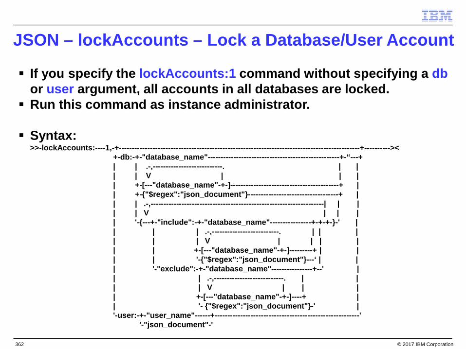
JSON – lockAccounts – Lock a Database/User Account
If you specify the lockAccounts:1 command without specifying a dbor user argument, all accounts in all databases are locked.
Run this command as instance administrator.
Syntax: >>-lockAccounts:----1,-+---------------------------------------------------------------------------------------------+---------->< +-db:-+-"database_name"---------------------------------------------------+-“---+ | | .-,---------------------------. | | | | V | | | | +-[---"database_name"-+-]------------------------------------------+ | | +-{"$regex":"json_document"}-----------------------------------+ | | | .-,-------------------------------------------------------------------| | | | | V | | | | '-{---+-"include":-+-"database_name"----------------+-+-+-}-' | | | | .-,--------------------------. | | | | | | V | | | | | | +-[---"database_name"-+-]---------+ | | | | '-{"$regex":"json_document"}---‘ | | | '-"exclude":-+-"database_name"----------------+--' | | | .-,---------------------------. | | | | V | | | | +-[---"database_name"-+-]----+ | | '- {"$regex":"json_document"}-' | '-user:-+-"user_name"------+--------------------------------------------------------' '-"json_document"-'
© 2017 IBM Corporation362

JSON – lockAccounts – Lock a Database/User Account
lockAccounts:1– Required parameter locks a database or user account.
db– Optional parameter specifies the database name of an account to lock. – For example, to lock all accounts in database that is named foo:
– db.runCommand({lockAccounts:1,db:"foo"})
exclude– Optional parameter specifies the databases to exclude. – For example, to lock all accounts on the system except those in the databases
named alpha and beta:
– db.runCommand({lockAccounts:1,db:{"exclude":["alpha","beta"]})
© 2017 IBM Corporation363

JSON – lockAccounts – Lock a Database/User Account
include– Optional parameter specifies the databases to include. – To lock all accounts in the databases named delta and gamma:
– db.runCommand({lockAccounts:1,db:{"include":["delta","gamma"]})
$regex– Optional evaluation query operator selects values from a specified JSON
document. – To lock accounts for databases that begin with the character a. and end in e:
db.runCommand({lockAccounts:1,db:{"$regex":"a.*e"})
user– Optional parameter specifies the user accounts to lock. – For example, to lock the account of all users that are not named alice:
– db.runCommand({lockAccounts:1,user:{$ne:"alice"}});© 2017 IBM Corporation364

JSON – unlockAccounts – Unlock a Database/User Account If you specify the unlockAccounts:1 without specifying a db or user
argument, all accounts in all databases are unlocked. Run this command as instance administrator.
>>-unlockAccounts:------1,-+-------------------------------------------------------------------------------------+----->< +-db:-+-"database_name"----------------------------------------------+-"-+ | | .-,---------------------------. | | | | V | | | | +-[---"database_name"-+-]-------------------------------------+ | | +-{"$regex":"json_document"}------------------------------+ | | | .-,-----------------------------------------------------------------. | | | | V | | | | '-{---+-"include":-+-"database_name"------------+-+-+-}-' | | | | .-,---------------------------. | | | | | | V | | | | | | +-[---"database_name"-+-]----- -+ | | | | '-{"$regex":"json_document"}----' | | | '-"exclude":-+-"database_name"-----------+-' | | | .-,--------------------------. | | | | V | | | | +-[---"database_name"-+-]---+ | | '-{"$regex":"json_document"}-' | '-user:-+-"user_name"-----+--------------------------------------------------' '-"json_document"-'
© 2017 IBM Corporation365

JSON – unlockAccounts – Unlock a Database/User Account unlockaccounts:1
– Required parameter unlocks a database or user account.
db– Optional parameter specifies the database name of an account to unlock. – To unlock all accounts in database that is named foo:
– db.runCommand({unlockAccounts:1,db:"foo"})
exclude– Optional parameter specifies the databases to exclude. – To unlock all accounts on the system except those in the databases named
alpha and beta:
– db.runCommand({unlockAccounts:1,db:{"exclude":["alpha","beta"]})
© 2017 IBM Corporation366
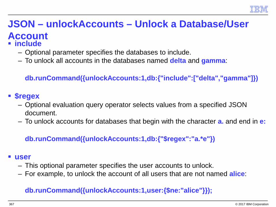
JSON – unlockAccounts – Unlock a Database/User Account include
– Optional parameter specifies the databases to include. – To unlock all accounts in the databases named delta and gamma:
– db.runCommand({unlockAccounts:1,db:{"include":["delta","gamma"]})
$regex– Optional evaluation query operator selects values from a specified JSON
document. – To unlock accounts for databases that begin with the character a. and end in e:
– db.runCommand({unlockAccounts:1,db:{"$regex":"a.*e"})
user– This optional parameter specifies the user accounts to unlock. – For example, to unlock the account of all users that are not named alice:
– db.runCommand({unlockAccounts:1,user:{$ne:"alice"}});
© 2017 IBM Corporation367

Manipulation of JSON & BSON Data Types with SQL
JSON and BSON data types, allowed in local and distributed queries, are Informix built-in data types accessible and alterable with SQL statements.
By calling BSON value functions within SQL statements it is possible to retrieve specific key values from JSON or BSON data columns.
It is possible to define indexes on key values within a JSON or BSON column.
© 2017 IBM Corporation368

High Availability for MongoDB and REST Clients
MongoDB and REST clients can be provided High Availability functionality via running a wire listener on each server in an Informix high-availability cluster
Provide high availability between the wire listener and the Informix database server:– Connect the wire listener to the database server thru the Connection Manager – Specify an sqlhosts file via the url parameter in the wire listener properties file
© 2017 IBM Corporation369

Wire Listener Configuration Enhancements
These new or updated parameters can be set in the wire listener properties file:– url parameter can include JDBC environment variables – listener.hostName parameter can specify the listener host name to control the
network adapter or interface to which the wire listener connects– collection.informix.options parameter specifies table options to automatically
add shadow columns or enable auditing during JSON collection creation– command.listDatabases.sizeStrategy parameter can specify a strategy for
computing the database size when listDatabases is executed– fragment.count parameter can specify the number of fragments to create for a
collection– jdbc.afterNewConnectionCreation parameter can specify SQL statements,
such as SET ENVIRONMENT, to run after connecting to the database server
© 2017 IBM Corporation370

Wire Listener Query Support
The wire listener now supports these types of queries:– Join queries on:
• JSON data • Relational data• Both JSON and relational data
– Array queries on JSON data with the $elemMatch query operator:• Ratings, for example, must be an arrayed column in the inventory collection
•db.inventory.find( { ratings: { $elemMatch: { $gt: 25, $lt: 90 } } } )– $first and $last group operators
© 2017 IBM Corporation371

Wire Listener Query Support (1)
Join query support is an important part of the hybrid SQL/NoSQL value proposition of Informix.
The JSON listener now supports the following running joins by querying against a new pseudo system.join table: – Collection-to-collection – Relational-to-relational – Collection-to-relational
Join queries are done by running a “find” query against the new pseudo system table called system.join.
For, example, in the Mongo shell, you’d run a query like this:
> db.system.join.find( { join query document } )
© 2017 IBM Corporation372

Wire Listener Query Support (2)
Join Query Document:
{ $collections : { “tabName1” : { join_table_specification }, “tabName2” : { join_table_specification }, … }, “$condition” : { join_condition_specification } }
Required: – $collections and $condition fields to run a find query against system.join– The $collections field must map to a document that includes two or more
collections or relational tables to be joined – The $condition specifies how to join the collections/tables. – No other query operators are supported in the top level of the join query
document (over)
© 2017 IBM Corporation373

Wire Listener Query Support (3)
The join_table_specification for each collection/table must include the required $project field; can have an optional $where query document:
– {“$project” : { … }, “$where”: { … }}
• The $project field follows the same projection syntax as regular Mongo queries • The optional $where field and uses the same query syntax as regular Mongo queries
The join_condition_specification is a document of key-value pairs that define how all of the tables specified are joined together. These conditions can be specified in two ways:– A key-string value pair to map a single table’s column to another table’s column:
– “tabName1.column1”: “tabName2.column2”
– As a key-array pair to map a table’s column to multiple other table columns
– “tabName1.column1”: – [ “tabName2.column2”, “tabName3.column3”, …. ]
© 2017 IBM Corporation374

Wire Listener Query Support – Implementation Details
Join queries work:– With the sort, limit, skip, and explain options that can be set on a Mongo
cursor– With listener cursoring
Collection-to-Collection joins:– The listener will look up if there are matching typed BSON indexes on the join
fields for each collection. • If so, it will use that bson_value_* function in the join condition to take advantage of
the index.
– If the join was on customer.customer_num and orders.customers_num and there were bson_value_int indexes on both customer.customer_num and orders.customer_num, then the listener SQL join condition would be:
•bson_value_int(customer.data, “customer_num”) = •bson_value_int(orders.data, “customer_num”)
© 2017 IBM Corporation375
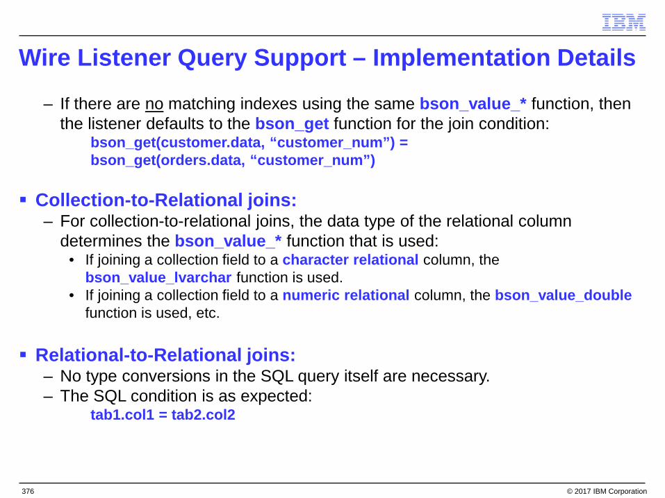
Wire Listener Query Support – Implementation Details
– If there are no matching indexes using the same bson_value_* function, then the listener defaults to the bson_get function for the join condition:
•bson_get(customer.data, “customer_num”) = •bson_get(orders.data, “customer_num”)
Collection-to-Relational joins:– For collection-to-relational joins, the data type of the relational column
determines the bson_value_* function that is used: • If joining a collection field to a character relational column, the
bson_value_lvarchar function is used. • If joining a collection field to a numeric relational column, the bson_value_double
function is used, etc.
Relational-to-Relational joins:– No type conversions in the SQL query itself are necessary. – The SQL condition is as expected:
•tab1.col1 = tab2.col2
© 2017 IBM Corporation376

Wire Listener Query Support Examples (1)
For all these examples, the tables can be collections, relational tables, or a combination of both; the syntax is the same.
Example 1: Get the customers orders that totaled more than $100. Join the customers and orders collections/tables on the customer_num field/column where the order total > 100.
{ “$collections” : { “customers” : { “$project”: { customer_num: 1, name: 1, phone: 1 } }, “orders” : { “$project”: { order_num: 1, nitems: 1, total: 1, _id: 0 }, “$where” : { total : { “$gt”: 100 } } } }, “$condition” : { “customers.customer_num” : “orders.customer_num” } }
© 2017 IBM Corporation377

Wire Listener Query Support Examples (2)
Get the IBM locations in California and Oregon. Join the companies, sites, and zipcodes collections/tables where
company name is “IBM” and state is “CA” or “OR”.
{ $collections : { “companies” : { “$project”: { name: 1, _id: 0 } “$where” : { “name” : “IBM” } }, “sites” : { “$project”: { site_name: 1, size: 1, zipcode: 1, _id:0 } }, “zipcodes” : { “$project”: { state: 1, city: 1, _id:0 } “$where” : { “state”: { “$in”, [“CA”, “OR”] } } } }, “$condition” : { “companies._id” : “sites.company_id”, “sites.zipcode” : “zipcodes.zipcode” } }
© 2017 IBM Corporation378

Wire Listener Query Support Examples (3)
Use array syntax in the condition. Get the order info, shipment info, and payment info for order number
1093.
{ $collections : { “orders” : { “$project”: { order_num: 1, nitems: 1, total: 1, _id: 0 }, “$where” : { order_num : 1093 } }, “shipments” : { “$project”: { shipment_date: 1, arrival_date: 1 } }, “payments” : { “$project”: { payment_method: 1, payment_date: 1 } } }, “$condition” : { “orders.order_num” : [ “shipments.order_num”, “payments.order_num” ] }
© 2017 IBM Corporation379

Questions
© 2017 IBM Corporation380

Agenda – Informix Warehouse Accelerator (IWA)
Load data marts faster by adding a second virtual processor for IWA.
© 2017 IBM Corporation381

Multiple VP’s for IWA Loading Performance
When initialized, IWA automatically creates a single Virtual Processor (VP) dedicated to its operations when the first IWA related activity occurs and there is no IWA VP definition in the configuration file.
This IWA VP is known internally by name as a dwavp.
The dwavp is permanently and explicitly created by the DBA at the time of initialization in the configuration file:– VPCLASS dwavp,num=1
If not explicitly added, a single dwavp virtual processor is allocated dynamically when the first IWA related activity occurs.
To add a dwavp virtual processor for the database server instance from the command line: – onmode -p +1 dwavp
© 2017 IBM Corporation399

Multiple DWAVP’s for Loading Performance
When loading multiple data marts, you can define two dwavp virtual processors to avoid administrative command delays while loading data marts.
For example, to add two dwavp virtual processors for the database server instance, in the $ONCONFIG file: – VPCLASS dwavp,num=2.
© 2017 IBM Corporation400

Devices, Platforms & Environments
Raspberry PI devices certified for V6 ARM 32 with IDS 12. IDS Developer Edition 12 for ARM V7 32 INTEL Quark (DK50) 32 bit and IDS 12 Smaller runtime embed footprint using revised onconfig settings for
devices. Mac OS 10.9 client/server support for Mac-based device developers
New 12.10.xC5 Platforms :– Mac OS X 10.8, 10.9– ARM v7– Quark– Raspberry Pi– Ubuntu 64-bit for ARM v8 (64-bit)– RHEL 7 certification for Linux x86-64 (64-bit)– PPC64
© 2017 IBM Corporation401

Miscellaneous Tivoli Work Manager 9.3 Support for Informix 12. Clear text passwords no longer passed by onstat –g ses/sql Simple REST API deployed CSDK - Improved UTF-8 support in the ODBC Driver. Advanced Enterprise Edition
– Server binaries are now stamped Advanced Enterprise with applicable license. Improved Guardium 10 support for Informix (Q3 2015).
© 2017 IBM Corporation402

Questions
© 2017 IBM Corporation403

Logo
© 2017 IBM Corporation404

Logo
© 2017 IBM Corporation405

Legal Disclaimer
• © IBM Corporation 2015. All Rights Reserved.• The information contained in this publication is provided for informational purposes only. While efforts were made to verify the completeness and accuracy of the information contained
in this publication, it is provided AS IS without warranty of any kind, express or implied. In addition, this information is based on IBM’s current product plans and strategy, which are subject to change by IBM without notice. IBM shall not be responsible for any damages arising out of the use of, or otherwise related to, this publication or any other materials. Nothing contained in this publication is intended to, nor shall have the effect of, creating any warranties or representations from IBM or its suppliers or licensors, or altering the terms and conditions of the applicable license agreement governing the use of IBM software.
• References in this presentation to IBM products, programs, or services do not imply that they will be available in all countries in which IBM operates. Product release dates and/or capabilities referenced in this presentation may change at any time at IBM’s sole discretion based on market opportunities or other factors, and are not intended to be a commitment to future product or feature availability in any way. Nothing contained in these materials is intended to, nor shall have the effect of, stating or implying that any activities undertaken by you will result in any specific sales, revenue growth or other results.
• If the text contains performance statistics or references to benchmarks, insert the following language; otherwise delete:Performance is based on measurements and projections using standard IBM benchmarks in a controlled environment. The actual throughput or performance that any user will experience will vary depending upon many factors, including considerations such as the amount of multiprogramming in the user's job stream, the I/O configuration, the storage configuration, and the workload processed. Therefore, no assurance can be given that an individual user will achieve results similar to those stated here.
• If the text includes any customer examples, please confirm we have prior written approval from such customer and insert the following language; otherwise delete:All customer examples described are presented as illustrations of how those customers have used IBM products and the results they may have achieved. Actual environmental costs and performance characteristics may vary by customer.
• Please review text for proper trademark attribution of IBM products. At first use, each product name must be the full name and include appropriate trademark symbols (e.g., IBM Lotus® Sametime® Unyte™). Subsequent references can drop “IBM” but should include the proper branding (e.g., Lotus Sametime Gateway, or WebSphere Application Server). Please refer to http://www.ibm.com/legal/copytrade.shtml for guidance on which trademarks require the ® or ™ symbol. Do not use abbreviations for IBM product names in your presentation. All product names must be used as adjectives rather than nouns. Please list all of the trademarks that you use in your presentation as follows; delete any not included in your presentation. IBM, the IBM logo, Lotus, Lotus Notes, Notes, Domino, Quickr, Sametime, WebSphere, UC2, PartnerWorld and Lotusphere are trademarks of International Business Machines Corporation in the United States, other countries, or both. Unyte is a trademark of WebDialogs, Inc., in the United States, other countries, or both.
• If you reference Adobe® in the text, please mark the first use and include the following; otherwise delete:Adobe, the Adobe logo, PostScript, and the PostScript logo are either registered trademarks or trademarks of Adobe Systems Incorporated in the United States, and/or other countries.
• If you reference Java™ in the text, please mark the first use and include the following; otherwise delete:Java and all Java-based trademarks and logos are trademarks or registered trademarks of Oracle and/or its affiliates.
• If you reference Microsoft® and/or Windows® in the text, please mark the first use and include the following, as applicable; otherwise delete:Microsoft and Windows are trademarks of Microsoft Corporation in the United States, other countries, or both.
• If you reference Intel® and/or any of the following Intel products in the text, please mark the first use and include those that you use as follows; otherwise delete:Intel, Intel Centrino, Celeron, Intel Xeon, Intel SpeedStep, Itanium, and Pentium are trademarks or registered trademarks of Intel Corporation or its subsidiaries in the United States and other countries.
• If you reference UNIX® in the text, please mark the first use and include the following; otherwise delete:UNIX is a registered trademark of The Open Group in the United States and other countries.
• If you reference Linux® in your presentation, please mark the first use and include the following; otherwise delete:Linux is a registered trademark of Linus Torvalds in the United States, other countries, or both. Other company, product, or service names may be trademarks or service marks of others.
• If the text/graphics include screenshots, no actual IBM employee names may be used (even your own), if your screenshots include fictitious company names (e.g., Renovations, Zeta Bank, Acme) please update and insert the following; otherwise delete: All references to [insert fictitious company name] refer to a fictitious company and are used for illustration purposes only.
© 2017 IBM Corporation406

© 2017 IBM Corporation407

Appendix A – Spatiotemporal Functions
© 2017 IBM Corporation

Spatiotemporal Functions – STS_Init() (1)
The STS_Init () function creates internal tables and starts a Scheduler task that builds the initial spatiotemporal index, and then periodically indexes new spatiotemporal data.
Syntax
STS_Init(ts_tabname VARCHAR(128)) returns INTEGER
STS_Init(ts_tabname VARCHAR(128) task_frequency INTERVAL DAY TO SECOND default "0 01:00:00", task_starttime DATETIME HOUR TO SECOND default NULL, ts_default_starttime DATETIME YEAR TO SECOND default "1970-01-01
00:00:00", ts_interval_to_process INTERVAL DAY TO SECOND default "0 01:00:00", ts_interval_to_avoid INTERVAL DAY TO SECOND default "1 00:00:00" ) returns INTEGER
© 2017 IBM Corporation409

Spatiotemporal Functions – STS_Init() (2)
ts_tabname – The name of the time series table.
task_frequency (optional) – How frequently to index new data. – Default is every hour.
task_starttime (Optional)– The first time to start the task. – Default is NULL, which means to start the task when the STS_Init function is run.
ts_default_starttime (Optional)– The first time stamp in the time series from which to index. – Default is 1970-01-01 00:00:00.
ts_interval_to_process (Optional)– The time interval in the time series to process each time that the task is run. – Default is one hour. – Set to a value that takes less time to index than the task_frequency parameter.
ts_interval_to_avoid (Optional)– The indexing lag time. – The time interval in the time series before the current time to avoid indexing.– Default is one day.
© 2017 IBM Corporation410

Spatiotemporal Functions – STS_Init() (3)
Run STS_Init () to start the indexing process by creating internal spatiotemporal search tables and starting a Scheduler task for the specified table. – The Scheduler task, which has a prefix of autosts, starts at the time specified
by the task_starttime parameter, indexes the initial set of data, and periodically indexes new data.
– The task prints messages in the database server message log when indexing starts and completes.
– If spatiotemporal search indexing is already running for the specified table, run the STS_Init() to change the Scheduler task properties.
The first run of the task processes the data in the time interval that is defined by the value of the ts_default_starttime parameter:– ts_default_starttime = current_time - ts_interval_to_avoid
© 2017 IBM Corporation411

Spatiotemporal Functions – STS_Init() (4)
The end time of the processing interval is saved in the internal lasttimetable. Subsequent runs of the task start based on the value of the task_frequency parameter and index the data between the last end time that is saved in the lasttime table and the earlier of the following times:– The last end time plus the value of the ts_interval_to_process parameter– The current time minus the value of the ts_interval_to_avoid parameter
Any data that you insert with timepoints that are earlier than the last end time that is saved in the lasttime table are not indexed.
If you run the task the first time on an empty time series, the recorded last end time is the current time minus the value of the parameter ts_interval_to_avoid. – Any data that you insert with earlier timepoints are not indexed.
Returns 0 or 1 - an integer that indicates the status of the function:– 0 = The Scheduler task for spatiotemporal search indexing started.– 1 = An error occurred.
© 2017 IBM Corporation412
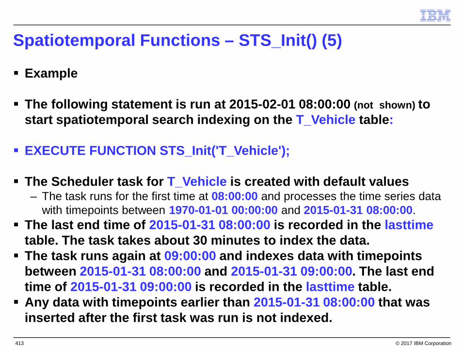
Spatiotemporal Functions – STS_Init() (5)
Example
The following statement is run at 2015-02-01 08:00:00 (not shown) to start spatiotemporal search indexing on the T_Vehicle table:
EXECUTE FUNCTION STS_Init('T_Vehicle');
The Scheduler task for T_Vehicle is created with default values – The task runs for the first time at 08:00:00 and processes the time series data
with timepoints between 1970-01-01 00:00:00 and 2015-01-31 08:00:00. The last end time of 2015-01-31 08:00:00 is recorded in the lasttime
table. The task takes about 30 minutes to index the data. The task runs again at 09:00:00 and indexes data with timepoints
between 2015-01-31 08:00:00 and 2015-01-31 09:00:00. The last end time of 2015-01-31 09:00:00 is recorded in the lasttime table.
Any data with timepoints earlier than 2015-01-31 08:00:00 that was inserted after the first task was run is not indexed.
© 2017 IBM Corporation413

STS_Cleanup() (1)
Stop spatiotemporal search indexing and drop internal tables. Syntax
– STS_Cleanup(ts_tabname VARCHAR(128)) returns INTEGER– STS_Cleanup() returns INTEGER
– ts_tabname (Optional) - The name of the time series table.
Usage– Run with the ts_tabname parameter when you want to stop spatiotemporal
indexing and drop the existing spatiotemporal search tables for the specified time series table:
•When the spatiotemporal search tables becomes large, you can drop them and then restart spatiotemporal search indexing with a more recent start time.
– Run without a parameter to stop spatiotemporal indexing and drop the existing spatiotemporal search tables for the current database.
Returns– An integer that indicates the status of the function:– 0 = Spatiotemporal search indexing was removed.– 1 = An error occurred.
© 2017 IBM Corporation414

STS_Cleanup() (2)
Example: – Stop indexing and drop index tables for a table
The following statement stops spatiotemporal search indexing and deletes the internal tables for the time series table T_Vehicle:
EXECUTE FUNCTION STS_Cleanup('T_Vehicle');
Example: – Stop indexing and drop index tables for a database
The following statement stops spatiotemporal search indexing and deletes the internal tables for the current database:
EXECUTE FUNCTION STS_Cleanup();
© 2017 IBM Corporation415

STS_GetPosition() (1)
Find the position of an object at a specific time:
Syntax
STS_GetPosition(ts TimeSeries, tstamp DATETIME YEAR TO FRACTION(5)) returns LVARCHAR
ts The time series. tstamp The time stamp to query.
© 2017 IBM Corporation416

STS_GetPosition() (2)
To identify which object to track is defined in the WHERE clause of the query.
Returns– An LVARCHAR string that represents the position of the object. – The string includes the spatial reference ID (SRID 4326) and a point that consists
of a longitude value and a latitude value.– NULL, if nothing found.
Example– The following query returns the position of the vehicle 1 at 2014-02-02 13:34:06:
SELECT STS_GetPosition(ts_track, '2014-02-02 13:34:06') FROM T_Vehicle WHERE modid='1';
(expression) 4326 point(116.400610 39.906050)
© 2017 IBM Corporation417

STS_GetLastPosition() (1)
Find the most recent position of any object in the time series:
Syntax
STS_GetPosition(ts TimeSeries, tstamp DATETIME YEAR TO FRACTION(5)) returns LVARCHAR
ts The time series. tstamp The time stamp to query.
© 2017 IBM Corporation418

STS_GetLastPosition() (2)
Run STS_GetPosition() to find where a moving object was at a specific time.
To identify which object to track is in the WHERE clause of the query.
Returns:– An LVARCHAR string that represents the position of the object. – The string includes the spatial reference ID (4326) and a point that consists of a
longitude value and a latitude value.– Or NULL, if nothing found.
Example:– The following query returns the position of the vehicle 2 at 2014-02-02 18:38:06:– SELECT STS_GetPosition(ts_track, '2014-02-02 18:38:06') – FROM T_Vehicle – WHERE modid=‘2';
– (expression) 4326 point(116.400610 39.906050)
© 2017 IBM Corporation419

STS_GetFirstTimeByPoint() (1) Find the first time in a time range when an object is near a position Syntax STS_GetFirstTimeByPoint(ts_tabname LVARCHAR, obj_id LVARCHAR, ts TimeSeries, starttime DATETIME YEAR TO FRACTION(5), endtime DATETIME YEAR TO FRACTION(5), geometry LVARCHAR, max_distance REAL) returns DATETIME
STS_GetFirstTimeByPoint(ts_tabname LVARCHAR, obj_id LVARCHAR, ts TimeSeries, starttime DATETIME YEAR TO FRACTION(5), endtime DATETIME YEAR TO FRACTION(5), geometry LVARCHAR, max_distance REAL, uom LVARCHAR) returns DATETIME
© 2017 IBM Corporation420

STS_GetFirstTimeByPoint() (2)
Syntax (cont’d)
ts_tabname– The name of the time series table.
obj_id– The ID of the object. – Must be a value from the primary key column of the time series table. – Can be the name of the column that stores the object IDs if the WHERE clause
specifies a specific object ID. ts
– The name of the TimeSeries data type. starttime
– The start of the time range. – Can be NULL.
endtime– The end of the time range. – Can be NULL.
© 2017 IBM Corporation421

STS_GetFirstTimeByPoint() (3)
Syntax (cont’d)
geometry– The geometry at the center of the region of interest. – Can be an ST_Point, ST_MultiPoint, ST_LineString, ST_MultiLineString,
ST_Polygon, or ST_MultiPolygon. – Must use the SRID 4326.
max_distance– The distance from the geometry that defines the border of the region of interest.– The unit of measure is specified by the uom parameter.
uom (Optional)
– The unit of measure for the max_distance parameter. – Default is meters. – Must be the name of a linear unit of measure from the unit_name column of
the st_units_of_measure table.
© 2017 IBM Corporation422

STS_GetFirstTimeByPoint() (4)
Usage
Run STS_GetFirstTimeByPoint () to find when an object first passed within the specified distance of the specified position during the specified time range. – If you do not specify a time range, the function returns the first time that an
object passed close enough to the position. – If the object was too far away from the position during the time range, the
STS_GetFirstTimeByPoint function returns NULL.
Returns– A time stamp– NULL if the trajectory of the object during the time range was always farther
than the maximum distance from the position.
Example: Find the first time that the vehicle ever passed the position
© 2017 IBM Corporation423

STS_GetFirstTimeByPoint() (5)
The following query returns the first time ever that vehicle 1 passed within 100 meters of the point (116.401 39.911):
SELECT STS_GetFirstTimeByPoint('T_Vehicle', modid, ts_track, null, null, '4326 point(116.401 39.911)', 100) FROM T_Vehicle WHERE modid = '1';
(expression)
2014-02-02 13:37:15.00000
1 row(s) retrieved.
Example: Find the first time that the vehicle passed the position in a time range
© 2017 IBM Corporation424

STS_GetFirstTimeByPoint() (6)
The following query returns the first time that vehicle 1 passed within 100 meters of the point (116.401 39.911) between 2014-02-02 13:39:00 and 2014-02-02 16:30:00:
SELECT STS_GetFirstTimeByPoint ('T_Vehicle', modid, ts_track, '2014-02-02 13:39:00', '2014-02-02 16:30:00', '4326 point(116.40100 39.91100)', 100) FROM T_Vehicle WHERE modid='1';
(expression)
2014-02-02 13:40:55.00000
1 row(s) retrieved.
© 2017 IBM Corporation425

STS_GetNearestObject() (1)
Find the nearest object to a point at a specific time. Syntax
STS_GetNearestObject(ts_tabname LVARCHAR, ts_colname LVARCHAR, timestamp DATETIME YEAR TO FRACTION(5), geometry LVARCHAR, max_distance REAL) returns LVARCHAR
STS_GetNearestObject(ts_tabname LVARCHAR, ts_colname LVARCHAR, timestamp DATETIME YEAR TO FRACTION(5), geometry LVARCHAR, max_distance REAL, uom LVARCHAR) returns LVARCHAR
© 2017 IBM Corporation426

TS_GetNearestObject() (2)
ts_tabname– The name of the time series table.
ts_colname– The name of the TimeSeries column.
timestamp– The time point to query.
geometry– The geometry at the center of the region of interest. – Can be an ST_Point, ST_MultiPoint, ST_LineString, ST_MultiLineString,
ST_Polygon, or ST_MultiPolygon. – Must use the SRID 4326.
max_distance– The distance from the geometry that defines the border of the region of interest.– The unit of measure is specified by the uom parameter.
uom (Optional)
– The unit of measure for the max_distance parameter. – The default is meters. – Must be the name of a linear unit of measure from the unit_name column of
the st_units_of_measure table.© 2017 IBM Corporation427

TS_GetNearestObject() (3)
Usage– Run STS_GetNearestObject to find which object was closest to a location but
within a specific distance at a specific time. – If you specify that 0 meters distance from the point, STS_GetNearestObject
returns the closest object regardless of the distance.
Returns– The object ID.– Or NULL, if nothing found.
Example– The following statement returns the vehicle ID whose location was the closest
to the point (10,10), but within 1010 meters, at 2014-02-02 13:36:00:
EXECUTE FUNCTION STS_GetNearestObject('T_Vehicle', 'ts_track', '2014-02-02 13:36:00', '4326 point(116.4 39.9)', 1010);– (expression) 1
1 row(s) retrieved.© 2017 IBM Corporation428

STS_GetTrajectory() (1)
Find the exact trajectory for a time range
Syntax: STS_GetTrajectory(ts TimeSeries, starttime DATETIME YEAR TO FRACTION(5), endtime DATETIME YEAR TO FRACTION(5)) returns LVARCHAR
ts– The time series.
starttime– The start of the time range.
endtime– The end of the time range.
© 2017 IBM Corporation429

STS_GetTrajectory() (2)
Run STS_GetTrajectory to find where an object went (its path) during a time range, which is based on the data in the time series table.
The location for each time point in the range is extracted from the time series table and converted into one or more linestrings.
Identify which object to track in the WHERE clause of the query.
Returns– An LVARCHAR string that represents the trajectory of the object.
•The string includes the spatial reference ID and a multilinestring that consists of multiple sets of longitude and latitude values.
– NULL, if nothing found.
Example: Get the trajectory between specific times
© 2017 IBM Corporation430

STS_GetTrajectory() (3)
Example:
The following query returns the trajectory of the vehicle 1 between 2014-02-02 13:00:00 and 2014-02-02 16:30:00:
SELECT STS_GetTrajectory (ts_track, '2014-02-02 13:00:00', '2014-02-02 16:30:00') FROM T_Vehicle WHERE modid='1';
(expression)
4326 multilinestring((116.400610 39.906050, 116.401210 39.913900, 116.401170 39.911590, 116.392450 39.906350, 116.369990 39.905940, 116.345260 39.905890))
1 row(s) retrieved.© 2017 IBM Corporation431

STS_GetTrajectory() (4) Example: Get the trajectory from a specific time until the current time
The following query returns the trajectory of the vehicle 1 between 2014-02-02 13:00:00 and the current time:
SELECT STS_GetTrajectory (ts_track, '2014-02-02 13:00:00', current) FROM T_Vehicle WHERE modid='1';
(expression) 4326 multilinestring((116.400610 39.906050, 116.401210 39.913900, 116.401170 39.911590, 116.392450 39.906350, 116.369990 39.905940, 116.345260 39.905890),(116.420000 40.100000, 116.401000 39.907000, 116.402000 39.908000, 116.402010 39.908010))
1 row(s) retrieved.© 2017 IBM Corporation432

STS_GetCompactTrajectory() (1)
STS_GetCompactTrajectory returns the compressed trajectory of a specified object for the specified time range.
Syntax
STS_GetCompactTrajectory(ts_tabname LVARCHAR, obj_id LVARCHAR, ts TimeSeries, starttime DATETIME YEAR TO FRACTION(5), endtime DATETIME YEAR TO FRACTION(5)) returns LVARCHAR
© 2017 IBM Corporation433

STS_GetCompactTrajectory() (2)
ts_tabname– The name of the time series table.
obj_id– The ID of the object. – Must be a value from the primary key column of the time series table. – Can be the name of the column that stores the object IDs if the WHERE clause
specifies a specific object ID. ts
– The name of the TimeSeries column. starttime
– The start of the time range. endtime
– The end of the time range.
© 2017 IBM Corporation434

STS_GetCompactTrajectory() (3)
Run STS_GetCompactTrajectory to find where an object went during a time range, based on the compressed spatiotemporal search data. The trajectory information is retrieved from the subtack table and returned as one or more linestrings.
Returns– An LVARCHAR string that represents the trajectory of the object.
•The string includes the spatial reference ID and an ST_MultiLinestring.– NULL, if nothing found.
© 2017 IBM Corporation435

STS_GetCompactTrajectory() (4)
Example
The following query returns the trajectory of the vehicle 1 between 2014-02-02 13:00:00 and 2014-02-02 16:30:00:
SELECT STS_GetCompactTrajectory('T_Vehicle', modid, 'ts_track', '2014-02-02 13:00:00', '2014-02-02 16:30:00') FROM T_Vehicle WHERE modid='1';
(expression)
4326 multilinestring((116.40061 39.90605, 116.40121 39.9139, 116.40117 39.91159, 116.39245 39.90635, 116.36999 39.90594, 116.345261 39.905891, 116.345261 39.905891))
1 row(s) retrieved.© 2017 IBM Corporation436

STS_GetIntersectSet() (1)
The set of objects whose trajectories intersected a region during the time range.
Syntax STS_GetIntersectSet(ts_tabname LVARCHAR, ts_colname LVARCHAR, starttime DATETIME YEAR TO FRACTION(5), endtime DATETIME YEAR TO FRACTION(5), geometry LVARCHAR, max_distance REAL) returns Set(LVARCHAR)
STS_GetIntersectSet(ts_tabname LVARCHAR, ts_colname LVARCHAR, starttime DATETIME YEAR TO FRACTION(5), endtime DATETIME YEAR TO FRACTION(5), geometry LVARCHAR, max_distance REAL, uom LVARCHAR) returns Set(LVARCHAR)
© 2017 IBM Corporation437

STS_GetIntersectSet() (2)
Syntax (cont’d)
ts_tabname– The name of the time series table.
ts_column– The name of the TimeSeries column.
starttime– The start of the time range.
endtime– The end of the time range.
geometry– The geometry at the center of the region of interest. – Can be an ST_Point, ST_MultiPoint, ST_LineString, ST_MultiLineString,
ST_Polygon, or ST_MultiPolygon. – Must use the SRID 4326.
max_distance– The distance from the geometry that defines the border of the region of interest.– The unit of measure is specified by the uom parameter.
© 2017 IBM Corporation438

STS_GetIntersectSet() (3)
Syntax (cont’d)
uom (Optional)
– The unit of measure for the max_distance parameter. – The default is meters. – Must be the name of a linear unit of measure from the unit_name column of
the st_units_of_measure table.
Usage
Run STS_GetIntersectSet to find which objects intersected a region during a time range.
Returns– A set of object IDs.– NULL, if nothing found.
© 2017 IBM Corporation439

STS_GetIntersectSet() (4)
Example
The following statement returns the vehicles IDs that intersected the region within 1000 meters of the point (116.4, 39.91) during the time between 2014-02-02 13:36:00 and 2014-02-02 13:54:00:
EXECUTE FUNCTION STS_GetIntersectSet ('T_Vehicle', 'ts_track', '2014-02-02 13:36:00', '2014-02-02 13:54:00',
'4326 point(116.4 39.91)', 1000);
(expression) SET{'1','2'}
1 row(s) retrieved.
The query returned the IDs 1 and 2.
© 2017 IBM Corporation440

STS_GetLocWithinSet() (1)
The set of objects that were within a region at a specific time:
Syntax: STS_GetLocWithinSet(ts_tabname LVARCHAR, ts_colname LVARCHAR, timestamp DATETIME YEAR TO FRACTION(5), geometry LVARCHAR, max_distance REAL) returns Set(LVARCHAR)
STS_GetLocWithinSet(ts_tabname LVARCHAR, ts_colname LVARCHAR, timestamp DATETIME YEAR TO FRACTION(5), geometry LVARCHAR, max_distance REAL, uom LVARCHAR) returns Set(LVARCHAR)
© 2017 IBM Corporation441

STS_GetLocWithinSet() (2)
ts_tabname– The name of the time series table.
ts_colname– The name of the TimeSeries column.
timestamp– The time point to query.
geometry– The geometry at the center of the region of interest. – Can be an ST_Point, ST_MultiPoint, ST_LineString, ST_MultiLineString,
ST_Polygon, or ST_MultiPolygon. – Must use the SRID 4326.
max_distance– The distance from the geometry that defines the border of the region of interest.
The unit of measure is specified by the uom parameter. uom (optional)
– The unit of measure for the max_distance parameter. – The default is meters. – Must be the name of a linear unit of measure from the unit_name column of
the st_units_of_measure table.© 2017 IBM Corporation442

STS_GetLocWithinSet() (3)
Run STS_GetLocWithinSet () to find which objects were in a region at a specific time.
Returns– A set of object IDs.– NULL, if nothing found.
Example
The following statement returns the IDs of vehicles that were within 1000 meters of the point (116.4, 39.91) at 2014-02-02 13:36:00:
EXECUTE FUNCTION STS_GetLocWithinSet('T_Vehicle', 'ts_track', '2014-02-02 13:36:00', '4326 point(116.4 39.91)', 1000);
(expression) SET{'1','2'}
The query returns the IDs 1 and 2.© 2017 IBM Corporation443

STS_TrajectoryDistance() (1)
The shortest distance between a point and the trajectory of an object during a time range.
Syntax STS_TrajectoryDistance(ts_tabname LVARCHAR, obj_id LVARCHAR, ts_colname LVARCHAR, starttime DATETIME YEAR TO FRACTION(5), endtime DATETIME YEAR TO FRACTION(5), geometry LVARCHAR) returns FLOAT STS_TrajectoryDistance(ts_tabname LVARCHAR, obj_id LVARCHAR, ts_colname LVARCHAR, starttime DATETIME YEAR TO FRACTION(5), endtime DATETIME YEAR TO FRACTION(5), geometry LVARCHAR, uom LVARCHAR) returns FLOAT
© 2017 IBM Corporation444
STS_TrajectoryDistance() (2)
ts_tabname– The name of the time series table.
obj_id– The ID of the object. – Must be a value from the primary key column of the time series table. – Can be the name of the column that stores the object IDs if the WHERE clause
specifies a specific object ID. ts_colname
– The name of the TimeSeries column. starttime
– The start of the time range. – Can be NULL.
endtime– The end of the time range. – Can be NULL.
© 2017 IBM Corporation445

STS_TrajectoryDistance() (3)
Syntax (cont’d)
geometry– The geometry at the center of the region of interest. – Can be an ST_Point, ST_MultiPoint, ST_LineString, ST_MultiLineString,
ST_Polygon, or ST_MultiPolygon. – Must use the SRID 4326.
uom (optional)
– The unit of measure for the return value. – The default is meters.– Must be the name of a linear unit of measure from the unit_name column of
the st_units_of_measure table.
Run STS_TrajectoryDistance () to find how close and object came to a specific point during a time range.
© 2017 IBM Corporation446

STS_TrajectoryDistance() (4)
Returns– A FLOAT value that represents the distance in the specified unit of measure.– NULL, if nothing found.
Example The following query returns the shortest distance in meters between
the trajectory of vehicle 1 and the point (116.4. 39.9) between 2014-02-02 13:35:00 and 2014-02-02 13:54:00:
SELECT STS_TrajectoryDistance ('T_Vehicle', modid, 'ts_track', '2014-02-02 13:35:00', '2014-02-02 13:54:00', '4326 point(116.4 39.9)')::decimal(10,2) FROM T_Vehicle WHERE modid='1';
(expression) 830.36
1 row(s) retrieved.© 2017 IBM Corporation447

STS_TrajectoryWithin() (1)
Indicates whether the trajectory of a specified object stayed within the specified region during the specified time range.
Syntax STS_TrajectoryWithin(ts_tabname LVARCHAR, obj_id LVARCHAR, ts_colname LVARCHAR, starttime DATETIME YEAR TO FRACTION(5), endtime DATETIME YEAR TO FRACTION(5), geometry LVARCHAR, max_distance REAL) returns Boolean STS_TrajectoryWithin(ts_tabname LVARCHAR, obj_id LVARCHAR, ts_colname LVARCHAR, starttime DATETIME YEAR TO FRACTION(5), endtime DATETIME YEAR TO FRACTION(5), geometry LVARCHAR, max_distance REAL, uom LVARCHAR) returns Boolean © 2017 IBM Corporation448

STS_TrajectoryWithin() (2)
ts_tabname– The name of the time series table.
obj_id– The ID of the object. – Must be a value from the primary key column of the time series table. – Can be the name of the column that stores the object IDs if the WHERE clause
specifies a specific object ID. ts_colname
– The name of the TimeSeries column. starttime
– The start of the time range. Can be NULL. endtime
– The end of the time range. Can be NULL. geometry
– The geometry at the center of the region of interest. – Can be an ST_Point, ST_MultiPoint, ST_LineString, ST_MultiLineString,
ST_Polygon, or ST_MultiPolygon. – Must use the SRID 4326.
© 2017 IBM Corporation449

STS_TrajectoryWithin() (3)
max_distance– The distance from the geometry that defines the border of the region of interest.– The unit of measure is specified by the uom parameter.
uom (optional)
– The unit of measure for the max_distance parameter. – The default is meters. – Must be the name of a linear unit of measure from the unit_name column of
the st_units_of_measure table.
Usage
Run STS_TrajectoryWithin to find out whether an object stayed within a region during the entire time range. – STS_TrajectoryWithin returns ‘f’ if the object was in the region for only part of
the time range or if the object was never in the region during the time range.
© 2017 IBM Corporation450

STS_TrajectoryWithin() (4) Returns
– t•If the trajectory of the object was within the region during the entire time range.
– f•If the trajectory of the object was within the region for only part of the time range.•If the trajectory of the object was not within the region during the time range.
The following query returns whether vehicle 1 stayed within 1000 meters of the point (116.4, 39.91) between 2014-02-02 13:34:00 and 2014-02-02 13:54:00:
SELECT STS_TrajectoryWithin ('T_Vehicle', modid, 'ts_track', '2014-02-02 13:34:00', '2014-02-02 13:54:00', '4326 point(116.4 39.91)', 1000) FROM T_Vehicle WHERE modid='1';
(expression) f 1 row(s) retrieved. © 2017 IBM Corporation451
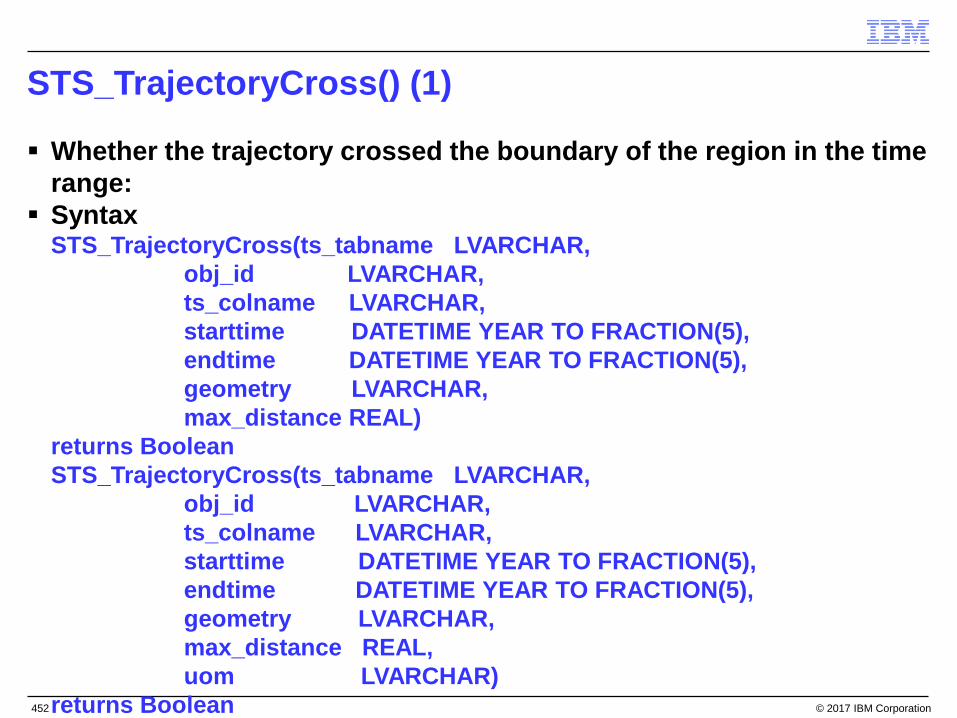
STS_TrajectoryCross() (1)
Whether the trajectory crossed the boundary of the region in the time range:
Syntax STS_TrajectoryCross(ts_tabname LVARCHAR, obj_id LVARCHAR, ts_colname LVARCHAR, starttime DATETIME YEAR TO FRACTION(5), endtime DATETIME YEAR TO FRACTION(5), geometry LVARCHAR, max_distance REAL) returns Boolean STS_TrajectoryCross(ts_tabname LVARCHAR, obj_id LVARCHAR, ts_colname LVARCHAR, starttime DATETIME YEAR TO FRACTION(5), endtime DATETIME YEAR TO FRACTION(5), geometry LVARCHAR, max_distance REAL, uom LVARCHAR) returns Boolean © 2017 IBM Corporation452

STS_TrajectoryCross() (2)
ts_tabname– The name of the time series table.
obj_id– The ID of the object. – Must be a value from the primary key column of the time series table. – Can be the name of the column that stores the object IDs if the WHERE clause
specifies a specific object ID. ts_colname
– The name of the TimeSeries column. starttime
– The start of the time range. endtime
– The end of the time range. geometry
– The geometry at the center of the region of interest. – Can be an ST_Point, ST_MultiPoint, ST_LineString, ST_MultiLineString,
ST_Polygon, or ST_MultiPolygon. – Must use the SRID 4326.
© 2017 IBM Corporation453

STS_TrajectoryCross() (3)
max_distance– The distance from the geometry that defines the border of the region of interest.– The unit of measure is specified by the uom parameter.
uom (optional)
– The unit of measure for the max_distance parameter. – The default is meters. – Must be the name of a linear unit of measure from the unit_name column of
the st_units_of_measure table.
Run STS_TrajectoryCross () to know whether an object crossed the boundary of a specific region during a time range.
STS_TrajectoryCross () – Returns t if the object crossed the boundary of the region one or more times
during the time range. – Returns f if the object remained either outside or inside of the region for the
time range (did not cross the boundary).
© 2017 IBM Corporation454

STS_TrajectoryCross() (4)
The following query returns whether vehicle 1 crossed the boundary of the region, which is specified by the point (116.4, 39.91) and the distance of 1000 meters, between 2014-02-02 13:34:00 and 2014-02-02 13:54:00:
SELECT STS_TrajectoryCross ('T_Vehicle', modid, 'ts_track', '2014-02-02 13:34:00', '2014-02-02 13:54:00', '4326 point(116.4 39.91)', 1000) FROM T_Vehicle WHERE modid = '1';
(expression)
t
1 row(s) retrieved.
© 2017 IBM Corporation455

STS_TrajectoryIntersect()(1)
Indicates whether the trajectory either crossed or remained within, the boundary of the region for the time range.
Syntax STS_TrajectoryIntersect(ts_tabname LVARCHAR, obj_id LVARCHAR, ts_colname LVARCHAR, starttime DATETIME YEAR TO FRACTION(5), endtime DATETIME YEAR TO FRACTION(5), geometry LVARCHAR, max_distance REAL) returns Boolean STS_TrajectoryIntersect(ts_tabname LVARCHAR, obj_id LVARCHAR, ts_colname LVARCHAR, starttime DATETIME YEAR TO FRACTION(5), endtime DATETIME YEAR TO FRACTION(5), geometry LVARCHAR, max_distance REAL, uom LVARCHAR) returns Boolean © 2017 IBM Corporation456

STS_TrajectoryIntersect()(2)
ts_tabname– The name of the time series table.
obj_id– The ID of the object. – Must be a value from the primary key column of the time series table. – Can be the name of the column that stores the object IDs if the WHERE clause
specifies a specific object ID. ts_colname
– The name of the TimeSeries column. starttime
– The start of the time range. endtime
– The end of the time range. geometry
– The geometry at the center of the region of interest. – Can be an ST_Point, ST_MultiPoint, ST_LineString, ST_MultiLineString,
ST_Polygon, or ST_MultiPolygon. – Must use the SRID 4326.
© 2017 IBM Corporation457

STS_TrajectoryIntersect()(3)
max_distance– The distance from the geometry that defines the border of the region of interest.– The unit of measure is specified by the uom parameter.
uom (optional)
– The unit of measure for the max_distance parameter. – The default is meters. – Must be the name of a linear unit of measure from the unit_name column of
the st_units_of_measure table.
Run STS_TrajectoryIntersect () to find out whether the specified object went through the specified region during the specified time range.– Intersection means either crossed the boundary of the region or remained
within the boundary of the region.
© 2017 IBM Corporation458

STS_TrajectoryIntersect()(4)
Returns– t
•If the trajectory of the object crossed the boundary of the region during the time range.•If the trajectory of the object remained within the region during the time range.
– f•if the trajectory of the object did not intersect the region during the time range.
© 2017 IBM Corporation459

STS_TrajectoryIntersect()(5)
The following query returns whether vehicle 1 intersected the boundary of the region, which is described by the point (116.4, 39.91) and the distance of 1000 meters, between 2014-02-02 13:34:00 and 2014-02-02 13:54:00:
SELECT STS_TrajectoryIntersect ('T_Vehicle', modid, 'ts_track', '2014-02-02 13:34:00', '2014-02-02 13:54:00', '4326 point(116.4 39.91)', 1000) FROM T_Vehicle WHERE modid = '1';
(expression)
t
1 row(s) retrieved.
© 2017 IBM Corporation460

STS_Release()
The STS_Release function returns the internal version number and build date for the spatiotemporal search extension.
Syntax
STS_Release() Returns LVARCHAR;
Returns– A string with the version number and build date.
The following statement returns the version number and build date:
EXECUTE FUNCTION STS_Release;
© 2017 IBM Corporation461

STS_Set_Trace() procedure (1)
STS_Set_Trace enables tracing and sets the tracing file. Syntax
STS_Set_Trace(trace_params LVARCHAR, trace_file LVARCHAR);
trace_params– The tracing parameters in the following format:
•tracing_type tracing_level:•tracing_type
– STSQuery: Set tracing on spatiotemporal queries.– STSBuild: Set tracing on spatiotemporal indexing.
•tracing_level• 0 = Turn off tracing.
>1 = Any integer greater than 1 = Turn on tracing. trace_file
– The full path and name of the tracing file.
© 2017 IBM Corporation462
STS_Set_Trace() procedure (2)
Run STS_Set_Trace with the STSQuery value to enable tracing if you want to view the entry points of spatiotemporal query functions.
Run STS_Set_Trace with the STSBuild value to enable tracing if you want to view the entry points of spatiotemporal indexing functions. – You must specify the full path and name of the tracing file.
© 2017 IBM Corporation463

STS_Set_Trace() procedure (3)
Set query tracing
The following statement starts tracing on spatiotemporal queries and sets the tracing file name and path:
EXECUTE PROCEDURE STS_Set_Trace('STSQuery 2', '/tms/sts_query.log');
Stop query tracing
The following statement stops tracing on spatiotemporal queries:
EXECUTE PROCEDURE STS_Set_Trace('STSQuery 0', '/tms/sts_query.log');
© 2017 IBM Corporation464

Appendix B – Spatiotemporal Catalog Tables
© 2017 IBM Corporation

STS_DefaultParameters Table
Contains the default parameters document for the database and the table is empty until you run the STS_SetDefaultParameters function. If you omit the parameters document from the STS_SubtrackCreatefunction, the values in this table are used.
The STS_DefaultParametersTable table contains a parameterscolumn, which is of type BSON, and only one row, which contains the default parameters document.
You can update the default parameters document with the STS_SetDefaultParameters function. The existing default parameters document is replaced.
© 2017 IBM Corporation466

STS_InstanceTable
The table contains the association between a time series instance and a subtrack definition.
Every time series that has subtrack records in a subtrack table has a row in the STS_InstanceTable table.
The following table lists the columns of the STS_InstanceTable table:
The time series instance ID is listed in the TSInstanceTable table.
Column Data Type Descriptioninstance_id BIGINT Time Series instance ID. The primary keysubtrack_id INTEGER Unique ID of the subtrack table
© 2017 IBM Corporation467

STS_SubtrackTableColumn name Data type Descriptionsubtrack_id SERIAL The unique ID of the subtrack table.
subtrack_name VARCHAR(128) The name of the subtrack table. The primary key.
base_table_name VARCHAR(128) The name of the time series table.
ts_column_name VARCHAR(128) The time series column name in the time series table.
flags INTEGER Specifies whether a Scheduler task indexes new data:1 = A Scheduler task is running. 2 = No Scheduler task.
parameters BSON A BSON document that contains parameters to build the subtrack.
ts_data_first_timestamp DATETIME YEAR TO SECOND
First time stamp in the time series to index with the Scheduler task.
ts_data_lag_to_current INTERVAL DAY TO SECOND
Time interval before current time to avoid indexing with the Scheduler task.
task_nschsessions INTEGER Number of Scheduler sessions to start to update the index in parallel.
task_frequency INTERVAL DAY TO SECOND
How frequently to index new data with the Scheduler task.
task_start_time DATETIME HOUR TO SECOND
First time to start the Schedule task.
task_data_interval_to_process INTERVAL DAY TO SECOND
Time interval in the time series to process each time that the Scheduler task is run. © 2017 IBM Corporation468

STS_SubtrackTable
The STS_SubtrackTable table contains the subtrack definitions.
When you run the STS_SubtrackCreate function, a row is added to the STS_SubtrackTable table.
© 2017 IBM Corporation469

Subtrack table
Column name Data type Descriptioninstance_id BIGINT The time series instance ID.
begin_time DATETIME YEAR TO FRACTION(5)
The start time of the entry.
end_time DATETIME YEAR TO FRACTION(5)
The end time of the entry.
state SMALLINT The type of entry:0 = Moving. The geometry column contains a trajectory.1 = Stationary. The geometry column contains a location.2 = No signal. The object had no signal for the time period between the start time and the end time, and the object is in the same location.3 = Interrupted signal. The object had no signal for the time period between the start time and the end time, and the object is in a different location.
geometry ST_Geometry Depends on the value of the state column:0 = An ST_LineString or ST_MultiLineString that represents the trajectory of the object.1 = An ST_Point that represents the location of the object.2 or 3 = NULL
Contains spatiotemporal data for the associated time series column. You specify the name of the subtrack table when you run the
STS_SubtrackCreate function.
© 2017 IBM Corporation470

Appendix C – Regex Character Names.
© 2017 IBM Corporation

Regex Character Names (1 of 4)
Name Code Name Code
soh 01 = Start of heading newline 0A (LF) = Line feed
stx 02 = Start of text vt 0B = Vertical tab
etx 03 = End of text vertical-tab 0B (VT) = Vertical tab
eot 04 = End of transmission ff 0C (FF) = Form feed
enq 05 = Enquiry form-feed 0C (FF) = Form feed
ack 06 = Acknowledgment cr 0D (CR) = Carriage return
bel 07 = Bell carriage-return 0D (CR) = Carriage return
alert 07 (BEL) = Bell so 0E = Shift Out/X-On
bs 08 = Backspace si 0F = Shift In/X-Off
backspace 08 = Backspace dle 10 = Data line escape
ht 09 = Horizontal tab dc1 11 = Device control 1
tab 09 (HT) = Horizontal tab dc2 12 = Device control 2
lf 0A = Line feed dc3 13 = Device control 3
© 2017 IBM Corporation472

Regex Character Names (2 of 4)
Name Code Name Code
syn 16 = Synchronous idle space ' '
etb 17 = End of transmit block exclamation-mark '!'
can 18 = Cancel quotation-mark '"'
em 19 = End of medium number-sign '#'
sub 1A = Substitute dollar-sign '$'
esc 1B = Escape percent-sign '%'
is4 1C (FS) = File separator ampersand '&'
fs 1C = File separator apostrophe '\'
is3 1D (GS) = Group separator left-parenthesis '('
gs 1D (GS) = Group separator right-parenthesis ')'
is2 1E (RS) = Record separator asterisk '*'
rs 1E (RS) = Record separator plus-sign '+'
is1 1F (US) = Unit separator comma ,
us 1F (US) = Unit separator hyphen '-'© 2017 IBM Corporation473

Regex Character Names (3 of 4)Name Code Name Code
hyphen-minus - Colon :period '.' semicolon ';'full-stop '.' less-than-sign '<'Slash / equals-sign '='solidus '/' greater-than-sign '>'Zero 0 question-mark ?one '1' commercial-at @
two '2' left-square-bracket '['
Three 3 backslash \
four 4 reverse-solidus \
Five 5 right-square-bracket ]
six '6' circumflex ^'
Seven 7 circumflex-accent ^'
Eight 8 underscore _'
Nine 9 low-line _'© 2017 IBM Corporation474

Regex Character Names (4 of 4)Name Code Name Code
grave-accent `left-brace '{'left-curly-bracket '{'vertical-line '|'right-brace '}'right-curly-bracket '}'Tilde ~
del 7F = Delete
© 2017 IBM Corporation475
Appendix D – Advanced Time Series Analytic Functions
© 2017 IBM Corporation

List of Functions (1)
Scan_Abnormal Scan_Abnormal_Default Scan_DTW_Itakura_Parallelogram_Constraint Scan_DTW_NonConstraint Scan_DTW_Sakoe_Chiba_Constraint Scan_Normal_LCSS Scan_LCSS Scan_RangeQuery_LPNorm Scan_RangeQuery_Pearson_Correlation
© 2017 IBM Corporation477

List of Functions (2)
TSAFuncsTraceFile TSAFuncsTraceLevel TSAFuncsRelease TSCompute_Itakura_Parallelogram_Constraint_Dist TSCompute_LCSS_Dist TSCompute_LP_Dist TSCompute_NonConstraint_Dist TSCompute_Normalized_LCSS_Dist TSCompute_Sakoe_Chiba_Constraint_Dist TSGetValueList TSPearson_Correlation_Score ValueAsCollection
© 2017 IBM Corporation478
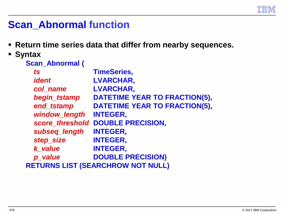
Scan_Abnormal function
Return time series data that differ from nearby sequences. Syntax
− Scan_Abnormal ( − ts TimeSeries, − ident LVARCHAR, − col_name LVARCHAR, − begin_tstamp DATETIME YEAR TO FRACTION(5), − end_tstamp DATETIME YEAR TO FRACTION(5), − window_length INTEGER, − score_threshold DOUBLE PRECISION, − subseq_length INTEGER, − step_size INTEGER, − k_value INTEGER, − p_value DOUBLE PRECISION) − RETURNS LIST (SEARCHROW NOT NULL)
© 2017 IBM Corporation479

Scan_Abnormal function ts
− The time series value for the specified primary key. ident
− A string identifier that is associated with the time series instance. col_name
− The column name in the TimeSeries data type from which to retrieve the values.
begin_stamp− The begin point of the search range.
• Can be NULL, which represents the first time series element. end_stamp
− The end point of the search range. • Can be NULL, which represents the last time series element.
window_length− The length of the sequence.
score_threshold− The abnormal score threshold. Range of values: 0.0 - 1.0.
© 2017 IBM Corporation480

Scan_Abnormal function
subseq_length− The size of the sliding window.
step_size− How far the sliding window is advanced for each candidate match.
k_value− Number of nearest neighbor sequences on which to base the abnormality
score. p_value
− The p value defined in the Lp-norm function, used in the distance calculation. Usage
− Run to find all subsequences that differ from nearby subsequences. − The sliding window of the input time series steps over the target time series. − The differences between the time series are a measure of Euclid distance. − Use to find outlier data compared to historical data or to generate real-time
alerts for current outlier data.
© 2017 IBM Corporation481

Scan_Abnormal function
Returns− A list of matches in a LIST data type that contains a SEARCHROW data type
value for each match.
© 2017 IBM Corporation482

Scan_Abnormal_Default function
Return time series data that differ from nearby sequences. Syntax
− Scan_Abnormal_Default ( − ts TimeSeries, − ident LVARCHAR, − col_name LVARCHAR, − begin_tstamp DATETIME YEAR TO FRACTION(5), − end_tstamp DATETIME YEAR TO FRACTION(5), − window_length INTEGER, − score_threshold DOUBLE PRECISION, − subseq_length INTEGER, − step_size INTEGER, − k_value INTEGER, − p_value DOUBLE PRECISION) − RETURNS LIST (SEARCHROW NOT NULL)
© 2017 IBM Corporation483

Scan_Abnormal_Default function
ts− The time series value for the specified primary key.
ident− A string identifier that is associated with the time series instance.
col_name− The column name in the TimeSeries data type from which to retrieve the
values. begin_stamp
− The begin point of the search range. • Can be NULL, which represents the first time series element.
end_stamp− The end point of the search range.
• Can be NULL, which represents the last time series element. window_length
− The length of the sequence. score_threshold
− The abnormal score threshold. Range of values: 0.0 - 1.0.
© 2017 IBM Corporation484

Scan_Abnormal_Default function
subseq_length− The size of the sliding window.
step_size− How far the sliding window is advanced for each candidate match.
k_value− The number of nearest neighbor sequences on which to base the abnormality
score. p_value
− The p value as defined in the Lp-norm function, which is used in the distance calculation.
Usage− Run to find all subsequences that differ from nearby subsequences. − The sliding window of the input time series steps over the target time series. − The differences between the time series are a measure of Euclid distance. − Use to find outlier data compared to historical data or to generate real-time
alerts for current outlier data.
© 2017 IBM Corporation485

Scan_Abnormal_Default function
Uses the same detection algorithm as the Scan_Abnormal function with the following fixed values:− step_size = 1− k_value = (window_length - subseq_length/step_size
Returns− A list of matches in a LIST data type that contains a SEARCHROW data type
value for each match.
© 2017 IBM Corporation486

Scan_DTW_Itakura_Parallelogram_Constraint function
Returns time series data that matches a pattern using dynamic time warping distance with the Itakura parallelogram constraint.
Syntax Scan_DTW_Itakura_Parallelogram_Constraint (
− ts TimeSeries, − ident LVARCHAR, − col_name LVARCHAR, − begin_tstamp DATETIME YEAR TO FRACTION(5), − end_tstamp DATETIME YEAR TO FRACTION(5), − pattern LIST (ROW (DOUBLE PRECISION) NOT
NULL), − enlarge_threshold DOUBLE PRECISION, − mconstraint_horizontal DOUBLE PRECISION, − mconstraint_vertical DOUBLE PRECISION, − dtw_threshold DOUBLE PRECISION)
RETURNS LIST (SEARCHROW NOT NULL)
© 2017 IBM Corporation487

Scan_DTW_Itakura_Parallelogram_Constraint function
ts− The time series value for the specified primary key.
ident− A string identifier that is associated with the time series instance.
col_name− The column name in the TimeSeries data type from which to retrieve the
values. begin_stamp
− The begin point of the search range. • Can be NULL, which represents the first element in the time series.
end_stamp− The end point of the search range.
• Can be NULL, which represents the last element in the time series. pattern
− Search pattern returned by the ValueAsCollection or TSGetValueListfunction.
© 2017 IBM Corporation488

Scan_DTW_Itakura_Parallelogram_Constraint function
enlarge_threshold− A number that when multiplied by the pattern length specifies the size of the
sliding window. mconstraint_horizontal
− A number that represents the mConstraint horizontal values that define a parallelogram-shaped region to restrict the DTW distance calculation.
mconstraint_vertical− A number that represents the mConstraint vertical values that define a
parallelogram-shaped region to restrict the DTW distance calculation. dtw_threshold
− A number that represents the upper bound of the DTW score. Usage
− Run to find fragments in a time series that are under the threshold, based on the DTW score with an Itakura Parallelogram constraint, with a sliding window.
Returns− A list of matches in a LIST data type that contains a SEARCHROW data type
value for each match.
© 2017 IBM Corporation489

Scan_DTW_NonConstraint function Returns matching time series sequences using dynamic time
warping without constraints. Syntax
− Scan_DTW_NonConstraint( • ts TimeSeries, • ident LVARCHAR, • col_name LVARCHAR, • begin_tstamp DATETIME YEAR TO FRACTION(5), • end_tstamp DATETIME YEAR TO FRACTION(5), • pattern LIST (ROW (DOUBLE PRECISION) NOT NULL),• enlarge_threshold DOUBLE PRECISION, • dtw_threshold DOUBLE PRECISION)
− RETURNS LIST (SEARCHROW NOT NULL)
© 2017 IBM Corporation490

Scan_DTW_NonConstraint function
ts− The time series value for the specified primary key.
ident− A string identifier that is associated with the time series instance.
col_name− The column name in the TimeSeries data type from which to retrieve the values.
begin_stamp− The begin point of the range to search.
• Can be NULL, which represents the first element in the time series. end_stamp
− The end point of the range to search. • Can be NULL, which represents the last element in the time series.
pattern− Search pattern returned by the ValueAsCollection or TSGetValueList function.
© 2017 IBM Corporation491

Scan_DTW_NonConstraint function
enlarge_threshold− A number that when multiplied by the pattern length specifies the size of the
sliding window. dtw_threshold
− A number that represents the upper bound of the DTW score. Usage
− Run to find fragments that are under the threshold based on the unconstrained DTW score in a time series using a sliding window.
Returns− A list of matches in a LIST data type that contains a SEARCHROW data type
value for each match.
© 2017 IBM Corporation492

Scan_DTW_Sakoe_Chiba_Constraint function
Returns time series data that matches a pattern using dynamic time warping distance with the Sakoe-Chiba constraint.
Syntax− Scan_DTW_Sakoe_Chiba_Constraint (
• ts TimeSeries, • ident LVARCHAR, • col_name LVARCHAR, • begin_tstamp DATETIME YEAR TO FRACTION(5), • end_tstamp DATETIME YEAR TO FRACTION(5), • pattern LIST (ROW (DOUBLE PRECISION) NOT
NULL), • enlarge_threshold DOUBLE PRECISION, • norm_mconstraint DOUBLE PRECISION, • dtw_threshold DOUBLE PRECISION)
− RETURNS LIST (SEARCHROW NOT NULL)
© 2017 IBM Corporation493

Scan_DTW_Sakoe_Chiba_Constraint function
ts− The time series value for the specified primary key.
ident− A string identifier that is associated with the time series instance.
col_name− The column name in the TimeSeries data type from which to retrieve the values.
begin_stamp− The begin point of the range to search.
• Can be NULL, which represents the first element in the time series. end_stamp
− The end point of the range to search. • Can be NULL, which represents the last element in the time series.
pattern− Search pattern returned by the ValueAsCollection or TSGetValueList function.
© 2017 IBM Corporation494

Scan_DTW_Sakoe_Chiba_Constraint function
enlarge_threshold− A number that when multiplied by the pattern length specifies the size of the
sliding window. norm_mconstraint
− A number that represents the normalized mConstraint in the Sakoe-Chiba function.
dtw_threshold− A number that represents the upper bound of the DTW score.
Usage− Run to find fragments that are under the threshold based on the DTW score
with a Sakoe-Chiba constraint in a time series using a sliding window. Returns
− A list of matches in a LIST data type that contains a SEARCHROW data type value for each match.
© 2017 IBM Corporation495

Scan_Normal_LCSS function
Matches the search pattern to the time series using the longest common subsequence formula.
Syntax− Scan_Normal_LCSS(
• ts TimeSeries, • ident LVARCHAR, • col_name LVARCHAR, • begin_tstamp DATETIME YEAR TO FRACTION(5), • end_tstamp DATETIME YEAR TO FRACTION(5), • pattern LIST (ROW (DOUBLE PRECISION) NOT
NULL),• enlarge_threshold DOUBLE PRECISION, • normalized_delta DOUBLE PRECISION, • epsilon DOUBLE PRECISION, • norm_lcss_threshold DOUBLE PRECISION)
− RETURNS LIST (SEARCHROW NOT NULL)
© 2017 IBM Corporation496

Scan_Normal_LCSS function
ts− The time series value for the specified primary key.
ident− A string identifier that is associated with the time series instance.
col_name− The column name in the TimeSeries data type from which to retrieve the values.
begin_stamp− The begin point of the search range.
• Can be NULL, which represents the first element in the time series. end_stamp
− The end point of the search range. • Can be NULL, which represents the last element in the time series.
pattern− Search pattern returned by the ValueAsCollection or TSGetValueList function.
© 2017 IBM Corporation497

Scan_Normal_LCSS function
enlarge_threshold– A number that when multiplied by the pattern length specifies the size of the
sliding window. normalized_delta
– The limit of the delta distance. epsilon
– The value of ϵ in the longest common subsequence formula. norm_lcss_threshold
– The high bound of the distance. lcss_threshold
– The high bound of the distance.
Usage– This function measures the longest common subsequence (LCSS) similarity
between the subsequences of a time series and a pattern using a sliding window, where the length of the two subsequences is not necessarily the same.
© 2017 IBM Corporation498

Scan_Normal_LCSS function
Returns− A list of matches in a LIST data type that contains a SEARCHROW data type
value for each match.
© 2017 IBM Corporation499

Scan_LCSS function
Matches the search pattern to the time series using the longest common subsequence formula.
Syntax− Scan_LCSS(
• ts TimeSeries, • ident LVARCHAR, • col_name LVARCHAR, • begin_tstamp DATETIME YEAR TO FRACTION(5), • end_tstamp DATETIME YEAR TO FRACTION(5), • pattern LIST (ROW (DOUBLE PRECISION) NOT
NULL),• enlarge_threshold DOUBLE PRECISION, • normalized_delta DOUBLE PRECISION, • epsilon DOUBLE PRECISION, • norm_lcss_threshold DOUBLE PRECISION)
− RETURNS LIST (SEARCHROW NOT NULL)
© 2017 IBM Corporation500

Scan_LCSS function
ts− The time series value for the specified primary key.
ident− A string identifier that is associated with the time series instance.
col_name− The column name in the TimeSeries data type from which to retrieve the values.
begin_stamp− The begin point of the search range.
• Can be NULL, which represents the first element in the time series. end_stamp
− The end point of the search range. • Can be NULL, which represents the last element in the time series.
pattern− Search pattern returned by the ValueAsCollection or TSGetValueList function.
© 2017 IBM Corporation501

Scan_LCSS function
enlarge_threshold– A number that when multiplied by the pattern length specifies the size of the
sliding window. normalized_delta
– The limit of the delta distance. epsilon
– The value of ϵ in the longest common subsequence formula. norm_lcss_threshold
– The high bound of the distance. lcss_threshold
– The high bound of the distance.
Usage– This function measures the longest common subsequence (LCSS) similarity
between the subsequences of a time series and a pattern using a sliding window, where the length of the two subsequences is not necessarily the same.
© 2017 IBM Corporation502

Scan_LCSS function
Returns− A list of matches in a LIST data type that contains a SEARCHROW data type
value for each match.
© 2017 IBM Corporation503

Scan_RangeQuery_LPNorm function Uses the Lp-norm function to calculate how close the search pattern
matches fragments of the time series. Syntax
− Scan_RangeQuery_LPNorm( • ts TimeSeries, • ident LVARCHAR • col_name LVARCHAR • begin_tstamp DATETIME YEAR TO FRACTION(5), • end_tstamp DATETIME YEAR TO FRACTION(5), • pattern LIST (ROW (DOUBLE PRECISION) NOT NULL), • p_value DOUBLE PRECISION, • dist_hb DOUBLE PRECISION
− ) − RETURNS LIST (SEARCHROW NOT NULL)
© 2017 IBM Corporation504

Scan_RangeQuery_LPNorm function
ts− The time series value for the specified primary key.
ident− A string identifier that is associated with the time series instance.
col_name− The column name in the TimeSeries data type from which to retrieve the values.
begin_stamp− The begin point of the search range.
• Can be NULL, which represents the first element in the time series. end_stamp
− The end point of the search range. • Can be NULL, which represents the last element in the time series.
pattern− Search pattern returned by the ValueAsCollection or TSGetValueList function.
© 2017 IBM Corporation505

Scan_RangeQuery_LPNorm function
p_value− The p value as defined in the Lp-norm function. − Must be > 0.
dist_hb− The high bound of the threshold of the Lp-norm distance.
Usage− Run to find fragments in the specified time series for the specified time range
that are under the threshold of the constraint, which is based on the Lp-normdistance that is computed with the specified pattern.
− The length of the fragments must be the same. Returns
− A list of matches in a LIST data type that contains a SEARCHROW data type value for each match.
© 2017 IBM Corporation506

Scan_RangeQuery_Pearson_Correlation function
Returns time series data that matches a pattern using a Pearson correlation.
Syntax− Scan_RangeQuery_Pearson_Correlation (
• ts TimeSeries, • ident LVARCHAR, • col_name LVARCHAR, • begin_tstamp DATETIME YEAR TO FRACTION(5), • end_tstamp DATETIME YEAR TO FRACTION(5), • pattern LIST (ROW (DOUBLE PRECISION) NOT NULL), • lower_bound DOUBLE PRECISION)
− RETURNS LIST (SEARCHROW NOT NULL)
© 2017 IBM Corporation507

Scan_RangeQuery_Pearson_Correlation function
ts− The time series value for the specified primary key.
ident− A string identifier that is associated with the time series instance.
col_name− The column name in the TimeSeries data type from which to retrieve the values.
begin_stamp− The begin point of the search range.
• Can be NULL, which represents the first element in the time series. end_stamp
− The end point of the search range. • Can be NULL, which represents the last element in the time series.
pattern− Search pattern returned by the ValueAsCollection or TSGetValueList function.
© 2017 IBM Corporation508

Scan_RangeQuery_Pearson_Correlation function
lower_bound− A number that represents the lower bound of similarity as calculated by the
Pearson Correlation function. − Range of values is 0.0 - 1.0.
Usage− Run to find fragments in a sliding windows that match the search pattern using a
Pearson Correlation function to calculate the lower bound. Returns
− A list of matches in a LIST data type that contains a SEARCHROW data type value for each match.
© 2017 IBM Corporation509

TSAFuncsTraceFile function
Sets the trace file name and path for advanced analytics functions. Syntax
− TSAFuncsTraceFile (trace_file LVARCHAR) returns INTEGER trace_file• The path and name of the trace file.
Usage− Run the TSAFuncsTraceFile function to give the trace file for advanced
analytics functions a different name and location from the default of /tmp/sessionID.trc, where sessionID is the session ID.
− You enable tracing with the TSAFuncsTraceLevel function. Returns
− 0 = The trace file name and path are set.− An error.
Example− The following statement sets the file name and path of the trace file:
• EXECUTE FUNCTION TSAFuncsTraceFile(/usr/mytrace/timeseries.trc);
© 2017 IBM Corporation510

TSAFuncsTraceLevel function
Enables tracing on advanced analytics functions. Syntax
− TSAFuncsTraceLevel('TSAF_DEBUG 1') returns INTEGER Usage
− Run the TSAFuncsTraceLevel function to enable tracing if you want to view the entry points of advanced analytics functions.
− Tracing file is named /tmp/sessionID.trc, where sessionID is the session ID. − You can change the location and name of the tracing file with the
TSAFuncsTraceFile function. Returns
− 0 = Tracing is enabled.− An error.
Example− The following statement enables tracing:
• EXECUTE FUNCTION TSAFuncsTraceLevel('TSAF_DEBUG 1');
© 2017 IBM Corporation511

TSAFuncsRelease function
Returns the version number and build date for the TimeSeries advanced analytics extension.
Syntax− TSAFuncsRelease() returns LVARCHAR;
Returns− A string with the version number and build date.
Example− The following statement returns the version number and build date:− EXECUTE FUNCTION TSAFuncsRelease();
© 2017 IBM Corporation512

TSCompute_Itakura_Parallelogram_Constraint_Dist function Calculates a similarity score for two time series sequences with the
Itakura Parallelogram constraint applied to the distance calculation.
Syntax− TSCompute_Itakura_Parallelogram_Constraint_Dist ( − sequence1 list, − sequence2 list, − mconstraint_horizontal DOUBLE PRECISION, − mconstraint_vertical DOUBLE PRECISION) − RETURNS DOUBLE PRECISION − sequence1 and sequence2
• A list of values returned by the ValueAsCollection or TSGetValueList function. − mconstraint_horizontal
• A number that represents the mConstraint horizontal values that define a parallelogram-shaped region to restrict the DTW distance calculation.
− mconstraint_vertical• A number that represents the mConstraint vertical values that define a
parallelogram-shaped region to restrict the DTW distance calculation.
© 2017 IBM Corporation513

TSCompute_Itakura_Parallelogram_Constraint_Dist function Usage
− Run the TSCompute_Itakura_Parallelogram_Constraint_Dist function to calculate the distance between two time series sequences with the Itakura Parallelogram constraint.
− The length of the sequences must be the same. Returns
− A number that represents the similarity distance between two sequences.
© 2017 IBM Corporation514

TSCompute_LCSS_Dist function
Calculates the longest common subsequence distance between two time series sequences.
Syntax– TSCompute_LCSS_Dist ( – sequence1 list, – sequence2 list, – normalize_delta DOUBLE PRECISION, – epsilon DOUBLE PRECISION) – RETURNS DOUBLE PRECISION – sequence1
• A list of values returned by the ValueAsCollection or TSGetValueList function. – sequence2
• A list of values returned by the ValueAsCollection or TSGetValueList function. – normalized_delta
• The limit of the delta distance. – epsilon
• The value of ϵ in the longest common subsequence formula.
© 2017 IBM Corporation515

TSCompute_LCSS_Dist function
Usage− The TSCompute_LCSS_Dist function returns the actual distance.
Returns− A number that represents the difference between two sequences.
© 2017 IBM Corporation516

TSCompute_Normalized_LCSS_Dist function
Calculates the longest common subsequence distance between two time series sequences.
Syntax– TSCompute_Normalized_LCSS_Dist ( – sequence1 list, – sequence2 list, – normalize_delta DOUBLE PRECISION, – epsilon DOUBLE PRECISION) – RETURNS DOUBLE PRECISION – sequence1
• A list of values returned by the ValueAsCollection or TSGetValueList function. – sequence2
• A list of values returned by the ValueAsCollection or TSGetValueList function. – normalized_delta
• The limit of the delta distance. – epsilon
• The value of ϵ in the longest common subsequence formula.
© 2017 IBM Corporation517

TSCompute_Normalized_LCSS_Dist function
Usage− Run to use the longest common subsequence algorithm to calculate the
distance between two time series sequences. − Returns the distance as a value 0.0 - 1.0.
Returns− A number that represents the difference between two sequences.
© 2017 IBM Corporation518

TSCompute_LP_Dist function
Uses the Lp-norm function to calculate how closely the two time series sequences match.
Syntax− TSCompute_LP_Dist ( sequence1 list, sequence2 list, p_value DOUBLE
PRECISION) − RETURNS DOUBLE PRECISION − sequence1
• A list of values returned by the ValueAsCollection or TSGetValueList function. − sequence2
• A list of values returned by the ValueAsCollection or TSGetValueList function. − p_value
• The p value as defined in the Lp-norm function. • Must be greater than 0.
© 2017 IBM Corporation519

TSCompute_LP_Dist function
Usage− Run to calculate the distance between two time series sequences with the Lp-
norm function. − The length of the sequences must be the same.
Returns− A number that represents the difference between two sequences.
© 2017 IBM Corporation520

TSCompute_NonConstraint_Dist function
Calculates the DTW distance between two time series sequences without constraints.
Syntax− TSCompute_NonConstraint_Dist (sequence1 list, sequence2 list) − RETURNS DOUBLE PRECISION − sequence1
• A list of values returned by the ValueAsCollection or TSGetValueList function. − sequence2
• A list of values returned by the ValueAsCollection or TSGetValueList function. Usage
− Run to calculate the distance between two time series sequences without constraints.
− The length of the sequences must be the same. Returns
− A number that represents the distance between two sequences.
© 2017 IBM Corporation521

TSCompute_Sakoe_Chiba_Constraint_Dist function
Calculates a similarity score for two time series sequences with the Sakoe Chiba constraint.
Syntax− TSCompute_Sakoe_Chiba_Constraint_Dist − ( − sequence1 list, − sequence2 list, − norm_mconstraint DOUBLE PRECISION− ) − RETURNS DOUBLE PRECISION − sequence1
• A list of values that is returned by the ValueAsCollection or TSGetValueListfunction.
− sequence2• A list of values that is returned by the ValueAsCollection or TSGetValueList
function. − norm_mconstraint
• A number that represents the normalized mConstraint in the Sakoe-Chiba function.
© 2017 IBM Corporation522

TSCompute_Sakoe_Chiba_Constraint_Dist function
Usage− Run the TSPearson_Correlation_Score function to calculate the similarity
distance between two time series sequences, restricted by the Sakoe-Chiba constraint.
− The length of the sequences must be the same. Returns
− A number that represents the distance between the two time series sequences.
© 2017 IBM Corporation523

TSGetValueList function
Converts a string into a list of values useful as input to an advanced analytics function.
Syntax− TSGetValueList (value_string LVARCHAR) − RETURNS LIST (ROW (value DOUBLE PRECISION) NOT NULL) − TSGetValueList (value_string LVARCHAR, num_elements INTEGER) − RETURNS LIST (ROW (value DOUBLE PRECISION) NOT NULL) − value_string
• A character string that represents a list of data values.− num_elements
• A positive integer representing the number of input values to use from the start of the input string.
Usage− Run this to return a search pattern usable as input to an advanced analytics
function. − You can run the TSGetValueList function within an advanced analytics function
as the pattern argument.
© 2017 IBM Corporation524

TSGetValueList function
Returns− A list of row types that have a DOUBLE PRECISION field.
© 2017 IBM Corporation525

TSPearson_Correlation_Score function
Generates a Pearson correlation score for two time series sequences. Syntax
− TSPearson_Correlation_Score ( sequence1 list, sequence2 list) − RETURNS DOUBLE PRECISION − sequence1
• A list of values that is returned by the ValueAsCollection or TSGetValueListfunction.
− sequence2• A list of values that is returned by the ValueAsCollection or TSGetValueList
function. Usage
− Run to calculate the Pearson correlation coefficient between two time series sequences.
− The length of the sequences must be the same. Returns
− Number, between 0.0 - 1.0, representing the Pearson correlation coefficient.
© 2017 IBM Corporation526

ValueAsCollection function
Returns a search pattern useful as input to an advanced analytics function
Syntax− ValueAsCollection ( − ts TimeSeries, − begin_tstamp DATETIME YEAR TO FRACTION(5), − end_tstamp DATETIME YEAR TO FRACTION(5), − col_name LVARCHAR− ) − RETURNS LIST (ROW (value DOUBLE PRECISION) NOT NULL) − ValueAsCollection ( − ts TimeSeries, − begin_tstamp DATETIME YEAR TO FRACTION(5), − end_tstamp DATETIME YEAR TO FRACTION(5), − col_num INTEGER− ) RETURNS LIST (ROW (value DOUBLE PRECISION) NOT NULL
© 2017 IBM Corporation527

ValueAsCollection function
Usage− Returns a search pattern that you can use as input to an advanced analytics
function • A search pattern is the list of values from the specified column in the TimeSeries data
type for the specified time range. − You can run this function within the analytics function as the pattern argument.
Returns− A list of row types that have a DOUBLE PRECISION field.
© 2017 IBM Corporation528

Appendix E – GSKit Installation
B
© 2017 IBM Corporation

GSKit
Normally installed with Informix Dynamic Server as part of the installation process and enabled by default for both Linux/Unix and Windows.
Separate install instructions for:– AIX– LINUX– Solaris– Windows
© 2017 IBM Corporation530