Informed Search - University of Waterloopami.uwaterloo.ca/~basir/ECE457/week3.pdf · Informed...
47
E&CE 457 Applied Artificial Intelligence Page 1 Informed Search Uninformed search is systematic but inefficient. Would like to use additional knowledge such that better nodes are considered for expansion and exploration first. In terms of pseudo-code, we want to order the open queue. We will introduce an evaluation function f(n) that indicates the desirability of considering node n next for exploration and expansion. Nodes with a better f(n) are always considered first. How should we compute f(n) ???
Transcript of Informed Search - University of Waterloopami.uwaterloo.ca/~basir/ECE457/week3.pdf · Informed...

E&CE 457 Applied Artificial Intelligence Page 1
Informed Search
Uninformed search is systematic but inefficient.
Would like to use additional knowledge such that better nodes are considered for expansion and exploration first.
In terms of pseudo-code, we want to order the open queue.
We will introduce an evaluation function f(n) that indicates the desirability of considering node n next for exploration and expansion.
Nodes with a better f(n) are always considered first.
How should we compute f(n) ???

E&CE 457 Applied Artificial Intelligence Page 2
Recall Uniform Cost Search
UCS orders the open queue according to the path cost g(n).
Path cost is distance from root to state n.
So, UCS uses an evaluation function f(n) = g(n).
The path cost g(n) only accounts for cost to reach n.
UCS is NOT goal directed/oriented.
Would also like to consider the cost from state n to the goal.

E&CE 457 Applied Artificial Intelligence Page 3
Being Goal Oriented
Would like f(n) to include a measure of the cost to goal.
Use what’s called a heuristic function h(n). an estimate of the cost from the current state to goal.
Two ideas/approaches; always try to expand nodes that are: Estimated to be closest to goal. f(n) = h(n) (Greedy Best First Search)
On least cost path from root, through current state, to the goal. f(n) = g(n) + h(n) (A* Search)
Heuristic function h(n) is: Only an estimate (whereas path cost g(n) is exact). Equal to zero when at the goal.

E&CE 457 Applied Artificial Intelligence Page 4
Greedy Best First Search
Always explores and expands the node judged to be closest to goal.
So, uses f(n) = h(n) and ignores the path cost g(n) entirely.
Consider it to be the complement of UCS.

E&CE 457 Applied Artificial Intelligence Page 5
Illustration of Greedy Best First Search
Consider wanting to find a path from (6,1) to (3,6), but we have obstacles.
Let the estimate of distance to goal be the manhattan distance between the current position (x,y) and the goal (dstx,dsty); i.e., h(n) = |x-dstx|+|y-dsty|.
NOTE: our heuristic does not look at obstacles (problem relaxation, more Friday)
6 5 4 3 4 5 6 7 8 9
5 4 3 2 3 4 5 6 7 8
4 3 2 1 2 3 4 5 6 7
3 2 1 0 1 4 5 6
4 3 4 5 6 7
5 4 2 3 4 5 6 7 8
6 5 3 4 8 9
7 6 4 5 9 10
8 7 6 5 6 7 8 9 10 11
9 8 7 6 7 8 9 10 11 12
Distances to goal h(n)
E&CE 457 Applied Artificial Intelligence Page 6
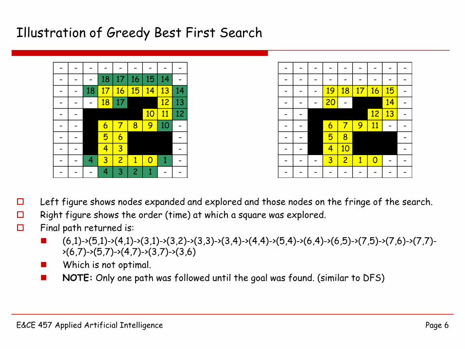
Illustration of Greedy Best First Search
Left figure shows nodes expanded and explored and those nodes on the fringe of the search.
Right figure shows the order (time) at which a square was explored.
Final path returned is:
(6,1)->(5,1)->(4,1)->(3,1)->(3,2)->(3,3)->(3,4)->(4,4)->(5,4)->(6,4)->(6,5)->(7,5)->(7,6)->(7,7)->(6,7)->(5,7)->(4,7)->(3,7)->(3,6)
Which is not optimal.
NOTE: Only one path was followed until the goal was found. (similar to DFS)
- - - - - - - - -
- - - - - - - - -
- - - 19 18 17 16 15 -
- - - 20 - 14 -
- - 12 13 -
- - 6 7 9 11 - -
- - 5 8 -
- - 4 10 -
- - - 3 2 1 0 - -
- - - - - - - - -
- - - - - - - - -
- - - 18 17 16 15 14 -
- - 18 17 16 15 14 13 14
- - - 18 17 12 13
- - 10 11 12
- - 6 7 8 9 10 -
- - 5 6 -
- - 4 3 -
- - 4 3 2 1 0 1 -
- - - 4 3 2 1 - -

E&CE 457 Applied Artificial Intelligence Page 7
Queue Contents
Can illustrate the contents of the open and closed queue. Note that:
Goal appears at the head of the open queue just prior to termination.
Open queue contains the fringe nodes upon termination.
1 open [(6,1,8.0)]
closed
2 open [(5,1,7.0)][(6,0,9.0)][(7,1,9.0)]
closed [(6,1,8.0)]
3 open [(4,1,6.0)][(5,0,8.0)][(6,0,9.0)][(7,1,9.0)]
closed [(6,1,8.0)][(5,1,7.0)]
4 open [(3,1,5.0)][(4,2,5.0)][(4,0,7.0)][(5,0,8.0)][(6,0,9.0)][(7,1,9.0)]
closed [(6,1,8.0)][(5,1,7.0)][(4,1,6.0)]
5 open [(3,2,4.0)][(4,2,5.0)][(2,1,6.0)][(3,0,6.0)][(4,0,7.0)][(5,0,8.0)][(6,0,9.0)][(7,1,9.0)]
closed [(6,1,8.0)][(5,1,7.0)][(4,1,6.0)][(3,1,5.0)]
6 open [(3,3,3.0)][(4,2,5.0)][(2,1,6.0)][(3,0,6.0)][(4,0,7.0)][(5,0,8.0)][(6,0,9.0)][(7,1,9.0)]
closed [(6,1,8.0)][(5,1,7.0)][(4,1,6.0)][(3,1,5.0)][(3,2,4.0)]
7 open [(3,4,2.0)][(4,3,4.0)][(4,2,5.0)][(2,1,6.0)][(3,0,6.0)][(4,0,7.0)][(5,0,8.0)][(6,0,9.0)][(7,1,9.0)]
closed [(6,1,8.0)][(5,1,7.0)][(4,1,6.0)][(3,1,5.0)][(3,2,4.0)][(3,3,3.0)]
8 open [(4,4,3.0)][(4,3,4.0)][(4,2,5.0)][(2,1,6.0)][(3,0,6.0)][(4,0,7.0)][(5,0,8.0)][(6,0,9.0)][(7,1,9.0)]
closed [(6,1,8.0)][(5,1,7.0)][(4,1,6.0)][(3,1,5.0)][(3,2,4.0)][(3,3,3.0)][(3,4,2.0)]
9 open [(4,3,4.0)][(5,4,4.0)][(4,2,5.0)][(2,1,6.0)][(3,0,6.0)][(4,0,7.0)][(5,0,8.0)][(6,0,9.0)][(7,1,9.0)]
closed [(6,1,8.0)][(5,1,7.0)][(4,1,6.0)][(3,1,5.0)][(3,2,4.0)][(3,3,3.0)][(3,4,2.0)][(4,4,3.0)]
10 open [(5,4,4.0)][(4,2,5.0)][(2,1,6.0)][(3,0,6.0)][(4,0,7.0)][(5,0,8.0)][(6,0,9.0)][(7,1,9.0)]
closed [(6,1,8.0)][(5,1,7.0)][(4,1,6.0)][(3,1,5.0)][(3,2,4.0)][(3,3,3.0)][(3,4,2.0)][(4,4,3.0)][(4,3,4.0)]
11 open [(4,2,5.0)][(6,4,5.0)][(2,1,6.0)][(3,0,6.0)][(4,0,7.0)][(5,0,8.0)][(6,0,9.0)][(7,1,9.0)]
closed [(6,1,8.0)][(5,1,7.0)][(4,1,6.0)][(3,1,5.0)][(3,2,4.0)][(3,3,3.0)][(3,4,2.0)][(4,4,3.0)][(4,3,4.0)][(5,4,4.0)]

E&CE 457 Applied Artificial Intelligence Page 8
Queue Contents cont’d
12 open [(6,4,5.0)][(2,1,6.0)][(3,0,6.0)][(4,0,7.0)][(5,0,8.0)][(6,0,9.0)][(7,1,9.0)]
closed [(6,1,8.0)][(5,1,7.0)][(4,1,6.0)][(3,1,5.0)][(3,2,4.0)][(3,3,3.0)][(3,4,2.0)][(4,4,3.0)][(4,3,4.0)][(5,4,4.0)]
[(4,2,5.0)]
13 open [(6,5,4.0)][(2,1,6.0)][(3,0,6.0)][(7,4,6.0)][(4,0,7.0)][(5,0,8.0)][(6,0,9.0)][(7,1,9.0)]
closed [(6,1,8.0)][(5,1,7.0)][(4,1,6.0)][(3,1,5.0)][(3,2,4.0)][(3,3,3.0)][(3,4,2.0)][(4,4,3.0)][(4,3,4.0)][(5,4,4.0)]
[(4,2,5.0)][(6,4,5.0)]
14 open [(7,5,5.0)][(2,1,6.0)][(3,0,6.0)][(7,4,6.0)][(4,0,7.0)][(5,0,8.0)][(6,0,9.0)][(7,1,9.0)]
closed [(6,1,8.0)][(5,1,7.0)][(4,1,6.0)][(3,1,5.0)][(3,2,4.0)][(3,3,3.0)][(3,4,2.0)][(4,4,3.0)][(4,3,4.0)][(5,4,4.0)]
[(4,2,5.0)][(6,4,5.0)][(6,5,4.0)]
15 open [(7,6,4.0)][(2,1,6.0)][(3,0,6.0)][(7,4,6.0)][(8,5,6.0)][(4,0,7.0)][(5,0,8.0)][(6,0,9.0)][(7,1,9.0)]
closed [(6,1,8.0)][(5,1,7.0)][(4,1,6.0)][(3,1,5.0)][(3,2,4.0)][(3,3,3.0)][(3,4,2.0)][(4,4,3.0)][(4,3,4.0)][(5,4,4.0)]
[(4,2,5.0)][(6,4,5.0)][(6,5,4.0)][(7,5,5.0)]
16 open [(7,7,5.0)][(8,6,5.0)][(2,1,6.0)][(3,0,6.0)][(7,4,6.0)][(8,5,6.0)][(4,0,7.0)][(5,0,8.0)][(6,0,9.0)][(7,1,9.0)]
closed [(6,1,8.0)][(5,1,7.0)][(4,1,6.0)][(3,1,5.0)][(3,2,4.0)][(3,3,3.0)][(3,4,2.0)][(4,4,3.0)][(4,3,4.0)][(5,4,4.0)]
[(4,2,5.0)][(6,4,5.0)][(6,5,4.0)][(7,5,5.0)][(7,6,4.0)]
17 open [(6,7,4.0)][(8,6,5.0)][(2,1,6.0)][(3,0,6.0)][(7,4,6.0)][(8,5,6.0)][(7,8,6.0)][(8,7,6.0)][(4,0,7.0)][(5,0,8.0)]
[(6,0,9.0)][(7,1,9.0)]
closed [(6,1,8.0)][(5,1,7.0)][(4,1,6.0)][(3,1,5.0)][(3,2,4.0)][(3,3,3.0)][(3,4,2.0)][(4,4,3.0)][(4,3,4.0)][(5,4,4.0)]
[(4,2,5.0)][(6,4,5.0)][(6,5,4.0)][(7,5,5.0)][(7,6,4.0)][(7,7,5.0)]
18 open [(5,7,3.0)][(8,6,5.0)][(6,8,5.0)][(2,1,6.0)][(3,0,6.0)][(7,4,6.0)][(8,5,6.0)][(7,8,6.0)][(8,7,6.0)][(4,0,7.0)]
[(5,0,8.0)][(6,0,9.0)][(7,1,9.0)]
closed [(6,1,8.0)][(5,1,7.0)][(4,1,6.0)][(3,1,5.0)][(3,2,4.0)][(3,3,3.0)][(3,4,2.0)][(4,4,3.0)][(4,3,4.0)][(5,4,4.0)]
[(4,2,5.0)][(6,4,5.0)][(6,5,4.0)][(7,5,5.0)][(7,6,4.0)][(7,7,5.0)][(6,7,4.0)]
19 open [(4,7,2.0)][(5,8,4.0)][(8,6,5.0)][(6,8,5.0)][(2,1,6.0)][(3,0,6.0)][(7,4,6.0)][(8,5,6.0)][(7,8,6.0)][(8,7,6.0)]
[(4,0,7.0)][(5,0,8.0)][(6,0,9.0)][(7,1,9.0)]
closed [(6,1,8.0)][(5,1,7.0)][(4,1,6.0)][(3,1,5.0)][(3,2,4.0)][(3,3,3.0)][(3,4,2.0)][(4,4,3.0)][(4,3,4.0)][(5,4,4.0)]
[(4,2,5.0)][(6,4,5.0)][(6,5,4.0)][(7,5,5.0)][(7,6,4.0)][(7,7,5.0)][(6,7,4.0)][(5,7,3.0)]
20 open [(3,7,1.0)][(4,6,1.0)][(4,8,3.0)][(5,8,4.0)][(8,6,5.0)][(6,8,5.0)][(2,1,6.0)][(3,0,6.0)][(7,4,6.0)][(8,5,6.0)]
[(7,8,6.0)][(8,7,6.0)][(4,0,7.0)][(5,0,8.0)][(6,0,9.0)][(7,1,9.0)]
closed [(6,1,8.0)][(5,1,7.0)][(4,1,6.0)][(3,1,5.0)][(3,2,4.0)][(3,3,3.0)][(3,4,2.0)][(4,4,3.0)][(4,3,4.0)][(5,4,4.0)]
[(4,2,5.0)][(6,4,5.0)][(6,5,4.0)][(7,5,5.0)][(7,6,4.0)][(7,7,5.0)][(6,7,4.0)][(5,7,3.0)][(4,7,2.0)]
21 open [(3,6,0.0)][(4,6,1.0)][(3,8,2.0)][(2,7,2.0)][(4,8,3.0)][(5,8,4.0)][(6,8,5.0)][(8,6,5.0)][(2,1,6.0)][(3,0,6.0)]
[(7,4,6.0)][(8,5,6.0)][(7,8,6.0)][(8,7,6.0)][(4,0,7.0)][(5,0,8.0)][(6,0,9.0)][(7,1,9.0)]
closed [(6,1,8.0)][(5,1,7.0)][(4,1,6.0)][(3,1,5.0)][(3,2,4.0)][(3,3,3.0)][(3,4,2.0)][(4,4,3.0)][(4,3,4.0)][(5,4,4.0)]
[(4,2,5.0)][(6,4,5.0)][(6,5,4.0)][(7,5,5.0)][(7,6,4.0)][(7,7,5.0)][(6,7,4.0)][(5,7,3.0)][(4,7,2.0)][(3,7,1.0)]

E&CE 457 Applied Artificial Intelligence Page 9
Performance of Greedy Best First Search
Resembles DFS in that it follows a single path until it hits a dead end (and backs up … false starts).
Optimal? NO Can get stuck going down an incorrect path.
Complete? NO (in theory) Can get stuck going down an infinite path.
Time Complexity? O(bm) Worst case: must expand all nodes for a tree of depth m.
Space Complexity? O(bm) Worst case: must maintain all nodes for a tree of depth m (since it back-tracks
and jumps around* in the search tree).
However, like DFS, in the best case (with a good h(n)) it can be efficient.

E&CE 457 Applied Artificial Intelligence Page 10
A* Search
Uniform cost search orders the queue according to the path cost g(n).
Optimal, complete, but inefficient in time and space.
Greedy best first search orders the queue using the heuristic cost h(n).
Not optimal, not complete (in theory) but efficient and directed (with good heuristic … what makes a good heuristic?).
Idea behind A* is to combine the two strategies; Use an evaluation function f(n) = g(n) + h(n) to order the nodes to be explored.
f(n) measures the cheapest total estimated cost from the initial state to the goal state passing through the current state n.*
The resulting search is both optimal and complete assuming certain conditions on the heuristic cost h(n).
Since we are goal oriented, we find that, in practice, the time and space complexity is reduced (but not necessarily).

E&CE 457 Applied Artificial Intelligence Page 11
Issues In Using f(n) = g(n)+h(n) [Case 1]
When expanding a new node, we need to consider queue management.
Case 1: new node, n, expanded is not currently in the open or closed queue.
This is the only/first path found to node n.
Compute g(n), h(n) and f(n) and insert node n into the open queue. g(n)
n
initial
h(n)

E&CE 457 Applied Artificial Intelligence Page 12
Issues In Using f(n) = g(n)+h(n) [Case 2]
When expanding a new node, we need to consider queue management.
CASE 2: expanded node already in open queue.
We must have found a new path to node n.
It might be possible that g(new_path) < g(old_path). Of course, h(n) is the same.
This means we have a better overall path going through node n, so we replace the entry on the open queue with the new path if it is better.
g(old_path)
n
initial
h(n)
old path (in
OPEN)new path
g(new_path)
E&CE 457 Applied Artificial Intelligence Page 13
Issues In Using f(n) = g(n)+h(n) [Case 3]
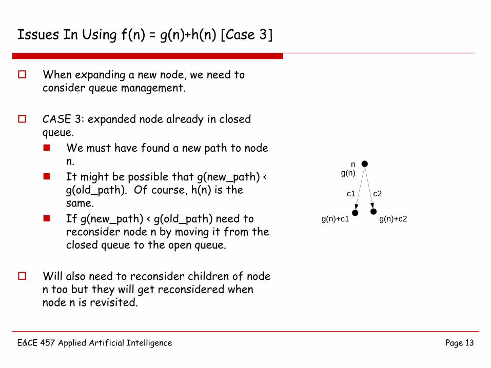
When expanding a new node, we need to consider queue management.
CASE 3: expanded node already in closed queue.
We must have found a new path to node n.
It might be possible that g(new_path) < g(old_path). Of course, h(n) is the same.
If g(new_path) < g(old_path) need to reconsider node n by moving it from the closed queue to the open queue.
Will also need to reconsider children of node n too but they will get reconsidered when node n is revisited.
g(n)n
c1
g(n)+c1
c2
g(n)+c2

E&CE 457 Applied Artificial Intelligence Page 14
Pseudo-code for A* Search
1. open_queue.insert(init_state); closed_queue.clear();
2. while (open_queue.size() != 0) {
3. curr_state = open_queue.remove_front();
4. if (is_goal(curr_state)) { return success; } // and solution
5. closed_queue.insert(curr_state);
6. child = expand(curr_state);
7. for (i = 1 ; i <= child.size() ; i++) {
8. compute_h(child[i]);
9. compute_g(child[i]) = g(curr_state) + action_cost;
10. if (open_queue.find(child[i])) {
11. if (g(child_in_open) > g(child[i])) {
12. replace_child_on_open;
13. } else ; // discard new path.
14. } else if (closed_queue.find(child[i])) {
15. if (g(Child_in_closed) > g(child[i])) {
16. closed_queue.remove(child[i]);
17. open_queue.enqueue(child[i]);
18. } else ; // discard new path.
19. } else { open_queue.enqueue(Child[i]); } // first visit.
20. }
21. sort(open_queue); // sort using f(n)=g(b)+h(n)
22. }
23. return failure; // no solution found.

E&CE 457 Applied Artificial Intelligence Page 15
Illustration of A* Search
Consider wanting to find a path from (6,1) to (3,6), but we have obstacles. Let h(n) be the manhattan distance from current position (x,y) to the goal .
Clearly admissible, since it is the straight path w/o obstacles (more on admissibility later). Let g(n) be the distance traveled from initial position to (x,y).
Solution returned by A* is: (6,1)->(5,1)->(4,1)->(3,1)->(2,1)->(1,1)->(1,2)->(1,3)->(1,4)->(1,5)->(1,6)->(2,6)->(3,6) which is optimal!
6 5 4 3 4 5 6 7 8 9
5 4 3 2 3 4 5 6 7 8
4 3 2 1 2 3 4 5 6 7
3 2 1 0 1 4 5 6
4 3 4 5 6 7
5 4 2 3 4 5 6 7 8
6 5 3 4 8 9
7 6 4 5 9 10
8 7 6 5 6 7 8 9 10 11
9 8 7 6 7 8 9 10 11 12
Distances to goal h(n)

E&CE 457 Applied Artificial Intelligence Page 16
Illustration of A* Search
Left figure shows g(n); Right figure shows h(n) (only for nodes expanded).
Can add values together to determine f(n).
Distances to goal h(n)
- - - - - - - - - -
- - - - - - - - - -
- 11 12 - - - - - 8 -
11 10 11 12 - 8 7 8
10 9 8 9 6 7
9 8 6 5 6 7 8 5 6
8 7 5 4 4 5
7 6 4 3 3 4
6 5 4 3 2 1 0 1 2 3
- 6 5 4 3 2 1 2 3 -
- - - - - - - - - -
- - - - - - - - - -
- 3 2 - - - - - 6 -
3 2 1 0 - 4 5 6
4 3 4 5 6 7
5 4 2 3 4 5 6 7 8
6 5 3 4 8 9
7 6 4 5 9 10
8 7 6 5 6 7 0 9 10 11
- 8 7 6 7 8 9 10 11 -
Distances from initial g(n)

E&CE 457 Applied Artificial Intelligence Page 17
Illustration of A* Search
Left figure shows nodes expanded and explored and those nodes on the fringe of the search.
Right figure shows the order (time) at which a square was explored.
Searches more than greedy best first search, but is optimal.
At end of search: open queue has 20 nodes, closed queue has 34 nodes.
cf. Greedy search: 17 nodes in open queue, 20 in closed (faster, not optimal result!)
- - - - - - - - - -
- - - - - - - - - -
- 11 12 - - - - - 8 -
11 10 11 12 - 8 7 8
10 9 8 9 6 7
9 8 6 5 6 7 8 5 6
8 7 5 4 4 5
7 6 4 3 3 4
6 5 4 3 2 1 0 1 2 3
- 6 5 4 3 2 1 2 3 -
- - - - - - - - - -
- - - - - - - - - -
- - - - - - - - - -
- 32 33 34 - - 31 -
- 30 24 - 29 -
- 28 9 8 16 21 - 27 -
- 26 7 6 25 -
- 23 5 4 22 -
- 19 14 3 2 1 0 11 18 -
- - 20 15 13 12 10 17 - -
E&CE 457 Applied Artificial Intelligence Page 18
Illustration of A* Search (Compare to breadth first search)
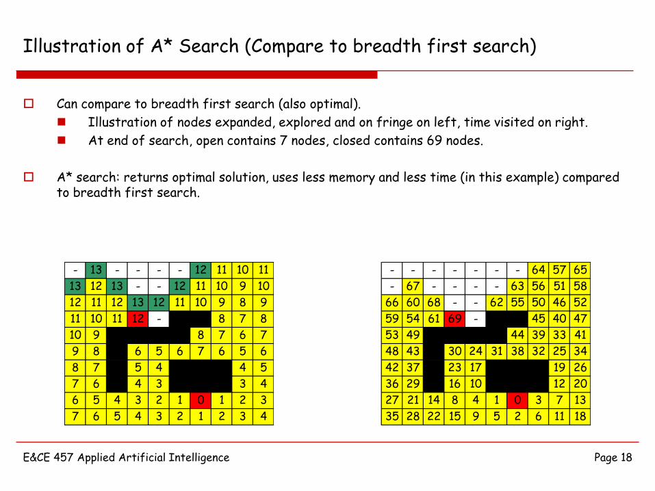
Can compare to breadth first search (also optimal).
Illustration of nodes expanded, explored and on fringe on left, time visited on right.
At end of search, open contains 7 nodes, closed contains 69 nodes.
A* search: returns optimal solution, uses less memory and less time (in this example) compared to breadth first search.
- 13 - - - - 12 11 10 11
13 12 13 - - 12 11 10 9 10
12 11 12 13 12 11 10 9 8 9
11 10 11 12 - 8 7 8
10 9 8 7 6 7
9 8 6 5 6 7 6 5 6
8 7 5 4 4 5
7 6 4 3 3 4
6 5 4 3 2 1 0 1 2 3
7 6 5 4 3 2 1 2 3 4
- - - - - - - 64 57 65
- 67 - - - - 63 56 51 58
66 60 68 - - 62 55 50 46 52
59 54 61 69 - 45 40 47
53 49 44 39 33 41
48 43 30 24 31 38 32 25 34
42 37 23 17 19 26
36 29 16 10 12 20
27 21 14 8 4 1 0 3 7 13
35 28 22 15 9 5 2 6 11 18

E&CE 457 Applied Artificial Intelligence Page 19
Illustration of A* Search (Compare to depth first search)
Can compare to depth first search (not optimal).
Illustration of nodes expanded, explored and on fringe on left, time visited on right.
At end of search, open contains 29 nodes, closed contains 37 nodes.
Returned solution has length 35!
A* search: returns optimal solution, uses less memory and less time (in this example) compared to depth first search.
- - - - - - - 13 12 11
- - - - - - - 14 - 10
- - - - - - - 15 - 9
- 35 36 37 - 16 - 8
- 34 - 17 - 7
- 33 - 21 20 19 18 - 6
- 32 - 22 - 5
- 31 - 23 - 4
- 30 29 - 24 - 0 1 2 3
- - 28 27 25 26 - - - -

E&CE 457 Applied Artificial Intelligence Page 20
Optimality of A* Search - Heuristic Function Admissibility
Optimality depends on h(n).
The heuristic cost h(n) is said to be admissible if it never overestimates the actual cost from node n to the goal.
If h(n) never overestimates, then f(n) never overestimates true cost to goal through node n.
Admissibility guarantees optimality! Sketch of proof:
Let f* be optimal cost to reach the goal, and G2 be a discovered goal with f(G2) > f*.
Consider a fringe node n along the path to the optimal solution. If h(n) admissible, then f(n) = g(n)+h(n) <= f*.
Also, f(n) <= f* < f(G2).
A* expands lowest cost nodes first, so reaching G2 implies f(G2)<= f(n) and we have a contradiction.
With h(n) admissible, we must expand any node n along the optimal path first, and this includes the optimal goal node itself.
Even without admissibility, we might still get a good search, it just won’t necessarily be optimal.

E&CE 457 Applied Artificial Intelligence Page 21
Completeness of A* Search
A* expands nodes with f(n) < f*, and possibly some nodes with f(n)=f* on the fringe before reaching the goal.
Therefore, we will eventually find the goal (complete).
Two reasons for failure:
infinite branching factor,
path with finite path cost but infinitely long.

E&CE 457 Applied Artificial Intelligence Page 22
Monotonicity of Heuristic Functions
Relates to queue management (from Wed.) and the need to re-consider nodes already in the open and closed queue when rediscovered.
Monotonicity (or consistency) means that for every node n and each of its children, the estimated cost h(n) is never greater than the cost h(child(n)) plus the action of getting to child(n).
h(n) ≤ h( child(n) ) + cost( n → child(n) )
With some mathematical arrangements:
f(n) = h(n) + g(n)
≤ h( child(n) ) + cost( n → child(n) ) + g(n)
= h( child(n) ) + g( child(n) )
= f( child(n) )
So, f(n) never decreases as we approach the goal.
Monotonicity guarantees that states are always visited by the cheapest path first; no need to check if subsequent paths are better than first.
h(n)
h(child(n))
n
child(n)
action_cost

E&CE 457 Applied Artificial Intelligence Page 23
Visualization of A* Search
Uniform cost expands in “circular” cost contours (h(n) = 0).
A* search elongates and rotates contours towards the goal. More narrow and elongated the better h(n) is. More directed!
A
Z
O
S
T
L
M
D
C
R
F
P B
G
U
V
I
N
uniform cost contours
A* search contours
goal

E&CE 457 Applied Artificial Intelligence Page 24
Informedness of Heuristic Functions
One heuristic function might be better than another for a given problem!
Informedness: For two admissible heuristic functions, h1 & h2:
if h2(n) >= h1(n), then h2(n) is more informed than h1(n). (alternatively say that h2(n) dominates h1(n) ).
More informedness implies fewer expanded states (as in previous slide).

E&CE 457 Applied Artificial Intelligence Page 25
Informedness of Heuristic Functions
A* will consider all nodes with f(n) < f*, and possibly some on the contour of f(n) = f* before finding the goal state.
Since h2(n) >= h1(n), nodes expanded by h2(n) will be expanded by h1(n). The opposite is not true
=> not all nodes expanded by h1(n) will be expanded by h2(n).*
=> h2(n) will expand fewer nodes!
Can also think of it as follows:
Assume n expanded by h2(n) but not h1(n) … implies that f2(n) < f1(n).
But, f2(n) = h2(n)+g(n) and f1(n) = h1(n) + g(n) … implies that f2(n) ≥ f1(n) since h2(n) ≥ h1(n).
→ contradiction*
Always best to pick h(n) large (but admissible).

E&CE 457 Applied Artificial Intelligence Page 26
Creation of Heuristic Functions
How to choose a heuristic function for a problem? Sometimes obvious, other times not due to constraints of the problem.
Can invent a heuristic function using a problem relaxation.
Leave out constraints and get an easier problem.
Solution to original problem solves relaxation, but not visa-versa.*
Admissible heuristic function for relaxation is admissible for original. Solution to original problem solves the relaxed problem.
=> solution must be at least as expensive and the relaxed solution.*
=> h(n) for relaxed problem is <= cost in original problem.
Can also have different heuristics and always choose the best one:

E&CE 457 Applied Artificial Intelligence Page 27
Example of Heuristic Functions
Consider the 8-puzzle and a verbal description of a move:
“Tile can move from location A to location B if A,B are adjacent and B is blank.
Consider several relaxations of this verbal description:
“I’m confused”
=> h1(n) = 0 (BFS)
“Tile can move from location A to location B”
=> h2(n) = number of tiles out of place.
“Tile can move from location A to location B if A,B adjacent”
=> h3(n) = sum of distance of tiles from goal locations.
Note: h1(n) <= h2(n) <= h3(n) <= h*(n).
h1(init_state) = 0.
h2(init_state) = 1+1+1+1+1+1+1+1=8
h3(init_state) = 2+3+3+2+3+1+1+1=16
5
8
7
6
3 2
1
4
Initial State
5
876
321
4
Goal State

E&CE 457 Applied Artificial Intelligence Page 28
Iterative Deepening A* Search
A* Search can still generate a lot of nodes (won’t consider exact complexity).
Iterative Deepening A* (IDA*):
Use iterative deepening (each iteration is limited DFS), but use f(n) costs rather than depth to limit search.
Examines all nodes within a certain cost contour using DFS.
If no solution, increase cost cutoff to the next smallest f(n), where b is a node on the fringe.
Complete and optimal like A*, but memory requirements of DFS.
Can perform poorly if small action costs (small steps each iteration).

E&CE 457 Applied Artificial Intelligence Page 29
Game playing
One of the earliest AI problems tackled as games seemed to require intelligence.
At least 4 attempts at chess alone by 1950 (Zuse, Shannon, Wiener & Turing)
Computers better than humans at checkers, Othello.
Games are (usually) well defined; e.g.,
Board games have well-defined board configurations.
Legal movements are well-defined.
Games definitely require heuristics; usually too hard to solve such problems using an exhaustive approach
E.g., chess:
Well defined: 8x8 board, pieces move in specific ways.
Has an average branching factor of ~35,
Average game lasts for ~50 moves per player,
Implies a search tree with 35100 nodes!

E&CE 457 Applied Artificial Intelligence Page 30
Adversarial search
Regular search heuristics are not appropriate for games due to involvement of an opponent (adversary).
We don’t have control over all of the movements (e.g., in a two-player game, we only have control over half of the moves)
Can’t really search for an “optimal solution”
E.g. chess:
Goal is any state with checkmate
Don’t know which of these states (if any) we will reach, since we don’t know what moves the other player will make.
Opponent introduces concept of uncertainty.
We need to make assumptions about behavior of opponent; better able to predict their movements and reach goal state.
Normally, assume “perfect play” behavior.

E&CE 457 Applied Artificial Intelligence Page 31
Types of games
Will focus on games that can be solved with search concepts.
Such games can be categorized:
Whether or not chance can affect the outcome of actions,
Whether or not all state information is available to all players.
chess,
checkers,
go, othello
backgammon,
monopoly
battleshippoker,
scabble
perfect
information
imperfect
information
deterministic chance

E&CE 457 Applied Artificial Intelligence Page 32
Two player strategy games
Will consider two player games in which players (i) make alternating sequences of discrete moves (turn based) and (ii) each player wants to win (“I win, you lose”).
Will consider games that are (i) deterministic (no chance involved), (ii) have perfect information (fully observable) and (iii) have well-defined rules and goals.
Can decide upon a move by making a “game tree”:
Root of tree is the current game configuration;
Other nodes are game configurations reached via a sequence of moves by each player;
Each level is associated with one of the two players.
We will refer to each level of the tree as a “ply”;
A “ply” corresponds to a “half-move” (move by one player),
For most two-player games with alternating moves, a “full move” corresponds to two plies (levels) in the game tree.

E&CE 457 Applied Artificial Intelligence Page 33
Game tree for tic-tac-toe
XXXXX
XX
X
X
XX OO
X O
X O X O X OXX X
X O X O X OX
XX
OO X
XXX
O OO X
X
O O

E&CE 457 Applied Artificial Intelligence Page 34
Minimax search
Talked about game trees, but haven’t talked about the searching of game trees and/or the selection of a move! Use minimax algorithm
Call one player MAX and the other player MIN; MAX is the player making the current move (at the root of the tree).
Use a PAYOFF FUNCTION (UTILITY FUNCTION) that assigns a numerical value to each leaf node in the game tree. The payoff function should be:
From the point of view of MAX.
Be larger for better game configurations for MAX.
I.e., MAX wants to maximize payoff, MIN wants to minimize payoff.
Note that the payoff function might be simple (+1 win/0 draw/-1 lose), but could be more complex
** goal states such as win/draw/lose might not appear at the leaves of the tree, depending on number of plies; only appear at terminal states.

E&CE 457 Applied Artificial Intelligence Page 35
Game tree for tic-tac-toe (players/payoffs labeled)
XXXXX
XX
X
X
XX OO
X O
X O X O X OXX X
X O X O X OX
XX
OO X
XXX
O OO X
X
O O
MAX(X)
MIN(O)
MAX(X)
MIN(O)
LEAVES
PAYOFF -1 0 +1
NOTE: leaves are not at the same level

E&CE 457 Applied Artificial Intelligence Page 36
Minimax search
In deciding upon the move to make, we assume:
MAX wants the payoff function to be as large as possible,
MIN wants the payoff function to be as small as possible.
We make the assumption that each player plays perfectly; i.e., in their own best interest at each step of the algorithm.
Minimax algorithm:
Generate game tree to some number of plies,
Compute payoffs at leaf nodes,
Propagate payoffs up the tree toward the root (done differently at each level);
MAX nodes choose child with maximum value;
MIN nodes choose child with minimum value;
At root, MAX chooses a move to make.
E&CE 457 Applied Artificial Intelligence Page 37
Minimax example (full game tree)
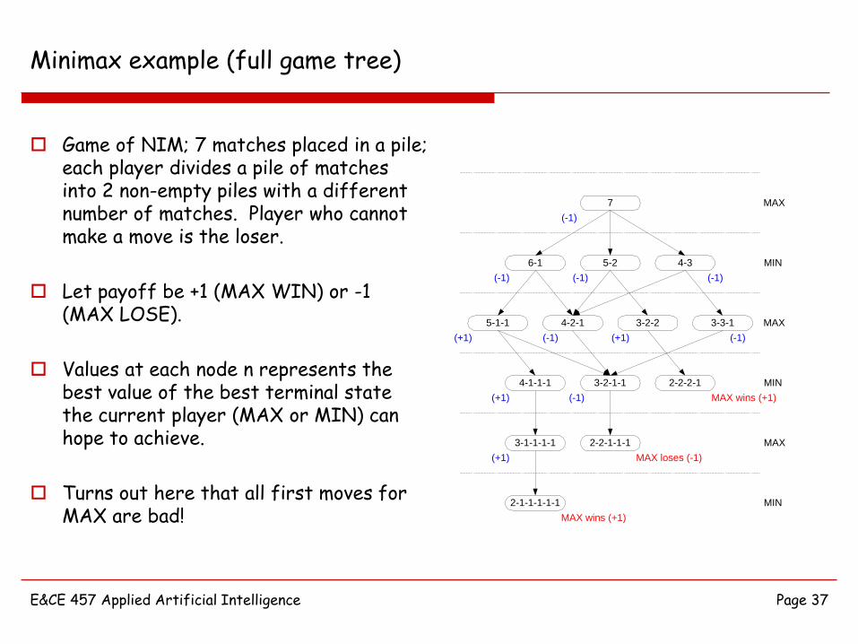
Game of NIM; 7 matches placed in a pile; each player divides a pile of matches into 2 non-empty piles with a different number of matches. Player who cannot make a move is the loser.
Let payoff be +1 (MAX WIN) or -1 (MAX LOSE).
Values at each node n represents the best value of the best terminal state the current player (MAX or MIN) can hope to achieve.
Turns out here that all first moves for MAX are bad!
5-1-1 4-2-1 3-2-2 3-3-1
6-1 5-2 4-3
7
4-1-1-1 3-2-1-1 2-2-2-1
3-1-1-1-1 2-2-1-1-1
2-1-1-1-1-1
MAX
MIN
MAX
MAX
MIN
MIN
MAX wins (+1)
MAX loses (-1)
MAX wins (+1)
(+1)
(+1) (-1)
(+1) (-1) (+1) (-1)
(-1) (-1) (-1)
(-1)

E&CE 457 Applied Artificial Intelligence Page 38
Minimax example (partial game tree)
Tree not deep enough for leaves to indicate win/lose; only “goodness” of game configuration (for MAX).
MAX would like to get to game configuration D, but MIN would not allow it.
MAX will choose to go to game configuration B.
Again, minimax assumes MIN plays perfectly using the same payoff function as MAX (i.e., plays optimally from the same point of view as MAX).
D F G J
A B C
SMAX
MIN
MAX
(100)
(5)
E H I
(3) (-1) (6) (5) (2) (9)
(-1) (5) (2)
E&CE 457 Applied Artificial Intelligence Page 39
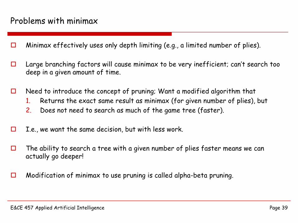
Problems with minimax
Minimax effectively uses only depth limiting (e.g., a limited number of plies).
Large branching factors will cause minimax to be very inefficient; can’t search too deep in a given amount of time.
Need to introduce the concept of pruning; Want a modified algorithm that
1. Returns the exact same result as minimax (for given number of plies), but
2. Does not need to search as much of the game tree (faster).
I.e., we want the same decision, but with less work.
The ability to search a tree with a given number of plies faster means we can actually go deeper!
Modification of minimax to use pruning is called alpha-beta pruning.

E&CE 457 Applied Artificial Intelligence Page 40
Pruning illustrated
A
E
F
D
C
B
MAX
MAX
MIN
1
4 8
payoff = 8
2
payoff <= 8
payoff >= 4
3
G
9
payoff >= 9
4
5
cutoff!
6
payoff >= 8
H
I
J
-2 7
payoff >= -2
E
2
8
payoff = 2
9
payoff <= 2
10
cutoff!
Prune at F after exploring G; F has payoff >= 9 (MAX); there exists a MIN ancestor with payoff <= 8; hence, MIN would prevent us from ever getting to F.
Prune at H after exploring I; H has payoff <= 2 (MIN); there exists a MAX ancestor with payoff >= 8; hence, MAX would prevent us from ever getting to H.
NumberedBoxes showSalient decisions

E&CE 457 Applied Artificial Intelligence Page 41
Alpha-beta pruning
The algorithm maintains two values and .
Both computed using payoffs propagated up the tree.
The represents the minimum score that the maximizing player is assured of at any point during the search.
The represents the maximum score that the minimizing player is assured of at any point during the search.
As the search of the game tree progresses the “window” of values decreases.
Fewer possible values for and .
Whenever becomes less than or equal to ( ≤ )
Current game configuration cannot be the result of the best play by both players and does not need to be explored further.
More later …

E&CE 457 Applied Artificial Intelligence Page 42
Alpha-beta pruning
Pseudo-code; called as evaluate(root,-infinity,+infinity)
evaluate (node, alpha, beta)
if node is a LEAF
return the PAYOFF value of node
if node is a MIN node
beta = +inf
for each child of node
beta = min (beta, evaluate (child, alpha, beta))
if beta <= alpha break
return beta
if node is a MAX node
alpha = -inf
for each child of node
alpha = max (alpha, evaluate (child, alpha, beta))
if beta <= alpha break
return alpha
E&CE 457 Applied Artificial Intelligence Page 43
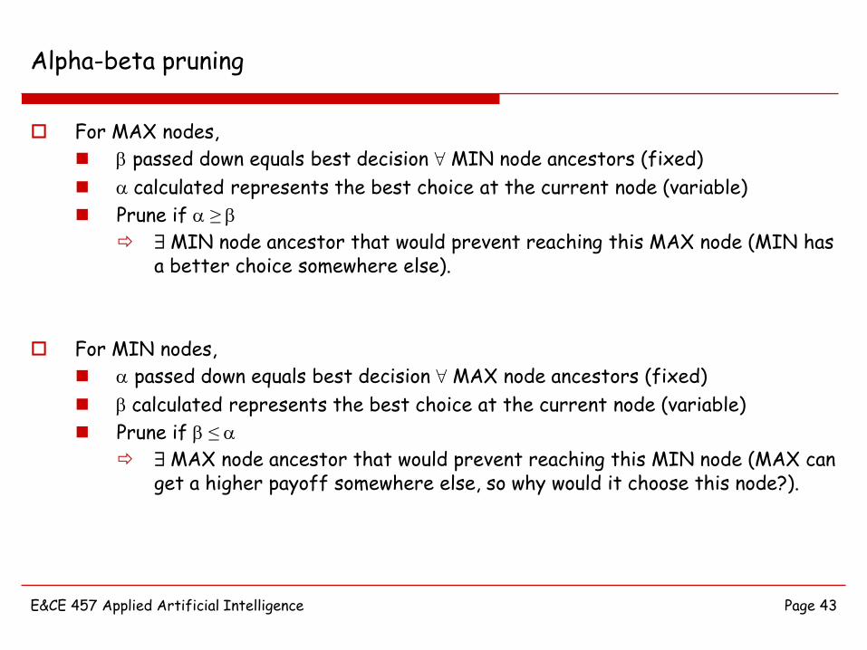
Alpha-beta pruning
For MAX nodes,
passed down equals best decision 8 MIN node ancestors (fixed)
calculated represents the best choice at the current node (variable)
Prune if ≥
9 MIN node ancestor that would prevent reaching this MAX node (MIN has a better choice somewhere else).
For MIN nodes,
passed down equals best decision 8 MAX node ancestors (fixed)
calculated represents the best choice at the current node (variable)
Prune if ≤
9 MAX node ancestor that would prevent reaching this MIN node (MAX can get a higher payoff somewhere else, so why would it choose this node?).

E&CE 457 Applied Artificial Intelligence Page 44
Pruning illustrated with (alpha,beta) values
4 8 9 -2 2
A
ED
C
B
MAX
MAX
MIN
F
G
H
I
J E
(-inf,+inf)
->(4,+inf)
->(8,+inf)
(-inf,+inf)
->(-inf,8)
(-inf,+inf)
->(8,+inf)
->(-inf,8)
->(9,8)
-> CUTOFF
(8,+inf)
->(8,2)
-> CUTOFF
->(-inf,+inf)
->(-2,+inf)
-> (2,+inf)
E&CE 457 Applied Artificial Intelligence Page 45
Games of chance
Game of chance is anything with a random factor; e.g., dice, cards, etc.
Can extend the minimax method to handle games of chance.
This results in an expectiminimax tree.
In an expectiminimax tree, levels of max and min nodes are interleaved with "chance" nodes.
Rather than taking the max or min of the payoff values of their children, chance nodes take a weighted average (expected value) of their children.
Weights are the probability that the chance node is reached.
Each chance node gets an “expectiminimax value”.
E&CE 457 Applied Artificial Intelligence Page 46
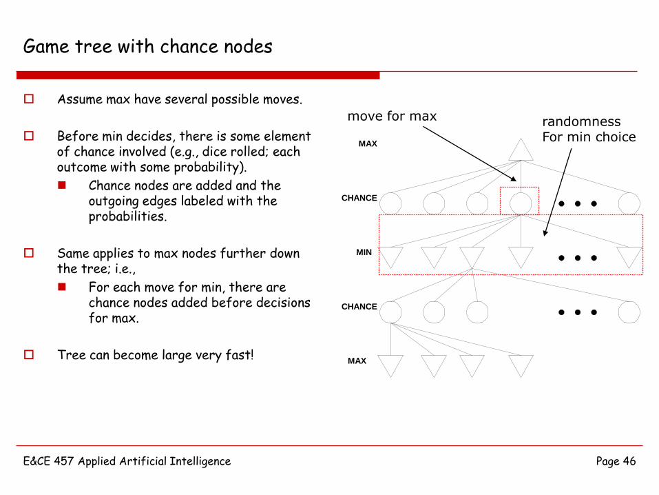
Game tree with chance nodes
Assume max have several possible moves.
Before min decides, there is some element of chance involved (e.g., dice rolled; each outcome with some probability).
Chance nodes are added and the outgoing edges labeled with the probabilities.
Same applies to max nodes further down the tree; i.e.,
For each move for min, there are chance nodes added before decisions for max.
Tree can become large very fast!
MAX
MIN
CHANCE
CHANCE
MAX
move for max randomnessFor min choice

E&CE 457 Applied Artificial Intelligence Page 47
Example of expectiminimax values
Example below shows calculation of weighted expected values at chance nodes.
Demonstrates potential problem when payoff function values are skewed;
Resulting values at chance nodes are an average (mean);
Large skewing in payoff values can cause MAX to make the wrong decision.
1 400 20 30
9/101/109/10 1/10
val = 9/10*1+1/10*400 = 40.9 val = 9/10*20+1/10*30 = 21
40.9


![I/O Management and Disk Scheduling - University of Waterloopami.uwaterloo.ca/~basir/ece354/chpt11cw-web.pdf · Disk Scheduling Policies[1] Seek time is the reason for differences](https://static.fdocuments.in/doc/165x107/5f598af00d0c8902e05aa43d/io-management-and-disk-scheduling-university-of-basirece354chpt11cw-webpdf.jpg)