
Informed Search A* Algorithm - Sharif
71
CE417: Introduction to Artificial Intelligence Sharif University of Technology Fall 2019 “Artificial Intelligence: A Modern Approach”, Chapter 3 Most slides have been adopted from Klein and Abdeel, CS188, UC Berkeley. Informed Search A* Algorithm Soleymani
Transcript of Informed Search A* Algorithm - Sharif

CE417: Introduction to Artificial IntelligenceSharif University of TechnologyFall 2019
“Artificial Intelligence: A Modern Approach”, Chapter 3Most slides have been adopted from Klein and Abdeel, CS188, UC Berkeley.
Informed SearchA* Algorithm
Soleymani

Outline} Heuristics} Greedy (best-first) search} A* search} Finding heuristics
2

Uninformed Search
3

Uniform Cost Search
} Strategy: expand lowest path cost
} The good: UCS is complete and optimal!
} The bad:} Explores options in every “direction”} No information about goal location Start Goal
…
c £ 3
c £ 2
c £ 1
4

UCS Example
5

Informed Search
6

Search Heuristics§ Aheuristicis:
§ Afunctionthatestimates howcloseastateistoagoal§ Designedforaparticularsearchproblem§ Examples:Manhattandistance,Euclideandistanceforpathing
10
5
11.2
7

Heuristic Function} Incorporating problem-specific knowledge in search
} Information more than problem definition} In order to come to an optimal solution as rapidly as possible
} ℎ 𝑛 : estimated cost of cheapest path from 𝑛 to a goal} Depends only on 𝑛 (not path from root to 𝑛)} If 𝑛 is a goal state then ℎ(𝑛)=0} ℎ(𝑛) ≥ 0
} Examples of heuristic functions include using a rule-of-thumb,an educated guess, or an intuitive judgment
8

Example: Heuristic Function
h(x)
9

Greedy Search
10

Greedy search} Priority queue based on ℎ(𝑛)
} e.g., ℎ'() 𝑛 =straight-line distance from n to Bucharest
} Greedy search expands the node that appears to beclosest to goal
Greedy
11

Example: Heuristic Function
h(x)
12

Romania with step costs in km
13

Greedy best-first search example
14

Greedy best-first search example
15

Greedy best-first search example
16

Greedy best-first search example
17

Greedy best-first search
} Expand the node that seems closest…
} What can go wrong?
18

Greedy best-first search
} Strategy: expand a node that you think is closest to agoal state} Heuristic: estimate of distance to nearest goal for each state
} A common case:} Best-first takes you straight to the (wrong) goal
} Worst-case: like a badly-guided DFS
…b
…b
19

Properties of greedy best-first search} Complete? No
} Similar to DFS, only graph search version is complete in finite spaces} Infinite loops, e.g., (Iasi to Fagaras) Iasi à Neamt à Iasi à Neamt
} Time} 𝑂(𝑏𝑚), but a good heuristic can give dramatic improvement
} Space} 𝑂(𝑏𝑚): keeps all nodes in memory
} Optimal? No
20

Greedy Search
21

A* Search
22

A* Search
UCS Greedy
A*
23

A* search} Idea: minimizing the total estimated solution cost} Evaluation function for priority 𝑓 𝑛 = 𝑔 𝑛 + ℎ(𝑛)
} 𝑔 𝑛 = cost so far to reach 𝑛} ℎ 𝑛 = estimated cost of the cheapest path from 𝑛 to goal} So, 𝑓 𝑛 = estimated total cost of path through 𝑛 to goal
24
start n… goal…
Actual cost 𝑔 𝑛 Estimated cost ℎ 𝑛
𝑓 𝑛 = 𝑔 𝑛 + ℎ(𝑛)

CombiningUCSandGreedy
} Uniform-cost orders by path cost, or backward cost g(n)} Greedy orders by goal proximity, or forward cost h(n)
} A* Search orders by the sum: f(n) = g(n) + h(n)
S a d
b
Gh=5
h=6
h=2
1
8
11
2
h=6 h=0
c
h=7
3
e h=11
Example:Teg Grenager
S
a
b
c
ed
dG
G
g=0h=6
g=1h=5
g=2h=6
g=3h=7
g=4h=2
g=6h=0
g=9h=1
g=10h=2
g=12h=0
25

WhenshouldA*terminate?
} Should we stop when we enqueue a goal?
} No: only stop when we dequeue a goal
S
B
A
G
2
3
2
2h=1
h=2
h=0h=3
26

IsA*Optimal?
• What went wrong?• Actual bad goal cost < estimated good goal cost• We need estimates to be less than actual costs!
A
GS
1 3h=6
h=0
5
h =7
27

Admissible Heuristics
28

Idea: Admissibility
Inadmissible(pessimistic)heuristicsbreakoptimalitybytrappinggoodplansonthefrontier
Admissible(optimistic)heuristicsslowdownbadplansbutneveroutweightruecosts
29

Admissible Heuristics
} A heuristic h is admissible (optimistic) if:
where is the true cost to a nearest goal
} Examples:
} Coming up with admissible heuristics is most of what’sinvolved in using A* in practice.
15
30

Optimality of A* Tree Search
31

OptimalityofA*TreeSearch
Assume:} A is an optimal goal node} B is a suboptimal goal node} h is admissible
Claim:
} A will exit the frontier before B
…
32

OptimalityofA*TreeSearch:Blocking
Proof:} Imagine B is on the frontier} Some ancestor n of A is on the
frontier, too (maybe A!)} Claim: n will be expanded before B
1. f(n) is less or equal to f(A)
Definitionoff-costAdmissibilityofh
…
h=0atagoal
𝑓 𝑛 ≤ 𝑔 𝑛 + ℎ∗(𝑛)𝑔 𝐴 = 𝑔 𝑛 + ℎ∗(𝑛)
33

OptimalityofA*TreeSearch:Blocking
Proof:} Imagine B is on the frontier} Some ancestor n of A is on the
frontier, too (maybe A!)} Claim: n will be expanded before B
1. f(n) is less or equal to f(A)2. f(A) is less than f(B)
Bissuboptimalh=0atagoal
…
34

OptimalityofA*TreeSearch:Blocking
Proof:} Imagine B is on the frontier} Some ancestor n of A is on the
frontier, too (maybe A!)} Claim: n will be expanded before B
1. f(n) is less or equal to f(A)2. f(A) is less than f(B)3. n expands before B
} All ancestors of A expand before B} A expands before B} A* search is optimal
…
35

A* search
36
} Combines advantages of uniform-cost and greedysearches
} A* can be complete and optimal when ℎ(𝑛) has someproperties

A* search: example
37

A* search: example
38

A* search: example
39

A* search: example
40

A* search: example
41

A* search: example
42

Graph Search
43
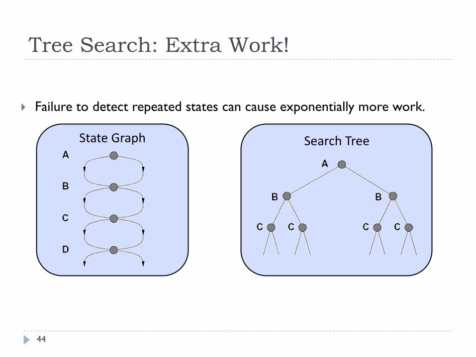
} Failure to detect repeated states can cause exponentially more work.
SearchTreeStateGraph
Tree Search: Extra Work!
44

GraphSearch} In BFS, for example, we shouldn’t bother expanding the circled nodes (why?)
S
a
b
d p
a
c
e
p
h
f
r
q
q c G
a
qe
p
h
f
r
q
q c G
a
45

Recall: Graph Search} Idea: never expand a state twice
} How to implement:
} Tree search + set of expanded states (“closed set”)
} Expand the search tree node-by-node, but…
} Before expanding a node, check to make sure its state has never been expanded before
} If not new, skip it, if new add to closed set
} Important: store the closed set as a set, not a list
} Can graph search wreck completeness? Why/why not?
} How about optimality?
46

Optimality of A* Graph Search
47

A*GraphSearchGoneWrong?
S
A
B
C
G
1
1
1
23
h=2
h=1
h=4
h=1
h=0
S(0+2)
A(1+4) B(1+1)
C(2+1)
G(5+0)
C(3+1)
G(6+0)
Statespacegraph Searchtree
48

Conditions for optimality of A*
} Admissibility: ℎ(𝑛) be a lower bound on the cost to reach goal} Condition for optimality of TREE-SEARCH version of A*
} Consistency (monotonicity): ℎ 𝑛 ≤ 𝑐 𝑛, 𝑎, 𝑛8 + ℎ 𝑛8} Condition for optimality of GRAPH-SEARCH version of A*
49
Consistent heuristics
50
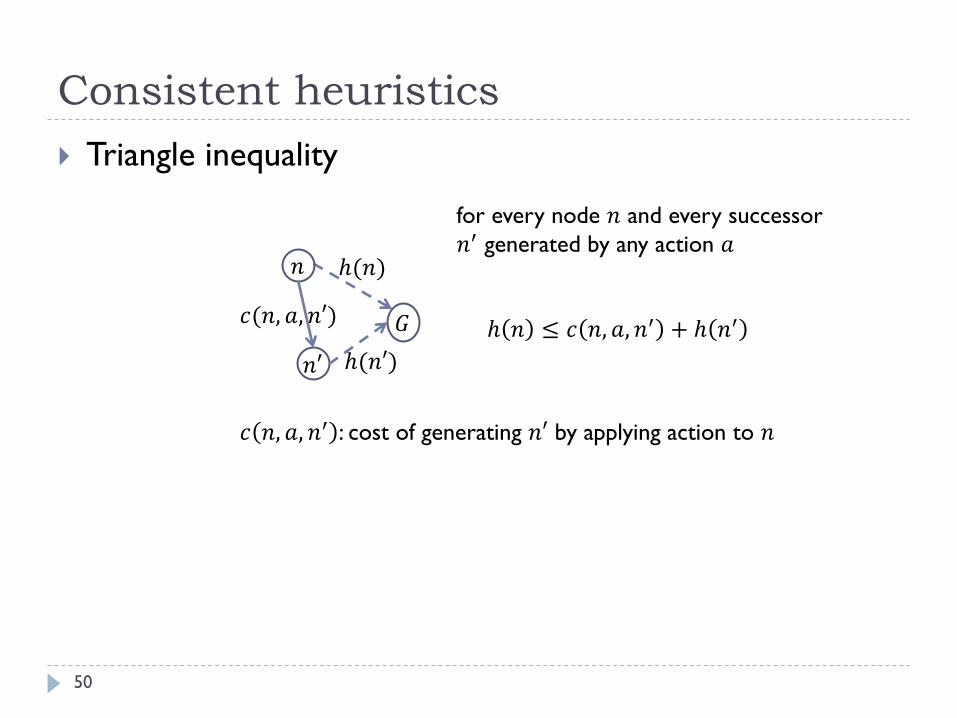
} Triangle inequality
𝑛
𝑛′
𝐺ℎ(𝑛′)
ℎ(𝑛)
𝑐(𝑛, 𝑎, 𝑛′)
𝑐 𝑛, 𝑎, 𝑛8 : cost of generating 𝑛′ by applying action to 𝑛
for every node 𝑛 and every successor𝑛8 generated by any action 𝑎
ℎ 𝑛 ≤ 𝑐 𝑛, 𝑎, 𝑛8 + ℎ 𝑛8

ConsistencyofHeuristics} Main idea: estimated heuristic costs ≤ actual costs
} Admissibility: heuristic cost ≤ actual cost to goal
h(A) ≤ actual cost from A to G
} Consistency: heuristic “arc” cost ≤ actual cost for each arc
h(A) – h(C) ≤ cost(A to C)
} Consequences of consistency:} The f value along a path never decreases
h(A) ≤ cost(A to C) + h(C)
} A* graph search is optimal
3
A
C
G
h=4 h=11
h=2
51

Admissible but not consistent: Example
52
} 𝑓 (for admissible heuristic) may decrease along a path} Is there any way to make ℎ consistent?
𝑛
𝑛′
𝑐(𝑛, 𝑎, 𝑛’) = 1ℎ(𝑛) = 9ℎ(𝑛’) = 6⟹ ℎ 𝑛 ≰ ℎ 𝑛’ + 𝑐(𝑛, 𝑎, 𝑛’)
1
𝑔 𝑛 = 5ℎ 𝑛 = 9𝑓(𝑛) = 14
𝑔 𝑛′ = 6ℎ 𝑛8 = 6𝑓(𝑛′) = 12G
10
10
ℎD 𝑛′ = max(ℎ 𝑛8 , ℎD 𝑛 − 𝑐(𝑛, 𝑎, 𝑛′))

Consistency implies admissibility
53
} Consistency ⇒Admissblity} All consistent heuristic functions are admissible} Nonetheless, most admissible heuristics are also consistent
ℎ 𝑛J ≤ 𝑐 𝑛J, 𝑎J, 𝑛K + ℎ(𝑛K)≤ 𝑐 𝑛J, 𝑎J, 𝑛K + 𝑐 𝑛K, 𝑎K, 𝑛L + ℎ(𝑛L)
…≤ ∑ 𝑐 𝑛N, 𝑎N, 𝑛NOJP
NQJ + ℎ(G)
𝑛J 𝑛K 𝑛L 𝑛P 𝐺…𝑐(𝑛J, 𝑎J, 𝑛K) 𝑐(𝑛P, 𝑎P, 𝐺)𝑐(𝑛K, 𝑎K, 𝑛L)
0 ⇒ ℎ 𝑛J ≤ cost of (every) path from 𝑛J to goal≤ cost of optimal path from 𝑛J to goal

Optimality} Tree search:
} A* is optimal if heuristic is admissible} UCS is a special case (h = 0)
} Graph search:} A* optimal if heuristic is consistent} UCS optimal (h = 0 is consistent)
} Consistency implies admissibility
} In general, most natural admissible heuristics tend to beconsistent, especially if from relaxed problems
54

OptimalityofA*GraphSearch} Sketch: consider what A* does with a consistent heuristic:
} Fact 1: In graph search, A* expands nodes in increasing total f value (f-contours)
} Fact 2: For every state s, nodes that reach s optimally are expanded before nodesthat reach s suboptimally
} Result: A* graph search is optimal…
f£ 3
f£ 2
f£ 1
55

Optimality of A* (consistent heuristics)Theorem: If ℎ(𝑛) is consistent, A* using GRAPH-SEARCH isoptimal
Lemma1: if ℎ(𝑛) is consistent then 𝑓(𝑛) values are non-decreasing along any path
Proof: Let 𝑛′ be a successor of 𝑛
I. 𝑓(𝑛′) = 𝑔(𝑛′) + ℎ(𝑛′)II. 𝑔(𝑛′) = 𝑔(𝑛) + 𝑐(𝑛, 𝑎, 𝑛′)III. 𝐼, 𝐼𝐼 ⇒ 𝑓 𝑛8 = 𝑔 𝑛 + 𝑐 𝑛, 𝑎, 𝑛8 + ℎ 𝑛8
IV. ℎ 𝑛 isconsistent ⇒ ℎ 𝑛 ≤ 𝑐 𝑛, 𝑎, 𝑛8 + ℎ 𝑛8 V. 𝐼𝐼𝐼, 𝐼𝑉 ⇒ 𝑓(𝑛′) ≥ 𝑔(𝑛) + ℎ(𝑛) = 𝑓(𝑛)
56

Optimality of A* (consistent heuristics)Lemma 2: For every state 𝑛, nodes that reach 𝑛 optimally areexpanded before nodes that reach 𝑛 sub-optimally
Proof by contradiction:Assume that 𝑛 has been selected for expansion. Another frontier node 𝑛8must exist on the optimal path from initial node to 𝑛 (using graph separationproperty). Moreover, based on Lemma 1, 𝑓 𝑛8 ≤ 𝑓 𝑛 and thus𝑛8wouldhave been selected first.
Lemma 1 & 2⇒ The sequence of nodes expanded by A* (using GRAPH-SEARCH) is in non-decreasing order of 𝑓(𝑛)
Since ℎ = 0 for goal nodes, the first selected goal node for expansion is anoptimal solution (𝑓 is the true cost for goal nodes)
57

Admissible vs. consistent (tree vs. graph search)
58
} Consistent heuristic: When selecting a node for expansion, thepath with the lowest cost to that node has been found
} When an admissible heuristic is not consistent, a node willneed repeated expansion, every time a new best (so-far) costis achieved for it.

Contours in the state space} A* (using GRAPH-SEARCH) expands nodes in order of
increasing 𝑓 value} Gradually adds "f-contours" of nodes
} Contour 𝑖 has all nodes with 𝑓 = 𝑓N where𝑓N < 𝑓N+1
A* expands all nodes with f(n) < C*A* expands some nodes with f(n) = C* (nodes on the goal contour)A* expands no nodes with f(n) > C*⟹pruning
59
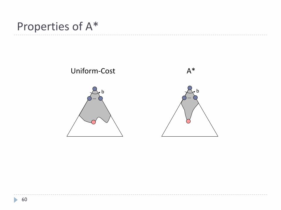
PropertiesofA*
…b
…b
Uniform-Cost A*
60

A* Example
61

Example
62
UCS Greedy A*

UCSvs A*Contours
} Uniform-cost (A* using ℎ(𝑛)=0) expandsequally in all “directions”
} A* expands mainly toward the goal, butdoes hedge its bets to ensure optimality} More accurate heuristics stretched toward the goal
(more narrowly focused around the optimal path)
Start Goal
Start Goal
States are points in 2-D Euclidean space.g(n)=distance from starth(n)=estimate of distance from goal
63

Comparison
GreedyUniformCost A*
64

Properties of A*} Complete?
} Yes if nodes with 𝑓 ≤ 𝑓 𝐺 = 𝐶∗ are finite} Step cost≥ 𝜀 > 0 and 𝑏 is finite
} Time?} Exponential
} But, with a smaller branching factor
¨ 𝑏d∗ed or when equal step costs 𝑏f×h∗ihh∗
} Polynomial when |ℎ(𝑥) − ℎ∗(𝑥)| = 𝑂(𝑙𝑜𝑔ℎ∗(𝑥))} However,A* is optimally efficient for any given consistent heuristic
} No optimal algorithm of this type is guaranteed to expand fewer nodes than A* (exceptto node with 𝑓 = 𝐶∗)
} Space?} Keeps all leaf and/or explored nodes in memory
} Optimal?} Yes (expanding node in non-decreasing order of 𝑓)
65

Robot navigation example
66
} Initial state? Red cell
} States? Cells on rectangular grid (except to obstacle)
} Actions? Move to one of 8 neighbors (if it is not obstacle)
} Goal test? Green cell
} Path cost? Action cost is the Euclidean length of movement

A* vs. UCS: Robot navigation example
67
} Heuristic: Euclidean distance to goal
} Expanded nodes: filled circles in red & green} Color indicating 𝑔 value (red: lower, green: higher)
} Frontier: empty nodes with blue boundary
} Nodes falling inside the obstacle are discarded
Adopted from: http://en.wikipedia.org/wiki/Talk%3AA*_search_algorithm

Robot navigation: Admissible heuristic
68
} Is Manhattan 𝑑o 𝑥, 𝑦 = 𝑥J − 𝑦J + 𝑥K − 𝑦K distancean admissible heuristic for previous example?

A*: inadmissible heuristic
69
ℎ = ℎ_𝑆𝐿𝐷ℎ = 5 ∗ ℎ_𝑆𝐿𝐷
Adopted from: http://en.wikipedia.org/wiki/Talk%3AA*_search_algorithm

A*: Summary
70

A*: Summary} A* uses both backward costs and (estimates of) forward
costs
} A* is optimal with admissible / consistent heuristics
} Heuristic design is key: often use relaxed problems
71


![Meelad Sharif [Urdu]](https://static.fdocuments.in/doc/165x107/577cb0ae1a28aba7118b45c7/meelad-sharif-urdu.jpg)


