THE UNIVERSITY OF CHICAGOA SEARCH FOR THE EXTRAGALACTIC MAGNETIC FIELD VIA ITSINFLUENCE ON THE GAMMA-RAY SIGNALS FROM BLAZARS

A DISSERTATION SUBMITTED TOTHE FACULTY OF THE DIVISION OF THE PHYSICAL SCIENCESIN CANDIDACY FOR THE DEGREE OFDOCTOR OF PHILOSOPHYDEPARTMENT OF PHYSICSBYTHOMAS RAYMOND WEISGARBER

CHICAGO, ILLINOISJUNE 2012

All rights reserved

INFORMATION TO ALL USERSThe quality of this reproduction is dependent on the quality of the copy submitted.

In the unlikely event that the author did not send a complete manuscriptand there are missing pages, these will be noted. Also, if material had to be removed,

a note will indicate the deletion.

All rights reserved. This edition of the work is protected againstunauthorized copying under Title 17, United States Code.

ProQuest LLC.789 East Eisenhower Parkway

P.O. Box 1346Ann Arbor, MI 48106 - 1346

UMI 3513560Copyright 2012 by ProQuest LLC.

UMI Number: 3513560

Copyright © 2012 by Thomas Raymond WeisgarberAll rights reserved

You bore me through a fog of years,And now I walk, for I have runA journey half omplete, begunBy you, whi h love of wisdom steers.

TABLE OF CONTENTSLIST OF FIGURES . . . . . . . . . . . . . . . . . . . . . . . . . . . . . . . . . . . . viiLIST OF TABLES . . . . . . . . . . . . . . . . . . . . . . . . . . . . . . . . . . . . . ixACKNOWLEDGMENTS . . . . . . . . . . . . . . . . . . . . . . . . . . . . . . . . . xABSTRACT . . . . . . . . . . . . . . . . . . . . . . . . . . . . . . . . . . . . . . . . xiiiCHAPTER1 EXTRAGALACTIC MAGNETIC FIELDS . . . . . . . . . . . . . . . . . . . . . . 11.1 EGMF Formation . . . . . . . . . . . . . . . . . . . . . . . . . . . . . . . . . 31.2 Evolution of the EGMF . . . . . . . . . . . . . . . . . . . . . . . . . . . . . 41.3 Limits on the EGMF . . . . . . . . . . . . . . . . . . . . . . . . . . . . . . . 51.4 Measuring the EGMF . . . . . . . . . . . . . . . . . . . . . . . . . . . . . . 72 EXTRAGALACTIC BACKGROUNDS AND INTERACTIONS . . . . . . . . . . 92.1 Isotropi Ba kgrounds . . . . . . . . . . . . . . . . . . . . . . . . . . . . . . 92.2 Pair Produ tion . . . . . . . . . . . . . . . . . . . . . . . . . . . . . . . . . . 122.2.1 Kinemati s . . . . . . . . . . . . . . . . . . . . . . . . . . . . . . . . 122.2.2 Produ t Angles and Energies . . . . . . . . . . . . . . . . . . . . . . 152.3 Inverse Compton S attering . . . . . . . . . . . . . . . . . . . . . . . . . . . 172.3.1 Kinemati s . . . . . . . . . . . . . . . . . . . . . . . . . . . . . . . . 182.3.2 Produ t Angles and Energies . . . . . . . . . . . . . . . . . . . . . . 212.4 The Mean Free Path for Intera tions . . . . . . . . . . . . . . . . . . . . . . 232.4.1 Pair Produ tion . . . . . . . . . . . . . . . . . . . . . . . . . . . . . . 232.4.2 Inverse Compton S attering . . . . . . . . . . . . . . . . . . . . . . . 242.4.3 Inuen e of the Cas ades . . . . . . . . . . . . . . . . . . . . . . . . . 262.4.4 Redshift Generalizations . . . . . . . . . . . . . . . . . . . . . . . . . 272.5 The Lorentz For e . . . . . . . . . . . . . . . . . . . . . . . . . . . . . . . . 282.6 Other Pro esses . . . . . . . . . . . . . . . . . . . . . . . . . . . . . . . . . . 293 GAMMA-RAY SOURCES AND DETECTION TECHNIQUES . . . . . . . . . . 323.1 Blazars . . . . . . . . . . . . . . . . . . . . . . . . . . . . . . . . . . . . . . . 323.2 The Fermi Instrument . . . . . . . . . . . . . . . . . . . . . . . . . . . . . . 353.3 Imaging Atmospheri Cherenkov Teles opes . . . . . . . . . . . . . . . . . . 383.4 Other Dete tion Te hniques . . . . . . . . . . . . . . . . . . . . . . . . . . . 404 LIMITS ON THE EGMF FROM A SEMI-ANALYTIC MODEL . . . . . . . . . . 414.1 Cas ade Model . . . . . . . . . . . . . . . . . . . . . . . . . . . . . . . . . . 414.2 EGMF Predi tions and Limits . . . . . . . . . . . . . . . . . . . . . . . . . . 464.3 A ura y and Domain of Validity . . . . . . . . . . . . . . . . . . . . . . . . 52iv

5 MONTE CARLO SIMULATION . . . . . . . . . . . . . . . . . . . . . . . . . . . 545.1 Capabilities and A ura y . . . . . . . . . . . . . . . . . . . . . . . . . . . . 545.1.1 Modular Design . . . . . . . . . . . . . . . . . . . . . . . . . . . . . . 545.1.2 Parti le Kinemati s . . . . . . . . . . . . . . . . . . . . . . . . . . . . 555.1.3 Parti le Tra king . . . . . . . . . . . . . . . . . . . . . . . . . . . . . 655.1.4 Energy Losses . . . . . . . . . . . . . . . . . . . . . . . . . . . . . . . 705.1.5 Magneti Fields . . . . . . . . . . . . . . . . . . . . . . . . . . . . . . 725.1.6 Multigenerational Cas ades . . . . . . . . . . . . . . . . . . . . . . . 725.2 Analysis and Interpretation . . . . . . . . . . . . . . . . . . . . . . . . . . . 735.2.1 Geometry . . . . . . . . . . . . . . . . . . . . . . . . . . . . . . . . . 735.2.2 The Cas ade Flux . . . . . . . . . . . . . . . . . . . . . . . . . . . . . 755.3 Adequate Statisti s . . . . . . . . . . . . . . . . . . . . . . . . . . . . . . . . 785.3.1 The Transition Energy . . . . . . . . . . . . . . . . . . . . . . . . . . 785.3.2 The Transfer Fun tion . . . . . . . . . . . . . . . . . . . . . . . . . . 815.3.3 Overall A ura y . . . . . . . . . . . . . . . . . . . . . . . . . . . . . 835.4 General Predi tions . . . . . . . . . . . . . . . . . . . . . . . . . . . . . . . . 835.4.1 Spe tra . . . . . . . . . . . . . . . . . . . . . . . . . . . . . . . . . . 845.4.2 Energy-Dependent Morphology . . . . . . . . . . . . . . . . . . . . . 845.4.3 Time Proles . . . . . . . . . . . . . . . . . . . . . . . . . . . . . . . 906 THE SEARCH FOR BLAZAR HALOS IN THE EGMF CONTEXT . . . . . . . 926.1 Assumptions . . . . . . . . . . . . . . . . . . . . . . . . . . . . . . . . . . . . 926.1.1 The Time Prole . . . . . . . . . . . . . . . . . . . . . . . . . . . . . 936.1.2 Relativisti Beaming . . . . . . . . . . . . . . . . . . . . . . . . . . . 936.1.3 Simulation Limits . . . . . . . . . . . . . . . . . . . . . . . . . . . . . 946.1.4 The Intrinsi Spe trum . . . . . . . . . . . . . . . . . . . . . . . . . . 946.1.5 The EGMF Model . . . . . . . . . . . . . . . . . . . . . . . . . . . . 956.1.6 Properties of the Cas ade . . . . . . . . . . . . . . . . . . . . . . . . 956.2 Data Analysis . . . . . . . . . . . . . . . . . . . . . . . . . . . . . . . . . . . 966.2.1 Ground-Based Instruments . . . . . . . . . . . . . . . . . . . . . . . . 966.2.2 Fermi Data . . . . . . . . . . . . . . . . . . . . . . . . . . . . . . . . 976.2.3 Combining the Data . . . . . . . . . . . . . . . . . . . . . . . . . . . 996.3 Data Veri ation . . . . . . . . . . . . . . . . . . . . . . . . . . . . . . . . . 1006.3.1 Pro edure . . . . . . . . . . . . . . . . . . . . . . . . . . . . . . . . . 1016.3.2 Tests . . . . . . . . . . . . . . . . . . . . . . . . . . . . . . . . . . . . 1026.4 Halo Limits . . . . . . . . . . . . . . . . . . . . . . . . . . . . . . . . . . . . 1096.4.1 RGB J0710+591 . . . . . . . . . . . . . . . . . . . . . . . . . . . . . 1106.4.2 1ES 0229+200 . . . . . . . . . . . . . . . . . . . . . . . . . . . . . . . 1116.4.3 Combined Limit . . . . . . . . . . . . . . . . . . . . . . . . . . . . . . 1157 STRONG EXTRAGALACTIC MAGNETIC FIELDS . . . . . . . . . . . . . . . . 1177.1 Interpretation of the Results . . . . . . . . . . . . . . . . . . . . . . . . . . . 1177.2 Prospe ts for the Future . . . . . . . . . . . . . . . . . . . . . . . . . . . . . 121v

APPENDIXA EQUATIONS OF MOTION IN COMOVING COORDINATES . . . . . . . . . . 123A.1 Parti le Dynami s . . . . . . . . . . . . . . . . . . . . . . . . . . . . . . . . . 123A.2 Linear Motion . . . . . . . . . . . . . . . . . . . . . . . . . . . . . . . . . . . 125A.3 Ele tromagneti Fields . . . . . . . . . . . . . . . . . . . . . . . . . . . . . . 128B MEAN FREE PATH SAMPLING FOR CONTINUOUS ENERGY LOSSES . . . 130C GLOSSARY OF TLAS AND TMLAS . . . . . . . . . . . . . . . . . . . . . . . . 134REFERENCES . . . . . . . . . . . . . . . . . . . . . . . . . . . . . . . . . . . . . . . 135

vi

LIST OF FIGURES1.1 Existing limits on the EGMF strength and orrelation length. . . . . . . . . 62.1 Measurements and onstraints on the EBL at z = 0. . . . . . . . . . . . . . . 102.2 Re ent history of the CMB and EBL. . . . . . . . . . . . . . . . . . . . . . . 112.3 Kinemati s of the pair produ tion intera tion. . . . . . . . . . . . . . . . . . 132.4 Total ross se tion for pair produ tion. . . . . . . . . . . . . . . . . . . . . . 142.5 Pair produ tion dierential ross se tion as a fun tion of the ele tron emissionangle in the enter of momentum frame. . . . . . . . . . . . . . . . . . . . . 162.6 Kinemati s of the inverse Compton s attering intera tion. . . . . . . . . . . 182.7 Total ross se tion for inverse Compton s attering. . . . . . . . . . . . . . . 202.8 Dierential ross se tion for inverse Compton s attering intera tions. . . . . 212.9 The integrand of Equation 2.23 and the isotropi ba kground photon distri-bution. . . . . . . . . . . . . . . . . . . . . . . . . . . . . . . . . . . . . . . . 242.10 The integrand of Equation 2.24. . . . . . . . . . . . . . . . . . . . . . . . . . 252.11 The mean free path for pair produ tion and inverse Compton s attering. . . 262.12 Geometry relevant to the extragala ti as ades. . . . . . . . . . . . . . . . . 283.1 S hemati diagram of the Fermi LAT. . . . . . . . . . . . . . . . . . . . . . 353.2 Fermi LAT point-spread fun tion. . . . . . . . . . . . . . . . . . . . . . . . . 363.3 The stereo re onstru tion te hnique. . . . . . . . . . . . . . . . . . . . . . . 394.1 Example ts of the model's predi tions for the spe trum. . . . . . . . . . . . 454.2 Example t for B = 3 × 10−16 Gauss. . . . . . . . . . . . . . . . . . . . . . . 474.3 Maps of the χ2 value from a t to the RGB J0710+591 data, as a fun tion of uto energy and spe tral index. . . . . . . . . . . . . . . . . . . . . . . . . 494.4 Test-statisti urves from the intrinsi -spe trum s an. . . . . . . . . . . . . . 504.5 Limit on the EGMF as a fun tion of blazar lifetime. . . . . . . . . . . . . . . 525.1 Distribution of produ t ele tron and positron energies from gamma rays un-dergoing pair produ tion on a 30-meV monoenergeti ba kground. . . . . . . 565.2 Distribution of q for pair produ tion targets when the ba kground is monoen-ergeti at 30 meV. . . . . . . . . . . . . . . . . . . . . . . . . . . . . . . . . . 575.3 Distribution of target energies for pair produ tion on the EBL at a redshiftof z = 0.1. . . . . . . . . . . . . . . . . . . . . . . . . . . . . . . . . . . . . . 585.4 Distribution of intera tion lengths for pair produ tion on the EBL at a redshiftof z = 0.1. . . . . . . . . . . . . . . . . . . . . . . . . . . . . . . . . . . . . . 595.5 Distribution of produ t gamma-ray energies from inverse Compton s atteringas a fra tion of maximum possible energy. . . . . . . . . . . . . . . . . . . . 605.6 Distribution of x from inverse Compton s attering. . . . . . . . . . . . . . . 615.7 Distribution of target photon energies for inverse Compton s attering by 10-TeV ele trons at nearby redshift. . . . . . . . . . . . . . . . . . . . . . . . . 635.8 Distribution of 10-TeV ele trons' intera tion lengths for inverse Compton s at-tering. . . . . . . . . . . . . . . . . . . . . . . . . . . . . . . . . . . . . . . . 64vii

5.9 A ura y of total momentum onservation for both pair produ tion and in-verse Compton s attering. . . . . . . . . . . . . . . . . . . . . . . . . . . . . 655.10 A ura y of momentum onservation transverse to the dire tion of the pri-mary, for pair produ tion and inverse Compton s attering. . . . . . . . . . . 665.11 Redshift dependen e of the relative error on the momentum of ele trons andgamma rays inje ted at z = 1. . . . . . . . . . . . . . . . . . . . . . . . . . . 685.12 Comoving distan e as a fun tion of redshift for parti les in a onstant-dominated osmology. . . . . . . . . . . . . . . . . . . . . . . . . . . . . . . . . . . . . . 695.13 Time delay of ele trons with respe t to a gamma ray propagating from z = 1to z = 0. . . . . . . . . . . . . . . . . . . . . . . . . . . . . . . . . . . . . . . 705.14 Paths of 100-GeV ele trons in omoving oordinates. . . . . . . . . . . . . . 715.15 Distributions of se ondary gamma rays from 5,000 20-TeV primaries inje tedat z = 0.13. . . . . . . . . . . . . . . . . . . . . . . . . . . . . . . . . . . . . 735.16 Geometry relevant to the interpretation of the as ade. . . . . . . . . . . . . 745.17 Simulated sky map of the as ade gamma rays from a misaligned blazar. . . 765.18 Simulated spe trum of the as ade emission from a misaligned blazar. . . . . 775.19 Errors on the ele tron energy distributions for various transition energies. . . 805.20 Spe tra for a sour e at z = 0.13 with an intrinsi spe tral index of 1.5. . . . 855.21 Extended halo emission for two eld strengths. . . . . . . . . . . . . . . . . . 865.22 Extended halo emission for B = 10−16 Gauss at four dierent energies. . . . 875.23 Ratio of the 68% ontainment radius of gamma rays in the halo with respe tto that of the Fermi LAT. . . . . . . . . . . . . . . . . . . . . . . . . . . . . 885.24 Fra tion of gamma rays in the as ade. . . . . . . . . . . . . . . . . . . . . . 895.25 Chara teristi time proles of the as ade. . . . . . . . . . . . . . . . . . . . 916.1 Summary of the results of Test 1 from Table 6.3.1. . . . . . . . . . . . . . . . 1036.2 Likelihood statisti maps for Test 2 from Table 6.3.1. . . . . . . . . . . . . . 1046.3 Summary of the results of Test 2 from Table 6.3.1. . . . . . . . . . . . . . . . 1066.4 Summary of the results of Test 3 from Table 6.3.1. . . . . . . . . . . . . . . . 1076.5 Summary of the results of Test 4 from Table 6.3.1. . . . . . . . . . . . . . . . 1086.6 Total observed gamma-ray spe trum of RGB J0710+591. . . . . . . . . . . . 1096.7 Likelihood statisti maps from the analysis of RGB J0710+591. . . . . . . . 1116.8 Summary of the results from the analysis of RGB J0710+591. . . . . . . . . 1126.9 Total observed gamma-ray spe trum of 1ES 0229+200. . . . . . . . . . . . . 1136.10 Summary of the results from the analysis of 1ES 0229+200. . . . . . . . . . 1146.11 The ombined likelihood statisti urve from the analysis of RGB J0710+591and 1ES 0229+200. . . . . . . . . . . . . . . . . . . . . . . . . . . . . . . . . 115viii

LIST OF TABLES4.1 Sele t onden e limits from a χ2(1) distribution. . . . . . . . . . . . . . . . 505.1 Pro essing times with and without a transition energy of 300 GeV for as adesof various energies. . . . . . . . . . . . . . . . . . . . . . . . . . . . . . . . . 785.2 CMB and EBL densities, along with ǫmax as dened by Equation 5.13, atspe i redshifts. . . . . . . . . . . . . . . . . . . . . . . . . . . . . . . . . . 816.1 Results from Fermi data analyses with the full Gala ti diuse and ut Gala -ti diuse models for the blazar RGB J0710+591. . . . . . . . . . . . . . . . 996.2 Parameters from one predetermined and three randomly sele ted models forthe intrinsi spe trum of RGB J0710+591. . . . . . . . . . . . . . . . . . . . 102C.1 List of TLAs and TMLAs. . . . . . . . . . . . . . . . . . . . . . . . . . . . . 134

ix

ACKNOWLEDGMENTSFor my growth as a s ientist, for my emotional stability, and for my ontinued fas inationwith the laws by whi h this universe is governed, I am indebted to innumerable individuals.I regret that, in the interests of e onomy, I annot name them all in the spa e of these A -knowledgments. Nevertheless, the inuen e of those olleagues, friends, and family memberswho have guided and ontinue to guide me remains present in my thoughts.For my intelle tual development as a s ientist, I am most grateful to my advisor, S ottWakely. Of all the things he taught me, the most important is to fo us on the simpleexplanations without whi h a truly deep understanding of the physi s an never be ultivated.S ott was there when I needed him and absent when I didn't. Hao Huan, my friend and olleague, also helped me via many insightful dis ussions that lead to new approa hes andnew ideas. My intera tions with Hao made me realize how valuable it is to have someonewith whom I an toss around new ideas, no matter how razy they sound. Steph Wissel,Brian Humensky, and Luis Reyes helped me immensely in nding my pla e at the Universityof Chi ago and in embarking and ontinuing on the path of astroparti le physi s resear h. Iam also parti ularly grateful to the late Simon Swordy, whose unique perspe tive onvin edme to ome to Chi ago in the rst pla e, and who taught me that it is not only progress,but progress plus initial onditions, that has made the world what it is today.In addition to my advisor, S ott Wakely, I would like to thank the members of my thesis ommittee, Dietri h Müller, Carlos Wagner, and David S huster, for taking time out of theirbusy s hedules to meet with me and dis uss my resear h. I would parti ularly like to thankDietri h Müller for frequently stopping by my o e with interesting questions.My membership in the Very Energeti Radiation Imaging Teles ope Array System (VER-ITAS) ollaboration has inspired in me a sense of teamwork in addition to a fondness forinordinately ontrived a ronyms. Tim Arlen and Vladimir Vassiliev deserve my espe ialthanks for the hospitality they showed me on my two visits to UCLA, during whi h we testedmu h of the Monte Carlo simulation used in this work and dis ussed the interpretation ofits results. Other members of VERITAS to whom I am grateful in lude, in no parti ularorder, Ester Aliu, Taylor Aune, Reshmi Mukherjee, Nahee Park, Je Grube, Jamie Holder,Vikram Dwarkadas, and Daniel Gall.Someone on e told me that graduate s hool is the best time of your life. That may bex

so. Like any other aspe t of life, however, it follows a pattern of highs and lows. The manyfriends that I have made while a graduate student have helped me through these tryingtimes. I am grateful to Mi hael Herman and Austin Carter for going along with my razyideas and over-fondness for games, to Tomm S aife for spelling his name with more m'sthan mine, and to Phil Killewald, the sour e of all sar asm, for being patient enough towork on problems in quantum eld theory with me. Thanks are due also to Wes Ket humand Dave M Cowan for keeping me in ne spirits, to Chris Williams for keeping me up todate on news and politi s and trying to graduate before me, and to the members of Physi sHouse, Ellen Martinsek, Joey Paulsen, Gabe Lee, and Emily Conover, for being interestingand entertaining roommates. My heartiest thanks go to Andreas Obermeier, who taught methat sometimes it's okay not to eat lun h at your desk, even though I'm doing exa tly that asI write this, and to Peggy Eppink, who is one of the few people I know who is willing to follownearly any spontaneous suggestion at least on e. I ould not have hoped1 for a better pairof friends with whom to ride in a onvertible in winter or be o in our ba k-of-the-envelope al ulations by more than fteen orders of magnitude.I also owe spe ial thanks to Sandy Heinz. When I rst ame to Chi ago, it was a hallenging time for me personally, and I felt overwhelmed settling into a new routine.Sandy set me up in the visitors' o e, helped me gure out how to get around Chi ago, andmade me feel right at home. As someone who knows everything about how the universityworks, Sandy has been both essential and a good friend.A few individuals deserving of thanks defy lassi ation and so I in lude them here. Ithank Jim Beatty for advising me to apply to the University of Chi ago, the members of theAstroparti le Journal Club for hoosing interesting topi s for review, Linn Van Woerkom,Enam Chowdhury, and Patri k Randerson for en ouraging me during my undergraduateyears and making physi s fun, Randy Bal h for alling every few months to remind me thatI haven't graduated yet, Kit and Possamer for their unswerving devotion, and the Hausenfor maintaining the logi al operation of physi s in the observable universe.I owe eternal thanks to Nahee Park for her patien e during these past few months, andapologies for assuming she was a professor when we rst met. Thanks to Nahee, the pastyear or so has been one of the most ex iting and happiest times of my life. She possesses1. In any reasonable sense. xi

an aggravating but honest frankness about my ability to dis uss physi s. While now I maynot be mat hing her in rank, at least I will have attained the same edu ational level. It ismy sin ere hope that for us the friendship of the past and the ex itement of the present maya tualize all of the promise of the future.Most importantly, I thank my family for their love and devotion throughout my life. Myparents taught me to be imaginative and dis iplined. My brother Mi hael, through longsuering, taught me ompassion and empathy. Grandma Ali e taught me to be urious andGrandma Dawn taught me to be self-reliant. All of them taught me love. Together, theirsupport has been the garden within whi h the seeds of my knowledge took root and grew.What they have done for me I hope also I have done for them.

xii

ABSTRACTObservations of the galaxies, lusters, and laments of the large-s ale stru ture (LSS) of theuniverse reveal that these obje ts possess magneti elds exhibiting ompli ated stru turewith strengths on the order of a mi roGauss. Re ent observations have also begun to shedlight on the extragala ti magneti eld (EGMF), whi h is believed to exist in the voidsthat likely omprise the majority of the LSS. Su h a eld ould have been generated primor-dially, for instan e during phase transitions in the early universe. In this ase, its dete tionand hara terization ould reveal information about onditions in the early universe. Aprimordially generated eld is also physi ally ompelling be ause many models of magneti eld formation in galaxies require an initial seed eld, a role that an be readily lled byan EGMF existing prior to galaxy formation. Alternatively, astrophysi al me hanisms havebeen proposed to generate the EGMF via bulk outows of magnetized plasma from a tiveand starburst galaxies. In this ase, the dete tion of an EGMF would provide eviden e forthe unexpe ted e ien y in the transport of magneti energy into the voids.Over the past few de ades, the development of ground-based gamma-ray astronomy hasopened many new opportunities to study the universe at high energies. One su h opportunityinvolves a re ently developed te hnique exploiting the observations of distant blazars tomeasure or onstrain the EGMF. Be ause of the osmologi al distan es that they must ross to propagate to Earth, very-high-energy gamma rays from blazars are attenuated bytheir intera tions with the extragala ti ba kground light and osmi mi rowave ba kgroundradiation. Due to this attenuation, an ele tromagneti as ade of ele trons, positrons, andgamma rays arises in extragala ti spa e. The dee tion of the ele trons and positrons bythe EGMF ultimately produ es two ee ts on the se ondary gamma rays in the as ades.These gamma rays are delayed in time with respe t to a primary gamma ray that travelsdire tly from the sour e to Earth, and they form an angular distribution, or halo, aroundwhat would otherwise appear as a pointlike blazar.In this work, I develop a new method for a urately quantifying the extended gamma-ray halo that arises due to the inuen e of the EGMF on the extragala ti as ades. Thismethod is sensitive to EGMF strengths between 3× 10−17 and 10−14 Gauss. I ompare thepredi tions from a Monte Carlo simulation to ombined data from ground-based imagingatmospheri Cherenkov teles opes and the Fermi Gamma-Ray Spa e Teles ope in an attemptxiii

to measure or onstrain the properties of the EGMF. Depending on ertain assumptionsabout the sour e lifetime, I interpret the absen e of any dete table gamma-ray halo aroundthe blazars RGB J0710+591 and 1ES 0229+200 as eviden e for an EGMF with a strengthgreater than 3 × 10−15 Gauss. This represents the strongest rm lower limit on the EGMFstrength at the present time.

xiv

CHAPTER 1EXTRAGALACTIC MAGNETIC FIELDSLarge-s ale magneti elds are ommon throughout the universe. Within our own Galaxy,numerous measurements have revealed a ri h stru ture of magneti elds via su h diversete hniques as the dete tion of polarized starlight, syn hrotron emission from populations ofrelativisti ele trons, Zeeman splitting of absorption lines, and the wavelength-dependentFaraday rotation of light from extragala ti sour es. These observations indi ate that theGala ti magneti eld strength is on the order of a few µGauss, with both large-s ale andrandom omponents (Be k, 2008).As might be expe ted, outside of the Galaxy, magneti elds tra e the matter distributionin the large-s ale stru ture (LSS) of the universe remarkably well. Galaxies in the LSS aregrouped into large regions known as lusters, whi h are onne ted by relatively thin regionsof galaxies known as laments. Surrounding the lusters and laments are the mostly emptyvoid regions that omprise the majority of the volume of the universe. Observations ofpolarized syn hrotron radiation from galaxies and lusters provide an in situ measurementof the magneti eld and have been used to demonstrate that magneti elds on the orderof 0.1 to 10 µGauss exist in nearly all galaxies and lusters (Widrow, 2002). Somewhatsurprisingly, the intra luster elds an be just as strong, if not stronger, than the gala ti elds. Magneti elds in the laments have also been measured in at least one instan e nearthe Coma luster (Kim et al., 1989; Kronberg et al., 2007). In general, the dete tion of theseelds rules out still higher eld strengths in the voids.In spite of the many measurements of magneti elds in galaxies and lusters, a positivedete tion of the extragala ti magneti eld (EGMF), presumed to exist in the voids, remainselusive. Theoreti al motivation for the existen e of this eld omes from a variety of sour es.The existen e of an EGMF during the epo h of galaxy formation ould provide the seed eldsne essary for many models of gala ti magneti eld formation (Grasso & Rubinstein, 2001).One possible sour e of the EGMF is from phase transitions in the early universe, during whi hthe misalignment between density and pressure gradients in the plasma an generate a eldvia the Biermann battery me hanism (Biermann, 1950). Alternative s enarios in whi h theEGMF is generated due to the bulk transport of magnetized plasma from the lobes of a tivegalaxies or other astrophysi al sour es have also been proposed (Kronberg, 1994; Kronberg1

et al., 2001).If it is generated through astrophysi al pro esses, the EGMF is expe ted to have a verysmall strength. To get a sense of what small means in this ontext, it is helpful to onsidera very simple ase in whi h the magneti eld of a galaxy is approximated by a dipole. Letus take the hara teristi size of the galaxy to be 10 kp and assume that the dipole eldat this distan e is 1 µGauss. If the galaxy is lo ated on the edge of a void whose enter is10 Mp away, then the distan e from the galaxy to the enter of the void is a fa tor of 103times larger than the size of the galaxy. Consequently, the dipole eld, whi h de reases withthe ube of the distan e from the dipole, will be redu ed by a fa tor of 109 to a magneti eld strength of 10−15 Gauss.However, the dipole approximation applied to gala ti elds is likely to be quite poor.Observationally, the eld strength in the galaxy does not fall with the ube of the distan e,but is relatively onstant throughout the gala ti plane. The onventional explanation forthese observations is that gala ti magneti elds are formed via magnetohydrodynami pro esses in the galaxy (Widrow, 2002). In the limit of large ondu tivity, magneti eldlines are frozen in to the plasma in the galaxy and an be stret hed and enhan ed by thebulk movement of the plasma due to the dierential rotation of the galaxy. The magneti eld outside the galaxy is then expe ted to be mu h weaker than the simple estimate suppliedby the dipole approximation.If the sour e of the EGMF is primordial instead of astrophysi al, then the problem of itsgeneration is moved from the present day to the early universe. In some sense this makesthe problem easier, sin e olle tive ee ts in the plasma of the early universe an generatethe eld. A magneti eld of any strength generated in the early universe an survive to thepresent day, provided that its orrelation length is su iently large to over ome magneti diusion.Faraday rotation and Zeeman splitting measurements of the light from distant quasarsrule out the existen e of an EGMF with a strength greater than the Gala ti eld. Whenthe ee ts of the Gala ti magneti eld are subtra ted from these measurements, upperlimits on the EGMF strength remain. However, until re ently, no lower limits on the EGMFstrength existed. In this work, I fo us on a newly developed method that enables a sear hfor the dominant omponent of the EGMF in the void regions of the LSS. The method relieson gamma-ray observations of blazars, a tive gala ti nu lei (AGN) with a jet oriented along2

or near the line of sight. Blazars that are dete ted at energies above 1 TeV an produ eele tromagneti as ades via intera tions with ba kground photons, and observations of these ondary gamma rays from these as ades an then be used to pla e limits on the strength ofthe EGMF. In some ases, it may be possible to measure the EGMF via these observations.Unless otherwise spe ied, throughout the rest of this work, I use the term EGMF todenote the dominant omponent of magneti elds in the voids, ignoring the elds in therest of the LSS. 1.1 EGMF FormationThe motivation for dete ting the EGMF is intri ately onne ted to its method of produ tionand its relationship to the elds dete ted in galaxies and lusters. If the EGMF is of primor-dial origin, it may have been produ ed during the ele troweak or quantum hromodynami phase transitions, during ination, or via exoti pro esses su h as the generation of primor-dial vorti ity by osmi strings (Grasso & Rubinstein, 2001). In general, these pro essesare invoked to generate ele tri elds and density u tuations ne essary for the operation ofthe Biermann battery or similar me hanisms. The measurement of a primordially generatedEGMF would provide insights into onditions in the early universe. Additionally, severalresear hers have suggested theoreti al me hanisms that ould amplify extragala ti seedelds, explaining the formation of the observed gala ti and luster elds, and a primordialEGMF ould provide these seed elds. One popular me hanism, the α-ω dynamo, relies onthe dierential rotation of galaxies to stret h and enhan e the eld lines. The dynamo oper-ates by stret hing poloidal omponents of the eld into toroidal omponents via dierentialrotation of matter in the galaxy, and also by onverting toroidal omponents into poloidal omponents via heli al disturban es in the ow of the plasma arrying the eld lines. Thesetwo ee ts lead to an overall enhan ement of the initial seed eld, possibly by many ordersof magnitude, into the observed eld in the galaxy (Widrow, 2002). While dynamo modelsmay be hallenged by the dete tion of µG-s ale elds in galaxies at redshifts z & 2 (Bernetet al., 2008), the existen e of elds in irregular galaxies with slower rotation than spiralgalaxies (Kronberg, 1994), and the generation of luster elds, it may be possible to ndmethods to enhan e dynamo e ien y, for example through a areful treatment of ee tsdue to turbulen e (Ryu et al., 2008). 3

Alternatively, the EGMF ould be produ ed by bulk magneti outows from starburstgalaxies (Kronberg, 1994) or AGN (Kronberg et al., 2001). In this ase, a measurement ofthe EGMF would onstrain the e ien y of pro esses that transport magneti energy fromgalaxies into the intergala ti medium (IGM) (Kronberg, 2001). This astrophysi al originhypothesis la ks an attra tive explanation for the formation of galaxy and luster elds,but this is not an insurmountable problem sin e there exist alternatives to the α-ω dynamome hanism and for whi h a seed eld is unne essary (Kulsrud et al., 1997a,b). Whereas aprimordially generated EGMF an trivially ll the entire volume of the observable universe, itremains un lear whether the astrophysi al pro esses that have been proposed are su ientlye ient to magnetize a substantial portion of the voids of the LSS (Kronberg et al., 2001;Zweibel, 2006). 1.2 Evolution of the EGMFIn the absen e of dissipative ee ts and sour e terms, the EGMF strength evolves asB(t) = B(t0)

(

a(t0)

a(t)

)2

= B(t0)(1 + z)2, (1.1)where a is the s ale fa tor, z is the redshift, t is the osmi time, and t0 refers to thepresent day (Grasso & Rubinstein, 2001). A simple derivation of Equation 1.1 an be madeby noting that the energy density of the EGMF should behave like radiation during theuniversal expansion; that is, it should s ale with (1 + z)4. Sin e the energy density isproportional to B2, it follows that the eld s ales as (1 + z)2, as indi ated by the equation.Throughout the rest of this work, the EGMF strength B refers to the eld strength atthe present day, B(t0), and I assume that Equation 1.1 a urately des ribes the evolution ofthe eld strength for z . 0.5. If the EGMF is of primordial origin, then Equation 1.1 musthold for very large redshifts as well. One possible ee t that ould modify Equation 1.1 ismagneti diusion, whi h operates on time s ales of τ ≈ µσL2 for a eld uniform over adistan e L in a medium of ondu tivity σ and magneti permeability µ (Ja kson, 1999). Aslong as the diusion time s ale τ is signi antly longer than the age of the universe, it isreasonable to assume that the magneti eld ould survive from the early universe until thepresent day. However, at su iently small length s ales, below 10−5 p or so, primordial4

EGMFs will de ay in less than a Hubble time (Neronov & Semikoz, 2009).1.3 Limits on the EGMFThe primary properties of the EGMF that are of interest are its strength B and orrelationlength L, the distan e at whi h the orrelation between eld dire tions drops to 1/e of itsvalue at zero distan e. Formally, the orrelation length an be dened via the equation⟨∫

dn ~B(~x) · ~B(~x+ Ln)

⟩

=1

e

⟨

~B(~x) · ~B(~x)⟩

∫

dn, (1.2)where ~x is a position in spa e, n ranges over all possible dire tions, and the averages aretaken over all spa e.To quantify the strength of the EGMF, it is onvenient to introdu e the umulativevolume lling fra tion V (B), dened as the fra tion of the volume of the universe thatis lled by a magneti eld with a strength no greater than B1. Magnetohydrodynami simulations of the generation of elds in the LSS (see, for example, the work of Sigl et al.(2004) or Dolag et al. (2005)) disagree on the pre ise shape of V (B) but suggest that itrises rapidly from small values up to nearly unity around B ≈ 10−13 to B ≈ 10−11 G.However, the primary goal of these simulations is to reprodu e the observed elds of thelo al stru ture, not to identify the elds in the voids, and the seed elds that lead to theseshapes for V (B) are tuned to give appropriate values in the LSS. Dolag et al. (2011) produ esome simulations, for instan e, that are onsistent with EGMF strengths as low as 10−16Gauss.Figure 1.1 summarizes the limits on L and B as they were known in 2009. The dark grayex lusion regions apply for a general EGMF, while the light gray ex lusion region appliesfor an EGMF of primordial origin. The orrelation length is limited from above only by theparti le horizon and from below by the time s ale for magneti diusion be oming smallerthan the age of the universe (Grasso & Rubinstein, 2001). Zeeman splitting measurementsof absorption lines in the spe tra of distant quasars onstrain the EGMF to be no strongerthan the Gala ti magneti eld, independent of the orrelation length (Neronov & Semikoz,2009), while for orrelation lengths above L ≈ 100 p , measurements of the wavelength-1. With this denition, obviously V (B ≤ 0) = 0 and V (B) in reases monotoni ally to V (B → ∞) = 1.5

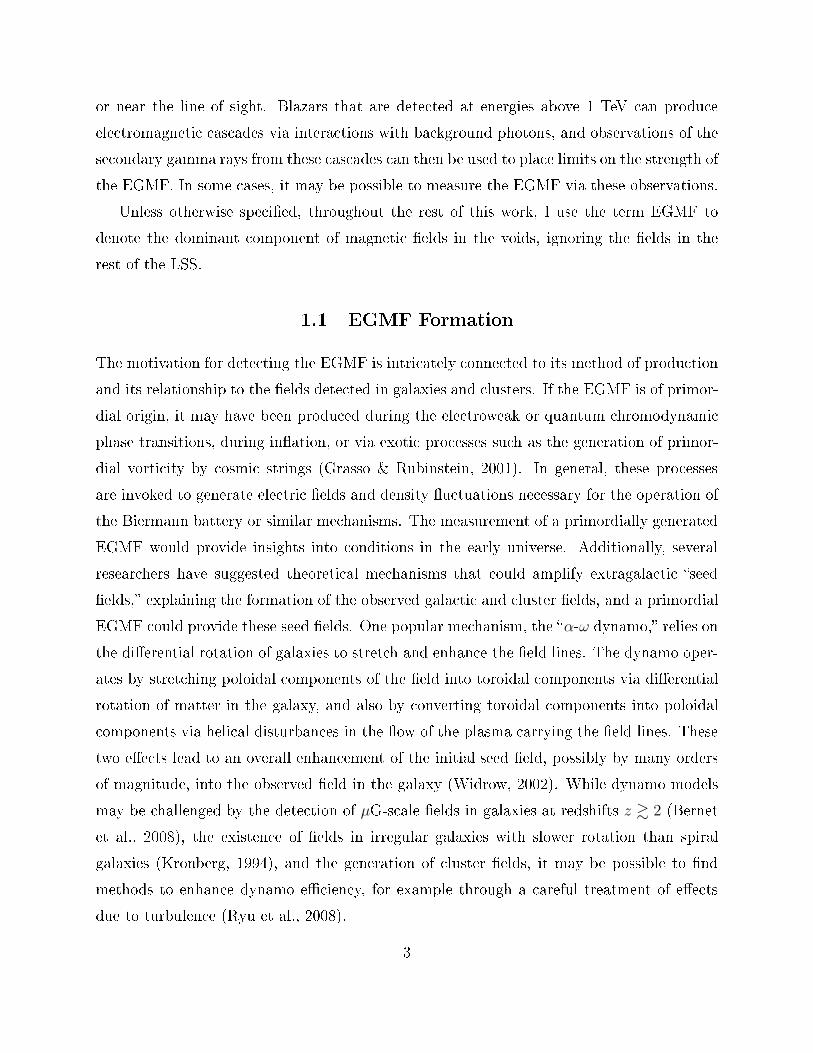
EGMF Correlation Length [Mpc]

-1310 -1110 -910 -710 -510 -310 -110 10 310 510

EG

MF

Str

eng

th [

Gau

ss]

-1210

-1110

-1010

-910

-810

-710

-610

-510

-410

Zeeman Splitting

Mag

net

ic D

iffu

sio

n

Faraday Rotation

Ho

rizon

CMB

BBN

Figure 1.1: Existing limits on the EGMF strength and orrelation length, adaptedfrom Neronov & Semikoz (2009).dependent Faraday rotation of left and right ir ularly polarized light provide a stronger onstraint on B (Kronberg & Perry, 1982; Blasi et al., 1999).It is possible to limit the present-day strength of a primordially generated EGMF dueto the absen e of an observed global anisotropy in measurements of the osmi mi rowaveba kground (CMB). This limit depends on the unknown power spe trum of the EGMF, so itis displayed in the gure as an upper limit on an EGMF uniform over all spa e. Additionally,the su ess of big bang nu leosynthesis limits the EGMF be ause a primordial magneti eldwould a elerate the expansion of the universe, leading to the overprodu tion of helium andthe underprodu tion of heavier elements (Grasso & Rubinstein, 2001; Widrow, 2002). Thislimit obviously applies only to a primordially generated eld and appears as a light grayex lusion region in Figure 1.1. 6

1.4 Measuring the EGMFFigure 1.1 la ks any lower bounds on the strength of the EGMF. The observations thereforepermit a very wide range of a eptable values for B; logarithmi ally speaking, this range isunbounded from below. Until re ently, no lower limits on the strength of the EGMF existed.However, the re ent development of experimental gamma-ray astrophysi s has opened up anew window on the universe, through whi h glimpses of the EGMF are beginning to appear.These glimpses arise through the inuen e of the EGMF on ele tromagneti as ades thatdevelop in extragala ti spa e due to the intera tion of primary gamma rays with the isotropi populations of ba kground photons. Aharonian et al. (1994) pointed out that these as adeswould appear as a halo of extended emission around otherwise pointlike sour es of gammarays due to the a tion of the EGMF, and Plaga (1995) realized that time delays, or e hosfrom aring sour es ould probe very small EGMF strengths, possibly as low as 10−24 Gauss.More re ently, several studies have explored the dependen e of the extended as adeemission on the EGMF, either through Monte Carlo simulations (Eungwani hayapant &Aharonian, 2009; Elyiv et al., 2009; Dolag et al., 2009) or analyti models with simplifyingapproximations (Neronov & Semikoz, 2007, 2009; Ahlers, 2011). Neronov & Semikoz (2009)also investigated the sensitivity of gamma-ray teles opes to the EGMF signature in the as ades by studying the pair produ tion and inverse Compton intera tions under severalsimplifying assumptions. In addition, several other resear hers hara terized the as adetime delays in the ontext of gamma-ray bursts (I hiki et al., 2008; Murase et al., 2008).Lower limits on the as ade ux due to gamma ray observations have lately begun toappear in the literature. Combined with the upper limits from Figure 1.1, these lower limits an be onstrued, with aveats, as a positive dete tion of the EGMF. Neronov & Vovk(2010) studied observations of the spe tra from three extragala ti sour es to derive theselower limits, and other authors have employed similar methods (Tave hio et al., 2010b;Taylor et al., 2011; Huan et al., 2011). Dermer et al. (2011) pointed out that the period ofa tivity of the sour es should be taken into a ount in setting these limits, and Essey et al.(2011) onsidered the modi ation of the limits in the ase that the gamma-ray sour es arealso sour es of osmi -ray nu lei. A laim of a positive dete tion of the EGMF by Ando &Kusenko (2010), however, turned out more likely to be an instrumental artifa t (Neronovet al., 2011). 7

In this work, I aim to explore this new te hnique to a ess the properties of the EGMF.Spe i ally, I build upon previous resear h, whi h used only the spe tral information avail-able from models of the as ade to onstrain the EGMF, by sear hing for the extended haloof se ondary gamma rays expe ted around otherwise pointlike sour es of gamma rays. Chap-ter 2 des ribes the ba kground photon populations that initiate and sustain the as ades andsummarizes the aspe ts of pair produ tion and inverse Compton s attering that are relevantto the development of ele tromagneti as ades in extragala ti spa e. A brief review of thesour es and dete tors used in this new method appears in Chapter 3, followed in Chapter 4by a des ription of a semi-analyti model that presents a on eptually lear but statisti allypowerful method to hara terize the spe tra of the as ades. Chapters 5 and 6 are respe -tively dedi ated to the des ription of a detailed Monte Carlo simulation of the as ade andthe appli ation of that simulation to sear h for the energy-dependent morphologi al imprintof the EGMF on the as ades. I on lude in Chapter 7 with a dis ussion of the relevan e ofa strong EGMF and opportunities for future work.

8

CHAPTER 2EXTRAGALACTIC BACKGROUNDS AND INTERACTIONSEle tromagneti as ades developing in extragala ti spa e suer three primary intera tions:pair produ tion of gamma rays on the isotropi photon ba kgrounds, inverse Compton s at-tering of ba kground photons by high-energy ele trons and positrons, and Lorentz for eintera tions between the harged leptons and the EGMF. The development of an under-standing of the hara teristi s of the as ade is riti al for extra ting information on theEGMF from gamma-ray observations. In this hapter, I summarize the relevant isotropi photon ba kgrounds and fundamental physi s intera tions that initiate and sustain the ex-tragala ti ele tromagneti as ades.2.1 Isotropi Ba kgroundsThe dominant photon ba kgrounds inuen ing the as ade are the osmi mi rowave ba k-ground (CMB) and the extragala ti ba kground light (EBL). As the remnant radiationfrom the early universe at the time of de oupling, the CMB is remarkably well measured andfollows a nearly perfe t bla kbody spe trum (Mather et al., 1994). In ontrast, attempts tomeasure the EBL are ompli ated by the presen e of strong foreground ontributions fromthe Galaxy and from zodia al light due to dust in the solar system (Mazin & Raue, 2007).Figure 2.1 summarizes re ent measurements of the EBL based on the work of a vari-ety of resear hers. The high-energy peak of the EBL arises due to the integrated opti alemission from galaxies throughout the star-forming history of the universe, while absorptionand thermal re-radiation of that opti al emission by dust generates the peak at lower en-ergies (Mazin & Raue, 2007). In general, dire t measurements of dark sky regions an be ontaminated by the foreground emission and should be interpreted onservatively as upperlimits on the EBL density. Similarly, measurements of galaxy ounts must extrapolate those ounts below the onfusion limit and should therefore be onsidered onservatively as lowerlimits. As indi ated in Figure 2.1, at some energies the range of allowed values for the EBLenergy density an vary by nearly an order of magnitude between these lower and upperlimits. In order to draw onservative on lusions based on the as ade ux generated fromele tromagneti intera tions with the EBL, I adopt the EBL model of Fran es hini et al.9

Energy [eV]-210 -110 1 10

]-3

dn

/dE

[eV

cm

2E

-410

-310

-210

-110

SpitzerCOBE DIRBEHubbleISOOther

Figure 2.1: Measurements and onstraints on the EBL at z = 0, adapted from Mazin &Raue (2007), along with the z = 0 EBL model from Fran es hini et al. (2008). The datapoints are olored a ording to the instrument used to derive them.(2008), whi h is shown in Figure 2.1 to follow the EBL lower limits reasonably well. Theresults from this model are onservative be ause the total amount of as ade emission, whi h arries the signal of the EGMF, is smaller than for a model with a higher density of EBLphotons. Still lower models, su h as that of Gilmore et al. (2009) exist, and Vovk et al.(2012) have shown that su h models likely ae t on lusions about the EGMF by a fa torof at most a few.When redshift due to the expansion of spa e is a ounted for, the CMB energy densityρCMB evolves as a radiation energy density:

ρCMB(z) = (1 + z)4ρCMB(0). (2.1)10

Energy [eV]-410 -310 -210 -110 1 10

]-3

dn

/dE

[eV

cm

2E

-410

-310

-210

-110

1

10

z = 0

z = 0.2

z = 0.4

z = 0.6

z = 0.8

z = 1

Figure 2.2: Re ent history of the CMB and EBL from the model of Fran es hini et al. (2008).Be ause the EBL in orporates emission generated throughout the history of the universe,however, its evolution is more ompli ated sin e sour e terms must be a ounted for. There ent history, out to z = 1, of both the CMB and the EBL from Fran es hini et al. (2008)appears in Figure 2.2, in whi h the deviation of the EBL's evolution from the simple s alingof Equation 2.1 is evident.Figure 2.2 shows only a restri ted portion of the ba kground photon spe trum. At lowerenergies, one expe ts to nd an isotropi population of radio photons, while at higher energiesan isotropi x-ray ba kground appears. Due to its low number density ompared to the CMBand even the EBL, the x-ray ba kground is largely irrelevant to as ades initiated by gammarays at the TeV s ale (Gould & S hréder, 1967). The energies of photons in the radioba kground are generally far too low to provide pair produ tion targets for gamma rays withenergies below 105 TeV, and their inuen e on the energies and traje tories of the ele trons11

and positrons in the as ades will be negligible for the same reason.2.2 Pair Produ tionIn the absen e of pair produ tion intera tions, gamma rays from extragala ti sour es wouldtravel dire tly to Earth without attenuation, and while the benet to gamma-ray obser-vations of extragala ti obje ts would be undeniable, the inuen e of the EGMF on the as ades would be impossible to measure be ause there would be no as ades. This se -tion summarizes the pair produ tion intera tion in the ontext of the development of theextragala ti as ades. 2.2.1 Kinemati sDiagrams depi ting the relevant kinemati s for the pair produ tion intera tion appear inFigure 2.3, with the situation in the lab frame prior to intera tion being shown in the upperleft. It is onvenient to introdu e the variable q, given by1

q=

1

2

Eǫ

m2c4(1 − cos θ), (2.2)where E and ǫ are the energies of the primary gamma ray and target photon, respe tively,and θ is the angle between their traje tories, as shown in Figure 2.3(a). Sin e q is related tothe Mandelstam s via q = 4m2c4/s, the threshold ondition for pair produ tion √

s ≥ 2mc2 an be expressed as q ≤ 1. As q is positive by onstru tion, its range of validity is thereforem2c4/Eǫ ≤ q ≤ 1. This range makes it lear that it is possible to nd ombinations of Eand ǫ for whi h pair produ tion does not o ur, namely √

Eǫ ≤ mc2.Following a boost ~β to the enter of momentum frame, the ollision be omes head-on,as shown in Figure 2.3(b), with both photon energies given by E′. A ording to Protheroe(1986), the appropriate boost speed isβ =

E cosφ+ ǫ cos(θ − φ)

E + ǫ, (2.3)

12

LAB

E

∈

β

θ

φ

(a)

CM

(b)

E’ E’

CM

β-

+e

-e’eE

’eE

’ψ’α

(c)

LAB

+e

-e

(d)Figure 2.3: Kinemati s of the pair produ tion intera tion. (a) Photons in the lab frame priorto intera tion, with boost ve tor ~β to the enter of momentum frame indi ated. (b) Aftera boost into the enter of momentum frame but still prior to intera tion. ( ) Ele tron andpositron produ ed in the enter of momentum frame, with boost ve tor -~β ba k to the labframe indi ated. (d) The boost ba k to the lab frame results in the leptons propagating atsmall angles relative to the initial dire tion of the gamma ray.with the boost angle φ relative to the primary gamma ray's dire tion spe ied bytanφ =

ǫ sin θ

E + ǫ cos θ. (2.4)13

q0 0.1 0.2 0.3 0.4 0.5 0.6 0.7 0.8 0.9 1

Tσ / γγσ

0

0.05

0.1

0.15

0.2

0.25

0.3

Figure 2.4: Total ross se tion for pair produ tion as a fun tion of q.The appropriate boost fa tor for a head-on ollision (cos θ = −1) in the lab frame betweena high-energy gamma ray and a low-energy ba kground photon (E ≫ ǫ) is thereforeβ =

E − ǫ

E + ǫ≈ 1 − 2

ǫ

E. (2.5)This orresponds to a Lorentz fa tor of γ ≈

√

E/4ǫ. In general, via straightforward boostme hani s, the angle ψ′ is given bytanψ′ =

(E + ǫ) sin θ

γ(E − ǫ)(1 − cos θ), (2.6)and this permits a return to the lab frame following the omputation of the kinemati s inthe enter of momentum frame. 14

Working in the enter of momentum frame, Jau h & Rohrli h (1976) nd that the spin-independent dierential ross se tion for pair produ tion isdσγγ

dxα′

=3

8σT

q√

1 − q

2

1 − (1 − q)2x4α′ + 2q(1 − q)(1 − x2

α′)[

q − (1 − q)x2α′

]2, (2.7)where σT ≈ 6.65 × 10−25 m2 is the Thomson ross se tion and xα′ = − cosα′, with α′ theangle between the outgoing ele tron and the dire tion of the primary gamma ray, as shownin Figure 2.3( ). The total ross se tion for pair produ tion an be found by integratingEquation 2.7 over xα′ to obtain

σγγ(q) =3

8σT q

[(

1 + q − 1

2q2)

ln

(

1 +√

1 − q

1 −√1 − q

)

− (1 + q)√

1 − q

]

, (2.8)whi h is plotted in Figure 2.4. The fun tion σγγ(q) has a peak at q ≈ 0.508, whi h an beinterpreted via Equation 2.2 either as a preferred target energy ǫ given the ollision angle θor a preferred ollision angle given the target energy. For a head-on ollision, the preferredtarget energy for a primary photon with energy ETeV TeV is given byǫeV ≈ 1

2ETeV , (2.9)where ǫeV is the ba kground photon energy in eV.2.2.2 Produ t Angles and EnergiesIn the enter of momentum frame, the ele tron and positron are ea h produ ed with energy√s/2 due to onservation of momentum. This translates to a speed of

cβ′e = c√

1 − q. (2.10)At the most likely value q ≈ 0.508, β′e ≈ 0.7. Under the assumption of a primary gammaray with very high energy intera ting via head-on ollision with a low-energy ba kgroundphoton, the approximation from Equation 2.5 an be used to ompute the angle α that theele tron's lab frame traje tory makes with respe t to the dire tion of the primary gamma15

’αcos-1 -0.8 -0.6 -0.4 -0.2 0 0.2 0.4 0.6 0.8 1

Tσ / ’α

/ d

xγγσd

0

0.05

0.1

0.15

0.2

0.25

q = 0.1q = 0.25q = 0.508q = 0.75q = 0.9

Figure 2.5: Pair produ tion dierential ross se tion, for sele t values of q, as a fun tion ofthe ele tron emission angle in the enter of momentum frame.ray. A simple appli ation of the Lorentz transformation yieldstanα ≈ 2

√

ǫ

E

β′e sinα′

β′e cosα′ − 1. (2.11)The angle α is thus suppressed by the fa tor √ǫ/E, whi h is small, in the range of 10−6a ording to Equation 2.9. This order-of-magnitude al ulation suggests that the produ tsof pair produ tion intera tions in the extragala ti as ade are generally ollimated in thedire tion of the primary gamma ray, provided that ba kground photons exist in su ientnumbers at the favored target energy.

16

Under the same approximation, the energy of the ele tron in the lab frame appears asEe = E′

eγ(1 − ββ′e cosα′) ≈ 1

2

√

E

ǫ

√s

2(1 − β′e cosα′) =

1

2E(1 − β′e cosα′). (2.12)The spe i value of the energy depends on β′e (and thereby q through Equation 2.10), andthe distribution of cosα′, whi h an be obtained from the dierential ross se tion spe iedby Equation 2.7. Figure 2.5 shows the distribution of cosα′ for several values of q. Smallvalues of q tend to favor extreme values for cosα′, while large values tend toward a atterdistribution. For modest values of β′e and small values of cosα′, both of whi h are attainedat large values of q, Equation 2.12 indi ates that the primary gamma ray's energy is splitevenly between the produ t ele tron and positron to a good approximation. As q de reases,

β′e approa hes 1 while cosα′ approa hes ±1, indi ating that one of the leptons re eives mostof the energy of the primary gamma ray, while the other lepton be omes far less energeti .At the most likely value q ≈ 0.508, | cosα′| attains an average value of approximately 0.56,and the more energeti lepton re eives approximately 0.7 of the primary gamma ray's energy.For omparison, at q = 0.9 the more energeti lepton has only 0.58 of the primary gammaray's energy, and at q = 0.1 the fra tion is 0.84.While the al ulations performed in this se tion apply stri tly only to head-on ollisions,they an be straightforwardly generalized to ases where cos θ 6= −1 via an appropriate ad-justment of either E or ǫ given a value for q. In this sense, they should apture the essen eof the physi s at the order-of-magnitude level of a ura y. In general, the Monte Carlo sim-ulation des ribed in Chapter 5 employs the full distributions instead of the approximationsmade in this se tion. 2.3 Inverse Compton S atteringThe se ond part of the as ade involves the inverse Compton s attering pro ess, whi h isthe same as the Compton s attering pro ess in the limit of large the ele tron energy in thelab frame.17

LAB

E

∈

θ

(a)

CM

(b)

’θω

CM

’α

’ψ

’ω

’eE

(c)

LAB

eE

γE

(d)Figure 2.6: Kinemati s of the inverse Compton s attering intera tion. (a) An energeti ele tron in the lab frame intera ts with a ba kground photon. (b) After a boost into the enter of mass frame, the ele tron is at rest with the photon in ident prior to intera tion.( ) Following intera tion, the ele tron and photon s atter. (d) Similar to pair produ tion,a boost ba k to the lab frame results in the ollimation of the parti les along the ele tron'sinitial traje tory. 2.3.1 Kinemati sThe kinemati s of inverse Compton s attering diers signi antly from that of pair produ -tion. Figure 2.6 illustrates the relevant aspe ts of the pro ess. It is onvenient to introdu e18

the variable x, given byx = 2

Eǫ

m2c4(1 − β cos θ), (2.13)where E and ǫ are respe tively the ele tron energy and photon energy in the lab frame, θis the angle between the parti les as indi ated in Figure 2.6(a), and βc is the speed of theele tron in the lab frame before the intera tion. Compton s attering is well studied in the enter of mass frame in whi h the ele tron is at rest, so the natural hoi e is to boost at speed

β along the ele tron's lab-frame traje tory. Following this boost, the ba kground photonhas energy ω1, measured in terms of the ele tron mass mc2, as shown in Figure 2.6(b). Theintera tion imparts some energy to the ele tron, after whi h the photon's new energy is ω′(Figure 2.6( )). The angle α′ spe ies the angle of dee tion of the ba kground photon withrespe t to its initial traje tory in the enter of mass frame. As with pair produ tion, whenthe boost ba k to the lab frame is performed, the parti les be ome ollimated along theinitial traje tory of the ele tron. This is depi ted in Figure 2.6(d).In ontrast to the pair produ tion intera tion, inverse Compton s attering does not in-volve the reation of any new mass, so there is no threshold value for x as there was for q inthe previous se tion. The dierential ross se tion is straightforward to ompute (see Jau h& Rohrli h (1976) or Peskin & S hroeder (1995) for details) and is given bydσeγ

dxα′

=3

8σT

(

ω′

ω

)2 [ω′

ω+ω

ω′− 1 + x2

α′

]

, (2.14)where xα′ = − cosα′ again, and the relation between ω and ω′ is given by the famous formulafor the hange in wavelength of the Compton s attered photon:ω

ω′= 1 + ω(1 + xα′). (2.15)Integration of Equation 2.14 produ es the total ross se tion for inverse Compton s attering,

σeγ(x) =3

8σT

16x+ 32x2 + 18x3 + x4 − (16 + 40x+ 30x2 + 4x3 − 2x4) ln(1 + x)

x3(1 + x)2, (2.16)whi h appears in Figure 2.7. For small values of x, the ross se tion approa hes the Thomson1. It is straightforward to see that x = 2ω. 19

x0 1 2 3 4 5 6 7 8 9 10

Tσ /

eγσ

0

0.2

0.4

0.6

0.8

1

Figure 2.7: Total ross se tion for inverse Compton s attering. ross se tion σT .Figure 2.7 demonstrates that small values of x are favored in inverse Compton s attering.A ording to Equation 2.13, this translates to ba kground photons with lower energies and,somewhat ounterintuitively, traje tories in line with the ele tron's own traje tory. However,due to the in lusion of a fa tor proportional to the relative speed between the photon andele tron when we ompute the intera tion rate, these photons will only be important in thes attering if the energy of the ba kground photon be omes omparable to the energy of theele tron and they an generally be disregarded (Blumenthal & Gould, 1970). The dierential ross se tion from Equation 2.14 appears in Figure 2.8, whi h highlights the in reased rossse tion for small values of ω (and therefore small values of x). As the target photon energyis in reased, not only does the ross se tion de rease, but the distribution of the angle α′through whi h the photon is dee ted away from its initial traje tory be omes strongly20

’αcos-1 -0.8 -0.6 -0.4 -0.2 0 0.2 0.4 0.6 0.8 1

Tσ / ’α

/ d

x eγσd

0

0.1

0.2

0.3

0.4

0.5

0.6

0.7 = 0ω

= 0.1ω

= 1ω

= 10ω

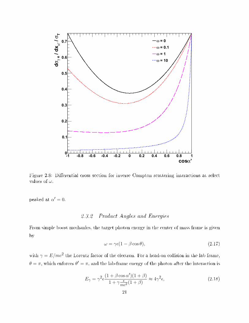
Figure 2.8: Dierential ross se tion for inverse Compton s attering intera tions at sele tvalues of ω.peaked at α′ = 0. 2.3.2 Produ t Angles and EnergiesFrom simple boost me hani s, the target photon energy in the enter of mass frame is givenbyω = γǫ(1 − β cos θ), (2.17)with γ = E/mc2 the Lorentz fa tor of the ele tron. For a head-on ollision in the lab frame,

θ = π, whi h enfor es θ′ = π, and the lab-frame energy of the photon after the intera tion isEγ = γ2ǫ

(1 + β cosα′)(1 + β)

1 + γ ǫmc2

(1 + β)≈ 4γ2ǫ, (2.18)21

where the approximation is valid in the limit of small s attering angles cosα′ ≈ 1 andsubje t to the Thomson limit √Eǫ ≪ mc2. Equation 2.18 is a general upper bound on theprodu ed gamma ray's energy in all regimes. A full treatment of all the in ident angles foran isotropi distribution of ba kground photons amends this approximation in the Thomsonlimit to (Blumenthal & Gould, 1970)Eγ ≈ 4

3γ2ǫ. (2.19)Equation 2.19 inspires an approximation to the rate of hange of the ele tron's energy as theprodu t of the energy loss per intera tion and the intera tion rate for a highly relativisti ele tron, cσTnCMB,

mc2dγe

dt≈ −4

3γ2e ǫ0cσTnCMB, (2.20)where ǫ0 is the energy of the peak of the CMB. In the Thomson limit, even though thein rease in the photon's energy is enormous (by a fa tor of γ2 from the relativisti ele tron),the fra tional loss of energy of the ele tron is of order Eǫ/m2c4 and therefore small. Thisis not the ase in the Klein-Nishina regime, when the ele tron loses a substantial amount ofits energy to the photon and the approximation of Equation 2.18 is no longer valid.Equation 2.19 ensures that the se ondary photons appear at gamma-ray energies. Forexample, an ele tron with energy 1 TeV (presumably generated by a pair produ tion eventfrom a primary gamma ray with energy 2 TeV) has a Lorentz fa tor of γ ≈ 2 × 106. Itsintera tion with the peak of the CMB at energy 0.6 meV produ es a se ondary gamma raywith approximate energy 3 GeV by Equation 2.19.As with pair produ tion, the inverse Compton s attered produ ts are highly ollimatedalong the initial ele tron traje tory. From simple boost me hani s, the nal lab-frame an-gle θγ that the produ t gamma ray makes with the ele tron traje tory is given withoutapproximation by

cos θγ =β + cos(θ′ − α′)

1 + β cos(θ′ − α′). (2.21)For a head-on ollision at high energy, the angle is suppressed by a fa tor of 1/γ,

θγ ≈ 1

γ

√

cosα′

1 − cosα′, (2.22)22

provided that α′ is not espe ially small.2.4 The Mean Free Path for Intera tionsThe kinemati s of both the pair produ tion and inverse Compton pro esses determines theenergy distributions of gamma rays in the extragala ti as ades. Naturally, the intera tionlengths of these pro esses inuen e the as ade geometry. In this se tion, I onsider themean free paths of the two pro esses separately and then dis uss their role in the as ade.2.4.1 Pair Produ tionFor an arbitrary density of isotropi ba kground photons, nǫ(ǫ), spe ied in units of photonsper energy per volume, the mean free path for pair produ tion λγγ appears as (Protheroe,1986)1

λγγ=

∫ ∞

0dǫ

2nǫ(ǫ)m4c8

E2ǫ2

∫ 1

qmin dqσγγ(q)

q3≡∫ ∞

0dǫQγγ(ǫ). (2.23)The threshold value qmin = m2c4/Eǫ. Equation 2.23 is a urate for small redshifts but anbe straightforwardly generalized to ases where z 6= 0. The integrand Qγγ(ǫ) is large forba kground energies ǫ that are likely to initiate a pair produ tion intera tion, so it may be rudely interpreted as the odds for a primary gamma ray with energy E to intera t with aba kground photon of energy ǫ, given the isotropi density nǫ(ǫ).Figure 2.9 shows Qγγ(ǫ) as a fun tion of ba kground energy for several values of E. Fromthe gure, it is evident due to the pair produ tion threshold ondition that primary gammarays with energies under 100 TeV intera t almost ex lusively with the EBL. As the energy ofthe primary gamma ray de reases, the pair produ tion threshold di tates that the intera tionmust o ur with ba kground photons of in reasingly higher energy, so that primary gammarays at 1 TeV intera t primarily with the high-energy opti al peak of the EBL. Additionally,it is apparent from the gure that the intera tion length de reases with primary gamma-ray energy, at least in the range from 100 GeV to 100 TeV. The reason for this de rease isapparent in Figure 2.2. The energy densities in the infrared and opti al peaks of the EBLare approximately the same, but the energy of an average photon in the two peaks diersby two orders of magnitude. Consequently, the preferred targets for 100-TeV primaries areabout 100 times more numerous than those for 1-TeV primaries, and the mean free path is23

Background Energy [eV]-410 -310 -210 -110 1 10

]-1

pc

-1)

[eV

∈( γγIn

teg

ran

d Q

-1110

-1010

-910

-810

-710

-610

-510

-410

-310 ]-3

dn

/dE

[eV

cm

2B

ackg

rou

nd

Sp

ectr

um

E

-310

-210

-110

100 TeV10 TeV1 TeV100 GeVBackgrounds

Figure 2.9: The integrand of Equation 2.23 as a fun tion of ba kground energy, along withthe isotropi ba kground photon distribution.therefore about 100 times shorter.2.4.2 Inverse Compton S atteringAgain referring to Protheroe (1986), I nd the mean free path for inverse Compton s atteringλeγ to be

1

λeγ=

∫ ∞

0dǫnǫ(ǫ)m

4c8

8βE2ǫ2

∫ x+

x−dxxσeγ(x) ≡

∫ ∞

0dǫQeγ(ǫ), (2.24)where the limits x± = 2Eǫ(1 ± β)/m2c4 arise from setting cos θ = ±1 in Equation 2.13.Figure 2.10 plots the integrand Qeγ(ǫ), again with the ba kground energy densities. It isobvious from the gure that inverse Compton s attering pro eeds primarily via intera tionswith the CMB, although some intera tions with the infrared peak of the EBL may o ur. The24

Background Energy [eV]-410 -310 -210 -110 1 10

]-1

pc

-1)

[eV

∈( γeIn

teg

ran

d Q

-910

-810

-710

-610

-510

-410

-310

-210

-110

1

10 ]-3

dn

/dE

[eV

cm

2B

ackg

rou

nd

Sp

ectr

um

E

-310

-210

-110

100 TeV1 TeV10 GeVBackgrounds

Figure 2.10: The integrand of Equation 2.24 as a fun tion of ba kground energy. urves in Figure 2.10 more losely follow the ba kground densities than those of Figure 2.9due to the absen e of a preferred intera tion energy for this pro ess. They are also remarkablysimilar over a very wide ele tron energy range from 10 GeV to 100 TeV, at whi h pointthe ross se tion of Equation 2.16 begins to diverge from the Thomson limit. Althoughintera tions with the EBL o ur far less frequently than with the CMB, the ba kgroundenergies, and onsequently the produ t photon energies, are mu h higher and a single EBLintera tion an be important to the development of the as ade. For example, for a 20-TeVele tron, the transition to the Klein-Nishina regime o urs at a ba kground photon energyof about 10 meV, well above the CMB but well within the infrared peak of the EBL.25

Particle Energy [TeV]-210 -110 1 10 210 310 410

Mea

n F

ree

Pat

h [

pc]

210

310

410

510

610

710

810

910

1010

Pair production on EBLPair production on CMBPair production totalCompton scattering on EBLCompton scattering total

Horizon Scale

Cluster Scale

Galaxy Scale

Figure 2.11: The mean free path λ as a fun tion of primary energy for pair produ tionand inverse Compton s attering. Average size s ales for galaxies, lusters, and the universehorizon are also indi ated.2.4.3 Inuen e of the Cas adesFigure 2.11 plots the mean free path as a fun tion of primary parti le energy for boththe pair produ tion and inverse Compton s attering pro esses. As shown in the gure,primary gamma rays below about 200 GeV will stream freely through the universe with anintera tion length greater than a Hubble radius. Above 100 TeV, the primary gamma rayswill intera t on luster-s ale distan es, where the lo al luster magneti elds are strongand any pairs produ ed are qui kly isotropized. Primary gamma rays between 200 GeV and100 TeV will produ e an extragala ti as ade of ele trons that intera t with the CMB onkp -s ale distan es. Sin e the energy loss of the ele trons is proportional to the square oftheir energy via Equation 2.20, however, the number of these intera tions in reases as the26

energy de reases, and the ele trons may propagate mu h farther than 1 kp .The role of the extragala ti as ades is thus to onvert gamma rays at the TeV-s aleand above into gamma rays at the GeV s ale, whi h an freely propagate throughout theuniverse. Depending on the distan e between the sour e and the observer, se ondary gammarays with energies signi antly in ex ess of 200 GeV an intera t again and the as ade ango through multiple generations of parti les. The dee tions of the ele trons and positronsover their traje tories reate time delays, or e hos, and extended emission, or halos,of se ondary, as aded gamma rays around otherwise pointlike sour es. The spe tral andspatial properties of these e hos and halos an be used to extra t information about theEGMF, whi h a ts via the Lorentz for e on the ele trons and positrons in the as ade.2.4.4 Redshift GeneralizationsChapter 5, whi h des ribes the development of a Monte Carlo simulation for hara terizingthe as ade, relies on the generalization Equations 2.23 and 2.24 to a ount for redshift.These generalizations appear as1

λγγ=

∫ ∞

0dǫ0

2c(1 + zi)2m4c8

H0E2i ǫ

20

∫ zi

zf

dznǫ [(1 + z)ǫ0; z]

(1 + z)4Q(z)

∫ 1

qmin(z)dqσγγ(q)

q3, (2.25)for pair produ tion and

1

λeγ=

∫ ∞

0dǫ0

m4c9

8H0ǫ20

∫ zi

zf

dznǫ [(1 + z)ǫ0; z]

β(z) [E(z)]2 (1 + z)2Q(z)

∫ x+(z)

x−(z)dxxσeγ(x), (2.26)for inverse Compton s attering. In Equation 2.25, Ei is the energy of the gamma ray atits initial redshift zi, zf is the nal redshift, ǫ0 is the present-day energy of the ba kgroundphoton, qmin(z) generalizes to

qmin(z) =(1 + zi)m

2c4

(1 + z)2ǫ0Ei, (2.27)

H0 ≈ 70 km/s/Mp is the Hubble parameter, and Q(z) is the osmologi al fa torQ(z) =

√

(1 + z)4ΩR + (1 + z)3ΩM + ΩΛ + (1 − ΩC)(1 + z)2, (2.28)27

Source Earth

Dθ

CθSθ

L

L’

Figure 2.12: Geometry relevant to the extragala ti as ades, following Dermer et al. (2011).with ΩR, ΩM , ΩΛ, and ΩC respe tively the radiation, matter, osmologi al onstant, and urvature densities in units of the riti al density ρC (Kolb & Turner, 1990). We adoptthe standard ΛCDM osmology with ΩR = 0, ΩM = 0.3, ΩΛ = 0.7, and ΩC = 1. InEquation 2.26, the redshift evolution of the ele tron's energy is given generally by [E(z)]2 =

[p(z)]2 c2 −m2c4, wherep(z)c =

1 + z

1 + zi

√

E2i −m2c4, (2.29)and β(z) = cp(z)/E(z). The limits on the x integration are

x±(z) = 2(1 + z)E(z)ǫ0m2c4

[1 ± β(z)] . (2.30)2.5 The Lorentz For eThe EGMF inuen es the as ade ele trons and positrons dire tly through the Lorentzfor e. A relativisti ele tron with Lorentz fa tor γ in a onstant magneti eld follows aspiral traje tory with Larmor radiusrL =

mc√

γ2 − 1

eB=

peeB

, (2.31)where e is the harge of the positron and B is the omponent of the eld strength perpen-di ular to the motion of the parti le. The momentum of the ele tron is pe. As the ele tron28

propagates through a distan e D along this traje tory, then, its dee tion θD isθD =

D

rL=

eBD

mc√

γ2 − 1. (2.32)Equation 2.32 may be used to approximate the size of the as ade halo. The relevantgeometry for an extragala ti sour e at a distan e L is shown in Figure 2.12. In the gure, aprimary gamma ray is emitted at an angle θS relative to the line of sight to the extragala ti sour e. The primary gamma ray travels a distan e L′ before intera ting. After the ele tron isdee ted through an angle θD, the se ondary photon is emitted and arrives at the observerwith an angle θC relative to the sour e. The angle θC is obviously θC = θD − θS andapproximates the size of the halo.For small angles, LθC ≈ L′θD. A ording to Figure 2.11, a 1-TeV gamma ray willtravel about 400 Mp before intera ting. For a sour e of 1-TeV gamma rays at a distan eof 1000 Mp , then, θC ≈ 0.4θD. After intera ting, the gamma ray produ es an ele tronwith energy of about 500 GeV, orresponding to γ ≈ 106. On average, this ele tron willintera t with the peak of the CMB at 0.6 meV, produ ing se ondary photons with energy800 MeV a ording to Equation 2.19. 300 su h intera tions o urring on e approximatelyevery kp will redu e the ele tron's energy by half, so with D ≈ 300 kp , Equation 2.32gives θC ≈ 0.2B/(10−15 Gauss). This very rough estimate suggests that 0.2 is not anunreasonable size to expe t for the halo due to the ee ts of the EGMF.2.6 Other Pro essesOur hara terization of the as ades depends on the assumption that inverse Compton s at-tering and pair produ tion are the dominant energy-loss hannels available to the parti les.In prin iple, pro esses su h as bremsstrahlung or syn hrotron radiation ould have a signi- ant impa t on the ele tron and positron energies. It is the aim of this se tion to show thatthese pro esses are negligible.Bremsstrahlung radiation is produ ed by harged-parti le intera tions with matter. Thedominant omponent of matter in extragala ti spa e is the warm-hot intergala ti medium(WHIM), whi h is primarily ionized hydrogen (Cen & Ostriker, 1999; Bykov et al., 2008).A ording to Blumenthal & Gould (1970), bremsstrahlung radiation an be thought of as29

inverse Compton s attering by high-energy ele trons on the virtual photons of the Coulombeld of the target proton, and in the high-energy limit, ele trons and positrons behave thesame, so I will treat only ele trons in this se tion. The energy loss rate from propagationthrough fully ionized hydrogen an be written asdγe

dt= 16αr20cneγe

[

ln(2γe) −1

3

]

, (2.33)where α ≈ 1/137 is the ne-stru ture onstant, ne is the ele tron number density of theWHIM, and r0 is the lassi al ele tron radius (σT = 8πr20/3). Blumenthal & Gould (1970)stress that Equation 2.33 does not ree t a ontinuous loss rate be ause the dominant en-ergy loss is due to photons that arry a signi ant fra tion of the ele tron's energy, so itshould not be integrated. Instead, we will ompare it to the energy loss rate due to inverseCompton s attering on the CMB, given by Equation 2.20, to determine the importan e ofbremsstrahlung radiation. The Thomson limit is appropriate be ause the energy loss due tothe CMB s ales with γ2e , faster than Equation 2.33, and Klein-Nishina losses will o ur evenfaster than losses in the Thomson limit. The ratio of the rates is thenRbrem ≡

(

dγedt

)brem(

dγedt

)CMB =9αmc2ne

[

ln(2γe) − 13

]

2πγeǫ0nCMB (2.34)Restri ting our interest to ele trons that produ e gamma rays above 100 MeV, we nd aminimum γe ≈ 3 × 105 via Equation 2.19 for an average CMB photon energy ǫ0 = 0.6meV, and writing ne = (1 + δ)nb in terms of the baryon density nb ≈ 0.045nC ≈ 2 ×10−7 m−3 (Kolb & Turner, 1990), I get

Rbrem ≈ 5 × 10−7(1 + δ). (2.35)If all of the baryons are in the WHIM, δ = 0 and even in this most optimisti ase thebremsstrahlung losses are relevant for fewer than one in every million ele trons. In reality,likely −δ is of order unity and bremsstrahlung losses are even more negligible.Ele trons an also lose energy due to syn hrotron radiation. Again following Blumenthal& Gould (1970), we note that that the energy-loss rate for syn hrotron radiation is analogousto the loss rate for inverse Compton intera tions on the CMB, with the energy density30

nCMBǫ0 repla ed by the eld energy density B2/2µ0, where µ0 is the magneti permeabilityof free spa e. The ee ts due to the magneti eld are equivalent to the CMB at a eldstrength BCMB given byBCMB =

√

2µ0ǫ0nCMB ≈ 1 µGauss, (2.36)and the signi an e of syn hrotron losses s ales as B2. Below 10−9 Gauss, then, the energylosses from syn hrotron radiation are even worse than for bremsstrahlung, so we negle tthem as well.

31

CHAPTER 3GAMMA-RAY SOURCES AND DETECTION TECHNIQUESHaving dis ussed the phenomenology of the extragala ti as ades, I now turn briey totheir dete tion. Three things are ne essary to observe the as ade: a gamma-ray dete tor,an ele tromagneti as ade, and an extragala ti sour e. The sour e must be of a lassthat is well understood, it must have a su iently large ux of TeV-s ale gamma rays toprodu e the as ade omponent, and it must be well measured in both the GeV and TeVenergy bands. There are not many options. Starburst galaxies are too faint to produ e anyappre iable as ade ux, and blazars are the only remaining extragala ti andidate sour e lass. Fortunately, sele t blazars meet all of the ne essary onditions.Gamma-ray observations of blazars are a omplished via two te hniques. At lower ener-gies, in the GeV band from 100 MeV to 100 GeV, spa e-based dete tors su h as the LargeArea Teles ope (LAT) on board the Fermi Gamma Ray Spa e Teles ope (Atwood et al.,2009), hereafter referred to as Fermi, dire tly dete t gamma rays passing through their in-strumented volume. Sin e the spe trum of every gamma-ray sour e de reases with in reasingenergy, eventually su h te hniques be ome ux-limited. In the TeV band, roughly from 100GeV to higher than 10 TeV, ground-based dete tors image the Cherenkov radiation from harged parti les in the air showers produ ed by the gamma rays' intera tions with the at-mosphere (Weekes, 1988). Known as Imaging Atmospheri Cherenkov Teles opes (IACTs),these dete tors boast mu h larger ee tive areas that ompensate for the de reasing ux,but only showers initiated by gamma rays with energies of 100 GeV and above are largeenough to be imaged. 3.1 BlazarsBlazars are a sub lass of a tive gala ti nu lei (AGN). The onventional pi ture of theAGN system omprises a host galaxy with a supermassive bla k hole at its enter and isdes ribed in detail by Urry & Padovani (1995). In the onventional pi ture, matter fallinginto the bla k hole forms an a retion disk from whi h jets of bulk material moving atrelativisti speeds emerge. Ele trons in the jets intera t with the lo al magneti eld toprodu e syn hrotron radiation, whi h is observed in the x-ray band and at lower energies.32

The ele trons an s atter either ambient photons from the host galaxy, CMB photons, ortheir own syn hrotron emission via inverse Compton s attering. The resulting s atteredphotons a quire gamma-ray energies. If the bulk motion is hara terized by a Lorentz fa torΓ with a typi al value around 10, a reasonable model for the high-energy emission f(E, θ)at the sour e is that of a boosted isotropi distribution with a power-law spe trum:

f(E, θ) ≡ dF

dEd cos θ= F0(1 − β cos θ)−α−1E−αe−E/EC , (3.1)where F is the ux in units of parti les per time per area, F0 is a normalization fa tor, βc isthe speed orresponding to Γ, β =

√

1 − 1/Γ2, θ is the emission angle of a photon relativeto the dire tion of the jet, and EC is an exponential uto energy that will be dis ussed ina moment.The hara teristi opening angle θ0 for the jet is approximated by θ0 ≈ 1/Γ. If the lineof sight to the AGN is signi antly larger than θ0, then most of the emission is beamed awayfrom the observer and the AGN is di ult to dete t in gamma rays. However, if the lineof sight angle is smaller than θ0, substantial gamma ray emission an be observed. In this ase, the AGN is alled a blazar be ause it is important to lassify things based on how theyappear.At energies above 1 TeV, the shape of the intrinsi spe trum given by Equation 3.1 annotbe observed dire tly be ause it is attenuated by intera tions with the EBL, as Figure 2.11demonstrates. Instead, a dire t omponent of gamma rays that survive the propagationpro ess is observed. The degree of attenuation depends on the energy and the distan e to thesour e. Most TeV-dete ted blazars inhabit a redshift range of 0.05 . z . 0.41, orrespondingto an approximate distan e range (assuming a at ΛCDM osmology) of 200 to 1500 Mp .For the nearer blazars, gamma rays above a few TeV will intera t in the spa e between theblazar and Earth, while in the extreme ase z ≈ 0.4, gamma rays with energies above a fewhundred GeV will intera t as well.Equation 3.1 in ludes an exponential uto energy EC , whi h fullls two purposes. First,when EBL attenuation is a ounted for through a deabsorption pro ess, many blazars arefound to have an intrinsi TeV spe tral index harder than 2, so there must be some termthat uts o the spe trum to avoid an innite energy atastrophe. The se ond purpose is1. See for example http://tev at.u hi ago.edu. 33

that, a ording to Figure 2.11, gamma rays with energies around 50 TeV and higher arelikely to intera t within the galaxy luster lo al to the host galaxy of the blazar. In that ase, the ele tron-positron pairs sample the µGauss-s ale luster eld instead of the EGMF,and they are rapidly isotropized in the eld before they undergo signi ant inverse Comptons attering. At any rate, what little emission that does rea h Earth from these pairs willbe indistinguishable from intrinsi emission unless the knowledge of the blazar spe trumis perfe t. This justies a maximum uto energy of 50 TeV, whi h I assume throughoutthe rest of this work, unless otherwise stated. In the absen e of other measurements of theblazar, I also assume a modest bulk Lorentz fa tor of Γ = 10 and a viewing angle of 0.The BL La ertae (BL La ) obje ts are the most prominent sub lass of blazars dete ted inthe TeV. Initially named for their resemblan e to the obje t BL La , these blazars are radio-loud AGN that la k strong emission or absorption features and are generally understood to beFanaro-Riley Class I galaxies (Urry & Padovani, 1995). BL La s are further lassied basedon the peak energy of their syn hrotron emission into low-frequen y-peaked BL La s (LBLs),intermediate-frequen y-peaked BL La s (IBLs), and high-frequen y-peaked BL La s (HBLs).A given BL La obje t an be lassied a ording to this s heme roughly quantitatively bydetermining the ratio of its radio ux to its x-ray ux. For IBLs this ratio takes on a valuenear 0.75, while LBLs lie above this value and HBLs lie below it (Fossati et al., 1998). Of41 BL La obje ts presently dete ted at TeV energies, 33 are of the HBL type.In sele ting a blazar for an EGMF study, one should be aware of the environment alongits line of sight, whi h should be dominated by void regions. If instead the line of sightpasses along a lament or through many lusters in the LSS, then there will be relativelyhigh luster and lament elds dee ting the leptons in the as ades and obs uring the signalfrom the EGMF. Due to the long intera tion length of the gamma rays and the short (sub-gala ti ) intera tion length of the pairs, it is not a problem to pass through some lustersbe ause they will ae t only a small subset of the pairs (Dolag et al., 2011); it is in the asewhen little of the line of sight traverses voids that problems arise. Fortunately, sin e theuniverse is dominated by voids (Pan et al., 2012), poor hoi es for the line of sight shouldbe rare.34

rayγ

calorimeter

front

back

+e -e

anti-coincidence

detector

Figure 3.1: S hemati diagram of the prin ipal omponents of the Fermi LAT.3.2 The Fermi InstrumentBlazar gamma rays in the energy range from 100 MeV to 300 GeV, where the signature ofthe EGMF on the extragala ti as ades is strongest, an be measured by the Fermi LAT.The LAT is a pair- onversion teles ope operating in survey mode with a eld-of-view of 2.4sr and an a eptan e of more than 2.2 m2 sr for energies above 1 GeV (Atwood et al., 2009).Fermi has been in operation sin e August 2008, so as of this writing more than three and ahalf years of data have been olle ted. These data are publi ly available as soon as they aretaken, and software for analyzing them is provided by the Fermi S ien e Support Center2.For the analysis presented in this work, I use version v9r23p1 of the s ien e tools, updated on1 November 2011, with the instrument response fun tion (IRF) orre tions P7SOURCE_V6,whi h in lude an updated on-orbit point-spread fun tion (PSF) for the instrument.Figure 3.1 provides a basi pi ture of gamma-ray dete tion in the LAT. In oming gammarays onvert to ele tron-positron pairs in the tungsten foil of the onverter, after whi h theele trons and positrons are tra ked by means of sili on strip dete tors in order to re onstru t2. http://fermi.gsf .nasa.gov/ss / 35

Energy [MeV]210 310 410 510

68%

Co

nta

inm

ent

Rad

ius

[Deg

rees

]

-110

1

10

Figure 3.2: Fermi LAT point-spread fun tion, adapted from Atwood et al. (2009). The urve is for gamma rays with normal in iden e onverting in the front part of the dete torare in luded, so the total PSF is somewhat larger.the gamma ray's dire tion. After exiting the tra ker, the ele trons and positrons deposit en-ergy in an ele tromagneti as ade in the alorimeter, whi h is made of CsI rystals and has adepth of 10 radiation lengths (Atwood et al., 2009), from whi h a measurement of the gammaray's energy an be inferred. The alorimeter also provides some tra king information, es-pe ially for gamma rays at the high-energy end of Fermi 's sensitivity. The onverter andtra ker ea h exist in two stages, a front stage with higher-resolution tra king and a ba kstage with lower-resolution tra king. Gamma rays are roughly equally likely to onvert inthe front stage as in the ba k. The entire instrument is surrounded by an anti- oin iden edete tor that provides ex ellent reje tion of the ba kground osmi -ray signal.Se tion 2.4.3 argued that the EGMF may reate as ade halos whose sizes are of order36

0.1 or larger. It is therefore important to have sub-degree resolution in the re onstru tionof the in oming gamma ray's dire tion, in order to resolve the features of the halo. The 68% ontainment radius of the LAT appears in Figure 3.2, demonstrating that this resoultion isattained for energies above several hundred MeV. The energy resolution of the LAT rangesfrom 8% to 18% over its sensitivity range, a hieving the best resolution between 1 and 10GeV (Atwood et al., 2009). More than 800 Fermi sour es are asso iated with blazars, nearly200 of whi h are BL La ertae (BL La ) obje ts with a syn hrotron omponent peaking at ahigh frequen y, above 1015 Hz (A kermann et al., 2011). Due to their generally hard spe traand substantial population of syn hrotron photons above a few eV, these high-frequen y-peaked BL La s (HBLs) are prime andidates for EGMF study be ause the extrapolation oftheir spe tra results in a high TeV-s ale ux.A atalog of existing sour es determined via surveys ondu ted by the Fermi team servesas a starting point for additional likelihood analyses (The Fermi-LAT Collaboration, 2011).In addition to numerous point sour es, the atalog in ludes 12 extended sour es, as wellas an isotropi diuse omponent and a detailed map of the Gala ti gamma-ray emission.Data analysis in Fermi pro eeds by proposing a sour e model and assessing the likelihoodof that model ompared to the likelihood of its absen e. This is a omplished by means ofa test statisti T , dened byT = −2 ln

(

L0

LGeV) , (3.2)where L0 is the likelihood from the null hypothesis of the model without the sour e and LGeVis the likelihood of the alternative hypothesis, in whi h a sour e present. This approa h isne essary be ause of the limited angular resolution of the LAT and the low number of gammarays olle ted. As long as the amount of data is su iently large, T is distributed in theabsen e of a sour e as a χ2(n), a χ2 distribution with n degrees of freedom, where n is thenumber of parameters hara terizing the proposed sour e.There are two standard methods for analyzing Fermi data, binned and unbinned. In thebinned ase, events are olle ted into energy bins, whereas in the unbinned ase ea h eventis treated separately. The two methods are expe ted to be equivalent in the limit of largestatisti s. Due to the faster pro essing time, in the rest of this work I use a binned methodunless otherwise stated. 37

3.3 Imaging Atmospheri Cherenkov Teles opesThe measureable ux of a blazar in general follows a power law with a spe tral index softerthan 1 and is therefore rapidly dropping with in reasing energy. Sin e Fermi is a dire tdete tion instrument, it is unable to measure gamma rays at the TeV s ale be ause it simplydoes not have a large enough area to inter ept an appre iable number of them. Additionally,any TeV-s ale gamma ray that did pass through the LAT would be likely to reate a showertoo large for the alorimeter to measure its energy a urately. However, it is exa tly the TeVs ale that must be measured in order to understand su iently the pro esses responsible forthe generation of the as ade. Without this information, any observed halo in the Fermienergy band would be di ult to interpret in the ontext of an EGMF. To a omplish theseTeV measurements, one must return to the ground.The Imaging Atmospheri Cherenkov Teles opes (IACTs) are sensitive to gamma rays inthe approximate energy range from 100 GeV to greater than 30 TeV. Instead of observing thegamma ray dire tly, these instruments image the Cherenkov radiation from ele tromagneti showers of parti les initiated by the gamma ray's intera tion with the atmosphere. The ur-rent generation of IACTs in ludes three teles opes that are presently operating, VERITAS,HESS, and MAGIC. Be ause these three instruments are qualitatively similar, I will fo ushere on a brief des ription of VERITAS in order to illustrate the IACT te hnique.In the atmosphere, harged parti les moving faster than the lo al speed of light emitCherenkov radiation. Atmospheri showers of parti les generated by very energeti gammarays produ e brief ashes of Cherenkov radiation with durations on the time s ales of a fewnanose onds (Weekes, 1988). This light an be olle ted by teles opes on the ground, whi hprodu e an image of the shower as it propagates through the atmosphere. The amountof light olle ted by the teles ope tra es the energy of the shower; more energeti gammarays will produ e more shower parti les and therefore more Cherenkov radiation. If multipleteles opes observe the shower, a stereo te hnique improves the re onstru tion of the initialgamma ray dire tion, as shown in Figure 3.3.The primary hallenge for the IACTs is to dis riminate the gamma-ray signal from theoverwhelming osmi -ray ba kground. This an be a omplished by means of image sele tion.Gamma-ray showers tend to be more ompa t than showers initiated by hadrons be ause, in ontrast to hadroni showers, they pro eed primarily via ele tromagneti hannels (Weekes,38

shower

Cherenkovlight

telescopesFigure 3.3: The stereo re onstru tion te hnique employed by VERITAS, HESS, and MAGIC.Cherenkov light from atmospheri showers is imaged by individual teles opes. Combining there onstru ted dire tions from several teles opes greatly improves the overall re onstru teddire tion of the gamma ray.1988). In general, gamma-ray showers tend to produ e narrower images in the IACTs, whi h an be dierentiated from the broader hadroni showers.The in rease in ee tive area granted by the Cherenkov imaging te hnique renders theIACTs more sensitive than Fermi to gamma rays when the primary energy is above ∼100GeV. VERITAS is sensitive to gamma rays in the energy range from 100 GeV to 30 TeV,with an ee tive area greater than 105 m2, an energy resolution of 10% to 20%, and a 68% ontainment radius of better than 0.14 (Hanna et al., 2008). Fermi and the IACTs aretherefore very omplementary instruments, espe ially from the point of view of studying theEGMF as ades. While Fermi an measure the as ade dire tly in the riti al GeV-s aleenergy range, the IACTs provide measurements of the dire t emission, ee tively onstraining39

the total TeV-s ale intrinsi emission that is responsible for the generation of the extragala ti as ade.Although the shape of a typi al osmi -ray-indu ed shower is distin t from that of atypi al gamma-ray-indu ed shower, the overwhelming majority of air showers are produ edby osmi rays. Some of these osmi rays produ e gamma-ray-like events, reating a ba k-ground that must be subtra ted (Hillas, 1996; Fegan, 1997). For this reason, IACTs inferthe gamma-ray ux of the sour e by employing a ba kground-subtra tion method in whi han on region around the sour e and an o region in whi h no sour e is expe ted are bothobserved, often in the same eld of view. Data from the o region are then subtra ted fromdata in the on region, and the signi an e of the result is determined (Li & Ma, 1983). Theon region is typi ally dened by a ut on θ2, where θ is the angle between the enter of theon region and another point on the sky (Aharonian et al., 2006).3.4 Other Dete tion Te hniquesGamma rays an also be dete ted by other te hniques. At higher energies, the parti les inthe atmospheri shower may be su iently energeti to rea h ground level, making dire tobservations of the shower parti les possible. The Milagro experiment (MILAGRO Collabo-ration, 2006), whi h operated from 2000 to 2008 and the urrently operational ARGO-YBJexperiment (Aielli et al., 2012) employed this method. Although the only extragala ti ob-je t dete ted so far by these experiments is the blazar Mrk 421 (Atkins et al., 2004), thesu essor to Milagro, HAWC, expe ted to be ome operational in the next few years (Dey-oung & et al., 2010), promises to improve signi antly the sensitivity of Milagro and will beable to perform monitoring observations of blazars at high energies.

40

CHAPTER 4LIMITS ON THE EGMF FROM A SEMI-ANALYTIC MODELThis hapter des ribes a method to hara terize the extragala ti as ades using a semi-analyti model that was rst presented by Huan et al. (2011). In addition to providing anillustrative and on eptually simple pi ture of the dominant physi s pro esses in the as- ade, the model an be evaluated relatively qui kly with a modest investment of omputingresour es. In ontrast to previous analyti models (Neronov & Semikoz, 2009; Tave hioet al., 2010b; Dermer et al., 2011; Taylor et al., 2011), it a ounts for the detailed geometryof the as ade and in orporates uts on both the extent and duration of the as ade emissionstraightforwardly. This method of hara terizing the as ade is omplementary to modelsthat in lude multiple generations of as ade but suer ertain other limitations, su h as theassumption of an isotropi sour e made by Ahlers (2011).4.1 Cas ade ModelThe geometry of the model is the same as that presented in Figure 2.12. For a blazar ata distan e L from the observer, a gamma ray of energy Eγ emitted at an angle θS travelsa distan e L′ before intera ting. We employ the half-energy approximation inspired byEquation 2.12, so that the ele tron is reated with energy Ee = Eγ/2. Assuming that theinverse Compton intera tions pro eed in the Thomson limit, the model uses Equation 2.20,mc2

dγe

dt≈ −4

3γ2e ǫ0cσTnCMB, (4.1)to approximate the rate of hange of the ele tron's energy, while the rate of hange of theangle θD, inspired from Equation 2.32, appears as

dθDdt

=c

rL=

eBc

mc√

γ2e − 1

≈ eB

mγe. (4.2)By ombining Equations 2.20 and 4.2, we an solve for the angle through whi h an ele tronis dee ted as it hanges its Lorentz fa tor from γe0 to γe. The solution is

θD0 =3eBc

8ǫ0nCMBσT

(

1

γ2e− 1

γ2e0

)

. (4.3)41

Equation 4.3 assumes that B represents the magneti eld strength perpendi ular to thedire tion of travel of the ele tron. To attain full generality, the model onverts B into thetotal strength of the eld by introdu ing the angle θF , whi h is the angle of the eld relativeto the ele tron's traje tory. Equation 4.3 then generalizes toθD = cos−1

(

sin2 θF cos θD0 + cos2 θF

)

. (4.4)Turning to the se ondary gamma rays produ ed via inverse Compton s attering, we onsider an ele tron that hanges its Lorentz fa tor from γe + dγe to γe. This ele tron willprodu e ups attered CMB photons with energies between E and E + dE if the originalenergy ǫCMB of the CMB photons is between 3E/4γ2e and 3(E + dE)/4γ2

e , a ording toEquation 2.19. The dierential number of se ondary gamma rays dN is then the produ tof the rate of inverse Compton s attering intera tions, the number of CMB photons withinthis energy range, and the time dt over whi h the intera tions o ur:dN = cσT dt

8πǫ2CMBdǫCMB(hc)3

(

eǫCMB/kT − 1) = cσT dt

27πE2dE

8γ6e (hc)3

(

e3E/4γ2ekT − 1

) . (4.5)The temperature T of the CMB is assumed to be 2.73 K, k is the Boltzmann onstant, andh is Plan k's onstant. For a mean free path λ(Eγ), shown for example in Figure 2.11, theprobability of intera tion within a distan e dl after a gamma ray travels a distan e l is

P = e−l/λ(E) dl

λ(E), (4.6)where for the ase of primary gamma rays, l = L′. Sin e the ele trons travel only a fewkp before intera ting while the mean free path for gamma rays below a few hundred TeV ismu h longer, the apex of the triangle in Figure 2.12 is pointlike, and the distan e traveledby se ondary gamma rays is

l′ =√

L2 + L′2 − 2LL′ cos(θD − θC). (4.7)The probability of primary intera tion followed by se ondary survival an therefore be written42

asdP = e−L′/λ(Eγ) dL′

λ(Eγ)e−(

√L2+L′2−2LL′ cos(θD−θC))/λ(E)f(Eγ , θS)g(θF ), (4.8)where we in lude the blazar ux f(Eγ , θS) from Equation 3.1 as a weighting fa tor, the angle

θS = θD − θC , and θD is given by Equation 4.4. The fa tor g(θF ) permits the spe i ationof a parti ular eld geometry. If we assume no spe ial knowledge about the eld, then alleld dire tions are equally likely and g(θF ) = sin θF , whi h is the assumption adopted inthe model.By ombining Equations 4.8 and 4.5, and using Equation 2.20 to onvert the time integraldt into an integral over γe, the model predi ts the observed spe trum of se ondary gammarays from the sour e. This is given by

dN

dE=

∫

dγe81πE2m

16h3cγ8e ǫ0nCMB (e3E/eγ2

ekT − 1)

∫

dθF sin(θF )

∫

dEγ×

×∫

dL′e−L′/λ(Eγ) dL′

λ(Eγ)e−(

√L2+L′2−2LL′ cos(θD−θC))/λ(E)f(Eγ , θS),

(4.9)where an additional fa tor of 2 appears be ause ea h pair produ tion intera tion produ esboth an ele tron and a positron.Before we an evaluate Equation 4.9, rst we must determine the limits on the variousintegrals. The limits on θF are simply 0 to π/2. For the integral over primary gammaray energies Eγ , the physi al lower bound from the pair produ tion threshold suggests aminimum of 2γemc2. We sele t an upper limit on Eγ of 200 TeV to redu e the dependen eof the model on intera tions that o ur too lose to the blazar and thus sample the lo al luster elds instead of the EGMF. In pra ti e, models with uto energies larger than ∼ 50TeV do not t the data well, so the pre ise value of this limit does not matter, ex ept toprovide an upper limit of 200 TeV/2mc2 on γe, whi h arises be ause of our assumption thatthe ele tron is produ ed with half of the gamma ray's energy. To fa ilitate the omputation,we also adopt a lower limit on γe of 105, whi h restri ts the range of the model to se ondarygamma rays with energies above 100 MeV, under the assumption that the CMB be omesnegligible above 7.5 meV.The integration over L′ is the most ompli ated be ause it determines the physi s of the43

as ade. Following Figure 2.12, we an write the angle θC asθC = sin−1

(

L′

Lsin θD

)

, (4.10)with θD given by Equation 4.4. Similarly, the time delay ∆T of a se ondary gamma ray withrespe t to a primary gamma ray that travels from the sour e to Earth without intera tion an be found from the dieren e in the path lengths:c∆T = L′ +

√

L2 + L′2 − 2LL′ cos(θD − θC) − L. (4.11)Equations 4.10 and 4.11 translate uts on θC and ∆T into limits on the L′ integration, sothe model is able to a ount for limits on the angular extent and duration of observations ina natural way.Although we assume no a priori knowledge about the eld dire tion, we do make theassumption that the unknown eld dire tion is onstant over the entire traje tory of theele tron, whi h means that the model represents a eld oherent over the ele tron oolinglength. A high-energy ele tron in the CMB ools to a Lorentz fa tor of 105 over a distan eof L0 ≈ 0.7 Mp . If the EGMF oheren e length is smaller than this value, then theele tron's propagation an be viewed as a random walk through regions of varying elddire tion (Neronov & Semikoz, 2009), and a stronger eld would be ne essary to dee t theele tron by the same amount as a eld oherent over L0. This point of view suggests thatwe an s ale the strength of the EGMF byB(L) = B(L0)

√

L0

L, (4.12)for L < L0, so that the ee ts of a eld strength B(L) with oheren e length L are roughlysimilar to those of a weaker eld B(L0) with oheren e length L0 ≥ L. Equation 4.12 is of ourse an approximation be ause the ooling length of the ele tron depends on the Lorentzfa tor at whi h the ele tron is onsidered ool, and therefore on the energy of the observed as ade photon.Finally, the evaluation of Equation 4.9 relies on the al ulation of the mean free path

λ(E), whi h in turn depends on EBL. We ele t to use the EBL from Fran es hini et al.44

310 410 510 610 710 810

]-1

s-2

dN

/dE

[eV

cm

2E

-210

-110

1

10

Intrinsic Spectrum

Gauss-17B = 10

Gauss-16B = 10

Gauss-15B = 10

(a)

Energy [MeV]

310 410 510 610 710 810

]-1

s-2

dN

/dE

[eV

cm

2E

-210

-110

1

10

Intrinsic Spectrum

Gauss-19B = 10

Gauss-18B = 10

Gauss-17B = 10

(b)

Figure 4.1: Example ts of the model's predi tions for the spe trum to data, weighted byE2, from Huan et al. (2011). The points are from VERITAS and Fermi observations ofthe blazar RGB J0710+591 over a three-year period. Panel (a) shows the results under theassumption that the blazar has been a tive long enough to average over all time delays inthe as ade. Panel (b) onservatively assumes that the blazar has been a tive only for thethree-year duration of the observations.(2008) be ause, as shown in Figure 2.1, it is relatively low and therefore gives a lower uxfor the as ade. With less sensitivity to the EGMF signal, our results are onservative.

45

4.2 EGMF Predi tions and LimitsFigure 4.1 shows the predi tions of Equation 4.9 for the blazar RGB J0710+591. In thegure, we have assumed a spe tral index of α = 1.5, a uto energy of EC = 25 TeV, and abulk Lorentz fa tor of Γ = 10. This intrinsi spe trum is indi ated by the thin dashed line.Data from observations by both Fermi and VERITAS are in luded as spe tral points, andthe spe trum of observable emission is shown for a variety of eld strengths. We sele t theθ2 ut from A iari et al. (2010) as the limiting value of θ2C in the VERITAS energy range,while for θC in the Fermi energy range we use the 68% ontainment radius of the FermiLAT, whi h we derive based on the a tual pointing of the instrument over the ourse of theobservations. We produ e the Fermi data points by ondu ting an unbinned analysis usingthe Fermi tools as des ribed in Se tion 3.2. Sin e these data points exhibit onsisten y withthe onden e interval, shown as a light gray band in the gure, we are ondent that theyare representative of the observed spe trum in the Fermi energy range.The top panel of Figure 4.1 presents predi ted urves for an EGMF strength varyingbetween 10−17 and 10−15 Gauss. The ee ts of the EGMF are learly evident: as the eldin reases, more of the as ade is dee ted away from the line of sight, redu ing the totalse ondary emission in the Fermi energy range. Sin e the energy of the se ondary gammaray in reases monotoni ally with the energy of the ele tron that reated it, and ele tronsof higher energy intera t sooner and are inuen ed less by the eld than ele trons of lowerenergy, the ee t of the EGMF on the as ade is most pronoun ed at smaller gamma rayenergies, and it gradually manifests in the upper ranges of the Fermi energy range as we ontinue to raise the eld strength.Be ause we are interested primarily in the EGMF, it is desirable to redu e the dependen eof our results on the spe i properties of the blazar. One unknown property is the durationof a tivity prior to the observations, whi h we all the lifetime of the blazar. In the most onservative ase, we assume that the blazar has been a tive only for the three years duringwhi h Fermi and VERITAS have observed it. The bottom panel of Figure 4.1 demonstrateshow the urves hange if we make this most onservative assumption. Very roughly speaking,the magneti eld ne essary to produ e a given degree of dee tion de reases by two ordersof magnitude in the onservative ase. I will elaborate on this point at the end of the se tion.Another unknown property of the blazar is the detailed shape of the intrinsi spe trum.46

310 410 510 610 710 810

]-1

s-2

dN

/dE

[eV

cm

2E

-210

-110

1

10

Cascade Spectrum

Direct Spectrum

Total Spectrum

(a)

Energy [MeV]

310 410 510 610 710 810

]-1

s-2

dN

/dE

[eV

cm

2E

-210

-110

1

10

Cascade Spectrum

Direct Spectrum

Modified Spectrum

Total Spectrum

(b)

Figure 4.2: Example t for B = 3× 10−16 Gauss, from Huan et al. (2011). Panel (a) showsthe t without any additional omponent in the Fermi energy range. Panel (b) shows thatthe assumption of an additional omponent an improve the t.While we might expe t to apture the essen e of the spe trum with the model of Equation 3.1,it is always possible that there ould be additional omponents ontributing to the ux, asexplored by Bött her et al. (2008), for instan e. If we a ount for the possibility of su h omponents existing in the Fermi energy range, modi ations to the urves for higher eldsin Figure 4.1 ould arise that would render them a better mat h to the data. Figure 4.2shows an example of this pro edure for a eld strength of 3 × 10−16 Gauss, again for aspe tral index of α = 1.5, uto energy EC = 25 TeV, and bulk Lorentz fa tor Γ = 10.47

In the top panel, the total emission from as ade and dire t ontributions is well below theobserved data points. By introdu ing a spe tral break in the intrinsi power law below 80GeV, where the photons are free streaming throughout a Hubble radius and therefore haveno ee t on the as ade emission, we nd in the bottom panel that the data an be mat hedreasonably well. However, in the ase of low elds that mat h the data poorly, nothing anbe done to improve the t be ause the total emission is above the observed data points andany additional omponents will serve to make the t even worse.Be ause the details of the intrinsi spe trum are unknown, for a given eld strengthB, we s an the parameter spa e of spe tral index α and uto energy EC in a sear h forthe intrinsi spe trum that ts the data best, using the χ2 value from the t as our teststatisti . Figure 4.3 shows the results of this s an for a eld strength of B = 0 (top) andB = 10−16 Gauss (bottom). The best-t intrinsi spe trum, where the χ2 value is minimized,is indi ated by a white asterisk. Sin e the asterisk is far from the edges of the plots in both ases, this minimum is likely global. Additionally, the best-t χ2 value is somewhat lowerin the B = 10−16 Gauss ase, indi ating that it is generally a better t.When the test statisti from the s an is proje ted onto the eld strength axis, we expe tthat the dieren e in χ2 between the true eld strength and the minimum of the test-statisti urve will be distributed as a χ2 distribution with one degree of freedom (James,2006). This allows us to reje t values of the eld at a given onden e level. Figure 4.4exhibits this proje tion for a variety of values for the sour e lifetime. In the ase where thelifetime is essentially unlimited, the as ades are fully developed in extragala ti spa e andthe measured ux is averaged over all possible time delays. This ase appears as the solidbla k line in Figure 4.4. The other urves of Figure 4.4 result from assuming an upper limiton the lifetime of the blazar, whi h translates into an upper limit on the time delay. Inthis ase, the measured ux is an average over those gamma rays in the as ade that arrivewithin the time limit.For ea h urve in Figure 4.4, we nd the point on the urve that surpasses the minimum bythe appropriate value for a onden e level determined from a χ2(1) distribution. The value∆χ2 by whi h the urve must surpass the minimum for sele t onden e intervals appears inTable 4.2. Figure 4.4 indi ates the limits for 90% and 95% onden e limits for the one-yearand unlimited lifetime ases, but we omit the limits for the other lifetimes for the sake of larity. In the unlimited lifetime ase, we determine a lower limit of B > 2×10−16 Gauss on48

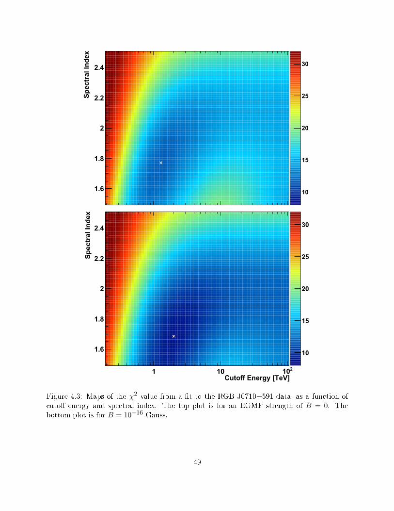
Sp

ectr

al In

dex

1.6

1.8

2

2.2

2.4

10

15

20

25

30

Cutoff Energy [TeV]1 10 210

Sp

ectr

al In

dex

1.6

1.8

2

2.2

2.4

10

15

20

25

30

Figure 4.3: Maps of the χ2 value from a t to the RGB J0710+591 data, as a fun tion of uto energy and spe tral index. The top plot is for an EGMF strength of B = 0. Thebottom plot is for B = 10−16 Gauss.49

EGMF Strength [Gauss]-2010 -1910 -1810 -1710 -1610 -1510 -1410

2 χ

2

4

6

8

10

121 year10 years100 years

years310 years410 years510 years610

Unlimited

90% constraint

95% constraint

Figure 4.4: Test-statisti urves from the intrinsi -spe trum s an, proje ted onto the EGMFeld strength axis, from Huan et al. (2011).Conden e level ∆χ268.3% 190% 2.7295% 3.8499% 6.66Table 4.1: Sele t onden e limits from a χ2(1) distribution.the EGMF strength along the line of sight to RGB J0710+591 at a onden e level of 95%.This limit relaxes by about two orders of magnitude to B > 3 × 10−18 Gauss if the lifetimeis restri ted to the most onservative ase, orresponding to the ∼ 3 years of observations.Due to the un ertainties in the EBL, the assumptions made in onstru ting the model, andthe unknown detailed stru ture of the EGMF, these limits should be thought of as order-of-50

magnitude estimates, rather than rm lower limits. However, the statisti al methods usedto derive them are rigorous and represent the best estimate given the assumptions and thelimited information available.The urves in Figure 4.4 begin to onverge to the unlimited-lifetime ase at a time delayof ∼ 105 years. In order to explain this, it is instru tive to examine the relationship betweenthe angular ut θC and the ut on the lifetime. Equations 4.10 and 4.11 an be ombined,along with a small-angle approximation, to relate these two uts:∆T ≈ L

2c

(

1 − L′

L

)

L′

L

θ2C . (4.13)Assuming the term in bra kets is of order unity when we average over primary gamma-ray energies, we nd for a blazar at a distan e L = 500 Mp that Equation 4.13 gives∆T ≈ 8 × 108θ2C years. The Fermi PSF varies over the energy range of interest from 0.1to a few degrees. Using these values for θC , I nd that the time delay orresponding to thePSF is between 2 × 103 and 4 × 106 years, very mu h in line with the ∼ 105 years impliedby Figure 4.4. If the blazar lifetime is taken to be smaller than this value, then it is more onstraining than the ut due to the PSF and the limit on the eld varies with the lifetime.For longer lifetimes, the xed PSF be omes more onstraining than the lifetime ut, and the urves onverge to the unlimited-lifetime ase.Under the small-angle approximation, θC is proportional to θD by Equation 4.10, andEquation 4.3 demonstrates that θD is proportional to the eld strength B. Combining theseresults with Equation 4.13, we nd that B s ales with √

∆T for time delays below ∼ 105years. Figure 4.5 reinfor es this estimate, demonstrating the expe ted s aling of B with thelifetime and showing the saturation at ∼ 105 years. Sin e the duration of the observationsis about four orders of magnitude below this value, we expe t the limit on the eld to beabout two orders of magnitude smaller than the unlimited-lifetime ase. This is indeed whatis observed.51

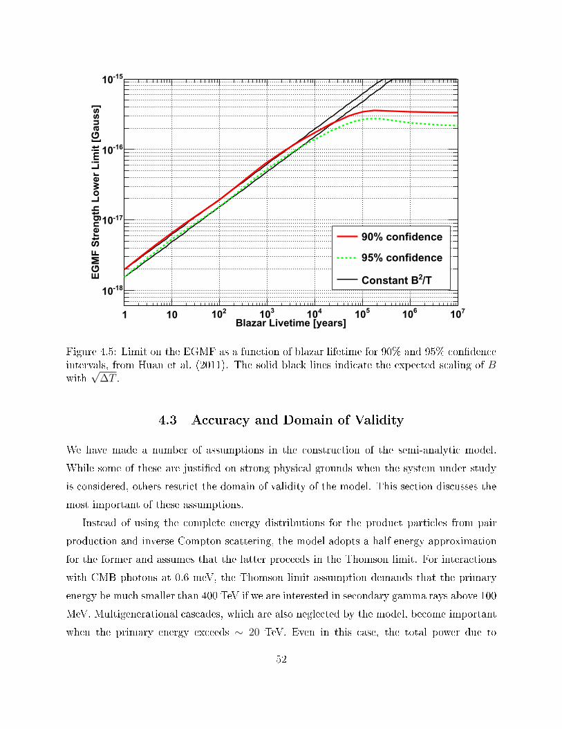
Blazar Livetime [years]1 10 210 310 410 510 610 710

EG

MF

Str

eng

th L

ow

er L

imit

[G

auss

]

-1810

-1710

-1610

-1510

90% confidence

95% confidence

/T2Constant B

Figure 4.5: Limit on the EGMF as a fun tion of blazar lifetime for 90% and 95% onden eintervals, from Huan et al. (2011). The solid bla k lines indi ate the expe ted s aling of Bwith √∆T . 4.3 A ura y and Domain of ValidityWe have made a number of assumptions in the onstru tion of the semi-analyti model.While some of these are justied on strong physi al grounds when the system under studyis onsidered, others restri t the domain of validity of the model. This se tion dis usses themost important of these assumptions.Instead of using the omplete energy distributions for the produ t parti les from pairprodu tion and inverse Compton s attering, the model adopts a half-energy approximationfor the former and assumes that the latter pro eeds in the Thomson limit. For intera tionswith CMB photons at 0.6 meV, the Thomson limit assumption demands that the primaryenergy be mu h smaller than 400 TeV if we are interested in se ondary gamma rays above 100MeV. Multigenerational as ades, whi h are also negle ted by the model, be ome importantwhen the primary energy ex eeds ∼ 20 TeV. Even in this ase, the total power due to52

se ond-generation gamma rays is expe ted to be modest (Tave hio et al., 2010a).The model ignores the ee ts of osmi expansion ex ept in the al ulation of the meanfree path λ(E) of primary gamma rays propagating from the sour e redshift through theEBL. Sin e osmi expansion, energy redshift, and the detailed evolution of the EBL andCMB are ignored, the model is appli able only to nearby sour es at z . 0.2. We have alsoassumed that the EGMF is oherent over the entire traje tory of the ele trons and positrons.As a result, our model is valid provided the EGMF oheren e length is larger than 1 Mp .Another limitation of the model arises from the assumption that gamma rays falling out-side the 68% ontainment radius of the Fermi LAT will not be dete ted. A more appropriateanalysis would a ount fully for the ee ts of the PSF on the extended emission from theblazar. However, this would require a detailed model for the energy-dependent morphologyof the as ade. In order to onstru t this, we would need to sele t sets of upper and lower θC uts and perform an evaluation of Equation 4.9 for ea h set of uts, substantially in reasingthe omputation time.All of the above limitations on the domain of validity of the model argue for a Monte Carlosimulation. This solution ould employ the omplete energy distributions of the fundamentalpro esses, model the EGMF when the oheren e length is smaller than the ooling length ofthe ele trons, a ount for redshift and the expansion of spa e, and follow multiple generationsof the as ade. I explore the development of su h a simulation and its appli ation to Fermiand IACT data in the next two hapters.

53

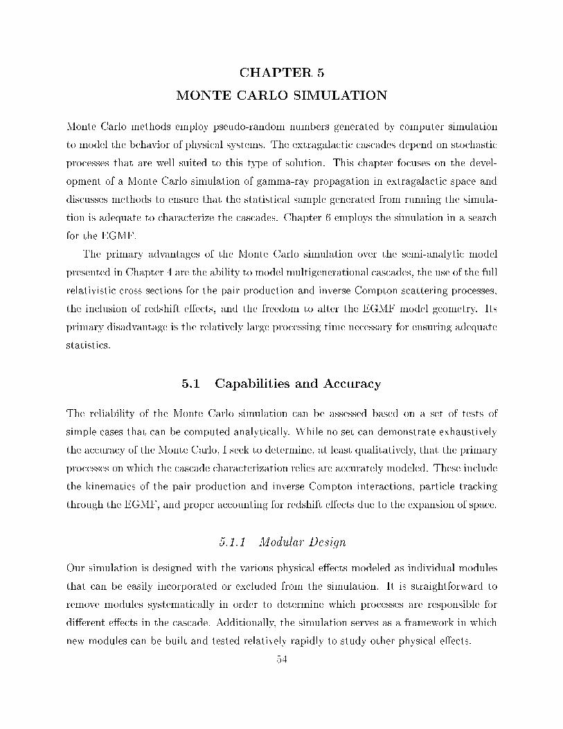
CHAPTER 5MONTE CARLO SIMULATIONMonte Carlo methods employ pseudo-random numbers generated by omputer simulationto model the behavior of physi al systems. The extragala ti as ades depend on sto hasti pro esses that are well suited to this type of solution. This hapter fo uses on the devel-opment of a Monte Carlo simulation of gamma-ray propagation in extragala ti spa e anddis usses methods to ensure that the statisti al sample generated from running the simula-tion is adequate to hara terize the as ades. Chapter 6 employs the simulation in a sear hfor the EGMF.The primary advantages of the Monte Carlo simulation over the semi-analyti modelpresented in Chapter 4 are the ability to model multigenerational as ades, the use of the fullrelativisti ross se tions for the pair produ tion and inverse Compton s attering pro esses,the in lusion of redshift ee ts, and the freedom to alter the EGMF model geometry. Itsprimary disadvantage is the relatively large pro essing time ne essary for ensuring adequatestatisti s. 5.1 Capabilities and A ura yThe reliability of the Monte Carlo simulation an be assessed based on a set of tests ofsimple ases that an be omputed analyti ally. While no set an demonstrate exhaustivelythe a ura y of the Monte Carlo, I seek to determine, at least qualitatively, that the primarypro esses on whi h the as ade hara terization relies are a urately modeled. These in ludethe kinemati s of the pair produ tion and inverse Compton intera tions, parti le tra kingthrough the EGMF, and proper a ounting for redshift ee ts due to the expansion of spa e.5.1.1 Modular DesignOur simulation is designed with the various physi al ee ts modeled as individual modulesthat an be easily in orporated or ex luded from the simulation. It is straightforward toremove modules systemati ally in order to determine whi h pro esses are responsible fordierent ee ts in the as ade. Additionally, the simulation serves as a framework in whi hnew modules an be built and tested relatively rapidly to study other physi al ee ts.54

The main assumptions impli it in the Monte Carlo ode are as follows:• Both ontinuous and dis rete pro esses an be modeled. Continuous pro esses alterthe dynami properties of the tra ked parti les as they propagate, while dis rete inter-a tions involving ba kground parti les o ur at spe i points in spa etime.• We assume that the ba kground parti le populations are isotropi and homogeneous.Any type of ba kground parti les an be in luded; they need not be photons.• Intera tions o ur between two parti les but an produ e an arbitrary number of se -ondary parti les. The primary parti le an survive the intera tion, or it an be de-stroyed.The parti les of the as ade are tra ked via omoving oordinates in a fully three-dimensional expanding spa e. Stepper routines, des ribed in detail in Se tion 5.1.3, followthe evolution of the dynami properties of ea h as ade parti le with a predetermined levelof a ura y. Ea h ontinuous pro ess spe ies its ontribution to the rate of hange of mo-mentum for the tra ked parti le, while ea h dis rete pro ess requires a table of the meanfree path of the tra ked parti le as a fun tion of its energy and redshift. The onstru tion ofthe tables pro eeds by evaluating Equations 2.25 and 2.26. These tables an be omputedeither at simulation run-time or in advan e, although the latter ase saves a great deal ofpro essing time if the simulation is run repeatedly.5.1.2 Parti le Kinemati sOur simulation employs the full relativisti ross se tions for pair produ tion and inverseCompton s attering as given by Equations 2.8 and 2.16, respe tively. The ode samplesthe target photon energies from the mean free path tables and other kinemati variablesfrom the results of Protheroe (1986) for pair produ tion or Jones (1968) and Blumenthal& Gould (1970) for inverse Compton s attering. The properties of the produ t parti lesfrom the intera tion are then determined based on the relativisti kinemati s as dis ussedin Se tions 2.2.1 and 2.3.1. In this se tion, I summarize the kinemati s of both relevantintera tions and demonstrate the ode's ability to reprodu e simple results. Although I makesimplifying assumptions in determining the analyti results, of ourse the ode employs thegeneral solution in ea h ase. 55

Fraction of Parent Energy0 0.1 0.2 0.3 0.4 0.5 0.6 0.7 0.8 0.9 1

No

rmal

ized

Co

un

ts

0

0.5

1

1.5

2

2.5

3

3.5

4

10 TeV25 TeV

100 TeVAnalytic

Figure 5.1: Distribution of produ t ele tron and positron energies from gamma rays under-going pair produ tion on a 30-meV monoenergeti ba kground. Primary gamma rays areinje ted at 10, 25, and 100 TeV. The histograms are from the Monte Carlo simulation, whilethe gray lines are from the analyti al ulation of Zdziarski (1988).Zdziarski (1988) has omputed the distribution of produ t photon energies for pair pro-du tion intera tions on an isotropi ba kground with an arbitrary spe trum. Figure 5.1shows the simulated results from our ode when the ba kground onsists of monoenergeti photons of energy ǫ = 30 meV. This energy is at the high-energy edge of the infrared peakin the EBL. Analyti predi tions from Zdziarski (1988) also appear in the gure. The ode learly mat hes the predi ted values very well. Figure 5.1 highlights the inadequa y of thehalf-energy approximation when the gamma-ray energy is large; as one of the produ t leptonsa quires most of the primary's energy, the distribution of parti le energies in the as ademay hange signi antly. 56

q0 0.1 0.2 0.3 0.4 0.5 0.6 0.7 0.8 0.9 1

No

rmal

ized

Co

un

ts

0

2

4

6

8

10

12

14

16

18

20

10 TeV25 TeV

100 TeVAnalytic

Figure 5.2: Distribution of q for pair produ tion targets when the ba kground is monoener-geti at 30 meV, along with analyti predi tions.Due to relativisti and geometri ee ts, the distribution of dire tions of target photonsthat intera t is not isotropi , despite the isotropi nature of the ba kground population.By inspe tion of Equation 2.25, it is lear that the appropriate distribution is σγγ(q)/q3.When q is sampled from this distribution, Equation 2.2 determines the angle of the targetphoton. Figure 5.2 demonstrates that the sampling of q from the ode1 is in line with ourexpe tations from Equation 2.25.The nal kinemati variable that must be sampled for pair produ tion is the angle ofemission of the ele tron with respe t to the gamma ray's dire tion. This angle is labeled asα′ in Figure 2.3 and its distribution is given by Jau h & Rohrli h (1976). In the enter of1. In pra ti e, the ode samples from the distribution in terms of the Mandelstam variable s; however,this is a matter of semanti s. 57

Target Energy [eV]-310 -210 -110 1 10

]-1

pc

-1In

tera

ctio

n R

ate

[eV

-1110

-1010

-910

-810

-710

-610

-510

-410

-310

10 TeV

100 TeV

Analytic

Figure 5.3: Distribution of target energies for pair produ tion on the EBL of Fran es hiniet al. (2008), at a redshift of z = 0.1. The bla k urves indi ate the expe ted distributionsof target energies from Equation 2.25.momentum frame, the azimuthal angle of the outgoing ele tron is sampled from a uniformdistribution. This pro edure is ne essary be ause the physi s in the enter of momentumframe exhibits azimuthal symmetry with respe t to the dire tion of the primary photon, andnot with respe t to the boost dire tion, making the azimuthal angle important in the returnboost. The ode al ulates the momenta of the leptons in the enter of momentum framea ording to the dis ussion in Se tion 2.2.1. A boost ba k into the lab frame then produ esthe traje tories of the ele tron and positron, whi h are added to the tra ked parti les in the as ade.Figure 5.3 displays the distributions of target energies for pair produ tion intera tions onthe full EBL as given by Fran es hini et al. (2008), along with the expe ted distribution of58

Interaction Distance [pc]510 610 710 810 910

No

rmal

ized

Co

un

ts

-1310

-1210

-1110

-1010

-910

-810

-710

-610

10 TeV

100 TeV

Analytic

Figure 5.4: Distribution of intera tion lengths for pair produ tion on the EBL of Fran es- hini et al. (2008), at a redshift of z = 0.1. The bla k urves indi ate the evaluation ofEquation 2.25.target energies from Equation 2.25. In the gure, the primary gamma rays are inje ted at aredshift of z = 0.1. The distributions of their intera tion lengths appear in Figure 5.4, alongwith the predi tions from integrating Equation 2.25, again showing good agreement. The uto in the distribution of 10-TeV gamma-ray intera tion lengths at 420 Mp is expe tedbe ause this is the distan e to a sour e at z = 0.1 and the gamma rays are not tra ked beyonda distan e equal to the omoving distan e between the sour e and the observer. That is,10-TeV gamma rays that survive the propagation from the sour e to Earth are not in ludedin the histograms in Figure 5.4. Obviously no su h uto is manifest in the distribution of100-TeV gamma rays be ause their mean free path is mu h smaller and all of them intera t.We adopt a similar approa h in testing the a ura y of inverse Compton s attering in59

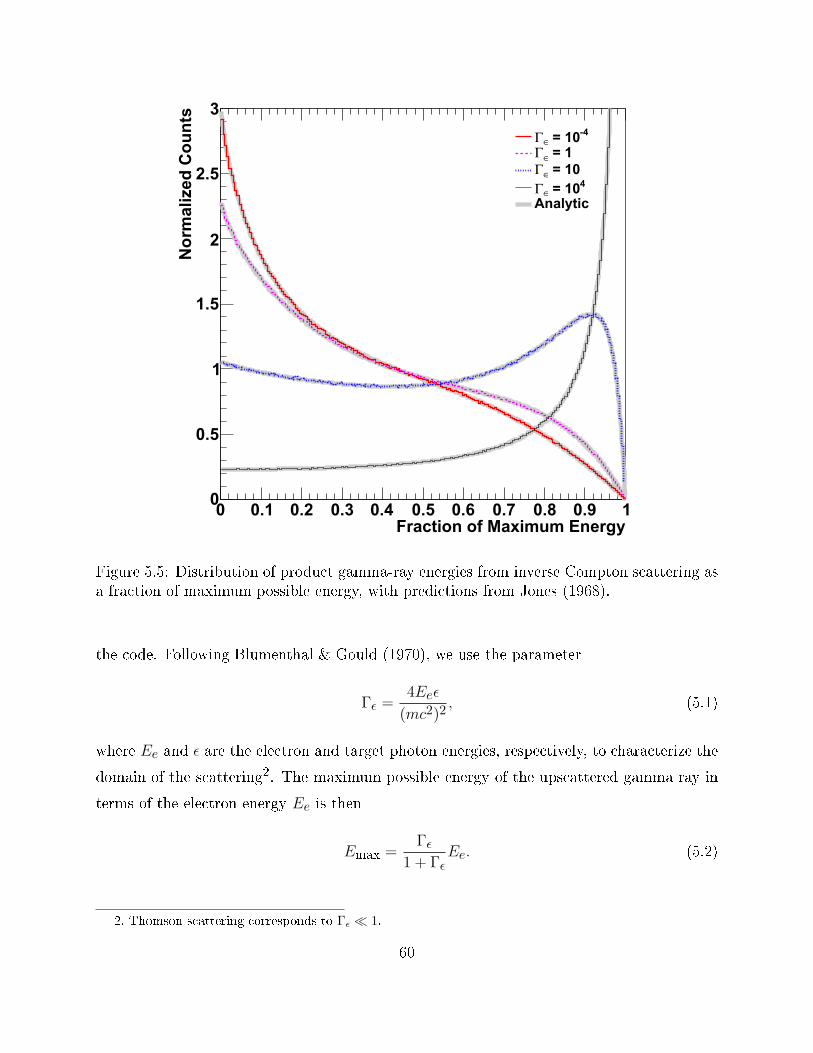
Fraction of Maximum Energy0 0.1 0.2 0.3 0.4 0.5 0.6 0.7 0.8 0.9 1

No

rmal

ized

Co

un

ts

0

0.5

1

1.5

2

2.5

3-4 = 10∈Γ

= 1∈Γ = 10∈Γ

4 = 10∈ΓAnalytic

Figure 5.5: Distribution of produ t gamma-ray energies from inverse Compton s attering asa fra tion of maximum possible energy, with predi tions from Jones (1968).the ode. Following Blumenthal & Gould (1970), we use the parameterΓǫ =

4Eeǫ

(mc2)2, (5.1)where Ee and ǫ are the ele tron and target photon energies, respe tively, to hara terize thedomain of the s attering2. The maximum possible energy of the ups attered gamma ray interms of the ele tron energy Ee is then

Emax =Γǫ

1 + ΓǫEe. (5.2)2. Thomson s attering orresponds to Γǫ ≪ 1. 60

x0 0.1 0.2 0.3 0.4 0.5 0.6 0.7 0.8 0.9 1

No

rmal

ized

Co

un

ts

0

0.2

0.4

0.6

0.8

1

1.2

1.4

1.6

1.8

2 -4 = 10∈Γ = 0.1∈Γ = 1∈Γ = 10∈Γ

4 = 10∈ΓAnalytic

Figure 5.6: Distribution of x from inverse Compton s attering.Jones (1968) gives the distribution of Emax as a fun tion of Γǫ, whi h appears alongwith the distributions from the ode in Figure 5.5, again showing good agreement betweenthe ode and the analyti al ulation. In the gure, ele trons at 10 TeV intera t with anappropriate monoenergeti ba kground to fulll the requested Γǫ, with the ase Γǫ = 1representing intera tions with the peak of the CMB.The parameter x from Equation 2.13 is bounded by the values x− and x+ from Equa-tion 2.30. We onstru t a value x bounded by 0 and 1 via the transformationx =

x− x−x+ − x−

. (5.3)Figure 5.6 shows the distribution of x from Equation 2.13 for the same simulation runs usedto onstru t Figure 5.5. This distribution is sampled from xσeγ(x), a pro edure inspired by61

inspe tion of Equation 2.24. The a ura y of the distributions in x apparent in Figure 5.6implies via Equation 2.13 that the ode samples the proper distribution of angles betweenthe ele tron and target photon.In a manner similar to its treatment of the pair produ tion intera tion, after the energyand angle of the target photon are sampled, the ode performs a boost to the enter of massframe in whi h the ele tron is at rest, as shown in Figure 2.6(b). The dee tion angle ofthe photon is then sampled from Equation 2.14, the ode omputes the kinemati s of theintera tion as des ribed in Se tion 2.3.1, and the resulting parti les are boosted ba k to thelab frame. In ontrast to the ase of pair produ tion, be ause the ele tron is initially at restin the enter of mass frame, azimuthal symmetry exists along the boost dire tion, so theazimuthal angle is unae ted by the boost and an be omputed upon the return boost tothe lab frame.The distribution of target energies for a 10-TeV ele tron inje ted at a distan e of 400 kp appears in Figure 5.7, together with the expe ted distribution spe ied by the integrand ofthe integral over the ba kground energy from Equation 2.24. Sin e the mean free path of theele trons is about 1 kp , well below the gala ti s ale, the ele trons are virtually guaranteedto intera t. It is lear in the gure that the distributions produ ed by the ode mat h ourexpe tations very well for energies above 4 × 10−6 eV. Below this energy, the small CMBdensity ontributes less than 0.01% of the intera tion rate above 4× 10−6 eV, so we ele t totrun ate the CMB distribution at this energy. Furthermore, Figure 5.8 demonstrates thatthe distribution of intera tion lengths for the 10-TeV ele trons is onsistent with our estimateof 1 kp . The analyti urve in Figure 5.8 is a de aying exponential with a hara teristi length s ale determined by integration of the analyti urve in Figure 5.7.One important point evident in Figure 5.7 is that the EBL plays a role in the ele trons'intera tions. For 10-TeV ele trons, intera tions with the peak of the CMB o ur at a fa torΓǫ ≈ 1. In this ase, Equation 5.1 informs us that the maximum fra tion fmax of theele tron's energy that an be lost is fmax = 1/2, and a ording to Figure 5.5 the ele tron islikely to lose only a small fra tion of this maximum. In ontrast, for intera tions with theinfrared peak of the EBL, o urring at Γǫ ≈ 10, the ele trons are likely to lose a large fra tionof the maximum fra tion fmax = 10/11. Despite their rarity, intera tions with the EBL antherefore limit the number of lower-energy gamma rays in the as ade, while at the sametime enhan ing the ux of higher-energy gamma rays. As I des ribe in detail in Se tion 5.3,62

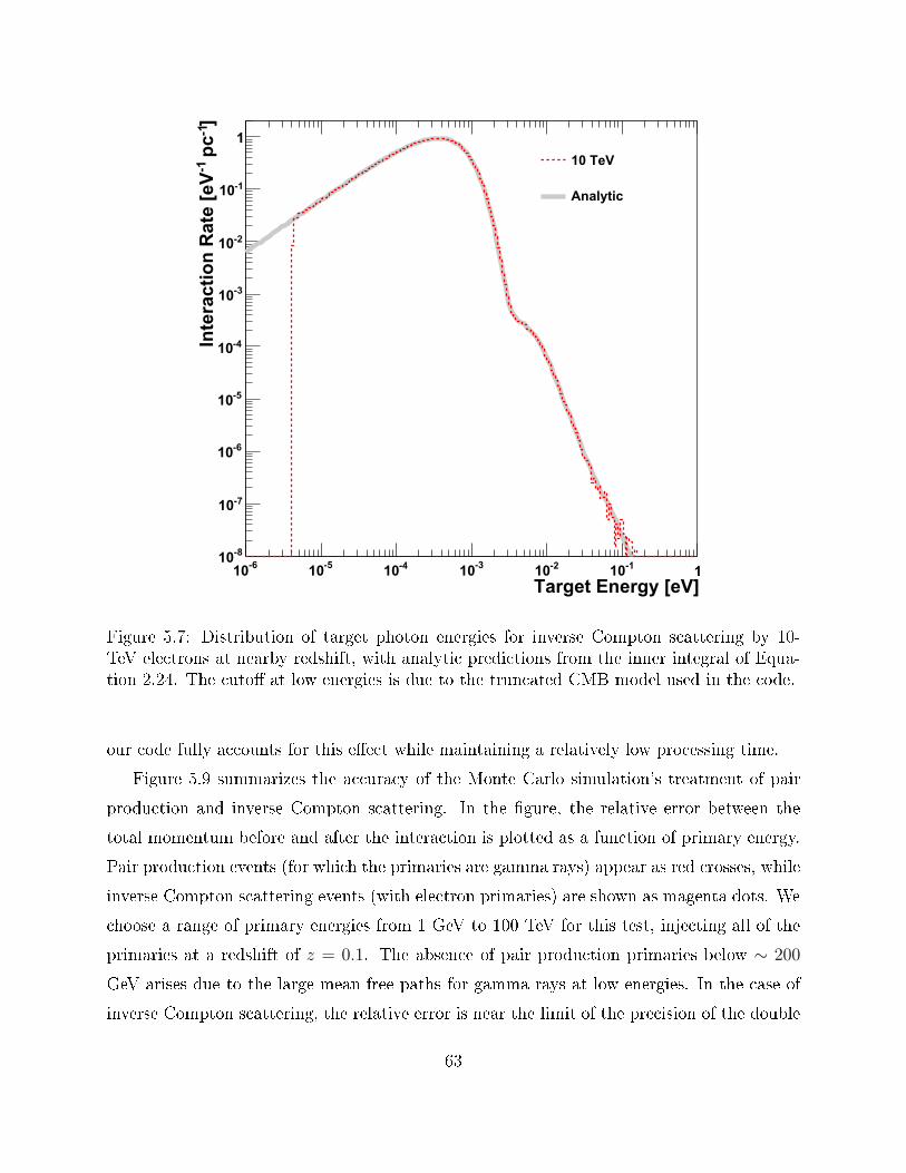
Target Energy [eV]-610 -510 -410 -310 -210 -110 1

]-1

pc

-1In

tera

ctio

n R

ate

[eV

-810

-710

-610

-510

-410

-310

-210

-110

1

10 TeV

Analytic

Figure 5.7: Distribution of target photon energies for inverse Compton s attering by 10-TeV ele trons at nearby redshift, with analyti predi tions from the inner integral of Equa-tion 2.24. The uto at low energies is due to the trun ated CMB model used in the ode.our ode fully a ounts for this ee t while maintaining a relatively low pro essing time.Figure 5.9 summarizes the a ura y of the Monte Carlo simulation's treatment of pairprodu tion and inverse Compton s attering. In the gure, the relative error between thetotal momentum before and after the intera tion is plotted as a fun tion of primary energy.Pair produ tion events (for whi h the primaries are gamma rays) appear as red rosses, whileinverse Compton s attering events (with ele tron primaries) are shown as magenta dots. We hoose a range of primary energies from 1 GeV to 100 TeV for this test, inje ting all of theprimaries at a redshift of z = 0.1. The absen e of pair produ tion primaries below ∼ 200GeV arises due to the large mean free paths for gamma rays at low energies. In the ase ofinverse Compton s attering, the relative error is near the limit of the pre ision of the double63

Interaction Distance [pc]1 10 210 310 410 510

No

rmal

ized

Co

un

ts

-910

-810

-710

-610

-510

-410

-310

-210

10 TeV

Analytic

Figure 5.8: Distribution of 10-TeV ele trons' intera tion lengths for inverse Compton s at-tering.data type of ∼ 10−16, and this auses the stru ture observed in the gure. The relativeerrors below this value are due to a idental an ellations in ma hine rounding. For pairprodu tion, the relative error is somewhat higher but still less than 10−10, whi h is morethan a eptable.The kinemati s of the as ade involves large boosts along or nearly along the dire tionof the primary parti le. For this reason, it is important to he k onservation of momentumperpendi ular to the dire tion of the primary, in addition to total onservation of energy.Figure 5.10 shows that the ode onserves this transverse momentum at an a ura y of betterthan 10−6.64

Primary Energy [eV]1010 1110 1210 1310 1410

Rel

ativ

e E

rro

r

-2810

-2610

-2410

-2210

-2010

-1810

-1610

-1410

-1210

-1010

-810

Pair Production

Inverse Compton

Figure 5.9: A ura y of total momentum onservation for both pair produ tion (red rosses)and inverse Compton (magenta dots) intera tions.5.1.3 Parti le Tra kingThe Monte Carlo simulation implements parti le tra king by numeri ally integrating theequations of motion for the individual parti les in an expanding three-dimensional spa e.We employ omoving oordinates in the parti le tra king, for whi h physi al distan es anbe determined by multiplying the omoving separation by the s ale fa tor at a given red-shift (Kolb & Turner, 1990). This makes the equations of motion more ompli ated to solvebut is on eptually simpler.A detailed derivation of the equations of motion appears in Appendix A. For a parti lemoving in a spatially uniform magneti eld with evolution given by Equation 1.1, the65

Primary Energy [eV]1010 1110 1210 1310 1410

Rel

ativ

e E

rro

r

-1210

-1110

-1010

-910

-810

-710

-610

Pair Production

Inverse Compton

Figure 5.10: A ura y of momentum onservation transverse to the dire tion of the primary,for pair produ tion (red rosses) and inverse Compton (magenta dots) intera tions. Thetransition in the inverse Compton error distribution at ∼ 5 GeV is due to the approximationof the ele tron speed β ≈ 1 − 1/2γ2.equations of motion be omed

dt~p = −H(z)~p+

q

mγ~p× ~B(z), (5.4)where q is the parti le's harge and the se ond term on the right hand side vanishes forgamma rays be ause they do not ouple to the magneti eld, at least to rst order.In the ode, we implement a fourth-order Runge-Kutta method, referred to as a stepperin the rest of this se tion, to solve the dierential equations of motion. The order of the step-per indi ates the highest power of the step size in the expansion of the equations of motion,and the fourth-order Runge-Kutta method is parti ularly attra tive due to the serendipitous66

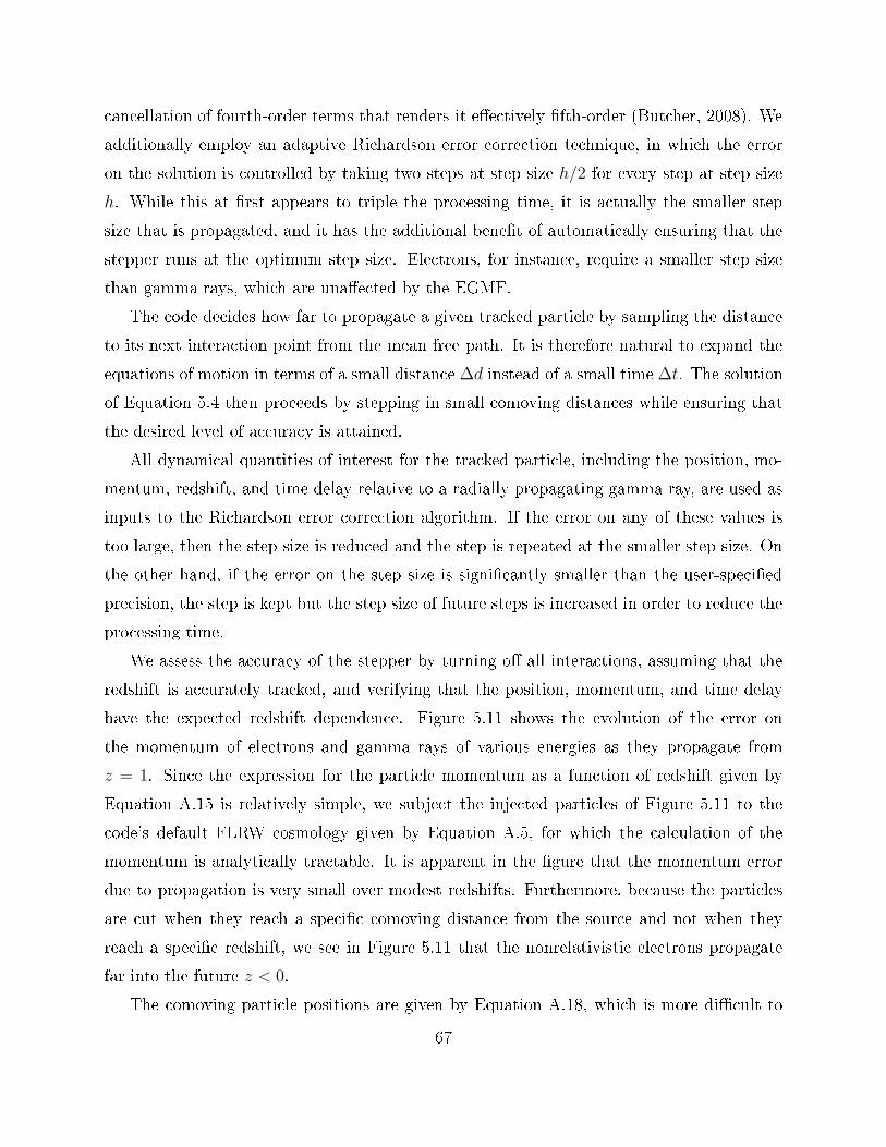
an ellation of fourth-order terms that renders it ee tively fth-order (But her, 2008). Weadditionally employ an adaptive Ri hardson error orre tion te hnique, in whi h the erroron the solution is ontrolled by taking two steps at step size h/2 for every step at step sizeh. While this at rst appears to triple the pro essing time, it is a tually the smaller stepsize that is propagated, and it has the additional benet of automati ally ensuring that thestepper runs at the optimum step size. Ele trons, for instan e, require a smaller step sizethan gamma rays, whi h are unae ted by the EGMF.The ode de ides how far to propagate a given tra ked parti le by sampling the distan eto its next intera tion point from the mean free path. It is therefore natural to expand theequations of motion in terms of a small distan e ∆d instead of a small time ∆t. The solutionof Equation 5.4 then pro eeds by stepping in small omoving distan es while ensuring thatthe desired level of a ura y is attained.All dynami al quantities of interest for the tra ked parti le, in luding the position, mo-mentum, redshift, and time delay relative to a radially propagating gamma ray, are used asinputs to the Ri hardson error orre tion algorithm. If the error on any of these values istoo large, then the step size is redu ed and the step is repeated at the smaller step size. Onthe other hand, if the error on the step size is signi antly smaller than the user-spe iedpre ision, the step is kept but the step size of future steps is in reased in order to redu e thepro essing time.We assess the a ura y of the stepper by turning o all intera tions, assuming that theredshift is a urately tra ked, and verifying that the position, momentum, and time delayhave the expe ted redshift dependen e. Figure 5.11 shows the evolution of the error onthe momentum of ele trons and gamma rays of various energies as they propagate fromz = 1. Sin e the expression for the parti le momentum as a fun tion of redshift given byEquation A.15 is relatively simple, we subje t the inje ted parti les of Figure 5.11 to the ode's default FLRW osmology given by Equation A.5, for whi h the al ulation of themomentum is analyti ally tra table. It is apparent in the gure that the momentum errordue to propagation is very small over modest redshifts. Furthermore, be ause the parti lesare ut when they rea h a spe i omoving distan e from the sour e and not when theyrea h a spe i redshift, we see in Figure 5.11 that the nonrelativisti ele trons propagatefar into the future z < 0.The omoving parti le positions are given by Equation A.18, whi h is more di ult to67

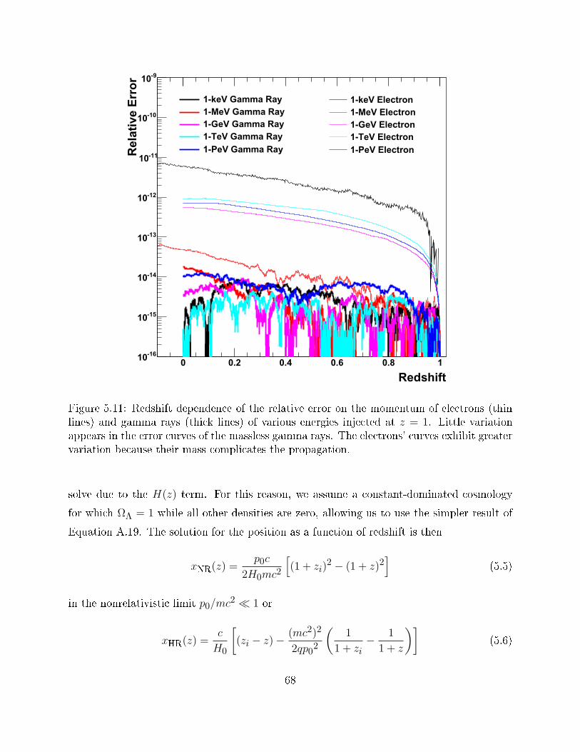
Redshift0 0.2 0.4 0.6 0.8 1

Rel

ativ

e E

rro

r

-1610

-1510

-1410

-1310

-1210

-1110

-1010

-910

1-keV Electron1-MeV Electron1-GeV Electron1-TeV Electron1-PeV Electron

1-keV Gamma Ray1-MeV Gamma Ray1-GeV Gamma Ray1-TeV Gamma Ray1-PeV Gamma Ray

Figure 5.11: Redshift dependen e of the relative error on the momentum of ele trons (thinlines) and gamma rays (thi k lines) of various energies inje ted at z = 1. Little variationappears in the error urves of the massless gamma rays. The ele trons' urves exhibit greatervariation be ause their mass ompli ates the propagation.solve due to the H(z) term. For this reason, we assume a onstant-dominated osmologyfor whi h ΩΛ = 1 while all other densities are zero, allowing us to use the simpler result ofEquation A.19. The solution for the position as a fun tion of redshift is thenxNR(z) =

p0c

2H0mc2

[

(1 + zi)2 − (1 + z)2

] (5.5)in the nonrelativisti limit p0/mc2 ≪ 1 orxHR(z) =

c

H0

[

(zi − z) − (mc2)2

2qp02

(

1

1 + zi− 1

1 + z

)] (5.6)68

Redshift-0.2 0 0.2 0.4 0.6 0.8 1

Po

siti

on

[M

pc]

210

310

410

1-keV Electron100-keV Electron1-MeV ElectronGamma Rays

CDMΛ100-keV Electron in Nonrelativistic CalculationsHighly Relativistic Calculation

Figure 5.12: Comoving distan e as a fun tion of redshift for parti les of various energies ina onstant-dominated osmology. A 100-keV ele tron in a ΛCDM osmology is also shownfor omparison.in the highly relativisti limit p0/mc2 ≫ 1. In these equations, the momentum of the par-ti le at the present day is p0, and zi is the initial redshift of the parti le. Figure 5.12 showsthe redshift evolution of the omoving distan e for various parti les. At 1 keV, the predi -tions from the nonrelativisti approximation of Equation 5.5 agree well with the propagatedparti les in the ode, while at 100 keV there is evident divergen e. Also as expe ted, thepropagation of gamma rays mat hes the highly relativisti predi tion of Equation 5.6, andthe marginally relativisti ele trons at 1 MeV follow nearly the same evolution as the gammarays.Figure 5.13 shows the error on the time delay of ele trons with kineti energies from 5keV to 28 GeV propagating a distan e of 4283 Mp . The nonrelativisti approximation from69

]2Momentum [mc-310 -210 -110 1 10 210 310 410 510

Tim

e D

elay

[M

yr]

-610

-510

-410

-310

-210

-110

1

10

210

310

410

510

Electrons

Nonrelativistic

CDMΛElectrons in

Figure 5.13: Time delay of ele trons of various energies propagating from z = 1 to z = 0,with respe t to the propagation time of a gamma ray.Equation A.31 mat hes the simulation results for low energies.5.1.4 Energy LossesParti les ontinuously lose energy due to redshift during their propagation. To fa ilitate omputation, the ode an also enter a mode of propagation in whi h the intera tions ofele trons and positrons with the CMB are modeled as a ontinuous energy loss pro ess.This mode is triggered in the extreme Thomson limit when it is impossible for ele tronsto produ e observable se ondary gamma rays from CMB intera tions but the produ tion ofobservable se ondaries from the EBL is still possible. I dis uss this mode in greater detailin Se tion 5.3.1. In both ases, energy losses ae t the mean free path of the parti le ina ontinuous manner throughout its propagation, and simple sampling of the intera tion70

X [Mpc]-0.6 -0.4 -0.2 0 0.2 0.4 0.6

Y [

Mp

c]

-0.6

-0.4

-0.2

0

0.2

0.4

0.6

Gauss-16B = 10

Gauss, scaled by 3-15B = 10

Gauss, scaled by 10-14B = 10

Figure 5.14: Paths of 100-GeV ele trons in omoving oordinates. A onstant, uniform eldexists perpendi ular to the ir ular traje tories. The radii for the stronger eld strengthsare s aled by 3 and 10 to better t on the plot. Dashed lines ending in lled ir les indi atethe expe ted radius from Equation 5.4.length from the mean free path is no longer valid.Our solution is to sample the intera tion length not from the mean free path of the parti leat its initial energy, but rather from the minimum mean free path along its entire potentialtraje tory. After propagating the parti le this sampled distan e, we a ept the intera tionwith a probability λ0/λ(L+L1), where λ0 is the minimum mean free path, λ(L) is the meanfree path as a fun tion of the length along the traje tory, and the parti le is propagatingfrom distan e L1 to L. The justi ation for this pro edure appears in Appendix B.71

5.1.5 Magneti FieldsIn Eu lidean spa e, in the presen e of a magneti eld, an ele tron of onstant energy followsa spiral traje tory with Larmor radius given by Equation 2.31. In an expanding spa e, theele tron's traje tory remains spiral with the same radius in omoving oordinates. This isapparent from Equation 5.4 and an be thought of as follows: the eld strength evolvesas (1 + z)2 a ording to Equation 1.1, while the ele tron's momentum evolves as (1 + z).Equation 2.31 then tells us that the Larmor radius in real oordinates evolves as (1 + z)−1,at the same rate as the expansion, implying that the radius of the spiral traje tory in omoving oordinates does not hange. Figure 5.14 demonstrates that the ode reprodu esour expe tations from these al ulations.Stronger magneti eld strengths ause greater dee tions of the ele trons and positrons,resulting in a smaller required step size to maintain the desired level of a ura y. Thepro essing time due to the smaller step size for EGMF strengths above ∼ 10−15 Gauss anbe ome prohibitively expensive. To ombat this, we implement a ut that removes ele tronson e their traje tories have been dee ted by an angle of more than π/2 from the dire tion ofthe primary gamma ray. Su h ele trons are equally likely to produ e a se ondary gamma rayin any dire tion, so their ontribution to the as ade is indistinguishable from the isotropi diuse gamma-ray ux and an be safely ignored.5.1.6 Multigenerational Cas adesThe presen e of signi ant gamma-ray ux above 10 TeV in the intrinsi spe trum an leadto multigenerational as ades, in whi h the se ondary gamma rays an themselves undergopair produ tion intera tions and produ e ups attering ele trons and positrons. These multi-generational as ades are ignored in the semi-analyti model des ribed in Chapter 4. Whileit is possible to in lude the ee ts of multigenerational as ades in ertain models, su h asthe model of Ahlers (2011), su h models have their own limitations that a Monte Carlo sim-ulation an straightforwardly over ome3. Figure 5.15 demonstrates the ability of the ode tomodel multigenerational as ades. It is lear that at least se ond-generation gamma rays anbe important in the 1-GeV to 10-GeV energy range if the intrinsi spe trum has substantialux at 20 TeV.3. For instan e, Ahlers (2011) makes the assumption that the gamma-ray sour e emits isotropi ally.72

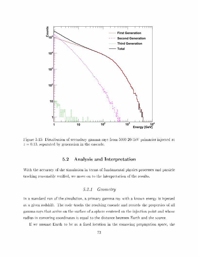
Energy [GeV]1 10 210 310 410

Co

un

ts

1

10

210

310

410

510First Generation

Second Generation

Third Generation

Total

Figure 5.15: Distribution of se ondary gamma rays from 5000 20-TeV primaries inje ted atz = 0.13, separated by generation in the as ade.5.2 Analysis and InterpretationWith the a ura y of the simulation in terms of fundamental physi s pro esses and parti letra king reasonably veried, we move on to the interpretation of the results.5.2.1 GeometryIn a standard run of the simulation, a primary gamma ray with a known energy is inje tedat a given redshift. The ode tra ks the resulting as ade and re ords the properties of allgamma rays that arrive on the surfa e of a sphere entered on the inje tion point and whoseradius in omoving oordinates is equal to the distan e between Earth and the sour e.If we assume Earth to be at a xed lo ation in the omoving propagation spa e, the73

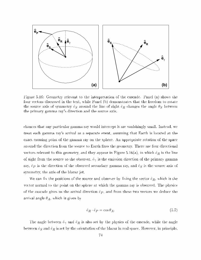
Pe

Re

Seγe

(a)

ReSe

γe

(b)Figure 5.16: Geometry relevant to the interpretation of the as ade. Panel (a) shows thefour ve tors dis ussed in the text, while Panel (b) demonstrates that the freedom to rotatethe sour e axis of symmetry eS around the line of sight eR hanges the angle θS betweenthe primary gamma ray's dire tion and the sour e axis. han es that any parti ular gamma ray would inter ept it are vanishingly small. Instead, wetreat ea h gamma ray's arrival as a separate event, assuming that Earth is lo ated at theexa t rossing point of the gamma ray on the sphere. An appropriate rotation of the spa earound the dire tion from the sour e to Earth xes the geometry. There are four dire tionalve tors relevant to this geometry, and they appear in Figure 5.16(a), in whi h eR is the lineof sight from the sour e to the observer, eγ is the emission dire tion of the primary gammaray, eP is the dire tion of the observed se ondary gamma ray, and eS is the sour e axis ofsymmetry, the axis of the blazar jet.We an x the positions of the sour e and observer by xing the ve tor eR, whi h is theve tor normal to the point on the sphere at whi h the gamma ray is observed. The physi sof the as ade gives us the arrival dire tion eP , and from these two ve tors we dedu e thearrival angle θA, whi h is given byeR · eP = cos θA. (5.7)The angle between eγ and eR is also set by the physi s of the as ade, while the anglebetween eS and eR is set by the orientation of the blazar in real spa e. However, in prin iple,74

any angle θS between the jet axis eS and the momentum of the primary eγ is admissible,so we have the freedom to rotate eS around eR, as shown in Figure 5.16(b). This operationobviously hanges the value of θS and onsequently hanges the weight from the intrinsi blazar spe trum as given by Equation 3.1. Denoting the azimuthal angle by whi h the ve toreS is rotated out of the eγ-eR plane as φR, we see from straightforward geometry that

cos θS = cos θ cos θV + sin θ sin θV cosφR, (5.8)where θV is the viewing angle of the blazar (the angle between eR and eS), and θ is thedee tion angle of the se ondary gamma ray relative to the primary (the angle between eRand eγ). This geometry is of ourse important only for a blazar whose jet axis is not alignedwith the line of sight. In this general ase, we sample φR uniformly on [−π, π) for ea hse ondary gamma ray to onstru t the observed ux. We then employ Equation 3.1 to getthe weight fa tor for the gamma ray.5.2.2 The Cas ade FluxThe omputation of the ux from the as ade pro eeds in two stages. In the rst, these ondary photons are olle ted and weighted by the ux from Equation 3.1 based on theenergy of the primary gamma ray that reated their as ade and the randomly sampled angleφR as dis ussed in the previous se tion. The weights are normalized su h that the total ux

Ftot ≡ F0dN

dΩdtdE(5.9)fullls the equation

∫

dΩ

∫

dt

∫

dEFtot = 1, (5.10)where Ω is the solid angle, E is the energy, and t is the time of arrival. The variable t an bewritten in terms of the time delay ∆T a rued during propagation and the time of primaryemission at the sour e τ ast = ∆T + (1 + z)τ, (5.11)in whi h the redshift of the sour e appears be ause time dieren es at the sour e are mag-nied by the expansion of spa e during the time interval. Any generi time prole for the75

-1410

-1310

-1210

-1110

-1010

RA Offset [degrees]-2 -1.5 -1 -0.5 0 0.5 1 1.5 2

DE

C O

ffse

t [d

egre

es]

-2

-1.5

-1

-0.5

0

0.5

1

1.5

2

Figure 5.17: Simulated sky map in units of gamma rays m−2 s−1 sr−1 for the as adeemission from a blazar with an intrinsi spe tral index 1.5, uto energy 10 TeV, redshift 0.13,and misalignment angle of 5, with an EGMF strength of 10−15 Gauss. The misalignmentangle is hosen to lie along the right as ension (RA) axis, in the negative dire tion, as isevident in the map.sour e an be spe ied, though the analyses presented in this work assume a onstant uxindependent of time. There is also an option to in lude an instrument PSF at this stage,whi h allows us to investigate instrumental ee ts.The se ond stage of the analysis involves generating distributions subje t to ertain uts.In general, the distributions to be onstru ted depend on the spe i physi s goals of theanalysis. For example, the spe trum of gamma rays within a ertain angular separationfrom the sour e may be of interest, or a sky map of the as ade within a ertain energyband may be onstru ted. These distributions are weighted based on the weights al ulatedin the rst stage. A sample sky map of the as ade onstru ted from the simulation of ablazar with a misalignment angle of θV = 5 appears in Figure 5.17. I plot the spe trumof the various ux omponents in Figure 5.18. The dire t emission in Figure 5.18 is the76

Energy [eV]910 1010 1110 1210 1310 1410

]-2

s-2

dN

/dE

[er

g c

m2

E

-1210

-1110

Intrinsic

Direct

Cascade

Total

Figure 5.18: Simulated spe trum of the as ade emission from Figure 5.17. The energy lostdue to attenuation of the intrinsi spe trum produ es the ux in the as ade, highlighting therole of the photon ba kgrounds in onverting TeV-s ale gamma rays into GeV-s ale gammarays.remaining pointlike ux from the blazar after the intrinsi emission has intera ted with theEBL. The as ade emission in the gure results from the repro essed intrinsi ux thatforms the extended halo of Figure 5.17. Observations of the total ux, whi h is the sum ofthe as ade and dire t, may reveal information about the as ade if the eld is su ientlystrong. If the eld is weak, then for this parti ular intrinsi spe trum the observed total uxin the the GeV energy band will be dominated by the as ade gamma rays.77

Inje tion Energy No Transition Energy 300-GeV Transition Energy1 TeV 156 s 1.85 s10 TeV 351 s 61.4 s100 TeV 5050 s 572 sTable 5.1: Pro essing times with and without a transition energy of 300 GeV for as ades ofvarious energies. The energy ut is 8.66 GeV.5.3 Adequate Statisti sOne must nd a balan e between the pro essing time for a set of simulations and the a ura yresulting from that set. We have devised a generi pro edure to ensure the a ura y of ourresults. In this se tion, I present the spe i realization of this pro edure used in the analysesof Chapter 6, but the details su h as the energy binning and the desired a ura y an easilybe modied for a parti ular appli ation.We restri t our attention in this se tion and throughout the following hapter to gammarays with energies greater than 866 MeV, whi h we dene to be observable. This energyis sele ted be ause it is the low edge of an energy bin entered at 1 GeV when the energyis binned with eight bins per de ade and spa ed evenly in logarithmi spa e. I present thereasoning behind this sele tion in Se tion 5.3.2.5.3.1 The Transition EnergyAs shown in Se tion 2.4.2, the dominant intera tion hannel for the inverse Compton pro essis via intera tions with the CMB. As the ele trons ool, the ups attered gamma rays tend tobe produ ed with smaller energies until the maximum possible energy from Equation 2.18 isless than our observable energy of 866 MeV. At this point, CMB intera tions are irrelevant,but it is still possible for EBL intera tions to produ e observable se ondaries. Terminatingthe ele tron tra king at this stage ould therefore lead to an ina urately low predi tion forthe observable ux.However, when the CMB intera tions are treated as a dis rete pro ess, the ode spendsa signi ant portion of its time propagating the ele trons between the intera tion points.A better method would be to in lude the CMB losses as a ontinuous pro ess and allow78

the stepper to optimize the propagation between EBL intera tions, whi h a ording to Fig-ure 2.11 o ur at distan es 300 times larger than the CMB intera tions. We therefore sele ta transition energy ET at whi h the treatment of the CMB intera tions is onverted froma dis rete to a ontinuous pro ess. Table 5.3.1 shows the simulation pro essing times for as ades initiated by primary gamma rays with energies between 1 TeV and 100 TeV at aredshift of 0.13, for the ase of no transition energy and again for the ase of ET = 300 GeV.Obviously, to redu e the pro essing time as mu h as possible, we should sele t the highestpossible transition energy onsistent with a given desired a ura y.Two on erns arise in setting the transition energy. First, the distribution of energiesalong the ele tron's traje tory should be the same, independent of the transition energy.Otherwise, the distribution of ups attered EBL photons would be dierent between the orre t ase of no transition energy and the simplied ase in whi h a transition energy isused. If the transition energy is within the Thomson limit for CMB intera tions, we expe tthat the ontinuous energy losses will a urately ree t the losses due to dis rete intera tions.However, on e the Thomson limit assumption is violated, then the ontinuous energy losspro ess will lose energy too rapidly in omparison to the true Klein-Nishina rate, whi h isdue to dis rete events, and the distribution of energies along the ele tron's traje tory will hange. Figure 5.19 shows the relative error, ompared to simulation runs with no transitionenergy, as a fun tion of energy for four dierent values of the transition energy. In the gure,the dips at the transition energy are due to the sampling of the traje tories at dis rete stepsizes and do not represent a true deviation from the distribution without a transition energy.However, at energies above 600 TeV, signi ant real deviations appear below the transitionenergy. We therefore assume that transition energies below ∼ 600 TeV a urately model thedistribution of ups attered EBL energies.The se ond on ern in setting the transition energy is that intera tions with the CMBshould be negligible below ET . That is, CMB intera tions below the transition energyshould not be able to produ e observable gamma rays. In the most onservative ase, if themaximum CMB photon energy is ǫmax, then by Equation 2.18 we an set a transition energyofET =

√

Eobs4ǫmaxmc2, (5.12)where Eobs is the energy above whi h se ondary photons are dened to be observable. Below79

Energy [eV]1210

Rel

ativ

e D

iffe

ren

ce

-0.1

-0.08

-0.06

-0.04

-0.02

0

0.02

0.04

0.06

0.08

0.1

= 300 GeVTE

Energy [eV]1210

Rel

ativ

e D

iffe

ren

ce

-0.1

-0.08

-0.06

-0.04

-0.02

0

0.02

0.04

0.06

0.08

0.1

= 600 GeVTE

Energy [eV]1210

Rel

ativ

e D

iffe

ren

ce

-0.1

-0.08

-0.06

-0.04

-0.02

0

0.02

0.04

0.06

0.08

0.1

= 3 TeVTE

Energy [eV]1210

Rel

ativ

e D

iffe

ren

ce

-0.1

-0.08

-0.06

-0.04

-0.02

0

0.02

0.04

0.06

0.08

0.1

= 8 TeVTEFigure 5.19: Errors on the ele tron energy distributions for various transition energies. Thesour e redshift is 0.13.this value of ET , it is impossible for the ele tron to ups atter the CMB photon to an energygreater than Eobs.We an be slightly less onservative by lowering the value of ǫmax until the CMB densityis some fra tion of the total EBL density. Sin e we have assumed the Thomson limit, inwhi h the ross se tion is independent of the target photon energy, only the total numberdensity matters in the omputation of the intera tion rate. Dening a 1% loss of se ondaryphotons as a eptable, we an nd an expression for ǫmax, and thereby ET via Equation 5.12,80

Redshift EBL Density CMB Density ǫmax0 1.5 m−3 411 m−3 3.5 meV0.2 2.3 m−3 715 m−3 2.9 meV0.4 3.5 m−3 1140 m−3 2.5 meV0.6 4.9 m−3 1690 m−3 2.2 meV0.8 5.9 m−3 2410 m−3 2.0 meV1 6.8 m−3 3310 m−3 2.0 meVTable 5.2: CMB and EBL densities, along with ǫmax as dened by Equation 5.13, at spe i redshifts. The energy ǫmax de reases with in reasing redshift be ause the CMB evolves morerapidly than the EBL.by demanding that∫ ∞

ǫmax dEdnCMBdE

=nEBL100

, (5.13)where n is a number density. Table 5.3.1 shows some values of the CMB and EBL densitiesat spe i redshifts, along with the orresponding value of ǫmax. It is lear from the tablethat, out to a redshift of z ≈ 1, a value of ǫmax = 3.5 meV yields an a eptable level ofa ura y. A ording to Table 5.3.1, this pro edure an speed up the ode by as mu h as twoorders of magnitude, depending on the energy of the primary gamma ray.5.3.2 The Transfer Fun tionIn pra ti e, we simulate primary gamma rays at a number of dis rete energies with equallogarithmi spa ing from 1 GeV to 133 TeV. We then dene a number of energy bins forthe observed as ade photons, typi ally logarithmi with the same spa ing as the primarygamma rays, entered on the primary gamma-ray energies. If we denote the primary energiesby Ei and the as ade bin entered on Ei by bi, then we seek the fun tion Ti,j representingthe ee t of the as ade in onverting an individual primary at energy Ej into a number Ti,jof as ade gamma rays in bin bi. We refer to Ti,j as the transfer fun tion and note in generalthat Ti>j,j = 0 (primary gamma rays do not produ e se ondaries with energies greater than81

their own) and∑

i

Ti,j ≥ 0. (5.14)That is, parti le number is not ne essarily onserved in the as ade pro ess. The onlyrestri tion on the number of as ade parti les that a given primary an produ e arises dueto onservation of energy. For the trivial ase in whi h the primary gamma ray survivespropagation from the sour e to the observer, Ti,j = δij .If Ti,j is measured extremely well, we an apply it to any intrinsi sour e spe trum todetermine the observable as ade. The task, then, is to determine Ti,j to a given a ura y,after whi h it an be applied to any intrinsi spe trum that we wish to model. We expe tthe number of parti les in a bin to follow Poisson statisti s, so that if a relative a ura y ofp is desired, then we an simply run the simulation until

(NjTi,j)−1/2 ≤ p, (5.15)where Nj is the total number of primary gamma rays inje ted at energy Ej . In this optimal ase, the as ade resulting from any intrinsi spe trum that hanges slowly over the widthof a bin will be modeled at an a ura y of at least p, and in most ases the overall a ura ywill be mu h better be ause multiple primary energy bins will ontribute to a single as adeenergy bin. In pra ti e, however, the transfer fun tion an be quite small for bins that arenear the energy of the primary gamma ray and a prohibitive number of inje tions Nj maybe required. For these ases, we assume that if Ti,j < 10−2 at greater than 99.9% onden ethen it is lose enough to zero to be irrelevant. The onden e level an be evaluated bytreating the appearan e of a gamma ray in the bin as a binomial pro ess sin e, by assumption,the probability for it to o ur is very small.One other assumption is required to redu e the simulation pro essing time to a eptablelevels. If Ej is the lowest primary energy for whi h we annot assume that Ti,j < 10−2 atgreater than 99.9% onden e for bin bi, then for this bin we run the simulation not untilEquation 5.15 is fullled, but rather until

[

Ti,j

(

Nj +Nj+1 +Nj+2

3

)]−1/2

≤ p. (5.16)82

This pro edure in reases the size of the region of the intrinsi spe trum responsible for the ontents of bin bi exa tly at the energy where the transfer fun tion turns on. It is a urateas long as the intrinsi spe trum does not hange dramati ally over three bins. Motivated bythis, we sele t a bin size su h that there are eight bins per de ade in energy, a knowledgingthat any features on sub-de ade energy s ales in the intrinsi spe trum will not be resolvablewith our method. In ee t, we are trading a ura y for speed in an a eptably small regionof our intrinsi spe trum.Finally, it is possible in some bins for a single as ade to fulll the requirement given byEquation 5.15. In order to redu e our dependen e on the properties of individual as ades,we demand that at least 32 separate primary inje tions are run for the determination of ea hTi,j . 5.3.3 Overall A ura yAlthough the pro edure for onstru ting the transfer fun tion fo uses on the a ura y ofthe spe trum of the as ade, the simulation produ es additional information, for exampleon the angular extent and time delay of the as ade. We do not verify the a ura y ofthis information dire tly. However, we expe t both the angular extent and time delay to berelated to the energy spe trum be ause higher energy gamma rays tend to be produ ed byhigher energy ele trons that have intera ted less with the EGMF, resulting in smaller angularextents and time delays. Thus, our pro edure of establishing a ertain level of a ura y onthe spe trum will translate dire tly into a similar level of a ura y on other properties of the as ade. Furthermore, the urrent generation of gamma ray teles opes an measure uxes toroughly 20% a ura y (Aharonian et al., 2006). By demanding an a ura y of p = 0.02 forthe simulation's predi tions, we ensure that we are well below the experimental un ertainties.5.4 General Predi tionsIn this last se tion, I turn to a few general predi tions from the Monte Carlo simulation. I hoose a du ial blazar at a redshift of z = 0.13 with a bulk Lorentz boost fa tor of Γ = 10and a lifetime at least as long as the time taken by the as ade to rea h a steady state. Tonormalize the simulation results presented in this se tion, I have t them to the VERITASdata on the blazar RGB J0710+591. 83

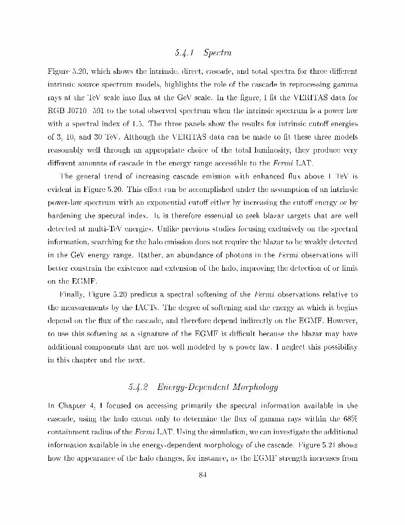
5.4.1 Spe traFigure 5.20, whi h shows the intrinsi , dire t, as ade, and total spe tra for three dierentintrinsi sour e spe trum models, highlights the role of the as ade in repro essing gammarays at the TeV s ale into ux at the GeV s ale. In the gure, I t the VERITAS data forRGB J0710+591 to the total observed spe trum when the intrinsi spe trum is a power lawwith a spe tral index of 1.5. The three panels show the results for intrinsi uto energiesof 3, 10, and 30 TeV. Although the VERITAS data an be made to t these three modelsreasonably well through an appropriate hoi e of the total luminosity, they produ e verydierent amounts of as ade in the energy range a essible to the Fermi LAT.The general trend of in reasing as ade emission with enhan ed ux above 1 TeV isevident in Figure 5.20. This ee t an be a omplished under the assumption of an intrinsi power-law spe trum with an exponential uto either by in reasing the uto energy or byhardening the spe tral index. It is therefore essential to seek blazar targets that are welldete ted at multi-TeV energies. Unlike previous studies fo using ex lusively on the spe tralinformation, sear hing for the halo emission does not require the blazar to be weakly dete tedin the GeV energy range. Rather, an abundan e of photons in the Fermi observations willbetter onstrain the existen e and extension of the halo, improving the dete tion of or limiton the EGMF.Finally, Figure 5.20 predi ts a spe tral softening of the Fermi observations relative tothe measurements by the IACTs. The degree of softening and the energy at whi h it beginsdepend on the ux of the as ade, and therefore depend indire tly on the EGMF. However,to use this softening as a signature of the EGMF is di ult be ause the blazar may haveadditional omponents that are not well modeled by a power law. I negle t this possibilityin this hapter and the next.5.4.2 Energy-Dependent MorphologyIn Chapter 4, I fo used on a essing primarily the spe tral information available in the as ade, using the halo extent only to determine the ux of gamma rays within the 68% ontainment radius of the Fermi LAT. Using the simulation, we an investigate the additionalinformation available in the energy-dependent morphology of the as ade. Figure 5.21 showshow the appearan e of the halo hanges, for instan e, as the EGMF strength in reases from84

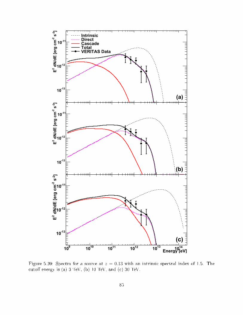
]-2

s-2

dN

/dE

[er

g c

m2

E

-1310

-1210

-1110

(a)

IntrinsicDirectCascadeTotalVERITAS Data

]-2

s-2

dN

/dE

[er

g c

m2

E

-1310

-1210

-1110

(b)

Energy [eV]910 1010 1110 1210 1310 1410

]-2

s-2

dN

/dE

[er

g c

m2

E

-1310

-1210

-1110

(c)Figure 5.20: Spe tra for a sour e at z = 0.13 with an intrinsi spe tral index of 1.5. The uto energy is (a) 3 TeV, (b) 10 TeV, and ( ) 30 TeV.85

DE

C O

ffse

t [d

egre

es]

-2

-1.5

-1

-0.5

0

0.5

1

1.5

2

-1410

-1310

-1210

-1110

-1010

-910

RA Offset [degrees]-2 -1.5 -1 -0.5 0 0.5 1 1.5 2

DE

C O

ffse

t [d

egre

es]

-2

-1.5

-1

-0.5

0

0.5

1

1.5

2

-1410

-1310

-1210

-1110

-1010

-910

Figure 5.21: Extended halo emission for an EGMF strength of B = 10−17 Gauss (top) andB = 10−16 Gauss (bottom).

86

RA Offset [degrees]-2 -1.5 -1 -0.5 0 0.5 1 1.5 2

DE

C O

ffse

t [d

egre

es]

-2

-1.5

-1

-0.5

0

0.5

1

1.5

2

-1510

-1410

-1310

-1210

-1110

-1010

-910

-810

RA Offset [degrees]-2 -1.5 -1 -0.5 0 0.5 1 1.5 2

DE

C O

ffse

t [d

egre

es]

-2

-1.5

-1

-0.5

0

0.5

1

1.5

2

-1510

-1410

-1310

-1210

-1110

-1010

-910

-810

RA Offset [degrees]-2 -1.5 -1 -0.5 0 0.5 1 1.5 2

DE

C O

ffse

t [d

egre

es]

-2

-1.5

-1

-0.5

0

0.5

1

1.5

2

-1510

-1410

-1310

-1210

-1110

-1010

-910

-810

RA Offset [degrees]-2 -1.5 -1 -0.5 0 0.5 1 1.5 2

DE

C O

ffse

t [d

egre

es]

-2

-1.5

-1

-0.5

0

0.5

1

1.5

2

-1510

-1410

-1310

-1210

-1110

-1010

-910

-810

Figure 5.22: Extended halo emission for an EGMF strength of B = 10−16 Gauss at fourdierent energies: 1 GeV (top left), 2.7 GeV (top right), 8.6 GeV (bottom left), and 27 GeV(bottom right). The ir le in the lower left of ea h plot shows the 68% ontainment radiusof the Fermi LAT derived from the a tual spa e raft pointing for RGB J0710+591.10−17 Gauss to 10−16 Gauss for our du ial blazar. The in reasing size of the halo due tothe spreading out of the as ade is readily apparent.In addition to de reasing with the eld strength, the extent of the halo also depends onthe energy of the se ondary gamma rays. Sin e gamma rays of higher energy tend to beprodu ed by ele trons of higher energy, whi h are present earlier in the development of the as ade and are less ae ted by the eld strength, we expe t the extent of the halo to de rease87

Energy [eV]910 1010 1110

Hal

o E

xten

t to

Fer

mi P

SF

Rat

io

-210

-110

1

10

210

Gauss-17B = 10 Gauss-16B = 10 Gauss-15B = 10 Gauss-14B = 10

Figure 5.23: Ratio of the 68% ontainment radius of gamma rays in the halo with respe t tothat of the Fermi LAT for eld strengths from 10−17 to 10−14 Gauss. The intrinsi spe trumof the blazar is a power law with a spe tral index α = 1.5 and a uto energy EC = 10 TeV.as the energy in reases. Figure 5.22 shows that this is indeed the ase. As is apparent inthe gure, both the halo extent and the Fermi PSF de rease with energy. However, above10 GeV, the halo extent de reases mu h more rapidly while the PSF stabilizes to a onstantvalue, as indi ated by Figure 3.2. The signature of the EGMF is therefore an extended halothat be omes pointlike with in reasing energy.The exa t energy at whi h the halo be omes pointlike depends on the eld strength.A good proxy for whether the halo appears pointlike or extended is, of ourse, the ratioof the halo extent to the instrument resolution. If this ratio is near unity, then the halo issu iently extended for the instrument to distinguish it from a point sour e but not so dilutethat it annot be dete ted. Figure 5.23 demonstrates that, under one parti ular assumption88

Cutoff Energy [TeV]1 10

Sp

ectr

al In

dex

1.2

1.4

1.6

1.8

2

2.2

0.1

0.2

0.3

0.4

0.5

0.6

0.7

0.8

0.9

Figure 5.24: Fra tion of gamma rays in the as ade as a fun tion of spe tral index and utoenergy for a blazar at z = 0.13. The white ontour indi ates the region at whi h the total as ade and dire t ux are equal.about the intrinsi spe trum of the blazar, this ratio approa hes unity for some energiesin the Fermi energy range if the eld strength lies between 10−17 and 10−14 Gauss. Wetherefore expe t that a sear h for the energy-dependent morphology of the halo ould delivera positive dete tion of the EGMF if it is within this range.Dis rimination between pointlike and halo emission requires the halo ux to be at least omparable to the dire t ux in the Fermi energy range. Figure 5.24 shows the ratio ofthe ux in the halo to the total ux as a fun tion of the intrinsi spe tral index and utoenergy. The gure mat hes our expe tation that hard sour es with high uto energies willbe as ade-dominated, while sour es with soft spe tra and low uto energies are dominatedby the dire t ux. In the presen e of a magneti eld of su ient strength, larger values of89

this ratio will lead to a stronger halo, whereas when the magneti eld is weak the as adewill enhan e the pointlike emission from the blazar.Blazars are, in general, highly variable obje ts both in the TeV and GeV energy bands.In determining the extent of the halo, we an negle t variability in the TeV range be auseshort-term variations will be averaged out by the as ade pro ess, the time s ale for whi h an be on the order of 106 years. It is therefore important only to a hieve an unbiased pi tureof the TeV emission over long time periods, averaging aring states with periods of quies entemission. However, the halo in the GeV range will of ne essity be onstant, sin e it is theaverage emission over the long time s ales in the as ade. While variability in the Fermiobservations is not ruled out by our model, we do expe t any variability to be pointlike.5.4.3 Time ProlesIn addition to the information available from the halo, it is possible to onstrain the EGMFbased on the time delays of gamma rays in the as ade with respe t to the arrival of a areof dire t gamma rays. Sin e blazars are highly variable sour es in the TeV energy band,we expe t a hara teristi de ay of the light urve that is dependent on the eld strength.Although su h an investigation is beyond the s ope of this work, it is in prin iple possibleto dete t this de ay if the eld strength is su iently weak, as indi ated by Figure 5.25, inwhi h the time delays of gamma rays in the as ade are plotted for eld strengths of 0 and10−18 Gauss. The average time delays for these three ases are, respe tively, 10 minutes and2 weeks. In the absen e of eviden e for a halo, the EGMF ould be as weak as 10−18 Gaussif the blazar lifetimes are shorter than the time s ales on whi h the as ade rea hes steadystate, in whi h ase observations of the existen e or absen e of a de ay in the light urvefollowing a are ould be used to measure or onstrain the eld.

90

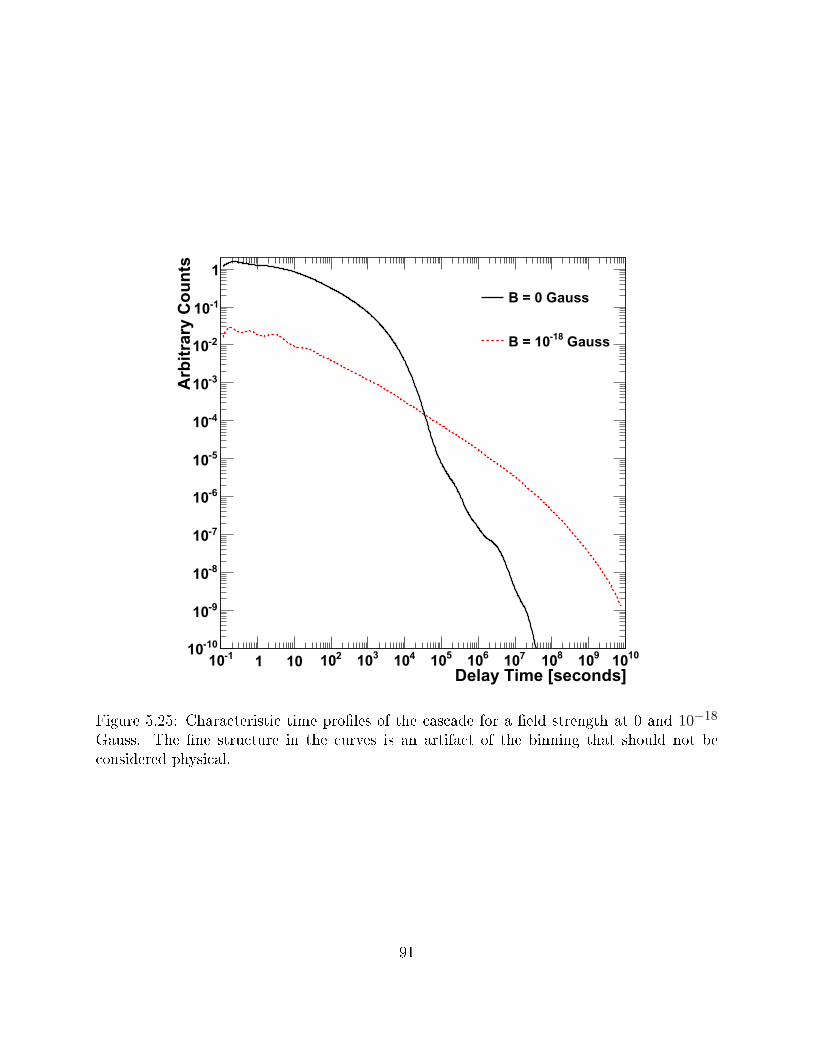
Delay Time [seconds]-110 1 10 210 310 410 510 610 710 810 910 1010

Arb

itra

ry C

ou

nts

-1010

-910

-810

-710

-610

-510

-410

-310

-210

-110

1

B = 0 Gauss

Gauss-18B = 10

Figure 5.25: Chara teristi time proles of the as ade for a eld strength at 0 and 10−18Gauss. The ne stru ture in the urves is an artifa t of the binning that should not be onsidered physi al.91

CHAPTER 6THE SEARCH FOR BLAZAR HALOS IN THE EGMFCONTEXTIn this hapter, I present the results from a sear h for halos around sele t blazars and theinterpretation of those results in the ontext of the EGMF. The Monte Carlo simulationdes ribed in Chapter 5 permits us to hara terize the energy-dependent morphology of the as ade in the energy range a essible to the Fermi instrument, as well as to predi t thespe trum measured by ground-based IACTs. While observations in these two energy bandsindividually are not very onstraining, their ombination an very strongly onstrain theproperties of the EGMF.Using the semi-analyti model presented in Chapter 4, we found a lower limit on theEGMF strength of ∼ 3 × 10−16 Gauss, but it was di ult to a ess the energy-dependentmorphology of the halo of gamma rays around the blazar. The Monte Carlo simulation allowsus to predi t this halo straightforwardly and ompare it to existing blazar observations. Iuse the simulation to ondu t a general sear h for the spe i energy-dependent morphologyof the halo. 6.1 AssumptionsThe interpretation of blazar halos is dependent on a large parameter spa e in luding thespe tral properties of the sour e, the EBL, and the model for the EGMF. The di ulty ofexploring this parameter spa e ne essitates some assumptions regarding its properties. Asin the rest of this work, I adopt the relatively low EBL model of Fran es hini et al. (2008).For the EGMF model, I use a simple model that divides the volume of spa e into ubi domains of length L within whi h the eld strength is onstant. The orientation of theeld within a domain is xed to a random value independent of any other domain, so thatL is representative of the orrelation length as spe ied by Equation 1.2. The eld strengthis xed to a onstant value that is the same for every domain. In this way, we sear h for thedominant omponent of the EGMF in the voids of the LSS.For blazars with a well measured redshift, the bulk of the remaining parameter spa e omprises hara teristi s of the spe trum intrinsi to the blazar itself. In ases where infor-92

mation on the properties of the blazar is available, we an use that information to narrowthe parameter spa e. However, in general the time prole, relativisti beaming, and exa tshape of the intrinsi spe trum are unknown. In su h ases we estimate values that seem rea-sonable for an average blazar. The dominant parameters ae ting the as ade are of oursethe spe tral index and uto energy from Equation 3.1, sin e these two parameters ontrolthe level of the intrinsi ux in the TeV energy range that auses the as ade. As shown inFigure 5.24, these parameters strongly govern the apability of our sear h to dete t a halo.We therefore allow these parameters to vary in our sear h while xing all other parametersto reasonable estimates. 6.1.1 The Time ProleAs emphasized in Chapter 4, reliable blazar observations simultaneous in both the GeV andTeV energy ranges are limited to the past ∼ 3 years. However, the time for gamma raysin the as ade to a hieve a steady state an be on the order of 106 years, and there is noguarantee that the urrent a tivity of the blazar is representative of the a tivity over itslifetime. Periods of higher or lower a tivity in the past ould ae t the presently observedux. Sin e 106 years is relatively short for gala ti time s ales, we therefore generally assumethat the urrent observations of the blazar are representative of its average a tivity.An additional ompli ation is introdu ed be ause blazars are highly variable obje ts thattend to emit strong ares. As long as the EGMF is relatively strong, ares in the as adewill be averaged over the as ade time s ale and we expe t no time variation of the uxin the as ade. However, observations in the TeV band are sparse be ause the IACTs arepointed instruments, and the rate of aring is unknown. Our adoption of a steady timeprole for the ux therefore additionally assumes that the existing IACT observations arerepresentative of the a tual aring rate averaged over the blazar lifetime.6.1.2 Relativisti BeamingChapter 3 motivated the model of a blazar as relativisti populations of ele trons boostedto a bulk Lorentz fa tor Γ, resulting in highly beamed obje ts. In the absen e of dire tmeasurements, we assume that Γ = 10, in a ord, for example, with average measured valuesfrom misaligned AGN as determined by Hovatta et al. (2009). We furthermore assume that93

the viewing angle between the blazar jet dire tion and the line of sight to Earth is θV = 0.We expe t that the viewing angles of gamma-ray-dete ted AGN will be small be ause theopening angle of the beamed emission, whi h an be approximated as Γ−1 ≈ 5, is relativelysmall. While misaligned AGN may exhibit halos, the dire t ux in the TeV band is mu hweaker than in the aligned ase (Neronov et al., 2010), making reliable estimates of theintrinsi spe trum that produ es the as ade di ult.6.1.3 Simulation LimitsAs the ele trons enter the Thomson regime, the number of gamma rays they produ e in- reases inversely with the minimum energy for the gamma rays to be deemed observable,requiring roughly an order of magnitude more simulation time for every de ade in energy.We therefore restri t our attention to as ade gamma rays above 1 GeV, ignoring any uxmeasured by Fermi from 100 MeV to 1 GeV. Sin e the lower-energy gamma rays are moresensitive to lower eld strengths, the overall ee t of this limitation is to raise the lower limiton the range of EGMF strengths to whi h our method is sensitive. However, given the at-tening near 1 GeV of the urves in Figure 5.23, it is unlikely that in luding this informationwould substantially improve the sensitivity of our method.6.1.4 The Intrinsi Spe trumWe assume that Equation 3.1 adequately models the blazar's intrinsi spe trum over theenergy range from 1 GeV to 10 TeV. By s anning the spe tral index α from 1.1 to 2.1 andthe uto energy EC from 200 GeV to 50 TeV, we explore the parameter spa e in a sear hfor the as ade model that best ree ts the existing observations for a parti ular blazar. Ourassumed limits on α and EC are parti ularly reasonable when the best-t value is not at theedges of the spa e. In addition to avoiding an innite-energy atastrophe, the exponential uto is physi ally motivated be ause primary gamma rays above 50 TeV are likely to intera tsu iently lose to the blazar so that the ele trons they produ e sample not the EGMF inthe voids, but rather the magneti eld lo al to the luster hosting the blazar, as suggestedby Figure 2.11. The very strong luster eld then isotropizes the ele trons so that theirups attered emission forms an insigni ant ontribution to the as ade. The exponential uto an a ount for this lost ux in a natural way.94

In prin iple, we ould use additional information from low-energy observations to on-strain the blazar spe trum further. However, we deliberately avoid this so that our on- lusions are not based on any spe i model of blazar emission. The models an be quite ompli ated, involving many parameters, and the existen e of orphan ares (Kusunose &Takahara, 2006) implies that the emission me hanisms in blazars are not fully understood.An introdu tion to the basi s of blazar modeling an be found in Aharonian (2004).6.1.5 The EGMF ModelWe assume that the orrelation length of the magneti eld is L0 = 1 Mp , roughly the lengthover whi h an energeti ele tron ools to ∼ 50 GeV, so that over their lifetimes the ele tronssample only a single EGMF domain. If the orrelation length is smaller, the ele trons beginto experien e a random walk a ross many domains, redu ing the inuen e of the EGMFon the ele trons' dee tions. If halo features are predi ted at a given angular size θ for a orrelation length of L0, then their apparent size when L≪ L0 is, very roughly (Neronov &Semikoz, 2009),θ′ ≈

√

L

L0θ. (6.1)A lower limit on the EGMF strength of B when L = L0 will therefore be ome even more onstraining if the orrelation length is signi antly smaller, sin e the eld must be strongerthan B to a hieve the same dee tion of the ele trons.6.1.6 Properties of the Cas adeCertain assumptions regarding the properties of the as ade are also ne essary for the inter-pretation of halo data. Essey & Kusenko (2010) have noted that, sin e AGN may be sour esof osmi -ray nu lei, there ould be an additional omponent to the as ade that arises dueto osmi -ray intera tions with the EBL. Some observational eviden e su h as the existen eof blazars at z > 0.1 with spe tra that must be ex eptionally hard to over ome the EBLattenuation may support this idea (Essey & Kusenko, 2011). However, it remains an openquestion whether signi ant osmi -ray produ tion o urs in blazars, so we assume that the osmi -ray produ tion by the blazars studied in this work is negligible.We also make the assumption that inverse Compton and pair produ tion are the dominant95

me hanisms for energy loss in the as ade. Re ently, Broderi k et al. (2011) pointed out thatthe as ades may be sus eptible to plasma instabilities due to the ele trons' intera tions withthe ba kground of ionized hydrogen in extragala ti spa e, arguing that the rate of energyloss due to plasma instabilities is mu h larger than that due to inverse Compton s attering.A detailed study of the instabilities remains to be undertaken, however, and the pre isenature of the role of plasma instabilities in the as ade is presently un lear. La king furtherinformation, we assume that this ee t an be negle ted.6.2 Data AnalysisData from both ground-based IACTs and the Fermi LAT are ne essary for onstraining theEGMF. On e the data are in hand, we pro eed in the analysis by assuming a ombinationof intrinsi spe tral index α, uto energy EC , and EGMF strength B. For a given pointin the parameter spa e, we use the results of the Monte Carlo simulation to predi t theenergy spe trum in the TeV range, along with the detailed energy-dependent morphologyof the as ade in the GeV energy range. We explore the spa e by hoosing 12 values of αfrom 1.1 to 2.1, 12 values of EC from 200 GeV to 50 TeV, and 13 values of B, 12 evenlylogarithmi ally spa ed from 10−18 Gauss to 3.2× 10−13 Gauss, as well as 0 Gauss, resultingin a parameter spa e of 1,872 separate models. We then t the data to those predi tions. Atthe point of tting, the total luminosity of the sour e is the only remaining free parameter,and we determine the best-t value onsistent with data from both energy ranges.6.2.1 Ground-Based InstrumentsAs dis ussed in Se tion 3.3, the present generation of IACTs in ludes VERITAS, HESS, andMAGIC, all of whi h have dete ted a number of blazars in the TeV energy range1. Thesensitivities of these instruments extend from ∼ 100 GeV to greater than 30 TeV. We usethe IACT observations to determine reliable spe tra in the TeV-energy range in order tointerpret the observed properties of a hypotheti al halo resulting from intera tions betweenthe primary gamma rays and the EBL and CMB. Toward that end, we use the publishedspe tra on spe i blazars from observations performed by these instruments. Be ause these1. A detailed atalog of TeV sour es an be found at http://tev at.u hi ago.edu/.96

spe tra are typi ally derived under the assumption that the sour e is pointlike, we musta ount for possible halo extension in the TeV energy range. We a omplish this with asimple, energy-independent model of the total gamma-ray PSF of the instrument, derivedfrom Aharonian et al. (2006). The exa t shape of the PSF is relatively unimportant, and weignore any possible dependen e on the energy of the measured gamma rays.We next pro eed by applying the simple PSF model to the simulated predi tions in theTeV energy range. Re alling from Se tion 3.3 that a ut on θ2 is used to dene the point-sour e region in an IACT analysis, we ount only the simulated photons that fall withinthe θ2 ut, obtaining a predi tion F0 for the ux. Sin e the model of the PSF is known,we know the probability p for a pointlike gamma ray to be re onstru ted within the θ2 ut, and so we an orre t the ux to obtain the true ux F = F0/p. Obviously, thispro edure does not determine the orre t value of the ux if there is a halo present be ausethe probability for a halo gamma ray to be re onstru ted within the θ2 ut is less than pdue to its extension. Rather, this pro edure mimi s the analysis ondu ted to obtain thepublished spe trum, produ ing a value that an be ompared to the published results andadditionally a ounting for any possible extension due to the halo, whi h an be important,espe ially at lower energies. 6.2.2 Fermi DataWe analyze publi ly available data from more than three and a half years of Fermi LATobservations starting in August 2008 and ending in Mar h 2012 to determine the ux inthe GeV range. Our analysis employs version v9r23p1 of the Fermi tools, with the on-orbitinstrument response fun tions P7SOURCE_V62. In ontrast to the analysis dis ussed inChapter 4, in whi h we al ulated the spe trum within the 68% ontainment radius of theFermi PSF, we fully hara terize the energy-dependent morphology of the as ade in aneort to maximize our use of the available information. After a binned analysis onsisting ofevent sele tion, the reation of ounts maps, and exposure omputation, we ondu t 1,872separate likelihood analyses to assess the probability of every model in our parameter spa e.For the pre-likelihood analysis, we sele t events of lass 2, whi h are intended for general2. Further information on Fermi data analysis is available at the Fermi S ien e Support Center's website,http://fermi.gsf .nasa.gov/ss /. 97

sour e analysis. We also adopt a region of interest (ROI) size appropriate for analysisabove 1 GeV of 20, a ounts ube size of 28, and an exposure ube size of 70. Duringthe likelihood analysis, we in lude all sour es within 30 of the position of our analyzedblazar, xing all parameters of those sour es greater than 10 from the ROI enter andkeeping free only the normalization for sour es between 2 and 10 from the enter. Wealso in lude the extragala ti diuse model iso_p7v6sour e and the Gala ti diuse modelgal_2yearp7v6_v0.In order to in lude the predi ted energy-dependent morphology of the blazar in our analy-sis, we es hew the standard Fermi point-sour e models and employ instead a MapCubeFun -tion, whi h is the same type of model used for the Gala ti diuse ux. The MapCubeFun -tion permits us to spe ify any arbitrary halo morphology at dis rete energies. In onstru tingthese sour e models from the simulated data, we use an ideal PSF that leaves the simulatedgamma rays' dire tions unaltered, and we allow the gtsr maps tool to a ount for the FermiIRFs.Be ause the Gala ti diuse model is highly detailed, it o upies a large amount of omputer memory. In order to redu e the memory requirements for a single run and thusfa ilitate the parallel pro essing of the 1,872 jobs, we repla e the Gala ti diuse map with asmaller version trimmed to a 60 by 60 region entered on the position of the blazar. Thissmaller region will ontain with very high ertainty all of the gamma rays from the Gala ti diuse that ould be re onstru ted into our ROI. We verify that our trimmed version of theGala ti diuse produ es the same results as the full version by running standard likelihoodanalyses using both models. The Point Sour e row in Table 6.1 shows that these analysesare not substantially dierent. Additionally, we investigated whether dierent eld models ould be ae ted by the ut Gala ti diuse model, sin e the extent of the sour e dependson the eld and this ould make our results sensitive to other extended sour es su h as theGala ti diuse. Sele ting a uto energy of 11 TeV and a spe tral index of 1.55 and tryingthree separate elds, we nd that the ut Gala ti diuse model has little impa t on thetest statisti of the sour e for the elds, as shown in the lower three rows of Table 6.1. Weare therefore ondent that the ut Gala ti diuse model does not strongly inuen e ourresults and we use it routinely in our analysis.98

Full Diuse Model Cut Diuse ModelSour eTS Sour eFlux DiuseFlux Sour eTS Sour eFlux DiuseFluxPointSour e 166.98 6.72±1.24

0.987±0.013

166.87 6.69±1.12

1.025±0.014

B = 0Gauss 159.98 0.562±0.084

0.987±0.012

159.88 0.561±0.084

1.025±0.013

B = 10−16Gauss 156.24 0.657±0.099

0.987±0.012

156.09 0.655±0.099

1.025±0.013

B = 10−13Gauss 164.40 2.61±0.40

0.987±0.012

164.32 2.60±0.40

1.025±0.013Table 6.1: Results from Fermi data analyses with the full Gala ti diuse and ut Gala ti diuse models for the blazar RGB J0710+591. The Gala ti diuse uxes are with respe tto the nominal value. The sour e uxes are in 10−10 gamma rays m−2 s−1 for the pointsour e and relative to the best-t TeV spe trum for the spe i eld models. Although the ut Gala ti diuse ux is systemati ally high by a slight amount, the test statisti for thesour e is not substantially dierent between the full and ut models.6.2.3 Combining the DataFor the TeV data, we t our predi ted urve to a set of data points representing the mea-sured spe trum, obtaining the χ2 value of the t. If we assume that the data are normally

99

distributed, then we an write χ2 asχ2 = −2 ln(LTeV), (6.2)where LTeV is the likelihood. The Fermi data analysis yields a test-statisti value T givenbyT = −2 ln

(

L0

LGeV) , (6.3)where L0 is the maximum likelihood of the data under the null hypothesis that no sour eis present, and LGeV is the maximum likelihood for the sour e model given the data. Byinspe tion of Equations 6.2 and 6.3, it is lear we an multiply the likelihoods LTeV andLGeV by onstru ting a total test statisti χ2−T . Compared to the χ2 value, the Fermi teststatisti T is likely to be very large for strong sour es be ause it is al ulated with respe t tothe null hypothesis. However, when omparing two models, we are interested in the dieren ebetween the al ulated values of χ2 −T , and the overall s ale is unimportant (James, 2006).For ea h of the 1,872 models, we onstru t the total test statisti values χ2 − T , leavingthe total luminosity as the only free parameter des ribing the blazar. This is a omplished byperforming repeated Fermi likelihood analyses with the luminosity xed, adding the χ2 valuefor the given luminosity, and adaptively s anning the luminosity spa e until the variationbetween points is su iently small. A paraboli t to the measured points determines thenal best-t value for the ombined statisti . We then proje t the total statisti onto theEGMF strength in a manner similar to our analysis in Se tion 4.2. By nding the point atwhi h this urve surpasses its minimum by a ertain value, we an measure or onstrain theeld at a desired level of onden e.6.3 Data Veri ationDete ting the relatively weak halo on top of the pointlike emission from the blazar requiresa solid understanding of the Fermi instrument response. In order to gain onden e thatthe sear h des ribed in this hapter would allow us to dete t a halo if it did exist, wehave ondu ted a set of rigorous tests to ensure the a ura y and stability of the method.Throughout this se tion, we fo us on results from the blazar RGB J0710+591 to illustrateour data veri ation pro edure. 100

6.3.1 Pro edureThe testing pro edure begins by sele ting one of the 1,872 models and assuming that itgives the orre t distribution of gamma rays from the sour e, whi h we refer to as the testmodel. Due to their large errors, in general the TeV data an be made to t the spe trumwell simply via the sele tion of an appropriate luminosity and su iently large uto energy,as shown in Se tion 5.4.1. Given that the VERITAS data on RGB J0710+591 extend to ∼ 6TeV, however, it is unlikely that the TeV data will plausibly be drawn from the test modeldistribution unless the uto energy is hosen to be above ∼ 1 TeV. Nevertheless, we ndthat it an be instru tive to in lude su h models in the veri ation, so we pla e no limit onthe intrinsi spe trum, and we fo us on assessing the validity of the GeV-s ale predi tions.We use the Fermi tool gtobssim to generate a simulated data set for the Fermi LATusing the a tual pointing history of the spa e raft and a spe ied set of gamma-ray sour es.Our simulated data set overs a time range of 108 se onds, slightly more than three years,beginning on 15 August 2008. For the sour es we use the same set that we sele ted inSe tion 6.2.2, pla ing our test model for the blazar at the enter of the ROI. Sin e some ofthe sour es' spe tra are modeled by fun tions that are unavailable to the gtobssim tool, we onvert these spe tra to power laws with similar normalization, expe ting that the resultsof ts to the simulated data with these repla ements will en ompass only minor hanges.We then treat the simulated data as real data, passing them through the analysis hainand nding the best-t ombined statisti for all 1,872 models, without using our knowledgeof the true intrinsi spe trum to aid our analysis in any way. After proje ting onto theeld-strength axis, we expe t with high onden e that the known orre t eld strengthfrom the test model will be within the allowed region.Running the veri ation pro edure is highly pro essor-intensive. From start to nish,a single simulated data set requires more than 104 ore-hours of pro essing time. For thisreason, it is omputationally infeasible to run many simulations for one test model anddemonstrate that the onden e level a urately ree ts the probability of nding the or-re t eld strength from the test model within the quoted range. It is also time- onsumingto pro ess additional models; in total we use four separate models in the data veri ationpro edure, one whi h we sele t with mali e aforethought to give results similar to the realobservations in the Fermi energy band, and three whi h we hoose at random using a om-101

Test Field [Gauss α EC Counts Fit Field [Gauss TeV χ2/dof1 3 × 10−16 1.55 18 TeV 132 (3.9 ± 1.6) × 10−16 1.77/42 10−18 1.9 200 GeV 1878 none 21.7/43 3 × 10−16 1.83 50 TeV 214 none 2.11/44 10−15 1.19 30 TeV 70 (4.8 ± 3.4) × 10−16 1.98/4Table 6.2: Parameters from one predetermined and three randomly sele ted models for theintrinsi spe trum of RGB J0710+591.puter program. These latter three ases an therefore be thought of as double-blind testsof the analysis pro edure. A summary of these tests, along with the parameters for theirintrinsi spe tra, the true eld, the eld re onstru ted at 68% onden e, and the observednumber of ounts asso iated with our sour e, appears in Table 6.3.1. For two of these mod-els, Tests 2 and 3, the blazar parameters are lo ated in a region of Figure 5.24 unfavorableto halo dete tion. Consequently, our pro edure fails to re onstru t any eld strength. Tests1 and 4, however, are in a favorable region for halo dete tion. In Test 1, the true eld iswell within the error range at 68% onden e, and for Test 4 the true eld is only slightlyoutside this range. Sin e our overall method is sensitive only to the order of magnitude ofthe eld strength, we expe t that this veri ation pro edure is adequate.6.3.2 TestsFor our rst test, we sele t a test model with a spe tral index of α = 1.55, a uto energyEC = 18 TeV, and a eld strength of B = 3 × 10−16 Gauss. This model is al ulated toprovide a high level of statisti s for dete ting the halo in an EGMF range for whi h the halosize is omparable to the instrument PSF. As a rst test, it demonstrates the apability ofthe sear h to dete t a halo in the optimum situation of a hard, high-energy sour e and amagneti eld amenable to produ ing a halo in the Fermi energy range. We summarize theresults of this rst test in Figure 6.1, in whi h it is evident that the orre t eld is well withinthe re onstru ted range of B = (3.9± 1.6)× 10−16 Gauss. This gives us onden e that ouranalysis pro edure an re onstru t the eld in an optimisti ase.As is evident by the number of ounts shown in Table 6.3.1, the three double-blind102

Field Strength [Gauss]-1910 -1810 -1710 -1610 -1510 -1410 -1310

Cu

toff

En

erg

y [T

eV]

1

10

Field Strength [Gauss]-1910 -1810 -1710 -1610 -1510 -1410 -1310

Sp

ectr

al In

dex

1

1.2

1.4

1.6

1.8

2

2.2

Field Strength [Gauss]-1910 -1810 -1710 -1610 -1510 -1410 -1310

Lik

elih

oo

d S

tati

stic

-138

-136

-134

-132

-130

-128

-126

Test 1 Results

95% Measurement Gauss-17 10×B > 9 Gauss-15 10×B < 3

99% Limit

Gauss-17 10×B > 4

Figure 6.1: Summary of the results of Test 1 from Table 6.3.1. The best-t spe tral index and uto energy as a fun tion of eld strength appear in the top left and top right, respe tively.The bottom left panel shows the likelihood statisti urve as a fun tion of EGMF strength,while the bottom right panel summarizes the on lusions that an be drawn about the eldstrength for this test. The points at 10−19 Gauss are a tually omputed at 0 Gauss. Thered bars indi ate the 1-σ and 95% onden e measurements of the eld.tests fortuitously overed a wide range of intrinsi sour e models leading to very dierentpredi tions in the Fermi energy band. In the rst test, the intrinsi spe trum spe trum isvery pessimisti for dete ting a halo: the spe tral index is very soft at 1.9 and the utoenergy of 200 GeV is as low as our analysis pro edure tests. For this reason, even the TeV103

Cutoff Energy [TeV]1 10

Sp

ectr

al In

dex

1.2

1.4

1.6

1.8

2

-4500

-4000

-3500

-3000

-2500

-2000

-1500

Cutoff Energy [TeV]1 10

Sp

ectr

al In

dex

1.2

1.4

1.6

1.8

2

-4500

-4000

-3500

-3000

-2500

-2000

-1500

Cutoff Energy [TeV]1 10

Sp

ectr

al In

dex

1.2

1.4

1.6

1.8

2

-4500

-4000

-3500

-3000

-2500

-2000

-1500

Cutoff Energy [TeV]1 10

Sp

ectr

al In

dex

1.2

1.4

1.6

1.8

2

-4500

-4000

-3500

-3000

-2500

-2000

-1500

Figure 6.2: Likelihood statisti maps for Test 2 from Table 6.3.1. The EGMF strength inGauss is 10−17 (top left), 10−16 (top right), 10−15 (bottom left), and 10−14 (bottom right).t to the spe trum alone is rather poor: the χ2 of the t per degree of freedom is 21.7/4, orresponding to a probability of 2.3×10−4. The total luminosity must be greatly in reasedin order to a hieve even this poor t, and the very soft spe trum onsequently di tatesthat the Fermi emission must be very high, leading to the produ tion of a large numberof gamma-ray ounts. Additionally, the eld strength of 10−18 Gauss is very low, implyingthat the halo will be undete table and all of this very strong Fermi emission will appearpointlike, further softening the spe trum.It is instru tive to look at the likelihood statisti maps as a fun tion of uto energyand spe tral index, whi h appear in Figure 6.2 for four dierent values of the eld strength.104

In general, when the spe tral index is soft, the models tend to t well independent of the uto energy, sin e there are very few gamma rays with su ient energies to generate thehalo. For all elds, hard spe tra with low uto energies t poorly be ause there is againno halo, and the hard spe tral index is a poor mat h to the true spe tral index of 1.9 inthe GeV energy range. For low elds, this problem an be remedied by moving to higher uto energies, where there is still no halo sin e the eld is weak, but the overall ee t of the as ade is to soften the spe trum, as anti ipated by Figure 5.20, toward the orre t value.When the eld is strong, however, the as ade spreads out into the halo, and this softeningis no longer possible, explaining the very poor ts in the bottom right orner of the plot forthe 10−15 and 10−14 Gauss ases.Figure 6.3 summarizes the results of the se ond test. It is obvious that the orre t valuesof soft spe tral index and low uto energy are strongly favored. As expe ted, this modelprovides no sensitivity to the EGMF strength. In fa t, the trend in the bottom left plot ofFigure 6.3 appears to be slightly negative, in the wrong dire tion. However, this trend ishardly signi ant, given the s ale of the plot.In the third test, the spe tral index is again soft at 1.83 but the uto energy is anextremely high 50 TeV. As shown in Table 6.3.1, the t to the TeV data is very good, sounlike the previous test we expe t this test to ree t a plausible situation for the blazar, giventhe TeV data alone. The eld strength for this test is right in the range where we shouldbe able to dete t it, so the only question is whether the high uto energy an win out overthe soft spe tral index and produ e a large enough halo signal to be dete ted. However,Figure 5.24 shows that the expe ted fra tion of gamma rays in the halo for this ase is verynearly omparable to the fra tion of dire t gamma rays, so we do not expe t the results tobe very onstraining. Additionally, a ording to Table 6.3.1, there are fewer gamma raysin this test. This is mainly due to the higher uto energy that permits a more reasonabletotal luminosity to be t to the TeV data. We therefore expe t that this test will have littlesensitivity to the eld strength, and that the overall s ale of the likelihood urve will besmaller in magnitude that in the se ond test, owing to the smaller number of gamma raysasso iated with the sour e. Figure 6.4 onrms these expe tations.The fourth test also ts the TeV data very well. Although the uto energy is high at30 TeV, the intrinsi spe trum for this test is rather weak when the hard spe tral indexα = 1.19 is extrapolated to lower energies, so the number of simulated Fermi gamma rays is105

Field Strength [Gauss]-1910 -1810 -1710 -1610 -1510 -1410 -1310

Cu

toff

En

erg

y [T

eV]

1

10

Field Strength [Gauss]-1910 -1810 -1710 -1610 -1510 -1410 -1310

Sp

ectr

al In

dex

1

1.2

1.4

1.6

1.8

2

2.2

Field Strength [Gauss]-1910 -1810 -1710 -1610 -1510 -1410 -1310

Lik

elih

oo

d S

tati

stic

-4483

-4482.8

-4482.6

-4482.4

-4482.2

-4482

-4481.8

-4481.6

-4481.4

-4481.2

-4481

Test 2 Results

95% Limit

none

99% Limit

none

Figure 6.3: Summary of the results of Test 2 from Table 6.3.1. The best-t spe tral index and uto energy as a fun tion of eld strength appear in the top left and top right, respe tively.The bottom left panel shows the likelihood statisti urve as a fun tion of EGMF strength,while the bottom right panel summarizes the on lusions that an be drawn about the eldstrength for this test. The points at 10−19 Gauss are a tually omputed at 0 Gauss.relatively low. The eld of 10−15 Gauss is well within the dete table range, and a ordingto Figure 5.24, the Fermi energy range should be dominated by halo gamma rays. As shownin Figure 6.5, our pro edure re onstru ts the eld to be B = (4.8± 3.4)× 10−16 at the 68% onden e level. The true eld lies just slightly outside this range, but this is not surprisingsin e the probability for this o uring is about 32%. At 95% onden e, our method allows106

Field Strength [Gauss]-1910 -1810 -1710 -1610 -1510 -1410 -1310

Cu

toff

En

erg

y [T

eV]

1

10

Field Strength [Gauss]-1910 -1810 -1710 -1610 -1510 -1410 -1310

Sp

ectr

al In

dex

1

1.2

1.4

1.6

1.8

2

2.2

Field Strength [Gauss]-1910 -1810 -1710 -1610 -1510 -1410 -1310

Lik

elih

oo

d S

tati

stic

-183

-182.8

-182.6

-182.4

-182.2

-182

-181.8

-181.6

-181.4

-181.2

-181

Test 3 Results

95% Limit

none

99% Limit

none

Figure 6.4: Summary of the results of Test 3 from Table 6.3.1. The des ription of the plotsis the same as in Figure 6.1.only a lower limit to be pla ed on the eld strength, and in this ase we nd B > 4× 10−17Gauss, and the true eld is learly allowed.The results of the data veri ation tests indi ate that our pro edure an a urately re- onstru t the eld strength in the event that a halo is dete table. Furthermore, the behaviorof the ts mat hes our expe tations from a qualitative analysis of ea h tested situation. Asindi ated in Figure 5.23, dete table eld strengths range from ∼ 10−17 to ∼ 10−14 Gauss,above whi h the halo be omes too extended in the Fermi data for it to be distinguished107

Field Strength [Gauss]-1910 -1810 -1710 -1610 -1510 -1410 -1310

Cu

toff

En

erg

y [T

eV]

1

10

Field Strength [Gauss]-1910 -1810 -1710 -1610 -1510 -1410 -1310

Sp

ectr

al In

dex

1

1.2

1.4

1.6

1.8

2

2.2

Field Strength [Gauss]-1910 -1810 -1710 -1610 -1510 -1410 -1310

Lik

elih

oo

d S

tati

stic

-44

-43

-42

-41

-40

-39

-38

-37

-36

Test 4 Results

95% Limit

Gauss-17 10×B > 4

99% Limit

none

Figure 6.5: Summary of the results of Test 4 from Table 6.3.1. The des ription of the plotsis the same as in Figure 6.1.from the Gala ti and extragala ti diuse ba kgrounds. This upper limit should of oursebe onsidered rather loose; although it is true that the Fermi PSF may be similar to thehalo size at large energies when the eld is as strong as 10−14 Gauss, the ux of gammarays generally de reases with energy, and Fermi may not olle t enough gamma rays to beable to distinguish between the extended halo and a point sour e. With a high degree of onden e, however, we an sear h for EGMF strengths near ∼ 10−16 Gauss using our haloanalysis pro edure. 108

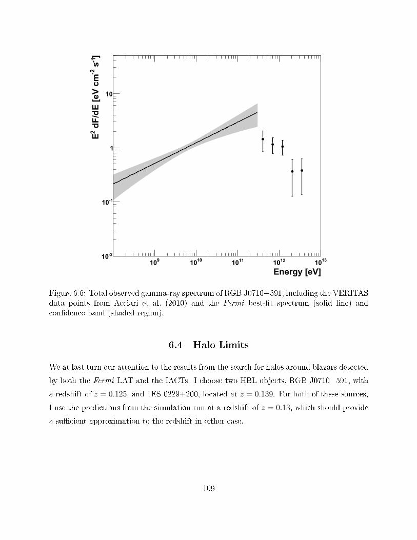
Energy [eV]

910 1010 1110 1210 1310

]-1

s-2

dF

/dE

[eV

cm

2E

-210

-110

1

10

Figure 6.6: Total observed gamma-ray spe trum of RGB J0710+591, in luding the VERITASdata points from A iari et al. (2010) and the Fermi best-t spe trum (solid line) and onden e band (shaded region). 6.4 Halo LimitsWe at last turn our attention to the results from the sear h for halos around blazars dete tedby both the Fermi LAT and the IACTs. I hoose two HBL obje ts, RGB J0710+591, witha redshift of z = 0.125, and 1ES 0229+200, lo ated at z = 0.139. For both of these sour es,I use the predi tions from the simulation run at a redshift of z = 0.13, whi h should providea su ient approximation to the redshift in either ase.109

6.4.1 RGB J0710+591In Chapter 4, we pla ed limits on the strength of the EGMF based on spe tral data from theblazar RGB J0710+591, whi h is lo ated at a right as ension of 07h10m26.4s (107.625) andde lination of +5909′00′′ (59.139). The total spe trum of this blazar appears in Figure 6.6,in whi h the TeV-s ale data points from the VERITAS observations (A iari et al., 2010)and the GeV-s ale data points from our own analysis are shown. We derive the Fermi datapoints using an unbinned likelihood analysis under the assumption that the spe trum is wellmodeled by a power law a ross the entire energy range a essible to Fermi. Additionally, wein lude the likelihood onden e band from the overall power-law t to the total data setfrom 100 MeV to 300 GeV.We ondu t a binned Fermi analysis of the data in the vi inity of RGB J0710+591 asdes ribed in Se tion 6.2.2, after whi h we apply our analysis pro edure to sear h for theextended halo emission. Figure 6.7 shows the likelihood statisti maps for the analysis,using the same elds that were presented in Se tion 6.3.2. It is lear that the results favoran EGMF that is relatively strong, sin e the minimum of the maps ontinues to de rease asthe eld strength in reases.Figure 6.8 summarizes the information from the analysis performed on RGB J0710+591.The best-t uto energies and spe tral indi es lie well within the sear h range, giving us onden e that we have su iently explored the parameter spa e. The in rease of both the uto energy and spe tral index with eld strength is driven by the need to mat h the IACTobservations. That is, if the uto energy is low, within the TeV data, then the spe tral indexshould be ome harder in order to mat h both ends of the TeV spe trum. Correspondingly,as the uto energy in reases, it no longer ae ts the TeV data points, whi h are then bestt by a slightly softer power law.Although our likelihood urve is insu ient for limiting the eld at 99% onden e, wedo a hieve a 95% onden e limit of B > 7 × 10−16 Gauss. We interpret this limit as theabsen e of a halo. Our result validates previous results that used the spe tral data aloneto suggest that the strength of the EGMF is greater than ∼ 10−16 Gauss (Taylor et al.,2011). As anti ipated by Figure 5.23, the likelihood urve attens out above 10−14 Gauss,where our method be omes insensitive to the large extended halo around the point sour e.By sele ting other blazar targets and applying the same analysis, we therefore expe t that110

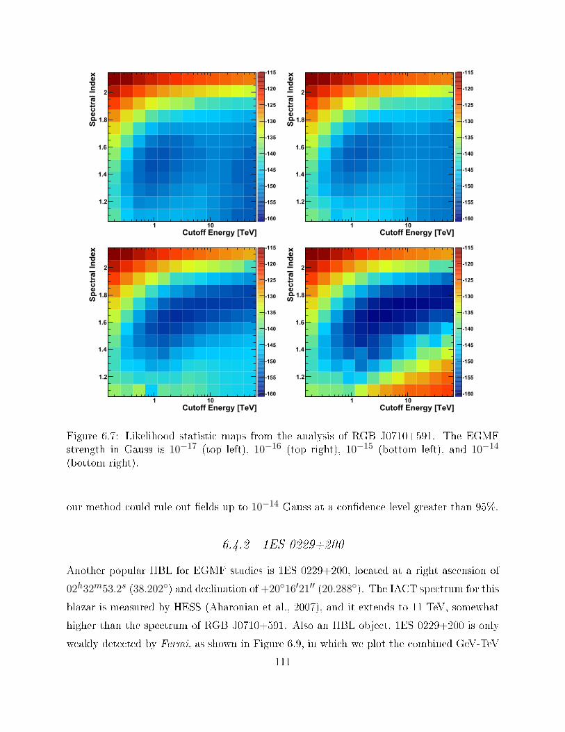
Cutoff Energy [TeV]1 10

Sp

ectr

al In

dex

1.2

1.4

1.6

1.8

2

-160

-155

-150

-145

-140

-135

-130

-125

-120

-115

Cutoff Energy [TeV]1 10

Sp

ectr

al In

dex

1.2

1.4

1.6

1.8

2

-160

-155

-150

-145

-140

-135

-130

-125

-120

-115

Cutoff Energy [TeV]1 10

Sp

ectr

al In

dex

1.2

1.4

1.6

1.8

2

-160

-155

-150

-145

-140

-135

-130

-125

-120

-115

Cutoff Energy [TeV]1 10

Sp

ectr

al In

dex

1.2

1.4

1.6

1.8

2

-160

-155

-150

-145

-140

-135

-130

-125

-120

-115

Figure 6.7: Likelihood statisti maps from the analysis of RGB J0710+591. The EGMFstrength in Gauss is 10−17 (top left), 10−16 (top right), 10−15 (bottom left), and 10−14(bottom right).our method ould rule out elds up to 10−14 Gauss at a onden e level greater than 95%.6.4.2 1ES 0229+200Another popular HBL for EGMF studies is 1ES 0229+200, lo ated at a right as ension of02h32m53.2s (38.202) and de lination of +2016′21′′ (20.288). The IACT spe trum for thisblazar is measured by HESS (Aharonian et al., 2007), and it extends to 11 TeV, somewhathigher than the spe trum of RGB J0710+591. Also an HBL obje t, 1ES 0229+200 is onlyweakly dete ted by Fermi, as shown in Figure 6.9, in whi h we plot the ombined GeV-TeV111

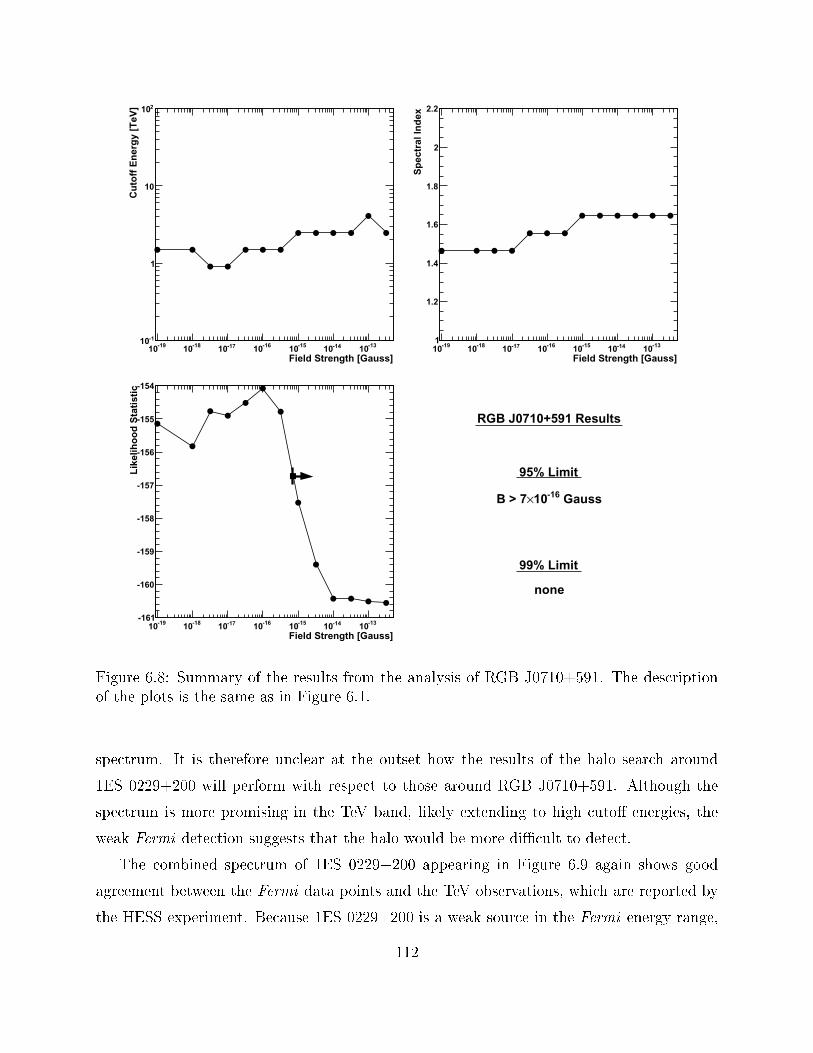
Field Strength [Gauss]-1910 -1810 -1710 -1610 -1510 -1410 -1310

Cu

toff

En

erg

y [T

eV]

-110

1

10

210

Field Strength [Gauss]-1910 -1810 -1710 -1610 -1510 -1410 -1310

Sp

ectr

al In

dex

1

1.2

1.4

1.6

1.8

2

2.2

Field Strength [Gauss]-1910 -1810 -1710 -1610 -1510 -1410 -1310

Lik

elih

oo

d S

tati

stic

-161

-160

-159

-158

-157

-156

-155

-154

RGB J0710+591 Results

95% Limit

Gauss-1610×B > 7

99% Limit

none

Figure 6.8: Summary of the results from the analysis of RGB J0710+591. The des riptionof the plots is the same as in Figure 6.1.spe trum. It is therefore un lear at the outset how the results of the halo sear h around1ES 0229+200 will perform with respe t to those around RGB J0710+591. Although thespe trum is more promising in the TeV band, likely extending to high uto energies, theweak Fermi dete tion suggests that the halo would be more di ult to dete t.The ombined spe trum of 1ES 0229+200 appearing in Figure 6.9 again shows goodagreement between the Fermi data points and the TeV observations, whi h are reported bythe HESS experiment. Be ause 1ES 0229+200 is a weak sour e in the Fermi energy range,112

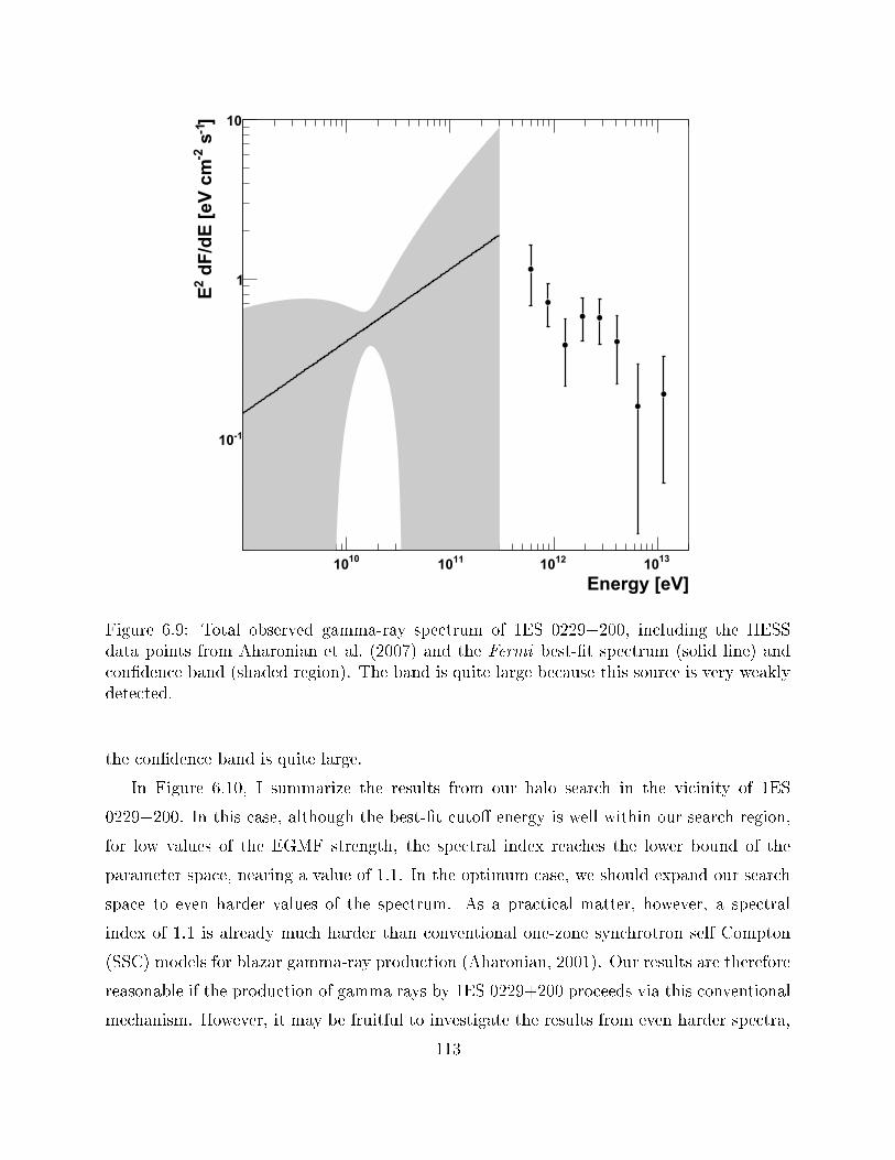
Energy [eV]

1010 1110 1210 1310

]-1

s-2

dF

/dE

[eV

cm

2E

-110

1

10

Figure 6.9: Total observed gamma-ray spe trum of 1ES 0229+200, in luding the HESSdata points from Aharonian et al. (2007) and the Fermi best-t spe trum (solid line) and onden e band (shaded region). The band is quite large be ause this sour e is very weaklydete ted.the onden e band is quite large.In Figure 6.10, I summarize the results from our halo sear h in the vi inity of 1ES0229+200. In this ase, although the best-t uto energy is well within our sear h region,for low values of the EGMF strength, the spe tral index rea hes the lower bound of theparameter spa e, nearing a value of 1.1. In the optimum ase, we should expand our sear hspa e to even harder values of the spe trum. As a pra ti al matter, however, a spe tralindex of 1.1 is already mu h harder than onventional one-zone syn hrotron self Compton(SSC) models for blazar gamma-ray produ tion (Aharonian, 2001). Our results are thereforereasonable if the produ tion of gamma rays by 1ES 0229+200 pro eeds via this onventionalme hanism. However, it may be fruitful to investigate the results from even harder spe tra,113

Field Strength [Gauss]-1910 -1810 -1710 -1610 -1510 -1410 -1310

Cu

toff

En

erg

y [T

eV]

-110

1

10

210

Field Strength [Gauss]-1910 -1810 -1710 -1610 -1510 -1410 -1310

Sp

ectr

al In

dex

1

1.2

1.4

1.6

1.8

2

2.2

Field Strength [Gauss]-1910 -1810 -1710 -1610 -1510 -1410 -1310

Lik

elih

oo

d S

tati

stic

-20

-18

-16

-14

-12

-10

-8

-6

-4

-2

0

1ES 0229+200 Results

95% Limit

Gauss-1610×B > 7

99% Limit

Gauss-1610×B > 3

Figure 6.10: Summary of the results from the analysis of 1ES 0229+200. The des ription ofthe plots is the same as in Figure 6.1.su h as those permitted by the models of Bött her et al. (2008) and Tave hio et al. (2009).I leave this topi for a future study.As shown in Figure 6.10, at 95% onden e we a hieve the same lower limit on theeld strength from 1ES 0229+200 that we did from RGB J0710+591. The results are thennot only onsistent; they also present the optimum situation for a ombination of the twolikelihood statisti urves. Additionally, the urve for 1ES 0229+200 admits a 99% onden elimit of B > 3 × 10−16 Gauss, due to the high onden e of reje tion of the models with114

Field Strength [Gauss]-1910 -1810 -1710 -1610 -1510 -1410 -1310

Lik

elih

oo

d S

tati

stic

-180

-175

-170

-165

-160

-155

Figure 6.11: The ombined likelihood statisti urve from the analysis of RGB J0710+591and 1ES 0229+200.low eld strengths. However, these limits should be onsidered arefully sin e it relies onthe reje tion of spe tral indi es greater than 1.1 on the grounds that they are unphysi al,and this justi ation may not hold up against some less onventional models going beyondthe standard one-zone SSC model, su h as those highlighted by Bött her et al. (2008) andreferen es therein. 6.4.3 Combined LimitBe ause we an multiply likelihoods, it is a straightforward matter to ombine the resultsof Figure 6.8 and Figure 6.10: we simply add the likelihood statisti urves. The summed urve appears in Figure 6.11, from whi h at 95% onden e we derive a robust lower limiton the EGMF strength of B > 3 × 10−15 Gauss. At 99% onden e, this limit be omes115

B > 8 × 10−16 Gauss. Both of the blazars studied in this hapter show eviden e that theexpe ted halo of gamma rays in the energy range a essible to Fermi does not exist. Thiseviden e is strengthened by the ombination of the data from the analysis of ea h blazarindividually.

116

CHAPTER 7STRONG EXTRAGALACTIC MAGNETIC FIELDSThat the EGMF is strong is one possible interpretation of the analysis presented in thisstudy. Certainly it is a ompelling one. While at rst it may seem surprising to nd magneti elds present where there is very little matter, the me hanisms proposed to generate themare based on established physi s. In this hapter, I rst onsider the interpretation of theabsen e of any dete table halo, demonstrated by the analysis presented in this work, as beingdue to the presen e of a strong EGMF. I then on lude with a few remarks on prospe ts forthe future. 7.1 Interpretation of the ResultsThe astrophysi al origin hypothesis, that the EGMF is generated by bulk outows of magne-tized material from radio galaxies (Kronberg, 1994; Kronberg et al., 2001), suers only fromthe di ulty of lling a large fra tion of the universe with magneti elds without inje ting alarge mass along with them. Energeti ally, this pro ess is trivial: the total amount of energyin the EGMF throughout every region in the observable universe is less than the magneti energy ontained in a single luster as long as the EGMF strength is below 10−12 Gauss.However, the bulk transport of plasma into the voids is another matter entirely. Althoughsu h me hanisms ould plausibly produ e the observed intra luster elds, it may indeed bedownright hopeless, as Zweibel (2006) laims, for them to ll the voids. Sin e Dolag et al.(2011) have pointed out that the gamma-ray as ades are sensitive to the dominant ompo-nent of the EGMF in the voids, the astrophysi al origin me hanism may be disfavored bythe dete tion of a strong EGMF. However, it may be possible for these pro esses to operateat earlier times, when the volume of the voids was smaller, or even prior to void formation, ifthere are su ient numbers of a tive or starburst galaxies at z ≈ 6 (Kronberg et al., 1999).Perhaps a more likely andidate for the generation of the EGMF an be found in theprimordial origin hypothesis, in whi h the EGMF is generated during phase transitions inthe early universe. In this s enario, there are two main di ulties. First, the magneti eldmust be generated with strength su ient to avoid being diluted by the universal expansionto a present-day strength lower than the 10−15-Gauss levels suggested by this analysis, while117

still being weak enough not to produ e an observable anisotropi ee t on that expansion.Models over oming this di ulty do exist, although they require a degree of ne tuningto produ e situations amendable to the standard Biermann battery me hanism (Grasso &Rubinstein, 2001), for example. The se ond di ulty is that the EGMF must survive tothe present day without de aying due to magneti diusion. As shown in Figure 1.1, thisrequirement is not parti ularly stringent be ause the range of allowed orrelation lengths isquite broad.If the EGMF is primordial, then its strength is very ompelling in the ontext of mag-neti eld generation due to dierential rotation in galaxies, the α-ω dynamo me hanism.Although the dynamo e ien y is not well known, studies suggest that it an produ e themagneti elds observed in galaxies if the seed EGMFs lie above the very loose lower boundof ∼ 10−30 Gauss (Widrow, 2002). However, due to the existen e of magneti elds dete tedin galaxies at a redshift as distant as z = 2 Bernet et al. (2008), the seed elds may needto be mu h stronger be ause there are only a few y les of gala ti rotation during whi hthe dynamo an operate, due to the limited amount of time sin e galaxy formation. Widrow(2002) notes that the lower bound may be ome mu h more onstraining, falling somewherein the range from 10−16 to 10−10 Gauss. The results of this work, whi h on lude thatthe EGMF may be rather strong, therefore an be taken as eviden e in support of the α-ωdynamo theory of gala ti magneti eld formation.The ultra-high-energy osmi rays (UHECRs), with energies above 1019 eV, are believedto be of extragala ti origin and are therefore inuen ed by the EGMF. In order to dee tthe UHECRs signi antly from their sour es, the EGMF must be relatively strong, possiblyeven stronger than the lower limits suggested in this work. The degree of dee tion isalso related to the orrelation length be ause for smaller orrelation lengths the UHECRs'dire tions undergo a random walk as they ross EGMF domains. However, the same is truefor the ele trons in the as ade, and a smaller orrelation length would imply an even more onstraining lower limit on the eld strength. This limit an be estimated via Equation 4.12.Alternative interpretations of the absen e for the halo also exist. Instrumental systemati errors are one possible explanation for our results. For instan e, we rely on the a ura y ofthe P7SOURCE_V6 model of the instrument response fun tions for the Fermi LAT. If thismodel des ribes a broader PSF than the true PSF of the instrument, the ee ts of the halo ould be obs ured in the likelihood t. Indeed, this exa t problem arose with a previous118

model of the Fermi IRFs, P6_V3, for whi h Ando & Kusenko (2010) laimed a dete tion ofthe EGMF that was later shown to be most likely due to an instrumental ee t (Neronovet al., 2011). The P7SOURCE_V6 model is derived from a tual observations of what areassumed to be point sour es, many of whi h may be blazars. It is possible that the halo ouldbe in orporated into the model, obs uring the true signal. However, this is unlikely providedthat the sour es used in onstru ting the model are predominantly Gala ti sour es andnearby blazars la king a strong TeV omponent. A nalized model of the Fermi LAT basedon both observations and simulations is forth oming. When this new model is available, we an improve the onden e in our results by using it in pla e of the P7SOURCE_V6 model.Our analysis also depends on the assumptions we have made regarding the aring a tivityof the blazar. The IACT observations are likely to be biased be ause the IACTs are morelikely to point toward a blazar if it is determined to be in a aring state. This issue anbe remedied by performing unbiased observations on a sele tion of blazars likely to providegood limits on the EGMF. Dedi ated observations by the existing IACTs or by the futureCherenkov Teles ope Array (CTA) ould a omplish these observations. Additionally, theHigh Altitude Water Cherenkov (HAWC) experiment, whi h will soon be operational, willprovide ontinuous unbiased observations of many blazars now seen by the existing IACTs.A more problemati assumption to over ome is that the blazars have been a tive for aperiod of time su iently long for the as ade to rea h a steady state. If the eld is as strongas 10−15 Gauss, then this time is on the order of 106 years. Observations over this time s aleare presently unavailable and will remain so for the foreseeable future. For this reason, apositive dete tion of the halo would be signi ant be ause it would provide onrmation thatthe blazar engines may be a tive for long periods of time. Sin e su h a positive dete tionappears ina essible to the Fermi instrument, we expe t that the halo may be ome visibleat energies a essible to the IACTs or CTA. However, in these ases, a high uto energy isneeded to ensure that there is substantial as ade in the TeV energy range to produ e a haloin the rst pla e. The trends of in reasing uto energy with eld strength in Figures 6.8and 6.10 are somewhat en ouraging, but sin e the fo us in these gures was on the EGMFstrength, we an make no strong statisti al statements about the true values of the utoenergies. Nevertheless, a sear h for a TeV-s ale halo in the 10−14 to 10−12 Gauss range mayprove fruitful, and indeed ould shed light on the question of the lifetime of blazar engines.Broderi k et al. (2011) have suggested that the absen e of the halo ould be due to the119

development of plasma instabilities in the intera tions between the ele trons and positronsin the as ade and the ele trons in the intergala ti medium (IGM). For parti ularly strongblazars, the ratio of the density in the as ade to the density of the IGM be omes su ientlylarge to trigger plasma instabilities operating on time s ales shorter than the ooling timeof the ele trons via inverse Compton s attering. Su h a pro ess ould dissipate the energyin the as ade into modes in the IGM, ee tively destroying the halo before it has a han eto form. However, the al ulations presented by Broderi k et al. (2011) are dependent onthe extrapolation of results from Bret et al. (2010) to extremely low density ratios, and itis un lear that the plasma approximations still hold. The time s ale over whi h the plasmainstabilities rea h steady state is also un ertain. Regardless, the topi of plasma instabilitiesin the as ade is an intriguing idea that should be explored further in the future.Two other theories have been advan ed that would ompli ate the interpretation of thehalo if it were dete ted. In more onventional terms, Essey & Kusenko (2010) pointed outthat blazars may be sour es of osmi -ray nu lei in the energy range from 1016 to 1019 eV.These osmi rays an intera t with the EBL via the ∆ resonan e, produ ing pions thatde ay to gamma rays at the TeV s ale. Sin e the ross se tion for this intera tion is quitelow, a small number of the osmi rays an intera t nearby Earth, produ ing TeV-s alegamma rays that appear to ome from blazars too distant to be ompatible with even thelower bounds on the EBL. If this pro ess o urs, then the EGMF an be limited from aboveas well as below based on the observations of distant blazars, sin e if the EGMF is toostrong then the osmi rays will be dee ted away from their sour es and the orrelationwith the sour e would be destroyed. It is un lear, however, to what degree the stronger eldsin the LSS ae t the osmi rays' traje tories. Unlike in the ase of the ele tron-positron as ades, whi h are ae ted by the dominant omponent of the EGMF only, the osmi raysare strongly ae ted by all elds along their traje tory, and their passage through a single luster or lament ould be enough to destroy the orrelation with the sour e. Additionally,the total ux of osmi rays observed at Earth an be used to pla e limits on the number ofblazars that generate osmi rays. A detailed study of this ee t has yet to be undertaken.Work by de Angelis et al. (2009) suggests a less onventional theory that the existen eof axion-like parti les (ALPs) ould ontribute to the dete tion of distant blazars. If su hparti les exist, then gamma rays an onvert to ALPs in the magneti eld lo al to the sour eblazar, travel unimpeded by the EBL until they are relatively nearby, and onvert ba k to120

gamma rays in the magneti eld of the Galaxy. While primarily theoreti al, the existen eof ALPs ould ae t the on lusions from our halo sear h, although the pre ise nature oftheir inuen e is presently un lear.Finally, an investigation of the timing information available in the gamma-ray data ouldprovide better limits on the EGMF. Sin e the as ade annot show variability on short times ales, the observed variability in the Fermi energy band must be intrinsi to the sour e.We an set better limits by taking this information into a ount in our ts. Additionally, ifthe EGMF is weak be ause the blazar lifetimes are a tually short, it may prove fruitful tosear h for the hara teristi time delays that are expe ted to follow the ares. As suggestedby Figure 5.25, the dete tion of su h delays ould provide dire t eviden e for an EGMF witha strength below ∼ 10−17 Gauss.7.2 Prospe ts for the FutureThe analysis presented in this work is one of many avenues of resear h available to in reaseour understanding of magneti elds in the universe. There are several ways in whi h it ouldbe improved. As demonstrated in Se tion 6.4.3, the most straightforward way of improvingthe results ould be to ombine the likelihood urves from several blazars. Alternatively,studying an individual blazar whose properties are well measured would eliminate our de-penden e on ertain assumptions about the values of those properties. For instan e, if thebulk Lorentz fa tor or viewing angle an be measured, we an use those values instead ofthe assumptions that we make in this study. Working to hara terize the dependen e of the on lusions on the un ertain lifetime of the blazars ould also prove enlightening, and it maybe possible to make better onstraints by asso iating only steady Fermi measurements withthe as ade.The time is ripe for further investigations into the nature of the EGMF. As mentionedin the previous se tion, there are many avenues of investigation still open to improve ourknowledge of the EGMF and enhan e our understanding of the inner workings of blazars.With new instruments being built to study the TeV sky, and with the existing operationalIACTs and the Fermi LAT, we are living in a golden age of gamma-ray astrophysi s. Itis essential that we make the best use that we an of these opportunities. As we narrowin on a better understanding of what the most extreme existing a elerators an tea h us,121

ultimately we will learn more about the fas inating universe of whi h we are a small part.

122

APPENDIX AEQUATIONS OF MOTION IN COMOVING COORDINATESParti le tra king in a three-dimensional expanding spa e requires a areful sele tion of oor-dinates. We assume an FLRW osmology with a metri spe ied byds2 = c2dt2 −R2(t)d~x2, (A.1)where R(t) is the s ale fa tor at osmi time t. It is onvenient to tra k the parti les interms of the redshift z(t), whi h is dened in terms of the present-day s ale fa tor R(t0) as

1 + z(t) =R(t0)

R(t). (A.2)The onversion between osmi time and redshift is a omplished via the Hubble formula

H(t) =1

R(t)

d

dtR(t) (A.3)by using the equation

dz

dt= −H(z)(1 + z). (A.4)For an FLRW universe, H(z) is given by

H(z) = H0

√

ΩR(1 + z)4 + ΩM (1 + z)3 + ΩΛ + (1 − ΩC)(1 + z)2, (A.5)where ΩR, ΩM , ΩΛ, and ΩC are respe tively the radiation, matter, osmologi al onstant,and urvature densities in units of the riti al density ρC . We assume that the Hubbleparameter H0 is 70 km/s/Mp .A.1 Parti le Dynami sFreely propagating parti les follow geodesi s given byd2xµ

dλ2+ Γ

µνρdxν

dλ

dxρ

dλ= 0, (A.6)123

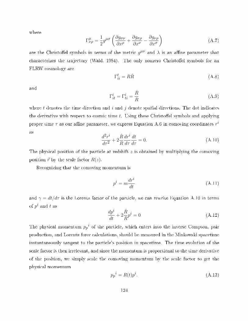
whereΓ

µνρ =

1

2gµσ

(

∂gσν

∂xρ +∂gσρ

∂xν − ∂gνρ

∂xσ

) (A.7)are the Christoel symbols in terms of the metri gµν and λ is an ane parameter that hara terizes the traje tory (Wald, 1984). The only nonzero Christoel symbols for anFLRW osmology areΓt

ii = RR (A.8)andΓi

it = Γiti =

R

R(A.9)where t denotes the time dire tion and i and j denote spatial dire tions. The dot indi atesthe derivative with respe t to osmi time t. Using these Christoel symbols and applyingproper time τ as our ane parameter, we express Equation A.6 in omoving oordinates rias

d2ri

dτ2+ 2

R

R

dri

dτ

dt

dτ= 0. (A.10)The physi al position of the parti le at redshift z is obtained by multiplying the omovingposition ~r by the s ale fa tor R(z).Re ognizing that the omoving momentum is

pi = mdri

dt(A.11)and γ = dt/dτ is the Lorentz fa tor of the parti le, we an rewrite Equation A.10 in termsof pi and t as

dpi

dt+ 2

R

Rpi = 0 (A.12)The physi al momentum pp

i of the parti le, whi h enters into the inverse Compton, pairprodu tion, and Lorentz for e al ulations, should be measured in the Minkowski spa etimeinstantaneously tangent to the parti le's position in spa etime. The time evolution of thes ale fa tor is then irrelevant, and sin e the momentum is proportional to the time derivativeof the position, we simply s ale the omoving momentum by the s ale fa tor to get thephysi al momentumpp

i = R(t)pi. (A.13)124

We then take the time derivative of ppi and use Equation A.12 to getdpp

i

dt= −R

Rpp

i. (A.14)The redshift evolution is then obtained by applying Equation A.4:d

dz~pp =

~pp1 + z

, (A.15)and the solution to this equation gives the familiar expression~pp(z) =

1 + z

1 + z0~pp(z0). (A.16)We arrive at a similar equation for the evolution of the omoving position. If we adopt the onvention to measure distan es in terms of the present-day s ale fa tor, then R(t0) = 1 andby using Equation A.11 in onjun tion with Equation A.13, we nd that

d

dt~r =

c(1 + z)

mc2γ~pp(z) = (1 + z)c~β(z), (A.17)where c~β(z) is the velo ity of the parti le, and with the help of Equation A.4, we obtain

d

dz~r = − c

mc2γH(z)~pp(z) = −c

~β(z)

H(z). (A.18)Although we have derived Equations A.15 and A.18 by using the proper time τ as the aneparameter, the nal equations are independent of τ and are appli able to massless parti lessu h as gamma rays. A.2 Linear MotionSeveral of the Monte Carlo simulation tests des ribed in Se tion 5.1.3 rely on analyti al al ulations of parti le motion in one dimension. These equations are derived in this se tion.To assess the error on the momentum tra king, for instan e, we simply use Equation A.16.Solving Equation A.18 is more di ult, however, be ause of the presen e of H(z). For sim-pli ity, we adopt a onstant-dominated at universe so that H(z) = H0. In one dimension,125

Equation A.18 then be omesdx

dz= −cβ(z)

H0. (A.19)We an express β(z) in terms of the variable q = p0/mc

2, where p0 is the present-daymomentum of the parti le, asβ(z) =

(

1 +1

q2(1 + z)2

)−1/2

. (A.20)In the nonrelativisti limit, q << 1 and Equation A.20 an be approximated byβNR(z) = q(1 + z). (A.21)In this limit the solution to Equation A.19 for a parti le propagating from redshift zi toredshift z is

xNR(z) =qc

2H0

[

(1 + zi)2 − (1 + z)2

]

. (A.22)In the highly relativisti regime, q >> 1 and the approximation for Equation A.20 be omesβHR(z) = 1 − 1

2y2(1 + z)2. (A.23)This alters the solution of Equation A.19 to

xHR(z) =c

H0

[

(zi − z) − 1

2q2

(

1

1 + zi− 1

1 + z

)]

. (A.24)The time delay of as ade parti les relative to a gamma ray that propagates dire tly fromthe sour e may be of interest, for example, for hara terizing the light urves of ares. Thetime for a parti le to propagate a distan e dx along the radial dire tion an be expressed viaEquation A.17 asdt =

dx

cβ(z)(1 + z) cos θ. (A.25)Here, θ is the angle between the parti le's dire tion and the radial dire tion. If the equivalentredshift of the radial gamma ray at the parti le's spa etime position is zr(z), then the timedelay d∆t a quired in propagating through radial distan e dx is the dieren e between dt126

for the parti le and dtr = dx/c(1 + zr) for the radial photon. We an therefore writed∆t

dt=

dxcβ(z)(1+z) cos θ

− dx1+zr(z)

dxcβ(z)(1+z) cos θ

= 1 − cβ(z) cos θ1 + z

1 + zr(z), (A.26)whi h in terms of redshift is

d∆t

dz= − 1

(1 + z)H(z)+

cβ(z) cos θ

(1 + zr(z))H(z). (A.27)In one dimension, cos θ = 1 and the time delay arises solely due to the ee ts of parti le mass.Making this assumption and further simplifying Equation A.27 by assuming a onstant-dominated universe, we arrive at

H0d∆t

dz= − 1

1 + z+

β(z)

1 + zr(z). (A.28)It is evident that we require an expression for zr(z). This we straightforwardly obtain from

dzrdz

=dzrdtr

dtrdt

dt

dz= ((1 + zr)H(zr))

(

cβ(z) cos θ1 + z

1 + zr

)(

− 1

(1 + z)H(z)

)

= −H(zr)

H(z)cβ(z) cos θ.

(A.29)Again working in a onstant-dominated osmology, we nd the ratio of Hubble expressionsdrops out of Equation A.29. The assumption of one-dimensional motion eliminates the cos θ,and in the nonrelativisti limit of Equation A.21 we obtain the solutionzr(z) = zi +

q

2

[

(1 + zi)2 − (1 + z)2

]

. (A.30)By inserting this into Equation A.28 and solving, we ndH0∆t(z) = ln

(

(1 + zi)2

(1 + z)(1 + zy + q2

[

(1 + zi)2 − (1 + z)2]

)

. (A.31)While the Monte Carlo ode expli itly solves Equations A.17 and A.26 via the methodsdes ribed in Se tion 5.1.3, we use the simple ases spe ied by Equations A.24 and A.31 toverify its a ura y. 127

A.3 Ele tromagneti FieldsThe presen e of a magneti eld dee ts harged parti les away from the geodesi of Equa-tion A.6. Following Ja kson (1999) but inverting the sign of his metri to maintain onsis-ten y with the previous se tions, we write the ovariant Lorentz for e equation asdpµdτ

= qFµνdxν

dτ, (A.32)where the ele tromagneti tensor Fµν generalizes in the FLRW osmology to

Fµν = (∂µAν − ΓρµνAρ) − (∂νAµ − Γ

ρνµAρ) = ∂µAν − ∂νAµ, (A.33)and Aν is the ele tromagneti four-potential.The equations of motion are a linear superposition of Equation A.32 with the ovariantgeodesi equation. Starting from Equation A.6, we multiply by gµσ and write

d(gµσpµ)

dτ− pµ

dgµν

dτ+ Γ

µνρp

ν dxρ

dτgµσ = 0. (A.34)Using the vanishing of the metri tensor under the total ovariant derivative, we see that

dgνρ

dτ= gσρΓ

σνµdxµ

dτ+ gνσΓσ

ρµdxµ

dτ, (A.35)and by inserting this into Equation A.34, we nd

dpσdτ

− pµgλσΓλµγdxγ

dτ− pµgµλΓλ

σγdxγ

dτ+ Γ

µνρp

ν dxρ

dτgµσ = 0. (A.36)The se ond and fourth terms in Equation A.36 an el. After renaming dummy indi es, wearrive at the ovariant equations of motion

dpµdτ

= Γρµνpρ

dxν

dτ. (A.37)The total equations of motion are then

dpµdτ

= Γρµνpρ

dxν

dτ+ qFµν

dxν

dτ. (A.38)128

It is now our task to turn Equation A.38 into something useful for parti le tra king.Adopting an FLRW osmology, we start withdpidτ

= RRptdxi

dτ+R

Rpiγ + qFij

dxj

dτ+ qγFit. (A.39)Converting the derivative to osmi time t and rearranging terms gives us

dpidt

= −RRpi +R

Rpi +

q

mγFijp

j + qFit. (A.40)We know that pi = giipi = R2pi, so in terms of the physi al momentum pp

i, we havepi = Rpp

i. Rewriting Equation A.40 in terms of the physi al momentum gives usdpp

i

dt= −R

Rpp

i +q

mγR2Fijpp

j +q

RFit. (A.41)Spe ializing to the ase of no ele tri eld and a onstant omoving magneti eld ~B0 =

R2 ~B(z), we get the nal equation of motiond

dt~pp = −H(z)~pp +

q

mγ~pp × ~B(z). (A.42)

129

APPENDIX BMEAN FREE PATH SAMPLING FOR CONTINUOUS ENERGYLOSSESDue to pro esses su h as redshift that ause propagating parti les to lose energy ontinuously,the mean free path for the parti le at the beginning of its traje tory may be dierent fromthat at the end. For this reason, sampling the intera tion distan e from the original meanfree path may give an in orre t result. I des ribe our solution to this problem in this se tion.In the general ase, the mean free path λ(L) will be a fun tion of the position L of theparti le. The probability of survival for a parti le traveling from position L1 to position L2is thenP (L1 → L2) = exp

(

−∫ L2

L1

dL′

λ(L′)

)

. (B.1)Let λ0 ≤ λ(L) for all L. We make the laim that if we sample an intera tion distan e LI−L1from an assumed mean free path λ0, propagate the parti le from L1 to LI , and ause it tointera t with probability λ0/λ(LI), then the parti le's behavior will fulll Equation B.1 ina statisti al sense. We now seek to demonstrate that this is true.If the sampled position LI is beyond the maximum propagation point L2, then theprobability P0 for survival with 0 han es to intera t is obviouslyP0(L1 → L2) = exp

(

−L2 − L1

λ0

)

, (B.2)whi h fulllsdP0(L1 → L2)

dL2= − 1

λ0exp

(

−L2 − L1

λ0

)

= −P0(L1 → L2)

λ0. (B.3)If the sampled value LI − L1 is less than L2 − L1, then a ording to our pres ription theparti le will survive the intera tion with probability 1 − λ0/λ(LI). We an then write theprobability to survive with one han e to intera t P1 as

dP1(L1 → L2) =

(

−dP0(L1 → LI)

dLIdLI

)(

1 − λ0

λ(LI)

)

P0(LI → L2), (B.4)where the rst term on the right hand side represents the probability that the rst intera tion130

o urs at is LI , the se ond term implements our survival pres ription, and the third term isthe probability for the parti le to survive its propagation from LI to L2 with no additionalintera tions triggered. Repla ing the rst term with the result from Equation B.3 and thethird term with that from Equation B.2 and integrating, we ndP1(L1 → L2) =

∫ L2

L1

dLI

[

exp

(

−LI − L1

λ0

)](

1

λ0− 1

λ(LI)

)

exp

(

−L2 − LI

λ0

)

, (B.5)whi h simplies toP1(L1 → L2) = exp

(

−L2 − L1

λ0

)∫ L2

L1

dLI

(

1

λ0− 1

λ(LI)

)

. (B.6)Taking the derivative of this equation with respe t to L2 gives usdP1(L1 → L2)

dL2= − 1

λ0P1(L1 → L2) + exp

(

−L2 − L1

λ0

)(

1

λ0− 1

λ(L2)

)

, (B.7)and we see from Equation B.2 that this an be expressed asdP1(L1 → L2)

dL2= −P1(L1 → L2)

λ0+P0(L1 → L2)

λ0− P0(L1 → L2)

λ(L2). (B.8)In the general ase, let us assume that we have n+1 andidate positions for intera tions,all of whi h fail to intera t a ording to our pres ription. We an write the dierentialsurvival probability for this ase when the rst intera tion o urs at position LI as

dPn+1(L1 → L2) =

(−dP0(L1 → LI)

dLIdLI

)(

1 − λ0

λ(LI)

)

Pn(LI → L2). (B.9)Integrating to get the total intera tion probability, we ndPn+1(L1 → L2) =

∫ L2

L1

dLI

[

exp

(

−LI − L1

λ0

)](

1

λ0− 1

λ(LI)

)

Pn(LI → L2). (B.10)If we dierentiate Equation B.10 with respe t to L2, there are two terms. One of these isproportional to Pn(L2 → L2), whi h by Equation B.10 vanishes for n > 0. The se ond term131

gives usdPn+1(L1 → L2)

dL2= −

∫ L2

L1

dLI

[

− exp

(

−LI − L1

λ0

)](

1

λ0+

1

λ(LI)

)

×

× dPn(LI → L2)

dL2.

(B.11)Inspired by Equation B.8, let us make the assumption thatdPn(L1 → L2)

dL2= −Pn(L1 → L2)

λ0+Pn−1(L1 → L2)

λ0− Pn−1(L1 → L2)

λ(L2). (B.12)Plugging this into Equation B.11 gives us

dPn+1(L1 → L2)

dL2=

∫ L2

L1

dLI

[

− exp

(

−LI − L1

λ0

)](

1

λ0− 1

λ(LI)

)

×

×(

−Pn(L1 → L2)

λ0+Pn−1(L1 → L2)

λ0− Pn−1(L1 → L2)

λ(L2)

)

.

(B.13)The integrals an be evaluated using Equation B.10, givingdPn+1(L1 → L2)

dL2= −Pn+1(L1 → L2)

λ0+Pn(L1 → L2)

λ0− Pn(L1 → L2)

λ(L2)(B.14)Equation B.12 is therefore valid by indu tion.The total probability of survival with any number of intera tions is

P (L1 → L2) =∞∑

n=0

Pn(L1 → L2). (B.15)Obviously,dP (L1 → L2)

dL2=

∞∑

n=0

dPn(L1 → L2)

dL2. (B.16)We an plug Equation B.12 it into Equation B.16 to get

dP (L1 → L2)

dL2= −

∞∑

n=0

Pn(L1 → L2)

λ0+

∞∑

n=1

Pn−1(L1 → L2)

λ0−

−∞∑

n=1

Pn−1(L1 → L2)

λ(L2).

(B.17)132

The rst and se ond sums in Equation B.17 an el. The third sum over the probability is justthe total probability of surviving given any number of proposed intera tions. Equation B.17therefore redu es todP (L1 → L2)

dL2= −P (L1 → L2)

λ(L2)(B.18)the solution to whi h is Equation B.1. This demonstrates that our pres ription delivers theexpe ted behavior for the parti le.

133

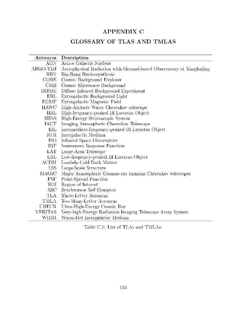
APPENDIX CGLOSSARY OF TLAS AND TMLASA ronym Des riptionAGN A tive Gala ti Nu leusARGO-YBJ Astrophysi al Radiation with Ground-based Observatory at YangbajingBBN Big-Bang Nu leosynthesisCOBE Cosmi Ba kground ExplorerCMB Cosmi Mi rowave Ba kgroundDIRBE Diuse Infrared Ba kground ExperimentEBL Extragala ti Ba kground LightEGMF Extragala ti Magneti FieldHAWC High-Altitude Water Cherenkov teles opeHBL High-frequen y-peaked Bl La ertae Obje tHESS High-Energy Stereos opi SystemIACT Imaging Atmospheri Cherenkov Teles opeIBL Intermediate-frequen y-peaked Bl La ertae Obje tIGM Intergala ti MediumISO Infrared Spa e ObservatoryIRF Instrument Response Fun tionLAT Large-Area Teles opeLBL Low-frequen y-peaked Bl La ertae Obje tΛCDM Lambda Cold Dark MatterLSS Large-S ale Stru tureMAGIC Major Atmospheri Gamma-ray Imaging Cherenkov teles opesPSF Point-Spread Fun tionROI Region of InterestSSC Syn hrotron Self ComptonTLA Three-Letter A ronymTMLA Too-Many-Letter A ronymUHECR Ultra-High-Energy Cosmi RayVERITAS Very-high-Energy Radiation Imaging Teles ope Array SystemWHIM Warm-Hot Intergala ti MediumTable C.1: List of TLAs and TMLAs.

134

REFERENCESA iari, V. A. et al. 2010, ApJ, 715, L49A kermann, M. et al. 2011, ApJ, 743, 171Aharonian, F. et al. 2007, A&A, 475, L9. 2006, A&A, 457, 899Aharonian, F. A. 2001, in International Cosmi Ray Conferen e, Vol. 27, International Cos-mi Ray Conferen e, ed. K.-H. Kampert, G. Heinzelmann, & C. Spiering, I250Aharonian, F. A. 2004, Very high energy osmi gamma radiation : a ru ial window on theextreme Universe, ed. Aharonian, F. A.Aharonian, F. A., Coppi, P. S., & Voelk, H. J. 1994, ApJ, 423, L5Ahlers, M. 2011, Phys. Rev. D, 84, 063006Aielli, G. et al. 2012, Nu lear Instruments and Methods in Physi s Resear h A, 661, 50Ando, S., & Kusenko, A. 2010, ApJ, 722, L39Atkins, R. et al. 2004, ApJ, 608, 680Atwood, W. B. et al. 2009, ApJ, 697, 1071Be k, R. 2008, in Ameri an Institute of Physi s Conferen e Series, Vol. 1085, Ameri anInstitute of Physi s Conferen e Series, ed. F. A. Aharonian, W. Hofmann, & F. Rieger,8396Bernet, M. L., Miniati, F., Lilly, S. J., Kronberg, P. P., & Dessauges-Zavadsky, M. 2008,Nature, 454, 302Biermann, L. 1950, Z. Naturfors h., 5Blasi, P., Burles, S., & Olinto, A. V. 1999, ApJ, 514, L79Blumenthal, G. R., & Gould, R. J. 1970, Reviews of Modern Physi s, 42, 237Bött her, M., Dermer, C. D., & Finke, J. D. 2008, ApJ, 679, L9Bret, A., Gremillet, L., & Die kmann, M. E. 2010, Physi s of Plasmas, 17, 120501Broderi k, A. E., Chang, P., & Pfrommer, C. 2011, ArXiv e-printsBut her, J. C. 2008, Numeri al Methods for Ordinary Dierential Equations, ed. Ja kson,J. D. 135

Bykov, A. M., Paerels, F. B. S., & Petrosian, V. 2008, Spa e S i. Rev., 134, 141Cen, R., & Ostriker, J. P. 1999, ApJ, 514, 1de Angelis, A., Mansutti, O., Persi , M., & Ron adelli, M. 2009, MNRAS, 394, L21Dermer, C. D., Cavadini, M., Razzaque, S., Finke, J. D., Chiang, J., & Lott, B. 2011, ApJ,733, L21Deyoung, T., & et al. 2010, in 38th COSPAR S ienti Assembly, Vol. 38, 2319Dolag, K., Grasso, D., Springel, V., & Tka hev, I. 2005, J. Cosmology Astropart. Phys., 1,9Dolag, K., Ka helrieÿ, M., Ostap henko, S., & Tomàs, R. 2009, ApJ, 703, 1078Dolag, K., Ka helriess, M., Ostap henko, S., & Tomàs, R. 2011, ApJ, 727, L4+Elyiv, A., Neronov, A., & Semikoz, D. V. 2009, Phys. Rev. D, 80, 023010Essey, W., Ando, S., & Kusenko, A. 2011, Astroparti le Physi s, 35, 135Essey, W., & Kusenko, A. 2010, Astroparti le Physi s, 33, 81. 2011, ArXiv e-printsEungwani hayapant, A., & Aharonian, F. 2009, International Journal of Modern Physi s D,18, 911Fegan, D. J. 1997, Journal of Physi s G Nu lear Physi s, 23, 1013Fossati, G., Maras hi, L., Celotti, A., Comastri, A., & Ghisellini, G. 1998, MNRAS, 299,433Fran es hini, A., Rodighiero, G., & Va ari, M. 2008, A&A, 487, 837Gilmore, R. C., Madau, P., Prima k, J. R., Somerville, R. S., & Haardt, F. 2009, MNRAS,399, 1694Gould, R. J., & S hréder, G. P. 1967, Physi al Review, 155, 1408Grasso, D., & Rubinstein, H. R. 2001, Phys. Rep., 348, 163Hanna, D. et al. 2008, Nu lear Instruments and Methods in Physi s Resear h A, 588, 26Hillas, A. M. 1996, Spa e S i. Rev., 75, 17Hovatta, T., Valtaoja, E., Tornikoski, M., & Lähteenmäki, A. 2009, A&A, 494, 527Huan, H., Weisgarber, T., Arlen, T., & Wakely, S. P. 2011, ApJ, 735, L28+136

I hiki, K., Inoue, S., & Takahashi, K. 2008, ApJ, 682, 127Ja kson, J. D. 1999, Classi al Ele trodynami s, ed. Ja kson, J. D.James, F. 2006, Statisti al Methods in Experimental Physi s: 2nd Edition, ed. James, F.(World S ienti Publishing Co)Jau h, J. M., & Rohrli h, F. 1976, The theory of photons and ele trons. The relativisti quantum eld theory of harged parti les with spin one-half, ed. Jau h, J. M. & Rohrli h,F.Jones, F. C. 1968, Physi al Review, 167, 1159Kim, K.-T., Kronberg, P. P., Giovannini, G., & Venturi, T. 1989, Nature, 341, 720Kolb, E. W., & Turner, M. S. 1990, The early universe., ed. Kolb, E. W. & Turner, M. S.Kronberg, P. P. 1994, Reports on Progress in Physi s, 57, 325Kronberg, P. P. 2001, in Ameri an Institute of Physi s Conferen e Series, Vol. 558, Ameri anInstitute of Physi s Conferen e Series, ed. F. A. Aharonian & H. J. Völk, 451462Kronberg, P. P., Dufton, Q. W., Li, H., & Colgate, S. A. 2001, ApJ, 560, 178Kronberg, P. P., Kothes, R., Salter, C. J., & Perillat, P. 2007, ApJ, 659, 267Kronberg, P. P., Les h, H., & Hopp, U. 1999, ApJ, 511, 56Kronberg, P. P., & Perry, J. J. 1982, ApJ, 263, 518Kulsrud, R., Cowley, S. C., Gruzinov, A. V., & Sudan, R. N. 1997a, Phys. Rep., 283, 213Kulsrud, R. M., Cen, R., Ostriker, J. P., & Ryu, D. 1997b, ApJ, 480, 481Kusunose, M., & Takahara, F. 2006, ApJ, 651, 113Li, T., & Ma, Y. 1983, ApJ, 272, 317Mather, J. C. et al. 1994, ApJ, 420, 439Mazin, D., & Raue, M. 2007, A&A, 471, 439MILAGRO Collaboration. 2006, Nu lear Physi s B Pro eedings Supplements, 151, 101Murase, K., Takahashi, K., Inoue, S., I hiki, K., & Nagataki, S. 2008, ApJ, 686, L67Neronov, A., Semikoz, D., Ka helriess, M., Ostap henko, S., & Elyiv, A. 2010, ApJ, 719,L130Neronov, A., & Semikoz, D. V. 2007, JETP Lett., 85, 473137

. 2009, Phys. Rev. D, 80, 123012Neronov, A., Semikoz, D. V., Tinyakov, P. G., & Tka hev, I. I. 2011, A&A, 526, A90Neronov, A., & Vovk, I. 2010, S ien e, 328, 73Pan, D. C., Vogeley, M. S., Hoyle, F., Choi, Y.-Y., & Park, C. 2012, MNRAS, 421, 926Peskin, M. E., & S hroeder, D. V. 1995, An Introdu tion to Quantum Field Theory, ed.Peskin, M. E. & S hroeder, D. V. (Westview Press)Plaga, R. 1995, Nature, 374, 430Protheroe, R. J. 1986, MNRAS, 221, 769Ryu, D., Kang, H., Cho, J., & Das, S. 2008, S ien e, 320, 909Sigl, G., Miniati, F., & Enÿlin, T. A. 2004, Phys. Rev. D, 70, 043007Tave hio, F., Ghisellini, G., Bonnoli, G., & Fos hini, L. 2010a, arXiv:1009.1048Tave hio, F., Ghisellini, G., Fos hini, L., Bonnoli, G., Ghirlanda, G., & Coppi, P. 2010b,MNRAS, 406, L70Tave hio, F., Ghisellini, G., Ghirlanda, G., Costamante, L., & Fran es hini, A. 2009, MN-RAS, 399, L59Taylor, A. M., Vovk, I., & Neronov, A. 2011, A&A, 529, A144The Fermi-LAT Collaboration. 2011, ArXiv e-printsUrry, C. M., & Padovani, P. 1995, PASP, 107, 803Vovk, I., Taylor, A. M., Semikoz, D., & Neronov, A. 2012, ApJ, 747, L14Wald, R. M., ed. 1984, General relativityWeekes, T. C. 1988, Phys. Rep., 160, 1Widrow, L. M. 2002, Reviews of Modern Physi s, 74, 775Zdziarski, A. A. 1988, ApJ, 335, 786Zweibel, E. G. 2006, Astronomis he Na hri hten, 327, 505138