Information retrieval method with shape features extracted by...
70
Information retrieval method with shape features extracted by layered structure representation and its application to shape independent clustering June 2013 Department of Science and Advanced Technology Graduate School of Science and Engineering Saga University CAHYA RAHMAD
Transcript of Information retrieval method with shape features extracted by...

Information retrieval method with shape features
extracted by layered structure representation and
its application to shape independent clustering
June 2013
Department of Science and Advanced
Technology Graduate School of Science and
Engineering Saga University
CAHYA RAHMAD
Information retrieval method with shape features
extracted by layered structure representation and
its application to shape independent clustering
A dissertation submitted to the Department of Science and Advanced Technology,
Graduate School of Science and Engineering, Saga University in partial fulfillment
for the requirements of a Doctorate degree in Information Science
By
CAHYA RAHMAD
Nationality : Indonesianese
Previous degrees : B.S. in Electrical engineering
Faculty of engineering
Brawijaya University, Indonesia
M.S. in Informatics engineering
Graduate School
Tenth of Nopember Institute of Technology, Indonesia
Department of Science and Advanced
Technology Graduate School of Science and
Engineering Saga University
JAPAN
March 2013

APPROVAL
Graduate School of Science and Engineering
Saga University
1 - Honjomachi, Saga 840-8502,
Japan
CERTIFICATE OF APPROVAL
_
Dr.Eng. Dissertation
_
This is to certify that the Dr.Eng. Dissertation of
CAHYA RAHMAD
has been approved by the Examining Committee for the
dissertation requirements for the Doctor of Engineering
degree in Information Science in June 2013.
Dissertation Committee :
Supervisor, Prof. Kohei Arai
Department of Science and Advanced Technology
Member, Prof. Shinichi Tadaki
Department of Science and Advanced Technology
Member, Associate Prof. Hiroshi Okumura
Department of Science and Advanced Technology
Member, Associate Prof. Koichi Nakayama
Department of Science and Advanced Technology

DEDICATION
To my family; my beloved wife: Siti asnipah, All my children(Anggun Audita Alifia
Fatimah, Muhammad Ega Fadhilla Rahmat and Muhammad Aga Febrian Rahmat ), my
parents, my brother and my sister.
i
ABSTRACT
The new method for retrieving image based on shape extraction is proposed for improving the
accuracy. Image retrieval has been used to seek an image over thousand database images. In the
image search engine, the image retrieval has been used for searching an image based on text input
or image. Once an input taking into account, the method will search most related image to the
input. The correlation between input and output has been defined by specific role. we develop the
image retrieval method based on shape features extracted. In conventional method, centroid
contour distance (CCD) is formed by measuring distance between centroid (center) and boundary
of object, however these method cannot capture if an object have multiple boundary in the same
angle.
In this research we proposed new method that able to capture represent of image (feature
vector) although the image have multiple boundary in same angle. Firstly the input image have to
be converted from RGB image to Grayscale image and then follow by edge detection process.
After edge detection process the boundary object will be obtained and then calculate distance
between center of object and the boundary of object and put it in the feature vector and if there is
other boundary on same angle then put it in the different feature vector with different layer or multi
layer centroid contour distance(MLCCD). We applied that method to the simulation dataset and
plankton dataset and the result show that the proposed method better than the conventional method
(CCD, Hsv and Fourier descriptor). We also implement the proposed method with some
modification to cluster a group of data and compare with K-MEAN clustering method and other
clustering method Hierarchical clustering algorithms (Single Linkage, Centroid Linkage,
Complete Linkage and Average Linkage). The experiment result by using the proposed clustering
method show better than K-MEAN and other clustering method.

ii
ACKNOWLEDGEMENTS
This study would not have been possible without the assistances, suggestions and
supports of many individuals and organizations, which I would like to express my deepest
gratitude to them all.
First of all, I would like to thank my supervisor, Prof. Kohei Arai for giving excellent
guidance, useful ideas and patience during my research at Saga University, Japan. As my
teacher and supervisor, Prof. Kohei Arai has given to me a lot of knowledge and research
directions therefore I am able to accomplish my study. This dissertation work could not
complete without his advice, support, guidance and inspiration to conduct my research.
The author is also very grateful to Prof. Shinichi Tadaki, Associate Prof. Hiroshi
Okumura, and Associate Prof. Koichi Nakayama for their help, suggestion and serving as
members of his doctoral program committees. The author is also very grateful to all the
lecturers and staffs of the Chair of Information Science of Saga University for their kind
support and help.
Sincere thanks are due to my colleagues Mr Achmad Basuki, Mr. Tri Harsono, Mr. Lipur
Sugiyanta, Mr. Ronny Mardiyanto, Mr. Tran Sang, Mr. Herman Tolle, Mr Steven
Sentinuwo,Mr. Indra Nugraha Abdullah, Mr. Rosa Andrie Asmara , Mrs Anik Handayani and
all Indonesian student at saga university (Union of Indonesian student), for their help and
encouragement.

iii
I would like to thank the Indonesian Government for awarding me the Dikti scholarship.
This scholarship helps me not only to pursue my study, but it also gives me the opportunity
to know about the Japanese culture, society and new technologies.
Most importantly, I would like to thank my family: the author wishes to express his
love and gratitude to his parents, brother and sister and especially to author’s wife Siti Asnipah,
author’s daughter Anggun Audita Alifia Fatimah also author’s son Muhammad Ega Fadhilla
Rahmat and Muhammad Aga Febrian Rahmat for their patience, sacrifice, support,
understanding, and endless love in authors life among his studies.
Cahya Rahmad
iv
Contents
ABSTRACT ............................................................................................................................. i
ACKNOWLEDGEMENTS .................................................................................................... ii
Contents .................................................................................................................................. iv
List of Figures ......................................................................................................................... vi
List of Tables ........................................................................................................................ viii
1. Introduction ...................................................................................................................... 1
1.1 Information Retrieval ................................................................................................ 1
1.2 Image Retrieval ......................................................................................................... 1
1.3 Motivation and objective .......................................................................................... 3
1.4 Principle of CBIR ..................................................................................................... 3
1.5 Outline of The Thesis................................................................................................ 5
2. Literature Review ............................................................................................................. 7
2.1 Information retrieval ................................................................................................. 7
2.2 Content base image retrieval ..................................................................................... 7
2.2.1 Image ................................................................................................................. 8
2.2.2 Color .................................................................................................................. 8
2.2.3 RGB Color ......................................................................................................... 8
2.2.4 Shape ............................................................................................................... 10
2.2.5 Feature Extraction ............................................................................................ 12
2.2.6 Similarity / Distance Measures ........................................................................ 12
2.3 Clustering ................................................................................................................ 13
2.3.1 Hierarchical Clustering methods ..................................................................... 14
2.3.2 Non-Hierarchical Clustering methods ............................................................. 15
v
2.3.3 Cluster structure ............................................................................................... 16
3. Desain Proposed Method ............................................................................................... 17
3.1 Multi Layer Centroid Contour Distance ................................................................. 17
3.1.1 Shift invariance process ................................................................................... 20
3.1.2 Scale invariance process .................................................................................. 24
3.2 Shape independence Clustering by using layered structure representation ............ 26
4. Experiment and Result ................................................................................................... 28
4.1 Performance Measuring .......................................................................................... 28
4.2 Precision .................................................................................................................. 28
4.3 Recall ...................................................................................................................... 28
4.4 The simulation dataset ............................................................................................ 29
4.5 Experiment with real image .................................................................................... 31
4.6 Clustering Experiment Result ................................................................................. 34
4.7 Result by using layered structure representation .................................................... 35
4.8 Result by using k-mean ........................................................................................... 40
5. Conclusion ...................................................................................................................... 46
References .............................................................................................................................. 47

vi
List of Figures
Figure 1-1. A typical content-based retrieval system .................................................................................................... 4
Figure 1-2. Flow Chart of the Thesis Continuity ........................................................................................................... 6
Figure 2-1 RGB Color Space ........................................................................................................................................ 9
Figure 2-2 HSV Color Space Model............................................................................................................................ 10
Figure 2-3 An apple shape and its centroid distance signature [23] ............................................................................ 11
Figure 2-4 Dendrogram of hierarchical clustering[30] ................................................................................................ 14
Figure 2-5 The numerical example below is given to understand this simple iteration [31] ....................................... 15
Figure 2-6 Examples of condensed clusters (centroids are shown with red dots)[32]. ................................................ 16
Figure 2-7 Examples of shape independent clusters [32] ............................................................................................ 16
Figure 3-1 Diagram block of Proposed Cbir................................................................................................................ 17
Figure 3-2a An object and its Proposed method pattern ............................................................................................ 18
Figure 3-3b An object and its conventional pattern ................................................................................................... 18
Figure 3-4 An simulation data and its Proposed method pattern ................................................................................. 18
Figure 3-5 an object with center and distance ............................................................................................................. 19
Figure 3-6 Example object with its distance and angle ............................................................................................... 21
Figure 3-7 Four Same object with different rotation ................................................................................................... 22
Figure 3-8 Two same object with different scaling ..................................................................................................... 25
Figure 4-1 Example of simulation dataset .................................................................................................................. 29
Figure 4-2 A small portion of phytoplankton image database ..................................................................................... 31
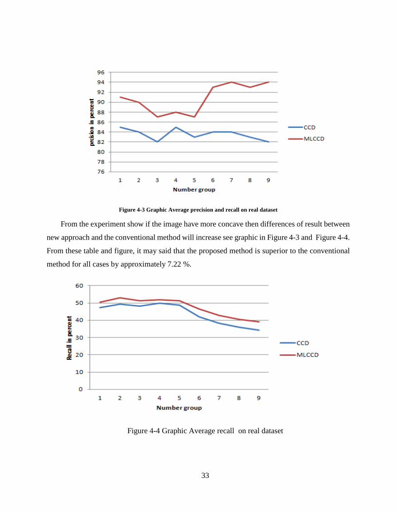
Figure 4-3 Graphic Average precision and recall on real dataset ................................................................................ 33
Figure 4-4 Graphic Average recall on real dataset ..................................................................................................... 33
Figure 4-5 Result by using layered structure representation on the Circular nested dataset ........................................ 35
Figure 4-6 Result by using layered structure representation on the inter related dataset ............................................. 36
Figure 4-7 Result by using layered structure representation on the S shape dataset .................................................... 37
Figure 4-8 Result by using layered structure representation on the u shape dataset .................................................... 37
Figure 4-9 Result by using layered structure representation on the 2 cluster condense dataset .................................. 38

vii
Figure 4-10 Result by using layered structure representation on the 3 cluster condense dataset ................................ 39
Figure 4-11 Result by using layered structure representation on the 4 cluster condense dataset ................................ 39
Figure 4-12 Result by using k-mean on the Circular nested dataset ............................................................................ 40
Figure 4-13 Result by using k-mean on the inter related dataset ................................................................................ 40
Figure 4-14 Result by using k-mean on the S shape dataset ........................................................................................ 41
Figure 4-15 Result by using k-mean on the u shape dataset ........................................................................................ 42
Figure 4-16 Result by using k-mean on the 2 cluster condense dataset ...................................................................... 42
Figure 4-17 Result by using k-mean on the 3 cluster condense dataset ....................................................................... 43
Figure 4-18 Result by using k-mean on the 4 cluster condense dataset ....................................................................... 44

viii
List of Tables
Table 3-1 Feature Vector of object with different rotation .......................................................................................... 23
Table 3-2 Distance between two object with different rotation before shifting process .............................................. 23
Table 3-3 Feature vector of object after shifting process ............................................................................................. 23
Table 3-4 Distance between two object after shifting process ..................................................................................... 24
Table 3-5 Features Vector of object with different scaling before normalization process .......................................... 25
Table 3-6 Distance between two object with different rotation before normalization process .................................... 25
Table 3-7 Features Vector of object with different scaling after normalization process ............................................. 26
Table 3-8 Distance between two object with different rotation after normalization process ....................................... 26
Table 4-1 Average precision on simulation dataset. .................................................................................................... 30
Table 4-2 Average precision on real dataset ................................................................................................................ 32
Table 4-3 Average precision result by using Color (Hsv) and Shape fourier descriptor ............................................. 34
Table 4-4 clustering by using layered structure representation on circular nested dataset .......................................... 35
Table 4-5 clustering by using layered structure representation on inter related dataset .............................................. 36
Table 4-6 clustering by using layered structure representation on S shape dataset ..................................................... 37
Table 4-7 clustering by using layered structure representation on u shape dataset ..................................................... 38
Table 4-8 clustering by using layered structure representation on 2 cluster condense dataset .................................... 38
Table 4-9 clustering by using layered structure representation on 3 cluster condense dataset .................................... 39
Table 4-10 clustering by using layered structure representation on 4 cluster condense dataset .................................. 39
Table 4-11 clustering by using k-mean clustering on circular nested dataset .............................................................. 40
Table 4-12 clustering by using k-mean on inter related dataset .................................................................................. 41
Table 4-13 clustering by using k-mean on S shape dataset ........................................................................................ 41
Table 4-14 clustering by using k-mean on u shape dataset .......................................................................................... 42
Table 4-15 clustering by using k-mean on 2 cluster condense dataset ........................................................................ 43
Table 4-16 clustering by using k-mean on 3 cluster condense dataset ........................................................................ 43
Table 4-17 clustering by using k-mean on 4 cluster condense dataset ........................................................................ 44

ix
Table 4-18 Average error in percent clustering using layered structure representation and
clustering Using k-mean…………………………………………………………………………44

x
List of Abbreviations
IR : Image Retrieval
CBIR : Content Base Image Retrieval
CCD : Centroid Contour Distance
MLCCD : Multi Layer Centroid Contour Distance

1
1. Introduction
This chapter presents the information retrieval, Image retrieval, motivation and objective,
principle of CBIR also outline of the thesis.
1.1 Information Retrieval
In the past decade, With expansion in the multimedia technologies and the Internet, more and
more information has been published in computer readable formats. Big archives of films, music,
images, satellite pictures, books, newspapers and magazines have been made accessible for
computer users. Internet makes it possible for the human to access this huge amount of information.
Information retrieval (IR) is the area of study concerned with searching for documents, for
information within documents, and for metadata about documents, as well as that of searching
relational databases and the World Wide Web. IR is interdisciplinary, based on computer science,
mathematics, library science, information science, information architecture, cognitive psychology,
linguistics, and statistics.
1.2 Image Retrieval
Image retrieval (IR) is system of computer for searching, browsing and retrieving image from
database of digital images. Content based image retrieval(CBIR) also known as query by image
content is technique which uses visual content that well known as features for extracting similar
images from an image in database.
The Content Based Image Retrieval (CBIR) technique uses image content to search and
retrieve digital images. Content-based image retrieval systems were introduced to address the
problems associated with text-based image retrieval. Content based image retrieval is a set of
techniques for retrieving semantically-relevant images from an image database based on
automatically-derived image features.
With expansion in the multimedia technologies and the Internet, CBIR has been an active
research topic since the first 1990’s. The concept of content based retrieval (CBR) in image start
from the first 1980s and Serious applications started in the first 1990s.
2
Retrieval from databases with a large number of images has attracted considerable attention
from the computer vision and pattern recognition society.
Recently every time amount of image in the world are increasing very fast and there is a big
concern to recognize an object in large collections of image databases. Image database every time
become bigger and it make a problem dealing with database organization so the necessity of
efficient algorithm is obvious needed [7][8]. Content Based Image Retrieval (CBIR) is any
technology that in principle helps to organize digital image archives by their visual content [9].
Content base image retrieval or CBIR is a technique for retrieving images that automatically-
derived features such as color, texture and shape. In these case to search an image a user have to
provide query terms such as image file/link or click on some image, and the system will extract
the feature vector and compare it with feature vector in the dataset then return images that similar
to the query. The similarity used for search criteria could be color and texture distribution in images,
region/shape attributes, etc.
Brahmi et al. mentioned the two drawbacks in the keyword annotation image retrieval. First,
images are not always annotated and The manual annotation expensive also time consuming.
Second, human annotation is not objective the same image may be annotated differently by
different observer[10]. Unlike the traditional approach that using the keyword annotation as a
method to search images, CBIR system performs retrieval based on the similarity feature vector
of color, texture, shape and other image content. Comparing to the traditional systems, the CBIR
systems perform retrieval more objectiveness[11].
Global features related to color or texture are commonly used to describe the image content
In image retrieval. The problem using global features is this method cannot capture all parts of
the image having different characteristics[12]. In order to capture specific parts of the image the
local feature is used. On The Content based Image Retrieval (CBIR) local feature of an image is
computed at some point of interest location in order to recognizing an object. In order to recognize
the object firstly the image have to be represented by a feature vector. These feature vector be
converted to different domain to make simple and efficient image characteristic, classification and
indexing[13]. Many techniques to extract the image feature is proposed [8][9][14]. Shape is one
of important visual feature of an image and used to describe image content[15]. One of the shape

3
descriptor is The Centroid contour distance (CCD), it is formed by measuring distance between
centroid (center) and boundary of object[16].
1.3 Motivation and objective
Content-Based Image Retrieval (CBIR) is a technology that helps to search digital image
according to their visual content. This system distinguishes the different regions present in an
image based on their similarity in color, pattern, texture, shape, etc. and decides the similarity
between two images by reckoning the closeness of these different regions.
Research on retrieval systems have been carried out in the media text, image, voice, and video.
With expansion in the multimedia technologies and the Internet, Image retrieval systems is one
technology that is needed in the search for accurate information. The main objective of this thesis
propose a new CBIR system regarding precision and recall. We tried to do some image retrieval
research on low-level features based on color, texture and shape.
1.4 Principle of CBIR
Content-based retrieval uses the contents of images to represent and access the images. A
typical content-based image retrieval system is illustrated in Figure 1.1, in this system there are
tree part. The first part is interface consist Data insertion, Query image and Result display. The
Second part is Query processing consist feature extraction and similarity process. The third part
is feature vector data set and image dataset.
Firstly by using the data insertion some images one by one insert into the system from the data
insertion block go to Feature extraction block. In the feature extraction block, the system
automatically extract visual attributes (color, shape, texture, and spatial information) of each
image based on its pixel values and the result of these process is feature vector.
The feature vector also known as image signature for each of the visual attributes of each
image is very much smaller in size compared to the image data, thus the feature vector contains an
abstraction (compact form) of the images in the image database. One advantage of a signature
over the original pixel values is the significant compression of image representation.

4
However, a more important reason for using the signature is to gain an improved correlation
between image Representation and visual semantics. These feature vector then stores in a feature
vector dataset also the image of these feature vector stores in to image dataset with same index.
Figure 1-1. A typical content-based retrieval system
Secondly by using the query image block, the image as a query pass to the feature vector
block to be extracted then the feature vector of these query image is compared with feature vector
in the feature vector dataset by using similirities process.

5
In these process, retrieval is conducted by applying an indexing scheme to provide an efficient
way of searching the image database. Finally, the system CBIR ranks the search results and then
returns the results that are most similar to the query image throught the result display.
1.5 Outline of The Thesis
This dissertation is organized as five chapters. The structure and relation among chapters are
shown in Figure 1-2.
Chapter 1 This chapter presents the information retrieval, Image retrieval, motivation and
objective, principle of CBIR also outline of the thesis.
Chapter 2 introduces some backgrounds necessary to understand the remainder of the thesis. In
particular, This chapter presents, content base image retrieval, clustering, hierarchical
clustering methods and non-hierarchical clustering methods, cluster structure etc., will
be discussed.
Chapter 3 presents the proposed method, multi layer centroid contour distance, shift invariance
process, Scale invariance process and shape independence clustering
Chapter 4 In this section presents the experiment and result, performance measuring, precision,
recall, The simulation dataset and experiment with real dataset.
Chapter 5 presents conclusion

6
Introduction
Information retrieval
Image retrieval
Motivation and Objective
Principle of CBIROutline of The Thesis
Chapter 1
Experiment and Result
Performance MeasuringPrecisionRecallThe simulation datasetExperiment with real dataset
Chapter 4
Conclusion
Chapter 5
Content base image retrievalClusteringHierarchical Clustering methodsNon-Hierarchical Clusteringcluster structure
Chapter 2
Proposed Method
Multi Layer Centroid Contour DistanceShift invariance processScale invariance processShape independence clustering
Chapter 3
Figure 1-2. Flow Chart of the Thesis Continuity
7
2. Literature Review
This chapter presents the Information retrieval, Content base image retrieval, Clustering,
Hierarchical Clustering methods and Non-Hierarchical Clustering methods.
2.1 Information retrieval
In the past decade, With expansion in the multimedia technologies and the Internet, more and
more information has been published in computer readable formats. Big archives of films, music,
images, satellite pictures, books, newspapers and magazines have been made accessible for
computer users. Information Retrieval is the field of knowledge that deals with the representation,
storage, and access to information items. More specifically, when the retrieved information is a
collection of images, this field of knowledge is called Image Retrieval [17] [18].
2.2 Content base image retrieval
Image retrieval system is a computer system for browsing, searching and retrieving images
from a large database of digital images. The problems of image retrieval are becoming widely
recognized, and the search for solutions an increasingly active area for research and development.
There are three fundamental bases for content based image retrieval i.e. visual feature extraction,
multi-dimensional indexing, and retrieval system design.
Content-based image retrieval (CBIR) is a technique for retrieving images on the basis of
automatically-derived features. The architecture of a CBIR system can be understood as a basic
set of modules that interact within each other to retrieve the database images according to a given
query. Content-based image retrieval, uses the visual contents of an image such as color, shape,
texture, and spatial layout to represent and index the image. In typical content-based image
retrieval systems, the visual contents of the images in the database are extracted and described by
multi-dimensional feature vectors. The feature vectors of the images in the database form a feature
database. To retrieve images, users provide the retrieval system with example images or sketched
figures. The system then changes these examples into its internal representation of feature vectors.
The similarities /distances between the feature vectors of the query example or sketch and those
of the images in the database are then calculated and retrieval is performed with the aid of an

8
indexing scheme. The indexing scheme provides an efficient way to search for the image
database[5].
2.2.1 Image
An image may be defined as a two-dimensional function, f(x, y), where x and y are spatial
(plane) coordinates, and the amplitude at any pair of coordinates (x, y) is called the intensity or
gray level of the image at that point. When x, y, and the amplitude values of fare all finite, discrete
quantities, we call the image a digital image. The field of digital image processing refers to
processing digital images by means of a digital computer. Note that a digital image is com-posed
of a finite number of elements, each of which has a particular location and value. These elements
are referred to as picture elements, image elements and pixels. Pixel is the term most widely used
to denote the elements of a digital image[19].
2.2.2 Color
Color is visual perceptual property corresponding in human to the category called red, green, blue, black,
yellow, etc. Color is produced by spectrum of light that absorbed or reflected then received by the human eye
and processed by the human brain. Color is one of the most widely used features for image similarity
retrieval, Color retrieval yields the best results, in that the computer results of color similarity are
similar to those derived by a human visual system that is capable of differentiating between
infinitely large numbers of colors.
One of the main aspects of color feature extraction is the choice of a color space. A color
space is a multidimensional space in which the different dimensions represent the different
components of color. Mostly color spaces are three dimensional. Example of color space is RGB,
which assigns to each pixel a three element vector giving the color intensities of the three primary
colors, red, green and blue. The space spanned by the R, G and G values completely describes
visible colors, which are represented as vectors in the 3D RGB color spaces.
2.2.3 RGB Color
The RGB model uses three primary colors, red, green and blue, in an additive fashion to be
able to reproduce other colors (see figure 2-1). As this is the basis of most computer displays
today, this model has the advantage of being easy to extract. In a true-color image each pixel will
have has a red, green and blue value ranging from 0 to 255 giving a total of 16777216different

9
colors. Varying levels of the three colors are added to produce more or less any color in the visible
spectrum. This space is device dependent and perceptually non-uniform. This means that a color
relative close together in the RGB space may not necessarily be perceived as being close by the
human eye. RGB space is normally used in Cathode Ray Tube (CRT) monitors, television,
scanners, and digital cameras. For a monitor the phosphor luminescence consists of additive
primaries and we can simply parameterize all colors via the coefficients (α, β, γ), such that C =
αR+βG+γB. The coefficients range from zero (no luminescence) to one (full phosphor output). In
this parameterization the color coordinates fill a cubical volume with vertices black, the three
primaries (red, green, blue), the three secondary mixes (cyan, magenta, yellow), and white as in
figure2-2 [18].
If only the brightness information is needed, color images can be transformed to gray scale
images[20]. The transformation can be made by using equation (see equation 2.1).
Igray=0.3Fr+0.3Fg+0.3Fb (2.1)
But human vision gives more weight to the G channel. The standard conversion to grayscale
mimics the proportion of RGB sensors in the human eye [21] ( see equation 2.2):
Igray =0.3Fr+0.59Fg+0.11Fb (2.2)
Where Fr, Fg and Fb are the intensity of R, G and B component respectively and Igray is the
intensity of equivalent gray level image of RGB image.
Figure 2-1 RGB Color Space
10
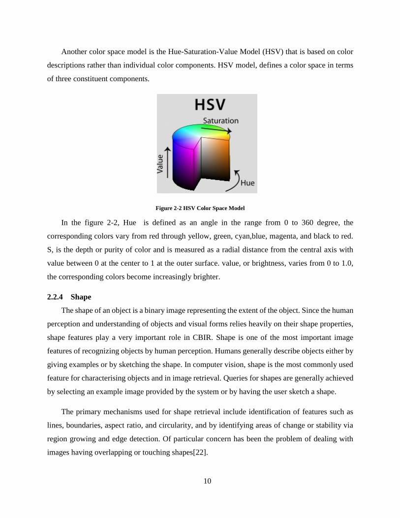
Another color space model is the Hue-Saturation-Value Model (HSV) that is based on color
descriptions rather than individual color components. HSV model, defines a color space in terms
of three constituent components.
Figure 2-2 HSV Color Space Model
In the figure 2-2, Hue is defined as an angle in the range from 0 to 360 degree, the
corresponding colors vary from red through yellow, green, cyan,blue, magenta, and black to red.
S, is the depth or purity of color and is measured as a radial distance from the central axis with
value between 0 at the center to 1 at the outer surface. value, or brightness, varies from 0 to 1.0,
the corresponding colors become increasingly brighter.
2.2.4 Shape
The shape of an object is a binary image representing the extent of the object. Since the human
perception and understanding of objects and visual forms relies heavily on their shape properties,
shape features play a very important role in CBIR. Shape is one of the most important image
features of recognizing objects by human perception. Humans generally describe objects either by
giving examples or by sketching the shape. In computer vision, shape is the most commonly used
feature for characterising objects and in image retrieval. Queries for shapes are generally achieved
by selecting an example image provided by the system or by having the user sketch a shape.
The primary mechanisms used for shape retrieval include identification of features such as
lines, boundaries, aspect ratio, and circularity, and by identifying areas of change or stability via
region growing and edge detection. Of particular concern has been the problem of dealing with
images having overlapping or touching shapes[22].

11
Boundary based shape descriptors have been widely used in image retrieval problems. A
plethora of contour-based descriptors regarding the shape as a 1-D signal sequences, can be found
in literature. Centroid Contour Distance (CCD) as well as Angle Code Histogram (ACH) are well
known and extensively used descriptors.
The (CCD) descriptor is formed by the consecutive boundary-to-centroid distances. Let i be
a shape contour point having (xi, yi) coordinates. Assuming that the shape centroid has coordinates
(xc, yc), the CCD curve is computed for all n boundary points:
CCD(d) = [d1 d2 ... di... dn], d𝑖 = √(x𝑖 − x𝑐)2 + (𝑦𝑖 − 𝑦𝑐)2
Figure 2-3 An apple shape and its centroid distance signature [23]
The distance between two shapes represented by CCD sequences is acquired by calculating
the Euclidean distance of all the rotated versions[7][23][16] (see figure 2-3).
Other shape descriptor is fourier descriptor. The concept of fourier descriptor (FD) has been
widely used in the field of computational shape analysis[24] [25]. The idea of the FD (Fourier
Descriptor) is to use the Fourier transformed boundary as a shape Feature. Suppose A shape
signature z(u) is a 1-D function that represents 2-D areas or boundaries. The discrete Fourier
transform of an signature z(u) is defined as follows:
(2.3)
Where :
n = 0,1,2, … n-1
The coefficients an (n=0,1,..N-1) are called the Fourier descriptors (FDs) of the shape.

12
2.2.5 Feature Extraction
Feature extraction is the process of creating a representation for, or a transformation from the
original data. within the visual feature system, feature can be further classified as general feature
and domain specific features. Feature extraction is the basis of any content-based image retrieval
technique. In a broad sense, features may include both text-based features (key words, annotations)
and visual features (color, texture, shape, etc.). Within the visual feature scope, the features can be
further classified as low-level features and high-level features. The selection of the features to
represent an image is one of the keys of a CBIR system. Because of perception subjectivity and
the complex composition of visual data, there does not exist a single best representation for any
given visual feature [18].
Image feature can be either global or local. A global feature uses the visual features of the
whole image, whereas a local descriptor uses feature of the regions or objects to describe the image
content. To obtain the local feature, an image is often divided into parts first. The simplest way of
dividing an image is to use a partition, which cuts the image into tiles of equal size and shape. A
simple partition does not generate perceptually meaningful regions but is a way of representing
the global features of the image at a finer resolution. A better method is to divide the image into
homogenous regions according to some criterion using region segmentation algorithms that have
been extensively investigated in computer vision.
2.2.6 Similarity / Distance Measures
Instead of exact matching, content-based image retrieval calculates visual similarities between a
query image and images in a database. Accordingly, the retrieval result is not a single image but a
list of images ranked by their similarities with the query image. Many similarity measures have
been developed for image retrieval based on empirical estimates of the distribution of features in
recent years. Different similarity/distance measures will affect retrieval performances of an image
retrieval system significantly[5].
Similarity metric is very important on the retrieval result. One of The similarity measure is
Euclidean distance (See Equation 2.4) between feature representation of image in database image

13
and feature representation of image query. These feature representation of image feature that refer
to the characteristics which describe the contents of an image. The retrieval result is a list of image
ranked by their similarity. Suppose S1 and S2 are shape of object represented multi layer of feature
vectors each (db1, db2,…,dbk) and (qr1, qr2,.....,qrk) then the Distance between S1 and S2 is:
dis(Fdb, Fqr) = √∑(dbj − qrj)2
k
j=1
(2.4)
where :
Fdb = Feature vector of image in database image
Fqr = Feature vector of query image.
k = Number element of feature vector
in these case if the distance between feature representation of image in database image and
feature representation of image query small enough then it to be considered as similar.
2.3 Clustering
Cluster analysis is the process of partitioning data objects (records, documents, etc.) into
meaningful groups or clusters so that objects within a cluster have similar characteristics but are
dissimilar to objects in other clusters. Cluster analysis aims at identifying groups of similar objects
and, therefore helps to discover distribution of patterns and interesting correlations in large data
sets. It has been subject of wide research since it arises in many application domains in engineering,
business and social sciences. Especially, in the last years the availability of huge transactional and
experimental data sets and the arising requirements for data mining created needs for clustering
algorithms that scale and can be applied in diverse domains[26].
Clustering, in data mining, is useful for discovering groups and identifying interesting
distribution in the underlying data. Clustering problem is about partitioning a given data set into
groups (clusters) such that the data points in a cluster are more similar to each other than points in
different clusters [27].
For many years, many clustering algorithms have been proposed and widely used. It can be
divided into two categories, hierarchical and non-hierarchical methods. It is commonly used in
14
many fields, such as data mining, pattern recognition, image classification, biological sciences,
marketing, city-planning, document retrieval, etc. The clustering means process to define a
mapping, f: D → C from some data D={t1, t2, …, tn} to some clusters C={c1, c2,…, cn} based on
similarity between ti [28].
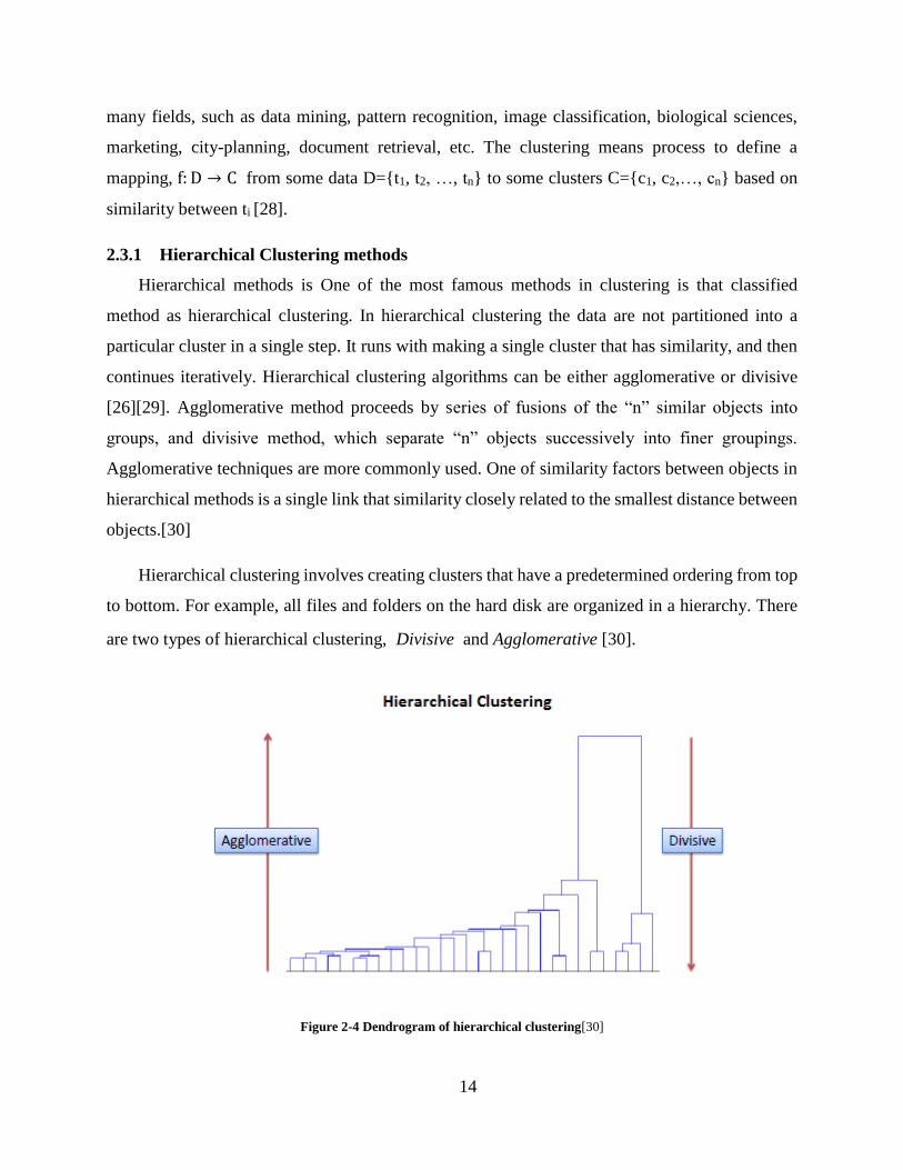
2.3.1 Hierarchical Clustering methods
Hierarchical methods is One of the most famous methods in clustering is that classified
method as hierarchical clustering. In hierarchical clustering the data are not partitioned into a
particular cluster in a single step. It runs with making a single cluster that has similarity, and then
continues iteratively. Hierarchical clustering algorithms can be either agglomerative or divisive
[26][29]. Agglomerative method proceeds by series of fusions of the “n” similar objects into
groups, and divisive method, which separate “n” objects successively into finer groupings.
Agglomerative techniques are more commonly used. One of similarity factors between objects in
hierarchical methods is a single link that similarity closely related to the smallest distance between
objects.[30]
Hierarchical clustering involves creating clusters that have a predetermined ordering from top
to bottom. For example, all files and folders on the hard disk are organized in a hierarchy. There
are two types of hierarchical clustering, Divisive and Agglomerative [30].
Figure 2-4 Dendrogram of hierarchical clustering[30]

15
A. Divisive method
In this method we assign all of the observations to a single cluster and then partition the cluster to two least similar clusters. Finally, we proceed recursively on each cluster until there is one cluster for each observation.
B. Agglomerative method
In this method we assign each observation to its own cluster. Then, compute the similarity (e.g., distance) between each of the clusters and join the two most similar clusters. Finally, repeat steps 2 and 3 until there is only a single cluster left.
2.3.2 Non-Hierarchical Clustering methods
An example of non-hierarchical methods is K-Means Clustering .K-Means Clustering is an
algorithm to classify or to group some objects based on attributes/features into K number of group.
K is positive integer number. The grouping is done by minimizing the sum of squares of distances
between data and the corresponding cluster centroid. Thus, the purpose of K-mean clustering is to
classify the data.
Figure 2-5 The numerical example below is given to understand this simple iteration [31]
The basic step of k-means clustering is simple. In the beginning, we determine number of
cluster K and we assume the centroid or center of these clusters. We can take any random objects

16
as the initial centroids or the first K objects can also serve as the initial centroids. Then the K
means algorithm will do the three steps below until convergence[31].
Iterate until stable (= no object move group):
1. Determine the centroid coordinate
2. Determine the distance of each object to the centroids
3. Group the object based on minimum distance (find the closest centroid)
2.3.3 Cluster structure
The condensed cluster is defined as the cluster members gathered in closely surrounding
locations as is shown in figure 2-5. In the case of condensed cluster, the center of gravity resides
in circle weight of the cluster members. The condensed cluster is very different from the shape
independence cluster that its similar can be seen as such shape patterns. It, in this case, is very
difficult to determine the centroid as illustrated in figure 2-6[32].
Figure 2-6 Examples of condensed clusters (centroids are shown with red dots)[32].
Figure 2-7 Examples of shape independent clusters [32]

17
3. Desain Proposed Method
In this chapter we will describe our proposed method dealing with shape feature extraction by
using multi layer centroid contour distance.
3.1 Multi Layer Centroid Contour Distance
Figure 3.1 is Diagram block of the proposed CBIR.
Input Images from data base image
Preprocessing
Construct feature vector using MLCCD
Input query image
Preprocessing
Construct feature vector using MLCCD
feature vector
Comparison for similarity
Display result base on distance measure
feature vector
Figure 3-1 Diagram block of Proposed Cbir
Firstly images in the database image one by one is extracted. The local feature of an image at
some point at interest location is computed. Interest location of the local feature can be obtained
by converting RGB image to grayscale image and implement the canny filter to detect edge
position then use morphology filter to ensure the shape of object clear. Feature vector is computed
by measuring distance between center of object and point in the boundary object then the result is
placed to the feature vector layer 1 and if the object have other point in the same angle (see Figure
3-2) the result is placed into next layer. All image in the database image is processed by using
same method.

18
Secondly, when a query image is provided then applied same method to obtain feature vector.
These feature vector is compared with other feature vector by using the Euclidean distance.
Figure 3-2a An object and its Proposed method pattern
Figure 3-3b An object and its conventional pattern
Figure 3-4 An simulation data and its Proposed method pattern

19
In figure 3-2a when the angle 0 there is one point have to be captured. However, when the angle
is 270 degree there are three point have to be captured by using MLCCD in these case other
method just capture one point see figure 3-2 b. In Figure 3-3, The object have three point that have
to be captured for all different angle and the result is placed into three layer.
In order to obtain the MLCCD firstly position of the centroid have to be computed (see equation
3.1) then calculate the distance between centroid and the boundary of object repeat this method for
other boundary in same angle and different angle.
Figure 3-5 an object with center and distance
position of the centroid is:
Xc = X1+X2+X3+.… + Xn
n , Yc =
Y1+Y2+Y3+.…+ Yn
n (3.1)
Where:
Xc = position of the centroid in the x axis
Yc = position of the centroid in the y axis
n = Total point in the object (every point have x position and y position)
After the location centroid is founded then calculate the distance between centroid and the
boundary of object by using equation 3.2 repeat this method for other boundary in different angle.
Suppose there are t point in the boundary the distance every point in the boundary with center
is :

20
𝐷𝑖𝑠(𝑛) = √(𝑥(𝑛) − 𝑥𝑐)2 + (𝑦(𝑛) − 𝑦𝑐)2 (3.2)
Where :
n = number point in the boundary( 1,2,..t)
t = total point in the boundary
𝑥𝑐 = position center in the x axis
𝑦𝑐 = position center in the y axis
x(n) = position point number n in the x axis
y(n) = position point number n in the y axis
The computed distances are saved in a vector. In order to achieve rotation invariance and scale
invariance the implementation shifting and normalization to these features vector is needed.
Comparison between two object is conducted by measure distance between two features vector by
using Euclidean distance.
3.1.1 Shift invariance process
In order to achieve rotation invariance the implementation shifting to the features vector is
needed.

21
Figure 3-6 Example object with its distance and angle
In the figure 3-5 distance between center and the boundary of object are 4 at angle 0 degree,
3 at angle 90 degree, 3 at angle 180 degree and 5 at angle 270 degree, however this will change if
the object be rotated. In the figure 3-6 there are 4 object that actually same but different in rotation
around 90 degree and the order of the distance also different.
In the figure 3-6 there are four similar object with different rotation and the distance between
centroid and the boundary also different in same angle. When angle is zero (0) the distance of
object a 4, object b 3, object c 3 and object d 5. When angle 90 the distance object a 3, object b 3,
object c 5 and object d 4. When angle 180 the distance object a 3, object b 5, object c 4 and object
d 3. When angle 270 the distance object a 5, object b 4, object c 3 and object d 3. Base on the
figure 3-5 the feature vector of object a, object b, object c and object d are 4 3 3 5, 3 3 5 4, 3 5 4 3
and 5 4 3 3 as be shown at table 3-1.

22
A
B
C
D
Figure 3-7 Four Same object with different rotation
Table 3-1 is features vector of object A, Object B, object C and object D, Table 3-2 is a distance
between two object in the Table 3-1obtained by using euclidean distance between two features
vector. These distance still high although the objects actually same object that is happened due to
that object is different in rotation.

23
Table 3-1 Feature Vector of object with different rotation
Object Feature Vector
A 4 3 3 5
B 3 3 5 4
C 3 5 4 3
D 5 4 3 3
Table 3-2 Distance between two object with different rotation before shifting process
Object Distance between two object
A-B 2.4495
A-C 3.1623
A-D 2.4495
B-C 2.4495
B-D 3.1623
C-D 2.4495
Table 3-3 is features vector of object A, Object B, object C and object D after shifting process,
In order obtained these value shifting the features vector one by one. In these case there are four
possibility 5433 or 4335 or 3354 or 3543. The highest value is 5433 then choose these value.
Table 3-3 Feature vector of object after shifting process
Object Feature Vector
A 5 4 3 3
B 5 4 3 3
C 5 4 3 3
D 5 4 3 3

24
Table 3-4 a distance between two object at table 3-3 is obtained by using euclidean distance
between two features vector. After shifting process The distance is now become 0.
Table 3-4 Distance between two object after shifting process
Object Distance between two object
A-B 0
A-C 0
A-D 0
B-C 0
B-D 0
C-D 0
3.1.2 Scale invariance process
In order to achieve scale invariance the implementation normalization to the feature vector is
needed.
A

25
B
Figure 3-8 Two same object with different scaling
Figure 3-7 is two same object, object A and object B actually same object with different
scaling and both object have also different features vector as shown in the table 3-5. The distance
between object A and object B is shown in the table 3-6. Although the object A and object B same
object but the distance between them still high.
Table 3-5 Features Vector of object with different scaling before normalization process
Object Feature Vector highest
A 4 3 3 5 5
B 8 6 6 10 10
Table 3-6 Distance between two object with different rotation before normalization process
Object Distance between two object
A-B 7.6811

26
Table 3-7 Features Vector of object with different scaling after normalization process
Object Feature Vector
A 0.8 0.6 0.6 1
B 0.8 0.6 0.6 1
Table 3-8 Distance between two object with different rotation after normalization process
Object Distance between two object
A-B 0
Features vector in the Table 3-7 is obtained from features vector in the table 3-5 devided by
the highest value of its features vector and the feature vector object A and feature vector object B
become same. The table 3-8 shown distance between both object A and object B become 0.
3.2 Shape independence Clustering by using layered structure
representation
In this subsection we implemented the layered structure representation with some
modification to the shape independence clustering.
The algorithm is described as follow:
1. Begin with an assumption that every point “n” is it’s own cluster ci, where i =1,2,…n
2. Calculate the centroid location
3. Calculate the angle and distance for every point
4. Make multi layer centroid contour distance based on step 2 and 3
5. Set i = 1 as initial counter
6. Increment i = i + 1
7. Measure distance between cluster in the location i with cluster in the location i-1 and cluster
27
in the location i+1.
8. Merge two cluster become one cluster base on the closet distance as shown in the step 7
9. Repeat from step 6 to step 8 while i< 360
10. Repeat step 5 to step until the required criteria is met
Firstly in the step 1, let every point “n” is it’s own cluster, if there are n data it mean there
are n cluster. Step 2 obtain the centroid by using equation 3.1 in this case every point have
contribution to find the centroid location. Step 3 Calculate the angle and distance for every point,
the angle is obtained by using arctangent of dy/dx, dy is differences y position between position y
of point in the boundary and y of centroid and dx is differences x position between position x of
point in the boundary and x of centroid. The distance can be obtained by using pythagoras formula.
By using the angle of every point and its distance then make the multi layer centroid contour
distance and set i as counter start from 1 to 360 then calculate distance between every point that
pointed by i on every layer and every point on every layer that pointed i-1 and i+1. After the
distance was calculated then merge two cluster become one cluster base on the closet distance.

28
4. Experiment and Result
In this section, we describe the experiments, using both simulation and real data and then we
verify performance of retrieval by using precision and recall.
4.1 Performance Measuring
In image retrieval contexts, precision and recall are defined in terms of a set of retrieved
image and a set of relevant image. There is two step approach to retrieve the relevant image from
dataset. Firstly, cbir system have to extract a feature vector for every image and put it into feature
dataset. Secondly, The user provide a query image, The cbir system extract its feature vector then
matched with feature vector in the dataset by computing the distances between two feature vector.
The performance of cbir system is calculated by showing image with x top ranking from the
dataset. There is a common way to evaluate the performance of the cbir system such as precision
and recall.
4.2 Precision
Precision measures the retrieval accuracy, it is ratio between the number of relevant images
retrieved and the total number of images retrieved (See equation 4.1).
Precision =NRRI
XR (4.1)
Where :
NRRI = Number of relevant retrieved images
XR = X Top ranking of retrieved images
4.3 Recall
Recall measures the ability of retrieving all relevant images in the dataset. It is ratio between the
number of relevant images retrieved and the whole relevant images in the dataset (See equation
4.2).

29
Recall = NRRI
TR
(4.2)
Where:
NRRI = Number of relevant retrieved images
TR = Total number of relevant images in dataset
4.4 The simulation dataset
The simulation dataset consist combination of curve shape, oval shape, rectangle shape,
Triangle shape, Diamond shape, star shape as shown in Figure 4-1. Also we make these shapes
with different scaling, translation and rotation. Graphic average precision results on simulation
dataset are then shown in Table 4-1.
Figure 4-1 Example of simulation dataset
30
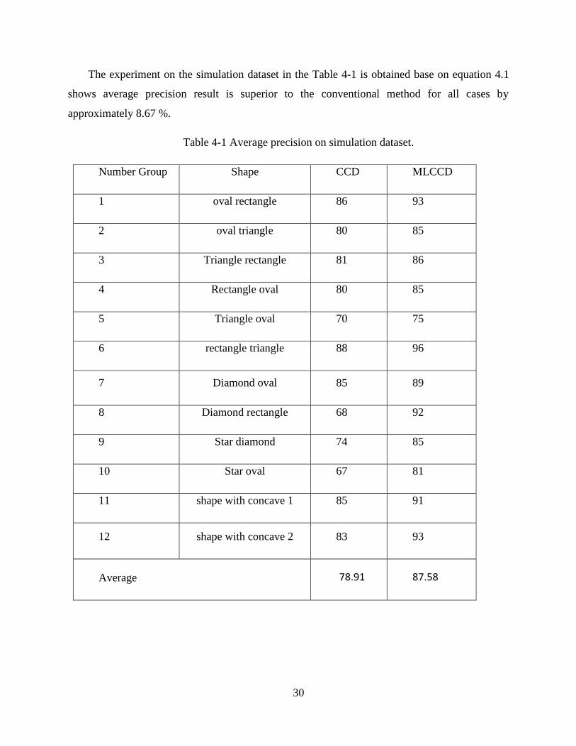
The experiment on the simulation dataset in the Table 4-1 is obtained base on equation 4.1
shows average precision result is superior to the conventional method for all cases by
approximately 8.67 %.
Table 4-1 Average precision on simulation dataset.
Number Group Shape CCD MLCCD
1 oval rectangle 86 93
2 oval triangle 80 85
3 Triangle rectangle 81 86
4 Rectangle oval 80 85
5 Triangle oval 70 75
6 rectangle triangle 88 96
7 Diamond oval 85 89
8 Diamond rectangle 68 92
9 Star diamond 74 85
10 Star oval 67 81
11 shape with concave 1 85 91
12 shape with concave 2 83 93
Average 78.91 87.58
31
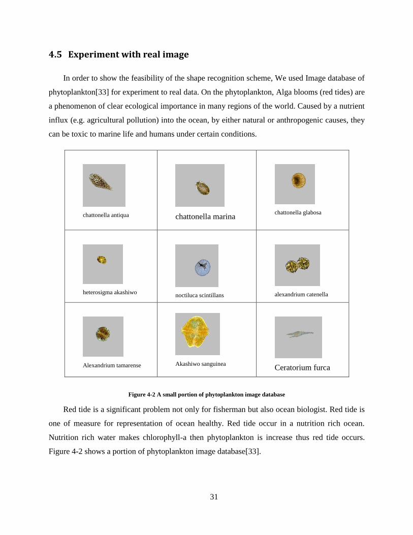
4.5 Experiment with real image
In order to show the feasibility of the shape recognition scheme, We used Image database of
phytoplankton[33] for experiment to real data. On the phytoplankton, Alga blooms (red tides) are
a phenomenon of clear ecological importance in many regions of the world. Caused by a nutrient
influx (e.g. agricultural pollution) into the ocean, by either natural or anthropogenic causes, they
can be toxic to marine life and humans under certain conditions.
chattonella antiqua
chattonella marina
chattonella glabosa
heterosigma akashiwo
noctiluca scintillans
alexandrium catenella
Alexandrium tamarense
Akashiwo sanguinea
Ceratorium furca
Figure 4-2 A small portion of phytoplankton image database
Red tide is a significant problem not only for fisherman but also ocean biologist. Red tide is
one of measure for representation of ocean healthy. Red tide occur in a nutrition rich ocean.
Nutrition rich water makes chlorophyll-a then phytoplankton is increase thus red tide occurs.
Figure 4-2 shows a portion of phytoplankton image database[33].

32
In order to detect red tide, many researcher check phytoplankton in water sampled from the
ocean with microscope. Immediately after they check phytoplankton, they have to identify the
species of phytoplankton. Image retrieval is needed for identification. The proposed method is to
be used for image retrieval and identification.
Table 4-2 Average precision on real dataset
Number
Group
Total
Image Phytoplankton name
precision
Recall
CCD MLCCD CCD
ML
CCD
1 18 chattonella antiqua 85 91 47 50
2 17 chattonella marina 84 90 49 52
3 17 chattonella glabosa 82 87 48 51
4 17 heterosigma
akashiwo 85 88 50 51
5 17 noctiluca scintillans 83 87 48 51
6 20 alexandrium
catenella
84
93 42 46
7 22 Alexandrium
tamarense
84
94 38 42
8 23 Akashiwo
sanguinea
83
93 36 40
9 24 Ceratorium
furca
82
94 34 39
Average 83.5 90.7 43.5 46.8
The experiment on the real dataset in the Table 4-2 is precision measure base on equation 4.1
and recall measure base on equation 4.2. Average precision result by using new approach is higher
3 percent up to 12 percent rather than the coventional method also for average recall result by
using new approach is higher 1 percent up to 5 percent rather than conventional method.
33
Figure 4-3 Graphic Average precision and recall on real dataset
From the experiment show if the image have more concave then differences of result between
new approach and the conventional method will increase see graphic in Figure 4-3 and Figure 4-4.
From these table and figure, it may said that the proposed method is superior to the conventional
method for all cases by approximately 7.22 %.
Figure 4-4 Graphic Average recall on real dataset

34
Table 4-3 Average precision result by using Color (Hsv) and Shape fourier descriptor
Number
Group
Total
Image
Phytoplankton
name
Precision
Color
(HSV)
Fourier
descriptor
1 18 chattonella antiqua 70 85
2 17 chattonella marina 83 86
3 17 chattonella glabosa 81 83
4 17 heterosigma
akashiwo 82 84
5 17 noctiluca scintillans 84 84
6 20 alexandrium
catenella 73 85
7 22 Alexandrium
tamarense
71 84
8 23 Akashiwo
sanguinea 70 85
9 24 Ceratorium
furca 72 83
Average 76.222 84.33
The experiment on the real dataset in the Table 4-3 is precision measure base on equation 4.1.
Average precision result by using color (Hsv) is 76.222 and by using Fourier descriptor is 84.33
the proposed method still have higher result compare these both method.
4.6 Clustering Experiment Result
In order to analyze the accuracy of our proposed method we represent error percentage as
performance measure in the experiment. It is calculated from number of misclassified patterns and

35
the total number of patterns in the data sets[34]. We compare our method with k-means clustering
method to the same dataset.
𝐸𝑟𝑟𝑜𝑟 = 𝑁𝑢𝑚𝑏𝑒𝑟 𝑜𝑓 𝑚𝑖𝑠𝑐𝑙𝑎𝑠𝑠𝑖𝑓𝑖𝑒𝑑
𝑁𝑢𝑚𝑏𝑒𝑟 𝑜𝑓 𝑝𝑎𝑡𝑡𝑒𝑟𝑛 𝑥 100 % (5.1)
The dataset consist Circular nested dataset contain 96 data 3 cluster with cluster1 contain 8
data, cluster 2 contain 32 data and cluster 3 contain 56 data, inter related dataset contain 42 data 2
cluster with cluster 1 contain 21 data and cluster 2 contain 21 data, S shape dataset contain 54 data
3 cluster with cluster1 contain 6 data, cluster 2 contain 6 data and cluster 3 contain 42 data. u shape
dataset contain 38 data 2 cluster with cluster 1 contain 12 data and cluster 2 contain 26 data. The
2 cluster Random dataset contain 34 data 2 cluster with cluster1 contain 15 data and cluster 2
contain 19. The 3 cluster condense dataset contain 47 data 3 cluster with cluster1 contain 16 data,
cluster 2 contain 14 data and cluster 3 contain 17. The last data is 4 cluster condense dataset contain
64 data 4 cluster with cluster1 contain 14 data, cluster 2 contain 18 data cluster 3 contain 15 data
and cluster 4 contain 17 data.
4.7 Result by using layered structure representation
Figure 4-5 Result by using layered structure representation on the Circular nested dataset
In figure 4-5 is Result by using layered structure representation on the Circular nested dataset
and the percentage of error as shown in table 4-3 are 0% for cluster1, 0 % for cluster2 and 0% for
cluster3 average is 0 %.
Table 4-4 clustering by using layered structure representation on circular nested dataset
Cluster Number pattern Misclassified Error in %

36
Cluster1 8 0 0
Cluster2 32 0 0
Cluster3 56 0 0
Average 0
Figure 4-6 Result by using layered structure representation on the inter related dataset
In figure 4-6 is Result by using layered structure representation on the inter related dataset
and the percentage of error as shown in table 4-4 are 0 % for cluster1 and 0 % for cluster2 average
is 0 %.
Table 4-5 clustering by using layered structure representation on inter related dataset
Cluster Number pattern Misclassified Error in %
Cluster1 21 0 0
Cluster2 21 0 0
Average 0

37
Figure 4-7 Result by using layered structure representation on the S shape dataset
In figure 4-7 is Result by using layered structure representation on the S shape dataset and the
percentage of error as shown in table 4-5 are 0 % for cluster1, 0 % for cluster2 and 0% for cluster3
average is 0 %.
Table 4-6 clustering by using layered structure representation on S shape dataset
Cluster Number pattern Misclassified Error in %
Cluster1 6 0 0
Cluster2 6 0 0
Cluster3 42 0 0
Average
Figure 4-8 Result by using layered structure representation on the u shape dataset
In figure 4-8 is Result by using layered structure representation on the u shape dataset and the
percentage of error as shown in table 4-6 are 0 % for cluster1 and 0% for cluster2 average is 0 %.
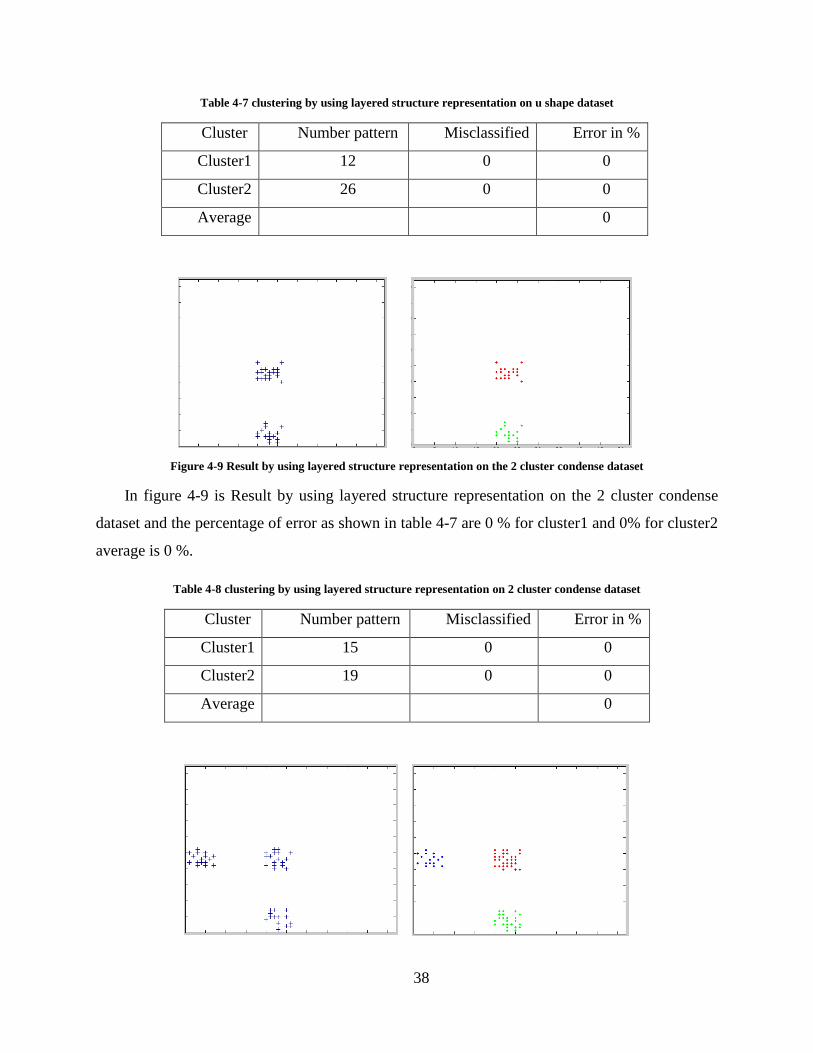
38
Table 4-7 clustering by using layered structure representation on u shape dataset
Cluster Number pattern Misclassified Error in %
Cluster1 12 0 0
Cluster2 26 0 0
Average 0
Figure 4-9 Result by using layered structure representation on the 2 cluster condense dataset
In figure 4-9 is Result by using layered structure representation on the 2 cluster condense
dataset and the percentage of error as shown in table 4-7 are 0 % for cluster1 and 0% for cluster2
average is 0 %.
Table 4-8 clustering by using layered structure representation on 2 cluster condense dataset
Cluster Number pattern Misclassified Error in %
Cluster1 15 0 0
Cluster2 19 0 0
Average 0
39
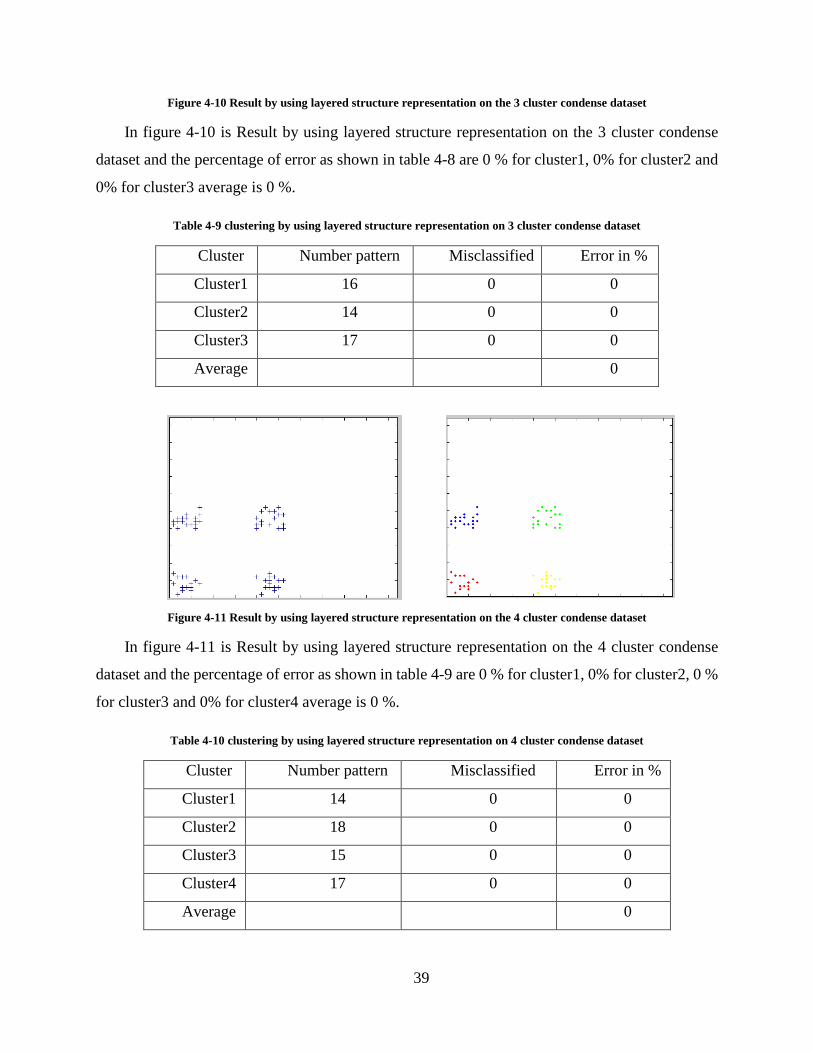
Figure 4-10 Result by using layered structure representation on the 3 cluster condense dataset
In figure 4-10 is Result by using layered structure representation on the 3 cluster condense
dataset and the percentage of error as shown in table 4-8 are 0 % for cluster1, 0% for cluster2 and
0% for cluster3 average is 0 %.
Table 4-9 clustering by using layered structure representation on 3 cluster condense dataset
Cluster Number pattern Misclassified Error in %
Cluster1 16 0 0
Cluster2 14 0 0
Cluster3 17 0 0
Average 0
Figure 4-11 Result by using layered structure representation on the 4 cluster condense dataset
In figure 4-11 is Result by using layered structure representation on the 4 cluster condense
dataset and the percentage of error as shown in table 4-9 are 0 % for cluster1, 0% for cluster2, 0 %
for cluster3 and 0% for cluster4 average is 0 %.
Table 4-10 clustering by using layered structure representation on 4 cluster condense dataset
Cluster Number pattern Misclassified Error in %
Cluster1 14 0 0
Cluster2 18 0 0
Cluster3 15 0 0
Cluster4 17 0 0
Average 0

40
4.8 Result by using k-mean
Figure 4-12 Result by using k-mean on the Circular nested dataset
In figure 4-12 is Result by using k-mean on the Circular nested dataset and the percentage of
error as shown in table 4-10 are 50% for cluster1, 90.625% for cluster2 and 62.5% for cluster3
average is 67.7 %.
Table 4-11 clustering by using k-mean clustering on circular nested dataset
cluster Number pattern Misclassified Error in %
Cluster1 8 4 50
Cluster2 32 29 90.625
Cluster3 56 35 62.5
Average 67.7
Figure 4-13 Result by using k-mean on the inter related dataset

41
In figure 4-13 is Result by using k-mean on the inter related dataset and the percentage of
error as shown in table 4-11 are 19.04% for cluster1 and 19.04% for cluster2 average is 19.04 %.
Table 4-12 clustering by using k-mean on inter related dataset
Cluster Number pattern Misclassified Error in %
Cluster1 21 4 19.04
Cluster2 21 4 19.04
Average 19.04
Figure 4-14 Result by using k-mean on the S shape dataset
In figure 4-14 is Result by using k-mean on the S shape dataset and the percentage of error as
shown in table 4-12 are 0% for cluster1, 0% for cluster2 and 69.04% for cluster3 average is
23.01 %.
Table 4-13 clustering by using k-mean on S shape dataset
Cluster Number pattern Misclassified Error in %
Cluster1 6 0 0
Cluster2 6 0 0
Cluster3 42 29 69.04
Average 23.01

42
Figure 4-15 Result by using k-mean on the u shape dataset
In figure 4-15 is Result by using k-mean on the u shape dataset and the percentage of error as
shown in table 4-13 are 25% for cluster1 and 42.30% for cluster2 average is 33.65 %.
Table 4-14 clustering by using k-mean on u shape dataset
Cluster Number pattern Misclassified Error in %
Cluster1 12 3 25
Cluster2 26 11 42.30
Average 33.65
Figure 4-16 Result by using k-mean on the 2 cluster condense dataset
In figure 4-16 is Result by using k-mean on the 2 cluster condense dataset and the percentage
of error as shown in table 4-14 are 0% for cluster1 and 0% for cluster2 average is 0 %.

43
Table 4-15 clustering by using k-mean on 2 cluster condense dataset
Cluster Number pattern Misclassified Error in %
Cluster1 15 0 0
Cluster2 19 0 0
Average 0
Figure 4-17 Result by using k-mean on the 3 cluster condense dataset
In figure 4-17 is Result by using k-mean on the 3 cluster condense dataset and the percentage
of error as shown in table 4-15 are 0% for cluster1, 0% for cluster2 and 0% for cluster3 average is
0 %.
Table 4-16 clustering by using k-mean on 3 cluster condense dataset
Cluster Number pattern Misclassified Error in %
Cluster1 16 0 0
Cluster2 14 0 0
Cluster3 17 0 0
Average 0

44
Figure 4-18 Result by using k-mean on the 4 cluster condense dataset
In figure 4-18 is Result by using k-mean on the 4 cluster condense dataset and the percentage
of error as shown in table 4-16 are 0% for cluster1, 0% for cluster2, 0% for cluster3 and 0% for
cluster4 average is 0 %.
Table 4-17 clustering by using k-mean on 4 cluster condense dataset
Cluster Number pattern Misclassified Error in %
Cluster1 14 0 0
Cluster2 18 0 0
Cluster3 15 0 0
Cluster4 17 0 0
Average 0
Table 4-17 is Average error in percent clustering using layered structure representation and
clustering using k-mean show average error clustering using layered structure representation 0 %
and average misclassified clustering using k-mean 20.48%.
Table 4-18 Average error in percent clustering using layered structure representation and clustering Using k-mean
Dataset Using layered structure
representation Error in %
Using k-mean
Error in %
Circular nested 0 67.7
inter related 0 19.04
S shape 0 23.01
u shape 0 33.65
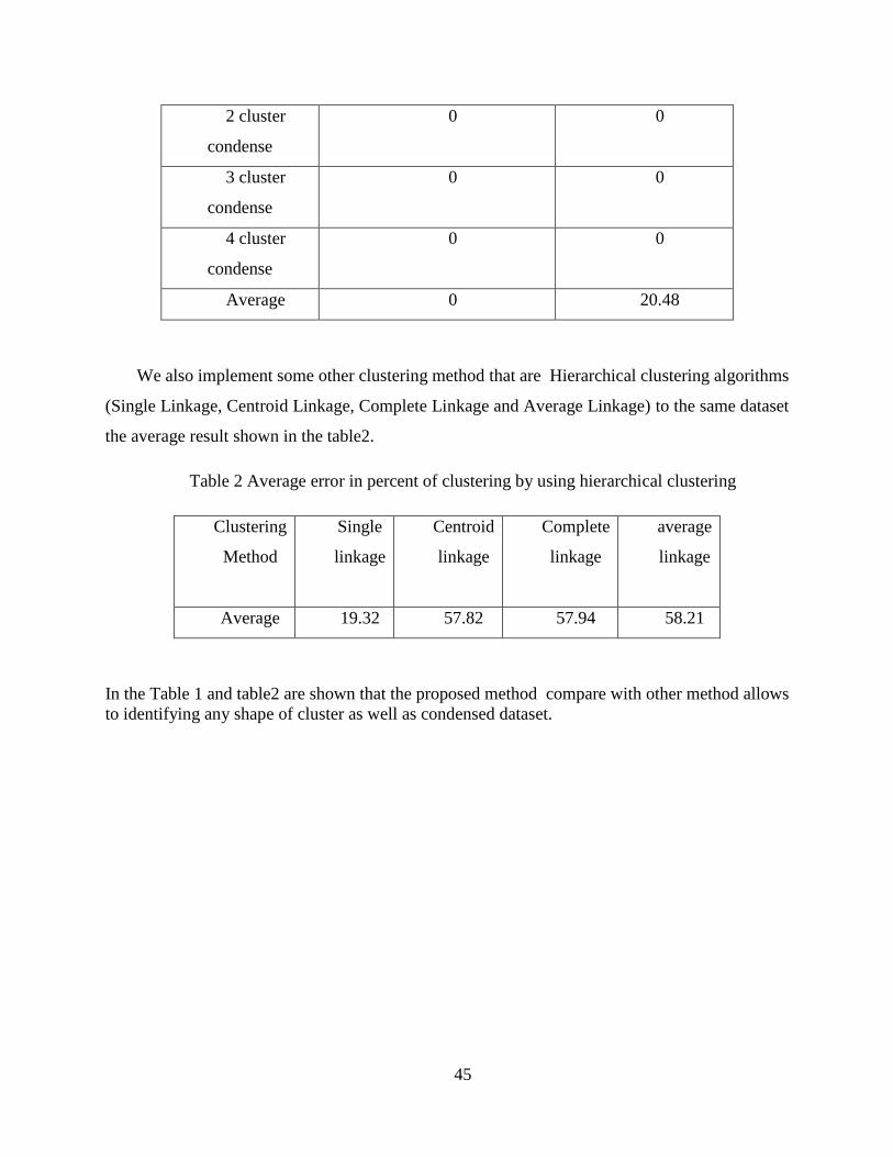
45
2 cluster
condense
0 0
3 cluster
condense
0 0
4 cluster
condense
0 0
Average 0 20.48
We also implement some other clustering method that are Hierarchical clustering algorithms
(Single Linkage, Centroid Linkage, Complete Linkage and Average Linkage) to the same dataset
the average result shown in the table2.
Table 2 Average error in percent of clustering by using hierarchical clustering
Clustering
Method
Single
linkage
Centroid
linkage
Complete
linkage
average
linkage
Average 19.32 57.82 57.94 58.21
In the Table 1 and table2 are shown that the proposed method compare with other method allows
to identifying any shape of cluster as well as condensed dataset.

46
5. Conclusion
A shape feature based multi layer centroid contour distance has been implemented. In this
research, we propose a new approach to extract features of an object shape that has some points
with the same angle. In the conventional method if there is multiple point in same angle just capture
one point that nearest to the centroid and placed it into one layer. While using the proposed method
if there is multiple point in the same angle all point will be captured and the result be placed into
multiple vector layers.
The experiment results on simulated data demonstrate a new approach has the advantage of
8.67 percent higher than using conventional method. Precision results on real data (real data on
phytoplankton dataset) with a new approach has also the advantage of 7.22 percent higher than
using conventional method. We applied that method to the simulation dataset and plankton dataset
and the result show that the proposed method better than the conventional method (CCD, Hsv and
Fourier descriptor).
We also implement the proposed method with some modification to cluster a group of data
and compare with K-MEAN clustering method and other clustering method. The experiment result
by using the proposed clustering method show better than K-MEAN and hierarchical clustering
(Single linkage, Centroid Linkage, Complete linkage and average linkage)

47
References
[1] K. Jung, K. In Kim, and A. K. Jain, “Text information extraction in images and video: a
survey,” Pattern Recognition, vol. 37, no. 5, pp. 977–997, May 2004.
[2] P. B. Thawari and N. J. Janwe, “CBIR BASED ON COLOR AND TEXTURE,” vol. 4,
no. 1, pp. 129–132, 2011.
[3] C. Carson and S. Belongie, “Blobworld: Image segmentation using expectation-
maximization and its application to image querying,” Pattern Analysis and …, 2002.
[4] R. Datta, D. Joshi, J. Li, and J. Z. Wang, “Image retrieval: Ideas, influences, and trends of
the new age,” ACM Computing Surveys, vol. 40, no. 2, pp. 1–60, Apr. 2008.
[5] F. Long, H. Zhang, and D. Feng, “Fundamentals of content based image retrieval,”
“Multimedia Information Retrieval and Management. Technological Fundamentals and
Applications,”Multimedia Signal Processing Book, Chapter 1, Springer-Verlag, Berlin
Heidelberg New York, pp. 1–26, 2003.
[6] H. Müller and A. Geissbuhler, “Benchmarking image retrieval applications,” Proc. of the
10th Intern. …, 2004.
[7] FotopoulouF and EconomouG, “Multivariate angle scale descriptor of shape retrieval,”
Proc. Signal. Process Appl. Math. Electron …, pp. 105–108, 2011.
[8] Y. Liu, D. Zhang, G. Lu, and W.-Y. Ma, “A survey of content-based image retrieval with
high-level semantics,” Pattern Recognition, vol. 40, no. 1, pp. 262–282, Jan. 2007.
[9] N. Singhai and S. K. Shandilya, “A Survey On: Content Based Image Retrieval Systems,”
International Journal of Computer Applications, vol. 4, no. 2.
[10] M. Kherfi, Brahmi, and Ziou, “Combining Visual Features with Semantics for a More
Effective Image Retrieval,” in in ICPR ’04, vol. 2,, 12012BC, pp. 961–964.
[11] H. Yu, M. Li., Zhang, and Feng, “Color texture moments for content-based image
retrieval,” in In International Conference on Image Processing, 2002, pp. 24–28.
[12] N. Sebe, Q. Tian, E. Loupias, Lew, and Huang, “Evaluation of salient point techniques,”
Image and Vision Computing, vol. 21, no. 13–14, pp. 1087–1095, Dec. 2003.
[13] J.-R. Ohm, F. Bunjamin, W. Liebsch, B. Makai, K. Müller, a. Smolic, and D. Zier, “A set
of visual feature descriptors and their combination in a low-level description scheme,”
Signal Processing: Image Communication, vol. 16, no. 1–2, pp. 157–179, Sep. 2000.
48
[14] D. Zhang and G. Lu, “A Comparative Study of Three Region Shape Descriptors,” no.
January, pp. 1–6, 2002.
[15] K. Arai and C. Rahmad, “Content Based Image Retrieval by using Multi Layer Centroid
Contour Distance,” vol. 2, no. 3, pp. 16–20, 2013.
[16] S. C.Chang, S. Hwang, and D.Buehrer, “A Shape recognition scheme based on relative
distance of feature points from the centroid,” Pattern Recognition, vol. 11, pp. 1053–1063,
1991.
[17] “Blaser, A. 1979. Database Techniques for Pictorial Applications, Lecture Notes in
Computer Science, Springer Verlag GmbH. 81.”
[18] A. Khokher and R. Talwar, “Content-based Image Retrieval: Feature Extraction
Techniques and Applications,” International Conference on Recent Advances and Future
Trends in Information Technology (iRAFIT2012) proceedings published in International
Journal of Computer Applications® (IJCA) 9, 2012.
[19] R. C. Gonzalez and R. E. Woods, Digital Image Processing, Second Edi. Tom Robbins,
2001.
[20] G. D. Finlayson, G. Qiu, and M. Qiu, “Contrast Maximizing and Brightness Preserving
Color to Grayscale Image Conversion,” 1999.
[21] “http://www.math.ucla.edu/~wittman/10c.1.11s/Lectures/Lec24.pdf.” .
[22] A. A. Goodrum, “Image Information Retrieval : An Overview of Current Research,” vol.
3, no. Special issue on information science research, 2000.
[23] D. Zhang and G. Lu, “Review of shape representation and description techniques,”
Pattern Recognition, vol. 37, no. 1, pp. 1–19, Jan. 2004.
[24] FUNTOURA Costa and C. R. M., “Shape Analysis and Classifica tion: Theory and
Practice,” Boca Raton, FL.: CRC Press, 2001.
[25] G. E. Q. Jeffrey, “Fourier Descriptors with Different Shape Signatures : a Comparative
Study for å,” vol. 47, no. 50728503, 2011.
[26] M. Halkidi, “On Clustering Validation Techniques,” Journal of Intelligent Information
Systems, pp. 107–145, 2001.
[27] S. Guha, R. Rastogi, and K. Shim, “CURE: An Efficient Clustering algorithm for Large
Databases,” in SIGMOD ’98 Proceedings of the 1998 ACM SIGMOD international
conference on Management of data, 1998, pp. 73–84.
49
[28] K. Arai and A. R. Barakbah, “Cluster construction method based on global optimum
cluster determination with the newly defined moving variance,” vol. 36, no. 1, pp. 9–15,
2007.
[29] D. Frossyniotis, a. Likas, and a. Stafylopatis, “A clustering method based on boosting,”
Pattern Recognition Letters, vol. 25, no. 6, pp. 641–654, Apr. 2004.
[30] “http://www.saedsayad.com/clustering_hierarchical.htm.” .
[31] K. Teknomo, “K-Means Clustering Tutorial,” Medicine, pp. 1–12, 2006.
[32] K. Arai and A. R. Barakbah, “Automatic shape independent clustering with global
optimum cluster determinations By,” vol. 36, no. 1, pp. 1–6, 2007.
[33] “Kohei Arai and Yasunori Terayama, Polarized radiance from red tide, Proceedings of the
SPIE Asia Pacific Remote Sensing, AE10-AE101-14, Invited Paper, 2010.”
[34] K. Arai and A. Ridho, “Hierarchical K-means: an algorithm for centroids initialization for
K-means,” vol. 36, no. 1, pp. 25–31, 2007.

50
Appendix
Shape is one of the primary features in Content Based Image Retrieval (CBIR). Shape is also
one of important visual feature of an image and used to describe image content. The shape of an
object is a binary image representing the extent of the object.
Since the human perception and understanding of objects and visual forms relies heavily on
their shape properties, shape features play a very important role in CBIR. Shape is one of the most
important image features of recognizing objects by human perception.
The algorithm of A shape features extracted by layered structure representation is described
as follow:
1. Input image from database image / Query Image
2. Convert RGB image To Gray Image
3. Edge detection
4. Morphology Filter
5. Construct feature vector using multi layer centroid contour distance (MLCCD)
6. Comparison for similarity retrieval
7. Display Result based on distance measure
Image from database image or from query image convert from RGB image into Gray scale
image then implement the canny filter to detect edge position then use morphology filter to ensure
the shape of object clear. Then local feature of an image at some point at interest location is
computed.
Feature vector is computed by measuring distance between center of object and point in the
boundary object Then the result is placed to the feature vector layer by layer and then the feature
vector that obtained from database image and Query Image be compared each other (similarity
process) then display the result.
The retrieval result is not a single image but a list of image ranked by their similarity. in these
case if the distance between feature representation of image in database image and feature
representation of image query small enough then it to be considered as similar.

51
Centroid position :
Xc = X1+X2+X3+.… + Xn
n , Yc =
Y1+Y2+Y3+.…+ Yn
n
Xc is position of the centroid in the x axis and Yc is position of the centroid in the y axis and
n is Total point in the object .
Distance between centroid and boundary of shape :
𝐷𝑖𝑠(𝑛) = √(𝑥(𝑛) − 𝑥𝑐)2 + (𝑦(𝑛) − 𝑦𝑐)2
n is number point in the boundary of object ( 1,2,..t), t is total point in the boundary, 𝑥𝑐 is
position center in the x axis, 𝑦𝑐 is position center in the y axis, x(n) is position point number n in
the x axis and y(n) is position point number n in the y axis.
The computed distances are saved in a vector layer by layer. The next layer will happen if there
are more than one point in the boundary with same angle.
In order to achieve rotation invariance, scale invariance and translation invariance
implementation shifting and normalization to these vector is needed. The rotation invariance can
be obtained by shifting the feature vector, the biggest value shift to the left side. The scale
invariance can be obtained with all feature vector divided by the highest value. The translation
invariance can be obtained after the centroid location found.
Cluster analysis is the process of partitioning data objects (records, documents, etc.) into
meaningful groups or clusters so that objects within a cluster have similar characteristics but are
dissimilar to objects in other clusters. Cluster analysis aims at identifying groups of similar objects
and, therefore helps to discover distribution of patterns and interesting correlations in large data
sets. Cluster: a collection of data objects. Similar to one another within the same cluster; Dissimilar
to the objects in other clusters. Some example of clustering are K-Mean Clustering, Single linkage
clustering, Centroid linkage clustering, Complete linkage clustering and Average linkage
clustering.

52
K-Mean Clustering
K-Means Clustering is an algorithm to classify or to group some objects based on
attributes/features into K number of group. K is positive integer number. The grouping is done by
minimizing the sum of squares of distances between data and the corresponding cluster centroid.
Thus, the purpose of K-mean clustering is to classify the data.
The basic step of k-means clustering is simple. In the beginning, we determine number of
cluster K and we assume the centroid or center of these clusters. We can take any random objects
as the initial centroids or the first K objects can also serve as the initial centroids. Then the K
means algorithm will do the three steps below until convergence.
The algorithm k-means clustering
1. Determine number of cluster K then choose randomly the object to the cluster
2. Determine the centroid coordinate
3. Determine the distance of each object to the centroids
4. Group the object based on minimum distance (find the closest centroid)
5. Iterate step 2 ,3 and 4 until stable ( no object move to other group)
Single linkage clustering, Centroid linkage clustering, Complete linkage clustering and
Average linkage clustering are Hierarchical methods. The Hierarchical methods is One of the most
famous methods in clustering is that classified method as hierarchical clustering.
In hierarchical clustering the data are not partitioned into a particular cluster in a single step.
It runs with making a single cluster that has similarity, and then continues iteratively. Hierarchical
clustering algorithms can be either agglomerative or divisive.
The agglomerative method proceeds by series of fusions of the “n” similar objects into groups,
and divisive method, which separate “n” objects successively into finer groupings. The
Agglomerative method they produce a sequence of clustering schemes of decreasing number of
clusters at each step. The clustering scheme produced at each step results from the previous one
by merging the two closest clusters into one cluster.
The divisive algorithms. These algorithms produce a sequence of clustering schemes
increasing the number of clusters at each step. Contrary to the agglomerative algorithms the

53
clustering produce at each step results from the previous one by splitting a cluster into two cluster.
Agglomerative techniques are more commonly used.
Hierarchical clustering proceeds successively by either merging smaller cluster into larger
ones, or by splitting larger clusters. The result of the algorithm is a tree of clusters, called
dendogram, which shows how the clusters are related. By cutting the dendogram at a desire level,
a clustering of the data items into disjoint groups is obtained.
Basic algorithm Most popular hierarchical clustering technique is
1. Compute the distance matrix between the input data points
2. Let each data point be a cluster
3. Repeat
4. Merge the two closest clusters
5. Update the distance matrix
6. Until only a single cluster remains
Distance between two clusters
Single-link distance between clusters Ci and Cj is the minimum distance between any object
in Ci and any object in Cj The similarity is based on closely related to the smallest distance between
objects at two cluster.
The distance is defined by the two most similar objects
jiyxjisl CyCxyxdCCD ,),(min, ,
Centroid link distance between clusters Ci and Cj is the distance between the centroid ri of Ci
and the centroid rj of Cj.
),(, jijicentroids rrdCCD
Complete-link distance between clusters Ci and Cj is the maximum distance between any
object in Ci and any object in Cj
The distance is defined by the two most dissimilar objects
jiyxjicl CyCxyxdCCD ,),(max, ,

54
Average link distance between clusters Ci and Cj is the average distance between any object
in Ci and any object in Cj
ji CyCxji
jiavg yxdCC
CCD,
),(1
,
Shape recognition can be useful for any time we want to detect a distinct shape. Seek one
description that can characterize all shapes to a desired accuracy. The Fourier coefficients have
this property. We can approximate with the first M coefficients. Shape is one of the primary
features in Content Based Image Retrieval (CBIR). Shape is also one of important visual feature
of an image and used to describe image content. Among them is methods based Fourier descriptors
(FDs).
Fourier descriptors are obtained by applying Fourier transform on shape boundary, The
concept of fourier descriptor (FD) has been widely used in the field of computational shape
analysis fourier descriptor. The idea of the FD (Fourier Descriptor) is to use the Fourier
transformed boundary as a shape Feature. Suppose a shape signature Z(u) is a 1-D function that
represents 2-D areas or boundaries. The discrete Fourier transform of an signature z(u) is defined
as follows:
𝑎𝑛 = 1
𝑁 ∑ 𝑍(𝑢)
𝑁−1
𝑢=0
𝑒−𝑗2𝜋𝑛𝑢/𝑁
Where :
n = 0,1,2, … n-1
The first M coefficients of an ( n = 0 ,1 ,..N-1) are called the Fourier descriptors (FDs) of the
shape. They represent the discrete contour of a shape in the Fourier domain.
RGB Color as a colour space, RGB is represented by a cube. The black (0,0,0) while the white
is the (1,1,1).
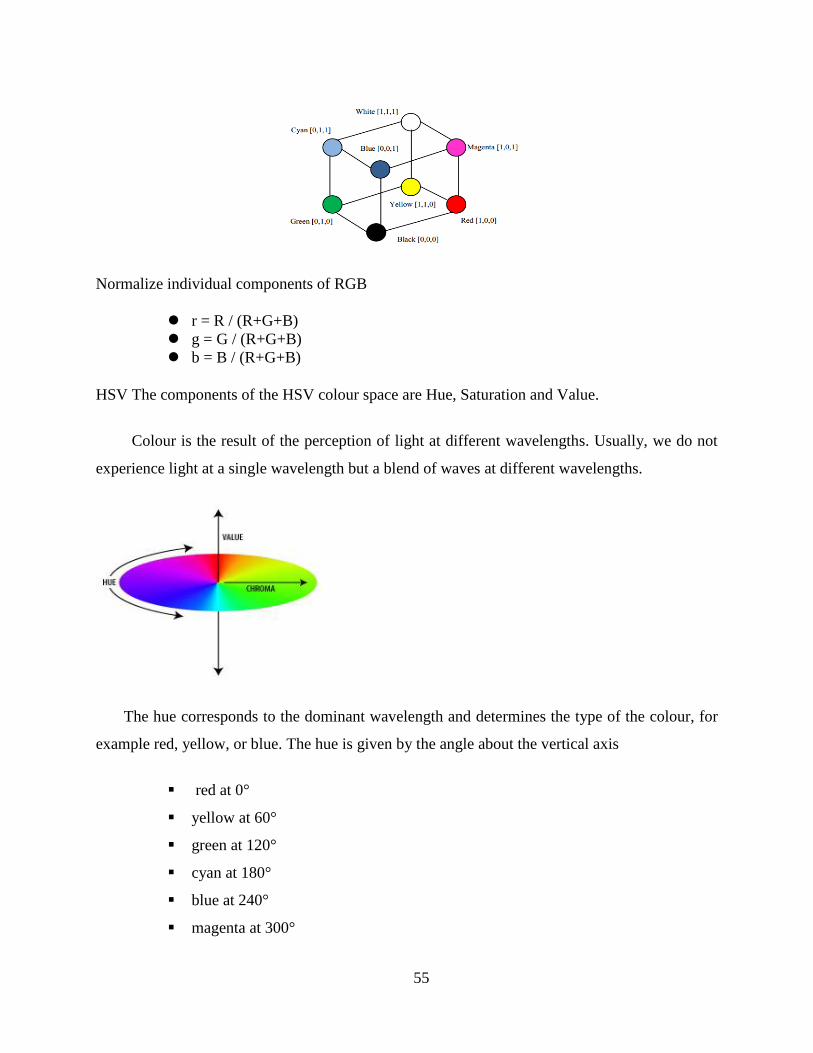
55
Normalize individual components of RGB
r = R / (R+G+B)
g = G / (R+G+B)
b = B / (R+G+B)
HSV The components of the HSV colour space are Hue, Saturation and Value.
Colour is the result of the perception of light at different wavelengths. Usually, we do not
experience light at a single wavelength but a blend of waves at different wavelengths.
The hue corresponds to the dominant wavelength and determines the type of the colour, for
example red, yellow, or blue. The hue is given by the angle about the vertical axis
red at 0°
yellow at 60°
green at 120°
cyan at 180°
blue at 240°
magenta at 300°

56
The saturation determines the purity of the colour. High saturation gives pure colours (narrow
wavelength band), while low saturation means colours mixed with a lot of white (white light
combines all the visible wavelengths).
The value determines the brightness. A value equal to zero represents absence of light, while
a high value gives bright colours.
The HSV spectrum of bright pure colours ( s = 1, v = 1 ). Notice the cyclicality of the hue. The
red corresponds both to h=0 and h=1.
h = 0 h = 1
Saturation, bright colours (v=1) with decreasing values of saturation.
S=1 S= 0.75 S= 0.5 S= 0.25
Value, Pure colours (s=1) with decreasing values of “value” (brightness).
V = 1 V = 0.75 V = 0.5 V = 0.25