Information Processing and Energy Dissipation in Neurons

Information Processing and Energy

Dissipation in Neurons

Lane McIntosh

Mathematics

University of Hawai’i at Manoa

Submitted in Partial Fulfillment of the Requirements for the Degree of

Master of Arts

April 2012

Thesis Committee

Susanne Still George WilkensDepartment of Information Department of Mathematicsand Computer Science

Abstract

We investigate the relationship between thermodynamic and information

theoretic inefficiency in an individual neuron model, the adaptive exponen-

tial integrate-and-fire neuron. Recent work has revealed that minimization

of energy dissipation is tightly related to optimal information processing, in

the sense that a system has to compute a maximally predictive model. In

this thesis we justify the extension of these results to the neuron and quan-

tify the neuron’s thermodynamic and information processing inefficiency as

a function of spike frequency adaptation.

Contents

List of Figures iv

1 Introduction 1

1.1 Physical Systems and their Computations . . . . . . . . . . . . . . . . . 1

1.2 Plan of Action . . . . . . . . . . . . . . . . . . . . . . . . . . . . . . . . 3

2 Background 4

2.1 Biology and the Neuron . . . . . . . . . . . . . . . . . . . . . . . . . . . 4

2.2 Probability Theory . . . . . . . . . . . . . . . . . . . . . . . . . . . . . . 12

2.3 Information Theory . . . . . . . . . . . . . . . . . . . . . . . . . . . . . 13

2.4 Far-from-Equilibrium Thermodynamics . . . . . . . . . . . . . . . . . . 19

2.5 Bridging Information Theory and Statistical Mechanics . . . . . . . . . 26

2.6 Thermodynamics of Prediction . . . . . . . . . . . . . . . . . . . . . . . 31

3 Methods 39

3.1 Model Description . . . . . . . . . . . . . . . . . . . . . . . . . . . . . . 39

3.2 Choice of Protocol x(t) . . . . . . . . . . . . . . . . . . . . . . . . . . . . 41

3.3 Choice of State s(t) . . . . . . . . . . . . . . . . . . . . . . . . . . . . . . 46

3.4 What is a Neuron in Equilibrium? . . . . . . . . . . . . . . . . . . . . . 47

4 Results 49

4.1 Adaptation Maximizes Memory and Predictive Power . . . . . . . . . . 50

4.2 Neurons Are Energy Efficient Across All Adaptation Regimes . . . . . . 50

5 Discussion 53

References 54

iii

List of Figures

3.1 Voltage responses of the adaptive exponential integrate-and-fire neuron

(bottom) to 1 second of injected current by the stimulus above it. Steady-

state mean current is 555 pA in all three stimuli. . . . . . . . . . . . . . 43

3.2 Voltage V and adaptation variable w of the adapting (a = 8) exponential

integrate-and-fire neuron to 1 second of stimulation by a step current. . 45

4.1 Total Memory, Predictive Power, and Nonpredictive information as a

function of adaptation. Here we quantify the sum of instantaneous mem-

ory, predictive power, and nonpredictive information of the adaptive ex-

ponential integrate-and-fire neuron model being driven out of equilibrium

by one second of the Ornstein-Uhlenbeck stimulus. Insets are example

voltage traces for a neuron with (from left to right) a = 0, 6, and 20

responding to a simple step of current. . . . . . . . . . . . . . . . . . . . 51

4.2 Instantaneous memory (blue), predictive power (green), nonpredictive

information (red), and the total information available in the stimulus

(grey). Bottom plots are spike rasters. The leftmost panes capture

the high spiking behavior of a non-adapting neuron, the middle panes

correspond to an adapting neuron (a = 6), and the rightmost panes

correspond to a non-spiking neuron. In low noise conditions, the analog

neuron captures the most information about the stimulus yet is the most

inefficient. . . . . . . . . . . . . . . . . . . . . . . . . . . . . . . . . . . . 52

iv

Acknowledgements

This project was first conceived by my advisor Susanne Still and Giacomo

Indiveri at ETH Zurich; I am especially indebted to Professor Still for help-

ing me at all stages of this research. I am also thankful to George Wilkens

for all the hours we spent pouring over stochastic differential equations,

and his patience with questions that always seem trivial in retrospect. I

also thank Robert Shaw, Jon Brown, John Marriott, and Eric Reckwerdt

for their conversations and advice relating to this thesis, and Paul Nguyen

for his explanation of “that ∪ symbol” on the first day of graduate real

analysis and his priceless companionship.

I am also grateful to the National Science Foundation and the Mathemat-

ics Department at the University of Hawaii, Manoa for their full financial

support that covered my entire time here.

1

Introduction

1.1 Physical Systems and their Computations

It might be counterintuitive to think that arbitrary physical systems perform compu-

tations and build models, but in many ways they do (1, 2, 3, 4). Since physical systems

change in response to forces from the external environment, we can consider the state

of the physical system at any given time as an implicit model of what has happened

previously.

Some of these implicit models are better than others. On a macroscopic scale, we

could say that a wind sock that provides a good indication of the strength and direc-

tion of wind provides a much better implicit model of its external environment than a

concrete wall. Similarly, the molecules in a strand of one’s DNA provide a better model

of our past than the same number of glucose molecules elsewhere. If we are to bring

this mindset to bear on the field of neuroscience, we might suppose that neurons are

very good at modeling, since they are able to communicate a finely detailed represen-

tation of our world solely through the generation of electrical action potentials (5). In

particular, we might suppose that aspects of neuron spiking, like spike adaptation, have

evolved in order to improve neurons’ ability to make these implicit models of their input.

Broadly speaking, neuroscience seeks to understand how thought and behavior emerge

from one particular physical system, the brain. Our brains have an incredible capacity

for gathering sensory information and constructing behaviorally-relevant representa-

1

1. INTRODUCTION

tions of the world via complex internal states. What exactly then are the structures

of the brain whose states process information, and even more importantly, within this

system, what are the physics of information processing?

In this thesis, we take the neuron to be the fundamental unit of information processing

in the brain, and apply a new theoretical result that the inefficiency of a system’s ability

to process information is exactly equivalent to the system’s energetic inefficiency (4).

One interpretation of this is that every system employs predictive inference insofar as

it operates efficiently (4).

This result bears a powerful implication for neuroscience - that a neuron’s ability to

represent information efficiently dictates how economically it consumes energy, and

vice-versa. Since a significant fraction of energy consumption in the neuron orches-

trates the propagation of action potentials (6), we expect that characteristic signatures

in neuron spike trains like spike frequency adaptation might arise from the minimiza-

tion of information processing inefficiency, or equivalently, the minimization of energy

dissipation.

While the theoretical relationship that energy dissipation is equivalent to the ineffec-

tiveness of a system’s implicit model has been proven true, its extension to the neuron

requires care. For one, the equality only holds for Markov systems with well defined

thermodynamic equilibria (4). Towards this end, we must determine what the “state”

of the neuron is exactly. Another consideration is that, although neurons are certainly

energetically efficient, neurons are known to perform discrimination (7) and incidence

timing (8) tasks that might differ significantly from predictive inference - perhaps per-

forming these tasks well is more important to the organism than a strict minimization

of energetic inefficiency. An additional challenge is the bewildering diversity of neurons

and the differing types of synaptic currents they are subjected to, which differ accord-

ing to the function of the neuron in its particular neural circuit (9).

In the following pages we will investigate whether or not neurons use one particular

mechanism, spike frequency adaptation, in order to accomplish this task of creating a

2

1.2 Plan of Action

good implicit model of their input by minimizing energetic and information processing

inefficiency.

1.2 Plan of Action

This thesis brings together research on statistical mechanics, information theory, neu-

roscience, and neuromorphic engineering, and our background chapter will be appro-

priately broad. We will first discuss neurons and how they are typically dealt with

mathematically, before we talk briefly about the conventions we adopt in our treatment

of probability distributions. We will then introduce relevant concepts and theorems in

information theory and a subset of results from statistical mechanics and far-from-

equilibrium thermodynamics, which we will be using later. We then discuss historical

results that have made connections between information theory and statistical mechan-

ics. This will set the stage for an in-depth discussion of the theoretical results from (4),

which form a basis for this thesis. Each section in the background chapter solely con-

tains past findings from other authors, even though at times we may take the stylistic

liberty of discussing a result as if we were deriving it for the first time.

Next we will cover our methods, starting with a description of the neuron model we

use in the paper, its relevance to actual neurons, the parameters typically used in the

neuroscience literature, how the model was derived, and how we simulate it. It is here

where we also make formal decisions as to the neuron’s state and the protocol that

drives it away from equilibrium. We also discuss in this chapter our methods for nu-

merically solving the system using the Runge-Kutta method.

Lastly, we present our findings and discuss future experimental work.

3

2

Background

2.1 Biology and the Neuron

Neurons are excitable cells found in the brain and elsewhere in the nervous system

from the mechanoreceptors in the bottoms of your feet to the interneurons of your

brain’s cortex, and have the extraordinary ability to capture and transmit information

via stereotyped electrical impulses called action potentials or spikes (9). While there

is significant variation from neuron to neuron in spike timing, action potential shape,

distribution of ion channel types that generate the spikes, and neurotransmitters that

modulate and relay information between neurons, all of the information a neuron re-

ceives and distributes can be represented mostly through it’s digitized spike time series

(10).

Before we can discuss how neurons are typically dealt with mathematically, we must

briefly familiarize ourselves with the biology of the neuron. Unlike canonical physical

systems like a harmonic oscillator or an ideal gas compressed by a piston, a biological

neuron has no a priori state, and we must use qualitative biological knowledge to make

a reasonable guess of what a neuron’s “state” would be. Of course, while the com-

plexity of a real neuron is not determined solely by the voltage across the neuron’s cell

membrane, perhaps from an information theoretic perspective it is not unreasonable

to simplify the entire physical state of a neuron down to the instantaneous voltage dif-

ference across its membrane, since the information transmitted by neurons is primarily

encoded in these voltage differences. This intuition about the simplified state of the

4


neuron will also be integral to our choice of neuron model.

Furthermore, it is important for the biology of the neuron to constrain our neuron

model, since otherwise we would have no idea as to whether or not our conclusions

are a good approximation for what we would find in vivo. Before delving into a brief

overview of how neurons are typically modeled both in theory and in silica, we also

briefly review the concept of spike frequency adaptation, and how adaptation might be

relevant to our application of (4) to the model neuron.

2.1.1 The Brain

In an average 3 pound adult human brain, there are approximately 1011 neurons, each

with roughly 7,000 connections to other neurons (11, 12). In comparison to other

sciences, knowledge about the brain has been painstakingly slow; although the brain

has been regarded as the seat of mental activity since the second century, it was not

even understood that the brain was comprised of cells until the nineteenth century (13).

One particularly elusive piece of this puzzle had been identifying which parts of the

brain give rise to mental activity, and how these structures integrate and process sen-

sory information, perform inferences, generate cohesive thoughts, and lead to behavior.

To this day, there is still considerable controversy over what the fundamental unit of

computation is in the brain (14, 15). Neurons interact with other neurons through ex-

citatory and inhibitory synapses, which can significantly sculpt information as it passes

from one neuron to another (16). The vast majority of neurons receive input from

many neighboring neurons, but ambiguity surrounds exactly where the integration of

all this information takes place. Oftentimes the connections between neurons form a

functional group that acts in synchrony; these groups, or circuits, are another candidate

for the fundamental unit of computation in the brain (14). Circuits in turn interact

with other circuits to form large networks of neurons, which have also been argued to

carry information not present at the individual neuron or circuit levels (17).

Historically progress in neuroscience has been driven by the development of new tech-

nologies used to sample and image activity in the brain, and to this day most of these

technologies have the capacity to only look at brain activity on small, disjoint subsets of

5

2. BACKGROUND

spatial and temporal resolution, resulting in neuroscience communities that have very

different views on the level of computation in the brain (18).

In this thesis, we make the reasonable assumption that significant information is con-

veyed by action potentials, even at the single neuron level. However, we are still not free

from controversy, since there is also disagreement as to how action potentials encode

information; specifically, there is disagreement over whether these action potentials en-

code information via the firing rate of the action potentials or via a precise temporal

code whereby the time between each action potential (called inter-spike intervals, or

ISIs) is important (19, 20, 21, 22, 23). Of course, choosing a single side is unnecessary,

and there is evidence of neurons that use both strategies; for instance, photoreceptors

in the retina are thought to be incidence detectors, and so temporal timing is of critical

importance, while in area V1 of visual cortex there are neurons known to encode the

orientation of edges in the visual field via spike rate (5).

Action Potentials

Neurons, like all other cells throughout the body, are made distinct from the extra-

cellular space by a lipid bilayer membrane that is impermeable to ions (9). However,

embedded in this membrane is the basis for all electrical signaling throughout the an-

imal kingdom - ion channels. Ion channels are macromolecular pores that selectively

transport ions back and forth through the cell membrane either passively (such that

ions flow through the pore along the ion’s concentration gradient) or actively (such that

energy in the form of adenosine triphosphate, ATP, is expended to move ions against

their concentration gradient), and are responsible for the production and transduction

of most signals generated by and sent to the brain - from the contraction of muscles to

the detection of sound waves (24).

Action potentials, the substrate for theories of coding and computation in neurons,

are rapid depolarizations of the cell membrane typically lasting < 1 ms generated by

Na+, K+, and Cl− ion channels (24).1 The potential difference (or voltage) of the neu-

ron’s intracellular environment with respect to the extracellular space is given by the

1Note that in action potentials outside of the human brain, for instance in cardiac action potentials,

Ca2+ ion channels are also involved, creating action potentials that are on the order of 100 times slower.

6


Goldman-Hodgkin-Katz equation as a function of the relative concentrations of these

ions inside and outside the cell,

Vneuron =RT

Fln

[PK+ [K+]out + PNa+ [Na+]out + PCl− [Cl−]inPK+ [K+]in + PNa+ [Na+]in + PCl− [Cl−]out

], (2.1)

where [ion] is the concentration of the ion, Pion is the permeability of the ion across the

cell membrane, R is the ideal gas constant, T is the temperature, and F is Faraday’s

constant (13). Note that a positive Vneuron then indicates that there are more positive

ions outside of the cell than inside. At rest, a typical value of Vneuron would be around

−70 mV, and in fact all excitable cells have a negative resting potential since there are

Na+-K+ channels that actively pump positive sodium ions into the extracellular space

and potassium ions into the cell (with 3 sodium ions leaving for every 2 potassium

ions entering) (24). At rest, the cell membrane is much more permeable to potassium

ions than sodium or chloride ions (i.e., there are far more open potassium channels

than open Na+ or Cl− channels), and so PNa+ >> max{PNa+ , PCl−} and the ratio

[K+]out/[K+]in dominates Vneuron (24). Since the sodium/potassium pump actively

drives up the concentration of potassium inside the cell, [K+]out/[K+]in < 1 resulting

in a negative Vneuron.

An action potential occurs when inward synaptic currents depolarize the membrane

potential and a large number of voltage-gated Na+ ion channels open, letting positive

sodium ions flow along their concentration gradient into the cell rapidly (9). Since this

further increases the membrane potential, even more voltage-gated sodium channels

are opened; in this manner, an action potential is an all-or-nothing response. At the

peak of the action potential, the sodium channels close and potassium channels open,

letting the voltage fall back to resting potential (9). After this occurs, there is a short

“refractory” period during which the membrane must be recharged by the active ion

channels, pumping Na+ ions back into the extracellular space and K+ ions back into

the cell (24).

Energy Consumption and Efficiency

With all of this shuttling of ions across the cell membranes of neurons, how substantial

is the energy cost of transmitting information along a neuron? Although the human

brain comprises only about 2% of our body mass, at rest the brain accounts for about

7

2. BACKGROUND

20% of oxygen consumption in the body and about 20% of the entire body’s metabolism

(6, 25). Most of this disproportional consumption of energy comes from the Na+-K+

pump, which must break a phosphate bond of ATP for every 3Na+/2K+ transported

across a neuron’s membrane (26). During a single action potential event, this translates

to 1.5× 108 ATP molecules that are used up by the Na+-K+ pump alone, with a total

energetic cost of almost 4.0×108 ATP (about 3.8×10−11 J) per action potential (26, 27).

Given the high energetic costs associated with information processing in neural tissue

and evidence that evolution strongly minimizes energy consumption while maintaining

the ability to adapt under changing environmental conditions (28), many theories of

energy efficient neural coding have been developed in the last four decades (29, 30, 31).

Most of these codes seek efficiency by maximizing representational capacity1 while re-

ducing the average firing rate, minimizing redundancy, or using sparse and distributed

codes (32, 33).

Beyond governing how information is encoded, the need for energy efficiency in neural

systems (without losing any signal to intrinsic noise) extends from the degree of inter-

neuron wiring miniaturization in the brain (34, 35) to the distribution of ion channels

in the cell membrane (36, 37), and has been seen as the unifying principle of neural

biophysics (37).

Spike-frequency Adaptation

One mechanism by which neurons are thought to reduce their firing rate and operate

more efficiently is spike-frequency adaptation (38). Spike-frequency adaptation is the

slow decrease in a neuron’s firing rate after it is exposed to a steady stimulus current,

and has been found in the neurons of a wide variety of organisms, from crustaceans to

humans (39). Adaptation in general is found in neurons and neural circuits on many

different timescales for the purpose of increased dynamic range and sensitivity to small

changes, and - at the loss of context - adaptation represents a maximization of the

information the neuron, or circuit, transmits about its sensory inputs, increasing the

1Treating the action potential as a binary event, the representational capacity in bits per unit time

of n neurons is C(n, np) = log2

[n!

(np)!(n−np)!

], where p ∈ [0, 1] such that np ∈ Z+ is the number of

neurons active (30).

8


efficiency of the neural code (40, 41).

Spike-frequency adaptation in particular is a ubiquitous feature of spiking neurons that

can be caused by a variety of mechanisms (42). After an action potential occurs, there is

a deep hyperpolarization (called an afterhyperpolarization, or AHP) during the action

potential’s refractory period; during repetitive spiking, these AHPs can accumulate,

slowing down the firing rate (24). In addition to these AHP currents, it is understood

that currents generated by voltage-gated, high-threshold K+ channels and the fast

sodium current can also give rise to spike-frequency adaptation (42, 43). Despite de-

tailed biophysical knowledge of mechanisms underlying spike-frequency adaptation, the

functional role of spike-frequency adaptation in computation is still relatively unclear

(39).

Neuron Models

Neuron models seek to describe the electrical activity of the cell via a system of differen-

tial equations, and generally fall into one of two general categories - simple, mathemat-

ically tractable models of neuron spiking behavior and biophysically detailed models

that simulate mechanisms underlying the neuron’s activity (44).

The history of theoretical models for neurons began with Louis Lapicque in 1907 with

one of the simplest model neurons, the integrate-and-fire neuron,

I(t) = CdV

dt, (2.2)

where I(t) is the current, C is the membrane capacitance, and V is the potential dif-

ference across the membrane (45). As current is injected, V increases until it reaches a

threshold Vthreshold, at which point V is reset to some resting potential and an action

potential is considered to have occurred.

The membrane of the cell has capacitance C due to the accumulation of positive and

negative charges on either side of the thin lipid bilayer membrane of the cell; this leads

to an electrical force that pulls oppositely-charged ions toward the other side, which

can be described as a capacitance C (13). In vivo, the movement of these ions across

9

2. BACKGROUND

the membrane with associated charge Q creates a current according to

I(t) =dQ

dt. (2.3)

The cell membrane however is only semipermeable, and so has a membrane resistance

R associated with it as ions are transported across the membrane. The ease at which

the current crosses the membrane, or conductance g, is accordingly the inverse of this

resistance, g = 1/R (24).

In contrast to simple models like 2.2, detailed biophysical models take account of these

conductances and ionic sources of current. In the earliest detailed biophysical model -

the Hodgkin and Huxley model - the current I(t) is broken up into component parts

I(t) = IC(t) +∑k

Ik(t), (2.4)

where IC(t) is the portion of injected current that contributes to building up a potential

difference across the membrane and the Ik are currents that pass through the sodium,

potassium, and unspecified leak ion channels (46). Each of these ion channels is associ-

ated with a conductance gk, a resting potential Ek given by 2.1 with all permeabilities

Pj = 0 for j 6= k, and gating variables m,n and h that determine the probability that a

channel is open (46). Looking back at our formulation for the integrate-and-fire neuron

in 2.2, we let IC(t) = C dVdt . Then substituting our new expression for IC(t) into 2.4

and expanding the ion channel currents with the parameters described above, we find

that the full Hodgkin and Huxley model is

CdV

dt= I(t)−

[gNam

3h(V − ENa) + gKn4(V − EK) + gL(V − EL)

](2.5)

=dm

dt= αm(V )(1−m)− βm(V )m (2.6)

=dn

dt= αn(V )(1− n)− βn(V )n (2.7)

=dh

dt= αh(V )(1− h)− βh(V )h, (2.8)

where each αi, βi are empirical exponential functions of voltage (47). Since the 1952

publication date of the Hodgkin-Huxley model, numerous additional models have been

proposed that make compromises between these disparate categories of simple func-

tional models and detailed biophysical ones (for a good overview see (46) or (48)).

10


Of particular interest to us will be the adaptive exponential integrate-and-fire neuron

(see Chapter 3), an elaboration of the integrate-and-fire neuron 2.2 that demonstrates

spike-frequency adaptation (49).

In Silico Models

Although electronic and neural circuits differ in countless ways including composition,

speed of electrical transmission, power usage, energy dissipation, representation of sig-

nals, memory storage, and plasticity, both involve the transmission of electrical signals

(50). And while replicating the nervous system in silico has failed up to the present

due primarily to the greater connectivity in neural systems relative to computers as

well as a deficient knowledge of the brain’s organizing principles (50), single neurons

have been successfully implemented as electronic circuits.

Single neurons are amenable to in silico modeling because many components of neu-

rons have analogous circuit components: the cell membrane is essentially a capacitor,

the ion channels imbedded in the membrane act as resistors, and the difference in ion

concentration inside and out of the cell that give rise to the membrane potential is a

battery that charges the capacitor. Neuromorphic engineering seeks to design either

analog or digital computer chips that emulate the behavior of real neurons, and to do

this, engineers must consider the density of electrical components, the complexity and

size of the circuit, the balance between analog and digital elements, and the energy

efficiency and consumption of the circuit (51).

Traditional computer implementations of neurons dissipate non-negligible amounts of

energy and consume roughly 8 orders of magnitude more energy per instruction1 than

biological neurons (52, 53). In 1990, it was correctly estimated that computers use 107

times as much energy per instruction than the brain does (54). This vast inefficiency

led to the development of analog, low(er)-power silicon implementations of neurons,

which still dissipate large amounts of power compared to the brain (51). In addition to

the drawback of needing to supply more power, implementations that dissipate large

1Here we consider an action potential to be an instruction in a biological neuron, albeit this is

somewhat unfair given that biological neurons could be considered to convey signals via firing rate,

which would require several action potentials.

11

2. BACKGROUND

amounts of energy limit the density and miniaturization of its component parts on ac-

count of thermal noise (51). In addition, neuromorphic prostheses intended to restore

movement, hearing, or vision to patients face serious clinical challenges due to brain

tissue damage caused by the dissipation of heat (55).1

To overcome these issues, Giacomo Indiveri and colleagues have recently developed

in silico implementations of the adaptive exponential integrate-and-fire neuron that

dramatically reduce the amount of dissipated energy, and so it will be possible in the

future to experimentally verify the theoretical predictions of this thesis (52).

2.2 Probability Theory

In this thesis we will assume knowledge of basic probability theory, but we will mention

a few key theorems and conventions that we will use later.

2.2.1 Normal Distribution

We say that a random variable X ∼ N(µ, σ2) when X is normally distributed with

mean µ and variance σ2, such that

p(x) =1

σ√

2πe−

(x−µ)2

2σ2 , (2.9)

where p(x) is the probability density function and the x are possible values of X.

2.2.2 First Moment

Let X be a random variable. We denote the average of X over a probability distribution

p by the angle brackets 〈X〉p. When the probability distribution is clear from the

context, we will occasionally reference the average as 〈X〉.2

1In order to avoid damaging brain tissue, a 6 × 6 mm2 array must dissipate less than 10mW of

energy (55, 56). As a comparison, a typical 7.88 mm × 7.53 mm Utah 100 microelectrode array used

today dissipates roughly 13 mW of energy (56).2Later this will especially occur when we average over the joint probability distribution of the

process’ state space s(t) and the space of protocols x(t).

12

2.3 Information Theory

2.2.3 Jensen’s Inequality

Theorem (Jensen’s Inequality) 2.2.1. Assume that the function g is measurable

and convex downward. Let the random variable X be such that 〈|X|〉 <∞. Then

g(〈X〉) ≤ 〈g(X)〉. (2.10)


Information as a mathematical quantity was first developed by Claude Shannon in his

seminal work, “A Mathematical Theory of Communication,” first published in 1948 (in

fact, upon realizing the generality of the theory, later publications changed the article

“a” to “the”) (57, 58). Shannon represents an arbitrary (discrete) information source

as a Markov process and then asks whether we can define a quantity that measures

how much information the process produces, and at what rate. We think of information

in this context as how interesting it is to discover the realization of the process. For

instance, if a process x(t) = 1 with probability Pr(x = 1) = 1 for all time t, then there

is no information in discovering what x actually is at any time t.

2.3.1 Entropy

Suppose we have a discrete random variable that can take one of n states with proba-

bilities p1, p2, ..., pn. Then a measure of information H should satisfy

1. H should be continuous in the pi.

2. If all the pi are equal, pi = 1n , then H should be a monotonic increasing function

of n. With equally likely events there is more choice, or uncertainty, when there

are more possible events.

3. If a choice is broken down into two successive choices, the original H should be

the weighted sum of the individual values of H.

This leads us to the important finding that

Theorem 2.3.1. The only H satisfying the above three assumptions is of the form

H = −Kn∑i=1

pi log pi, (2.11)

where K is a positive constant.

13

2. BACKGROUND

Proof. Let H be a function of the probability distribution, H(p1, p2, ..., pn). From

condition (2) we have H(

1n ,

1n , ...,

1n

)= f(n), where f is a monotonic increasing function

of n. Applying condition (3), we can break down a choice from rm equally likely

possibilities into a series of m choices each from r equally likely possibilities, such that

f(rm) = mf(r). (2.12)

Similarly, we have f(tn) = nf(t). Furthermore, we can choose n arbitrarily large and

find an m to satisfy

rm ≤ tn < rm+1. (2.13)

Taking logarithms and dividing by n log r, we then have

m

n≤ log t

log r≤ m

n+

1

n=⇒

∣∣∣∣mn − log t

log r

∣∣∣∣ < ε, (2.14)

where ε is arbitrarily small. Furthermore, since f is monotonic, f(rm) ≤ f(tn) ≤f(rm+1) implies that mf(r) ≤ nf(t) ≤ (m + 1)f(r), and so by dividing by nf(r), we

havem

n≤ f(t)

f(r)≤ m

n+

1

n=⇒

∣∣∣∣mn − f(t)

f(r)

∣∣∣∣ < ε. (2.15)

Combining (2.14) with (2.15), we find that certainly∣∣∣∣ f(t)

f(r)− log t

log r

∣∣∣∣ ≤ 2ε. (2.16)

Since ε is arbitrarily small, we are forced to have f(t) = f(r)log r log t, where f(r)

log r > 0 to

satisfy the monotonicity of f(t) required by condition (2). Since r is arbitrary, we letf(r)log r = K, where K is some positive constant.

Suppose we have∑n

i=1 ni choices with equal probabilities pi = ni∑ni

, where ni ∈ Z.

Then we have information measure

f(∑

ni

)= K log

∑ni. (2.17)

Alternatively, we could break up the∑ni choices into a choice from just n possibilities,

with probabilities p1, ..., pn, and then, if the ith possibility was chosen, a choice from

ni with equal probabilities. This would then have information measure

H(p1, ..., pn) +K∑

pi log ni. (2.18)

However, by condition (3), both of these information measures must be equivalent,

K log∑

ni = H(p1, ..., pn) +K∑

pi log ni, (2.19)

14


and so using the properties of logarithms and the observation that∑pi = 1,

H = K[∑

pi log∑

ni −∑

pi log ni

](2.20)

= −K[∑

pi log

(ni∑ni

)]= −K

∑pi log pi. (2.21)

We call this measure of information H entropy, and use ln ≡ loge for convenience,

measuring H in nats. Although most information theorists use log2 and measure H in

bits, our use of the natural logarithm anticipates the connection between information

theory and thermodynamics that we will explore later.

Out of convenience we take K = 1 and define the entropy of a discrete random variable

X with probability distribution p(x) as

H(X) = −∑x∈X

p(x) ln p(x), (2.22)

where X is the set of all values of X. This definition can easily be extended to the case

of two random variables X and Y with joint entropy,

H(X,Y ) = −∑x∈X

∑y∈Y

p(x, y) ln p(x, y). (2.23)

Since the “surprise value” or uncertainty of a process may change when another process

becomes known, it is natural to also consider conditional entropy H(X|Y ),

H(X|Y ) := −∑x∈X

∑y∈Y

p(x, y) ln p(x|y) (2.24)

= −〈ln p(x|y)〉p(x,y). (2.25)

15

2. BACKGROUND

The conditional entropy H(X|Y ) can also be seen as the difference between the joint

entropy H(X,Y ) and the entropy of the given variable, H(Y ) (59), since

H(X,Y ) = −∑x∈X

∑y∈Y

p(x, y) ln p(x, y) (2.26)

= −∑x∈X

∑y∈Y

p(x, y) ln p(y)p(x|y) (2.27)

= −∑x∈X

∑y∈Y

p(x, y) ln p(x)−∑x∈X

∑y∈Y

p(x, y) ln p(x|y) (2.28)

= −∑x∈X

p(x) ln p(x)−∑x∈X

∑y∈Y

p(x, y) ln p(x|y) (2.29)

= H(X) +H(X|Y ). (2.30)

2.3.2 Mutual Information

Consider two random variables X and Y with probability mass functions p(x) and p(y),

respectively, and joint probability mass function p(x, y). Mutual information is then

defined as the difference between the entropy of X and the conditional entropy of X

given Y (59),

I(X;Y ) := H(X)−H(X|Y ). (2.31)

From 2.30 we then have

I(X;Y ) = H(X)−H(X|Y ) (2.32)

= H(X) +H(Y )−H(X,Y ) (2.33)

= H(Y )−H(Y |X) (2.34)

= I(Y ;X), (2.35)

so mutual information is symmetric.

If we then expand the entropies using their probability mass functions, we further

16


find that

I(X;Y ) = H(X)−H(X|Y ) (2.36)

= −∑x∈X

p(x) ln p(x) +∑x∈X

∑y∈Y

p(x, y) ln p(x|y) (2.37)

= −∑x∈X

∑y∈Y

p(x, y) ln p(x) +∑x∈X

∑y∈Y

p(x, y) ln p(x|y) (2.38)

=∑x∈X

∑y∈Y

p(x, y) [ln p(x|y)− ln p(x)] (2.39)

=∑x∈X

∑y∈Y

p(x, y) lnp(x|y)

p(x)(2.40)

=∑x∈X

∑y∈Y

p(x, y) lnp(x, y)

p(x)p(y), (2.41)

where the last line follows from the definition of conditional probability of x given y,

p(x|y) = p(x,y)p(y) . Using our bracket notation, mutual information is then

I(X;Y ) =

⟨ln

p(x, y)

p(x)p(y)

⟩p(x,y)

. (2.42)

If X and Y are independent then p(x, y) = p(x)p(y) and mutual information can be

interpreted as measuring what you can learn about X from Y , and vice-versa; if X and

Y are independent, then there is zero mutual information, and we can learn nothing

about X from Y .

We can now introduce a new concept called relative entropy, or Kullback-Leibler diver-

gence, which will allow us to rewrite mutual information as DKL[p(x, y) || p(x)p(y)].

2.3.3 Relative Entropy

Relative entropy measures the difference between two probability distributions p(x)

and q(x),

DKL[p(x) || q(x)] =

⟨lnp(x)

q(x)

⟩p(x)

(2.43)

=∑x

p(x) lnp(x)

q(x). (2.44)

17

2. BACKGROUND

Theorem (Information Inequality) 2.3.1. Let X be a random variable with proba-

bility mass functions p(x) and q(x), where {x} are the possible values of X (59). Then

DKL[p || q] ≥ 0. (2.45)

Proof. Let A = {x : p(x) > 0} be the support of p(x). Then

−DKL[p || q] = −∑x∈A

p(x) lnp(x)

q(x)(2.46)

=∑x∈A

p(x) lnq(x)

p(x). (2.47)

By Jensen’s inequality 2.2.3, we take the passage of the natural logarithm under the

summation such that

−DKL[p || q] ≤ ln∑x∈A

p(x)q(x)

p(x)(2.48)

= ln∑x∈A

q(x). (2.49)

Next, since A ⊆ X and the sum of any probability distribution over all of it’s values

must be 1, we must have

ln∑x∈A

q(x) ≤ ln∑x

q(x) = ln 1 = 0. (2.50)

But since −DKL[p || q] ≤ 0, we must have DKL[p || q] ≥ 0.

Corollary 2.3.1. Let X and Y be two random variables. Then

I(X;Y ) ≥ 0. (2.51)

Proof. By our definitions 2.42 and 2.43, we have

I(X;Y ) =

⟨ln

p(x, y)

p(x)p(y)

⟩p(x,y)

(2.52)

= DKL[p(x, y) || p(x)p(y)], (2.53)

which by 2.45 is nonnegative.

18

2.4 Far-from-Equilibrium Thermodynamics

2.3.4 Inequalities

In addition to 2.45 and 2.51, from (59, 60) we also have the following inequalities:

• H(X) +H(Y ) ≥ H(X,Y ),

• H(X,Y ) ≥ H(X),

• H(X) ≥ H(X|Y ),

• H(X) ≥ 0, and

• I(X;Y ) ≥ I(X;Z) if X → Y → Z,

where X → Y → Z if the conditional distribution of Z depends only on Y and Z is

conditionally independent of X (59).


In our paradigm, we consider a stochastic physical system with state vector s driven

from equilibrium by some process x over a discrete time scale t ∈ {0, 1, . . . , τ}. Since

the physical system is stochastic, its state s given the protocol x is described by

the probability distribution p(s|x), and we let the time evolution of the system be

given by a discrete-time Markov process starting at t = 0 with transition probabilities

p(st|st−1, xt). For a Markov process (61), the transition to state st depends only on the

preceding state st−1, such that

p(st|st−1, xt) = p(st|st−1, st−2, . . . , s0, xt). (2.54)

At each step of the process x, we perform work W on the system, which in turn ab-

sorbs heat. Additionally, we let the physical system be embedded in an environment

of temperature T ; usually this amounts to coupling the system to a heat bath of con-

stant temperature such that any heat gained by the system is immediately whisked

away. While classical thermodynamics studies the relationships between these quanti-

ties of work and various forms of energy (most prominently, thermal and free energy)

where p(s|x) is an equilibrium distribution determined solely by x, far-from-equilibrium

thermodynamics is the study of these relationships in systems driven from equilibrium

where p(s|x) explicitly depends on the dynamics and history of the system’s trajectory

19

2. BACKGROUND

through state space (62).

Most results in far-from-equilibrium thermodynamics begin at specific statements of

the second law of thermodynamics, which asserts that systems tend to equilibrium,

and various theorems from probability theory (63). Although the second law of ther-

modynamics was first stated by Sadi Carnot in 1824, modern thermodynamics starts

with Rudolf Clausius’ restatement of the second law in 1855 (64). Clausius demon-

strated that for a cyclic process, ∮δQ

T≤ 0, (2.55)

where δQ is the amount of heat absorbed by the system, T is the temperature of

the system, and the inequality is strict in the case where the process is irreversible.1

Furthermore, Clausius provided the first definition of entropy S; letting S be a state

function that satisfies dS = δQ/T , Clausius then used (2.55) to state that entropy

changes obey

∆S ≥∫δQ

T. (2.56)

In words, entropy then quantifies the degree to which the system’s heat loss is irre-

versible. Realizing the statistical nature of this tendency towards disorder or “mixedup-

ness,” as the system absorbs heat, Ludwig Boltzmann then reformulated entropy S in

terms of the probabilities pi that a system has states si,

S = −kB∑i

pi ln pi, (2.57)

where kB is the Boltzmann constant.

Departing from this historical narrative, let us formally introduce the concepts of work

W and free energy F . In the context of thermodynamics, work was first defined as the

mechanical equivalent of heat (δW ∝ δQ), which was then later refined to accommodate

potential energy E,

δW = δQ− δE, (2.58)

where intuitively we see that performing work on the system is equivalent to adding

heat into the system while accounting for the system’s change in potential energy. The

1Here we will follow convention and use δ when referring to small but finite changes in a quantity

while d will be saved for infinitesimal values of a quantity.

20


concept of free energy F naturally arises from the desire to quantify the energy in

a system that is available for performing work, and was first given by Hermann von

Helmholtz in 1882 as

F = E − TS, (2.59)

although looser conceptions of free energy date back to the idea of affinity in the thir-

teenth century, when chemists sought an explanation for the force that caused chemical

reactions (65). We can see here that if we were to fix the total energy of the system,

the amount of energy available to do work decreases as the temperature or the entropy

of the system increases.

Using these definitions of work and free energy (and the linearity of integration), we

can restate the second law of thermodynamics (2.56) as

∆S ≥∫δE − δW

T=⇒

∫δW ≥ ∆E − T∆S =⇒ W ≥ ∆F, (2.60)

that is, the work we perform on the system is never less than the change in free energy

between the equilibrium state we started with and the equilibrium state we ended with

(63).

One key caveat to (2.60) is that it applies only to macroscopic systems; when we

move to the microscopic realm we must interpret W ≥ ∆F statistically, such that

〈W 〉 ≥ ∆F, (2.61)

where we are averaging W over the distribution p(s|x) of system states given the pro-

tocol (63). In addition to these statistical considerations, we must also pay special

attention to how we define free energy in a system arbitrarily far from equilibrium.

But first, what does it mean to be in equilibrium?

2.4.1 Equilibrium

Thus far we have only given thought to the state of the system conditioned on the

protocol. But what is the distribution of states before any work has been done to the

system? If our system is sufficiently isolated such that there is no net change in the

energy, matter, phase, or chemical potential of the system during the time before the

21

2. BACKGROUND

protocol begins, then we say that the system is in thermodynamic equilibrium.

Based on combinatorial counting of possible energy states and an application of the

second law of thermodynamics, Gibbs, Boltzmann, and Maxwell formalized this notion

of equilibrium with the Boltzmann distribution of system states. Given an initial con-

dition x0 of our protocol, the physical system starts in equilibrium if the probability

distribution p(s0|x0) of the initial state s0 given x0 is Boltzmann distributed according

to

peq(s0|x0) = e−β[E(s0, x0)−F (x0)], β =1

kBT, (2.62)

where E(s0, x0) is the energy of state s0 and protocol x0, and the free energy F (x0)

denotes the energy in the system available for performing work at equilibrium (66). As

we will see later in section 2.5, this equilibrium distribution can also be derived from

an application of information theory.

2.4.2 Free Energy

Recall that at equilibrium we had free energy F = E − TS where E was the internal

energy E(s, x) of the system, T is temperature, and S is entropy. Since the amount of

energy available to perform work in a system far from equilibrium will depend on how

far the system states are from equilibrium, we will need an additional non-equilibrium

free energy term proportional to the difference between the two distributions peq(st|xt)and p(st|xt). This additional free energy term is given as

F addt [p(st|xt)] := kBT DKL[p(st|xt) || peq(st|xt)], (2.63)

which we can interpret as the difference at time t between the actual distribution of

system states p(st|xt) and the distribution of states if the system were at equilibrium

(67).

Following (68), we also introduce the overall non-equilibrium free energy Fneq, which

we will define as the difference between the average system energy E(s, x) and the

temperature-scaled entropy of the system,

Fneq[p(s|x)] = 〈E(s, x)〉p(s|x) − TS, (2.64)

22


where entropy S = −kB∑p(s|x) ln p(s|x). We demonstrate below that this in fact is

equal to the sum of the equilibrium and non-equilibrium free energies Ft and F addt ,

respectively (4).

Theorem 2.4.1. Let the non-equilibrium free energy

Fneq[p(s|x)] = 〈E(s, x)〉p(s|x) − TS. (2.65)

Then Fneq[p(s|x)] is the sum of the equilibrium free energy F (x) and the non-equilibrium

free energy contribution F addt [p(s|x)].

Proof. Applying the definition of expectation, the non-equilibrium free energy becomes

Fneq[p(s|x)] = 〈E(s, x)〉p(s|x) − TS (2.66)

=∑

p(s|x)E(s, x) + kBT 〈ln p(s|x)〉p(s|x). (2.67)

Consider the triviality 0 = F (x) − F (x); noting that∑

s p(s|x) = 1 and F (x) is not a

function of s, we equivalently have 0 = F (x) −∑F (x)p(s|x). Then by linearity 2.66

becomes

Fneq =∑

p(s|x)E(s, x) + F (x) + kBT 〈ln p(s|x)〉p(s|x) −∑

F (x)p(s|x) (2.68)

= F (x) + kBT 〈ln p(s|x)〉p(s|x) +∑

p(s|x) [E(s, x)− F (x)] (2.69)

= F (x) + kBT 〈ln p(s|x)〉p(s|x) − kBT∑

p(s|x)

[− 1

kBT[E(s, x)− F (x)]

](2.70)

= F (x) + kBT 〈ln p(s|x)〉p(s|x) − kBT∑

p(s|x) ln e− 1kBT

[E(s,x)−F (x)]. (2.71)

But peq(s|x) = e− 1kBT

[E(s,x)−F (x)], and so

Fneq = F (x) + kBT 〈ln p(s|x)〉p(s|x) − kBT∑

p(s|x) ln peq(s|x) (2.72)

= F (x) + kBT 〈ln p(s|x)〉p(s|x) − kBT 〈ln peq(s|x)〉p(s|x), (2.73)

which by the property of logarithms gives

Fneq = F (x) + kBT

⟨ln

p(s|x)

peq(s|x)

⟩p(s|x)

, (2.74)

where the right-most term is the relative entropyDKL[p(s|x)||peq(s|x)]. Since F addt [p(s|x)]

is exactly kBT DKL[p(s|x)||peq(s|x)], we must then have

Fneq[p(s|x)] = F (x) + F addt [p(s|x)]. (2.75)

23

2. BACKGROUND

2.4.3 Dissipation versus Excess Work

This total non-equilibrium free energy represents the amount of work that could be ex-

tracted from the system, and in the case where we are performing work on the system,

we have Fneq[p(sτ |xτ )] ≥ Fneq[p(s0|x0)]. The difference between these final and initial

non-equilibrium free energies is then the amount of work we could get back out of the

system after our protocol has completed.

We follow (4) and define the dissipation of the system as the total amount of work

we have irretrievably lost during our protocol,

Wdiss := W −∆Fneq, (2.76)

where ∆Fneq = Fneq[p(sτ |xτ )]− Fneq[p(s0|x0)].

If the protocol progressed infinitely slowly and the system remained in equilibrium

for all time 0 ≤ t ≤ τ , the work performed on the system would equal the change in

equilibrium free energy ∆F = F (xτ ) − F (x0). We then define excess work to be the

difference between the actual work we put into the system and the smaller amount of

work we could have performed had our protocol run infinitely slowly with the system

at equilibrium,

Wex := W −∆F. (2.77)

This excess work Wex equals the system’s dissipation Wdiss in the case where the pro-

tocol ends with the system in equilibrium.

If we look at the average dissipation 〈Wdiss〉PS|X ,1 we repeat from (4) that

〈Wdiss〉PS|X = 〈W 〉PS|X −∆F − F addτ [p(sτ |xτ )] (2.78)

= 〈Wex〉PS|X − F addτ [p(sτ |xτ )] (2.79)

≤ 〈Wex〉PS|X . (2.80)

Hence on average the excess work we put into the system will always equal or exceed

the system’s dissipation.

1Here we are taking the expectation over the distribution PS|X = p(s0, . . . , sτ |x0, . . . , xτ ) of possible

system states given a particular protocol trajectory. Because the system is Markov and since we start

at equilibrium, this distribution is equivalent to peq(s0|x0)∏τt=1 p(st|st−1, xt).

24


2.4.4 Detailed Balance

Detailed balance is essentially a statement of microscopic reversibility at equilibrium,

such that for any two states sa and sb,

peq(sa → sb) = peq(sb → sa). (2.81)

Let a system with equilibrium state s0 be driven through some path to state sτ under

the change of protocol from x0 to xτ . We follow (62) and define work

W =τ−1∑t=0

E(st, xt+1)− E(st, xt) (2.82)

and heat

Q =τ∑t=1

E(st, xt)− E(st−1, xt). (2.83)

Then W + Q = E(sτ , xτ ) − E(s0, x0) = ∆E. With this in mind, we will now apply

detailed balance to the probabilities of the forward and reverse paths through state

space, PF (~s|~x) and PR(~s|~x), respectively.

Since our system is Markov, we first observe that

PF (~s|~x)

PR(~s|~x)=peq(s0|x0)

peq(sτ |xτ )

∏t

p(st|st−1, xt)

p(st−1|st, xt). (2.84)

We can then apply the definitions of equilibrium (2.62) and ∆E to this ratio, yielding

PF (~s|~x)

PR(~s|~x)= eβ(∆E−∆F )

∏t

p(st|st−1, xt)

p(st−1|st, xt), (2.85)

where ∆F = F (xτ ) − F (x0) is the change in equilibrium free energy. If we assume

detailed balance, which would require that the protocol keep the system in equilibrium

during its entire duration, then

PF (~s|~x)

PR(~s|~x)= eβ(∆E−∆F )

∏t

peq(st|xt)peq(st−1|xt)

. (2.86)

Substituting the definition of the equilibrium distribution again, we obtain

PF (~s|~x)

PR(~s|~x)= eβ(∆E−∆F ) · e−β

∑t[E(st,xt)−E(st−1,xt)] (2.87)

= eβ(Q+W−∆F ) · e−βQ (2.88)

= eβ(W−∆F ) = eβWex , (2.89)

25

2. BACKGROUND

that is, the degree of reversibility of the path through state space is equal to eβWex .

This last equality is known as the Crooks equation.1

2.4.5 Jarzynski’s Work Relation

Using detailed balance, Crooks then proved the following work relation (66).

Theorem (Jarzynski’s Work Relation) 2.4.1. Let W be work, ∆F be the free

energy difference F (xτ )− F (x0), and β = 1kBT

.2 Then

〈e−βW 〉 = e−β∆F . (2.90)

Proof. The average 〈e−βW 〉 is taken over all possible paths through state space over all

protocols from x0 to xτ ; i.e., we are averaging over PF . Then by applying 2.89 we have

〈e−βW 〉PF = 〈e−βW PFPR〉PR (2.91)

= 〈e−βW eβWex〉PR (2.92)

= 〈e−β(W−Wex)〉PR . (2.93)

But Wex = W −∆F , and so 〈e−βW 〉PF = 〈e−β∆F 〉PR . Furthermore, β is just a constant

and ∆F only depends on equilibrium values F (xτ ) and F (x0), so the expectation

brackets vanish, leaving 〈e−β∆F 〉PR = e−β∆F . Hence 〈e−βW 〉 = e−β∆F .

This result nicely constrains the possible distributions of work values W even when

the system is driven far from equilibrium; the theorem also implies that we can measure

equilibrium free energy differences from the behavior of the system far from equilibrium

(63).

2.5 Bridging Information Theory and Statistical Mechan-

ics

Historically there have been several results relating information theory and statistical

mechanics, most notably by E.T. Jaynes in the 1950’s and Rolf Landauer in the 1960’s.

1The Crooks equation is a special case of Crooks’ Fluctuation Theorem, which states that PF (+ω)PR(−ω) =

e+ω, where ω is the entropy production of the driven system with microscopically reversible dynamics

over some time duration (62).2Note that T is not the temperature during the process, which could be far from equilibrium where

temperature is not defined. Rather, T is the temperature of the heat bath coupled to the system.

26

2.5 Bridging Information Theory and Statistical Mechanics

As we will see in the next section, these results are extended by the recent findings of

Still et al. 2012 (4).

2.5.1 E.T. Jaynes

In 1957, E.T. Jaynes published two landmark papers on the subject of information

theory and statistical mechanics. In these two papers, Jaynes reinterpreted statistical

mechanics as a form of statistical inference rather than a physical theory with as-

sumptions outside of the laws of mechanics (69, 70). Partially driven by the inability

of classical thermodynamics to generalize to non-equilibrium conditions, Jaynes’ ap-

proach removed the need for additional assumptions like ergodicity, metric transitivity,

and equal a priori probabilities.

Suppose we have a system with n discrete energy levels Ei(α1, α2, . . . ), where each

αj is an external parameter such as volume, gravitational potential, or position of op-

tical laser trap. Then if we only know the average energy 〈E〉 of the system, we cannot

solve for the probabilities pi such that

〈E(α1, α2, . . . )〉 =n∑i=1

piEi(α1, α2, . . . ) (2.94)

unless our knowledge is augmented by (n − 2) more conditions in addition to the

normalization requirementn∑i=1

pi = 1. (2.95)

This problem of choosing the probabilities is inherently a statistical one,1 and if we

are to consider probabilities as a reflection of our ignorance, then a good choice of

pi is that which correctly represents our state of knowledge while remaining maxi-

mally unbiased or uncertain with respect to what we do not know. Since entropy

H(p1, p2, . . . , pn) = −∑ pi ln pi is a unique, unambiguous criterion for this amount of

uncertainty (see 2.3.1), we can infer the probabilities pi by maximizing their entropy

subject to what is known.

1In fact, this is a very old statistical problem, dating back to Pierre-Simon Laplace’s “Principle of

Insufficient Reason” in the early 1800’s.

27

2. BACKGROUND

Subject to the constraints 2.94 and 2.95, we can then maximize entropy by introducing

the Lagrangian function Λ with multipliers λ and µ such that

Λ(pi, λ, µ) = −n∑i=1

pi ln pi − λ(

n∑i=1

pi − 1

)− µ

(n∑i=1

piEi − 〈E〉), (2.96)

where we dropped the dependence on α1, α2, . . . from the notation of Ei and 〈E〉 out

of convenience.

Setting ∇pi,λ,µΛ(pi, λ, µ) = 0, we then find that we must have

∂Λ

∂pi= −(ln pi + 1)− λ− µEi = 0. (2.97)

Letting λ1 = λ+ 1, 2.97 then gives us our choice of each pi as

pi = e−λ1−µEi . (2.98)

Substituting this choice into the constraints 2.94 and 2.95 we find that

λ1 = lnn∑i=1

e−µEi and 〈E〉 =

∑ni=1 e

−µEiEi∑ni=1 e

−µEi= − ∂

∂µln

n∑i=1

e−µEi . (2.99)

The quantity∑n

i=1 e−µEi is commonly known as the partition function Z(µ, α1, α2, . . . ).

Substituting in the value of λ1, the probability pi that the system is in energy state Ei

is then

pi = e−λ1−µEi(α1,α2,... ) =e−µEi(α1,α2,... )∑n

i=1 e−µEi

. (2.100)

It now becomes clear why Z(µ, α1, . . . ) =∑n

i=1 e−µEi is known as the partition func-

tion: by means of Z(µ, α1, . . . ), we can determine how to partition our probabilities∑ni=1 pi = 1 among the different system states. This realization is crucial, since the

entire motivation of statistical mechanics is a desire to move easily between the mi-

croscopic properties of a system (like the positions and momenta of particles that give

rise to the individual energy levels Ei) and the macroscopic properties of the system

(things like temperature T and all the other external parameters α1, α2, . . . ).

Empirically, we find that µ = 1/kBT , where kB is Boltzmann’s constant and T is

temperature; this is also commonly referred to as thermodynamic β in the statistical

28

2.5 Bridging Information Theory and Statistical Mechanics

mechanics literature (69). This empirical finding can now be used to calculate several

quantities that interest us, like thermodynamic entropy and free energy.

Proceeding with the usual definition 2.59 of free energy F (T, α1, α2, . . . ) = E − TS,

Jaynes proceeds to show that

F (T, α1, α2, . . . ) = kBT lnZ(T, α1, α2, . . . ). (2.101)

Furthermore, since −∂F∂T = − ∂

∂T [E − TS] = S, we have thermodynamic entropy

S = −kB∑

pi ln pi. (2.102)

In addition to being equal mathematically aside from the Boltzmann constant kB, the

thermodynamic and information entropy terms are conceptually identical from this

vantage point, since both are essentially statements of statistical inference.1

2.5.2 Landauer’s Principle

While E.T. Jaynes interpreted the results of statistical mechanics as byproducts of

maximum entropy inference rather than new physical laws, Rolf Landauer took a dif-

ferent approach and emphasized the physical nature of information. In 1961, Landauer

connected the erasure of one bit of information with an energy cost of at least kBT ln 2

per bit2 (71). Initially appearing in an article of the IBM journal, Landauer’s intent

was to identify the lower limit of energy consumption in computing machines. How-

ever, this finding was remarkable for suggesting that arbitrary physical systems carried

out computations by means of transitions between their states (72). Extending this

in subsequent papers, Landauer argued that information is always tied to a physical

representation - the electrical state of a paired transistor and capacitor in a computer’s

memory cell, a DNA configuration, the up or down spin of an electron, or the state of

a neuron - and is never purely abstract (1).

1Recall also that Shannon proved entropy H is a unique measure of uncertainty (given his re-

quirements) up to a multiplicative constant K and the choice of the logarithm’s base. In statistical

mechanics we simply take K = kB instead of K = 1 and use natural log instead of the logarithm base

two.2In the 1950’s von Neumann proposed that any logical operation costs at least T ln 2. However,

Landauer showed that when computation is done reversibly, no dissipation occurs, and in fact the only

theoretical energy cost of computation lies in the erasure of information.

29

2. BACKGROUND

Suppose we erase one bit of information,∑n

i=1 pi log2 pi = 1. We can use the change

of base formula logb x = lnxln b to convert 1 bit to nats according to ln 2Hbits = Hnats.

Scaling this by Boltzmann’s constant we get kB ln 2Hbits = S, where S is thermody-

namic entropy. Landauer proposed that the physical nature of information implied that

erasing information Hbits in a system must be compensated by an increase of entropy

S ≥ kB ln 2Hbits elsewhere to preserve the second law of thermodynamics.

In order to find the minimum energy expenditure for information erasure, suppose

that we put work into the system to perform this computation such that the free en-

ergy gained by the system is F ≥ 0. According to 2.59 we must then have E ≥ TS.

Since erasing 1 bit increases the thermodynamic entropy by kB ln 2, we have a neces-

sary energy expenditure of E ≥ kBT ln 2 in order to compensate for the increase in

energy. Landauer argued that the necessity of this energy expenditure follows from the

second law of thermodynamics (the entropy of a closed system is nondecreasing) and

the assumption that a closed system has a finite maximum entropy. To avoid reaching

this maximum, the system must eventually expend energy on the order of kBT ln 2 per

additional bit it wants to compute.

Still et al. 2012 (4) rephrase Landauer’s limit in the language of far-from-equilibrium

thermodynamics. Suppose that the information He is being erased by our protocol

xt for time 0 ≤ t ≤ τ . Then we could compute the total information erased as the

reduction in entropy He = H(s0|x0)−H(sτ |xτ ).1

From the above rationale, recall that we must expend energy to erase He. According

to equation 2.58 (a statement of the first law of thermodynamics) this energy change

is related to the heat added to the system and work done by the system,

∆E = Q−W. (2.103)

From Landauer’s insight that ∆E ≥ kBTHe, together with the definitions of total non-

equilibrium free energy (2.66) and dissipation (2.76), we can take the average of 2.103

1Now we will measure He in nats. This means that the energy cost of erasing He will simply be

E ≥ kBTHe.

30

2.6 Thermodynamics of Prediction

and see that

∆E = 〈Q−W 〉 (2.104)

kBTHe ≤ 〈Q−W 〉 (2.105)

= 〈Q〉 − 〈W 〉 (2.106)

= 〈Q〉 − (〈Wdiss〉+ ∆Fneq) (2.107)

= 〈Q〉 − (〈Wdiss〉+ 〈E(sτ , xτ )〉+ kBT 〈ln p(sτ |xτ )〉 (2.108)

− 〈E(s0, x0)〉 − kBT 〈ln p(s0|x0)〉). (2.109)

Recalling that He = H(s0|x0)−H(sτ |xτ ) = 〈ln p(s0|x0)〉 − 〈ln p(sτ |xτ )〉,

kBTHe ≤ 〈Q〉 − (〈Wdiss〉+ ∆E − kBTHe) (2.110)

kBTHe ≤ 〈Q〉 − 〈Wdiss〉 −∆E + kBTHe (2.111)

∆E + 〈Wdiss〉 ≤ 〈Q〉 (2.112)

kBTHe + 〈Wdiss〉 ≤ 〈Q〉, (2.113)

where He is the information erased measured in nats, Wdiss is the energy dissipation,

and Q is the energy absorbed by the system. In words, this says that the average

heat absorbed by the system during the erasure of information is lower bounded by the

minimum energy cost of the erasure plus the thermodynamic inefficiency of the erasure

protocol. This implies that the erasure protocol must minimize its average dissipated

energy 〈Wdiss〉 to approach Landauer’s limit.


Keeping the conventions used in 2.4 we now review the results of Still et al. 2012, which

draw explicit relationships between thermodynamic dissipation Wdiss and information

theoretic inefficiency (4).

Consider a physical system in thermodynamic equilibrium that is driven through its

state space by a protocol xt ∈ {x0, . . . , xτ} governed by some probability distribution

PX(x0, . . . xτ ). Let us denote the system’s state at (discrete) time t as st; then at

any given time t the system state st ∈ {s0, . . . , sτ}. Suppose as in section 2.4 that

the dynamics of the system states st are described by the discrete Markov transition

31

2. BACKGROUND

probabilities p(st|st−1, xt) and that a change in the driving signal x0 → x1 forces the

system out of equilibrium from s0 → s1 according to p(s1|s0, x1).1 As before we also

couple the system to a heat bath at constant temperature T so that it can dissipate

any heat Q absorbed by the system.

As before, the equilibrium distribution is given by peq(s|xt) := e−β(E(s,xt)−F (xt)) and

the probability p(st|xt) of state st after the protocol has changed to xt is given by the

average of transitions from all possible st−1 to st, 〈p(st|st−1, xt)〉p(st−1|xt). We also note

that the probability of a specific path S through state space, conditional on a protocol

X = {x0, . . . xτ}, is

PS|X = peq(s0|x0)τ∏t=1

p(st|st−1, xt), (2.114)

and the joint probability of state and protocol paths S and X is

PS,X = p(x0)peq(s0|x0)

τ∏t=1

p(xt|x0, . . . , xt−1)p(st|st−1, xt). (2.115)

2.6.1 Instantaneous Inefficiency

We now define two information theoretic terms. Let the system’s instantaneous memory

be the mutual information between the system’s current state st and the protocol xt

at that time,

Imem(t) = I(st;xt) :=

⟨ln

[p(st, xt)

p(st)p(xt)

]⟩p(st,xt)

(2.116)

=

⟨ln

[p(st|xt)p(st)

]⟩p(st|xt)p(xt)

. (2.117)

Since the dynamics of st are determined by xt and st−1, presumably the system state

contains some information about the protocol. The degree to which the system can then

predict the next instantiation of the protocol is given by the instantaneous predictive

1It is worth noting that the conditional distribution p(st−1|xt) of st−1 immediately after xt−1 → xt

and the conditional distribution p(st|xt) describing the system after it adjusts to the signal change

xt−1 → xt are not the same in general, and neither is necessarily an equilibrium distribution.

32


power,

Ipred(t) = I(st;xt+1) :=

⟨ln

[p(st, xt+1)

p(st)p(xt+1)

]⟩p(st,xt+1)

(2.118)

=

⟨ln

[p(st|xt+1)

p(st)

]⟩p(st|xt+1)p(xt+1)

. (2.119)

The dynamics of the system states constitute an implicit model of the protocol, and

the instantaneous predictive power quantifies how effectively this implicit model can

predict the future trajectory of the protocol. Essentially, the predictive power then

represents how well the system’s knowledge about xt generalizes to xt+1.

If we then fix how well the system remembers xt, an implicit model of the protocol will

become increasingly ineffective as its predictive power decreases. A natural measure

of this information processing inefficiency is the systems’s instantaneous nonpredictive

information

Inonpred(t) = Imem(t)− Ipred(t). (2.120)

Recalling how we quantified non-equilibrium thermodynamic inefficiency as Wdiss in

2.76, we are now prepared to ask if there is a relationship between the system’s ther-

modynamic inefficiency and the system’s information theoretic inefficiency. In the same

vein as instantaneous memory and predictive power, we define an average “instanta-

neous” dissipation 〈Wdiss(xt → xt+1)〉 that quantifies only the energy dissipated during

the protocol transition from xt to xt+1,

〈Wdiss(xt → xt+1)〉 := 〈W (st;xt → xt+1)〉p(st,xt,xt+1) − 〈∆Fneq(xt → xt+1)〉p(xt,xt+1).

(2.121)

In words, the dissipated energy during our protocol step xt → xt+1 is equivalent to the

loss in energy we experience due to the work we put into the system, minus the gain

in energy due to our work increasing the free energy of the system. With this defined,

we can now introduce the first key result in the thermodynamics of prediction.

Theorem 2.6.1. Given the definitions and setup above, the instantaneous nonpredic-

tive information scaled by kBT is exactly the thermodynamic inefficiency of changing

the protocol from xt to xt+1, averaged over all possible paths through the state space of

the system and over all protocols,

kBT [I(st;xt)− I(st;xt+1)] = 〈Wdiss(xt → xt+1)〉. (2.122)

33

2. BACKGROUND

Proof. Recalling our formulation of mutual information in terms of conditional entropy

2.37, we have

I(st;xt)− I(st;xt+1) = H(st)−H(st|xt)− [H(st)−H(st|xt+1)] (2.123)

= H(st|xt+1)−H(st|xt). (2.124)

Next, we can use our definition of non-equilibrium free energy 2.64 to rewrite the

entropies above as thermodynamic quantities. Since non-equilibrium free energy

Fneq[p(s|x)] = 〈E(s, x)〉p(s|x) − TS (2.125)

= 〈E(s, x)〉p(s|x) + kBT∑

p(s|x) ln p(s|x) (2.126)

βFneq[p(s|x)] = β〈E(s, x)〉p(s|x) +∑

p(s|x) ln p(s|x), (2.127)

we can average over p(x) to obtain

β〈Fneq[p(s|x)]〉p(x) = β〈E(s, x)〉p(s|x)p(x) +∑∑

p(s|x)p(x) ln p(s|x) (2.128)

= β〈E(s, x)〉p(s,x) +∑∑

p(s, x) ln p(s|x) (2.129)

= β〈E(s, x)〉p(s,x) −H(s|x). (2.130)

Hence

H(st|xt+1) = β(〈E(st, xt+1)〉p(st,xt+1) − 〈Fneq[p(st|xt+1)]〉p(xt+1)

)(2.131)

and

H(st|xt) = β(〈E(st, xt)〉p(st,xt) − 〈Fneq[p(st|xt)]〉p(xt)

). (2.132)

We can then rewrite 2.123 in terms of these thermodynamic differences,

I(st;xt)− I(st;xt+1) = β(〈E(st, xt+1)〉p(st,xt+1) − 〈Fneq[p(st|xt+1)]〉p(xt+1)

)− β

(〈E(st, xt)〉p(st,xt) − 〈Fneq[p(st|xt)]〉p(xt)

), (2.133)

which, by rearranging the terms, becomes

I(st;xt)− I(st;xt+1) = β(〈E(st, xt+1)〉p(st,xt+1) − 〈E(st, xt)〉p(st,xt)

)− β

(〈Fneq[p(st|xt+1)]〉p(xt+1) − 〈Fneq[p(st|xt)]〉p(xt)

). (2.134)

Adopting our definition of work W from 2.82,

W =

τ−1∑t=0

E(st, xt+1)− E(st, xt), (2.135)

34


and using linearity of expectation, we can simplify 2.134 considerably:

I(st;xt)− I(st;xt+1) = β〈W (xt → xt+1)〉p(st,xt+1)

− β〈∆Fneq(xt → xt+1)〉p(xt+1,xt). (2.136)

Recall from 2.76 that Wdiss = W − ∆Fneq; then W (xt → xt+1) − ∆Fneq(xt → xt+1)

must be the dissipation that occurs only during the work step xt → xt+1. Taking the

average of the non-equilibrium free energy change over the distribution of states st and

using linearity of expectation again, this observation gives us

I(st;xt)− I(st;xt+1) = β〈W (xt → xt+1)−∆Fneq(xt → xt+1)〉p(xt+1,xt,st)(2.137)

= β〈Wdiss(xt → xt+1)〉, (2.138)

where β = 1/kBT .

The energy dissipated by the system as the protocol moves from xt → xt+1 is then

fundamentally equivalent to the amount of system memory that is not predictive of

xt+1.

2.6.2 Longterm Inefficiency

By summing over all time steps 0 ≤ t ≤ τ , we can then obtain a lower bound for the

total energy dissipated by the protocol,

β〈Wdiss〉 ≥ Imem − Ipred, (2.139)

where

Imem =

τ−1∑t=0

I(st;xt) and Ipred =

τ−1∑t=0

I(st;xt+1). (2.140)

Hence when we consider an arbitrarily long process, the thermodynamic efficiency of

the system is limited by its information processing inefficiencies.

Theorem 2.6.1. The energy dissipated over the entire protocol has the lower bound


where 〈Wdiss〉 is the total dissipation averaged over all protocols.

35

2. BACKGROUND

Proof. Recall the definition of 〈Wdiss(xt → xt+1)〉 from 2.121,

〈Wdiss(xt → xt+1)〉 := 〈W (st;xt → xt+1)〉p(st,xt,xt+1) − 〈∆Fneq(xt → xt+1)〉p(xt,xt+1).

(2.142)

Summing over the entire protocol and using the linearity of expectation gives us

τ−1∑t=0

〈Wdiss(xt → xt+1)〉 =

⟨τ−1∑t=0

W (xt → xt+1)

⟩p(s,x)

−⟨τ−1∑t=0

∆Fneq(xt → xt+1)

⟩p(x)

(2.143)

τ−1∑t=0

〈Wdiss(xt → xt+1)〉 = 〈W 〉p(s,x) −⟨τ−1∑t=0

∆Fneq(xt → xt+1)

⟩p(x)

. (2.144)

Noting then that

∆Fneq(xt → xt+1) = Fneq[p(st|xt+1)]− Fneq[p(st|xt)] (2.145)

and

∆Fneq(st → st+1) = Fneq[p(st+1|xt+1)]− Fneq[p(st|xt+1)], (2.146)

we rewriteτ−1∑t=0

∆Fneq(xt → xt+1) =

τ−1∑t=0

Fneq[p(st|xt+1)]−τ−1∑t=0

Fneq[p(st|xt)] (2.147)

=

τ−1∑t=0

Fneq[p(st|xt+1)]−τ∑t=1

Fneq[p(st|xt)] (2.148)

− Fneq[p(s0|x0)] + Fneq[p(sτ |xτ )](2.149)

= −τ−1∑t=0

∆Fneq(st → st+1)− Fneq(0) + Fneq(τ) (2.150)

= ∆Fneq −τ−1∑t=0

∆Fneq(st → st+1). (2.151)

Substituting this into 2.143,

τ−1∑t=0

〈Wdiss(xt → xt+1)〉 = 〈W 〉p(s,x) −⟨

∆Fneq −τ−1∑t=0

∆Fneq(st → st+1)

⟩p(xt,xt+1)

(2.152)

τ−1∑t=0

〈Wdiss(xt → xt+1)〉 = 〈W 〉p(s,x) −∆Fneq +

⟨τ−1∑t=0


⟩p(xt,xt+1)

,(2.153)

where each 〈Wdiss(xt → xt+1)〉 is averaged over all protocols p(xt, xt+1) as well. By

definition of Wdiss = W −∆Fneq in 2.77 the previous equality becomes

τ−1∑t=0

〈Wdiss(xt → xt+1)〉 = 〈Wdiss〉p(x) +

⟨τ−1∑t=0


⟩p(xt,xt+1)

. (2.154)

36


Define

〈∆F relaxneq 〉 :=

⟨τ−1∑t=0


⟩p(x)

. (2.155)

Since the system will relax towards equilibrium on average, the free energy of the sys-

tem at the end of a relaxation step st → st+1 will be lower than the system’s initial

free energy. This implies that the above quantity will always be less than or equal to

zero.

Now we can apply Theorem 2.6.1 and the linearity of expectation so that

τ−1∑t=0

〈Wdiss(xt → xt+1)〉 = 〈Wdiss〉p(x) +

⟨τ−1∑t=0


⟩p(x)

(2.156)

τ−1∑t=0

〈kBT (I[st;xt]− I[st;xt+1])〉 = 〈Wdiss〉p(x) + 〈∆F relaxneq 〉 (2.157)

kBT (Imem − Ipred) = 〈Wdiss〉p(x) + 〈∆F relaxneq 〉. (2.158)

Furthermore, since

〈∆F relaxneq 〉 ≤ 0, (2.159)

we must have


where β = 1/kBT .

Intuitively, we expect this inequality in place of the equality 2.6.1 because we are

not just summing over all of our work steps, but also summing over the periods between

when we advance our protocol xt → xt+1. In between these work steps the system will

relax towards equilibrium on average. The size of the difference between β〈Wdiss〉 and

Imem−Ipred is then proportional to how far we let our system relax towards equilibrium

between our work steps. The longer we let the system relax, the more dissipation we

allow.

Therefore the overall inability of a system to implicitly model its inputs, scaled by

kBT , gives the average minimum amount of energy that must be dissipated by a sys-

tem as it is driven from x0 to xτ .

37

2. BACKGROUND

2.6.3 Refining Landauer’s Limit

Interestingly, this can then be used to refine Landauer’s Principle 2.113 (4),

kBTHe + 〈Wdiss〉 ≤ 〈Q〉,

where He is the information erased during the protocol measured in nats, 〈Wdiss〉 is

the average energy dissipation over the course of the protocol, and 〈Q〉 is the average

energy absorbed by the system during the protocol.

Using the relation 2.156 that

β〈Wdiss〉 = Imem − Ipred + β〈∆F relaxneq 〉,

where β = 1/kBT , we must then have

〈Q〉 ≥ kBTHe + 〈Wdiss〉 (2.161)

= kBTHe + (kBTImem − kBTIpred + 〈∆F relaxneq 〉) (2.162)

= kBT (He + Imem − Ipred) + 〈∆F relaxneq 〉 (2.163)

≥ kBT (He + Imem − Ipred), (2.164)

where the last line follows from 〈∆F relaxneq 〉 ≥ 0 (equation 2.159). The heat cost of eras-

ing He nats of information is then lower bounded by the sum of the information erased

He and the amount of nonpredictive information Imem − Ipred, scaled by kBT .

This is really rather remarkable, since for systems where the intuition holds that

Imem − Ipred ≥ 0, this represents a tighter bound on the energy required for erasing

information. In particular, a system with fixed memory must be predictive in order to

approach Landauer’s limit (4). We shall investigate in the remaining chapters whether

a model neuron is such a system where, given fixed memory, nonpredictive information

is minimized to ensure thermodynamic efficiency.

38

3

Methods

3.1 Model Description

As we saw at the beginning of Chapter 2, neuron models range from detailed, biophysically-

realistic neuron models with many parameters to simple integrate-and-fire neurons that

are more mathematically tractable. In addition to choosing a model that conforms well

to biological data, the model must be simple enough for the kinds of analyses planned.

We chose to work with an adaptive exponential integrate-and-fire neuron, developed

by Romain Brette and Wolfram Gerstner in 2005 (49). On the one hand, the model

replicates the detailed behavior of more complicated models; when exposed to identical

protocols, the adaptive exponential model generated only 3% extra spikes and missed

4% of spikes when compared with more detailed biophysical model neurons1 (49). The

model is also highly versatile - for different parameter values, the model reflects a va-

riety of real neuron classes such as regular spiking, bursting, and chattering neurons

(38, 49). Another benefit is that, by tuning a single parameter, the model is capable

of generating differing degrees of spike-frequency adaptation, allowing us to study the

relationship between spike adaptation and the neuron’s dissipation of energy. Lastly,

low-power in silica implementations of this model have been built (52), allowing us to

later test our predictions of energy dissipation as a function of model parameters.

The sub-threshold dynamics of our two-variable model neuron are described by the

1Two spikes are considered identical if they occur within 2 ms of each other.

39

3. METHODS

system of stochastic differential equations

CdV

dt= f(V )− w + I(t) (3.1)

τwdw

dt= a(V − EL)− w, (3.2)

where V is voltage and w is a slow adaptation variable. We model the input current

I(t) of the neuron as a stochastic variable; and since the input current represents the

natural synaptic currents of the neuron or the current injected during a current-clamp

electrophysiological experiment, we will draw I(t) from a biologically reasonable distri-

bution. However, the distribution of synaptic currents in vivo is controversial, and so

we will experiment with several different distributions (73). The system is driven by

our choice of I(t), and so, in the terminology of sections 2.4-2.6, this is our protocol x(t).

The constants C, τw, and EL represent the cell’s capacitance, adaptation time con-

stant, and leak reversal potential, respectively. Like τw, the parameter a affects how

the neuron adapts the frequency of its spikes. Increasing a magnifies dw/dt, resulting in

greater inhibition of the membrane voltage as it deviates from the reversal potential EL.

Fixing τw and varying the parameter a gives us a single dimension along which we

can vary the degree of adaptation. Equipped with this tunable parameter, we will in-

vestigate how the information processing and thermodynamic efficiency of the neuron

change as a function of adaptation to a time-varying input. In a real neuron, a might

reflect the composition of potassium ion channels that tend to hyperpolarize the mem-

brane and lead to spike-frequency adaptation as discussed in 2.1.1.

The function f(V ) determines spiking behavior

f(V ) = −gL(V − EL) + gL∆T exp

(V − VT

∆T

), (3.3)

where the constants gL, ∆T , and VT represent the leak conductance, the slope factor,

and the neuron’s spiking threshold, respectively. All of these parameters named above,

together with their values in a typical neuron, are summarized in Table 3.1.

40

3.2 Choice of Protocol x(t)

In addition to these stochastic differential equations that model the neuron’s subthresh-

old dynamics, we declare that the model neuron has fired an action potential at time

t whenever V (t) > 20 mV, and reset the system at time t according to

V (t) = EL (3.4)

w(t) = w(t− δt) + b, (3.5)

where δt is the length of the time step in the simulation. We can see then that while a

regulates the neuron’s subthreshold adaptation, b determines the spike-triggered adap-

tation adaptation. We will keep b fixed.

3.1.1 Parameters

Let θ = {a, b, C, gL, EL, VT ,∆T , τw} be the parameter space for the model 3.1. The

parameters θ∗ = {C, gL, EL, VT ,∆T , τw} are measurable properties of the neuron and,

within an individual neuron, are stationary compared to V,w, and I (i.e. the variance

of θ∗ is much less than the variance from V , w or I). The 6-dimensional parameter

space θ∗ depends on the surface area of the cell membrane, the relative distribution of

different ion channels in the membrane, the partial pressure of oxygen in the neuron1,

pH, mechanical stress on the neuron, and the presence and concentration of G proteins2.

Since these factors are not relevant to our analysis, we take typical values of θ∗ from

the neuroscience literature (see Table 3.1) and treat θ∗ as fixed.


The neural code is highly adapted to the statistics of currents driving the neuron in

vivo (41, 74). To probe the efficiency of neurons under typical operating conditions, our

choice of protocol will need to be biologically relevant. An additional constraint is the

amount of predictive information the stimulus has about its own future. In particular,

for there to be anything to predict, our protocol needs to have nonzero correlations

across time. Fortunately, this is not hard to satisfy, as synaptic input in vivo is highly

1This is essentially the amount of O2 in the fixed volume of the neuron2G proteins are essentially molecular switches that regulate ion channels, enzymes, and other cell

signaling cascades. G proteins can be affected by hormones, neurotransmitters, and other signaling

factors as well.

41

3. METHODS

Parameter Description Value

C membrane capacitance 281 pF

gL leak conductance 30 nS

EL leak reversal potential -70.6 mV

VT spike threshold -50.4 mV

∆T slope factor 2 mV

τw adaptation time constant 144 ms

a subthreshold adaptation 4 nS

b spike-triggered adaptation 0.0805 nA

Table 3.1: Typical Parameter Values from (49).

correlated (75, 76).

Mechanistically, synaptic input arises when packets of neurotransmitter are released

into the synaptic cleft and bind to receptors on the post-synaptic membrane. Depend-

ing on the type of receptor, this results in an excitatory (depolarizing) or inhibitory

(hyperpolarizing) post-synaptic potential. While transmitter release is typically caused

by an action potential in the presynaptic neuron, release probabilities are highly vari-

able, for instance ranging from 0.34 to 0.06 in mammalian hippocampal neurons (77).

Since neurons typically receive inputs from thousands of synapses (78), synaptic input

can be approximated by Gaussian noise convolved with the steep rise and exponential

decay of a single postsynaptic current response (79).

3.2.1 Shot Noise

One such protocol that simulates in vivo-like synaptic currents assumes that the post-

synaptic current response is described by te−tτ (80), where τ in real neurons is on the

order of 1 ms (79, 80). The convolution of this filter with white noise is

I(t) = µ+

∫(t− s)e−

(t−s)τ ξ(s) ds, (3.6)

where µ is the mean and ξ ∼ N(0, σ2). Known as shot noise, 3.6 is characteristic of

noise found in electronic circuits (81). One realization of shot noise is shown in the top

left pane of figure 3.1.

42


Figure 3.1: Voltage responses of the adaptive exponential integrate-and-fire neuron (bot-

tom) to 1 second of injected current by the stimulus above it. Steady-state mean current

is 555 pA in all three stimuli.

3.2.2 Ornstein-Uhlenbeck Process

Alternatively, we might also imagine a scenario where the thousands of synaptic in-

puts are not uncorrelated, but represent related information streams. In this context,

postsynaptic current might slowly ramp up to some steady-state level that signals the

occurrence of some external event. The Ornstein-Uhlenbeck process is one such mean-

reverting process used to approximate in vivo-like synaptic input currents (82, 83, 84).

The Ornstein-Uhlenbeck process is the solution to the Langevin equation

dI = −(I − µ)

τdt+

√DdW (t), (3.7)

where τ is the time constant, D is the amplitude of the stochastic component, µ is the

mean of the process, and Dτ/2 is the variance of the process (82, 83, 84). This process

is very similar to shot noise, but with a low pass filter exp(−t/τ) instead of a band

pass filter t exp(−t/τ), and an additional exponential term that regulates how fast we

approach the mean. In both cases the filter is convolved with white noise.

Solving this stochastic differential equation gives us the following theorem.

43

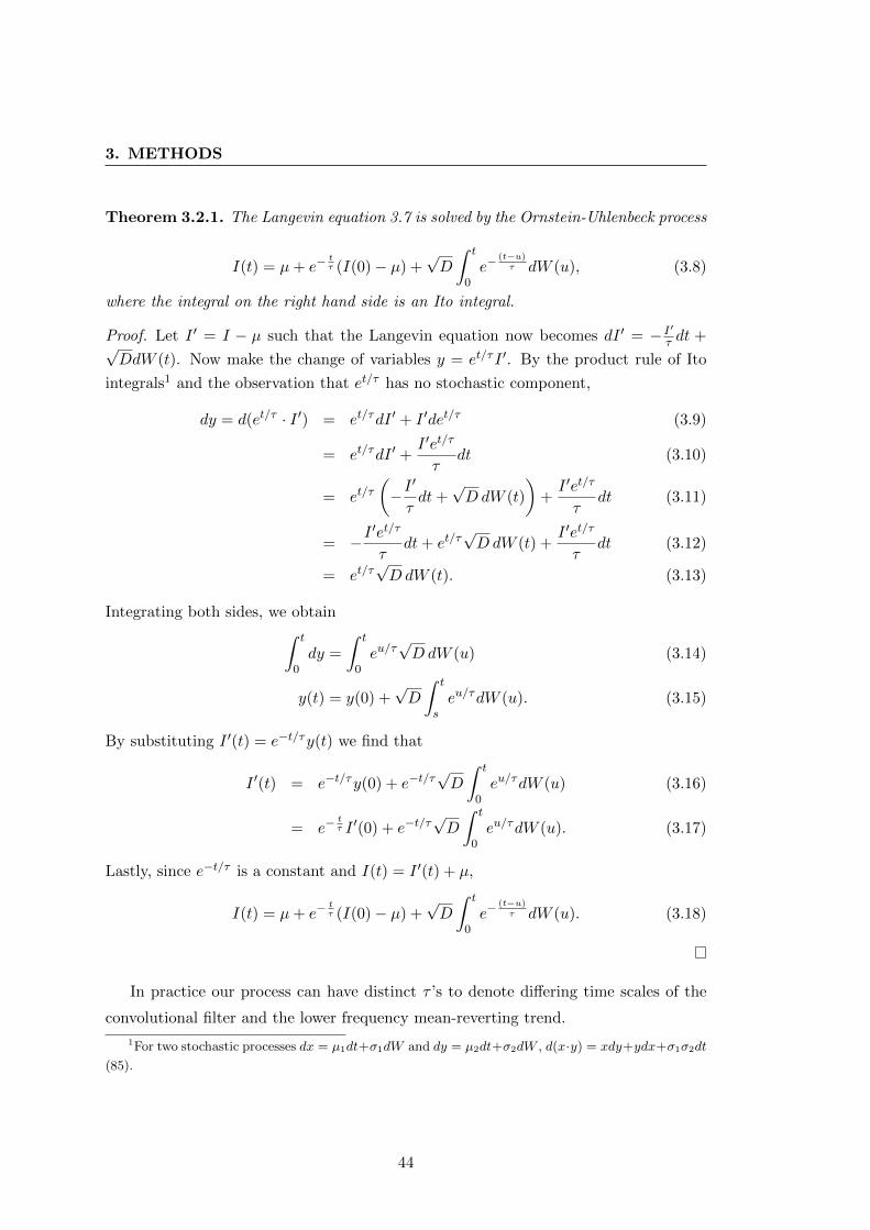
3. METHODS

Theorem 3.2.1. The Langevin equation 3.7 is solved by the Ornstein-Uhlenbeck process

I(t) = µ+ e−tτ (I(0)− µ) +

√D

∫ t

0e−

(t−u)τ dW (u), (3.8)

where the integral on the right hand side is an Ito integral.

Proof. Let I ′ = I − µ such that the Langevin equation now becomes dI ′ = − I′

τ dt +√DdW (t). Now make the change of variables y = et/τI ′. By the product rule of Ito

integrals1 and the observation that et/τ has no stochastic component,

dy = d(et/τ · I ′) = et/τdI ′ + I ′det/τ (3.9)

= et/τdI ′ +I ′et/τ

τdt (3.10)

= et/τ(−I′

τdt+

√DdW (t)

)+I ′et/τ

τdt (3.11)

= −I′et/τ

τdt+ et/τ

√DdW (t) +

I ′et/τ

τdt (3.12)

= et/τ√DdW (t). (3.13)

Integrating both sides, we obtain∫ t

0dy =

∫ t

0eu/τ√DdW (u) (3.14)

y(t) = y(0) +√D

∫ t

seu/τdW (u). (3.15)

By substituting I ′(t) = e−t/τy(t) we find that

I ′(t) = e−t/τy(0) + e−t/τ√D

∫ t

0eu/τdW (u) (3.16)

= e−tτ I ′(0) + e−t/τ

√D

∫ t

0eu/τdW (u). (3.17)

Lastly, since e−t/τ is a constant and I(t) = I ′(t) + µ,

I(t) = µ+ e−tτ (I(0)− µ) +

√D

∫ t

0e−

(t−u)τ dW (u). (3.18)

In practice our process can have distinct τ ’s to denote differing time scales of the

convolutional filter and the lower frequency mean-reverting trend.

1For two stochastic processes dx = µ1dt+σ1dW and dy = µ2dt+σ2dW , d(x·y) = xdy+ydx+σ1σ2dt

(85).

44


3.2.3 Step Function

Since the step function is such a traditional tool of electrophysiology, we will also sim-

ulate the neuron’s response to this simple protocol, primarily as control to verify that

the neuron’s state should have zero information about such a process.

We assume that there are two sources of noise in this protocol: noise in the time

when the current steps on and noise in the current step’s amplitude. We then define

the current to be

I(t) =

{0 if t < Ton

k + σ1ξ if t ≥ Ton, (3.19)

where k ∈ R is some constant current, ξ ∼ N(0, 1), and Ton ∼ N(µ, σ22).

We show the neuron spiking in response to this choice of protocol in figure 3.2.

0 100 200 300 400 500 600 700 800 900 1000−100

−50

0

50Membrane Voltage V(t); ensemble size = 1

Time (ms)

Vo

lta

ge

(m

V)

0 100 200 300 400 500 600 700 800 900 1000−100

0

100

200Adaptation variable w(t); a = 8

Time

Ad

ap

tatio

n v

aria

ble

0 100 200 300 400 500 600 700 800 900 10000

500

1000Driving input: I

Time

Cu

rre

nt

(pA

)

Figure 3.2: Voltage V and adaptation variable w of the adapting (a = 8) exponential

integrate-and-fire neuron to 1 second of stimulation by a step current.

45

3. METHODS

3.3 Choice of State s(t)

This thesis focuses on the information processing inefficiencies of model neurons, which

requires computing the mutual information between the neuron’s input and the neuron’s

state. For the results in (4) to apply, our system states must change from st to st+δt

according to the transition probability p(st+δt | st, xt+δt), where x is the input current.

Since the transition probability only depends on the previous state and the current

input value, this is equivalent to the Markov assumption. This implies that we should

define the neuron’s state in such a way that it depends solely on its previous state and

the current input value. If we look at our model in terms of difference equations,

V (t+ δt) = V (t) +1

C

[f(V (t))− w(t) + I(t+ δt)

](3.20)

w(t+ δt) = w(t) +1

τw

[a(V (t)− EL)− w(t)

](3.21)

we can see that if s(t) =

[V (t)w(t)

]we can write our neuron model in a form that satisfies

these requirements. In particular, we would have

s(t+ δt) = s(t) +Ws(t) + g(s(t), I(t+ δt)) (3.22)

where W =

[−gL/C −1/Ca/τw −1/τw

]and g(s(t), I(t+ δt)) is

[1C

(I(t+ δt) + gL∆T exp

(eT1 s(t)−VT

∆T

)+ gLEL

)−aEL/τw

], (3.23)

and eT1 = [1 0].

In practice, the information in w(t) about the stimulus I(t) is almost entirely cap-

tured by the voltage, since w determines the state of adaptation which is reflected in

the number of spikes present in V (t). While there is some inherent ambiguity in the

meaning of a spike as the state of adaptation changes, experimental studies suggest that

information to resolve this ambiguity is nonetheless present in the temporal sequence

of spikes alone (41).

46

3.4 What is a Neuron in Equilibrium?

3.4 What is a Neuron in Equilibrium?

In treating our model neuron as a physical system, there are several issues we need to

address before we can expect to understand the neuron’s thermodynamics of predic-

tion. For one, the neuron must be surrounded by a heat bath such that temperature is

well-defined. In reality this may not be such a wild notion, since neurons are suspended

in matrices of intercellular fluid, blood vasculature, and surrounding tissue.

Even more importantly, we need to define what it means for the neuron’s state s(t)

to be in thermodynamic equilibrium. In order for us to apply the thermodynamics of

prediction, we must have a system that is driven from its equilibrium by our choice of

protocol I(t). In the absence of this protocol (or equivalently, for fixed I(t) = 0), the

equilibrium distribution of system states is given by the Boltzmann distribution

peq(s | I = 0) =1

Ze−βE(s, I=0), (3.24)

where E(s, I = 0) is the total energy of the system in state s and Z is the partition

function

Z =∑s

e−βE(s, I=0). (3.25)

The model neuron can be represented by a fairly simple RC circuit, with resistors and

capacitors in parallel. In this circuit, the cell membrane separates charges resulting in a

capacitance C, while the conductances of ion channels embedded in the membrane de-

termine the neuron’s resistance (13). At steady state when there is zero input current,

this resistance is given solely by the conductance gL of the non-voltage gated channels

called leak channels (13).

We compute the model neuron’s thermodynamic equilibrium at input current I(t) = 0.

Since our neuron at equilibrium is in steady state, we must have

a(V − EL)− w = τwdw

dt= 0, (3.26)

which must be true for all values of a ∈ R. At this point we restrict ourselves to calcu-

lating the equilibrium at time t = 0 before any adaptation occurs; i.e., the adaptation

variable is zero. These conditions leave us no choice but for the steady state voltage to

47

3. METHODS

be V = EL.

In the absence of input current, there must be no current leaving the circuit by Kir-

choff’s law, which states that the sum of currents flowing into and out of a given node

must be zero. Then no current is flowing across the resistor or capacitor, and all of the

energy in the circuit must be stored as stationary charge on the capacitor. The energy

stored on the capacitor is equal to the energy needed (or equivalently, the work done)

to charge it. If the membrane separates a positive charge +q on one side and −q on the

other, then moving a small charge dq from one side to the other against the potential

difference V = q/C (2.1.1) requires energy dE,

dE = V dq =q

Cdq, (3.27)

which we can then integrate over the entire charge Q on the capacitor,

E =

∫ Q

0

q

Cdq =

1

2

Q2

C=

1

2CV 2. (3.28)

Since our potential difference is EL at steady state, with a simple change of variables

the total energy E stored on our membrane capacitor is then

E(V ) =1

2C(V − EL)2. (3.29)

Substituting our total energy in 3.24 we then have the equilibrium distribution of states

peq(V ) =1

Ze−

βC(V−EL)2

2 =1

Ze− (V−EL)2

2(1/βC) . (3.30)

Noting the similarity this bears to the normal distribution

f(x) =1

σ√

2πe−

(x−µ)2

2σ2 , (3.31)

we conclude that peq(V ) must be normally distributed with variance 1/βC and mean

EL. Recalling that β = 1kBT

, where kB is the Bolzmann constant, we have peq(V ) ∼N(EL,

kBTC ). For our implementation, we assume average core human body temperature

T = 310 K (86), and capacitance C = 281 pF as per Table 3.1.

48

4

Results

To investigate the role of adaptation in the thermodynamic and information theoretic

efficiency of neurons, we simulated large ensembles of adaptive exponential integrate-

and-fire neurons responding to various stimuli with differing temporal correlations. We

then computed the mutual information between the state of the neuron at time t and

either the stimulus at time t (instantaneous memory) or the stimulus at time t + δt

(instantaneous predictive power).

If st and xt are our neuron state and stimulus, respectively, at time t, and τ is the

length of our stimulus, then the total memory Imem =∑τ−1

t=0 I(st;xt) and total predic-

tive power Ipred =∑τ−1

t=0 I(st;xt+1) determine a lower bound on the neuron’s average

dissipation (4),

β〈Wdiss〉 ≥ Imem − Ipred. (4.1)

This has the tremendous implication that systems with nonzero memory like the model

neuron must be predictive about the future stimulus in order to operate efficiently.

Real neurons are thought to adapt in order to better encode a stimulus without sat-

urating its limited operating range or wasting spikes to continue communicating an

unchanging stimulus (87, 88, 89, 90, 91). Building on this long history of efficient cod-

ing, we make the stronger claim that adaptation maximizes both the total memory

and predictive power of the neuron model. Furthermore, by utilizing the nonequilib-

rium thermodynamics result 4.1 we can make concrete predictions about the energy

49

4. RESULTS

efficiency of neurons across both adapting and non-adapting neurons. Lastly, we find

that peak memory and predictive information occurs when the time scale of adaptation

matches that of the stimulus.

4.1 Adaptation Maximizes Memory and Predictive Power

In the classic efficient coding paradigm (87, 92), adaptation maximizes the mutual in-

formation between the stimulus and the neural response. Similarly, we find that for

the adaptive exponential integrate-and-fire neuron model this quantity is largest in the

regime where it adapts to the stimulus (figure 4.1).

Despite having lower firing rates than non-adapting neurons (left inset in figure 4.1),

the information the neuron carries about the stimulus steadily increases with the adap-

tation parameter a. Eventually, a becomes large enough that the voltage is continually

hyperpolarized by the adaptation variable w(t) and so no longer spikes, even to strong

stimuli. In this regime, the advantage of adaptation is lost and the memory capacity

of the neuron decreases as the hyperpolarization strengthens.

Surprisingly though, when the stimulus has nonzero temporal correlations, the vast

majority - over 99.7% - of the neuron’s information about the stimulus is predictive

information (figure 4.1). This implies that the dynamics of the model neuron are suf-

ficient to almost only capture information about the present that generalizes to the

future.

4.2 Neurons Are Energy Efficient Across All Adaptation

Regimes

While the neuron’s efficiency as measured in bits per spike is higher when the neuron

is adaptable, we found that the neuron’s minimum theoretical energy dissipation was

virtually constant for all degrees of adaptation (figure 4.1).

Since dissipation is constant throughout periods of high firing and low firing (figure 4.1),

action potentials must be highly efficient despite being energetically expensive (26).

50

4.2 Neurons Are Energy Efficient Across All Adaptation Regimes

0 5 10 15 20 250

1000

2000

3000

4000

5000

6000

7000

8000

9000Sum of Memory, Predictive power, and Nonpredictive information

Sum

of b

its o

ver 1

000

ms

Adaptation parameter a

red − nonpredictive information

cyan − total memory

blue − predictive power

green − total memory in the protocol

Adaptation Regimeadaptation regime

green : upper bound on Ipred

cyan : Imem

blue : Ipred

red : Imem � Ipred

Figure 4.1: Total Memory, Predictive Power, and Nonpredictive information as a function

of adaptation. Here we quantify the sum of instantaneous memory, predictive power,

and nonpredictive information of the adaptive exponential integrate-and-fire neuron model

being driven out of equilibrium by one second of the Ornstein-Uhlenbeck stimulus. Insets

are example voltage traces for a neuron with (from left to right) a = 0, 6, and 20 responding

to a simple step of current.

Over the 1 second protocol length, the system accumulated on average roughly 13

bits of nonpredictive information Imem − Ipred. Using the inequality 4.1 and the av-

erage core body temperature of T = 310.65 K, the average energy dissipated by the

neuron over one second is

〈Wdiss〉 = kBT (Imem − Ipred) = 13kBT (4.2)

≈ 6× 10−20 J. (4.3)

51

4. RESULTS

Since the average firing rate was close to 4 Hz, this constitutes only about 2 × 10−20

J of dissipation per action potential. Compared to the estimated metabolic cost of

3.8 × 10−11 J per action potential (26), this amounts to an inefficiency of losing only

one part in two billion to dissipation. This result buttresses recent experimental find-

ings that the parameters of action potentials (93) and ion channels (37) are tuned for

energy efficiency.

Figure 4.2: Instantaneous memory (blue), predictive power (green), nonpredictive infor-

mation (red), and the total information available in the stimulus (grey). Bottom plots are

spike rasters. The leftmost panes capture the high spiking behavior of a non-adapting neu-

ron, the middle panes correspond to an adapting neuron (a = 6), and the rightmost panes

correspond to a non-spiking neuron. In low noise conditions, the analog neuron captures

the most information about the stimulus yet is the most inefficient.

We also found that the generation of action potentials generated less dissipation than

an analog neuron that carries information about the stimulus solely through its sub-

threshold potential (figure 4.2). Although the subthreshold potential encoded stimulus

values continuously, resulting in a higher memory and predictive information capacity,

its instantaneous nonpredictive information was substantially higher than that of any

spiking neuron (figure 4.2).

52

5

Discussion

For decades sensory neurons have been conceptualized as maximizing information about

their stimulus (87, 92, 94, 95) while minimizing energetic cost (6, 26, 37). Moreover,

adaptation is thought to be the primary mechanism that allows neurons to actively

achieve both of these goals (87, 88, 89, 90, 91). Adaptation to a static stimuli will

conserve spikes while there is no information to convey, and, since neurons have a fixed

dynamic range, adapting to the particular mean and variance of a stimulus prevents

the neural response from saturating at either low or high firing rates.

Here we show that adaptation not only maximizes a neuron’s memory about its stim-

ulus, but also that almost all of this memory about the stimulus is predictive of the

future stimulus value. From this observation that the model neuron does not keep any

nonpredictive information, we applied the recent far-from-equilibrium thermodynamics

result from (4) to show that the spiking dynamics of neurons are incredibly energy

efficient compared to the cost of a single action potential.

Since this claim of efficiency is a lower bound on the energy dissipation of real or

in silica neurons, it remains to be shown how close to this new theoretical minimum

real neurons approach.

53

References

[1] R. Landauer. Computation: A fundamental physi-

cal view. Physica Scripta, 35:88, 1987. 1, 29

[2] S. Lloyd. Computational capacity of the universe.

Physical Review Letters, 88(23):237901, 2002. 1

[3] G. Neske. The notion of computation is fundamen-

tal to an autonomous neuroscience. Complexity,

16(1):10–19, 2010. 1

[4] Susanne Still, David A Sivak, Anthony J Bell, and Gavin E

Crooks. Thermodynamics of prediction. Physical Re-

view Letters, 109(12):120604, 2012. 1, 2, 3, 5, 23, 24, 27,

30, 31, 38, 46, 49, 53

[5] F. Rieke. Spikes: exploring the neural code. The MIT

Press, 1999. 1, 6

[6] S.B. Laughlin, R.R.R. van Steveninck, and J.C. Anderson.

The metabolic cost of neural information. Nature

neuroscience, 1(1):36–41, 1998. 2, 8, 53

[7] G.H. Recanzone, M.M. Merzenich, and C.E. Schreiner.

Changes in the distributed temporal response

properties of SI cortical neurons reflect improve-

ments in performance on a temporally based tac-

tile discrimination task. Journal of Neurophysiology,

67(5):1071–1091, 1992. 2

[8] F. Rieke and DA Baylor. Single-photon detection by

rod cells of the retina. Reviews of Modern Physics,

70(3):1027, 1998. 2

[9] Eric R Kandel, James H Schwartz, and Thomas M Jessell.

Principles of neural science. McGraw-Hill, Health Pro-

fessions Division, New York, 4th ed edition, 2000. 2, 4,

6, 7

[10] Peter Dayan and L. F Abbott. Theoretical neuroscience:

computational and mathematical modeling of neural sys-

tems. Massachusetts Institute of Technology Press, Cam-

bridge, Mass., 2001. 4

[11] R.W. Williams and K. Herrup. The control of neuron

number. Annual Review of Neuroscience, 11(1):423–453,

1988. 5

[12] D.A. Drachman. Do we have brain to spare? Neurol-

ogy, 64(12):2004–2005, 2005. 5

[13] Philip S. Ulinski. Fundamentals of Computational

Neuroscience. Unpublished Manuscript, 2010. 5, 7, 9,

47

[14] R. Yuste. Circuit neuroscience: the road ahead.

Frontiers in neuroscience, 2(1):6, 2008. 5

[15] A.J. Bell. Towards a cross-level theory of neural

learning. In 27th international workshop on Bayesian

inference and maximum entropy methods in science and

engineering, AIP Conference Proceedings, 954, pages 56–

73, 2007. 5

[16] S.M. Sherman and RW Guillery. Functional organiza-

tion of thalamocortical relays. Journal of Neurophys-

iology, 76(3):1367–1395, 1996. 5

[17] G. Laurent and H. Davidowitz. Encoding of olfac-

tory information with oscillating neural assem-

blies. Science, 265(5180):1872–1875, 1994. 5

[18] P.S. Churchland and T.J. Sejnowski. Perspectives on

cognitive neuroscience. Science, 242(4879):741–745,

1988. 6

[19] J. Gautrais and S. Thorpe. Rate coding versus tem-

poral order coding: a theoretical approach. Biosys-

tems, 48(1-3):57–65, 1998. 6

[20] R.V. Rullen and S.J. Thorpe. Rate coding versus

temporal order coding: what the retinal gan-

glion cells tell the visual cortex. Neural computation,

13(6):1255–1283, 2001. 6

[21] V. Booth and A. Bose. Neural mechanisms for gener-

ating rate and temporal codes in model CA3 pyra-

midal cells. Journal of neurophysiology, 85(6):2432–

2445, 2001. 6

[22] J. Huxter, N. Burgess, and J. OKeefe. Independent rate

and temporal coding in hippocampal pyramidal

cells. Nature, 425(6960):828, 2003. 6

[23] MR Mehta, AK Lee, and MA Wilson. Role of experience

and oscillations in transforming a rate code into

a temporal code. Nature, 417(6890):741–746, 2002. 6

[24] Bertil Hille. Ionic channels of excitable membranes.

Sinauer Associates, Sunderland, Mass., 2nd ed edition,

1992. 6, 7, 9, 10

[25] J.W. Mink, R.J. Blumenschine, and D.B. Adams. Ratio

of central nervous system to body metabolism

in vertebrates: its constancy and functional ba-

sis. American Journal of Physiology-Regulatory, Inte-

grative and Comparative Physiology, 241(3):R203–R212,

1981. 8

[26] J.E. Niven and S.B. Laughlin. Energy limitation as a

selective pressure on the evolution of sensory sys-

tems. Journal of Experimental Biology, 211(11):1792–

1804, 2008. 8, 50, 52, 53

[27] L. Stryer. Biochemistry. W.H. Freeman and Company,

5th edition edition, 2002. 8

[28] P.W. Hochachka and G.N. Somero. Biochemical adapta-

tion: mechanism and process in physiological evolution.

Oxford University Press, USA, 2002. 8

[29] HB Barlow. Trigger features, adaptation and econ-

omy of impulses. Information Processing in the Nervous

System, pages 209–230, 1969. 8

54

http://www.loc.gov/catdir/description/mh023/99044479.html

http://www.loc.gov/catdir/toc/fy031/2001044005.html



REFERENCES

[30] W.B. Levy and R.A. Baxter. Energy efficient neural

codes. Neural Computation, 8(3):531–543, 1996. 8

[31] D.J. Field. What is the goal of sensory coding?

Neural computation, 6(4):559–601, 1994. 8

[32] Michael S Gazzaniga. The cognitive neurosciences. MIT

Press, Cambridge, Mass., 4th ed edition, 2009. 8

[33] B.A. Olshausen and D.J. Field. Sparse coding of

sensory inputs. Current opinion in neurobiology,

14(4):481–487, 2004. 8

[34] A.A. Faisal, J.A. White, and S.B. Laughlin. Ion-channel

noise places limits on the miniaturization of the

brains wiring. Current Biology, 15(12):1143–1149,

2005. 8

[35] L.C. Aiello and P. Wheeler. The expensive-tissue hy-

pothesis: the brain and the digestive system in

human and primate evolution. Current anthropology,

36(2):199–221, 1995. 8

[36] P. Achard and E. De Schutter. Complex parameter

landscape for a complex neuron model. PLoS Com-

putational Biology, 2(7):e94, 2006. 8

[37] A. Hasenstaub, S. Otte, E. Callaway, and T.J. Sejnowski.

Metabolic cost as a unifying principle govern-

ing neuronal biophysics. Proceedings of the National

Academy of Sciences, 107(27):12329, 2010. 8, 52, 53

[38] E.M. Izhikevich. Simple model of spiking neurons.

Neural Networks, IEEE Transactions on, 14(6):1569–

1572, 2003. 8, 39

[39] G. Fuhrmann, H. Markram, and M. Tsodyks. Spike fre-

quency adaptation and neocortical rhythms. Jour-

nal of neurophysiology, 88(2):761–770, 2002. 8, 9

[40] A.L. Fairhall, G.D. Lewen, W. Bialek, and

RR de Ruyter van Steveninck. Multiple timescales

of adaptation in a neural code. Advances in neural

information processing systems, pages 124–130, 2001. 9

[41] A.L. Fairhall, G.D. Lewen, W. Bialek, and R.R.

de Ruyter van Steveninck. Efficiency and ambiguity

in an adaptive neural code. Nature, 412(6849):787–

792, 2001. 9, 41, 46

[42] J. Benda and A.V.M. Herz. A universal model for

spike-frequency adaptation. Neural computation,

15(11):2523–2564, 2003. 9

[43] I.A. Fleidervish, A. Friedman, and MJ Gutnick. Slow in-

activation of Na+ current and slow cumulative

spike adaptation in mouse and guinea-pig neocor-

tical neurones in slices. The Journal of physiology,

493(Pt 1):83–97, 1996. 9

[44] W. Gerstner and R. Naud. How good are neuron mod-

els? Science, 326(5951):379–380, 2009. 9

[45] LF Abbott et al. Lapicques introduction of the

integrate-and-fire model neuron (1907). Brain re-

search bulletin, 50(5):303–304, 1999. 9

[46] W. Gerstner and W.M. Kistler. Spiking neuron models:

Single neurons, populations, plasticity. Cambridge Univ

Pr, 2002. 10

[47] A.L. Hodgkin and A.F. Huxley. A quantitative de-

scription of membrane current and its application

to conduction and excitation in nerve. Bulletin of

mathematical biology, 52(1):25–71, 1990. 10

[48] E.M. Izhikevich. Dynamical systems in neuroscience: the

geometry of excitability and bursting. The MIT press,

2007. 10

[49] Romain Brette and Wulfram Gerstner. Adaptive ex-

ponential integrate-and-fire model as an effective

description of neuronal activity. J Neurophysiol,

94(5):3637–42, Nov 2005. 11, 39, 42

[50] C. Mead. Analog VLSI and neural systems. Addison-

Wesley Longman Publishing Co., Inc., 1989. 11

[51] G. Indiveri, B. Linares-Barranco, T.J. Hamilton,

A. Van Schaik, R. Etienne-Cummings, T. Delbruck,

S.C. Liu, P. Dudek, P. Hafliger, S. Renaud, et al. Neu-

romorphic silicon neuron circuits. Frontiers in

neuroscience, 5, 2011. 11, 12

[52] G. Indiveri. A low-power adaptive integrate-and-

fire neuron circuit. In Circuits and Systems, 2003. IS-

CAS’03. Proceedings of the 2003 International Symposium

on, 4, pages IV–820. Ieee, 2003. 11, 12, 39

[53] S.F. Zornetzer. An introduction to neural and electronic

networks. Academic Pr, 1995. 11

[54] C. Mead. Neuromorphic electronic systems. Pro-

ceedings of the IEEE, 78(10):1629–1636, 1990. 11

[55] J. Dethier, P. Nuyujukian, C. Eliasmith, T. Stewart,

S.A. Elassaad, K.V. Shenoy, and K. Boahen. A Brain-

Machine Interface Operating with a Real-Time

Spiking Neural Network Control Algorithm. Ad-

vances in Neural Information Processing Systems (NIPS)

24, 2011. 12

[56] S. Kim, P. Tathireddy, R.A. Normann, and F. Solzbacher.

Thermal impact of an active 3-D microelectrode

array implanted in the brain. Neural Systems

and Rehabilitation Engineering, IEEE Transactions on,

15(4):493–501, 2007. 12

[57] C. E. Shannon. A mathematical theory of commu-

nication. SIGMOBILE Mob. Comput. Commun. Rev.,

5(1):3–55, January 2001. 13

[58] Claude Elwood Shannon and Warren Weaver. The math-

ematical theory of communication. University of Illinois

Press, Urbana, 1949. 13

[59] T. M. Cover and Joy A Thomas. Elements of information

theory. Wiley-Interscience, Hoboken, N.J., 2nd ed edi-

tion, 2006. 16, 18, 19

[60] A. Dembo, T.M. Cover, and J.A. Thomas. Informa-

tion theoretic inequalities. Information Theory, IEEE

Transactions on, 37(6):1501–1518, 1991. 19

[61] J. R Norris. Markov chains. Cambridge University Press,

Cambridge, UK, 1st pbk. ed edition, 1998. 19

[62] G.E. Crooks. Excursions in statistical dynamics. PhD

thesis, UNIVERSITY of CALIFORNIA, 1999. 20, 25,

26

55

http://doi.acm.org/10.1145/584091.584093

http://doi.acm.org/10.1145/584091.584093

http://www.loc.gov/catdir/enhancements/fy0624/2005047799-d.html

http://www.loc.gov/catdir/enhancements/fy0624/2005047799-d.html

http://www.loc.gov/catdir/description/cam028/96031570.html

REFERENCES

[63] Christopher Jarzynski. Nonequilibrium work rela-

tions: foundations and applications. The European

Physical Journal B - Condensed Matter and Complex Sys-

tems, 64(3-4):331–340, 2008. 20, 21, 26

[64] Sadi Carnot. Reflexions sur la Puissance Motrice du Feu

et sur les Machines propres a Developper cette Puissance.

1824. 20

[65] A. Magnus. Quaestiones Alberti de modis significandi.

Benjamins, 1977. 21

[66] G.E. Crooks. Nonequilibrium measurements of free

energy differences for microscopically reversible

Markovian systems. Journal of Statistical Physics,

90(5):1481–1487, 1998. 22, 26

[67] R. Shaw. The dripping faucet as a model chaotic

system. 1984. 22

[68] E.M.F. Curado and C. Tsallis. Generalized statisti-

cal mechanics: connection with thermodynamics.

Journal of Physics A: Mathematical and General, 24:L69,

1991. 22

[69] E.T. Jaynes. Information theory and statistical me-

chanics. The Physical Review, 106(4):620–630, May 15

1957. 27, 29

[70] E.T. Jaynes. Information theory and statistical me-

chanics. II. Physical review, 108(2):171, 1957. 27

[71] R. Landauer. Irreversibility and heat generation in

the computing process. IBM journal of research and

development, 5(3):183–191, 1961. 29

[72] R. Landauer. The physical nature of information.

Physics letters A, 217(4-5):188–193, 1996. 29

[73] Bard Ermentrout and David H Terman. Mathematical

foundations of neuroscience, v. 35 of Interdisciplinary

applied mathematics. Springer, New York, 2010. 40

[74] E.P. Simoncelli and B.A. Olshausen. Natural image

statistics and neural representation. Annual review

of neuroscience, 24(1):1193–1216, 2001. 41

[75] C.F. Stevens, A.M. Zador, et al. Input synchrony and

the irregular firing of cortical neurons. Nature neu-

roscience, 1(3):210–217, 1998. 42

[76] G. Svirskis and J. Rinzel. Influence of temporal corre-

lation of synaptic input on the rate and variability

of firing in neurons. Biophysical journal, 79(2):629,

2000. 42

[77] N.A. Hessler, A.M. Shirke, and R. Malinow. The proba-

bility of transmitter release at a mammalian cen-

tral synapse. 1993. 42

[78] A. Destexhe and D. Pare. Impact of network activity

on the integrative properties of neocortical pyra-

midal neurons in vivo. Journal of Neurophysiology,

81(4):1531–1547, 1999. 42

[79] Laurence O Trussell, Su Zhang, and Indira M Ra-

mant. Desensitization of AMPA receptors upon

multiquantal neurotransmitter release. Neuron,

10(6):1185–1196, 1993. 42

[80] Z.F. Mainen and T.J. Sejnowski. Reliability of

spike timing in neocortical neurons. Science,

268(5216):1503–1506, 1995. 42

[81] Paul Horowitz and Winfield Hill. The art of electronics.

Cambridge University Press, Cambridge, 2nd ed edition,

1989. 42

[82] G.E. Uhlenbeck and L.S. Ornstein. On the theory of the

Brownian motion. Physical Review, 36(5):823, 1930.

43

[83] A. Destexhe, M. Rudolph, J.M. Fellous, and T.J. Se-

jnowski. Fluctuating synaptic conductances recre-

ate in vivo-like activity in neocortical neurons.

Neuroscience, 107(1):13–24, 2001. 43

[84] G. La Camera, M. Giugliano, W. Senn, and S. Fusi. The

response of cortical neurons to in vivo-like input

current: theory and experiment. Biological cybernet-

ics, 99(4):279–301, 2008. 43

[85] L.C. Evans. An introduction to stochastic differen-

tial equations. lecture notes, Department of Mathemat-

ics, University of California, Berkeley. http://www. math.

berkeley. edu/˜ evans/SDE. course. pdf, 2002. 44

[86] D. Fiala, K.J. Lomas, and M. Stohrer. Computer pre-

diction of human thermoregulatory and temper-

ature responses to a wide range of environmen-

tal conditions. International Journal of Biometeorology,

45(3):143–159, 2001. 48

[87] Simon B Laughlin. A simple coding procedure en-

hances a neurons information capacity. Z. Natur-

forsch, 36(910-912):51, 1981. 49, 50, 53

[88] Martin Stemmler and Christof Koch. How voltage-

dependent conductances can adapt to maximize

the information encoded by neuronal firing rate.

Nature neuroscience, 2(6):521–527, 1999. 49, 53

[89] Naama Brenner, William Bialek, and Rob de Ruyter van

Steveninck. Adaptive rescaling maximizes informa-

tion transmission. Neuron, 26(3):695–702, 2000. 49,

53

[90] Barry Wark, Brian Nils Lundstrom, and Adrienne

Fairhall. Sensory adaptation. Current opinion in neu-

robiology, 17(4):423–429, 2007. 49, 53

[91] Xaq Pitkow and Markus Meister. Decorrelation and

efficient coding by retinal ganglion cells. Nature

neuroscience, 15(4):628–635, 2012. 49, 53

[92] Joseph J Atick. Could information theory pro-

vide an ecological theory of sensory processing?

Network: Computation in neural systems, 3(2):213–251,

1992. 50, 53

[93] Henrik Alle, Arnd Roth, and Jorg RP Geiger. Energy-

efficient action potentials in hippocampal mossy

fibers. Science, 325(5946):1405–1408, 2009. 52

[94] Horace B Barlow. Possible principles underlying the

transformation of sensory messages. Sensory com-

munication, pages 217–234, 1961. 53

[95] Yang Dan, Joseph J Atick, and R Clay Reid. Efficient

coding of natural scenes in the lateral geniculate

nucleus: experimental test of a computational

theory. The Journal of Neuroscience, 16(10):3351–3362,

1996. 53

56

http://www.loc.gov/catdir/description/cam023/89000468.html

Information Processing and Energy Dissipation in Neurons

Documents

Transcript of Information Processing and Energy Dissipation in Neurons