San Jose State University San Jose State University

SJSU ScholarWorks SJSU ScholarWorks

Master's Projects Master's Theses and Graduate Research

2009

Information Flow Model for Commercial Security Information Flow Model for Commercial Security

Jene Pan San Jose State University

Follow this and additional works at: https://scholarworks.sjsu.edu/etd_projects

Part of the Computer Sciences Commons

Recommended Citation Recommended Citation Pan, Jene, "Information Flow Model for Commercial Security" (2009). Master's Projects. 72. DOI: https://doi.org/10.31979/etd.rp3r-2647 https://scholarworks.sjsu.edu/etd_projects/72

This Master's Project is brought to you for free and open access by the Master's Theses and Graduate Research at SJSU ScholarWorks. It has been accepted for inclusion in Master's Projects by an authorized administrator of SJSU ScholarWorks. For more information, please contact scholarworks@sjsu.edu.

Information Flow Model for Commercial Security

Final Writing Project

Presented to

The Faculty of the Department of Computer Science

San Jose State University

In Partial Fulfillment

of the Requirements for the Degree

Master of Science

by

Jene Pan

December 2009

APPROVED FOR THE DEPARTMENT OF COMPUTER SCIENCE Dr. Tsau Y. Lin, Department of Computer Science Date Dr. Suneuy Kim, Department of Computer Science Date Dr. Howard Ho, IBM Corporation Date

CS298 Report

Abstract Information flow in Discretionary Access Control (DAC) is a well-known

difficult problem. This paper formalizes the fundamental concepts and

establishes a theory of information flow security. A DAC system is

information flow secure (IFS), if any data never flows into the hands of

owner’s enemies (explicitly denial access list.)

- 1 -

CS298 Report

Table of Contents

1. INTRODUCTION...................................................................................... 4

2. CONCEPT OF SECURITY................................................................. 4

3. CONCEPT OF GRANULAR COMPUTING .......................... 5

3.1 FIRST MODEL (LOCAL GRC MODEL - NEIGHBORHOOD SYSTEM) ........ 7 3.2 THIRD MODEL (BINARY GRC MODEL – BINARY NEIGHBORHOOD SYSTEM)........................................................................................................................ 7

4. DISCRETIONARY ACCESS CONTROL (DAC)................ 9

4.1 GEOMETRIC VIEWS OF DAC....................................................................... 10

5. INFORMATION FLOW SECURITY ON DAC..................... 11

5.1 ILLUSTRATIONS.............................................................................................. 11 5.2 MAIN THEOREMS........................................................................................... 23

5.2.1 Example........................................................................................................ 24 5.3 CHINESE WALL SECURITY POLICY (CWSP) ............................................. 27 5.4 PROGRAMMATIC ILLUSTRATION................................................................. 28

5.4.1 Structure....................................................................................................... 29 5.4.2 Algorithm ..................................................................................................... 31 5.4.3 Testing results............................................................................................. 34 5.4.4 Illustration of application........................................................................ 35

6. CONCLUSION ................................................................................................... 40

6.1 HISTORICAL NOTES ON THE METHODOLOGY........................................... 40 6.2 FUTURE WORK................................................................................................ 41

7. REFERENCES................................................................................................... 42

- 2 -

CS298 Report

Table of Figures

Figure 1. Partition is a very neat granulation...................................................................... 5 Figure 2. Trajectory of object A, T(A) ............................................................................. 12 Figure 3. Geometric view of T(A) .................................................................................... 13 Figure 4. Trajectory of object B , T(B)............................................................................. 13 Figure 5. Geometric view of T(B) .................................................................................... 14 Figure 6. Trajectory of object C, T(C).............................................................................. 14 Figure 7. Geometric view of T(C) .................................................................................... 14 Figure 8. Trajectory of object D, T(D) ............................................................................. 15 Figure 9. Geometric view of T(D) .................................................................................... 15 Figure 10. Trajectory of object E, T(E) ............................................................................ 15 Figure 11. Geometric view of T(E)................................................................................... 16 Figure 12. Screen 1 of Programmatic view of example 1................................................. 16 Figure 13. Screen 2 of Programmatic view of example 1................................................. 17 Figure 14. Trajectory of object A, T(A) ........................................................................... 18 Figure 15. Geometric view of T(A) .................................................................................. 18 Figure 16. Trajectory of object B, T(B)............................................................................ 18 Figure 17. Geometric view of T(B) .................................................................................. 19 Figure 18. Trajectory of object C, T(C)............................................................................ 19 Figure 19. Geometric view of T(C) .................................................................................. 19 Figure 20. Trajectory of object D, T(D) ........................................................................... 20 Figure 21. Geometric view of T(D) .................................................................................. 20 Figure 22. Trajectory of object E, T(E) ............................................................................ 20 Figure 23. Geometric view of T(E)................................................................................... 21 Figure 24. The failure of Information Flow Security Policy of object E.......................... 21 Figure 25. Programmatic view of example 2.................................................................... 22 Figure 26. Trajectory of object A ..................................................................................... 25 Figure 27. Trajectory of object B...................................................................................... 25 Figure 28. Trajectory of object C...................................................................................... 26 Figure 29. Trajectory of object D ..................................................................................... 26 Figure 30. Trajectory of object E...................................................................................... 26 Figure 31. A Geometric view of all 5 objects in set O ..................................................... 27 Figure 32. Input file .......................................................................................................... 29 Figure 33. Output file........................................................................................................ 31 Figure 34. Start application............................................................................................... 35 Figure 35. Import Input file .............................................................................................. 36 Figure 36. Notification of completion of analyzing process............................................. 36 Figure 37. Four buttons available for retrieving information and analysis result............. 37 Figure 38. The given E List in input file........................................................................... 37 Figure 39. MF List (the complement) of the given E List ................................................ 38 Figure 40. T List of the given E List................................................................................. 38 Figure 41. Final result of information flow analysis......................................................... 39

- 3 -

CS298 Report

1. Introduction

Computer technology has been advanced greatly in the recent years. With technology growth, faster and cheaper computers are widely available to the users. Needless to say, these big leaps in technology have greatly improved our efficiency and effectiveness; nonetheless, they also pose a serious challenge in maintaining adequate data security. Commercial security systems take the following view: A system is considered to be “secure” if an individual user has the authority to allow or deny access to the data that he owns. Its formal model is the so-called the discretionary access control model (DAC). In this model, users are called subjects, and data are called objects. However, it has been known for a long time that access control of information on Discretionary Access Control system is a difficult problem. A discretionary access control (DAC) model is, well, at the discretion of the owner of data. An object’s owner has discretionary authority over who else may access that object. DAC, however, does not deal with information flow, and discretionary usually means anyone with access can propagate information. With this model, it is often criticized that discretionary access control cannot prevent the illegitimate propagation once access is granted. In this report, we will formalize the fundamental concepts and establish the theory of information flow security on discretionary access control system. As a consequence we have solved information propagation via granular computing. 2. Concept of security Common definition of computer security is: a system is secure if it adequately protects information that it processes against the followings:

a. Unauthorized disclosure b. Unauthorized modification c. Deny of service

In this report, we are addressing information flow security. So, item a is the only relevant one. In military security, the department of the defense (DoD) is the sole agent who decides the authorization. However, in UNIX, the owner of the data is the agent to authorize who can access his data; for simplicity, we shall call those

- 4 -

CS298 Report

who have been authorized the friends (access control list with abbr. ACL). In practice, by default, those who are not in ACL are enemies. In this paper, we will sharpen the relevant concepts. An enemy is the one to whom the owner has absolute objection for accessing his data. In military security, enemy list is the so-called explicitly denied access list. The concept of enemy list is stronger than the default in UNIX SYSTEM. So, we will discuss three lists for each user

1) E-list: enemy list 2) F-list: friend list 3) MF-list: the complement of E-list

By definition, E-list and F-list are disjoint, and F-list is subset of MF-list. Theoretically, we deal with MF-list. The closest concept to the UNIX’s friend list (ACL) is F-list

3. Concept of Granular computing Informally, Granular computing (GrC) is a computing theory based on granulation; A classical granulation is partition:

Figure 1. Partition is a very neat granulation

The term granular computing (GrC) was coined by Dr. Lin and Zadeh in Fall, 1996 [59]. However the idea can be traced back to [39]. Both Zadeh and Lin have basically adopted mathematical approach to GrC. Zadeh stated [58]:“Basically, TFIG… its foundation and methodology are mathematical in nature”. The word “TFIG”, abbreviation of theory of fuzzy information granulation, is precisely the granular computing (GrC).

- 5 -

CS298 Report

Having adopted incremental approach, Dr. Lin has accumulated nine GrC models. They are:

• First GrC Model (Local Granular Model) • Second GrC Model (Global Granular Model) • Third GrC Model (Binary Granular Model) • Fourth GrC Model (Multi-Binary Granular or Binary Granular Data

Model) • Fifth GrC Model (Relational Granular Model) • Sixth GrC Model • Seventh GrC Model • Eighth GrC Model (Categorical Granular Model) • Ninth GrC Model

In these nine models, the Eighth GrC Model, with its higher level view, is considered as the formal model of granulation, and the rest of them are basically “convenient models” as they all can be derived from the Eighth by specifying the general category to various special cases. We would like to quote the informal definition and formal definition from [57]. Zadehs informal definition: “information granulation involves partitioning a class of objects (points) into granules, with a granule being a clump of objects (points) which are drawn together by some constraints or forces, such as ‘indistinguishability, similarity or functionality”. “Intuitively, a class of objects that are drawn by some constraints forms a tuple with these constraints as the schema of the tuple. Let CAT be a given category Lin’s formal definition on Category Theory Based GrC Model:

1. Let C={Cjh | h ∈ H and j ∈ Jh } be a family of objects in the Category

CAT; it is called the universe (of discourse). 2. Consider a family Π of product objects in C 3. Consider a family β of relation objects, which are subobjects of Π.

Then the pair (C, β) is the “final” Formal GrC Model that has been called the Category Theory Based GrC Model (also 8th GrC Model). Remark: Note that if CAT is the category of sets, then we can regard C as the union of these sets Cj

h. “ From the Eighth model, if we specify the category to the category of sets, we have the Fifth model. This model is a collection of n-relations or n-tuples in the view of relational database schema. From this model, the First and Fourth models are formed if the product objects are limited to be the product of 2 objects. The First model is referred to neighborhood system (NS), and the Fourth is a multi-binary model. If all n-ary relations in the Fifth model are

- 6 -

CS298 Report

symmetric, the Second model is formed. However, a granule in the Second model has to be a set, and a granule in the Fifth model can be a tuple and may not be a set. The Third model is built if the number of binary relations is reduced to be one. This model is referred to be binary neighborhood (BNS). Because BNS is a special case of NS, the Third model is a special case of the First model. The Sixth, the Seventh, and the Ninth are derived directly from the Eighth model depending on how the category is taken category. If category is taken to be the category of fuzzy sets, functions, random variables and generalized functions, we form the Sixth model. If category is taken to be the category of Turing machines, we form the Seventh model. If category is taken to be the category of qualitative fuzzy sets, we form The Ninth model. In this report, we only concern with the Third model, binary neighborhood system (BNS). As BNS is special case of NS (neighborhood system), we shall discuss the First model (Local GrC) and Third (Binary GrC) model in more details.

3.1 First Model (Local GrC Model - Neighborhood System) “The theory of neighborhood systems is abstracted from the geometric notion of ‘near’ or ‘negligible distances’." [16]. For each point p in the universe U, one associates with it a family of subsets. This family may or may not be empty, and each subset in the family is NS(p) and is called a neighborhood system at p or a neighborhood at p respectively. A neighborhood system of the universe U, denoted as NS(U), is the collection β of that kind of a family at every element or point p of the universe. In granular computing, Neighborhood and neighborhood system are called granule and the granular structure respectively. Let β be NS, the pair (U, β) will be a local granular model as each granule is associated with some points. We use Dr. Lin’s words to give the formal definition for this model [57] Definition “First GrC Model: The 3-tuple (V,U,β) is called Local GrC Model, where β is a neighborhood system (NS). If V = U, the 3-tuple is reduced to a pair (U, β). In addition, if we require NS to satisfy the topological axioms, then it becomes a TNS.”

3.2 Third Model (Binary GrC Model – Binary Neighborhood System)

The type of neighborhood system arises from binary relation is called binary neighborhood system. Let U and V be the two classical sets. With a subset R of Cartesian product V × U is a binary relation, we will re-express R by binary granulation [17].

- 7 -

CS298 Report

A binary relation defines a mapping B, called binary granulation for each p of the set V as: B : V → 2U : p → B(p), where B(p) = {u | (p, u) ∈ R} Conversely, given B, we can define the binary relation R, which is a set of ordered pairs (p, u) from a set Bp, a power set of the set U, to a set V as: R = {(p, u) | u ∈ Bp∀ p ∈ V} The defining of B(p) = {u | (p, u) ∈ R} is a right neighborhood, and the collection B of B(p) at each p of V is the (right) binary neighborhood system (BNS). Similarly, a left version is defined as: a left neighborhood system L is defined by the set of L(p) where L(p) = {u | (u, p) ∈ R} at every p of V. The Third model is the pair (U, β) where β is R or right (left) neighborhood system. This model arises from a binary relation, so it is called a binary granular model. Dr. Lin gives the definition for the model as follows: [57] Definition: “3rd GrC model is the three-tuple (U, V, β), where β is a BNS. It may be referred to as a binary GrC model. If U = V, then the three-tuple is reduced to a pair (U, β). Observe that BNS is equivalent to a BR:

BR = {(p, Y ) | Y ∈ B(p) and p ∈ V}. Conversely, a BR defines a (right) BNS as follows:

p → B(p) = {Y | (p, Y ) ∈ BR} So both modern examples give rise to BNS, which was called a binary GrS in Lin (1998a). We would like to note that based on this (right) BNS, the (left) BNS can also be defined:

D(p) = {Y | p ∈ B(Y ) for all p ∈ V }.“ In computer security, Discretionary Access Control Model (DAC) assigns each user p a family of users, Yi, i = 1, 2, 3, …, who can access p’s data. In other words, each p is assigned a granule of friends. To formalize DAC model, let U and V be two classical sets. Each p∈ V is assigned a subset B(p) of “basic knowledge”. This knowledge is a set of friends or a “neighborhood” of positions.

p → B(p) = {Yi, i = 1, 2, … } ⊆ U In this model, such a set B(p) is called a right binary neighborhood, and the collection { B(p) | ∀ p ∈ V} is called the binary neighborhood system (BNS) In granular computing point of view, DAC is a binary neighborhood system. We will examine DAC in more details in section 4.

- 8 -

CS298 Report

4. Discretionary Access Control (DAC)

We will formulate UNIX’s ACL based on BN’s language. In 1989, Brewer and Nash (abbreviated, BN) proposed a very interesting security policy, called Chinese wall security policy [2]. The paper essentially addresses the information flow problem on DAC. So we will use its notations and language, to formulate the idea of UNIX-permission-bits in terms of the concepts of information flow on DAC. A user in UNIX is the owner of an account. Without the lost of generality, we will refer the files in an account that have the same permission bits as the dataset of the account, owned by a company. BN referred the dataset of a company as an object. So the UNIX-permission-bits essentially specify a group of users who can access the information of an object, say X. Here the access means to read and may be to save the information of X to the datasets of this group. We will abstract such an access to a concept of information flow. We say information in object X has flowed into an object Y when this type of an access occurs. Here, Y is a generic object in the group. We have taken pains to abstract the UNIX files into objects. However, the notion of objects shall not be restricted to UNIX. Abstractly, an object consists of information (dataset) and its container (the account). So, information in a DAC can flow from an object and can be received by objects. Following BN, we will denote the collection of all those objects to be the set O. Therefore, the permission bits are abstracted to the following: To each object, say X ∈ O, we associate a group F(X) = {Yj, j = 1, 2, …} of objects who may receive information from X. In other words, information in X may flow into any object Yj, j = 1, 2, …. The set F(X) is often referred to as the access control list (ACL). We will call it the friend-list of X. Similarly, the enemy-list of X, denoted by E(X), consists of a group of objects, to which no information of X can be flowed to or from X directly. This list has been referred to as explicitly denied list [23]. Definition 1 Discretionary Access Control Model (DAC) is a map

F : O → 2O : X → F(X). that associates each object of O with a group of friends, called friend-list. 2O, known as the power set of O, denotes the collection of all subsets of O. In this report, we will denote this DAC by F-DAC. Here, F is used to emphasize that the information is flowed into friends' datasets. By analogy, we can define the following:

- 9 -

CS298 Report

Definition 2 E-DAC model is a map

E : O → 2O : X → E(X). that associates each object of set O with a group of enemies, called an enemy-list. Such a list has been called explicitly denied list [23]. Abstractly, the friend-list F(X) and the enemy-list E(X) concern the "same" concept (see the geometric discussions below.) Let Y be an object that information of X is allowed to flow into, in other words, Y ∈ F(X). We will denote this permissibility by X ⇒ Y. Observe that the collection of the pairs (X, Y) related by X ⇒ Y is a subset of Cartesian product O x O. Hence, a binary relation is defined. Definition 3 The set {(X, Y) | Y ∈ F(X)} is a binary relation, denoted by F or more graphically ⇒. This binary relation is called Direct Information Flow Model (DIF). Similarly, {(X, Y) | Y ∈ E(X)} is a binary relation, denoted by E. From these definitions, it is clear that we have the following proposition. Proposition 1 F-DAC and F are equivalent. Similarly, E-DAC and E are equivalent. By abuse of notations, F and E will denote both F-DAC and E-DAC and the respectively corresponding binary relations.

4.1 Geometric Views of DAC The concept of F(X) and E(X) can be viewed geometrically: Let U be a set and p be a point in U. Here, U is a geometric view of O. We shall consider the geometric abstraction of F-DAC or E-DAC. Namely, Definition 1 Geometric abstraction of F-DAC (or E-DAC) is a map B : U → 2U : p → B(p) that associates each point p of U with a subset B(p). This map is called a binary neighborhood system (BNS) or a binary granulation. B(p), called a neighborhood, is the geometric abstraction of F(X). By abuse of language, we will also call the collection {B(p) | p ∈ U} a BNS. Definition 2 Let O be the set of all objects, and X an object.

- 10 -

CS298 Report

T(X) = F( X) ∪ F[F[X]] ∪ F[F[F[X]]] … (transfinitely many) is called the trajectory of information flows from X.

5. Information Flow Security on DAC The nature of the information flow is "continuously flowing." So we need to trace its trajectories, namely, we have to apply ⇒ repeatedly to the objects. So we define: Definition 1 Information Flow from X to Y is defined to be the compositions of finite sequences of ⇒ (Direct information flow): X = {X0 ⇒ X1 ⇒ X2 … ⇒ Xn = Y} Here, n varies through integers. Note that this includes the case, X ⇒ X. The collection of such (X, Y) is a reflexive binary relation, denoted by C and called Information Flow Model. Corollary 1 C is the transitive closure of F. The following corollary is immediate from the definition. Corollary 2 T(X) = {Y | (X, Y ) ∈ C} Intuitively, T(X) consists of all possible points that the information flows are allowed to reach. The central theme of this report is to discuss: How the DAC can be designed properly so that Main Theme Information flows can never flow into enemies' hands. Formally, we say T(X) ∩ E(X) = ∅ ∀ X ∈ O. Definition 2 The requirement that information flows will never flow into enemy list is called information flow security policy (IFSP). As a result, if T(X) meets IFSP, we will denote such T(X) as ST(X) and call it the secure trajectory information flows from X. We have ST(X) = MF(X), and F(X) ⊆ ST(X) if F(X) is not maximal.

5.1 Illustrations

Let us illustrate the concept by examples:

- 11 -

CS298 Report

Example 1 (Positive example): Assume we have a set O that contains five objects A, B, C, D, E and their E-DAC is given below: A → E { } B → E {A} C → E {A, B} D → E {A, B, C} E → E {A, B, C, D} By default, we assume the complement of each friend-list is an enemy-list. Therefore, each friend-list (F) is also its maximal friend-list (MF) and F-DAC is: A → {A, B, C, D, E} B → {B, C, D, E} C → {C, D, E} D → {D, E} E → {E} In this example, the F-DAC is secure in the sense that no information of an object X may flow into its enemies' objects. Let us look at the trajectory of each object A ⇒ A ⇒ B => C ⇒ D ⇒ E T(A) = {A, B, C, D, E} does not meet E(A) = { } T(A) meets IFSP; therefore, T(A) = ST(A)

A

DB

E

C

Figure 2. Trajectory of object A, T(A)

- 12 -

CS298 Report

A B C D E

A B C D E

A B C D E

A B C D E

A B C D E

A B C D E

Figure 3. Geometric view of T(A) B ⇒ B ⇒ C ⇒ D ⇒ E T(B) = {B, C, D, E} does not meet E(B) = {A} T(B) meets IFSP; therefore, T(B) = ST(B)

B

DA

E

C

Figure 4. Trajectory of object B , T(B)

- 13 -

CS298 Report

Figure 5. Geometric view of T(B) \ C ⇒ C ⇒ D ⇒ E T(C) = {C, D, E} does not meet E(C) = {A, B} T(C) meets IFSP; therefore, T(C) = ST(C)

Figure 6. Trajectory of object C, T(C)

Figure 7. Geometric view of T(C)

A B C D E

A B C D E

A B C D E

A B C D E

A B C D E

C

DA

E

B

A B C D E

A B C D E

A B C D E

A B C D E

- 14 -

CS298 Report

D ⇒ D ⇒ E T(D) = {D, E} does not meet E(D) = {A, B, C} T(D) meets IFSP; therefore, T(D) = ST(D)

D

CA

B

E

Figure 8. Trajectory of object D, T(D)

A B C D E

A B C D E

A B C D E

Figure 9. Geometric view of T(D) E ⇒ E T(E) = {E} does not meet E(E) = {A, B, C, D} T(E) meets IFSP; therefore, T(E) = ST(E)

EB

C

D

A

Figure 10. Trajectory of object E, T(E)

- 15 -

CS298 Report

A B C D E

A B C D E

Figure 11. Geometric view of T(E)

So information in every object can never flow into the enemies.

Figure 12. Screen 1 of Programmatic view of example 1

- 16 -

CS298 Report

Figure 13. Screen 2 of Programmatic view of example 1

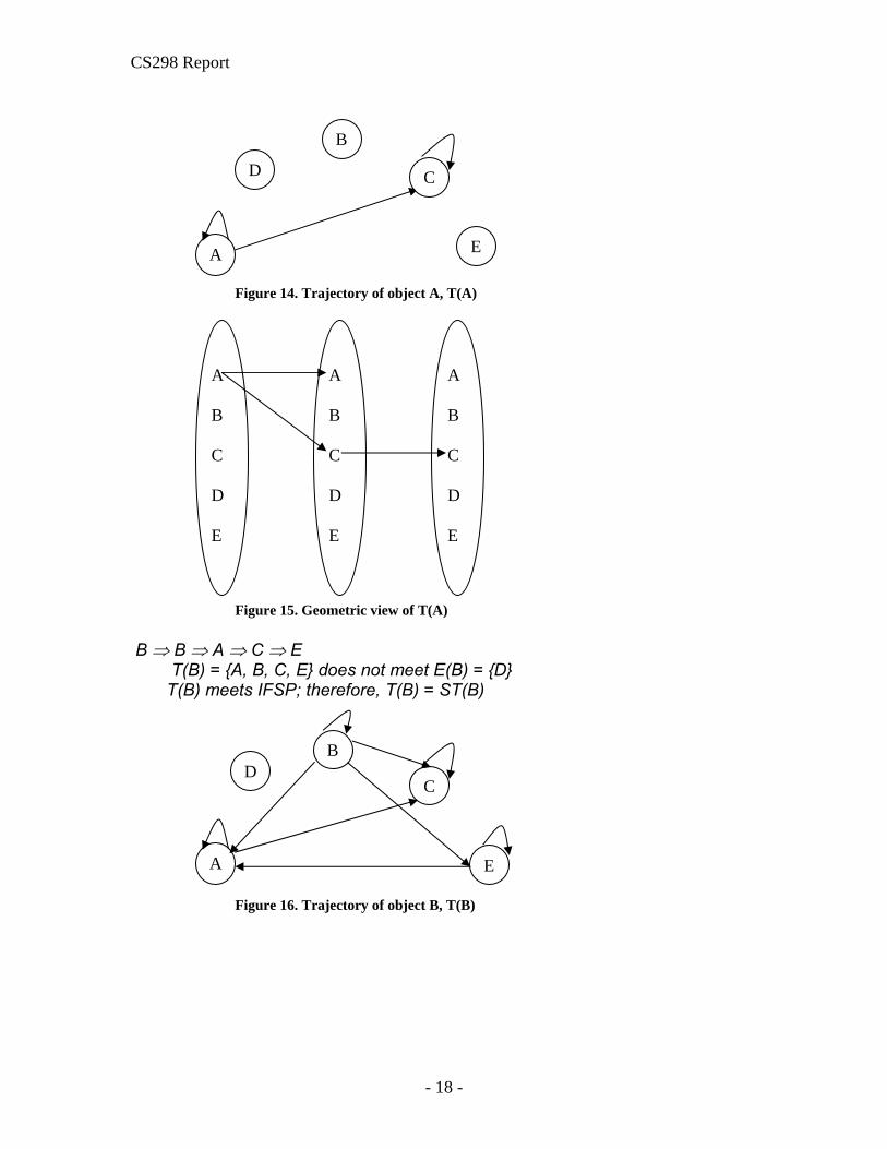
Next,let us look at a negative example. Example 2 (Negative example): The enemy lists are: A → E {B, D, E} B → E {D} C → E {A, B, D, E} D → E {A, B, C, E} E → E {B, C, D} By default, the friend-lists (F) again same as maximal friend-lists (MF) are: A → {A, C} B → {A, B, C, E} C → {C} D → {D} E → {A, E} Now, observe that the trajectories are: A ⇒ A ⇒ C T(A) = {A, C} does not meet E(A) = {B, D, E}

T(A) meets IFSP; therefore, T(A) = ST(A)

- 17 -

CS298 Report

A

CD

E

B

Figure 14. Trajectory of object A, T(A)

A B C D E

A B C D E

A

B

C

D

E

Figure 15. Geometric view of T(A) B ⇒ B ⇒ A ⇒ C ⇒ E

T(B) = {A, B, C, E} does not meet E(B) = {D} T(B) meets IFSP; therefore, T(B) = ST(B)

A

CD

B

E

Figure 16. Trajectory of object B, T(B)

- 18 -

CS298 Report

A B C D E

A B C D E

A B C D E

Figure 17. Geometric view of T(B) C ⇒ C T(C) = {C} does not meet E(C) = {A, B, D, E} T(C) meets IFSP; therefore, T(C) = ST(C)

A

C

D

E

B

Figure 18. Trajectory of object C, T(C)

A

B C D E

A B C D E

Figure 19. Geometric view of T(C)

- 19 -

CS298 Report

D ⇒ D T(D) = {D} does not meet E(D) = {A, B, C, E} T(D) meets IFSP; therefore, T(D) = ST(D)

Figure 20. Trajectory of object D, T(D)

Figure 21. Geometric view of T(D) E ⇒ E ⇒ A ⇒ C T(E) = {A, C, E} does meet E(E) = {B, C, D} T(E) does not meet IFSP; therefore, T(E) ≠ ST(E)

Figure 22. Trajectory of object E, T(E)

A CE

B

D

A B C D E

A B C D E

D

C

E

B

A

- 20 -

CS298 Report

A B C D E

A B C D E

A B C D E

A B C D E

Figure 23. Geometric view of T(E)

E B

A D

C

T(E) E(E)

T(E) ∩ E(E) ≠ ∅

Figure 24. The failure of Information Flow Security Policy of object E

These phenomena occur because F-DAC does not satisfy the Information Flow Security conditions.

- 21 -

CS298 Report

Figure 25. Programmatic view of example 2

- 22 -

CS298 Report

5.2 Main Theorems

Let us recall some definitions 1. A symmetric binary relation B is a binary relation such that for every (u, v)

∈ B implies (v, u) ∈ B. 2. B’ = V × V ~ B, which is the complement set of B, defines the complement

binary relation (CBR). 3. A binary relation B is anti-reflexive if B is non-empty and no pair (v, v) is in

B. Observed that B is anti-reflexive iff (if and only if) B' is reflexive. 4. A binary relation B is anti-transitive if B is non-empty and if (u, v) belongs

to B implies that for all w either (u, w), (w, v) or both belongs to B. Observed that B is anti-transitive iff B' is transitive.

Let us examine the main theorem, which can be viewed as a generalization of Chinese wall security theorem [22]. Theorem 1 Information Flow Security Theorem. E-DAC enforces information flow security policy if E-DAC is anti-transitive This will follow directly from the following corollary. Proposition Information Flow Security Theorem. Let F-DAC be the complement of E-DAC, then E-DAC enforces information flow security policy if F-DAC is transitive Observe that since F-DAC is transitive, the trajectories stay in F(X). So, T(X) is disjoint from E(X), and hence it satisfies IFSP. Next we re-state the Chinese Wall Security Theorem in terms of IFSP. We quote two important statements from BN: 1. "The Chinese wall security policy combines commercial discretion with legally enforceable mandatory controls . . . , perhaps, as significant to the financial world as Bell-LaPadula's policies are to the military." See for Bell-LaPadula's policies 2. "People are only allowed access to information which is not held to conflict with any other information that they already possess." See [2], Section "Simple Security", p. 207. Simple Chinese wall security policy implies that F-DAC is an equivalence relation:

- 23 -

CS298 Report

1. We observe that if two datasets are accessible by the same agent, we should conclude that the information of two datasets can be flowed into each others

2. From the second assertion of BN, we conclude that an agent can access any information that is not in conflict with the information they already possess. So in F(X), which is outside of E(X), all information can flow into each other. Hence F-DAC is an equivalence relation.

So we define: Definition 1. Simple Chinese wall security policy (SCWSP) means F-DAC is an

equivalence relation. 2. Aggressive Chinese wall security policy (ACSWP) means C is an

equivalence relation. Theorem 2 Chinese Wall Security Theorem. Simple Chinese wall security policy implies Aggressive Chinese wall security policy. This is immediate: C is an equivalence relation if and only if F is. Corollary Simple Chinese Wall Security Policy (SCWSP) implies IFSP. This is immediate: since equivalence relation is transitive. Equivalence relation is a special case of binary relation. F-DAC in the Third GrC model is a binary relation, and F-DAC in Chinese wall model is an equivalence relation. Therefore, Chinese wall model is a special case of Information flow model.

5.2.1 Example Example 3 Assume we have a set O with five objects A, B, C, D, E and their E-DAC is given below: A → E {B, D, E} B → E {A, C, E} C → E {B, D, E} D → E {A, C, E} E → E {A, B, C, D} By default, we assume the complement of each friend-list is an enemy-list. Therefore, each friend-list (F) is also its maximal friend-list (MF) and F-DAC is: A → {A, C} B → {B, D}

- 24 -

CS298 Report

C → {A, C} D → {B, D} E → {E} In this example, the F-DAC is secure in the sense that no information of an object X may flow into enemies' objects. Let us look at the trajectory of each object A ⇒ C ⇒ A

T(A) = {A, C} does not meet E(A) = {B, D, E} T(A) meets IFSP; therefore, T(A) is ST(A)

CA

B

D

E

Figure 26. Trajectory of object A B ⇒ D ⇒ B T(B) = {B, D} does not meet E(B) = {A, C, E} T(B) meets IFSP; therefore, T(B) is ST(B)

DB

A

C

E

Figure 27. Trajectory of object B C ⇒ A ⇒ C

T(C) = {A, C} does not meet E(C) = {B, D, E} T(C) meets IFSP; therefore, T(C) is ST(C)

- 25 -

CS298 Report

Figure 28. Trajectory of object C D ⇒ B ⇒ D

T(D) = {B, D} does not meet E(D) = {A, C, E} T(D) meets IFSP; therefore, T(D) is ST(D)

AC

B

D

E

BD

A

C

E

Figure 29. Trajectory of object D

E ⇒ E T(E) = {E} does not meet E(E) = {A, B, C, D} T(E) meets IFSP; therefore, T(E) is ST(E)

EB

C

D

A

Figure 30. Trajectory of object E

- 26 -

CS298 Report

A C B D E

A C B D E

Figure 31. A Geometric view of all 5 objects in set O So, information in every object can never flow into the enemies. In the above graph, the double arrow line connecting a pair of different objects indicates symmetry. For example, a symmetry is between A and C, and other is between B and D. The red lines on the graph divide the set O into 3 disjoint subsets {A, C}, {B, D}, and {E}. This partition represents an equivalence relation, which is a special case of binary relation.

5.3 Chinese wall security policy (CWSP)

This model was proposed by Brewer and Nash in 1989. Intuitively, Chinese Wall Security Policy (CWSP) is a very intriguing commercial security model. The basis idea of CWSP is to build the walls between datasets in the same “conflict of interest class”, and people are only allowed to access to information in the same side of the wall. In other words, they are not allowed to access information that is in the same “conflict of interest class”. All company data are stored in a hierarchical filing system. This filing system contains three levels:

a. At the lowest level, we deal with individual items of information, each concerning a single company. We shall refer to the files in which such information is stored as objects.

b. At the intermediate level, all objects concerning the same company are

grouped together into what is called a company dataset.

- 27 -

CS298 Report

c. At the highest level, all company datasets whose companies are in competition are grouped together into what is called a conflict of interest class.

This policy combines commercial discretion with legally enforcement mandatory controls. There is no information flow from X to Y if and only if X and Y belong to the same “conflict of interest class”, or equivalently, information flows from X to Y if and only if X and Y are not in the same “conflict of interest class”.

For example, there are two “conflict of interest” classes on business about oil and bank. The first class contains four oil companies which are Oil-A, Oil-B, Oil-C, and Oil-D; the second contains three banks which are Bank-A, Bank-B, and Bank-C. As there is no conflict of interest between bank dataset and oil dataset, a user A, who has accessed to Bank-A dataset, can only request access to the dataset of an oil company, such as Oil-A, Oil-B, Oil-C, or Oil-D. He no longer has access to the dataset of either Bank-B or Bank-C since they are in same “conflict of interest” as Bank A. Similarly, once he gains access to an oil company, say Oil-A, he would no longer has access to any bank or oil company other than Bank-A and Oil-A.

5.4 Programmatic illustration To analyze the security of information flow for each object in the system, we build a window application to validate whether the system satisfies IFSP. The system is considered to be secure if every object in the system satisfies IFSP, i.e., the intersection of its E list and its T list equals to an empty set. This application works as follows:

a. Input: The application will read the E-DAC in the system from an input file. The file contains many rows. Each row in the file describes the E list of an object in the system.

b. Process: The application will compute the friend lists (denoted as MF lists). The MF notation is used to indicate the complement of E list and is the maximal friend list. The trajectory lists (denoted as T lists) will then be generated from MF lists for each object in the system. Based on T list and E list of an object, the application then validates whether the dataset of this object is satisfied the IFSP. The system is secure if the datasets of all objects in the system meet IFSP.

c. Output:

- 28 -

CS298 Report

The application will write the result of the analysis to an output file. The program takes O(n3) with the main design as follows:

5.4.1 Structure Input file: The input file describes the E-DAC for all objects in the system. Each row of the input file describes an E list of an object. Each row has the following format: E(A) = { B, D, E } This row defines the E list of object A to be the set containing objects B, D, and E. Sample input file:

Figure 32. Input file Data structure: Each object of the system has the following attributes:

a. ID: a unique identifier, which identifies each object in the system. b. enemyString: this is the enemy list of the object, described in a string.

A comma separates each enemy. This is basically the same format as the row in the input file.

c. E list: this is a hash table, which contains the entire enemy list of the object. Each entry in the hash table has a (key, value) pair. The key is an enemy object ID, and the value is a reference to an enemy object.

- 29 -

CS298 Report

d. MF list: this is a hash table, which stores the complement of E list. Similarly, each entry in the hash table has a (key, value) pair.

e. T list: this is a hash table, which stores the trajectory list of the object. Similarly, each entry in the hash table has a (key, value) pair.

f. I list: this is a linked list, which stores E ∩ T We will use a hash table to store all the objects in the system. Each entry in the hash table has a (key, value) pair. The key stores the object ID. The value stores the reference to the object itself. To make it easy to refer to this hash table later on, we will call this hash table the allObjects hash table.

Output file: The output file contains the result of our analysis. It contains the following sections:

a. Summary of the result of the analysis. b. Each object’s MF list, T list, I list, and whether its dataset is secure.

Sample output file:

- 30 -

CS298 Report

Figure 33. Output file

5.4.2 Algorithm Step 1: Initialize allObjects hash table from input file.

• Read input file, row by row • Construct an object, and parse each row to obtain the ID, the

enemyString for that object. • Store the object to allObjects hash table.

At the end of step 1, the allObjects hash table will contain all objects in

the system. Step 2: Build E list

- 31 -

CS298 Report

The E list of each object X is built as follows:

function buildEList() { Parse enemyString into a temporary array of object IDs, tmpIDarray. Traverse tmpIDarray { - Obtain a reference to an enemy object by looking up allObjects

hash table, using the object ID as key. - Put this reference to the E list hash table of object X. } } Step 3: Build MF list The MF list of each object X is built as follows: Function buildMFList() { - Make a copy of allObjects hash table called MF list - Traverse object X’s E list - Remove objects found in X’s E list from that MF list } Step 4: Build T list

The T list of each object X is built as follows:

function buildTList() { Object X: the examined object for which its T list is built Queue q: a temporary queue to hold all possible objects of T list Object curObject: an object in the queue q to be examined. // Observe: the maximum length of queue q is n for n objects or users. // Queue q only stores distinct objects or users. while (there is an item in the queue) {//The loop cannot be looped more than the total number of distinct

objects curObject := dequeue the 1st item in the queue q; foreach (object o in curObject’s MF list) { if (o is not in X’s T-list)

- 32 -

CS298 Report

{//This condition keeps q to store only distinct objects or users

Add object o to X’s T list; If o is not curObject: enqueue to place o into queue q } } } } Step 5: Build I list

The I list of each object X is built as follows: Function builtIList() { Traverse X’s E list Add object to X’s I list if object is found in X’s T list }

Step 4 is the most critical part of the application to achieve O(n3) performance. To avoid infinitely looping and minimize the run time, we ensure that the MF list of each possible object can only be visited once during the traversal process while building the T list. For easier understanding, let us go through the buildTList function, steps by steps, to build T list of object E in the following example: Example: the given enemy list, E-DAC as follows: A → E {B, D, E} B → E {A, C, E} C → E {B, D, E} D → E {A, C, E} E → E {B, C, D} We will have the complement of E-list, the maximal friend-list MF below: A → {A, C} B → {B, D} C → {A, C} D → {B, D} E → {E, A} 1. Place E in the queue.

- 33 -

CS298 Report

2. Enter while loop a. Since the queue contains E, E is dequeued. b. Enter foreach loop

i. Since MF list of E contains E and A, we will examine to see whether E’s T list contains E and A.

ii. Since E’s T list is initially empty, it does not contain E. Therefore, E is added to E’s T list.

iii. E will not be placed in the queue since it is the curObject, and its MF list is currently examined.

iv. A is added to E’s T list, since E’s T list does not contain A. v. A is also enqueued, since A is not the curObject.

c. Exit foreach loop. At this point, the queue has one object, which is A.

3. Re-enter while loop a. Since the queue contains A, A is dequeued. b. Enter foreach loop

i. Since MF list of A contains A and C, we will examine to see whether E’s T list contains A and C.

ii. Since E’s T list already contains A, nothing happens. iii. C is added to E’s T list, since E’s T list does not contain C. iv. C is also enqueued, since C is not the curObject.

c. Exit foreach loop. At this point, the queue has one object, which is C.

4. Re-enter while loop a. Since the queue contains C, C is dequeued. b. Enter foreach loop

i. Since MF list of C contains A and C, we will examine to see whether E’s T list contains A and C.

ii. Since E’s T list already contains A and C, nothing happens. c. Exit foreach loop. At this point, the queue is empty.

5. Exit while loop since the queue is now empty. 6. E’s T list is now completely built.

5.4.3 Testing results

We have done the test for all possible cases of 4 and 5 objects. The results are following: 1. Four objects

For IFSP: Total number of objects = 4 Total number of cases examined = 4096 Total number of 0 object secure = 699 Total number of 1 object secure = 1140

- 34 -

CS298 Report

Total number of 2 objects secure = 1098 Total number of 3 objects secure = 804 Total number of secure (all 4 objects are secure) = 355 For ACWSP: Total number of cases examined = 355 Total number of cases met CWSP requirement = 15

2. Five objects

For IFSP: Total number of objects = 5 Total number of cases examined = 1048576 Total number of 0 object secure = 412004 Total number of 1 object secure = 336210 Total number of 2 objects secure = 176980 Total number of 3 objects secure = 84720 Total number of 4 objects secure = 31720 Total number of secure (all 5 objects are secure) = 6942 For ACWSP: Total number of cases examined = 6942 Total number of cases met CWSP requirement = 52

5.4.4 Illustration of application

Figure 34. Start application

- 35 -

CS298 Report

Import input filename in Open Input File text box

Figure 35. Import Input file Click on Start Analysis button to run the application. The notification displays when the analysis is completed.

Figure 36. Notification of completion of analyzing process Click OK button to go back the application

- 36 -

CS298 Report

Figure 37. Four buttons available for retrieving information and analysis result Click on View Input Data Set button to see E list, the content of input file. For example of section 5.4.2 above, file input should be in the following format.

Figure 38. The given E List in input file Click on View Complement Set button to see MF list, the complement of E list.

- 37 -

CS298 Report

Figure 39. MF List (the complement) of the given E List Click on View Trajectory Set button to see T list.

Figure 40. T List of the given E List Click on View Result button to see the analysis of security state for the given E list.

- 38 -

CS298 Report

Figure 41. Final result of information flow analysis

- 39 -

CS298 Report

6. Conclusion

In this project, we address the most "ancient" problem in computer security. Propagation of information is vulnerable. With the information flow security policy, we are able to state that the propagation under most general theorem for a DAC can be secure. To ensure a DAC being secure, the minimum requirement of a system is to store not only the access control list (ACL) but also the denial access list. The access control list is considered as F-DAC, and the denial access list is considered as E-DAC.

6.1 Historical Notes on the methodology

Let us say few words about the history of the new methodology. The very first idea was started from David Hsiao, who is one of the initial members of the group of doing research on this field. I would like to take this chance to thank him for introducing the great idea of granulation. I would also like to take this opportunity to specially thank Dr. Lin for his guidance though out the course of the project. Our approach is essential based on a computational theory of granulation, called “granular computing”. It has originated from four facets. Let us speak in the chronological order. The first one is David Hsiao. In his attribute based database model, Hsiao clusters the attribute domain into semantically related granules (equivalence classes); Clustering (this is different from the same term in data mining) is a very important technique in database that stores logically related data in physical proximity [7, 8, 5, 15]. The second one, probably the deepest one, is actually buried in the design of fuzzy control systems. The explicit discussion of the concept is in the article [39]; its newest version is in [40]. The third groups are from theory of data. Both Z. Pawlak and T.T. Lee observed independently that attributes of a relation induce partitions on the set of entities [26, 10] and studied the data from such observation. Pawlak called it rough set theory, while Lee named it the algebraic theory of relational databases. The last one comes from approximate retrieval [24, 11, 4]. To develop a theory of approximate retrieval in database, Dr. Lin imported the notion of topology from the continuous world to the discrete world; he has called it neighborhood system, which can be viewed as a geometric (topological) theory of granulations [17, 18]. Having citing so many works, he notes that the notion of partitions (= equivalence relations) is a very ancient notion in mathematics. It can be dated back to Euclid time, for example, the congruence. The notion of infinitesimal granules can be traced back to Archimedes. Here, however, the focus is on the computable side of the notion; so the notion has been called “granular computing”. The methodology has been far reaching consequence, for

- 40 -

CS298 Report

example, there are applications to the foundation of database mining (e.g., association rules) [20, 21]. In earlier paper, he applies it to security, more precisely, on conflict analysis [27], which is an essential notion in commercial security.

6.2 Future work There is more work that could be continued on this research to achieve security on the future systems that are developed on DAC model.

1) Making minimal change to fulfill the information flow security policy (IFSP) for a given F-DAC that does not meet IFSP.

2) Improving efficiency of storing and retrieving large data.

3) Resolve the complexity of the process to define and to analyze all

possible 2(n-1)n cases for n objects in the system.

- 41 -

CS298 Report

7. References

[1] Bell, D. 1987. Secure computer systems: A network interpretation. In Proceedings on 3rd Annual Computer Security Application Conference. 32-39. [2] David D. C. Brewer and Michael J. Nash: "The Chinese Wall Security Policy" IEEE Symposium on Security and Privacy, Oakland, May, 1988, pp 206-214. [3] Richard A. Brualdi, Introductory Combinatorics, Prentice Hall, 1992. [4] W. Chu and Q. Chen Neighborhood and associative query answering, Journal of Intelligent Information Systems, 1, 355-382, 1992. [5] S. A. Demurjian and S. A. Hsiao "The Multimodel and Multilingual Database Systems-A Paradigm for the Studying of Database Systems, " IEEE Transaction on Software Engineering, 14, 8, (August 1988) [6] Denning, D. E. 1976. A lattice model of secure information flow. Commun. ACM 19,2, 236-243. [7] Hsiao, D.K., and Harary, F.,"A Formal System for Information Retrieval From Files," Communications of the ACM, 13, 2(February 1970). Corrigenda CACM 13,3 (March, 1970) [8] Wong, E., and Chiang, T. C., "Canonical Structure in Attribute-Based File Organization," Communications of the ACM, Vol. 14, No. 9, September 1971. [9] C. E. Landhehr, and C. L. Heitmeyer:Military Message Systems: Requirements and Security Model, NRL Memorandom Report 4925, Computer Science and Systemss Branch, Naval research Laboratory. [10] T. T. Lee, "Algebraic Theory of Relational Databases," The Bell System Technical Journal Vol 62, No 10, December, 1983, pp.3159-3204 [11] T. Y. Lin, Neighborhood Systems and Relational Database. In: Proceedings of 1988 ACM Sixteen Annual Computer Science Conference, February 23-25, 1988, 725 [12] "A Generalized Information Flow Model and Role of System Security Officer", Database Security: Status and Prospects II, IFIP-Transaction, edited by C. E. Landwehr, North Holland, 1989, pp. 85-103. [13] T. Y. Lin, Neighborhood Systems and Approximation in Database and Knowledge Base Systems, Proceedings of the Fourth International

- 42 -

CS298 Report

Symposium on Methodologies of Intelligent Systems, Poster Session, October 12-15, pp. 75-86, 1989. [14] T. Y. Lin, "Chinese Wall Security Policy - An Aggressive Model", Proceedings of the Fifth Aerospace Computer Security Application Conference, December 4-8, 1989, pp. 286-293. [15] "Attribute Based Data Model and Polyinstantiation," Education and Society, IFIP-Transaction, ed. Aiken, 12th Computer World Congress, September 7-11, 1992, pp.472-478. [16] T. Y. Lin, "Neighborhood Systems - A Qualitative Theory for Fuzzy and Rough Sets, "Advances in Machine Intelligence and Soft Computing, Volume IV. Ed. Paul Wang, 1997, Duke University, North Carolina, 132-155. ISBN:0-9643454-3-3 [17] T. Y. Lin "Granular Computing on Binary Relations I: Data Mining and Neigh-borhood Systems." In: Rough Sets In Knowledge Discovery, A. Skoworn and L. Polkowski (eds), Physica-Verlag, 1998, 107-121 [18] T. Y. Lin "Granular Computing on Binary Relations II: Rough Set Representations and Belief Functions." In: Rough Sets In Knowledge Discovery, A. Skoworn and L. Polkowski (eds), Physica - Verlag, 1998, 121-140. [19] T. Y. Lin "Chinese Wall Security Model and Conflict Analysis," the 24th IEEE Computer Society International Computer Software and Applications Conference (Compsac2000) Taipei, Taiwan, Oct 25-27, 2000 [20] T. Y. Lin "Feature Completion," Communication of IICM (Institute of Information and Computing Machinery, Taiwan) Vol 5, No. 2, May 2002, pp. 57-62. This is the proceeding for the workshop "Toward the Foundation on Data Mining" in PAKDD2002, May 6, 2002. [21] T. Y. Lin "A Theory of Derived Attributes and Attribute Completion," Proceedings of IEEE International Conference on Data Mining, Maebashi, Japan, Dec 9-12, 2002. [22] T. Y. Lin: Chinese Wall Security Policy Models: Information and Confining Trojan Horses. DBSec 2003: 275-287 [23] Teresa F. Lunt: Access Control Policies for Database Systems. DBSec 1988: 41-52

- 43 -

CS298 Report

[24] A, Motro: "Supporting Gaol Queries", in Proceeding of the First International Con-ference on Expert Database Systems, L. Kerschber (eds)m April 1-4, 1986, pp. 85-96. [25] S. Osborn, R. Sanghu and Q. Munawer," Configuring Role Based Access Control to Enforce Mandatory and Discretionary Access Control Policies," ACM Transaction on Information and Systems Security, Vol 3, No 2, May 2002, Pages 85-106. [26] Z. Pawlak, Rough sets. International Journal of Information and Computer Science 11, 1982, pp. 341-356. [27] Z. Pawlak, "On Conflicts," Int J. of Man-Machine Studies, 21 pp. 127- 134, 1984 [28] Z. Pawlak, Analysis of Conflicts, Joint Conference of Information Science, Research Triangle Park, North Carolina, March 1-5, 1997, 350- 352. [29] Polkowski, L., Skowron, A., and Zytkow, J., (1995),"Tolerance based rough sets." In: T.Y. Lin and A. Wildberger (eds.), Soft Computing: Rough Sets, Fuzzy Logic Neural Networks, Uncertainty Management, Knowledge Discovery, Simulation Councils, Inc. San Diego CA, 55-58. [30] Sandhu, R. S. Latticebased enforcement of Chinese Walls. Computer & Security 11, 1992, 753-763. [31] Sandhu, R. S. 1993. Lattice based access control models. IEEE Computer 26, 11, 9-19. [32] Sandhu,R.S.,Coyne,E.J.,Feinstein,H.L.,and Youman, C. E. 1996. Role based access control models. IEEE Computer 29, 2 (Feb.), 38 - 47. [33] Sandhu,R.AND Munawer, Q. 1998. How to do discretionary access control using roles. In Proceedings of the Third ACM Workshop on Role Based Access Control (RBAC '98, Fairfax, VA, Oct. 22{23), C. Youman and T. Jaeger, Chairs. ACM Press, New York, NY, 47-54. [34] W. Sierpinski and C. C, Kreiger, General Topology, University Toronto press, 1952 [35] T.C. Ting, “A User-Role Based Data Security Approach", in Database Security: Status and Prospects, C. Landwehr (ed.), North-Holland, 1988. [36] Demurjian, S., and Ting, T.C., "Towards a Definitive Paradigm for Security in Object-Oriented Systems and Applications," J. of Computer Security, Vol. 5, No. 4, 1997.

- 44 -

CS298 Report

[37] Liebrand, M., Ellis, H., Phillips, C., Demurjian, S., Ting, T.C., and Ellis, J., "Role Delegation for a Resource-Based Security Model," Data and Applications Security: Developments and Directions II, E. Gudes and S. Shenoi (eds.), Kluwer, 2003. [38] Phillips, C., Demurjian, S., and Ting, T.C., "Towards Information Assurance in Dynamic Coalitions," Proc. of 2002 IEEE Info. Assurance Workshop, West Point, NY, June 2002. [39] L.A. Zadeh, Fuzzy sets and information granularity, in: M. Gupta, R. Ragade, and R. Yager (Eds.), Advances in Fuzzy Set Theory and Applications, North-Holland, Amsterdam, 3-18, 1979. [40] L. Zadeh, "Some Reflections on Information Granulation and its Centrality in Granular Computing, Computing with Words, the Computational Theory of Perceptions and Precisiated Natural Language." In: T. Y. Lin, Y.Y. Yao, L. Zadeh (eds), Data Mining, Rough Sets, and Granualr Computing T. Y. Lin, Y.Y. Yao, L. Zadeh (eds) [41] Andrei Sabelfeld and Andrew C. Myers, "Language-Based Information-Flow Security," IEEE Journal on selected areas in communications, VOL. 21, No. 1, January 2003. [42] J. Todd Wittbold and Dale Johnson, “Information flow in nondeterministic systems.” In Proc. IEEE Symp. on Security and Privacy, pages 144–161, Oakland, CA, 1990. [43] S. Zdancewic and A. C. Myers, “Secure information flow via linear continuations,” Higher Order and Symbolic Computation, vol. 15, no. 2–3, pp. 209–234, Sept. 2002. [44] Andrew C. Myers and Barbara Liskov, "A Decentralized Model for Information Flow Control" In Proceedings of the 16th ACM Symposium on Operating Systems Principles (SOSP), pages 129-142, Saint-Malo, France, October 1997. [45] Andrew C. Myers, "JFlow: Practical Mostly-Static Information Flow Control" In Proceedings of the 26th ACM Symposium on Principles of Programming Languages (POPL ’99), San Antonio, Texas, USA, January 1999. [46] Neil Vachharajani, Mathew J. Bridges, Jonathan Chang, Ram Rangan, Guiherme Ottoni, Jason A. Blome, George A. Reis, Manish Vachharajani, David I. August, "RIFLE: An Architectural Framework for User-Centric Information-Flow Security" In Proceedings of the 37th annual IEEE/ACM

- 45 -

CS298 Report

International Symposium on Microarchitecture, pages 243-254, Portland, Oregon, 2004. [47] Matthew Hennessy and James Riely, "Information Flow vs. Resource Access in the Asynchronous Pi-Calculus”, ACM Transactions on Programming Languages and Systems (TOPLAS), Volume 24, No. 5, pages 566-591, September 2002. [48] Gavin Lowe, "Quantifying Information Flow”, Proc. IEEE Computer Security Foundations Workshop, 2002. [49] Massaaki Mizuno and David Schmidt, "A Security Flow Control Algorithm and Its Denotational Semantics Correctness Proof.” Formal Aspects of Computing 4, pages 727-754, 1992. [50] Gurvan Le Guernic and Thomas Jensen, "Monitoring Information Flow." Proc. Workshop on Foundations of Computer Security, 2005. [51] Peng Li and Steve Zdancewic, "Practical Information-flow Control in Web-based Information Systems" In Proceedings of the 18th IEEE Computer Security Foundations Workshop (CSFW), pages 2-15, 2005. [52] Peng Li and Steve Zdancewic, "Encoding Information Flow in Haskell." In Proceedings of the 19th IEEE Computer Security Foundations Workshop (CSFW), pages 16-27. IEEE Computer Society Press, 2006. [53] Steve Zdancewic, "Challenges for Information-flow Security" In Proceedings of the 1st International Workshop on the Programming Language Interference and Dependence (PLID’04), 2004. [54] Steve Zdancewic and Andrew C. Myers, "Secure Information Flow and CPS" In Proceedings of the 10th European Symposium on Programming (ESOP), volume 2028 of Lecture Notes in Computer Science, pages 46-61, April 2001. [55] Michael Dalton, Hari Kannan, Christos Kozyrakis, "Raksha A Flexible Information Flow Architecture for Software Security" In Proceedings of the 34th annual international symposium on Computer architecture, 2007. [56] Lantian Zheng and Andrew C. Myers, "Dynamic Security Labels and Static Information Flow Control" International Journal of Information Security, March 2007. [57] T. Y. Lin, "Granular computing I: the concept of granulation and its formal model" International Journal of Granular Computing, Rough Sets and Intelligent Systems, Vol. 1, No. 1, 2009.

- 46 -

CS298 Report

- 47 -

[58] Zadeh, L.A. (1997) ‘Toward a theory of fuzzy information granulation and its centrality in human reasoning and fuzzy logic’, Fuzzy Sets and Systems, Vol. 90, pp.111–127. [59] Zadeh, L.A. (1996) ‘The key roles of information granulation and fuzzy logic in human reasoning’, 1996 IEEE International Conference on Fuzzy Systems, New Orleans, Louisiana, 8–11 September 1996. [60] Tsau Young Lin: Granular Computing: Practices, Theories, and Future Directions. Encyclopedia of Complexity and Systems Science 2009: 4339-4355