Information Flow Analysis in Logical Form?

Torben Amtoft and Anindya Banerjee??

Department of Computing and Information SciencesKansas State University, Manhattan KS 66506, USA

{tamtoft,ab}@cis.ksu.edu

Abstract. We specify an information flow analysis for a simple impera-tive language, using a Hoare-like logic. The logic facilitates static check-ing of a larger class of programs than can be checked by extant type-basedapproaches in which a program is deemed insecure when it contains aninsecure subprogram. The logic is based on an abstract interpretationof program traces that makes independence between program variablesexplicit. Unlike other, more precise, approaches based on a Hoare-likelogic, our approach does not require a theorem prover to generate invari-ants. We demonstrate the modularity of our approach by showing thata frame rule holds in our logic. Moreover, given an insecure but termi-nating program, we show how strongest postconditions can be employedto statically generate failure explanations.

1 Introduction

This paper specifies an information flow analysis using a Hoare-like logic andconsiders an application of the logic to explaining insecure flow of informationin simple imperative programs.

Given a system with high, or secret (H), and low, or public (L) inputs andoutputs, where L ≤ H is a security lattice, a classic security problem is how toenforce the following end-to-end confidentiality policy: protect secret data, i.e.,prevent leaks of secrets at public output channels. An information flow analysischecks if a program satisfies the policy. Denning and Denning were the first toformulate an information flow analysis for confidentiality[12]. Subsequent ad-vances have been comprehensively summarized in the recent survey by Sabelfeldand Myers [28]. An oft-used approach for specifying static analyses for infor-mation flow is security type systems [24, 30]. Security types are ordinary typesof program variables and expressions annotated with security levels. Securitytyping rules prevent leaks of secret information to public channels. For example,the security typing rule for assignment prevents H data from being assigned toa L variable. A well-typed program “protects secrets”, i.e., no information flowsfrom H to L during program execution.

In the security literature, “protects secrets” is formalized as noninterfer-ence [14] and is described in terms of an “indistinguishability” relation on states.? Technical Report, KSU CIS-TR-2004-3; Version of June 1, 2004

?? Supported by NSF grants CCR-0296182 and CCR-0209205

Two program states are indistinguishable for L if they agree on values of L vari-ables. The noninterference property says that any two runs of a program startingfrom two initial states indistinguishable for L, yield two final states that are in-distinguishable for L. The two initial states may differ on values of H variablesbut not on values of L variables; the two final states must agree on the currentvalues of L variables. One reading of the noninterference property is as a formof (in)dependence [8]: L output is independent of H inputs. It is this notion ofindependence that is made explicit in the information flow analysis specified inthis paper.

A shortcoming of usual type-based approaches for information flow [4, 15, 30,25] is that a type system can be too imprecise. Consider the sequential programl := h; l := 0, where l has type L and h has type H. This program is rejectedby a security type system on account of the first assignment. But the programobviously satisfies noninterference – final states of any two runs of the programwill always have the same value, 0, for l and are thus indistinguishable for L.

How can we admit such programs? Our inspiration comes from abstractinterpretation [9], which can be viewed as a method for statically computingapproximations of program invariants [10]. A benefit of this view is that the staticabstraction of a program invariant can be used to annotate a program with pre-and postconditions and the annotated program can be checked against a Hoare-like logic. In information flow analysis, the invariant of interest is independence ofvariables, for which we use the notation [x# w] to denote that x is independentof w. The idea is that this holds provided any two runs (hereafter called tracesand formalized in Section 2) which have the same initial1 value for all variablesexcept for w will at least agree on the current value of x. This is just a convenientrestatement of noninterference but we tie it to the static notion of variableindependence.

The set of program traces is potentially infinite, but our approach staticallycomputes a finite abstraction, namely a set of independences, T#, that describesa set of traces, T . This is formalized in Section 3. We formulate (in Section 4) aHoare-like logic for checking independences and show (Section 5) that a checkedprogram satisfies noninterference. The assertion language of the logic is decidablesince it is just the language of finite sets of independences with subset inclusion.Specifications in the logic have the form, {T#} C {T#

0 }. Given precondition T#,we show in Section 6 how to compute strongest postconditions; for programs withloops, this necessitates a fixpoint computation2. We show that the logic deemsthe program l := h; l := 0 secure: the strongest postcondition of the programcontains the independence [l # h].

Our approach falls in between type-based analysis and full verification whereverification conditions for loops depend on loop invariants generated by a the-orem prover. Instead, we approximate invariants using a fixpoint computation.Our approach is modular and we show that our logic satisfies a frame rule (Sec-

1 The initial value of a variable is its value before execution of the whole program.2 The set of independences is a finite lattice, hence the fixpoint computation will

terminate.

2

tion 7). The frame rule permits local reasoning about a program: the relevantindependences for a program are only those [x# w] where x occurs in the pro-gram. Moreover, in a larger context, the frame rule allows the following inference(in analogy with [22]): start with a specification {T#} C {T#

0 } describing inde-pendences before and after store modifications; then, {T# ∪ T#

1 } C {T#0 ∪ T#

1 }holds provided C does not modify any variable y, where [y # w] appears in T#

1 .The initial specification, {T#} C {T#

0 } can reason with only the slice of storethat C touches.

We also show (Section 9) that strongest postconditions can be used to stat-ically generate failure explanations for an insecure but terminating program. Ifthere is a program fragment C whose precondition contains [l # h], but whosestrongest postcondition does not contain [l # h], we know statically that C is anoffending fragment. Thus we may expect to find two initial values of h whichproduce two different values of l. We consider two ways this may happen [12]; wedo not consider termination, timing leaks and other covert channels. One reasonfor failure of [l # h] to be in the strongest postcondition, is that C assigns H datato a L variable. The other reason is that C is a conditional or a while loop whoseguard depends on a high variable and which updates a low variable in its body.Consider, for example, if h then l := 1 else l := 0. Our failure explanation forthe conditional will be modulo an interpretation function, that, for distinct vari-ables h1 and h2 map h1 to true and h2 to false. Under this interpretation, theexecution of the program produces two different values of l. This explains whyl is not independent of h. Because we use a static analysis, false positives maybe generated: consider if h then l := 7 else l := 7, a program that is deemedinsecure when it is clearly not. However, such false positives can be ruled out byan instrumented semantics that tracks constant values more precisely.

Contributions. To summarize, this paper makes three contributions. First andforemost, we formulate information flow analysis in a logical form via a Hoare-like logic. The approach deems more programs secure than extant type-basedapproaches. Secondly, we describe the relationship between information flow andprogram dependence, explored in [1, 17], in a more direct manner by comput-ing independences between program variables. The independences themselvesare static descriptions of the noninterference property. In Section 8, we showhow our logic conservatively extends the security type system of Smith andVolpano [30], by showing that any well-typed program in their system satis-fies the invariant [l # h]. Thirdly, when a program is deemed insecure, the an-notated derivation facilitates explanations on why the program is insecure bystatically generating counterexamples. The development in this paper considerstermination-insensitive noninterference only: we assume that an attacker cannotobserve nontermination.

3

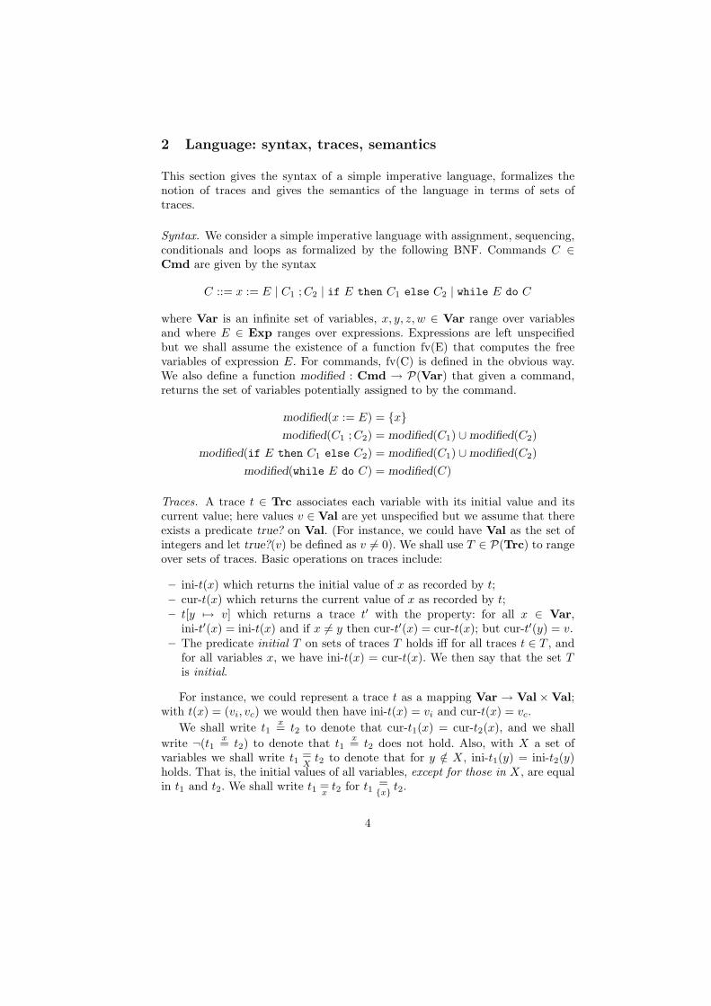
2 Language: syntax, traces, semantics

This section gives the syntax of a simple imperative language, formalizes thenotion of traces and gives the semantics of the language in terms of sets oftraces.

Syntax. We consider a simple imperative language with assignment, sequencing,conditionals and loops as formalized by the following BNF. Commands C ∈Cmd are given by the syntax

C ::= x := E | C1 ;C2 | if E then C1 else C2 | while E do C

where Var is an infinite set of variables, x, y, z, w ∈ Var range over variablesand where E ∈ Exp ranges over expressions. Expressions are left unspecifiedbut we shall assume the existence of a function fv(E) that computes the freevariables of expression E. For commands, fv(C) is defined in the obvious way.We also define a function modified : Cmd → P(Var) that given a command,returns the set of variables potentially assigned to by the command.

modified(x := E) = {x}modified(C1 ;C2) = modified(C1) ∪modified(C2)

modified(if E then C1 else C2) = modified(C1) ∪modified(C2)modified(while E do C) = modified(C)

Traces. A trace t ∈ Trc associates each variable with its initial value and itscurrent value; here values v ∈ Val are yet unspecified but we assume that thereexists a predicate true? on Val. (For instance, we could have Val as the set ofintegers and let true?(v) be defined as v 6= 0). We shall use T ∈ P(Trc) to rangeover sets of traces. Basic operations on traces include:

– ini-t(x) which returns the initial value of x as recorded by t;– cur-t(x) which returns the current value of x as recorded by t;– t[y 7→ v] which returns a trace t′ with the property: for all x ∈ Var,

ini-t′(x) = ini-t(x) and if x 6= y then cur-t′(x) = cur-t(x); but cur-t′(y) = v.– The predicate initial T on sets of traces T holds iff for all traces t ∈ T , and

for all variables x, we have ini-t(x) = cur-t(x). We then say that the set Tis initial.

For instance, we could represent a trace t as a mapping Var → Val ×Val;with t(x) = (vi, vc) we would then have ini-t(x) = vi and cur-t(x) = vc.

We shall write t1x= t2 to denote that cur-t1(x) = cur-t2(x), and we shall

write ¬(t1x= t2) to denote that t1

x= t2 does not hold. Also, with X a set ofvariables we shall write t1 =

Xt2 to denote that for y /∈ X, ini-t1(y) = ini-t2(y)

holds. That is, the initial values of all variables, except for those in X, are equalin t1 and t2. We shall write t1 =

xt2 for t1 =

{x} t2.

4

[[x := E]] = λT.{t′ | ∃t ∈ T : t′ = t[x 7→ [[E]](t)]}

[[C1 ; C2]] = λT.[[C2]]([[C1]](T ))

[[if E then C1 else C2]] = λT.[[C1]](E-true(T )) ∪ [[C2]](E-false(T ))

[[while E do C0]] = lfp(FC) where C = while E do C0 and

FC : (P(Trc) → P(Trc)) → (P(Trc) → P(Trc))

FC(f) = λT.f([[C0]](E-true(T ))) ∪ E-false(T )

Fig. 1. The Trace Semantics.

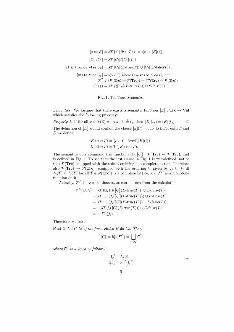
Semantics. We assume that there exists a semantic function [[E]] : Trc → Valwhich satisfies the following property:

Property 1. If for all x ∈ fv(E) we have t1x= t2, then [[E]](t1) = [[E]](t2).

The definition of [[E]] would contain the clause [[x]](t) = cur-t(x). For each T andE we define

E-true(T ) = {t ∈ T | true?([[E]](t))}E-false(T ) = T \ E-true(T ).

The semantics of a command has functionality [[C]] : P(Trc) → P(Trc), andis defined in Fig. 1. To see that the last clause in Fig. 1 is well-defined, noticethat P(Trc) equipped with the subset ordering is a complete lattice. Thereforealso P(Trc) → P(Trc) (equipped with the ordering v given by f1 v f2 ifff1(T ) ⊆ f2(T ) for all T ∈ P(Trc)) is a complete lattice, and FC is a monotonefunction on it.

Actually, FC is even continuous, as can be seen from the calculation

FC(tifi) = λT.(tifi)([[C]](E-true(T ))) ∪ E-false(T )= λT. ti (fi([[C]](E-true(T )))) ∪ E-false(T )= λT. ti (fi([[C]](E-true(T ))) ∪ E-false(T ))= tiλT.fi([[C]](E-true(T ))) ∪ E-false(T )= tiFC(fi)

Therefore, we have

Fact 1 Let C be of the form while E do C0. Then

[[C]] = lfp(FC) =⊔

i∈NfCi

where fCi is defined as follows:

fC0 = λT.∅

fCi+1 = FC(fC

i )

5

3 Independences

We are interested in a finite abstraction of a (possibly infinite) set of concretetraces. The abstract values are termed independences: an independence T# ∈Independ = P(Var×Var) is a set of pairs of the form [x# w], denoting thatthe current value of x is independent of the initial value of w. This is formalizedby the following definition of when an independence correctly describes a set oftraces. The intuition is that x is independent of w iff any two traces which havethe same initial values except on w must agree on the current value of x; in otherwords, the initial value of w does not influence the current value of x at all.

Definition 1. [x# w] |= T holds iff for all t1, t2 ∈ T : t1 =w

t2 implies t1x= t2.

T# |= T holds iff for all [x# w] ∈ T# it holds that [x# w] |= T .

Definition 2. The ordering T#1 � T#

2 holds iff T#2 ⊆ T#

1 .

This is motivated by the desire for a subtyping rule, stating that if T#1 � T#

2

then T#1 can be replaced by T#

2 (cf. Fact 3). Such a rule is sound provided T#2 is a

subset of T#1 and therefore obtainable from T#

1 by removing information. Clearly,Independ forms a complete lattice wrt. the ordering; let uiT

#i denote the

greatest lower bound (which is the set union). We have some expected properties:

Fact 2 If T# |= T and T1 ⊆ T then T# |= T1.

Fact 3 If T#1 |= T and T#

1 � T#2 then T#

2 |= T .

Fact 4 If for all i ∈ I it holds that T#i |= T , then ui∈IT

#i |= T .

To see the latter, note that if [x# w] belongs to uiT#i then it also belongs to

some T#i . Moreover, we can write a concretization function γ : Independ →

P(P(Trc)):γ(T#) = {T | T# |= T}

The following calculation shows that γ is completely multiplicative:

T ∈ γ(uiT#

i) ⇔ ∀[x# y] ∈ uiT#

i • [x# y] |= T

⇔ ∀i • ∀[x# y] ∈ T#i • [x# y] |= T

⇔ ∀i • T ∈ γ(T#i )

⇔ T ∈⋂i

γ(T#i )

Therefore [21] there exists a Galois connection between P(P(Trc)) and Independ,with γ the concretization function. Finally, we have the following fact about ini-tial sets of traces.

Fact 5 For all T , if initial T then [x# y] |= T for all x 6= y.

6

4 Static Checking of Independences

To statically check independences we define, in Fig. 2, a Hoare-like Logic wherejudgements are of the form G ` {T#

1 } C {T#2 }. The judgement is interpreted

as saying that if the independences in T#1 hold before execution of C then,

provided C terminates, the independences in T#2 will hold after execution of

C. The context G ∈ Context = P(Var) is a control dependence, denoting (asuperset of) the variables that at least one test surrounding C depends on. Forexample, in if x then y := 0 else z := 1, the static checking of y := 0 takesplace in the context that contains all variables that x is dependent on. This iscrucial, especially since x may depend on a high variable.

We now explain a few of the rules in Fig. 2. Checking an assignment, x := E,in context G, involves checking any [y # w] in the postcondition T#. There aretwo cases. If x 6= y, then [y # w] must also appear in the precondition T#

0 . Oth-erwise, if x = y then [x# w] appears in the postcondition provided all variablesreferenced in E are independent of w; moreover, w must not appear in G, asotherwise, x would be (control) dependent on w.

Checking a conditional, if E then C1 else C2, involves checking C1 and C2

in a context G0 that includes not only the “old” context G but also the variablesthat E depends on (as variables modified in C1 or C2 will be control dependenton such). Equivalently, if w is not in G0, then all free variables x in E must beindependent of w, that is, [x# w] must appear in the precondition T#

0 .Checking a while loop is similar to checking a conditional. The only difference

is that it requires guessing an “invariant” T# that is both the precondition andthe postcondition of the loop and its body.

In Section 6, when we define strongest postcondition, we will select G0 = G∪{w | ∃x ∈ fv(E) • [x# w] /∈ T#

0 } for the conditional and the while loop. Insteadof guessing the invariant, we will show how to compute it using fixpoints.

Example 1. We have the derivations

∅ ` {{[l # h], [h # l]}} l := h {{[h # l], [l # l]}} and∅ ` {{[h # l], [l # l]}} l := 0 {{[h # l], [l # l], [l # h]}}

and therefore also

∅ ` {{[l # h], [h # l]}} l := h ; l := 0 {{[h # l], [l # l], [l # h]}}

With the intuition that l stands for “low” or “public” and h stands for“high” or “sensitive”, the derivation asserts that if l is independent of h beforeexecution, then provided the program halts, l is independent of h after execution.By Definition 1, any two traces of the program with different initial values for h,agree on the current value for l. Thus the program is secure, although it containsan insecure sub-program.

Example 2. The reader may check that the following informally annotated pro-gram gives rise to a derivation in our logic. Initially, G is empty, and all variables

7

[Assign] G ` {T#0 } x := E {T#}

if ∀[y # w] ∈ T#•x 6= y ⇒ [y # w] ∈ T#

0

x = y ⇒ w /∈ G ∧ ∀z ∈ fv(E) • [z # w] ∈ T#0

[Seq]G ` {T#

0 } C1 {T#1 } G ` {T#

1 } C2 {T#2 }

G ` {T#0 } C1 ; C2 {T#

2 }

[If]G0 ` {T#

0 } C1 {T#} G0 ` {T#0 } C2 {T#}

G ` {T#0 } if E then C1 else C2 {T#}

if G ⊆ G0

and w /∈ G0 ⇒ ∀x ∈ fv(E) • [x # w] ∈ T#0

[While]G0 ` {T#} C {T#}

G ` {T#} while E do C {T#}if G ⊆ G0

and w /∈ G0 ⇒ ∀x ∈ fv(E) • [x # w] ∈ T#

[Sub]G1 ` {T#

1 } C {T#2 }

G0 ` {T#0 } C {T#

3 }if T#

0 � T#1 and T#

2 � T#3 and G0 ⊆ G1

Fig. 2. The Hoare Logic.

are pairwise independent; we write [x# y, z] to abbreviate [x# y], [x# z].

{[l # h, x], [h # l, x], [x# l, h]}x := h {[l # h, x], [h # l, x], [x# l, x]}if x > 0 (G is now {h})

then l := 7 {[l # x, l], [h # l, x], [x# l, x]}else x := 0 {[l # h, x], [h # l, x], [x# l, x]}

end of if {[l # x], [h # l, x], [x# l, x]}

A few remarks:

– in the preamble, only x is assigned, so the independences for l and h arecarried through, but [x# l, x] holds afterwards, as [h # l, x] holds beforehand;

– the free variable in the guard is independent of l and x but not of h, implyingthat h has to be in G.

In a judgement G ` {T#0 } C {T#}, suppose w ∈ G. This means that any

assignment in C is control dependent on w. Suppose now that y is independentof w in the postcondition T#. This implies that y cannot be assigned to in C— otherwise, it would be dependent on w. If y is not assigned to in C, then ymust be independent of w in the precondition too. These intuitions are collectedtogether in Lemma 1 below. Note that with y interpreted as “low” and w as“high”, the lemma essentially says that low variables may not be written tounder a high guard. Thus the lemma is the counterpart of the “no write down”rule that underlies information flow control; the term “*-property” [6] is alsoused. The value of low variables remains the same after execution of C.

8

Lemma 1 (Write Confinement).Assume that G ` {T#

0 } C {T#} and [y # w] ∈ T# and w ∈ G.Then y /∈ modified(C) and [y # w] ∈ T#

0 .

The proof is given in Appendix B.

5 Correctness

We are now in a position to prove the correctness of the Hoare logic with respectto the trace semantics.

Theorem 6. Assume that

G ` {T#0 } C {T#} where for all [x# y] ∈ T#

0 , it is the case that x 6= y.

Then, initial T implies T# |= [[C]](T ).

That is, if T is an initial set, then T# correctly describes the set of concretetraces obtained by executing command C on T .

The correctness theorem can be seen as the noninterference theorem for infor-mation flow. Indeed, with l and h interpreted as “low” and “high” respectively,suppose [l # h] appears in T#. Then any two traces in [[C]](T ) (the set of tracesresulting from the execution of command C from initial set T ) that have initialvalues that differ only on h, must agree on the current value of l.

Note that the correctness result deals with “terminating” traces only. Forexample, with P = while h 6= 0 do h := 7 and T# = {[l # h], [h # l]} we havethe judgement ∅ ` {T#} P {T#} (since {h} ` {T#} h := 7 {T#}) showing thatP is deemed secure by our logic, yet an observer able to observe non-terminationcan detect whether h was initially 0 or not.

To prove Theorem 6, we claim the following, more general, lemma. Thenthe theorem follows by the lemma using Fact 5. The proof can be found inAppendix B.

Lemma 2. If G ` {T#0 } C {T#} and T#

0 |= T then also T# |= [[C]](T ).

6 Computing Independences

In Fig. 3 we define a function

sp : Context×Cmd× Independ → Independ

with the intuition (formalized below) that given a control dependence G, a com-mand C and a precondition T#, sp(G, C, T#) computes a postcondition T#

1 suchthat G ` {T#} C {T#

1 } holds, and T#1 is the “largest” set (wrt. the subset order-

ing) that makes the judgement hold. Thus we compute the “strongest provable

9

postcondition”, which might differ3 from the strongest semantic postcondition,that is, the largest set T#

1 such that for all T , if T# |= T then T#1 |= [[C]](T ).

We now explain two of the cases in Fig. 3. In an assignment, x := E, thepostcondition carries over all independences [y # w] in the precondition if y 6= x;these independences are unaffected by the assignment to x. Suppose that w doesnot occur in context G. Then x is not control dependent on w. Moreover, ifall variables referenced in E are independent of w, then [x# w] will be in thepostcondition of the assignment.

The case for while is best explained by means of an example.

Example 3. Consider the program

C = while y do l := x ;x := y ; y := h.

Let T#0 . . . T#

8 be given by the following table. For example, the entry in thecolumn for T#

4 and in the row for x shows that [x# h] ∈ T#4 and [x# l] ∈ T#

4 .

T#0 T#

1 T#2 T#

3 T#4 T#

5 T#6 T#

7 T#8

h # {l, x, y} {l, x, y} {l, x, y} {l, x, y} {l, x, y} {l, x, y} {l, x, y} {l, x, y} {l, x, y}l # {h, x, y} {h, l} {h, l} {h, l} {h} {l} {l} ∅ {l}x # {h, l, y} {h, l, y} {h, l, x} {h, l, x} {h, l} {h, l} {l, x} {l} {l}y # {h, l, x} {h, l, x} {h, l, x} {l, x} {l, x} {l, x} {l, x} {l, x} {l, x}

Our goal is to compute sp(∅, C, T#0 ) and doing so involves the fixed point com-

putation sketched below.

Iterationfirst second third

while y do T#0 T#

4 = T#3 ∩ T#

0 T#7 = T#

6 ∩ T#0

G0 : {y} {h, y} {h, y}l := x T#

1 T#5 T#

8

x := y T#2 T#

6 T#6

y := h T#3 T#

6 T#6

For example, the entry T#6 in the column marked “second” and in the second

row from the bottom, denotes that sp({h, y}, x := y, T#5 ) = T#

6 .Note that after the first iteration, [l # h] is still present; it takes a second

iteration to filter it out and thus detect insecurity. The third iteration affirms

that T#7 is indeed a fixed point (of the functional HT#

0 ,∅C defined in Fig. 3).

Theorem 7 states the correctness of the function sp, that it indeed computesa postcondition. Then, Theorem 8 states that the postcondition computed by spis the strongest postcondition. We shall rely on the following property:

3 For example, let C = l := h− h and T# = {[l # h]}. Then [l # h] is in the strongestsemantic postcondition, since for all T and all t ∈ [[C]](T ) we have cur-t(l) = 0 andtherefore [l # h] |= [[C]]T , but not in the strongest provable postcondition.

10

sp(G, x := E, T#) =

{[y # w] | y 6= x ∧ [y # w] ∈ T#} ∪ {[x # w] | w /∈ G ∧ ∀y ∈ fv(E) • [y # w] ∈ T#}

sp(G, C1 ; C2, T#) = sp(G, C2, sp(G, C1, T

#))

sp(G, if E then C1 else C2, T#) =

let G0 = G ∪ {w | ∃x ∈ fv(E) • [x # w] /∈ T#}T#

1 = sp(G0, C1, T#)

T#2 = sp(G0, C2, T

#)

in T#1 ∩ T#

2

sp(G, while E do C0, T#) =

let HT#,GC : Independ → Independ be given by (C = while E do C0)

HT#,GC (T#

0 ) =

let G0 = G ∪ {w | ∃x ∈ fv(E) • [x # w] /∈ T#0 }

in sp(G0, C0, T#0 ) ∩ T#

in lfp(HT#,GC )

Fig. 3. Strongest Postcondition.

Lemma 3 (Monotonicity). For all C, the following holds (for all G,G1,T#,T#1 ):

1. sp(G, C, T#) is well-defined;2. if G ⊆ G1 then sp(G, C, T#) � sp(G1, C, T#);3. if T# � T#

1 then sp(G, C, T#) � sp(G, C, T#1 ).

The proof is given in Appendix C.

Theorem 7. For all C, G, T#, it holds that G ` {T#} C {sp(G, C, T#)}.

The proof is given in Appendix C.

Theorem 8. For all judgements G ` {T#1 } C {T#}, sp(G, C, T#

1 ) � T#.

The proof is given in Appendix C.The following result is useful for the developments in Sections 7 and 9:

Lemma 4. Given y, C with y /∈ modified(C). Then for all T#, G, w:

[y # w] ∈ T# implies [y # w] ∈ sp(G, C, T#)

The proof is given in Appendix D.

7 Modularity and the Frame Rule

Define lhs(T#) = {y | [y # w] ∈ T#}. Then we have

Theorem 9 (Frame rule (I)). Let T#0 and C be given. Then for all T#, G:

11

1. If lhs(T#0 )∩modified(C) = ∅ then sp(G, C, T# ∪ T#

0 ) ⊇ sp(G, C, T#)∪ T#0 .

2. If lhs(T#0 ) ∩ fv(C) = ∅ then sp(G, C, T# ∪ T#

0 ) = sp(G, C, T#) ∪ T#0 .

Note that the weaker premise in 1 does not imply the stronger consequence in2, since (with [z # w] playing the role of T#

0 )

sp(∅, x := y + z, {[y # w]} ∪ {[z # w]}) = {[y # w], [z # w], [x# w]}sp(∅, x := y + z, {[y # w]}) ∪ {[z # w]} = {[y # w], [z # w]}.

In separation logic [18, 26], the frame rule is motivated by the desire for localreasoning: if C1 and C2 modify disjoint regions of a heap, reasoning about C1

can be performed independently of the reasoning about C2. In our setting, aconsequence of the frame rule is that when analyzing a command C occurring ina larger context, the relevant independences are the ones whose left hand sidesoccur in C.

Theorem 9 is proved by observing that part (1) follows from Lemmas 4 and3; then part (2) follows using the following result which is proved in Appendix D.

Lemma 5. Let T#0 and C be given, with lhs(T#

0 ) ∩ fv(C) = ∅. Then for all T#

and G, sp(G, C, T# ∪ T#0 ) ⊆ sp(G, C, T#) ∪ T#

0 .

As a consequence of Theorem 9 we get the following result:

Corollary 1 (Frame rule (II)). Assume that G ` {T#1 } C {T#

2 } and thatlhs(T#

0 ) ∩modified(C) = ∅. Then G ` {T#1 ∪ T#

0 } C {T#2 ∪ T#

0 }.

Proof. Using Theorems 9 and 8 we get

sp(G, C, T#1 ∪ T#

0 ) ⊇ sp(G, C, T#1 ) ∪ T#

0 ⊇ T#2 ∪ T#

0 .

Since by Theorem 7 we have G ` {T#1 ∪ T#

0 } C {sp(G, C, T#1 ∪ T#

0 )}, the resultfollows by [Sub].

Example 4. Assume that

G ` {T#1 } C1 {T#

3 } and G ` {T#2 } C2 {T#

4 }.

Further assume that lhs(T#2 )∩modified(C1) = ∅ and that lhs(T#

3 )∩modified(C2) =∅. Then Corollary 1 yields

G ` {T#1 ∪ T#

2 } C1 {T#3 ∪ T#

2 } and G ` {T#3 ∪ T#

2 } C2 {T#3 ∪ T#

4 }

and therefore G ` {T#1 ∪ T#

2 } C1 ;C2 {T#3 ∪ T#

4 }.

A traditional view of modularity in the security literature is the “hook-up prop-erty” [20]: if two programs are secure then their composition is secure as well.Our logic satisfies the hook-up property for sequential composition; in our con-text, a secure program is one which has [l # h] as an invariant (if [l # h] is in theprecondition, it is also in the strongest postcondition). With this interpretation,Sabelfeld and Sands’s hook-up theorem holds [29, Theorem 5].

12

8 The Smith-Volpano Security Type System

In the Smith-Volpano type system [30], variables are labelled by security types;for example, x : (T, κ) means that x has type T and security level κ. The securitytyping rules are given in Fig. 5 in Appendix E. To handle implicit flows due toconditionals, the technical development requires commands to be typed (comκ)with the intention that all variables assigned to in such commands have level atleast κ. The judgement Γ ` C : (com κ) says that in the security type context Γ ,that binds free variables in C to security types, command C has type (com κ).

We now show a conservative extension: if a command is well-typed in theSmith-Volpano system, then for any two traces, the current values of low vari-ables are independent of the initial values of high variables. For simplicity, weconsider a command with only two variables, h with level H and l with level L.

Theorem 10. Assume that C can be given a security type wrt. the environmenth : ( ,H), l : ( , L). Then for all T#, if [l # h] ∈ T# then [l # h] ∈ sp(∅, C, T#).

The upshot of the theorem is that a well-typed program has [l # h] as invari-ant : if [l # h] appears in the precondition, then it also appears in the strongestpostcondition.

The theorem is a straightforward consequence of the following lemma whichfacilitates a proof by induction. For L commands, the assumption h 6∈ G in thelemma says that L commands cannot be control dependent on H guards. Aproof appears in Appendix E.

Lemma 6. 1. Suppose h : ( ,H), l : ( , L) ` C : (com H). Then for all G, T#,if [l # h] ∈ T# then [l # h] ∈ sp(G, C, T#).

2. Suppose h : ( ,H), l : ( , L) ` C : (com L). Then for all G, T#, if [l # h] ∈T# and h 6∈ G then [l # h] ∈ sp(G, C, T#).

9 Counter-example Generation

Assume that a program C cannot be deemed secure by our logic, that is, [l # h] /∈sp(∅, C, T#) (where T# ⊇ {[l # h]}). Then we might expect that we can finda “witness”: two different initial values of h that produce two different finalvalues of l. However, in Section 9.1 we shall see three examples of false positives:programs which, while deemed insecure by our logic, do not immediately satisfythat property. Ideally, we would like to strengthen our analysis so as to ruleout such false positives; this does not seem immediately feasible and instead, inorder to arrive at a suitable result, we shall modify our semantics so the falsepositives become genuine positives.

9.1 Issues to be Addressed

First, a program where writing a high expression to a low variable does notreveal anything about the high variable:

13

l := h− h. (1)

To deal with that, we assume that expressions are unevaluated (kept as symbolictrees); the formal requirement will be expressed as Property 2.

Next, a program where writing to a low variable under high guard does notimmediately enable an observer to determine the value of the high variable.

if h then l := 7 else l := 7 (2)

To deal with that, we tag each assignment statement so that an observer candetect which branch is taken.

Finally, a program where there cannot be two different final values of l:

while h do l := 7 (3)

There seems to be no simple way to fix this, except to rule out loops, thus ineffect considering only programs with a fixed bound on run-time (since for such,a loop can be unfolded repeatedly and eventually replaced by a sequence ofconditionals; this is how we handle loops with low guard). Remember (cf. thediscussion in Section 5) that a program deemed secure by our logic may not bereally secure if non-termination can be observed; similarly a program deemedinsecure may not be really insecure if non-termination cannot be observed.

Even with the above modifications, the existence of a witness is not amenableto a compositional proof. For example, consider the program

x := E1(h) ; l := E2(x) (4)

where E1 and E2 are some expressions. Inductively, on the assignment to l, wecan find two different values for x, v1 and v2, such that the resulting values ofl are different. But we then need an extremely strong property concerning theassignment to x: that there exists two different values of h such that evaluatingE1(h) wrt. these values produces v1, respectively v2.

Instead, we shall settle for a result which says that all pairs of different initialvalues for h are witnesses, in that the resulting values of l are different. Of course,we need to introduce some extra assumptions to establish this stronger property.For example, consider the following program, where two different values of h,say 3 and 4, may cause the same branch to be taken:

if h = 0 then l := 17 else l := 7 (5)

To deal with that, our result must say that for every two values of h there existsan interpretation of true? such that wrt. that interpretation, different values of lresult. In the above, we might stipulate that true?(3 = 0) but not true?(4 = 0).It turns out to be convenient to let that interpretation depend on the guard inquestion; hence we shall also tag guards so as to distinguish between differentoccurrences of the same guard.

14

9.2 Revised Syntax

We shall now formalize the changes suggested in the previous section. First, weassume the existence of tags τ ∈ Tag, and functions

tg : Tag×Val → Val, get-tg : Val → Tag, un-tg : Val → Val

such that get-tg(tgτ (v)) = τ and un-tg(tgτ (v)) = v.Commands C are now given by the syntax

C ::= τ : x := E | C1 ;C2 | if τ : E then C1 else C2

where we have introduced assignment tags and guard tags. We write tg-t(x) forget-tg(cur-t(x)), write τ ∈ C if τ occurs syntactically in C, and write t ∆ C iffor all x ∈ Var, tg-t(x) /∈ C.

In the following, we shall assume that tags are unique, that is, no tag τ occurstwice in a program C.

9.3 Revised Semantics

As mentioned in Sect. 9.1, for the purposes of this section we shall rely on thefollowing

Property 2. If there exists z ∈ fv(E) with ¬(t1z= t2), then [[E]](t1) 6= [[E]](t2).

Concerning how to modify the semantics of commands, first observe that withthe definition in Fig. 1, it holds for programs without loops that [[C]] appliedto a singleton set {t} returns a singleton set (this follows from a simple struc-tural induction, simultaneously proving that [[C]](∅) = ∅). This motivates thatwe should now define the semantics as a function from Trc to Trc (rather thanbetween the powersets), but as mentioned in Sect. 9.1 we shall also need in-terpretation functions where an interpretation function I ∈ Intp is a partiallydefined predicate on values. We say that I covers C if I(v) is defined exactlywhen there exists a guard tag τ ∈ C such that v = tgτ (v0) for some v0. Notethat if C1 and C2 are disjoint parts of a program, and there exists I1 coveringC1 and I2 covering C2, then the union of I1 and I2 will be well-defined (due toour assumption about unique tagging).

The semantics of a command thus has functionality Intp → Trc → Trc andis defined as follows:

[[τ : x := E]]I = λt.t[x 7→ tgτ ([[E]](t))][[C1 ;C2]]I = λt.[[C2]]I([[C1]]I(t))

[[if τ : E then C1 else C2]]I = λt.cond(I(tgτ ([[E]](t))), [[C1]]I(t), [[C2]]I(t)).

Clearly, if [[C]]I(t) = t′ then also [[C]]I1(t) = t′ for any I1 that extends I.

15

9.4 Counter-example Theorem

We can now state our result concerning counter-examples; as discussed in Sect. 9.1it seems to be the best we can hope for.

Theorem 11. Assume that sp(∅, C, T#) = T#1 , with [x# h] ∈ T# for x 6= h

and with [l # h] /∈ T#1 . Further assume that ¬(t1

h= t2), with t1 ∆ C and t2 ∆ C.Then there exists I covering C such that ¬([[C]]I(t1)

l= [[C]]I(t2)).

This theorem is a straightforward consequence of Lemma 7, stated below.

Definition 3. We say that C reveals y using z if for all t1, t2 with t1 ∆ C andt2 ∆ C and ¬(t1

z= t2) there exists an interpretation function I covering C suchthat ¬([[C]]I(t1)

y= [[C]]I(t2)).

Lemma 7. Assume that with h /∈ G we have sp(G, C, T#) = T#1 , and assume

that [y # h] /∈ T#1 . Then there exists z such that [z # h] /∈ T#, and such that C

reveals y using z.

The proof is given in Appendix F.

Example 5. We consider an adaptation of the password checking example from[7], with the while loop unfolded twice.

if τ1 : p = g1 then τ2 : f := 1else if τ3 : p = g2

then τ4 : f := 1else τ5 : f := 2

By Theorem 11 there exists an interpretation function, I, such that for twodistinct values of p, namely, p1 and p2, f assumes different values. The I providedby the proof of the theorem will satisfy I(tgτ1

(p1 = g1)) = true but I(tgτ1(p2 =

g1)) = false. Then p1 will result in a value of f which is tagged with τ2, and p2

will result in another value of f which is tagged with either τ4 or τ5 (dependingon the value of I(tgτ3

(p2 = g2))). Hence the particular branch taken for thecomputation is revealed.

10 Discussion

Perspective. This paper specifies an information flow analysis for confidentialityusing a Hoare-like logic and considers an application of the logic to explaininginsecurity in simple imperative programs. Program traces, potentially infinitelymany, are abstracted by finite sets of variable independences. These variableindependences can be statically computed using strongest postconditions, andcan be statically checked against the logic.

Giacobazzi and Mastroeni [13] consider attackers as abstract interpretationsand generalize the notion of noninterference by parameterizing it wrt. what anattacker can analyze about the input/output information flow. For instance,assume an attacker can only analyze the parity (odd/even) of values. Then

16

while h do l := l + 2 ;h := h− 1

is secure, although it contains an update of a low variable under a high guard.We might try to model this approach in our framework by parameterizing Defi-nition 1 wrt. parity, but it is not clear how to alter the proof rules accordingly.Instead, we envision our logic to be put on top of abstract interpretations. Inthe parity example, the above program would be abstracted to

while h do h := h− 1

which our logic already deems secure.

Related work. Perhaps the most closely related work is the one of Clark, Han-kin, and Hunt [7], who consider a language similar to ours and then extend it toIdealized Algol, requiring distinguishing between identifiers and locations. Theanalysis for Idealized Algol is split in two stages: the first stage does a control-flow analysis, specified using a flow logic [21]. The second stage specifies what isan acceptable information flow analysis with respect to the control-flow analysis.The precision of the control-flow analysis influences the precision of the infor-mation flow analysis. Flow logics usually do not come with a frame rule so it isunclear what modularity properties their analysis satisfies. For each statementS in the program, they compute the set of dependences introduced by S; a pair(x, y) is in that set if different values for y prior to execution of S may result indifferent values for x after execution of S. For a complete program, they thus,as expected, compute essentially the same information as we do, but the infor-mation computed locally is different from ours: we estimate if different initialvalues of y, i.e., values of y prior to execution of the whole program, may resultin different values for x after execution of S. Unlike our approach, their analysisis termination-sensitive.

To make our logic termination-sentitive4, we could (analogous in spirit to[7]) define [⊥ # w] to mean that if two tuples of initial values are equal exceptfor on w, then either both tuples give rise to terminating computations, or bothtuples give rise to infinite computations. For instance, if

` {T#0 } while x > 7 do x := x + 1 {T#}

and [x# h] does not belong to T#0 then [⊥ # h] should not belong to T# (neither

of any subsequent assertion), since different values of h may result in differentvalues of x and hence of different termination properties. To prove semanticcorrectness for the revised logic we would need to also revise our semantics,since currently it does not facilitate reasoning about infinite computations.

Joshi and Leino [19] provide an elegant semantic characterization of non-interference that allows handling both termination-sensitive and termination-insensitive noninterference. Their notion of security for a command C is equa-tionally characterized by C ;HH = HH ;C ;HH, where HH means that an4 For an analysis protecting against timing leaks and hence as a special case against

attackers observing termination behavior, see [2].

17

arbitrary value is assigned to a high variable. They show how to express theirnotion of security in Dijkstra’s weakest precondition calculus. Although they donot consider synthesizing loop invariants, this can certainly be done via a fixpointcomputation with weakest preconditions. However, their work is not concernedwith computing dependences, nor do they consider generating counterexamples.

Darvas, Hahnle and Sands [11] use dynamic logic to express secure informa-tion flow in JavaCard. They discuss several ways that noninterference can beexpressed in a program logic, one of which is as follows: consider a program withvariables l and h. Consider another copy of the program with l, h relabeled tofresh variables l′, h′ respectively. Then, noninterference holds in the followingsituation: running the original program and the copy sequentially such that theinitial state satisfies l = l′ should yield a final state satisfying l = l′. Like us,they are interested in showing insecurity by exhibiting distinct initial values forhigh variables that give distinct current values of low variables; unlike us, theylook at actual runtime values. To achieve this accuracy, they need the power ofa general purpose theorem prover, which is also helpful in that they can expressdeclassification, as well as treat exceptions (which most approaches based onstatic analysis cannot easily be extended to deal with).

Barthe, D’Argenio and Rezk [5] use the same idea of self-composition (i.e.,composing a program with a copy of itself) as Darvas et alii and investigate“abstract” noninterference [13] for several languages. By parameterizing non-interference with a property, they are able to handle more general informationflow policies, including a form of declassification known as delimited informationrelease [27]. They show how self-composition can be formulated in logics describ-ing these languages, namely, Hoare logic, separation logic, linear temporal logic,etc. They also discuss how to use their results for model checking programswith finite state spaces to check satisfaction of their generalized definition ofnoninterference.

The first work that used a Hoare-style semantics to reason about informationflow was by Andrews and Reitman [3]. Their assertions keep track of the securitylevel of variables, and are able to deal even with parallel programs. However, noformal correctness result is stated.

Conclusion. Beyond the work reported here, much remains to be done. Thispaper was inspired in part by presentations by Roberto Giacobazzi and ReinerHahnle at the Dagstuhl Seminar on Language-based Security in October 2003.The reported work is only the first step in our goal to formulate more generaldefinitions of noninterference in terms of program (in)dependence, such that thedefinitions support modular reasoning. One direction to consider is to repeatthe work in this paper for a richer language, with methods, pointers, objectsand dynamic memory allocation; an obvious goal here is interprocedural reason-ing about variable independences perhaps using a higher-order version of theframe rule [23]. Hahnle’s Dagstuhl presentation inspired us to look at explain-ing insecurity by showing counterexamples. We plan to experiment with modelcheckers supporting linear arithmetic, for example BLAST [16], to (i) establishindependences that our logic cannot find (cf. the false positives from Sect. 9); (ii)

18

provide “genuine” counterexamples that are counterexamples wrt. the originalsemantics.

Acknowledgements. We would like to thank Reiner Hahnle, Peter O’Hearn,Tamara Rezk, David Sands, and Hongseok Yang, as well as the participantsof the Open Software Quality meeting in Santa Cruz, May 2004, and the anony-mous reviewers of SAS 2004, for useful comments on a draft of this report.

References

1. Martın Abadi, Anindya Banerjee, Nevin Heintze, and Jon G. Riecke. A core calcu-lus of dependency. In ACM Symposium on Principles of Programming Languages(POPL), pages 147–160, 1999.

2. Johan Agat. Transforming out timing leaks. In POPL’00, Boston, Massachusetts,pages 40–53. ACM Press, 2000.

3. G. R. Andrews and R. P. Reitman. An axiomatic approach to information flow inprograms. ACM Transactions on Programming Languages and Systems, 2(1):56–75, January 1980.

4. Anindya Banerjee and David A. Naumann. Secure information flow and pointerconfinement in a Java-like language. In IEEE Computer Security FoundationsWorkshop (CSFW), pages 253–270. IEEE Computer Society Press, 2002.

5. Gilles Barthe, Pedro R. D’Argenio, and Tamara Rezk. Secure information flowby self-composition. In IEEE Computer Security Foundations Workshop (CSFW),2004. To appear.

6. D.E. Bell and L.J. LaPadula. Secure computer systems: Mathematical foundations.Technical Report MTR-2547, MITRE Corp., 1973.

7. David Clark, Chris Hankin, and Sebastian Hunt. Information flow for Algol-likelanguages. Computer Languages, 28(1):3–28, 2002.

8. Ellis S. Cohen. Information transmission in sequential programs. In Richard A.DeMillo, David P. Dobkin, Anita K. Jones, and Richard J. Lipton, editors, Foun-dations of Secure Computation, pages 297–335. Academic Press, 1978.

9. Patrick Cousot and Radhia Cousot. Abstract interpretation: a unified lattice modelfor static analysis of programs by construction or approximation of fixpoints. InACM Symposium on Principles of Programming Languages (POPL), pages 238–252. ACM Press, New York, NY, 1977.

10. Patrick Cousot and Radhia Cousot. Automatic synthesis of optimal invariantassertions: mathematical foundations. In Proceedings of the ACM Symposium onArtificial Intelligence and Programming Languages, SIGPLAN Notices, volume 12,pages 1–12. ACM Press, August 1977.

11. Adam Darvas, Reiner Hahnle, and Dave Sands. A theorem proving approachto analysis of secure information flow. Technical Report 2004-01, Department ofComputing Science, Chalmers University of Technology and Goteborg University,2004. A fuller version of a paper appearing in Workshop on Issues in the Theoryof Security, 2003.

12. Dorothy Denning and Peter Denning. Certification of programs for secure infor-mation flow. Communications of the ACM, 20(7):504–513, 1977.

13. Roberto Giacobazzi and Isabella Mastroeni. Abstract non-interference: Parame-terizing non-interference by abstract interpretation. In ACM Symposium on Prin-ciples of Programming Languages (POPL), pages 186–197, 2004.

19

14. J. Goguen and J. Meseguer. Security policies and security models. In Proc. IEEESymp. on Security and Privacy, pages 11–20, 1982.

15. Nevin Heintze and Jon G. Riecke. The SLam calculus: programming with se-crecy and integrity. In ACM Symposium on Principles of Programming Languages(POPL), pages 365–377, 1998.

16. Thomas A. Henzinger, Ranjit Jhala, Rupak Majumdar, and Gregoire Sutre. Soft-ware verification with Blast. In Tenth International Workshop on Model Checkingof Software (SPIN), volume 2648 of Lecture Notes in Computer Science, pages235–239. Springer-Verlag, 2003.

17. Sebastian Hunt and David Sands. Binding time analysis: A new PERspective.In Partial Evaluation and Semantics-Based Program Manipulation (PEPM ’91),volume 26 (9) of Sigplan Notices, pages 154–165, 1991.

18. Samin Ishtiaq and Peter W. O’Hearn. BI as an assertion language for mutabledata structures. In ACM Symposium on Principles of Programming Languages(POPL), pages 14–26, 2001.

19. Rajeev Joshi and K. Rustan M. Leino. A semantic approach to secure informationflow. Science of Computer Programming, 37:113–138, 2000.

20. Daryl McCullough. Specifications for multi-level security and a hook-up. In IEEESymposium on Security and Privacy, April 27-29, 1987, pages 161–166, 1987.

21. Flemming Nielson, Hanne Riis Nielson, and Chris Hankin. Prin-ciples of Program Analysis. Springer-Verlag, 1999. Web page atwww.imm.dtu.dk/~riis/PPA/ppa.html.

22. Peter O’Hearn, John Reynolds, and Hongseok Yang. Local reasoning about pro-grams that alter data structures. In Computer Science Logic, volume 2142 ofLNCS, pages 1–19. Springer, 2001.

23. Peter O’Hearn, Hongseok Yang, and John Reynolds. Separation and informationhiding. In ACM Symposium on Principles of Programming Languages (POPL),pages 268–280, 2004.

24. Peter Ørbæk and Jens Palsberg. Trust in the λ-calculus. Journal of FunctionalProgramming, 7(6):557–591, November 1997.

25. Francois Pottier and Vincent Simonet. Information flow inference for ML. ACMTransactions on Programming Languages and Systems, 25(1):117–158, January2003.

26. John C. Reynolds. Separation logic: a logic for shared mutable data structures.In IEEE Symposium on Logic in Computer Science (LICS), pages 55–74. IEEEComputer Society Press, 2002.

27. Andrei Sabelfeld and Andrew Myers. A model for delimited information release. InProceedings of the International Symposium on Software Security (ISSS’03), 2004.To appear.

28. Andrei Sabelfeld and Andrew C. Myers. Language-based information-flow security.IEEE J. Selected Areas in Communications, 21(1):5–19, January 2003.

29. Andrei Sabelfeld and David Sands. A Per model of secure information flow insequential programs. Higher-order and Symbolic Computation, 14(1):59–91, 2001.

30. Dennis Volpano and Geoffrey Smith. A type-based approach to program secu-rity. In Proceedings of TAPSOFT’97, number 1214 in Lecture Notes in ComputerScience, pages 607–621. Springer-Verlag, 1997.

A Weakest Precondition

In Fig. 4 we shall define a function

20

wp(x := E, T#) =

let T#0 = {[z # w] ∈ T# | x 6= z}∪ {[y # w] | y ∈ fv(E) ∧ [x # w] ∈ T#}

G = {w | [x # w] /∈ T#}in (T#

0 , G)

wp(C1 ; C2, T#) =

let (T#2 , G2) = wp(C2, T

#)

(T#1 , G1) = wp(C1, T

#2 )

in (T#1 , G1 ∩G2)

wp(if E then C1 else C2, T#) =

let (T#1 , G1) = wp(C1, T

#)

(T#2 , G2) = wp(C2, T

#)G0 = G1 ∩G2

T#0 = T#

1 ∪ T#2 ∪ {[y # w] | y ∈ fv(E) ∧ w /∈ G0}

in (T#0 , G0)

wp(while E do C0, T#) =

let GT#

C : Independ → Independ be given by (C = while E do C0)

GT#

C (T#0 ) =

let (T#1 , G1) = wp(C0, T

#0 )

in T#1 ∪ T# ∪ {[y # w] | y ∈ fv(E) ∧ w /∈ G1}

T#0 = gfp(GT#

C )

in (T#0 , wpG(C0, T

#0 ))

Fig. 4. Weakest Precondition.

wp : Cmd× Independ → Independ×Context

with the intuition that if wp(C, T#) = (T#0 , G0) then (T#

0 , G0) satisfies G0 `{T#

0 } C {T#} (Theorem 12), and is the “largest” pair doing so (Theorem 13).A piece of notation: if wp(C, T#) = (T#

0 , G0) then we write wpT(C, T#) = T#0

and wpG(C, T#) = G0.

Lemma 8. For all C, wp(C, T#) is well-defined for all T#. Moreover, if T# �T#

1 then wpT(C, T#) � wpT(C, T#1 ) and wpG(C, T#) ⊆ wpG(C, T#

1 ).

Proof. Induction in C, where the only non-trivial case is where C is of the formwhile E do C0.

Using the induction hypothesis on C0, we infer that for all T# it holds thatGT#

C is a monotone function on the complete lattice Independ. Hence gfp(GT#

C ),and thus wp(C, T#), is indeed well-defined.

Next assume that T# � T#1 . Then clearly GT#

C � GT#1

C (by the pointwise

ordering) and therefore gfp(GT#

C ) � gfp(GT#1

C ) which amounts to the desired

21

relation wpT(C, T#) � wpT(C, T#1 ). Applying the induction hypothesis on C0

then shows that wpG(C0,wpT(C, T#)) ⊆ wpG(C0,wpT(C, T#1 )) which amounts

to the desired relation wpG(C, T#) ⊆ wpG(C, T#1 ).

Theorem 12. If wp(C, T#) = (T#1 , G) then G ` {T#

1 } C {T#}.

Proof. Structural induction in C; we perform a case analysis.

C = x := E. Let (T#1 , G) = wp(C, T#), and assume [z # w] ∈ T#. There are

two cases:

– if x 6= z then [z # w] ∈ T#1 .

– if x = z then w /∈ G, and for all y ∈ fv(E) : [y # w] ∈ T#1 .

This establishes G ` {T#1 } C {T#}.

C = C1 ;C2. Assume that wp(C1 ;C2, T#) = (T#

1 , G1∩G2) because (T#2 , G2) =

wp(C2, T#) and (T#

1 , G1) = wp(C1, T#2 ). Inductively, we have

G1 ` {T#1 } C1 {T#

2 } and G2 ` {T#2 } C2 {T#}.

By [Sub], this implies

G1 ∩G2 ` {T#1 } C1 {T#

2 } and G1 ∩G2 ` {T#2 } C2 {T#}

from which we infer the desired relation

G1 ∩G2 ` {T#1 } C1 ;C2 {T#}.

C = if E then C1 else C2. Assume that wp(if E then C1 else C2, T#) =

(T#0 , G0) because (T#

1 , G1) = wp(C1, T#) and (T#

2 , G2) = wp(C2, T#) and

G0 = G1 ∩G2 and

T#0 = T#

1 ∪ T#2 ∪ {[y # w] | y ∈ fv(E) ∧ w /∈ G0}.

Inductively, we have

G1 ` {T#1 } C1 {T#} and G2 ` {T#

2 } C2 {T#}.

By [Sub], this implies

G0 ` {T#0 } C1 {T#} and G0 ` {T#

0 } C2 {T#}.

Since w /∈ G0 and y ∈ fv(E) implies [y # w] ∈ T#0 , this proves the desired relation

G0 ` {T#0 } if E then C1 else C2 {T#}.

C = while E do C0. Assume that wp(C, T#) = (T#0 , G0) because

T#0 = gfp(GT#

C ) and G0 = wpG(C0, T#0 ).

22

Since T#0 = GT#

C (T#0 ), we from the definition of GT#

C infer that

T#1 ⊆ T#

0 and T# ⊆ T#0 (1)

y ∈ fv(E) and w /∈ G1 implies [y # w] ∈ T#0 (2)

where (T#1 , G1) = wp(C0, T

#0 ). Thus G1 = G0. Inductively,

G0 ` {T#1 } C0 {T#

0 }

which by [Sub], using (1), implies G0 ` {T#0 } C0 {T#

0 }. Since (2) holds, we canapply [While] to get

G0 ` {T#0 } C {T#

0 }

and by one more application of [Sub], still using (1), we get the desired relationG0 ` {T#

0 } C {T#}.

Theorem 13. Assume that G ` {T#1 } C {T#}. Then, with (T#

0 , G0) = wp(C, T#),it holds that T#

1 � T#0 and G ⊆ G0.

Proof. We perform induction in the derivation of G ` {T#1 } C {T#}, and do a

case analysis on the last rule applied:

[Sub]. Assume that

G ` {T#1 } C {T#}

because with G ⊆ G1 and T#1 � T#

2 and T#3 � T# we have

G1 ` {T#2 } C {T#

3 }.

Inductively, with (T#4 , G4) = wp(C, T#

3 ), it holds that

T#2 � T#

4 and G1 ⊆ G4.

Let (T#0 , G0) = wp(C, T#). By Lemma 8 we infer that

T#4 � T#

0 and G4 ⊆ G0

which implies the desired relations T#1 � T#

0 and G ⊆ G0.

[Assign], with C = x := E. Assume that G ` {T#1 } C {T#}, and let (T#

0 , G0) =wp(C, T#). We have two proof obligations:

– given [y # w] ∈ T#0 , we must show [y # w] ∈ T#

1 . Note that [y # w] can bein T#

0 for two reasons:• y 6= x and [y # w] ∈ T#. From the side condition for [Assign] we see that

then also [y # w] ∈ T#1 .

• y ∈ fv(E) and [x# w] ∈ T#. From the side condition for [Assign] weagain see that [y # w] ∈ T#

1 .

23

– given w ∈ G, we must prove w ∈ G0. But from w ∈ G we infer (from theside condition for [Assign]) that [x# w] /∈ T#, implying w ∈ G0.

[Seq], with C = C1 ;C2. Assume that G ` {T#1 } C {T#} because

G ` {T#1 } C1 {T#

2 } and that G ` {T#2 } C2 {T#}.

By applying the induction hypothesis to these judgements, we get

G ⊆ G3 and T#1 � T#

3

G ⊆ G2 and T#2 � T#

4

where (T#4 , G2) = wp(C2, T

#) and (T#3 , G3) = wp(C1, T

#2 ). Let (T#

0 , G1) =wp(C1, T

#4 ); by Lemma 8 we infer that

T#3 � T#

0 and G3 ⊆ G1.

Now wp(C, T#) = (T#0 , G1 ∩G2), and we have the desired relations: T#

1 � T#0

and G ⊆ G1 ∩G2.

[If], with C = if E then C1 else C2. Assume that G ` {T#1 } C {T#} because

G1 ` {T#1 } C1 {T#} and G1 ` {T#

1 } C2 {T#}

where G ⊆ G1 and where

w /∈ G1 implies that ∀x ∈ fv(E) • [x# w] ∈ T#1 . (3)

Inductively, with (T#3 , G3) = wp(C1, T

#) and (T#4 , G4) = wp(C2, T

#), it holdsthat

T#1 � T#

3 and G1 ⊆ G3 and T#1 � T#

4 and G1 ⊆ G4. (4)

We have wp(C, T#) = (T#0 , G0) where G0 = G3 ∩G4 and

T#0 = T#

3 ∪ T#4 ∪ {[x# w] | x ∈ fv(E) ∧ w /∈ G0}

We have G ⊆ G1 ⊆ G0, so we are left with proving that if [y # w] ∈ T#0 then

[y # w] ∈ T#1 . If [y # w] ∈ T#

3 ∪ T#4 , the claim follows from (4), so assume

that y ∈ fv(E) and w /∈ G0. Then w /∈ G1, so from (3) we infer the desired[y # w] ∈ T#

1 .

[While], with C = while E do C0. Assume that G ` {T#} C {T#} becauseG1 ` {T#} C0 {T#} where G ⊆ G1 and where

w /∈ G1 implies that ∀x ∈ fv(E) • [x# w] ∈ T#.

Let (T#2 , G2) = wp(C0, T

#) and (T#0 , G0) = wp(C, T#). Inductively,

G1 ⊆ G2 and T# � T#2 .

24

From the above we infer that

GT#

C (T#) = T#2 ∪ T# ∪ {[y # w] | y ∈ fv(E) ∧ w /∈ G2} = T#

so since T#0 = gfp(GT#

C ) we infer T# � T#0 . This is as desired, since additionally

(using Lemma 8) we infer that

G ⊆ G1 ⊆ G2 = wpG(C0, T#) ⊆ wpG(C0, T

#0 ) = G0.

B Correctness

Our main goal is to prove Lemma 2, but first a bit of preparation.The predicateQC , defined on functions in P(Trc) → P(Trc) and parametrized

on commands C, is given by:

Definition 4. QC(f) holds iff for all T and all t′ ∈ f(T ) there exists t ∈ Tsuch that t =

∅ t′ and such that

for all y ∈ Var, ty= t′ or y ∈ modified(C).

Lemma 9. For all C, the predicate QC is true on [[C]].Additionally, if C is of the form while E do C0 then

∀i ≥ 0 • QC(fCi ).

Proof. Structural induction in C. A case analysis, where in all cases we are givent′ ∈ [[C]](T ) and must find t ∈ T such that t =

∅ t′ and such that for all y ∈ Var,

ty= t′ or y ∈ modified(C).

C = x := E. There exists t ∈ T such that t′ = t[x 7→ [[E]]t]. Therefore t =∅ t′

holds, and if y 6= x also ty= t′. The claim now follows since if y = x then

y ∈ modified(C).

C = C1 ;C2. Our assumptions are that t′ ∈ [[C2]]([[C1]](T )). So by applying theinduction hypothesis to C2, we infer that there exists t′′ ∈ [[C1]](T ) such that

t′′ =∅ t′ and

for all y ∈ Var, t′′y= t′ or y ∈ modified(C2).

By next applying the induction hypothesis to C1, we infer that there exists t ∈ Tsuch that

t =∅ t′′ and

for all y ∈ Var, ty= t′′ or y ∈ modified(C1).

This implies

25

t =∅ t′ and

for all y ∈ Var, ty= t′ or y ∈ modified(C1) or y ∈ modified(C2)

which is as desired since modified(C) = modified(C1) ∪modified(C2).

C = if E then C1 else C2. Wlog. we can assume that t′ ∈ [[C1]](E-true(T )).By applying the induction hypothesis to C1, we find t ∈ E-true(T ) with theproperty that

t =∅ t′ and

for all y ∈ Var, ty= t′ or y ∈ modified(C1).

Since E-true(T ) ⊆ T and modified(C1) ⊆ modified(C), this yields the claim.

C = while E do C0. Our first task is to establish

∀i ≥ 0 • QC(fCi ). (1)

We proceed by induction in i where the base case vacuously holds, since fC0 (T ) =

∅. For the inductive case, let t′ ∈ fCi+1(T ) = FC(fC

i )(T ) be given. That is,

t′ ∈ fCi ([[C0]](E-true(T ))) ∪ E-false(T ).

We split into two cases.The case t′ ∈ fC

i ([[C0]](E-true(T ))). By the innermost induction hypothesiswe can assume thatQC(fC

i ) holds, so there exists t′′ ∈ [[C0]](E-true(T )) such that

t′′ =∅ t′ and

for all y ∈ Var, t′′y= t′ or y ∈ modified(C).

By applying the overall induction hypothesis to C0 (with t′′), we infer that thereexists t ∈ E-true(T ) such that

t =∅ t′′ and

for all y ∈ Var, ty= t′′ or y ∈ modified(C0).

Since E-true(T ) ⊆ T and modified(C) = modified(C0), we infer the desiredproperty: there exists t ∈ T such that

t =∅ t′ and

for all y ∈ Var, ty= t′ or y ∈ modified(C).

The case t′ ∈ E-false(T ). With t = t′, the desired property clearly holds:t ∈ T with t =

∅ t′, and ty= t′ for all y ∈ Var.

This concludes the proof of (1). We must also proveQC([[C]]), that isQC(tifCi ).

So assume that t′ ∈ (tifCi )(T ). But then there exists i ≥ 0 such that t′ ∈ fC

i (T ).From (1) we find t ∈ T with the desired properties: t =

∅ t′, and for all y ∈ Var:

ty= t′ or y ∈ modified(C).

This concludes the proof of Lemma 9.

26

Lemma 1 Assume that G ` {T#} C {T#0 } and [y # w] ∈ T#

0 and w ∈ G.Then y /∈ modified(C) and [y # w] ∈ T#.

Proof. We perform induction in the derivation of G ` {T#} C {T#0 }, and do a

case analysis on the last rule applied:

[Assign], with C = x := E. If x = y, then w /∈ G, contradicting our assumptions.If x 6= y, then y /∈ modified(C) and [y # w] ∈ T#.

[Seq], with C = C1 ;C2. Assume that

G ` {T#} C1 {T#1 } and that G ` {T#

1 } C2 {T#0 }

and also assume that w ∈ G. By applying the induction hypothesis to thelatter judgement, we see that y /∈ modified(C2) and that [y # w] ∈ T#

1 . Bythen applying the induction hypothesis to the former judgement, we see thaty /∈ modified(C1) and that [y # w] ∈ T#. Therefore y /∈ modified(C), as desired.

[If], with C = if E then C1 else C2. Assume that

G0 ` {T#} C1 {T#0 } and G0 ` {T#} C2 {T#

0 }

where G ⊆ G0. Let [y # w] ∈ T#0 with w ∈ G, then w ∈ G0 so by applying the

induction hypothesis we get

y /∈ modified(C1) and y /∈ modified(C2) and [y # w] ∈ T#

which implies y /∈ modified(C) and thereby the desired result.

[While], with C = while E do C0. Our assumptions are that

G ` {T#} C {T#}

because with G ⊆ G0 we have

G0 ` {T#} C0 {T#}.

Let [y # w] ∈ T# with w ∈ G, then w ∈ G0 so by applying the inductionhypothesis we get

y /∈ modified(C0) and [y # w] ∈ T#

which is as desired.

[Sub]. Assume that

G ` {T#} C {T#0 }

because with G ⊆ G0 and T# � T#1 and T#

2 � T#0 we have

G0 ` {T#1 } C {T#

2 }.

27

Also assume that [y # w] ∈ T#0 and that w ∈ G. Then [y # w] ∈ T#

2 and w ∈ G0,so inductively we can assume that

y /∈ modified(C) and [y # w] ∈ T#1 .

Then also [y # w] ∈ T#, as desired.

Lemma 2 Assume that G ` {T#} C {T#0 } and T# |= T .

Then also T#0 |= [[C]](T ).

Proof. We perform induction in the derivation of G ` {T#} C {T#0 }, and do a

case analysis on the last rule applied:

[Assign], with C = x := E. Let [z # w] ∈ T#0 , and let t1, t2 ∈ [[C]](T ) with t1 =

wt2;

we must show that t1z= t2. From the definition of [[C]] we know there exists

t′1, t′2 ∈ T such that for i = 1, 2 we have

t′i=∅ ti, and

∀y 6= x • t′iy= ti, and (2)

cur-ti(x) = [[E]](t′i). (3)

We infer that

t′1 =w

t′2 (4)

and split into two cases.

– If z 6= x, then [z # w] ∈ T#, so from T# |= T and (4) we infer t′1z= t′2.

Using (2) this gives us the desired t1z= t2.

– If z = x, then for all y ∈ fv(E) we have [y # w] ∈ T# which (using (4) andT# |= T ) implies t′1

y= t′2; by Property 1 it therefore holds that [[E]](t′1) =

[[E]](t′2). From (3) we then get the desired relation cur-t1(x) = cur-t2(x).

[Seq], with C = C1 ;C2. Assume that

G ` {T#} C1 {T#1 } and that G ` {T#

1 } C2 {T#0 }

By applying the induction hypothesis to the first judgement, we get

T#1 |= [[C1]](T ).

We then apply the induction hypothesis to the second judgement and get thedesired result:

T#0 |= [[C2]]([[C1]](T )).

[If], with C = if E then C1 else C2. Assume that

G0 ` {T#} C1 {T#0 } and G0 ` {T#} C2 {T#

0 } (5)

28

where w /∈ G0 implies that ∀x ∈ fv(E) • [x# w] ∈ T#. Let [z # w] ∈ T#0 , and

let t1, t2 ∈ [[C]](T ) with t1 =w

t2; we must show that t1z= t2. There are essentially

(apart from symmetry) two cases:t1, t2 both belong to [[C1]](E-true(T )). From T# |= T we by Fact 2 see

that also T# |= E-true(T ), so the induction hypothesis tells us that T#0 |=

[[C1]](E-true(T )). Since [z # w] ∈ T#0 , this implies the desired t1

z= t2.t1 belongs to [[C1]](E-true(T )); t2 belongs to [[C2]](E-false(T )).

By Lemma 9, there exists t′1 ∈ E-true(T ) and t′2 ∈ E-false(T ) such that fori = 1, 2 we have

ti =∅ t′i and

for all y ∈ Var, tiy= t′i or y ∈ modified(Ci). (6)

We infer that

t′1 =w

t′2 (7)

It holds that w ∈ G0. For assume the contrary, that w /∈ G0. Then for allx ∈ fv(E) we have [x# w] ∈ T# which (using (7) and T# |= T ) implies t′1

x= t′2;by Property 1 it therefore holds that [[E]](t′1) = [[E]](t′2) contradicting the factthat t′1 but not t′2 belongs to E-true(T ).

Having established w ∈ G0, using Lemma 1 we infer from (5) that

z /∈ modified(C1) and z /∈ modified(C2) and (8)[z # w] ∈ T#. (9)

From (7) and (9) we infer (using T# |= T ) that t′1z= t′2. From (6) and (8) we

infer t1z= t′1 and t2

z= t′2. But this implies the desired relation t1z= t2.

[While], with C = while E do C0. Our assumptions are that

G ` {T#} C {T#}

because with G0 such that w /∈ G0 implies that ∀x ∈ fv(E) • [x# w] ∈ T# wehave

G0 ` {T#} C0 {T#} (10)

We define an auxiliary predicate P:

P(f) ⇔ ∀T • (T# |= T ⇒ T# |= f(T ))

We shall establish

∀i ≥ 0 • P(fCi ). (11)

and do so by induction in i. For the base case, note that fC0 (T ) = ∅ and that

T# |= ∅ vacuously holds.For the inductive case, we assume that

29

T# |= T and [z # w] ∈ T# and t1, t2 ∈ fCi+1(T ) with t1 =

wt2 (12)

and our obligation is to establish t1z= t2. Since

t1, t2 ∈ fCi ([[C0]](E-true(T ))) ∪ E-false(T )

we split into three cases.

t1 and t2 both belong to fCi ([[C0]](E-true(T ))). By Fact 2 we have T# |=

E-true(T ), so by applying the overall induction hypothesis to (10) we infer that

T# |= [[C0]](E-true(T ))

and by applying the innermost induction hypothesis we get

T# |= fCi ([[C0]](E-true(T )))

which yields the claim.

t1 and t2 both belong to E-false(T ). By Fact 2 we have T# |= E-false(T ),which yields the claim.

t1 belongs to fCi ([[C0]](E-true(T ))) but t2 belongs to E-false(T ). By

Lemma 9 we have QC(fCi ), so there exists t′′1 ∈ [[C0]](E-true(T )) such that

t′′1=∅ t1 and

for all y ∈ Var, t′′1y= t1 or y ∈ modified(C).

By Lemma 9 we also have QC0([[C0]]), so there exists t′1 ∈ E-true(T ) such that

t′1=∅ t′′1 and

for all y ∈ Var, t′1y= t′′1 or y ∈ modified(C0).

We infer (recall that modified(C) = modified(C0)) that

t′1=∅ t1 and

for all y ∈ Var, t′1y= t1 or y ∈ modified(C0). (13)

Using our assumptions from (12), we now first infer that

t′1 =w

t2 with t′1 ∈ T , t2 ∈ T (14)

and next infer that

t′1z= t2. (15)

Applying Lemma 1 to (12) and (10), we infer that

w /∈ G0 or z /∈ modified(C0).

30

If w /∈ G0, then for all y ∈ fv(E) we have [y # w] ∈ T# which by (14) impliest′1

y= t2; by Property 1 it therefore holds that [[E]](t′1) = [[E]](t2) but this is a

contradiction. This shows that z /∈ modified(C0), so by (13) we infer t′1z= t1 and

by (15) the desired t1z= t2.

This concludes the proof of (11). What we really want to prove is that P([[C]]),that is P(tifC

i ). So assume that T# |= T and that [z # w] ∈ T# and thatt1, t2 ∈ (tifC

i )(T ) with t1 =w

t2. Clearly there exists i0 such that t1, t2 ∈ fCi0

(T ).From (11) we now obtain the desired result t1

z= t2.

[Sub]. Assume that

G ` {T#} C {T#0 }

because with G ⊆ G0 and T# � T#1 and T#

2 � T#0 we have

G0 ` {T#1 } C {T#

2 }.

From our assumption T# |= T we by Fact 3 infer that T#1 |= T , so inductively

we can assume that T#2 |= [[C]](T ). One more application of Fact 3 then yields

the desired result.

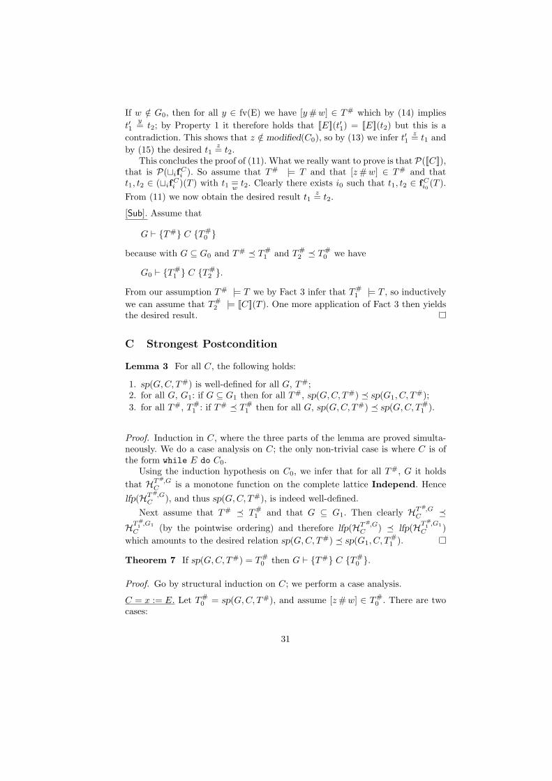
C Strongest Postcondition

Lemma 3 For all C, the following holds:

1. sp(G, C, T#) is well-defined for all G, T#;2. for all G, G1: if G ⊆ G1 then for all T#, sp(G, C, T#) � sp(G1, C, T#);3. for all T#, T#

1 : if T# � T#1 then for all G, sp(G, C, T#) � sp(G, C, T#

1 ).

Proof. Induction in C, where the three parts of the lemma are proved simulta-neously. We do a case analysis on C; the only non-trivial case is where C is ofthe form while E do C0.

Using the induction hypothesis on C0, we infer that for all T#, G it holdsthat HT#,G

C is a monotone function on the complete lattice Independ. Hencelfp(HT#,G

C ), and thus sp(G, C, T#), is indeed well-defined.Next assume that T# � T#

1 and that G ⊆ G1. Then clearly HT#,GC �

HT#1 ,G1

C (by the pointwise ordering) and therefore lfp(HT#,GC ) � lfp(HT#

1 ,G1

C )which amounts to the desired relation sp(G, C, T#) � sp(G1, C, T#

1 ).

Theorem 7 If sp(G, C, T#) = T#0 then G ` {T#} C {T#

0 }.

Proof. Go by structural induction on C; we perform a case analysis.

C = x := E. Let T#0 = sp(G, C, T#), and assume [z # w] ∈ T#

0 . There are twocases:

31

– if z 6= x then [z # w] ∈ T#.– if z = x then w /∈ G, and ∀y ∈ fv(E) • [y # w] ∈ T#.

This establishes G ` {T#} C {T#0 }.

C = C1 ;C2. Assume that sp(G, C1 ;C2, T#) = T#

0 because T#0 = sp(G, C2, T

#1 )

where T#1 = sp(G, C1, T

#). By the induction hypothesis on C1 and on C2, wehave

G ` {T#} C1 {T#1 } and G ` {T#

1 } C2 {T#0 }

from which we infer the desired relation G ` {T#} C1 ;C2 {T#0 }.

C = if E then C1 else C2. Assume that sp(G, if E then C1 else C2, T#) =

T#0 because G0 = G ∪ {w | ∃x ∈ fv(E) • [x# w] /∈ T#}, T#

1 = sp(G0, C1, T#)

and T#2 = sp(G0, C2, T

#) and T#0 = T#

1 ∩ T#2 . Inductively, we have

G0 ` {T#} C1 {T#1 } and G0 ` {T#} C2 {T#

2 }.

As T#0 ⊆ T#

1 and T#0 ⊆ T#

2 we have T#1 � T#

0 and T#2 � T#

0 ; by [Sub], thisimplies

G0 ` {T#} C1 {T#0 } and G0 ` {T#} C2 {T#

0 }.

This establishes the desired G ` {T#} if E then C1 else C2 {T#0 }, since G ⊆

G0 and w /∈ G0 implies ∀x ∈ fv(E) • [x# w] ∈ T#.

C = while E do C0. Assume that sp(G, C, T#) = T#0 so we want to prove G `

{T#} C {T#0 }. We have T#

0 = lfp(HT#,GC ). By definition of a fixed point, T#

0 =HT#,G

C (T#0 ). Thus T#

0 = sp(G0, C0, T#0 ) ∩ T# where G0 = G ∪ {w | ∃x ∈

fv(E) • [x# w] /∈ T#0 }. Hence sp(G0, C0, T

#0 ) � T#

0 and T# � T#0 . We claim

G ` {T#0 } C {T#

0 }, which by [Sub] implies the desired G ` {T#} C {T#0 }.

It remains to prove the claim, G ` {T#0 } C {T#

0 }. By the induction hypoth-esis on C0, G0 ` {T#

0 } C0 {sp(G0, C0, T#0 )} and by [Sub] therefore

G0 ` {T#0 } C0 {T#

0 }.

Now we get G ` {T#0 } C {T#

0 } by an application of [While] because G ⊆ G0

and because w /∈ G0 implies ∀x ∈ fv(E) • [x# w] ∈ T#0 .

Theorem 8 For all judgements G ` {T#1 } C {T#}, sp(G, C, T#

1 ) � T#.

Proof. We perform induction in the derivation of G ` {T#1 } C {T#}, and do a

case analysis on the last rule applied:

[Sub]. Assume that G ` {T#1 } C {T#} because with G ⊆ G1 and T#

1 � T#2 and

T#3 � T# we have G1 ` {T#

2 } C {T#3 }. Applying the induction hypothesis on

that derivation, we get

32

sp(G1, C, T#2 ) � T#

3 .

and by Lemma 3 we get sp(G, C, T#1 ) � sp(G1, C, T#

2 ). This yields the desiredrelation

sp(G, C, T#1 ) � T#

3 � T#.

[Assign], with C = x := E. Assume that G ` {T#1 } C {T#}, and let T#

0 =sp(G, C, T#

1 ). We want T#0 � T#. Accordingly, assume [y # w] ∈ T# to show

[y # w] ∈ T#0 . We have two cases:

– x 6= y. Then [y # w] ∈ T#1 ; hence [y # w] ∈ T#

0 by the definition of sp.– x = y. Then w /∈ G and ∀z ∈ fv(E) • [z # w] ∈ T#

1 ; hence [y # w] ∈ T#0 by

the definition of sp.

[Seq], with C = C1 ;C2. Assume G ` {T#1 } C {T#} because G ` {T#

1 } C1 {T#2 }

and G ` {T#2 } C2 {T#}. By the induction hypothesis on these derivations,

sp(G, C1, T#1 ) � T#

2 and sp(G, C2, T#2 ) � T#

which by Lemma 3 enables us to infer thatsp(G, C2, sp(G, C1, T

#1 )) � T#.

This is as desired, since sp(G, C1 ;C2, T#1 ) = sp(G, C2, sp(G, C1, T

#1 )).

[If], with C = if E then C1 else C2. Assume that G ` {T#1 } C {T#} because

G1 ` {T#1 } C1 {T#} and G1 ` {T#

1 } C2 {T#} where G ⊆ G1 and where w /∈ G1

implies that ∀x ∈ fv(E) • [x# w] ∈ T#1 . Inductively, via the judgements for C1

and C2, we obtainsp(G1, C1, T

#1 ) � T# and sp(G1, C2, T

#1 ) � T#.

Let G0 = G ∪ {w | ∃x ∈ fv(E) • [x# w] /∈ T#1 }. Note that G0 ⊆ G1. Thus by

Lemma 3 we getsp(G0, C1, T

#1 ) � T# and sp(G0, C2, T

#1 ) � T#.

This yields the claim since sp(G, C, T#1 ) = sp(G0, C1, T

#1 ) ∩ sp(G0, C2, T

#1 ).

[While], with C = while E do C0. Assume that G ` {T#} C {T#} becauseG1 ` {T#} C0 {T#} where G ⊆ G1 and where

w /∈ G1 implies that ∀x ∈ fv(E) • [x# w] ∈ T#.

Assume sp(G, C, T#) = T#0 to show T#

0 � T#. By the definition of sp, T#0 =

lfp(HT#,GC ). Inductively, sp(G1, C0, T

#) � T#.Now HT#,G

C (T#) = sp(G0, C0, T#) ∩ T# where G0 = G ∪ {w | ∃x ∈ fv(E) •

[x# w] /∈ T#}. Note that G0 ⊆ G1. Thus, using Lemma 3,

HT#,GC (T#) = (sp(G0, C0, T

#) ∩ T#) � (sp(G1, C0, T#) ∩ T#) = T#.

This shows that HT#,GC is reductive at T#, so by Tarski’s theorem we infer the

desired relation T#0 = lfp(HT#,G

C ) � T#.

33

D Modularity and the Frame Rule

Lemma 4 If y /∈ modified(C) then [y # w] ∈ T# implies [y # w] ∈ sp(G, C, T#).

Proof. Go by structural induction on C; we perform a case analysis. In eachcase, our assumption is that y /∈ modified(C) and that [y # w] ∈ T#; we mustshow [y # w] ∈ sp(G, C, T#).

C = x := E. Our assumptions imply that y 6= x, from which the result triviallyfollows.

C = C1 ;C2. Since y /∈ modified(C1) we can apply the induction hypothesis onC1, giving us [y # w] ∈ sp(G, C1, T

#). Since y /∈ modified(C2) we can then applythe induction hypothesis on C2, giving us [y # w] ∈ sp(G, C2, sp(G, C1, T

#)).This yields the claim.

C = if E then C1 else C2. Since y /∈ modified(C1) and y /∈ modified(C2), wecan apply the induction hypothesis twice, yielding (using the terminology inFig. 3)

[y # w] ∈ T#1 and [y # w] ∈ T#

2 .

Since sp(G, C, T#) = T#1 ∩ T#

2 , this yields the claim.

C = while E do C0. Let T#0 = sp(G, C, T#), then T#

0 = lfp(HT#,GC ). Define

T#1 = T#

0 ∪ {[y # w]}.

By applying the induction hypothesis on C0 (possible since y /∈ modified(C0))we realize that

[y # w] ∈ HT#,GC (T#

1 ). (1)

Since HT#,GC is a monotone function (cf. the proof of Lemma 3), we from T#

1 �T#

0 infer that HT#,GC (T#

1 ) � HT#,GC (T#

0 ) = T#0 and thus

T#0 ⊆ HT#,G

C (T#1 ) (2)

Combining (1) and (2), we infer T#1 ⊆ HT#,G

C (T#1 ), that is HT#,G

C (T#1 ) � T#

1 .This shows that HT#,G

C is reductive at T#1 , so by Tarski’s theorem we infer

T#0 = lfp(HT#,G

C ) � T#1 , that is T#

1 ⊆ T#0 . This demonstrates that [y # w] ∈ T#

0 ,as desired.

Lemma 5 Let T#0 and C be given, with lhs(T#

0 ) ∩ fv(C) = ∅.Then for all T# and G, sp(G, C, T# ∪ T#

0 ) ⊆ sp(G, C, T#) ∪ T#0 .

34

Proof. Go by structural induction on C; we perform a case analysis.

C = x := E. The claim follows from the following calculation:

sp(G, C, T# ∪ T#0 )

= {[y # w] | y 6= x ∧ [y # w] ∈ T# ∪ T#0 } ∪ {[x# w] | w /∈ G ∧ ∀y ∈ fv(E) • [y # w] ∈ T# ∪ T#

0 }= {[y # w] | y 6= x ∧ [y # w] ∈ T# ∪ T#

0 } ∪ {[x# w] | w /∈ G ∧ ∀y ∈ fv(E) • [y # w] ∈ T#}= T#

0 ∪ {[y # w] | y 6= x ∧ [y # w] ∈ T#} ∪ {[x# w] | w /∈ G ∧ ∀y ∈ fv(E) • [y # w] ∈ T#}= T#

0 ∪ sp(G, C, T#)

C = C1 ;C2. Using our induction hypothesis and Lemma 3, we get

sp(G, C, T# ∪ T#0 ) = sp(G, C2, sp(G, C1, T

# ∪ T#0 ))

⊆ sp(G, C2, sp(G, C1, T#) ∪ T#

0 )

⊆ sp(G, C2, sp(G, C1, T#)) ∪ T#

0

= sp(G, C, T#) ∪ T#0

C = if E then C1 else C2. Let

G0 = G ∪ {w | ∃x ∈ fv(E) • [x# w] /∈ T# ∪ T#0 }

and observe that our assumptions imply that also

G0 = G ∪ {w | ∃x ∈ fv(E) • [x# w] /∈ T#}.

Using the induction hypothesis, we now get

sp(G, C, T# ∪ T#0 ) = sp(G0, C1, T

# ∪ T#0 ) ∩ sp(G0, C2, T

# ∪ T#0 )

⊆ (sp(G0, C1, T#) ∪ T#

0 ) ∩ (sp(G0, C2, T#) ∪ T#

0 )

= (sp(G0, C1, T#) ∩ sp(G0, C2, T

#)) ∪ T#0

= sp(G, C, T#) ∪ T#0

C = while E do C0. Let H = HT#,GC and let H0 = HT#∪T#

0 ,G

C , we must showthat

lfp(H0) ⊆ lfp(H) ∪ T#0 .

Define T#1 = lfp(H0), and let

G0 = G ∪ {w | ∃x ∈ fv(E) • [x# w] /∈ T#1 \ T#

0 }

where as above, our assumptions imply that also

G0 = G ∪ {w | ∃x ∈ fv(E) • [x# w] /∈ T#1 }.

35

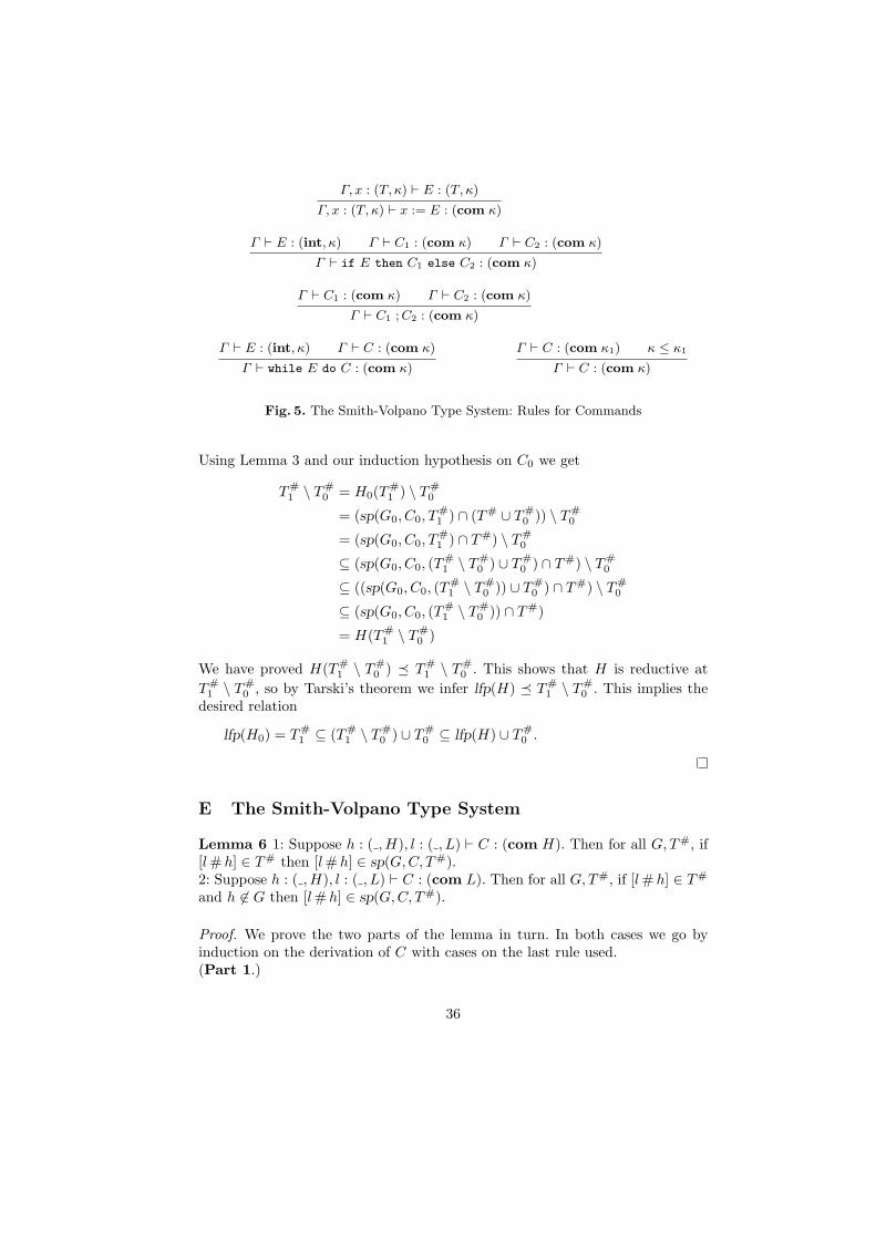
Γ, x : (T, κ) ` E : (T, κ)

Γ, x : (T, κ) ` x := E : (com κ)

Γ ` E : (int, κ) Γ ` C1 : (com κ) Γ ` C2 : (com κ)

Γ ` if E then C1 else C2 : (com κ)

Γ ` C1 : (com κ) Γ ` C2 : (com κ)

Γ ` C1 ; C2 : (com κ)

Γ ` E : (int, κ) Γ ` C : (com κ)

Γ ` while E do C : (com κ)

Γ ` C : (com κ1) κ ≤ κ1

Γ ` C : (com κ)

Fig. 5. The Smith-Volpano Type System: Rules for Commands

Using Lemma 3 and our induction hypothesis on C0 we get

T#1 \ T#

0 = H0(T#1 ) \ T#

0

= (sp(G0, C0, T#1 ) ∩ (T# ∪ T#

0 )) \ T#0

= (sp(G0, C0, T#1 ) ∩ T#) \ T#

0

⊆ (sp(G0, C0, (T#1 \ T#

0 ) ∪ T#0 ) ∩ T#) \ T#

0

⊆ ((sp(G0, C0, (T#1 \ T#

0 )) ∪ T#0 ) ∩ T#) \ T#

0

⊆ (sp(G0, C0, (T#1 \ T#

0 )) ∩ T#)

= H(T#1 \ T#

0 )

We have proved H(T#1 \ T#

0 ) � T#1 \ T#

0 . This shows that H is reductive atT#

1 \ T#0 , so by Tarski’s theorem we infer lfp(H) � T#

1 \ T#0 . This implies the

desired relation

lfp(H0) = T#1 ⊆ (T#

1 \ T#0 ) ∪ T#

0 ⊆ lfp(H) ∪ T#0 .

E The Smith-Volpano Type System

Lemma 6 1: Suppose h : ( ,H), l : ( , L) ` C : (com H). Then for all G, T#, if[l # h] ∈ T# then [l # h] ∈ sp(G, C, T#).2: Suppose h : ( ,H), l : ( , L) ` C : (com L). Then for all G, T#, if [l # h] ∈ T#

and h 6∈ G then [l # h] ∈ sp(G, C, T#).

Proof. We prove the two parts of the lemma in turn. In both cases we go byinduction on the derivation of C with cases on the last rule used.(Part 1.)

36

C = z := E. Clearly, z 6= l as otherwise the assignment cannot be typed. Bydefinition,

sp(G, z := E, T#) ⊇ {[u # w] | u 6= z ∧ [u # w] ∈ T#} 3 [l # h]

C = C1 ;C2. We have h : ( ,H), l : ( , L) ` C1 : (com H) and h : ( ,H), l :( , L) ` C2 : (com H). Inductively, we get,

[l # h] ∈ sp(G, C1, T#) and [l # h] ∈ sp(G, C2, sp(G, C1, T

#))

Thus [l # h] ∈ sp(G, C1 ;C2, T#).

C = if E then C1 else C2. Then h : ( ,H), l : ( , L) ` C1 : (com H) andh : ( ,H), l : ( , L) ` C2 : (com H). Assume [l # h] ∈ T#. Inductively,

[l # h] ∈ sp(G0, C1, T#) and [l # h] ∈ sp(G0, C2, T

#)

where G0 = G∪{w | ∃x ∈ fv(E)• [x# w] /∈ T#}. Thus [l # h] ∈ sp(G0, C1, T#)∩

sp(G0, C2, T#) and we are done.

C = while E do C0. Then h : ( ,H), l : ( , L) ` C0 : (com H). Let T#0 =

sp(G, C, T#). Then T#0 = lfp(HT#,G

C ). Hence T#0 = HT#,G

C (T#0 ).

Let T#1 = T#

0 ∪ [l # h]. Now

HT#,GC (T#

1 ) = sp(G0, C0, T#1 ) ∩ T#, where

G0 = G ∪ {w | ∃x ∈ fv(E) • [x# w] /∈ T#1 }. Inductively, as [l # h] ∈ T#

1 , we get,[l # h] ∈ sp(G0, C0, T

#1 ). Thus,

[l # h] ∈ HT#,GC (T#

1 ). (1)

Because HT#,GC is a monotone function, from T#

1 � T#0 we get HT#,G

C (T#1 ) �

HT#,GC (T#

0 ) = T#0 . Thus

T#0 ⊆ HT#,G

C (T#1 ). (2)

Combining (1) and (2), we get T#1 ⊆ HT#,G

C (T#1 ), i.e., HT#,G

C (T#1 ) � T#

1 .This shows that HT#,G

C is reductive at T#1 , so by Tarski’s theorem, T#

0 =lfp(HT#,G

C ) � T#1 , that is, T#

1 ⊆ T#0 . Hence [l # h] ∈ T#

0 .

Subtyping. For the subtyping rule, the result trivially follows by induction onthe smaller derivation tree for C.This completes Part 1 of the proof.(Part 2.)

Subtyping. Assume [l # h] ∈ T# and h 6∈ G. By the typing rule, h : ( ,H), l :( , L) ` C : (com L) follows because h : ( ,H), l : ( , L) ` C : (com κ1) for anyκ1. If κ1 = L, the result follows inductively. If κ1 = H, then we can apply Part

37

1 of the theorem to conclude that [l # h] ∈ T# holds for any G; in particular, itmust therefore hold for the G where h 6∈ G.

C = z := E. Assume [l # h] ∈ T# and h 6∈ G. By typing, z : ( , L) (so z 6= h)and h 6∈ fv(E), as otherwise the assignment cannot be typed. Hence z = l. Bydefinition,5

sp(G, z := E, T#) ⊇ {[z # w] | w /∈ G ∧ ∀u ∈ fv(E) • [u # w] ∈ T#} 3 [l # h]

C = C1 ;C2. Easy induction.

C = if E then C1 else C2. By typing, h : ( ,H), l : ( , L) ` E : (int, L). Henceh 6∈ fv(E). Hence, h 6∈ G0, where G0 = G ∪ {w | ∃x ∈ fv(E) • [x# w] /∈ T#}.Thus inductively, using the definition of sp, we obtain [l # h] ∈ sp(G0, C1, T

#)and [l # h] ∈ sp(G0, C2, T

#). Hence [l # h] ∈ sp(G0, C1, T#) ∩ sp(G0, C2, T

#).

C = while E do C0. By typing, h : ( ,H), l : ( , L) ` E : (int, L). Hence h 6∈fv(E). Now the proof proceeds similarly to the corresponding case in Part 1 andis omitted; we note that to use the induction hypothesis on the derivation of C0,we only need to show h 6∈ G0, where G0 = G ∪ {w | ∃x ∈ fv(E) • [x# w] /∈ T#

1 }.But this follows since h 6∈ G and h 6∈ fv(E).

F Counter-example Generation

Our main goal is to prove Lemma 7, but first a few auxiliary results:

Fact 14 Assume that t′ = [[C]]I(t). Then tx= t′ for all x /∈ modified(C). And

for all x ∈ Var, either tx= t′ or tg-t′(x) ∈ C.

The proof is an easy structural induction in C.

Definition 5. We say that C modifies y wrt. I if for all t ∈ Trc, tg-t′(y) ∈ Cwhere t′ = [[C]]I(t).

Lemma 10. Assume that y ∈ modified(C). Then there exists I covering C suchthat C modifies y wrt. I.

Proof. Structural induction in C, with three cases:

C = τ : x := E. We infer that y = x, and the claim is immediate.

C = C1 ;C2. There are two possibilities:y ∈ modified(C2). We apply the induction hypothesis on C2, and find I2

covering C2 such that C2 modifies y wrt. I2. Let I be an arbitrary extension of5 In case there are several low variables, we would use the argument:

sp(G, z := E, T#) ⊇ {[u # w] | u 6= z ∧ [u # w] ∈ T#} 3 [l # h]

to deal with low variables not assigned to.

38

I2 that covers C. We shall show that C modifies y wrt. I, so let t be given andlet t′ = [[C]]I(t). There exists t1 such that t′ = [[C2]]I(t1) = [[C2]]I2(t1), so sinceC2 modifies y wrt. I2 we infer that tg-t′(y) ∈ C2 and therefore tg-t′(y) ∈ C.

y ∈ modified(C1) and y /∈ modified(C2). We apply the induction hypothesison C1, and find I1 covering C1 such that C1 modifies y wrt. I1. Let I be anarbitrary extension of I1 that covers C. We shall show that C modifies y wrt.I, so let t be given and let t′ = [[C]]I(t). We have t′ = [[C2]]I(t1) where t1 =[[C1]]I(t) = [[C1]]I1(t), and since C1 modifies y wrt. I1 we infer that tg-t1(y) ∈ C1.From Fact 14 applied to C2 we infer that t′

y= t1, showing tg-t′(y) ∈ C1 and

therefore tg-t′(y) ∈ C.

C = if τ : E then C1 else C2. Wlog. we can assume that y ∈ modified(C1).We then apply the induction hypothesis on C1 and find I1 covering C1 suchthat C1 modifies y wrt. I1. Let I be an extension of I1 that covers C such thatI(tgτ (v)) holds for all v. We shall show that C modifies y wrt. I, so let t be givenand let t′ = [[C]]I(t). Due to our choice of I, we have t′ = [[C1]]I(t) = [[C1]]I1(t).Since C1 modifies y wrt. I1, this yields tg-t′(y) ∈ C1 and therefore the desiredtg-t′(y) ∈ C.

We are now ready to prove Lemma 7:Lemma 7 Assume that with h /∈ G we have sp(G, C, T#) = T#

0 , and assumethat [y # h] /∈ T#

0 . Then there exists z such that [z # h] /∈ T#, and such that Creveals y using z.

Proof. Structural induction in C, with three cases:

C = τ : x := E. There are two subcases:y = x. Since h /∈ G, we infer that there exists z ∈ fv(E) such that [z # h] /∈

T#. We shall show that C does indeed reveal y using z, so consider t1, t2 with¬(t1

z= t2). From Property 2 we infer that [[E]](t1) 6= [[E]](t2) and thus alsotgτ ([[E]](t1)) 6= tgτ ([[E]](t2)) (since otherwise we could apply un-tg on both sidesand get a contradiction). With I the empty interpretation, this implies thedesired ¬([[C]]I(t1)

y= [[C]]I(t2)).

y 6= x. We infer that [y # h] /∈ T#, and it is trivial that C does indeed revealy using y.

C = C1 ;C2. There exists T#1 such that sp(G, C1, T

#) = T#1 and sp(G, C2, T

#1 ) =

T#0 . Inductively on C2, we can find x such that [x# h] /∈ T#

1 and such that C2

reveals y using x. Inductively on C1, we can then find z such that [z # h] /∈ T#

and such that C1 reveals x using z.We must show that C reveals y using z, so let t1 and t2 be given where

t1 ∆ C and t2 ∆ C and where ¬(t1z= t2).

We have already established that C1 reveals x using z, so since t1 ∆ C1 andt2 ∆ C1 we can find an interpretation function I1 covering C1 such that

¬([[C1]]I1(t1)x= [[C1]]I1(t2)).

39

By Fact 14, we see that [[C1]]I1(t1) ∆ C2 and [[C1]]I1(t2) ∆ C2. So since we haveestablished that C2 reveals y using x, we can find I2 covering C2 such that

¬([[C2]]I2([[C1]]I1(t1))y= [[C2]]I2([[C1]]I1(t2))).

With I the union of I1 and I2, this amounts to the desired relation ¬([[C]]I(t1)y=

[[C]]I(t2)).

C = if τ : E then C1 else C2. There exists T#1 and T#

2 with T#0 = T#

1 ∩ T#2

such that sp(G0, C1, T#) = T#

1 and sp(G0, C2, T#) = T#

2 where G0 = G ∪ {w |∃x ∈ fv(E) • [x# w] /∈ T#}. Given y with [y # h] /∈ T#

0 , either [y # h] /∈ T#1 or

[y # h] /∈ T#2 ; wlog. we may assume that [y # h] /∈ T#

1 . We split into three cases.h /∈ G0. We can apply the induction hypothesis on C1, to find z such that

[z # h] /∈ T# and such that C1 reveals y using z. We shall show that also C

reveals y using z, so consider t1 and t2 where ¬(t1z= t2) and with t1 ∆ C and

t2 ∆ C.Since C1 reveals y using z, there exists I1 covering C1 such that ¬([[C1]]I1(t1)

y=

[[C1]]I1(t2)). Let I be an extension of I1 that covers C such that I(tgτ (v)) holdsfor all v. Then [[C]]I(t1) = [[C1]]I1(t1) and [[C]]I(t2) = [[C1]]I1(t2), yielding thedesired relation ¬([[C]]I(t1)

y= [[C]]I(t2)).

y /∈ modified(C1). Since [y # h] /∈ sp(G0, C1, T#), Lemma 4 tells us that

[y # h] /∈ T#. We shall show that C reveals y using y. So consider t1 and t2where ¬(t1

y= t2) and with t1 ∆ C and t2 ∆ C. Let I cover C such that

I(tgτ (v)) holds for all v. By Fact 14 we have [[C1]]I(t1)y= t1 and [[C1]]I(t2)

y=

t2, implying ¬([[C1]]I(t1)y= [[C1]]I(t2)) which amounts to the desired relation

¬([[C]]I(t1)y= [[C]]I(t2)).

h ∈ G0, y ∈ modified(C1). From h ∈ G0 we infer that there exists z ∈ fv(E)such that [z # h] /∈ T#. We shall show that C reveals y using z, so considert1 and t2 where t1 ∆ C and t2 ∆ C and where ¬(t1

z= t2), by Property 2implying [[E]](t1) 6= [[E]](t2). By Lemma 10, there exists I1 covering C1 such thatC1 modifies y wrt. I1. Now define an interpretation function I that covers Cand that has the following properties (which are always possible to obtain): Iextends I1; I(tgτ ([[E]](t1))) is true; I(tgτ ([[E]](t2))) is false. Let

t′1 = [[C]]I(t1) = [[C1]]I1(t1)t′2 = [[C]]I(t2) = [[C2]]I(t2).

Since C1 modifies y wrt. I1, tg-t′1(y) ∈ C1. By Fact 14, we see that either t2y= t′2

or tg-t′2(y) ∈ C2; in both cases our assumptions (t2 ∆ C and unique tagging)imply tg-t′2(y) /∈ C1. This shows the desired relation ¬(t′1

y= t′2).

40