Information Extraction Principles and Methods for ...landgreb/Principles.pdfMultispectral...
30
© 1998 by David Landgrebe. Copying for personal or non-commercial educational use of this material is permitted. However, permission to reprint/republish this material for advertising or promotional purposes or for creating other new collective works for resale or redistribution to servers or lists, or to reuse any copyrighted component of this work in other works must be obtained from David Landgrebe and the World Scientific Publishing Company. This work was originally prepared for and appears in Information Processing for Remote Sensing , edited by C. H. Chen, published by the World Scientific Publishing Co., Inc., 1060 Main Street, River Edge, NJ 07661, USA (Spring, 1999). In addition to general works such as this one, this book contains sections on Pattern Recognition, SAR Image Processing and Segmentation, Parameter Extraction, Neural Network and Fuzzy Logic Methods, Change Detection, Knowledge-based Methods and Data Fusion, Image Processing Algorithms including wavelet analysis techniques, Image Compression, and Discrimination of Buried Objects. Information Extraction Principles and Methods for Multispectral and Hyperspectral Image Data David Landgrebe School of Electrical & Computer Engineering Purdue University, West Lafayette, IN 47907-1285 Voice: 765-494-3486 Fax: 765-494-3358 [email protected] Introduction In the U.S., the era of space-based multispectral remote sensing of land areas began soon after the launch of the first Earth satellite in 1957 and the creation of NASA in 1959. Satellites to observe the weather became an initial focus of Earth-looking satellites, with the first U.S. satellite designed for that purpose launched in 1960. Research on land remote sensing began soon thereafter and was initially focused on the Earth’s renewable and non-renewable resources, and especially on food and fiber production. The need envisioned was very much use-driven, as compared to a purely scientific interest. The primary objective of the early research was to create a practical but especially, an economical technology to supply usable and needed information about the Earth’s resources for both application and scientific interests. Vertical views of the Earth’s land surface provide a unique vantagepoint, one different than ordinary human experience. The world does not look the same from altitude looking down. But it is not so much the simple uniqueness of this vantagepoint that was the attractive feature as the fact that from altitude one can see more, thus suggesting the economic value of the synoptic view and the ability to cover large areas quickly and inexpensively. On the other hand, this raises the question of dealing with large quantities of data. This motivation and line of thinking led to considering ways to collect information via a space platform from image data with the lowest spatial resolution usable. The spatial resolution of a spaceborne sensor is one of the more expensive parameters. Higher spatial resolution leads not only to larger quantities of data for a given area as resolution is increased, but to larger (thus heavier) sensor systems, increased precision requirements on spacecraft guidance and control, wider bandwidth downlinks, and the like. This is what led to the concept of using spectral measurements of a pixel to identify what ground cover the pixel represents, rather than to use spatial variations (imagery) and more conventional image processing techniques, methods which generally require higher spatial resolution. For similar reasons, methods were pursued which marry the unique capabilities of both human and computer. Rather than seeking a fully “automatic” system, it appeared to be much wiser to attempt to construct a data analysis scheme that takes advantage of keen perceptive and associative powers of the human in conjunction with the objective quantitative abilities of computers. Fully manual systems in the form of air photo interpretation had been used for many years. Though a great deal of work has gone into fully machine implemented systems, the problem of devising completely automatic schemes has proved to be quite daunting with only limited success even to the current time. The most functional schemes that have become available in a practical sense can perhaps best be described as human assisted machine processing schemes. Where the focus has been placed on “image enhancement,” such systems might be labeled machine assisted human schemes. In the following we will focus on the human assisted machine approach. Indeed, there is a down side to even seeking a fully automatic system. As compared to a machine, the human has exceptional
-
Upload
hoangquynh -
Category
Documents
-
view
216 -
download
0
Transcript of Information Extraction Principles and Methods for ...landgreb/Principles.pdfMultispectral...

© 1998 by David Landgrebe. Copying for personal or non-commercial educational use of this material is permitted.However, permission to reprint/republish this material for advertising or promotional purposes or for creatingother new collective works for resale or redistribution to servers or lists, or to reuse any copyrighted component ofthis work in other works must be obtained from David Landgrebe and the World Scientific Publishing Company.This work was originally prepared for and appears in Informat ion Process ing for Remote Sens ing , editedby C. H. Chen, published by the World Scientific Publishing Co., Inc., 1060 Main Street, River Edge, NJ 07661,USA (Spring, 1999). In addition to general works such as this one, this book contains sections on PatternRecognition, SAR Image Processing and Segmentation, Parameter Extraction, Neural Network and Fuzzy LogicMethods, Change Detection, Knowledge-based Methods and Data Fusion, Image Processing Algorithms includingwavelet analysis techniques, Image Compression, and Discrimination of Buried Objects.
Information Extraction Principles and Methodsfor Multispectral and Hyperspectral Image Data
David LandgrebeSchool of Electrical & Computer Engineering
Purdue University, West Lafayette, IN 47907-1285Voice: 765-494-3486 Fax: 765-494-3358
IntroductionIn the U.S., the era of space-based multispectral remote sensing of land areas began soon after thelaunch of the first Earth satellite in 1957 and the creation of NASA in 1959. Satellites to observethe weather became an initial focus of Earth-looking satellites, with the first U.S. satellite designedfor that purpose launched in 1960. Research on land remote sensing began soon thereafter and wasinitially focused on the Earth’s renewable and non-renewable resources, and especially on foodand fiber production. The need envisioned was very much use-driven, as compared to a purelyscientific interest. The primary objective of the early research was to create a practical butespecially, an economical technology to supply usable and needed information about the Earth’sresources for both application and scientific interests. Vertical views of the Earth’s land surfaceprovide a unique vantagepoint, one different than ordinary human experience. The world does notlook the same from altitude looking down. But it is not so much the simple uniqueness of thisvantagepoint that was the attractive feature as the fact that from altitude one can see more, thussuggesting the economic value of the synoptic view and the ability to cover large areas quickly andinexpensively. On the other hand, this raises the question of dealing with large quantities of data.
This motivation and line of thinking led to considering ways to collect information via a spaceplatform from image data with the lowest spatial resolution usable. The spatial resolution of aspaceborne sensor is one of the more expensive parameters. Higher spatial resolution leads notonly to larger quantities of data for a given area as resolution is increased, but to larger (thusheavier) sensor systems, increased precision requirements on spacecraft guidance and control,wider bandwidth downlinks, and the like. This is what led to the concept of using spectralmeasurements of a pixel to identify what ground cover the pixel represents, rather than to usespatial variations (imagery) and more conventional image processing techniques, methods whichgenerally require higher spatial resolution.
For similar reasons, methods were pursued which marry the unique capabilities of both human andcomputer. Rather than seeking a fully “automatic” system, it appeared to be much wiser to attemptto construct a data analysis scheme that takes advantage of keen perceptive and associative powersof the human in conjunction with the objective quantitative abilities of computers. Fully manualsystems in the form of air photo interpretation had been used for many years. Though a great dealof work has gone into fully machine implemented systems, the problem of devising completelyautomatic schemes has proved to be quite daunting with only limited success even to the currenttime. The most functional schemes that have become available in a practical sense can perhaps bestbe described as human assisted machine processing schemes. Where the focus has been placed on“image enhancement,” such systems might be labeled machine assisted human schemes. In thefollowing we will focus on the human assisted machine approach. Indeed, there is a down side toeven seeking a fully automatic system. As compared to a machine, the human has exceptional
Multispectral Information Extraction Principles
1998 by David Landgrebe 2 11/9/98
perceptive powers and abilities to abstract and to generalize. A fully automatic system would haveto forego these capabilities, and thus is likely to be more limited and less robust in its abilities andperhaps less economical as well.
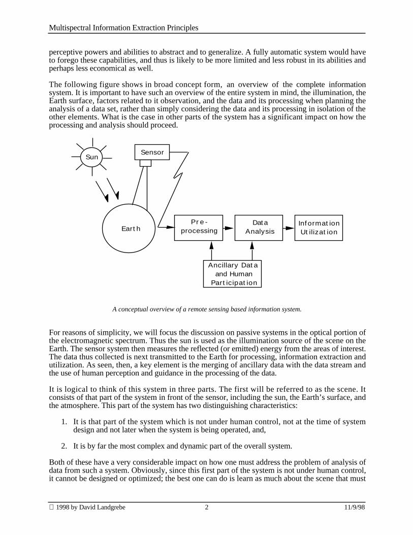
The following figure shows in broad concept form, an overview of the complete informationsystem. It is important to have such an overview of the entire system in mind, the illumination, theEarth surface, factors related to it observation, and the data and its processing when planning theanalysis of a data set, rather than simply considering the data and its processing in isolation of theother elements. What is the case in other parts of the system has a significant impact on how theprocessing and analysis should proceed.
Sun
Earth
Sensor
P re -processing
DataAnalysis
InformationUtilization
Ancillary Data and Human
Participation
A conceptual overview of a remote sensing based information system.
For reasons of simplicity, we will focus the discussion on passive systems in the optical portion ofthe electromagnetic spectrum. Thus the sun is used as the illumination source of the scene on theEarth. The sensor system then measures the reflected (or emitted) energy from the areas of interest.The data thus collected is next transmitted to the Earth for processing, information extraction andutilization. As seen, then, a key element is the merging of ancillary data with the data stream andthe use of human perception and guidance in the processing of the data.
It is logical to think of this system in three parts. The first will be referred to as the scene. Itconsists of that part of the system in front of the sensor, including the sun, the Earth’s surface, andthe atmosphere. This part of the system has two distinguishing characteristics:
1. It is that part of the system which is not under human control, not at the time of systemdesign and not later when the system is being operated, and,
2. It is by far the most complex and dynamic part of the overall system.
Both of these have a very considerable impact on how one must address the problem of analysis ofdata from such a system. Obviously, since this first part of the system is not under human control,it cannot be designed or optimized; the best one can do is learn as much about the scene that must
Multispectral Information Extraction Principles
1998 by David Landgrebe 3 11/9/98
be dealt with as possible. In addition, then, the complexity of the scene and its dynamism dictateswhat types of approaches to scene models and what data analysis approaches might be useful. It isvery easy to underestimate this complexity and dynamism of the scene and to undertake toosimplistic an approach to data analysis, thus limiting the robustness of the procedure and theaccuracy and detail of the information that can result. For example, the spectral response of a giventype of vegetation may be expected to change significantly from day to day due to growth andmaturity factors, prior weather conditions, and the like. It may be expected to change even fromminute to minute and from one part of a scene to another due to wind effects, the sun angle-viewangle combination, and other variables. In general, one cannot count on a vegetative canopy havinga stable “spectral signature.”
The second part of the system is the sensor portion. This portion of the system is characterized bythe fact that, though it is under human design control, it is usually not under the control of theanalyst at the time of data acquisition. Thus, the analyst must pretty much accept what is given, interms of the parameters of the data produced, i.e., the spectral and spatial resolution, thequantization precision, the sensor field of view and look angle and the like. Though the systemdesigner may select these characteristics in the process of optimizing the system for a certain classof uses, the individual user usually does not have a choice of them for the particular application,site, and time of season in mind.
It is the third part of the system, all of that after arrival of the data at the processing point, overwhich the analyst has the greatest control. Thus it is here that choices can be made with regard toalgorithm selection and operation to optimize performance to the specific data set and use. In theremainder of this chapter, we will explore the factors that go into making these choices.
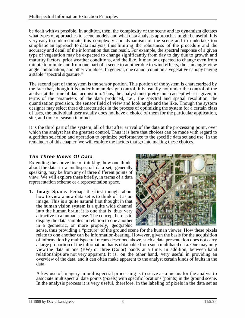
The Three Views Of DataExtending the above line of thinking, how one thinksabout the data in a multispectral data set, generallyspeaking, may be from any of three different points ofview. We will explore these briefly, in terms of a datarepresentation scheme or a representation space.
1 . Image Space. Perhaps the first thought abouthow to view a new data set is to think of it as animage. This is a quite natural first thought in thatthe human vision system is a quite wide channelinto the human brain; it is one that is thus veryattractive in a human sense. The concept here is todisplay the data samples in relation to one anotherin a geometric, or more properly, geographicsense, thus providing a “picture” of the ground scene for the human viewer. How these pixelsrelate to one another can be information-bearing. However, given the basis for the acquisitionof information by multispectral means described above, such a data presentation does not carrya large proportion of the information that is obtainable from such multiband data. One may onlyview the data in one (BW) or three (Color) bands at a time. In addition, between bandrelationships are not very apparent. It is, on the other hand, very useful in providing anoverview of the data, and it can often make apparent to the analyst certain kinds of faults in thedata.
A key use of imagery in multispectral processing is to serve as a means for the analyst toassociate multispectral data points (pixels) with specific locations (points) in the ground scene.In the analysis process it is very useful, therefore, in the labeling of pixels in the data set as

Multispectral Information Extraction Principles
1998 by David Landgrebe 4 11/9/98
training samples, i.e., examples of the classes that the analyst wishes to identify.Fundamentally, the analysis process consists of bringing together the wishes of the analyst interms of what classes are desired with the scene spectral properties as expressed in the data.One cannot expect a satisfactory final product unless the analyst can carefully and completelydefine which spectral properties are intended to belong to which classes. The training samplesare the means for doing this. Thus the means for allowing the analyst to accomplish this is thekey to successful analysis. As will be seen, this fundamental step becomes even more crucialfor hyperspectral data.
The spatial relationships available in an image expression of multispectral data has also beenfound effective in a limited way as an adjunct to spectral relationships in extracting informationfrom the data.
2. Spectral Space. The emergence of the multispectralconcept began to focus attention on how the responsemeasured in an individual pixel varies as a function ofwavelength as an information-bearing aspect, andindeed, perhaps the key such aspect. The idea is that, ifresponse vs. wavelength effectively conveys neededinformation by which to identify the contents of anindividual pixel, this provides a fundamental simplicitythat is important from a processing economics point ofview. In this circumstance, pixels can be processed oneat a time, a much simpler arrangement than would beneeded using so-called picture processing or image processing schemes. It is inherently moresuited to the computer and quantitative representation of data. Further, compared to imageprocessing schemes, being able to label each pixel individually results in a higher resolutionresult than, for example, a label associated with a neighborhood of pixels, as would be the casefor conventional image processing schemes.
Response as a function of wavelength has the very useful characteristic that it provides theanalyst with spectral information that is often directly interpretable. Especially when a highdegree of spectral detail is present, characteristics of a given pixel response can be related tophysical properties of the contents of the pixel area. For example, one can easily tell whether apixel contains vegetation, soil, or water. In the case of high-resolution spectra, one may evenbe able to identify a particular molecule based upon the location of specific absorption bands, ina manner similar to that used by chemical spectroscopists in the laboratory. Thus, for theanalyst, a display of spectral response can provide a direct link to physical properties. For thisreason, fundamental scientists tend to initiate their thinking about multispectral data from thepoint of view of spectral space. In limited cases, such spectral curves may be used directly inmachine implemented spectral matching schemes.
But viewing a graph of response vs. wavelength for an individual pixel does not provide thewhole story so far as the relationship between spectral response and information available fromthe scene is concerned. The spectral response of any given Earth surface cover type tends tovary in a characteristic way. The spectral response of corn field pixels at a given time, forexample, is not uniform for all the pixels of the field, but varies in a characteristic way aboutsome mean value. This is due to the relationships between the size and mixture of leaves,stalks, soil background, the physiology of the plants, etc, leading to different mixtures ofilluminated and shadowed surfaces and the like. This variation is, to a useful degree, diagnosticof the plant species and thus useful in discriminating between corn and the other plant speciesthat may be in the scene. But such variation, though present in the spectral responses from thefield, is not easily discernable from a presentation of a series of plots of response vs.

Multispectral Information Extraction Principles
1998 by David Landgrebe 5 11/9/98
wavelength for the class. For this purpose, the third form of data expression, the feature spaceproves more useful, especially in relation to machine processing.
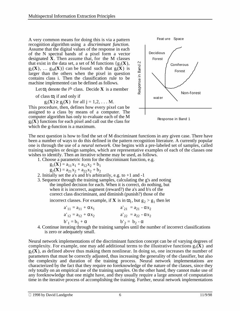
3. Feature Space. If one samples the spectral response at two different wavelengths, λ1 and λ2as shown above, the values resulting can be plotted as shown at right, thus creating a 2-dimensional display. If one samples at more values of λ, for example, 10 values of λ, the pointrepresenting each spectral response would then be a point in 10-dimensional space. This turnsout to be an especially useful way of representing spectralresponses. If one samples the spectrum at enoughwavelengths, so that one could reconstruct the spectralcurve from the samples, the information the spectralresponse contains is preserved, and it is now representedas a vector. Though one cannot show such a pointgraphically, a computer can more easily deal it with thanwith a graph.
Further, this is a mathematical representation of what amultispectral sensor does, i.e. sampling the spectralresponse in each of N spectral bands. The result is then anN-dimensional vector containing all the available spectral information about that pixel. Theadvantage of this type of representation is that it is a quantitative way of representing not onlythe numerical values of individual pixels, but also how the values for a given material may varyabout their central or mean value. As indicated above, this turns out to often be quite diagnosticof the material. We shall deal more fully with this fact later.
Each of these three data spaces, then, has its advantages and limitations. Image space shows therelationship of spectral response to its geographic position, and it provides a way to associate eachpixel with a location on the ground. It also provides some additional information useful in analysis.Spectral space often enables one to relate a given spectral response to the type of material it resultsfrom. Feature space provides a representation especially convenient for machine processing, forexample, by use of a pattern recognition algorithm. It is this latter method of data analysis, a verycommon one for multispectral analysis, we will explore next, using it as a means for exploringhow information is contained in spectral data, and how it may be extracted.
Analysis Algorithms And the Relationship With Ancillary DataWe next consider the process of analysis or extracting information from the data. The term dataanalysis can mean many things in different applications. A common one is to make a thematic mapof the scene by associating a class label with each pixel of the scene. For simplicity, we will focuson that objective. In terms of feature space, one might think of the analysis process as that ofdelineating the region of the feature space associated with each class of interest. For example, onemight somehow determine which region of the space contains spectral values associated withwheat, which part contains forest pixels, which contains urban pixels and the like. In terms of thethematic map concept, this means partitioning up the feature space such that each possible locationin the space has a unique class label associated with it.
Multispectral Information Extraction Principles
1998 by David Landgrebe 6 11/9/98
A very common means for doing this is via a patternrecognition algorithm using a discriminant function.Assume that the digital values of the response in eachof the N spectral bands of a pixel form a vectordesignated X . Then assume that, for the M classesthat exist in the data set, a set of M functions {g1(X ),g2(X ), … gM(X )} can be found such that gi(X ) islarger than the others when the pixel in questioncontains class i. Then the classification rule to bemachine implemented can be defined as follows.
Let ωi denote the ith class. Decide X is a member
of class ωi if and only ifgi(X ) ≥ gj(X ) for all j = 1,2, . . . M.
This procedure, then, defines how every pixel can beassigned to a class by means of a computer. Thecomputer algorithm has only to evaluate each of the Mgi(X ) functions for each pixel and call out the class forwhich the g-function is a maximum.
The next question is how to find the set of M discriminant functions in any given case. There havebeen a number of ways to do this defined in the pattern recognition literature. A currently popularone is through the use of a neural network. One begins with a pre-labeled set of samples, calledtraining samples or design samples, which are representative examples of each of the classes onewishes to identify. Then an iterative scheme may be used, as follows.
1. Choose a parametric form for the discriminant function, e.g.g1(X ) = a11x1 + a12x2 + b1g2(X ) = a21x2 + a22x2 + b2
2. Initially set the a's and b's arbitrarily, e.g. to +1 and -13. Sequence through the training samples, calculating the g's and noting
the implied decision for each. When it is correct, do nothing, butwhen it is incorrect, augment (reward?) the a's and b's of thecorrect class discriminant, and diminish (punish?) those of theincorrect classes. For example, if X is in ω1, but g2 > g1 then let
a'11 = a11 + αx1 a'21 = a21 - αx2
a'12 = a12 + αx2 a'22 = a22 - αx2
b'1 = b1 + α b'2 = b2 - α4. Continue iterating through the training samples until the number of incorrect classifications
is zero or adequately small.
Neural network implementations of the discriminant function concept can be of varying degrees ofcomplexity. For example, one may add additional terms to the illustrative functions g1(X ) andg2(X ), as defined above thus making them nonlinear. In doing so, one increases the number ofparameters that must be correctly adjusted, thus increasing the generality of the classifier, but alsothe complexity and duration of the training process. Neural network implementations arecharacterized by the fact that they require no foreknowledge of the nature of the classes, since theyrely totally on an empirical use of the training samples. On the other hand, they cannot make use ofany foreknowledge that one might have, and they usually require a large amount of computationtime in the iterative process of accomplishing the training. Further, neural network implementations
waterNon-forest
Decidious
Forest
Coniferous
Forest
Response in Band 1
Feature Space

Multispectral Information Extraction Principles
1998 by David Landgrebe 7 11/9/98
do not lend themselves to analytical evaluation very easily. It is more difficult to predict theperformance, for example, and therefore to adjust the configuration and parameters to an optimum.
A second common approach to determining a set of discriminant functions utilizes a statisticalapproach. The training samples, instead of being used in an empirical calculation as above, areused to evaluate a probabilistic model for each class. That is, they can be used to estimate theprobability density function associated with each class. Recall that the value of a probability densityfunction at any point indicates the relative likelihood of that point. Thus, by using class probabilitydensity functions as discriminant functions, one is deciding in favor of the most likely class foreach pixel.
More formally, let p(X |ωi) be the (N-dimensional) probability density function for class i, and
p(ωi) be the probability that class i occurs in the data set. Then, the decision rule becomes:
Decide X is in class ωi if and only if
p(X |ωi)p(ωi) ≥ p(X |ωj)p(ωj) for all j = 1,2,...,m
This decision rule is known as the Bayes Rule, and it can be shown that it provides the minimumprobability of error for the density functions used.
Any of a wide variety of probabilistic models can be used, in either parametric or non-parametricform. Often the density for the classes can be assumed to be normally or Gaussianly distributed. Inthis case, the class probability density function becomes,
p(X |ωi) = (2π)-N/2 |Σ i|-1/2 exp{-1/2 (X - X i)T Σ i
-1 (X - X i) }
where X i is the class mean value and Σ i is its covariance matrix. In this case, one has only to usethe training samples to estimate the class mean vectors and covariance matrices, a very shortcalculation.
Furthermore, if the Gaussian assumption is applicable, as it often is, due in part to the CentralLimit Theorem, significant simplification of the process can be made. If p(X |ωi)p(ωi) ≥p(X |ωj)p(ωj) for all j = 1,2,...,M, then it is also true that
ln p(X |ωi)p(ωi) ≥ ln p(X |ωj)p(ωj) for all j = 1,2,...,M. Thus one may take the following as an equivalent discriminant function, but one that requiressubstantially less computation time. (Note in this expression that we have dropped the factorinvolving 2π since it would be common to all class discriminant functions and thus does notcontribute to the discrimination.)
gi(X ) = ln p(ωi) - (1/2)ln|Σ i| - (1/2)(X - X i )TΣ i-1(X - X i )
or 2gi(X ) = ln p2(ωi)
|Σ i| - (X - X i )TΣ i
-1(X - X i )
Note also that the first term on the right must only be computed once per class, and only the lastterm must be computed for each pixel to be classified. The calculation that must be implemented isthus quite straightforward and simple.
Thus, to achieve optimal performance, one must (a) have good estimates of the class mean vectorsand covariance matrices, after having (b) chosen an appropriate probability model and a proper setof classes. These conditions turn out to be the key ones to achieving good results. We shall nextexplore these two conditions more fully.
Multispectral Information Extraction Principles
1998 by David Landgrebe 8 11/9/98
(a) On the importance of accurate class statistics. One of the defining circumstances ofthe remote sensing problem is the fact that training samples are usually not as numerous as wouldbe desirable. As it turns out, this factor has a strong relationship to the number of spectral bandscontained in the measurement and the signal-to-noise ratio of the sensor. That is to say that thenumber of training samples needed to adequately define the classes quantitatively, regardless ofwhat discriminant function implementation is used, grows very rapidly with the number of spectralbands to be used. To understand how this influences the performance, we begin by drawingattention to the following long-standing theoretical result. 1
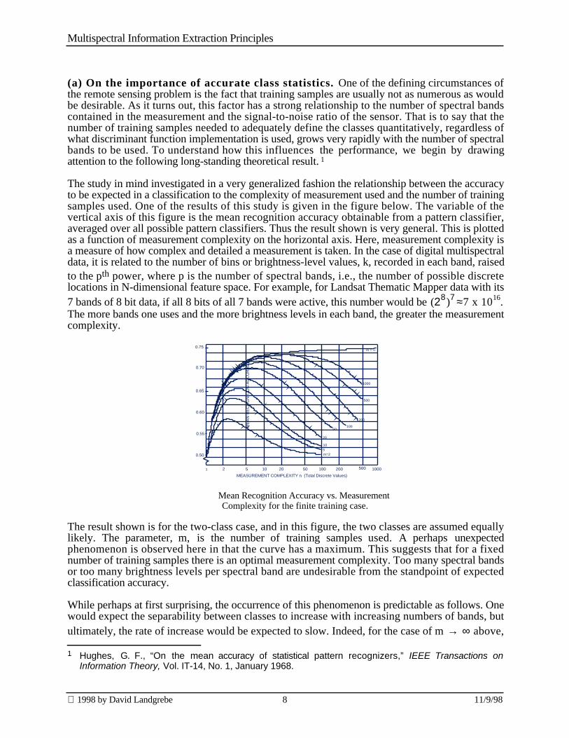
The study in mind investigated in a very generalized fashion the relationship between the accuracyto be expected in a classification to the complexity of measurement used and the number of trainingsamples used. One of the results of this study is given in the figure below. The variable of thevertical axis of this figure is the mean recognition accuracy obtainable from a pattern classifier,averaged over all possible pattern classifiers. Thus the result shown is very general. This is plottedas a function of measurement complexity on the horizontal axis. Here, measurement complexity isa measure of how complex and detailed a measurement is taken. In the case of digital multispectraldata, it is related to the number of bins or brightness-level values, k, recorded in each band, raisedto the pth power, where p is the number of spectral bands, i.e., the number of possible discretelocations in N-dimensional feature space. For example, for Landsat Thematic Mapper data with its7 bands of 8 bit data, if all 8 bits of all 7 bands were active, this number would be (28)7 ≈7 x 10¹⁶.The more bands one uses and the more brightness levels in each band, the greater the measurementcomplexity.
m=2510
20
50100
200
1000
500
m = ∞
1 100050020010050201052
MEASUREMENT COMPLEXITY n (Total Discrete Values)
0.50
0.55
0.60
0.65
0.70
0.75
ME
AN
RE
CO
GN
ITIO
N A
CC
UR
AC
Y
Mean Recognition Accuracy vs. MeasurementComplexity for the finite training case.
The result shown is for the two-class case, and in this figure, the two classes are assumed equallylikely. The parameter, m, is the number of training samples used. A perhaps unexpectedphenomenon is observed here in that the curve has a maximum. This suggests that for a fixednumber of training samples there is an optimal measurement complexity. Too many spectral bandsor too many brightness levels per spectral band are undesirable from the standpoint of expectedclassification accuracy.
While perhaps at first surprising, the occurrence of this phenomenon is predictable as follows. Onewould expect the separability between classes to increase with increasing numbers of bands, butultimately, the rate of increase would be expected to slow. Indeed, for the case of m → ∞ above, 1 Hughes, G. F., “On the mean accuracy of statistical pattern recognizers,” IEEE Transactions on
Information Theory, Vol. IT-14, No. 1, January 1968.

Multispectral Information Extraction Principles
1998 by David Landgrebe 9 11/9/98
the probably accuracy rises rapidly at first, but eventually becomes asymptotic to 0.75, aprobability half between 0.5 (chance performance) and 100%. For a fixed, finite numbers oftraining samples, one would expect the accuracy with which one could estimate the classdistribution would decrease as the measurement complexity grows. For example, in the case ofGaussian statistics, the number of parameters to be estimated in the covariance matrix growsrapidly with dimensionality, and the preciseness needed would grow with the increased detail asthe number of digital bins grows. Thus there are two counterbalancing effects, one increasing withincreasing measurement complexity and the other decreasing. The shape of the above curve isexplained, then, by the fact that first the former effect dominates but eventually the latter does so,thus a maximum occurs.
It is significant to note that the value of the maximum in this curve moves upward and to the rightas m is increased. The practical implication of this is that one can expect to be able to increaseaccuracy by using increased numbers of bands and/or signal-to-noise ratio, but to achieve it,increased numbers of training samples, implying increased precision in the estimation of classdistributions, will be needed. This observation becomes increasingly important as one moves fromlower dimensional data to hyperspectral data with its many 10’s to several hundreds of bands. Weshall return to this point later.
(b) On defining classes and their probability models. In addition to adequate numbers oftraining samples, the other key factor in successful analysis is the matter of the definition ofclasses. There are three conditions for optimal class definition, as follows.
Optimal class definition requires that the classes defined must be• Exhaustive. There must be a logical class to assign each pixel in the scene to.• Separable. The classes must be separable to an adequate degree in terms of the spectral
features available.• Of informational value. The classes must be ones that meet the users needs.
A few comments about each of these conditions are in order.
Exhaustive. First, relative to the requirement that the class list be exhaustive, it is a basicengineering reality that relative determinations can be made more accurately than can absolute ones.Just as one can measure the distance between two objects more precisely than one can measure theabsolute location of the objects, or one can measure the time between two events more preciselythan one can measure the absolute time of day of the two events, one has a better chance ofassigning a pixel to the correct class if one can consider all possible classes, selecting the bestalternative, than simply trying to identify the class of the pixel without taking into account the otherpossibilities. Thus, one speaks of the classifier being a relative classifier rather than an absoluteclassifier. To have a relative classification scheme, one must have an exhaustive list ofpossibilities, where here exhaustive implies a list of all classes that occur in the specific data set tobe analyzed.
Separable. Clearly, one must have a list of classes that are separable to an adequate degree, for thisis the whole point of the process, the division of the data set into classes of interest. Thus in theanalysis procedure, one must find the most optimal procedure one can to discriminate successfullybetween the classes. This statement has implications not only on the algorithms used in theanalysis, but on the way the classes are defined and training samples drawn in the first place. Morewill be said about this point as procedures for practical analysis are discussed.
Of Informational Value. This is the point at which the user’s requirement is expressed for whatoutput from the analysis is desired. For any given multispectral data set, there are many differenttypes of information that might be desired. For example, over an area with an incomplete canopyof vegetation, one might want to derive a soil map. On the other hand, one might wish to ignore
Multispectral Information Extraction Principles
1998 by David Landgrebe 10 11/9/98
the soil variations as background variation and attempt to obtain a vegetation species map. Variousother possibilities might exist. It is thus in the definition of classes that the user’s specific interestsin the analysis result are expressed.
These three conditions on the list of classes must be met simultaneously. Note that the exhaustivecondition and separability are properties of the data set, while the user imposes the informationalvalue condition. It is the bringing together of these circumstances, those imposed by the data withthose imposed by the user’s desires that is the challenge to the analyst. It is further noted that theclasses are defined by the training samples selected. That is to say that the definition of classes is aquantitative and objective one, not a semantic one. One has not really defined a class one mightwish to call “forest” until one has labeled the training samples to be associated with that classname, thus documenting quantitatively what is meant (and what is not meant) by the word “forest.”
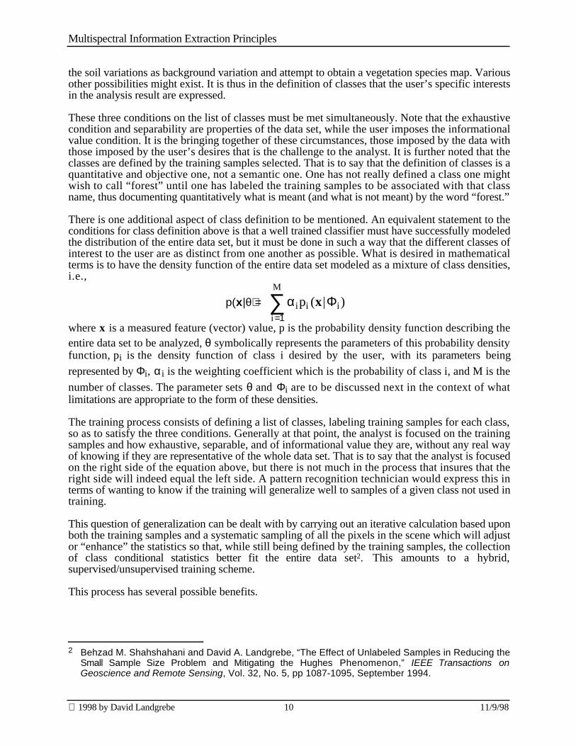
There is one additional aspect of class definition to be mentioned. An equivalent statement to theconditions for class definition above is that a well trained classifier must have successfully modeledthe distribution of the entire data set, but it must be done in such a way that the different classes ofinterest to the user are as distinct from one another as possible. What is desired in mathematicalterms is to have the density function of the entire data set modeled as a mixture of class densities,i.e.,
p(x|θ) = αipi (x |Φi)i=1
M
∑
where x is a measured feature (vector) value, p is the probability density function describing theentire data set to be analyzed, θ symbolically represents the parameters of this probability densityfunction, pi is the density function of class i desired by the user, with its parameters being
represented by Φi, αi is the weighting coefficient which is the probability of class i, and M is the
number of classes. The parameter sets θ and Φi are to be discussed next in the context of whatlimitations are appropriate to the form of these densities.
The training process consists of defining a list of classes, labeling training samples for each class,so as to satisfy the three conditions. Generally at that point, the analyst is focused on the trainingsamples and how exhaustive, separable, and of informational value they are, without any real wayof knowing if they are representative of the whole data set. That is to say that the analyst is focusedon the right side of the equation above, but there is not much in the process that insures that theright side will indeed equal the left side. A pattern recognition technician would express this interms of wanting to know if the training will generalize well to samples of a given class not used intraining.
This question of generalization can be dealt with by carrying out an iterative calculation based uponboth the training samples and a systematic sampling of all the pixels in the scene which will adjustor “enhance” the statistics so that, while still being defined by the training samples, the collectionof class conditional statistics better fit the entire data set2. This amounts to a hybrid,supervised/unsupervised training scheme.
This process has several possible benefits.
2 Behzad M. Shahshahani and David A. Landgrebe, “The Effect of Unlabeled Samples in Reducing the
Small Sample Size Problem and Mitigating the Hughes Phenomenon,” IEEE Transactions onGeoscience and Remote Sensing, Vol. 32, No. 5, pp 1087-1095, September 1994.

Multispectral Information Extraction Principles
1998 by David Landgrebe 11 11/9/98
(1) The process tends to make the training set more robust, providing an improved fitto the entire data set, thus providing improved generalization to data other than thetraining samples.
(2) The process tends to mitigate the Hughes phenomena. Enhancing the statistics bysuch a scheme in effect, tends to increase the size of the training set and thustends to move the peak accuracy vs. number of features to a higher value at ahigher dimensionality, thus allowing one to obtain greater accuracy with a limitedtraining set.
(3) An estimate is obtained for the prior probabilities of the classes, the α’s in theequation above, as a result of the use of the unlabeled samples, something thatcannot be done with the training samples alone. In some cases, where only howmuch of an area contains a given class is desired, and not a map of where itoccurs, this could be the final desired result.
To carry out the process, for each class Sj, assume there are Nj training samples available. Denotethese samples by zjk where j=1,...,J indicates the class of origin and k=1,...,Nj is the index ofeach particular sample. The training samples are assumed to come from a particular class withoutany reference to the exact component within that class. In addition to the training samples, assumeN unlabeled samples, denoted by xk, k=1,...,N, are also available from the mixture.
The process to be followed is referred to as the EM (expectation maximization) algorithm. Theprocedure is to maximize the log likelihood to obtain maximum likelihood estimates of theparameters involved. The log likelihood expression to be maximized can be written in thefollowing form.
L(θ ) = log p (xk |θ )k =1
N
∑ + log1
αtt ∈S j
∑αl pl (z jk | φl )
l ∈S j
∑
k =1
Nj
∑j=1
J
∑
The first term in this function is the likelihood of the unlabeled samples with respect to the mixturedensity. The second term indicates the likelihood of the training samples with respect to theircorresponding classes of origin. The EM equations for obtaining the ML estimates are thefollowing:
αi+ =
P c
k=1
N
∑ (i|xk ) + P jc(i|z jk )
k=1
N j
∑
N(1+N j
Pc
k=1
N
∑ (r|x k )r∈S j
∑)
Multispectral Information Extraction Principles
1998 by David Landgrebe 12 11/9/98
µ i+ =
Pc(i|xk )xk + P jc(i|z jk)z jk
k=1
Nj
∑k=1
N
∑
P c(i|xk ) + P jc(i|z jk )
k=1
N j
∑k=1
N
∑
Σ i+ =
Pc(i|xk )(xk −µ i+)(xk −µ i
+)T + P jc(i|z jk)(z jk
k=1
Nj
∑ −µ i+)(z jk −µ i
+ )T
k=1
N
∑
Pc(i|xk ) + P jc(i|z jk )
k=1
N j
∑k=1
N
∑
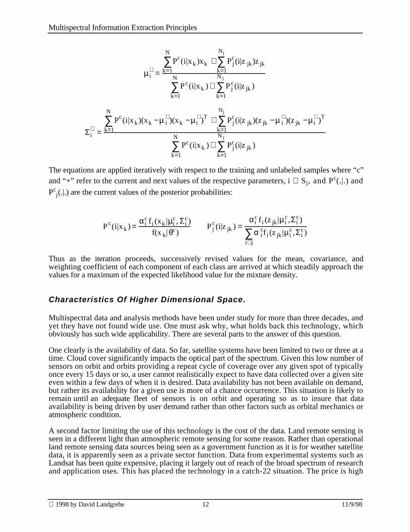
The equations are applied iteratively with respect to the training and unlabeled samples where “c”and “+” refer to the current and next values of the respective parameters, i ∈ Sj, and Pc(.|.) and
Pcj(.|.) are the current values of the posterior probabilities:
P c(i|xk ) =αi
c f i (xk |µic , Σ i
c)
f(x k| θc) P j
c(i|z jk ) =αi
c f i (z jk |µ ic ,Σ i
c)
α icf i (z jk |µ i
c ,Σ ic)
i∈j∑
Thus as the iteration proceeds, successively revised values for the mean, covariance, andweighting coefficient of each component of each class are arrived at which steadily approach thevalues for a maximum of the expected likelihood value for the mixture density.
Characteristics Of Higher Dimensional Space.
Multispectral data and analysis methods have been under study for more than three decades, andyet they have not found wide use. One must ask why, what holds back this technology, whichobviously has such wide applicability. There are several parts to the answer of this question.
One clearly is the availability of data. So far, satellite systems have been limited to two or three at atime. Cloud cover significantly impacts the optical part of the spectrum. Given this low number ofsensors on orbit and orbits providing a repeat cycle of coverage over any given spot of typicallyonce every 15 days or so, a user cannot realistically expect to have data collected over a given siteeven within a few days of when it is desired. Data availability has not been available on demand,but rather its availability for a given use is more of a chance occurrence. This situation is likely toremain until an adequate fleet of sensors is on orbit and operating so as to insure that dataavailability is being driven by user demand rather than other factors such as orbital mechanics oratmospheric condition.
A second factor limiting the use of this technology is the cost of the data. Land remote sensing isseen in a different light than atmospheric remote sensing for some reason. Rather than operationalland remote sensing data sources being seen as a government function as it is for weather satellitedata, it is apparently seen as a private sector function. Data from experimental systems such asLandsat has been quite expensive, placing it largely out of reach of the broad spectrum of researchand application uses. This has placed the technology in a catch-22 situation. The price is high

Multispectral Information Extraction Principles
1998 by David Landgrebe 13 11/9/98
because the volume is low, and the volume is low, at least in part, because the price is high. Again,until the volume builds to a reasonable level, data is likely to be too expensive for most uses.
However, it is the third reason for the limited use to this time that is to be addressed at greaterlength here, because it is a technologically-based limitation rather than a government policy one,and because advancing technology is in the process of removing this third limitation. The limitationin mind is that due to the small number of spectral bands that have been available. The research inthe 1960’s that led to the Landsat system was done using an aircraft system that had from 12 to 18spectral bands of 8 bit data. However, this degree of spectral detail was beyond what wastechnically feasible for Landsat 1, and a four band, 6 bit system resulted. When in 1975 it was timeto devise a second generation sensor, the bar was raised to initially 6 and finally a 7 band, 8 bitsystem, certainly an improvement over four, but still a significant limitation. This limitedmeasurement complexity placed many applications of the technology in a borderline area or simplyout of reach. It has not been until recent years that more complex data, often under the label ofhyperspectral data, began to be studied and planned. Such an advance greatly broadens theproblems that can be realistically addressed, but it also complicates the matter of how to analyzethis more complex data. It is this latter point that will be addressed next. The initial focus is on thenature of high dimensional data and how it differs from more conventional data.
Much of the material in previous sections has been offered in the context of a feature space infamiliar two or three dimensional geometry. However, hyperspectral data has many more thanthree bands, and thus the feature space of interest has much higher dimensionality. One mustinquire as to whether ones ordinary intuitive perception developed from three-dimensionalgeometry still apply in higher dimensional space. The answer is that, in general, it does not, andthis fact substantially influences what is appropriate in the analysis process.
As an example of this, consider the case of predicting the accuracy of a classification from thetraining samples of the classes defined. One of the most common ways of accomplishing such aprediction is by use of a statistical distance measure. Such a distance measure is Bhattacharyyadistance. For the 2-class case of Gaussian data, the definition of Bhattacharyya distance is,
B = 18 [µ1-µ2]T[
Σ1 + Σ2
2]-1[µ1-µ2] +
12 Ln
12
Σ1 + Σ2[ ]Σ1 Σ2
Where µi and Σ i are, respectively, the mean vector and the covariance matrix of class i.
In the multispectral remote sensing context, Bhattacharyya distance has shown itself to be a goodpredictor of classification accuracy. Though there is not a closed form, one-to-one relationshipbetween Bhattacharyya distance and classification accuracy, the following graph shows the resultof a Monte Carlo test of this relationship for the two-class, two-feature case.

Multispectral Information Extraction Principles
1998 by David Landgrebe 14 11/9/98
It is seen that in this case, the relationship is nearly one-to-one, and nearly linear.
Examining the equation defining it, one sees that of the two terms on the right, the first measuresthe separation of the classes due to the difference in class means. The second does not depend at allon the difference in means, but measures the portion of the separation due to the difference incovariance matrices. In low dimensional space, where geometric visualization is possible, the meanvector defines the location of a distribution in the feature space while the covariance matrixprovides information about its shape. For example, a covariance matrix with significantly sizedoff-diagonal components indicating significant correlation between bands would tend geometricallyto be long and narrow, while a covariance matrix with only small off-diagonal components, andthus low correlation between bands, would tend to be more circular in shape. Now, oneimplication of this is that two classes may lie precisely on top of one another, in the sense ofhaving exactly the same mean values, and yet they may be separable. Indeed, if the dimensionalityis high enough, they may be quite separable. It turns out that this is especially true as thedimensionality is increased. Why might this be so?
What is needed is a more in-depth understanding of such unintuitive characteristics of highdimensional feature spaces. We will review a selection of these unusual or unexpectedcharacteristics3, because they point the way to some practical procedures for data analysis thatmight not be otherwise apparent.
A. As dimensionality increases the volume of a hypercube concentrates in the corners.
The volume of the hypersphere of radius r and dimension d is known to be given by the equation:
Vs r( ) = Volume of a hypersphere =2r d
d
πd
2
Γ d2
(1)
3 Jimenez, Luis, and David Landgrebe, “Supervised Classification in High Dimensional Space:
Geometrical, Statistical, and Asymptotical Properties of Multivariate Data,” IEEE Transactions onSystem, Man, and Cybernetics, Volume 28 Part C Number 1, pp. 39-54, Feb. 1998.
Multispectral Information Extraction Principles
1998 by David Landgrebe 15 11/9/98
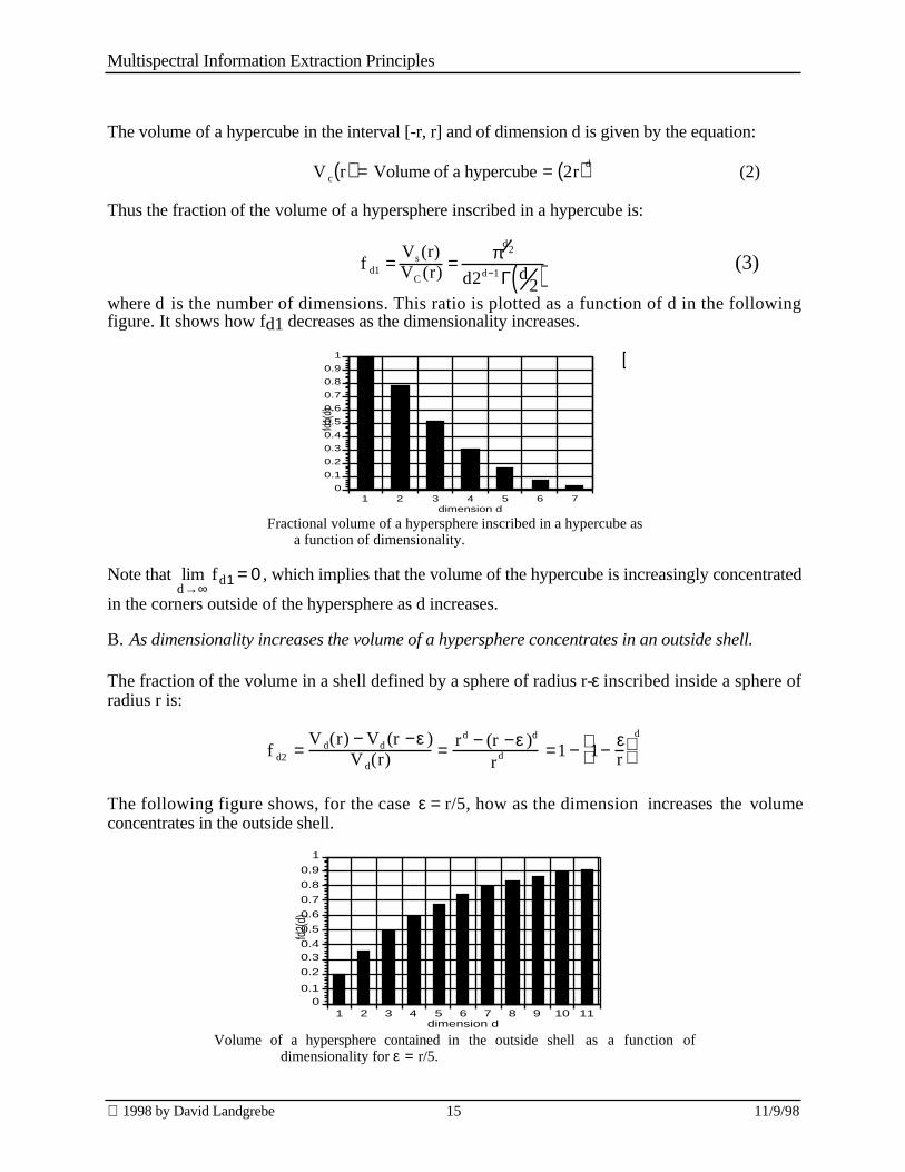
The volume of a hypercube in the interval [-r, r] and of dimension d is given by the equation:
V c r( ) = Volume of a hypercube = 2r( )d(2)
Thus the fraction of the volume of a hypersphere inscribed in a hypercube is:
f d1 =Vs (r)VC (r) = π
d2
d2d−1 Γ d2( ) (3)
where d is the number of dimensions. This ratio is plotted as a function of d in the followingfigure. It shows how fd1 decreases as the dimensionality increases.
1 2 3 4 5 6 70
0.1
0.2
0.3
0.4
0.5
0.6
0.7
0.8
0.9
1
fd1(
d)
dimension d
Fractional volume of a hypersphere inscribed in a hypercube asa function of dimensionality.
Note that limd→∞
fd1 = 0 , which implies that the volume of the hypercube is increasingly concentrated
in the corners outside of the hypersphere as d increases.
B. As dimensionality increases the volume of a hypersphere concentrates in an outside shell.
The fraction of the volume in a shell defined by a sphere of radius r-ε inscribed inside a sphere ofradius r is:
f d2 =V d(r) − Vd (r −ε )
V d(r) = rd − (r −ε )d
rd =1 − 1− εr
d
The following figure shows, for the case ε = r/5, how as the dimension increases the volumeconcentrates in the outside shell.
1 2 3 4 5 6 7 8 9 10 110
0.1
0.2
0.30.4
0.5
0.6
0.7
0.8
0.9
1
fd2(
d)
dimension d
Volume of a hypersphere contained in the outside shell as a function ofdimensionality for ε = r/5.

Multispectral Information Extraction Principles
1998 by David Landgrebe 16 11/9/98
Note that d →∞lim f d2 = 1 for any ε > 0, implying that most of the volume of a hypersphere is
concentrated in an outside shell, away from the center of the spheres.
These characteristics have two important consequences that bear upon practical methods for dataanalysis. First, higher dimensional space is mostly empty, which implies that the multivariate datain any given case is usually in a lower dimensional structure. This implies that a high dimensionaldata set can be projected to a lower dimensional subspace without losing significant information interms of separability among the different statistical classes. The second consequence of theforegoing, is that normally distributed data will have a tendency to concentrate in the tails;similarly, uniformly distributed data will be more likely to be collected in the corners, makingdensity estimation more difficult. Local neighborhoods are almost surely empty, requiring thebandwidth of estimation to be large and producing the effect of losing detailed density estimation.
Support for this tendency can be found in the statistical behavior of normally and uniformlydistributed multivariate data at high dimensionality. It is expected that as the dimensionalityincreases the data will concentrate in an outside shell. As the number of dimensions increases thatshell will increase its distance from the origin as well. A quantitative demonstration of thesecharacteristics is given in [4,5].
The tendency for Gaussian data to concentrate in the tails seems like a paradox, since it is clearfrom the Gaussian density function that the “most likely” values are near the mean, not in the tails?This paradox can be explained as follows6. First note what happens to the magnitude of a zeromean Gaussian density function as the dimensionality increases. This is shown in the followinggraph.
0 1 2 3 4 50
0.1
0.2
0.3
0.4
Distance from Class Mean, r
n=1
2
3
4 5
n: dimensionality
It is seen that, while the shape of the curve remains bell-shaped, its magnitude becomes smallerwith increasing dimensionality, as it must, since the overall volume must remain one, and, ofcourse, it decreases exponentially as r increases.
4 Jimenez, Luis, and David Landgrebe, “Supervised Classification in High Dimensional Space:
Geometrical, Statistical, and Asymptotical Properties of Multivariate Data,” IEEE Transactions onSystem, Man, and Cybernetics, Volume 28 Part C Number 1, pp. 39-54, Feb. 1998.
5 Luis O. Jimenez and David Landgrebe, “High Dimensional Feature Reduction Via Projection Pursuit,”PhD thesis and School of Electrical & Computer Engineering Technical Report TR-ECE 96-5, April1996.
6 This explanation was provided by graduate student Pi-fuei Hsieh.
Multispectral Information Extraction Principles
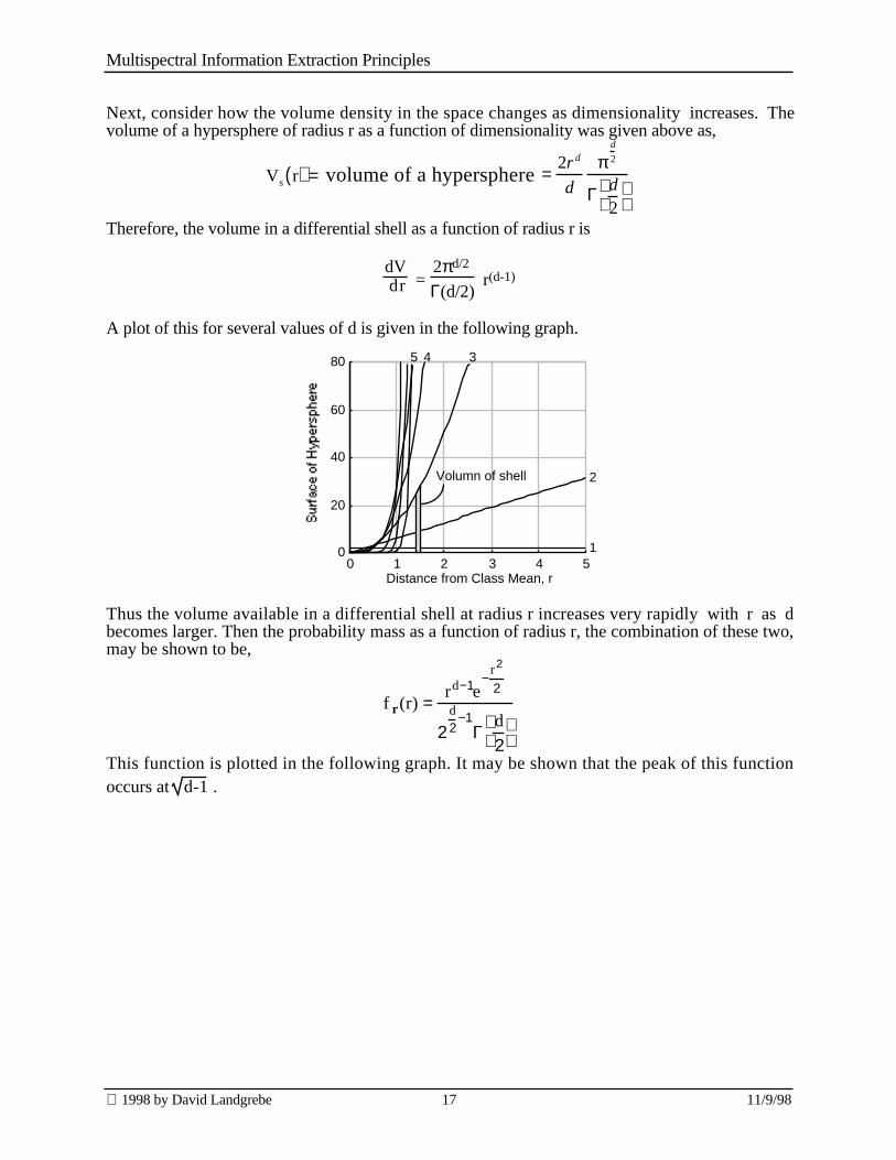
1998 by David Landgrebe 17 11/9/98
Next, consider how the volume density in the space changes as dimensionality increases. Thevolume of a hypersphere of radius r as a function of dimensionality was given above as,
Vs r( ) = volume of a hypersphere =2r d
d
πd
2
Γ d2
Therefore, the volume in a differential shell as a function of radius r is
dV dr =
2πd/2
Γ(d/2) r(d-1)
A plot of this for several values of d is given in the following graph.
0 1 2 3 4 50
20
40
60
80
Distance from Class Mean, r
1
2
3 4 5
Volumn of shell
Thus the volume available in a differential shell at radius r increases very rapidly with r as dbecomes larger. Then the probability mass as a function of radius r, the combination of these two,may be shown to be,
f r(r) =rd−1e
−r2
2
2d2
−1Γ
d
2
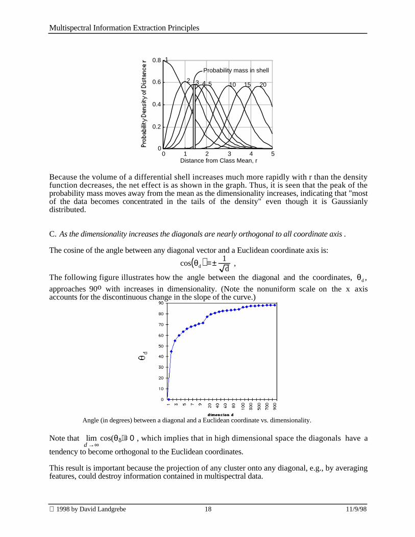
This function is plotted in the following graph. It may be shown that the peak of this functionoccurs at d-1 .
Multispectral Information Extraction Principles
1998 by David Landgrebe 18 11/9/98
0 1 2 3 4 50
0.2
0.4
0.6
0.8
Distance from Class Mean, r
1
2 3 4 5 10 15 20
Probability mass in shell
Because the volume of a differential shell increases much more rapidly with r than the densityfunction decreases, the net effect is as shown in the graph. Thus, it is seen that the peak of theprobability mass moves away from the mean as the dimensionality increases, indicating that "mostof the data becomes concentrated in the tails of the density" even though it is Gaussianlydistributed.
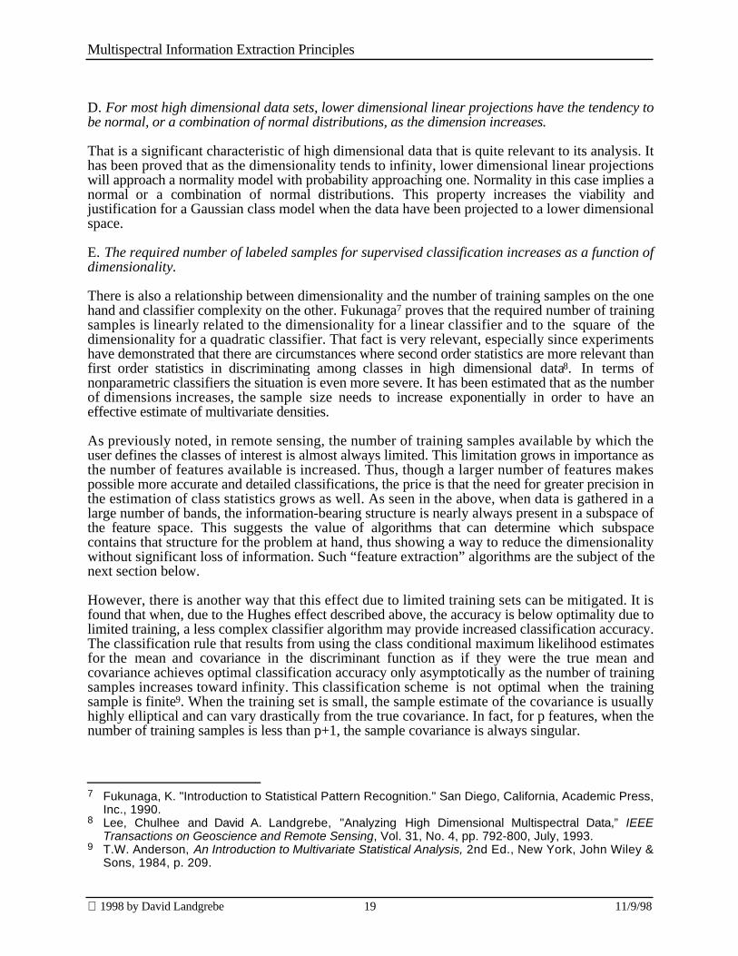
C. As the dimensionality increases the diagonals are nearly orthogonal to all coordinate axis .
The cosine of the angle between any diagonal vector and a Euclidean coordinate axis is:
cos θd( ) =± 1d
,
The following figure illustrates how the angle between the diagonal and the coordinates, θd ,
approaches 90o with increases in dimensionality. (Note the nonuniform scale on the x axisaccounts for the discontinuous change in the slope of the curve.)
Angle (in degrees) between a diagonal and a Euclidean coordinate vs. dimensionality.
Note that limd →∞
cos(θδ) = 0, which implies that in high dimensional space the diagonals have a
tendency to become orthogonal to the Euclidean coordinates.
This result is important because the projection of any cluster onto any diagonal, e.g., by averagingfeatures, could destroy information contained in multispectral data.
Multispectral Information Extraction Principles
1998 by David Landgrebe 19 11/9/98
D. For most high dimensional data sets, lower dimensional linear projections have the tendency tobe normal, or a combination of normal distributions, as the dimension increases.
That is a significant characteristic of high dimensional data that is quite relevant to its analysis. Ithas been proved that as the dimensionality tends to infinity, lower dimensional linear projectionswill approach a normality model with probability approaching one. Normality in this case implies anormal or a combination of normal distributions. This property increases the viability andjustification for a Gaussian class model when the data have been projected to a lower dimensionalspace.
E. The required number of labeled samples for supervised classification increases as a function ofdimensionality.
There is also a relationship between dimensionality and the number of training samples on the onehand and classifier complexity on the other. Fukunaga7 proves that the required number of trainingsamples is linearly related to the dimensionality for a linear classifier and to the square of thedimensionality for a quadratic classifier. That fact is very relevant, especially since experimentshave demonstrated that there are circumstances where second order statistics are more relevant thanfirst order statistics in discriminating among classes in high dimensional data8. In terms ofnonparametric classifiers the situation is even more severe. It has been estimated that as the numberof dimensions increases, the sample size needs to increase exponentially in order to have aneffective estimate of multivariate densities.
As previously noted, in remote sensing, the number of training samples available by which theuser defines the classes of interest is almost always limited. This limitation grows in importance asthe number of features available is increased. Thus, though a larger number of features makespossible more accurate and detailed classifications, the price is that the need for greater precision inthe estimation of class statistics grows as well. As seen in the above, when data is gathered in alarge number of bands, the information-bearing structure is nearly always present in a subspace ofthe feature space. This suggests the value of algorithms that can determine which subspacecontains that structure for the problem at hand, thus showing a way to reduce the dimensionalitywithout significant loss of information. Such “feature extraction” algorithms are the subject of thenext section below.
However, there is another way that this effect due to limited training sets can be mitigated. It isfound that when, due to the Hughes effect described above, the accuracy is below optimality due tolimited training, a less complex classifier algorithm may provide increased classification accuracy.The classification rule that results from using the class conditional maximum likelihood estimatesfor the mean and covariance in the discriminant function as if they were the true mean andcovariance achieves optimal classification accuracy only asymptotically as the number of trainingsamples increases toward infinity. This classification scheme is not optimal when the trainingsample is finite9. When the training set is small, the sample estimate of the covariance is usuallyhighly elliptical and can vary drastically from the true covariance. In fact, for p features, when thenumber of training samples is less than p+1, the sample covariance is always singular.
7 Fukunaga, K. "Introduction to Statistical Pattern Recognition." San Diego, California, Academic Press,
Inc., 1990.8 Lee, Chulhee and David A. Landgrebe, "Analyzing High Dimensional Multispectral Data,” IEEE
Transactions on Geoscience and Remote Sensing, Vol. 31, No. 4, pp. 792-800, July, 1993.9 T.W. Anderson, An Introduction to Multivariate Statistical Analysis, 2nd Ed., New York, John Wiley &
Sons, 1984, p. 209.
Multispectral Information Extraction Principles
1998 by David Landgrebe 20 11/9/98
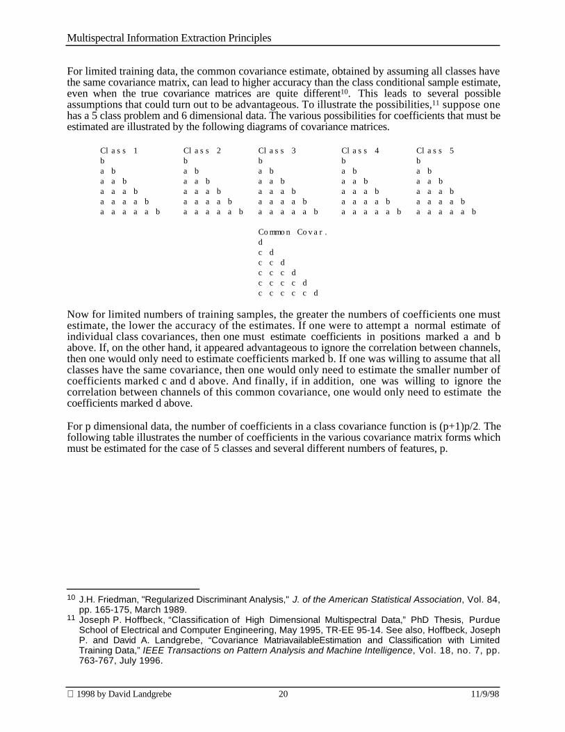
For limited training data, the common covariance estimate, obtained by assuming all classes havethe same covariance matrix, can lead to higher accuracy than the class conditional sample estimate,even when the true covariance matrices are quite different10. This leads to several possibleassumptions that could turn out to be advantageous. To illustrate the possibilities,11 suppose onehas a 5 class problem and 6 dimensional data. The various possibilities for coefficients that must beestimated are illustrated by the following diagrams of covariance matrices.
Class 1 Class 2 Class 3 Class 4 Class 5b b b b ba b a b a b a b a ba a b a a b a a b a a b a a ba a a b a a a b a a a b a a a b a a a ba a a a b a a a a b a a a a b a a a a b a a a a ba a a a a b a a a a a b a a a a a b a a a a a b a a a a a b
Common Covar.dc dc c dc c c dc c c c dc c c c c d
Now for limited numbers of training samples, the greater the numbers of coefficients one mustestimate, the lower the accuracy of the estimates. If one were to attempt a normal estimate ofindividual class covariances, then one must estimate coefficients in positions marked a and babove. If, on the other hand, it appeared advantageous to ignore the correlation between channels,then one would only need to estimate coefficients marked b. If one was willing to assume that allclasses have the same covariance, then one would only need to estimate the smaller number ofcoefficients marked c and d above. And finally, if in addition, one was willing to ignore thecorrelation between channels of this common covariance, one would only need to estimate thecoefficients marked d above.
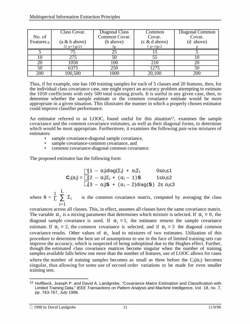
For p dimensional data, the number of coefficients in a class covariance function is (p+1)p/2. Thefollowing table illustrates the number of coefficients in the various covariance matrix forms whichmust be estimated for the case of 5 classes and several different numbers of features, p.
10 J.H. Friedman, "Regularized Discriminant Analysis," J. of the American Statistical Association, Vol. 84,
pp. 165-175, March 1989.11 Joseph P. Hoffbeck, “Classification of High Dimensional Multispectral Data,” PhD Thesis, Purdue
School of Electrical and Computer Engineering, May 1995, TR-EE 95-14. See also, Hoffbeck, JosephP. and David A. Landgrebe, “Covariance MatriavailableEstimation and Classification with LimitedTraining Data,” IEEE Transactions on Pattern Analysis and Machine Intelligence, Vol. 18, no. 7, pp.763-767, July 1996.
Multispectral Information Extraction Principles
1998 by David Landgrebe 21 11/9/98
No. ofFeatures p
Class Covar.
(a & b above)5{ p+1)p/2}
Diagonal ClassCommon Covar.
(b above)5p
CommonCovar.
(c & d above){ p+1)p/2
Diagonal CommonCovar.
(d above)p
5 75 25 15 510 275 50 55 1020 1050 100 210 2050 6375 250 1275 50200 100,500 1000 20,100 200
Thus, if for example, one has 100 training samples for each of 5 classes and 20 features, then, forthe individual class covariance case, one might expect an accuracy problem attempting to estimatethe 1050 coefficients with only 500 total training pixels. It is useful in any given case, then, todetermine whether the sample estimate or the common covariance estimate would be moreappropriate in a given situation. This illustrates the manner in which a properly chosen estimatorcould improve classifier performance.
An estimator referred to as LOOC, found useful for this situation12, examines the samplecovariance and the common covariance estimates, as well as their diagonal forms, to determinewhich would be most appropriate. Furthermore, it examines the following pair-wise mixtures ofestimators:
• sample covariance-diagonal sample covariance,• sample covariance-common covariance, and• common covariance-diagonal common covariance.
The proposed estimator has the following form:
C i(αi) = (1 – αi)diag(Σ i) + αiΣ i 0≤α i≤1
(2 – αi)Σ i + ( αi – 1 )S 1≤α i≤2(3 – αi)S + ( αi – 2)diag(S ) 2≤ αi≤3
where S = 1L ∑
i=1
L Σ i is the common covariance matrix, computed by averaging the class
covariances across all classes. This, in effect, assumes all classes have the same covariance matrix.The variable α i is a mixing parameter that determines which mixture is selected. If αi = 0, thediagonal sample covariance is used. If αi = 1, the estimator returns the sample covarianceestimate. If αi = 2, the common covariance is selected, and if αi = 3 the diagonal commoncovariance results. Other values of α i lead to mixtures of two estimates. Utilization of thisprocedure to determine the best set of assumptions to use in the face of limited training sets canimprove the accuracy, which is suspected of being suboptimal due to the Hughes effect. Further,though the estimated class covariance matrices become singular when the number of trainingsamples available falls below one more than the number of features, use of LOOC allows for caseswhere the number of training samples becomes as small as three before the Ci(αi) becomessingular, thus allowing for some use of second order variations to be made for even smallertraining sets.
12 Hoffbeck, Joseph P. and David A. Landgrebe, “Covariance Matrix Estimation and Classification with
Limited Training Data,” IEEE Transactions on Pattern Analysis and Machine Intelligence, Vol. 18, no. 7,pp. 763-767, July 1996.
Multispectral Information Extraction Principles
1998 by David Landgrebe 22 11/9/98
Some Feature Extraction Schemes.
As has been seen in the above,
• As the dimensional of data is increased, its greater ability to permit discrimination betweendetailed classes is compromised by the limitation on the number of training samplestypically available, leading to less precise quantitative descriptions of the classes of interest.
• Furthermore, high dimensional feature spaces are found to be largely empty with thesignificant information-bearing structure existing in a lower dimensional space. Theappropriate subspace is case-dependent.
• It has also been found that distributions in data transformed to a subspace have a greatertendency to be Gaussian. A stronger justification for the Gaussian model mitigates the needfor more complex models such as nonparametric ones, and thus the more difficultestimation problems they present.
All of these point to the value of finding and applying algorithms that can locate case-specificoptimal subspaces for discriminating between a given set of classes thereby reducing thedimensionality without loss of information, thus improving classifier performance. Suchalgorithms are referred to as feature extraction algorithms. A number of such algorithms are foundin the literature. Two specifically suited to the remote sensing context will be described here inorder to illustrate salient features of such algorithms.
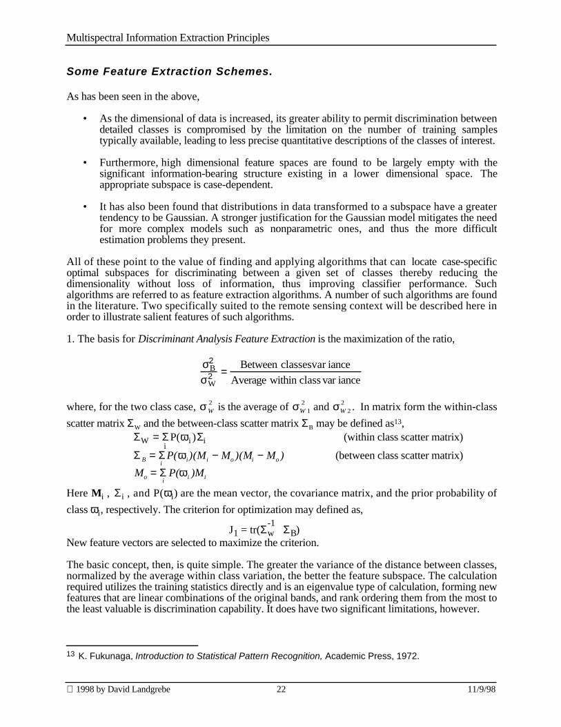
1. The basis for Discriminant Analysis Feature Extraction is the maximization of the ratio,
σB2
σW2 =
Between classesvar iance
Average within class var iance
where, for the two class case, σ W2 is the average of σW 1
2 and σW 22 . In matrix form the within-class
scatter matrix ΣW and the between-class scatter matrix ΣB may be defined as13,ΣW = Σ
iP(ω i )Σi (within class scatter matrix)
Σ B = Σi
P(ω i)(Mi − Mo )(Mi − Mo ) (between class scatter matrix)
Mo = Σi
P(ω i )Mi
Here Mi , Σ i , and P(ωi) are the mean vector, the covariance matrix, and the prior probability of
class ωi, respectively. The criterion for optimization may defined as,
J1 = tr(Σ-1w ΣB)
New feature vectors are selected to maximize the criterion.
The basic concept, then, is quite simple. The greater the variance of the distance between classes,normalized by the average within class variation, the better the feature subspace. The calculationrequired utilizes the training statistics directly and is an eigenvalue type of calculation, forming newfeatures that are linear combinations of the original bands, and rank ordering them from the most tothe least valuable is discrimination capability. It does have two significant limitations, however.
13 K. Fukunaga, Introduction to Statistical Pattern Recognition, Academic Press, 1972.

Multispectral Information Extraction Principles
1998 by David Landgrebe 23 11/9/98
First, it becomes ineffective if the classes involved have very little difference in mean values.Recall that classes, especially high dimensional ones, can be quite separable based on their secondorder statistics, i.e., their covariance matrices, alone. From the above ratio, it is apparent thatclasses with small difference in their means, but substantial separation due to their covariances,would not, by this means, lead to effective subspaces. A second limitation is that the method isonly guaranteed to provide reliable features up to one less than the number of classes. If one has aproblem that does not have a large number of classes, one will not have a very large subspace towork from. Still, the calculation involved is quite fast and very useful subspaces can be foundquickly in many cases.
2. A second feature extraction algorithm, called Decision Boundary Feature Extraction,14 does nothave the limitations just cited. It utilizes the training samples directly, rather than statistics derivedfrom them, to locate the decision boundary between the classes using a definition for discriminatelyinformative and discriminately redundant features. Then, using the effective portion of thatdecision boundary, an intrinsic dimensionality for the problem is determined and a transformationdefined which enables the calculation of the optimal features. The calculation produces not only thedesired new features, as linear combinations of the original ones, but it provides eigenvalues thatare a direct indication of how valuable each new feature will be. Since it works directly from thelocated decision boundary, it does not have the limitation of discriminant analysis feature extractionregarding class mean differences. However, it is quite a lengthy calculation, especially if thetraining set has many training samples. On the other hand, because it works directly with thetraining samples rather than statistics derived from them, it tends to be ineffective when the trainingset is small.
The value of high dimensional data on the one hand, but with the practical limitation of smalltraining sets on the other, means that compromises must be made in devising and using featureextraction algorithms, as in all other parts of the analysis process. Because of the quite broadvariation in the circumstances of data and user requirements, there is no single scheme that will beoptimal in all cases. The intent in describing the strengths and weaknesses of the above two featureextraction algorithms, is to illustrate that the analyst must be able to knowledgeable select the besttool for the circumstances.
Procedures for Information Extraction Problems.
It is appropriate at this point to coalesce the concepts described above into an effective procedurefor analyzing a data set. Though the specific steps needed varies with the scene, the data set and theclasses desired, the following diagram provides a general outline.
14 Chulhee Lee and David A. Landgrebe, "Feature Extraction Based On Decision Boundaries," IEEE
Transactions on Pattern Analysis and Machine Intelligence, Vol. 15, No. 4, April 1993, pp. 388-400.
Multispectral Information Extraction Principles
1998 by David Landgrebe 24 11/9/98
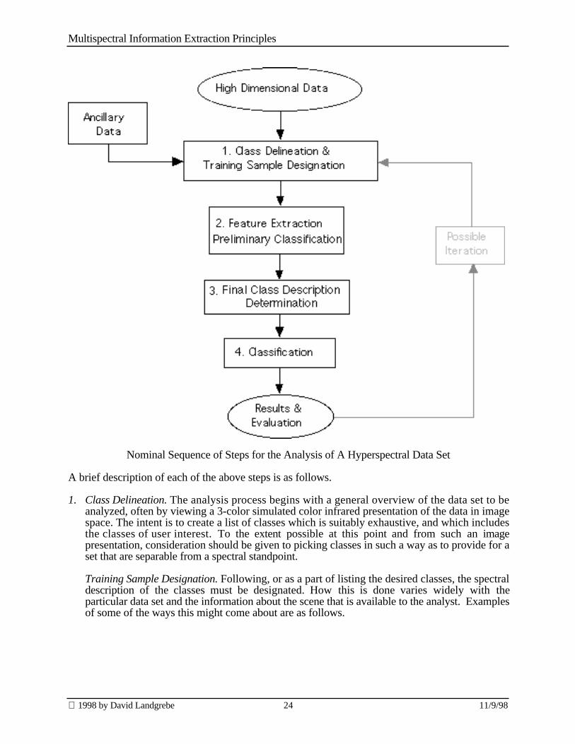
Nominal Sequence of Steps for the Analysis of A Hyperspectral Data Set
A brief description of each of the above steps is as follows.
1. Class Delineation. The analysis process begins with a general overview of the data set to beanalyzed, often by viewing a 3-color simulated color infrared presentation of the data in imagespace. The intent is to create a list of classes which is suitably exhaustive, and which includesthe classes of user interest. To the extent possible at this point and from such an imagepresentation, consideration should be given to picking classes in such a way as to provide for aset that are separable from a spectral standpoint.
Training Sample Designation. Following, or as a part of listing the desired classes, the spectraldescription of the classes must be designated. How this is done varies widely with theparticular data set and the information about the scene that is available to the analyst. Examplesof some of the ways this might come about are as follows.

Multispectral Information Extraction Principles
1998 by David Landgrebe 25 11/9/98
• Observations taken from a portion of the ground scene taken from the ground at the time ofthe data collection. See for example, [15] where this was done for a region-sized problemover an entire growing season to track a particular disease in a vegetative species.
• Observations from aerial photographs from which examples of each class can be labeled.See for example, [16] where again, this was done for a region-sized problem on a land usemapping problem.
• Conclusions that can be drawn directly from the image space, itself. See the exampleanalysis below, an urban mapping problem where the spatial resolution was great enoughto make objects of human interest recognizable in image space.
• Conclusions that can be drawn about individual pixels by observing a spectral spacerepresentation of a pixel. The use of “imaging spectroscopy” characteristics, where specificabsorption bands of individual molecules are used to identify specific minerals, are anexample of this. See [17] for an example.
2. Feature Extraction and Preliminary Classification. At this point one can expect to have trainingsets defined for each class, but they may be small. There would thus be value in eliminatingfeatures that are not effective for the particular set of classes at hand, so as to reduce thedimensionality without loss of information. A feature extraction algorithm would be used forthis purpose, followed by a preliminary classification. From the preliminary classification, onecan determine if the class list is suitably exhaustive, or if there have been classes of land coverof significant size that have been overlooked. One can also determine if the desired classes areadequately separable. If not, the classification can be used to increase the selection of trainingsamples, so that a more precise and detailed set of quantitative class descriptions aredetermined.
3. Final Class Description Determination. With the now augmented training set, in terms of eitheradditional classes having been defined or more samples labeled for the classes or both, any ofseveral steps may be taken to achieve the final class descriptions in terms of class statistics.• It may be appropriate to re-apply a feature extraction algorithm, given the improved class
descriptions. In this way, a more optimal subspace may be found.• The Statistics Enhancement algorithm may be applied. This algorithm is known to be
sensitive to outliers, and thus would not be expected to perform well until it is known thatthe list of classes is indeed exhaustive, as classes not previously identified would functionas outliers to the defined classes. The intended result of applying this algorithm at this pointis to increase the accuracy performance of the following classification and to improve thegeneralization capabilities of the classifier from the training areas to the rest of the data set.
• If the training set is still smaller than desirable relative to the number of features needed toachieve satisfactory performance, it might be appropriate to use the LOOC estimationscheme, which can function down to as few as three samples for a class.
15 MacDonald, R. B., M. E. Bauer, R. D. Allen, J. W. Clifton, J. D. Ericson, and D. A. Landgrebe, 1972,
"Results of the 1971 Corn Blight Watch Experiments," Proceedings of the Eighth InternationalSymposium on Remote Sensing of Environment, Vol. I. Environmental Research Institute ofMichigan, Ann Arbor, Michigan, pp. 157-190.
16 Swain, P. H. and S. M. Davis, Remote Sensing: The Quantitative Approach, McGraw-Hill, 1978, pp.309-314.
17 Hoffbeck, Joseph P. and David A. Landgrebe, “Classification of Remote Sensing Images having HighSpectral Resolution,” Remote Sensing of Environment, Vol. 57, No. 3, pp 119-126, September 1996.

Multispectral Information Extraction Principles
1998 by David Landgrebe 26 11/9/98
4. Classification. A final classification of adequatequality should be possible at this point, and evaluation ofit can proceed. However, if this is not the case, dependingon the nature of the further improvement needed, a returnto any of the above steps may be used.
Hyperspectral Analysis Example of Urban Data
The following is offered to illustrate this procedure. Thefigure to the left shows a color IR presentation of anairborne hyperspectral data flightline over the WashingtonDC Mall. The sensor system used in this case is known asHYDICE. It collects data in 210 bands in the 0.4 to 2.4µm region of the visible and infrared spectrum. This dataset contains 1208 scan lines with 307 pixels in each scanline. The data set totals approximately 150 Megabytes.With data of this complexity, one might expect a rathercomplex analysis process. However, following thescheme above, it is possible to achieve a quite simple andinexpensive analysis. The steps used and the time for thisanalysis needed on a personal computer costing less than$3000 are listed in the following table and are brieflydescribe below.
Operation CPU Time(sec.)
AnalystTime
Display Image 18Define Classes < 20 min.FeatureExtraction
12
Reformat 67InitialClassification
34
Inspect and Add2 Training Fields
≈ 5 min.
FinalClassification
33
Total 164 sec =2.7 min.
≈ 25 min.
Define Classes. A software application program calledMultiSpec, available to anyone at no cost from
http://dynamo.ecn.purdue.edu/~biehl/MultiSpec/ , is used. The first step is to present to the analyst a viewof the data set in image form so that training samples,examples of each class desired in the final thematic map,can be marked. A simulated color infrared photographform is convenient for this purpose; to do so, bands 60,27, and 17 are used in MultiSpec for the red, green, andblue colors, respectively. The result is shown at left. Theclasses desired in this case are, from the user’sstandpoint, quite simple. They are rooftops, streets,grass, and trees. Inspection of the image space
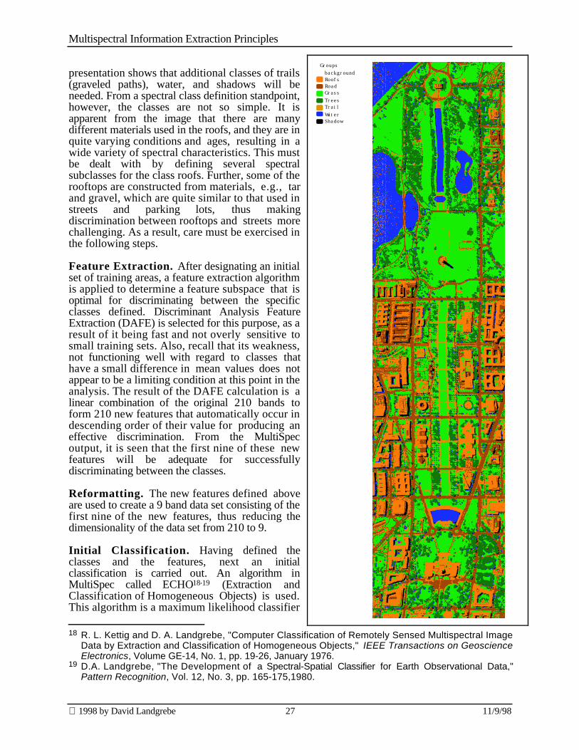
Multispectral Information Extraction Principles
1998 by David Landgrebe 27 11/9/98
presentation shows that additional classes of trails(graveled paths), water, and shadows will beneeded. From a spectral class definition standpoint,however, the classes are not so simple. It isapparent from the image that there are manydifferent materials used in the roofs, and they are inquite varying conditions and ages, resulting in awide variety of spectral characteristics. This mustbe dealt with by defining several spectralsubclasses for the class roofs. Further, some of therooftops are constructed from materials, e.g., tarand gravel, which are quite similar to that used instreets and parking lots, thus makingdiscrimination between rooftops and streets morechallenging. As a result, care must be exercised inthe following steps.
Feature Extraction. After designating an initialset of training areas, a feature extraction algorithmis applied to determine a feature subspace that isoptimal for discriminating between the specificclasses defined. Discriminant Analysis FeatureExtraction (DAFE) is selected for this purpose, as aresult of it being fast and not overly sensitive tosmall training sets. Also, recall that its weakness,not functioning well with regard to classes thathave a small difference in mean values does notappear to be a limiting condition at this point in theanalysis. The result of the DAFE calculation is alinear combination of the original 210 bands toform 210 new features that automatically occur indescending order of their value for producing aneffective discrimination. From the MultiSpecoutput, it is seen that the first nine of these newfeatures will be adequate for successfullydiscriminating between the classes.
Reformatting. The new features defined aboveare used to create a 9 band data set consisting of thefirst nine of the new features, thus reducing thedimensionality of the data set from 210 to 9.
Initial Classification. Having defined theclasses and the features, next an initialclassification is carried out. An algorithm inMultiSpec called ECHO18,19 (Extraction andClassification of Homogeneous Objects) is used.This algorithm is a maximum likelihood classifier
18 R. L. Kettig and D. A. Landgrebe, "Computer Classification of Remotely Sensed Multispectral Image
Data by Extraction and Classification of Homogeneous Objects," IEEE Transactions on GeoscienceElectronics, Volume GE-14, No. 1, pp. 19-26, January 1976.
19 D.A. Landgrebe, "The Development of a Spectral-Spatial Classifier for Earth Observational Data,"Pattern Recognition, Vol. 12, No. 3, pp. 165-175,1980.
backgroundRoofsRoadGrassTreesTrailWaterShadow
Groups
Multispectral Information Extraction Principles
1998 by David Landgrebe 28 11/9/98
that first segments the scene into spectrally homogeneous objects. It then classifies the objectsutilizing both first and second order statistics, thus taking advantage of spatial characteristics of thescene, and doing so in a multivariate sense.
Finalize Training. An inspection of the initial classification result indicates that someimprovement in the set of classes is called for. To do so, two additional training fields wereselected and added to the training set.
Final Classification. The data were again classified using ECHO and the new training set. Theresult is shown above. An examination of this result shows that it provides a reasonably accuratethematic presentation of the scene. If further refinement of the result would be desired, it might bedesirable to increase the size of the training sets by choosing additional pixels representative ofeach of the classes. It might also be desirable to apply the Statistics Enhancement scheme. Anadditional possibility might be to use the Decision Boundary Feature Extraction (DBFE) algorithmto the original data using the augmented training sets. Recall that DBFE does not have the limitationof DAFE with regard to classes that have nearly equal mean vectors, but it does require largernumbers of training samples to deliver good performance.
Concluding Remarks
Advances made in sensor system technology in recent years have effectively removed one of themost significant barriers to improved performance in multispectral remote sensing systems, namelythe limited spectral dimensionality of these systems previously. The much increased dimensionalitymakes possible substantially more accurate and more detailed discriminations. However, the priceto be paid for this improvement is the need to be able to more precisely define quantitatively theclasses to be discriminated, as the above material makes clear.
There are, of course, many valid ways to approach the analysis of multispectral data, and a greatrange of user needs, from the mapping of simple classes to a desire to discriminate between classeswith only very subtle differences. In exploring the nature of hyperspectral data, we have focusedupon methods for the most challenging cases, in order to probe the limits of the potential of suchdata. To provide a simple explanation of the potential of high dimensional data, consider the caseof hyperspectral data of 100 bands, gathered with a signal-to-noise ratio high enough to justify aten bit data system. In this case, there would be 210 = 1024 possible values in each band, and atotal of 1024100 ≈ 10 300 possible different discrete locations in the feature space. This is a hugenumber, so large that even for a data set containing 106 pixels, the probability of any two pixelslanding in the same feature space cell is vanishingly small. This means that, before evenconsidering the cause/effect relationship between the physical characteristics of pixel areas on theground and their spectral response or atmospheric or other such effects, one can conclude that,since there is no overlap of pixels in such a feature space, anything is theoretically separable fromanything. The problem is that to approach this possibility, one must be able to locate a decisionboundary between pixels of different desired classes correctly and precisely. As the dimensionalityand therefore the volume available in such feature spaces grows, the estimation precision mustgrow as well and very rapidly so.
In this chapter, we studied the characteristics of high dimensional spaces quantitatively in order tounderstand, document, and make credible such potential. The results suggest a fundamental shift inthe analysis paradigm from that common today. Much current literature on multispectral analysissuggests studying cause/effect relationships of spectral responses with the intent to using thatknowledge directly to achieve classification. Implied in this is the thought that, documenting thespectral response of various materials will allow the analysis of later spectral data sets based uponsuch documented responses.

Multispectral Information Extraction Principles
1998 by David Landgrebe 29 11/9/98
From a purely scientific standpoint, such work is certainly valuable, for it increases theunderstanding of the interaction of electromagnetic energy with scene materials. However, naturalscenes are not only very complex but very dynamic as well. Thus the spectral response of a givenmaterial is not very stable over time and place. Increasing the dimensionality of such data, whileenhancing the potential for discrimination, does not materially change this stability problem. A nowcommon line of approach to solving this dilemma has been to “correct” the data, i.e. to attempt toadjust the data for the various factors that have changed from one observation time and place toanother. Such factors include the atmospheric effects, the illumination and view angle effects dueto the non-Lambertian characteristics of most scene materials, changes in hemispheric illumination,the adjacency effect, and many more. This has lead to very extended studies of some very dauntingproblems.
After many years of study of the effects of the atmosphere, for example, about the best that isclaimed for atmospheric adjustment is an accuracy of 2 to 5%, a level that does not favorablycompare with the 0.1% measurement level implied by 10 bit data common today. Thus it may notbe helpful nor perhaps even wise to use such calculations directly in the classification of data. Atthe very least, it introduces a complex step into the analysis process, one that may have littlepositive effect on the accuracy achieved in the generation of a thematic map. Further, it is only oneof a number of such adjustments that would be necessary to reconcile conditions between datacollected at different times or places.
The field of wireless communication faced a similar problem in its development many years ago. Inthat case, rather than attempting to adjust for or subtract out the many sources of interference (e.g.,noise generated in the atmosphere, by other competing signal sources, etc.) and distortion (e.g.,multipath, fading, etc.) and the like, the approach was initially to model the corrupting influences,as well as the signals desired, and then to construct optimal detection procedures that discriminatebetween them. The success of this approach, obviously after much further development, is seen inthe clarity of modern digital cellular phone messages through complex urban environments, forexample, or in the communication possible from planetary and deep space probes using very lowtransmitter power.
Spectra collected at another time or place can certainly represent useful information, and there areusually many other pieces of information, some quantitative, some subjective, that are availableabout a scene when one begins an analysis process. Rather than attempting to use such spectracollected at another time, place, or with another instrument directly in the analysis process, a moreviable approach would seem to be to use the knowledge gained from such measurements togetherwith other ancillary information to label examples of classes of interest in the data set to beanalyzed. In this way, a suitable collection of spectra, representing the range of conditions andcircumstances existing in the current data set, could be constructed that would indeed define theclasses of interest to adequate precision.
Using such information to label “training samples,” rather than attempting to use it directly in theanalysis process, means that the analysis can take place on the original, “uncorrected” data. Thishas several advantages. First of all, it greatly reduces the amount and complexity of the processingthat must be done to the data, since it does not involve further calibration of the data, removing theatmospheric and other effects, conversion from radiance to reflectance, and other suchadjustments. If any of these processes need to be carried out to label training samples, it wouldinvolve such processing on a much smaller quantity of data. However, perhaps more importantly,use of this approach means that any unsuspected corrupting influences of such processing, whichnecessarily will always be imperfect, would be avoided. Since the analyst has no way to tell if suchprocessing, which seems on the face of it, so logical, actually helps or hinders, a cleaner, simpleranalysis process results. The secret, then, is in the adequacy of the precision and detail by whichthe user quantitatively specifies the classes of interest, and doing so in the data set to be analyzed

Multispectral Information Extraction Principles
1998 by David Landgrebe 30 11/9/98
by labeling an adequate number of training samples. It is basically the inverse of the computeruser’s mantra, “Garbage in, Garbage out,” namely, precise and careful specification of what isdesired put into the analysis process can lead to precise and accurate output.