
INFORMATION ENRICHMENT FOR QUALITY RECOMMENDER SYSTEMS · Recommender systems have been an active...
247
INFORMATION ENRICHMENT FOR QUALITY RECOMMENDER SYSTEMS Li-Tung Weng (B.Sc. (Hons)) A Dissertation Submitted in Fulfil of the Requirements for the Degree of Doctor of Philosophy Faculty of Information Technology Queensland University of Technology Brisbane, Australia November 2008
Transcript of INFORMATION ENRICHMENT FOR QUALITY RECOMMENDER SYSTEMS · Recommender systems have been an active...

INFORMATION ENRICHMENT FOR
QUALITY RECOMMENDER SYSTEMS
Li-Tung Weng (B.Sc. (Hons))
A Dissertation
Submitted in Fulfil of the Requirements for the Degree of
Doctor of Philosophy
Faculty of Information Technology
Queensland University of Technology
Brisbane, Australia
November 2008


Page i
Keywords
Collaborative Filtering, Cold-Start Problem, Distributed Systems, Ecommerce, Product
Taxonomy, Recommendation Novelty, Recommender Systems

Page ii
Abstract
The explosive growth of the World-Wide-Web and the emergence of ecommerce
are the major two factors that have led to the development of recommender systems
(Resnick and Varian, 1997). The main task of recommender systems is to learn from
users and recommend items (e.g. information, products or books) that match the users’
personal preferences.
Recommender systems have been an active research area for more than a decade.
Many different techniques and systems with distinct strengths have been developed to
generate better quality recommendations. One of the main factors that affect
recommenders’ recommendation quality is the amount of information resources that are
available to the recommenders. The main feature of the recommender systems is their
ability to make personalised recommendations for different individuals. However, for
many ecommerce sites, it is difficult for them to obtain sufficient knowledge about their
users. Hence, the recommendations they provided to their users are often poor and not
personalised. This information insufficiency problem is commonly referred to as the
cold-start problem.
Most existing research on recommender systems focus on developing techniques
to better utilise the available information resources to achieve better recommendation
quality. However, while the amount of available data and information remains
insufficient, these techniques can only provide limited improvements to the overall
recommendation quality.
In this thesis, a novel and intuitive approach towards improving recommendation
quality and alleviating the cold-start problem is attempted. This approach is enriching the

Page iii
information resources. It can be easily observed that when there is sufficient information
and knowledge base to support recommendation making, even the simplest
recommender systems can outperform the sophisticated ones with limited information
resources. Two possible strategies are suggested in this thesis to achieve the proposed
information enrichment for recommenders:
The first strategy suggests that information resources can be enriched by
considering other information or data facets. Specifically, a taxonomy-based
recommender, Hybrid Taxonomy Recommender (HTR), is presented in this
thesis. HTR exploits the relationship between users’ taxonomic preferences
and item preferences from the combination of the widely available product
taxonomic information and the existing user rating data, and it then utilises
this taxonomic preference to item preference relation to generate high
quality recommendations.
The second strategy suggests that information resources can be enriched
simply by obtaining information resources from other parties. In this thesis,
a distributed recommender framework, Ecommerce-oriented Distributed
Recommender System (EDRS), is proposed. The proposed EDRS allows
multiple recommenders from different parties (i.e. organisations or
ecommerce sites) to share recommendations and information resources with
each other in order to improve their recommendation quality.
Based on the results obtained from the experiments conducted in this thesis, the
proposed systems and techniques have achieved great improvement in both making
quality recommendations and alleviating the cold-start problem.

Page iv
Acknowledgements
Thanks to God for giving me such a great opportunity to conduct my PhD
research, and the past four year’s time in my career as a research student was truly joyful
and unforgettable. If I have ever achieved anything in my life, they are not from me but
from God.
I am indebted to a great number of people who kindly offered advice,
encouragement, inspiration and friendship through my time at QUT. Firstly, I would like
to express my utmost gratitude to my principal supervisor and mentor Dr. Yue Xu for
her guidance, her support, for the opportunities she has provided me and for the
invaluable insight she offered me. I am also thankful to my associate supervisors, Dr.
Yuefeng Li and Dr. Richi Nayak, they have provided instrumental inputs and guidance
for my research.
In countless ways, I have received support and love from my family. I would like
to take this opportunity to thank them for all the love, encouragement and wonderful
moments they shared with me over the years. To my mum, for her endless love and
caring, to whom I hope I have given back a fraction of what I have received. To my
brother, Samuel, for providing me support and entertainment. To my father, for his
accompany in my childhood. Finally, I would like to thank my friends and church family,
for all of their supports, prayers and encouragement during my life in Australia.

Page v
Table of Contents
Keywords ................................................................................................................................................. i
Abstract .................................................................................................................................................. ii
Acknowledgements ................................................................................................................................ iv
Acknowledgements ................................................................................................................................ iv
Table of Contents .................................................................................................................................... v
List of Figures ...................................................................................................................................... vii
List of Tables ......................................................................................................................................... ix
Statement of Original Authorship ........................................................................................................... x
1 INTRODUCTION ............................................................................................................................. 1
1.1 Problem Statement ....................................................................................................................... 5
1.2 Contributions ............................................................................................................................... 6
1.3 Research Methodology ................................................................................................................ 8
1.4 Thesis Outline .............................................................................................................................. 9
2 LITERATURE REVIEW ............................................................................................................... 13
2.1 Recommender Systems .............................................................................................................. 13 2.1.1 Content-Based Filtering .................................................................................................. 13 2.1.2 Collaborative Filtering .................................................................................................... 16 2.1.2.1 Item-based Collaborative Filtering ................................................................................. 20 2.1.3 Demographic Filtering .................................................................................................... 21 2.1.4 Hybrid Techniques ......................................................................................................... 22
2.2 Taxonomy-based recommender systems ................................................................................... 26
2.3 Distributed recommender systems ............................................................................................. 27
2.4 Evaluating Recommender Systems ............................................................................................ 33 2.4.1 Accuracy Metrics ............................................................................................................ 36 2.4.1.1 Predictive Accuracy Metrics ........................................................................................... 36 2.4.1.2 Classification Accuracy Metrics ..................................................................................... 38 2.4.2 Beyond Accuracy ........................................................................................................... 40
2.5 Implications ............................................................................................................................... 42
3 MAKING RECOMMENDATIONS WITH ITEM TAXONOMY ............................................. 45
3.1 Related work .............................................................................................................................. 48
3.2 Proposed approach ..................................................................................................................... 49 3.2.1 Notation .......................................................................................................................... 50 3.2.2 Item Preferences based User Clusters ............................................................................. 55 3.2.3 Item Preferences - Taxonomic Preference Relation ....................................................... 58 3.2.4 Extraction of User’s Taxonomic Preferences ................................................................. 59 3.2.4.1 Personal Taxonomic Preference ..................................................................................... 59 3.2.4.2 Cluster Taxonomic Preference ........................................................................................ 66 3.2.4.3 Merge Personal and Cluster Taxonomic Preferences ..................................................... 68 3.2.5 Hybrid Taxonomy Recommender .................................................................................. 69 3.2.6 Cold-Start Proof Hybrid Taxonomy Recommender ....................................................... 75
3.3 Experiments and evaluation ....................................................................................................... 81 3.3.1 Data Acquisition ............................................................................................................. 82 3.3.2 Verification for Item Preferences - Taxonomic Preference Relation .............................. 82 3.3.3 System Evaluations ......................................................................................................... 86

Page vi
3.3.3.1 Experiment Framework .................................................................................................. 86 3.3.3.2 Parameterisation ............................................................................................................. 89 3.3.3.3 Evaluation Metrics .......................................................................................................... 91 3.3.3.4 Experimental Results ...................................................................................................... 93
3.4 Chapter Summary .................................................................................................................... 105
4 DISTRIBUTED RECOMMENDATION MAKING ................................................................... 107
4.1 Related work ............................................................................................................................ 108
4.2 ECommerce-oriented Distributed Recommender .................................................................... 111 4.2.1 General Interaction Protocol ......................................................................................... 119
4.3 Peer Profiling and Selection .................................................................................................... 125 4.3.1 System Formalisation for EDRS .................................................................................. 126 4.3.2 User Clustering ............................................................................................................. 127 4.3.3 Recommender Peer Profiling ........................................................................................ 128 4.3.4 Recommender Peer Selection ....................................................................................... 132 4.3.4.1 Gittins Indices ............................................................................................................... 132 4.3.4.2 Selection Strategy for EDRS ........................................................................................ 137 4.3.4.3 An Example .................................................................................................................. 138
4.4 Recommendation Merge .......................................................................................................... 140
4.5 Experiments and Evaluation .................................................................................................... 144 4.5.1 Data Acquisition ........................................................................................................... 145 4.5.2 Experiment Setup ......................................................................................................... 146 4.5.2.1 Constructing the Recommender Peers .......................................................................... 146 4.5.2.2 Evaluation Metrics ........................................................................................................ 151 4.5.2.3 Benchmarks for the Peer Profiling and Selection Strategy ........................................... 152 4.5.2.4 Simulating the User Feedbacks .................................................................................... 154 4.5.3 Experimental Results .................................................................................................... 155
4.6 Chapter Summary .................................................................................................................... 159
5 CONCLUSIONS ............................................................................................................................ 160
5.1 Contributions ........................................................................................................................... 161
5.2 Future work .............................................................................................................................. 163
APPENDIX A: STATISTICAL ATTRIBUTE DISTANCE ......................................................... 165
APPENDIX B: HYBRID PARITITIONAL CLUSTERING ........................................................ 178
APPENDIX C: RELATIVE DISTANCE FILTERING ................................................................ 207
BIBLIOGRAPHY ............................................................................................................................. 223

Page vii
List of Figures
Figure 1.1. The proposed research method for this thesis. ...................................................................... 8
Figure 3.1: An example fragment of item taxonomy extracted from Amazon.com. ............................. 54
Figure 3.2: An example list of items with their taxonomic descriptors. ................................................ 55
Figure 3.3: Reduce neighbourhood searching space with clustering .................................................... 56
Figure 3.4. The impact of different values on 2 ( 0.28) ........................................................... 73
Figure 3.5. The impact of different values on 2 .............................................................................. 73
Figure 3.6. Recommender evaluation with precision metric ................................................................. 95
Figure 3.7. Recommender evaluation with recall metric ....................................................................... 96
Figure 3.8. Recommender evaluation with F1 metric ........................................................................... 96
Figure 3.9. Computation efficiency results for different recommenders (average seconds per recommendation) .......................................................................................................................... 97
Figure 3.10. F1 results for HTR with different 1 and configurations. ........................................... 100
Figure 3.11. F1 results for HTR with different configurations ( 1 0.2) ...................................... 101
Figure 3.12. F1 results for HTR with different 1 configurations ( 0.8) ...................................... 101
Figure 3.13. Recommender evaluation under cold-start situations with precision metrics ................. 104
Figure 3.14. Recommender evaluation under cold-start situations with recall metrics ....................... 104
Figure 3.15. Recommender evaluation under cold-start situations with F1 metrics ........................... 105
Figure 3.16. Computation efficiencies for CSHTR and TPR .............................................................. 105
Figure 4.1. Classical centralised recommender system ....................................................................... 114
Figure 4.2. Standard distributed recommender system ....................................................................... 116
Figure 4.3. Proposed distributed recommender system ....................................................................... 119
Figure 4.4. High level interaction overview for EDRS (based on contract net protocol) .................... 121
Figure 4.5. The relation between and Gittins Indices when 0.9 ............................................... 135
Figure 4.6. Precision results for different recommendation settings ................................................... 158
Figure 4.7. Recall results for different recommendation settings ........................................................ 158
Figure 4.8. F1 results for different recommendation settings .............................................................. 159
Figure A.1. A graph for demonstrating the concept of the standard similarity measures ................... 171
Figure A.2. A graph for demonstrating the concept of the proposed SAD technique ......................... 172
Figure A.3. Comparison between IUF and SAD with training sets of different sizes ......................... 177
Figure B.1. The three major consecutive phases of the proposed HPC technique .............................. 182
Figure B.2. A possible dataset with a single cluster ............................................................................ 192
Figure B.3. An example of centroid estimation based on Equation (B.10) ......................................... 192
Figure B.4. A possible dataset containing multiple clusters ................................................................ 193
Figure B.5. Centroids estimation for the complex dataset with multiple clusters based on Equation (B.10).......................................................................................................................................... 194

Page viii
Figure B.6. An example of virtual boundaries for each of the clusters in the dataset ......................... 194
Figure B.7. An example of cluster centroids estimation process ........................................................ 197
Figure B.8. Partition quality comparison with different k-means settings .......................................... 200
Figure B.9. Computation time comparison with different k-means settings ....................................... 201
Figure B.10. Intra-cluster similarity of the resulting cluster partitions ............................................... 206
Figure B.11. Inter-cluster distance of the resulting cluster partitions ................................................. 206
Figure B.12. overall quality of the resulting cluster partitions ............................................................ 206
Figure C.1. A simple example of the suggested geometrical implication ........................................... 210
Figure C.2. An example of projected user set ..................................................................................... 211
Figure C.3. Estimated searching space with three reference users ...................................................... 213
Figure C.4. An example structure of the RDF searching cache .......................................................... 216
Figure C.5. Precision Results for different TPR versions ................................................................... 221
Figure C.6. Recall Results for different TPR versions ........................................................................ 221
Figure C.7. Average recommendation time for different TPR versions .............................................. 222

Page ix
List of Tables
Table 3.1. The effect of user clustering on taxonomy information gain ............................................... 86
Table 3.2. Information for the two different testing datasets ................................................................ 93
Table 4.1. High level aspect differences among recommender system paradigms ............................. 118
Table 4.2. The Gittins indices table for 0.9 ................................................................................. 136
Table 4.3. Performance histories for four recommender peers ........................................................... 139
Table 4.4. Allocation details for the training and testing user sets ...................................................... 149
Table 4.5. Dataset allocation details for the four recommender peers ................................................ 150

Page x
Statement of Original Authorship
The work contained in this thesis has not been previously submitted to meet
requirements for an award at this or any other higher education institution. To the best of
my knowledge and belief, the thesis contains no material previously published or written
by another person except where due reference is made.
Signature: _________________________
Date: _________________________

Page 1
Chapter 1
1Introduction
The receipt of undesirable or non-relevant information is generally referred to as
information overload (Schafer et al., 2000, Yang et al., 2003). Nowadays, due to the
advancement of internet technology and the World Wide Web (WWW), the issue of
information overload has become increasingly serious. Significant efforts in research are
being invested in building support tools that ensure the right information is delivered to
the right people at the right time. Recommender systems are one of the recent inventions
aiming to help humans deal with this information explosion by giving information
recommendations according to their personal information needs (Linden et al., 2003,
Sarwar et al., 2000b, Schafer et al., 2000). Recommender systems have been applied to
many application areas, including the domain of ecommerce, in which a recommender
system is used to suggest products to customers, and these product suggestions are often
tailored to individual customers’ interests (Linden et al., 2003). Recommender systems
stand out from other information filtering applications in their ability to provide
personalised information recommendations. For example, while standard search engines
are very likely to generate identical search results for users with identical search queries,
recommender systems are able to generate recommendations that are personalised based
on different users’ personal interests (or past behaviours, etc.) even if the users have
identical search queries.
In order to generate personalised recommendations, recommender systems need
to have users’ personal data available. Such personal data includes user demographic
information, user browsing histories, shopping histories, item ratings and user comments.

Page 2
Unfortunately, users’ personal data is difficult to obtain, especially when that data
directly reveal users’ personal interests (e.g. users’ explicit item ratings or comments)
(Park et al., 2006, Schein et al., 2002). Specifically, the situation where a recommender
system has insufficient information resources (e.g. users’ personal data) to generate
quality recommendations is commonly referred to as the cold-start problem (Schein et al.,
2002, Park et al., 2006).
While many of the real world recommender systems suffer from having
insufficient personal data to generate quality personalised recommendations, many
recommender related studies strive to exploit new strategies to better utilise the limited
amount of personal data and information resources to produce better recommendations
(Adomavicius et al., 2005, Badrul et al., 2001, Basu et al., 1998, Deshpande and Karypis,
2004, Goldberg et al., 1992, Jerome and Derek, 2004, Jun et al., 2006). The following
are the main existing strategies for tackling the cold-start problem and improving
recommendation quality:
Developing more sophisticated algorithms to achieve better utilisation of the
limited available information resources (Breese et al., 1998, Montaner et al.,
2003). For example, there are many techniques from other research domains
being applied to recommender systems, such as Bayesian network (Breese et
al., 1998), Neural network (Schafer et al., 2000), and Support Vector
Machine (SVM) (Min and Han, 2005). While some of these advanced
techniques were reported to have achieved better performance, given limited
information resource, the amount of the improvements achieved is often
limited as well.
Hybridising with other techniques that are less dependent on user personal
data (Balabanović and Shoham, 1997, Basu et al., 1998, Burke, 2002). For

Page 3
example, recommenders that are based on users’ personal data can be
combined with standard information filtering techniques, hence, whenever
the recommenders have insufficient personal data to make recommendations
they can use the information filtering techniques as complements to make
recommendations in the case of a cold-start situation. However, such
strategy often risks producing less personalised recommendations.
Even though efforts have been made to improve recommendation quality and
alleviate cold-start problem, no satisfactory solutions have been found so far and the
cold-start problem is still a challenging research problem. This thesis attempts to explore
new strategies to tackle the recommendation making problem – improving
recommendations through information enrichment. As stated earlier, most studies on
recommender systems have been focused on better utilising existing available
information resources, however, very few studies realise that it is also desirable to
increase effectively the amount of information resources available for making
recommendations. In this research, the importance of information enrichment for
recommender systems is highlighted. The objective of this research is to develop
effective strategies to achieve the information enrichment for the recommenders, and
then demonstrate that recommender systems’ performance can be effectively improved
when the available information resources are enriched. Concretely, two novel
recommendation strategies based on the notion of information enrichment are proposed
in this thesis. They are Hybrid Taxonomy Recommender (HTR) and Ecommerce-
oriented Distributed Recommender System (EDRS).
The HTR utilises item taxonomy information with user rating data to make
quality recommendations. One of its major contributions is that it demonstrated the
possibility of integrating user unrelated data (e.g. item taxonomy, item contents, etc.) and

Page 4
users’ personal data (e.g. users’ item ratings and comments) into a useful knowledgebase
that represents users’ interests at a deeper depth. Specifically, HTR extracts the
relationship between users’ item interests and taxonomy interests from the given item
taxonomy information and user rating data, and utilises this relationship to make quality
recommendations. It is shown in our experiment that HTR is able to generate high
quality personal recommendations even under severe cold-start situations. To the best of
our knowledge, there is no similar research that explores the relationship between users’
item preferences and item taxonomic preferences, and exploits this relationship to
produce better recommendations.
The EDRS is a distributed framework that allows multiple recommenders from
different parties (i.e. organisations and ecommerce sites) to cooperate with each other as
well as sharing their information resources and recommendations. While many existing
research on recommender systems focuses on exploring new techniques to better utilise
available information resources, this thesis suggests that if the available information
resources can be enriched, recommenders’ recommendation quality would also be
improved. The cold-start problem would, therefore, be alleviated as well. The idea
behind the proposed EDRS is that instead of improving a recommender’s underlying
algorithm to make better recommendations, the recommender can cooperate with
recommenders from other parties to obtain additional information resources and
recommendations to enrich its available information resources and improve its
recommendation quality. In order to allow the recommenders within the proposed EDRS
to effectively cooperate and interact with each other, a novel recommender peer profiling
and selection strategy is also presented in this thesis. It allows recommenders to learn
from each other and select the most appropriate recommenders to assist in making
recommendations. It is shown in our experiment that by allowing recommenders to

Page 5
cooperate and share their recommendations, their recommendation quality can be
drastically improved. To the best of our knowledge, there is no concept similar to the
proposed EDRS framework in any other research.
Besides the above-mentioned two major contributions (i.e. HTR and EDRS),
three new recommender-related techniques are also developed during this thesis, and
they are Statistical Attribute Distance (SAD), Hybrid Partitional Clustering (HPC), and
Relative Distance Filtering (RDF). These three additional contributions are generic level
techniques designed for improving common recommenders’ recommendation accuracy
and efficiency, and they have been utilised in the development of this thesis. However,
because these three additional studies are not strongly related to the overall theme of this
thesis (i.e. information enrichment), they are not included in the main body of the thesis.
Instead, they are appended as the appendices of this thesis.
To summarise, while many existing studies on recommender systems are about
exploring new techniques to better utilise available information resources, the main
objective of this thesis is to exploit new data resources (i.e. item taxonomy data) and new
system structure (i.e., distributed framework) to achieve information enrichment for
improving recommendation quality and coping with the cold-start problem.
1.1 PROBLEM STATEMENT
Most research on the recommender system community has focused on
developing algorithms to improve recommenders’ recommendation quality, especially in
the situation where only limited information resources are available (i.e. to cope with the
cold-start problem). Majority of the recommender related studies focus on developing
approaches to better utilise the limited available information resources to form better
recommendations. However, given insufficient information resources, the amount of

Page 6
improvements that can be gained from these techniques is very limited. Hence,
improving recommendation quality and alleviating the cold-start problem are still
unresolved problems.
While it is difficult to produce quality recommendations with limited information
resources, it can be easily observed that, if the information resources can be enriched, the
recommendation quality can be drastically improved. The main research problem
involved in this thesis is to explore and develop strategies to achieve the information
enrichment in order to improve recommendation quality and tackle the cold-start
problem.
1.2 CONTRIBUTIONS
This thesis proposes to improve recommenders’ recommendation quality and
tackle the cold-start problem by enriching recommenders’ available information
resources. Two systems are proposed in this thesis, and each of them uses a different
strategy to achieve information enrichment for improving recommendation quality. The
first system, Hybrid Taxonomy Recommender (HTR), utilises the commonly available
product taxonomy information in conjunction with users’ rating data to make quality
recommendations, and it features in strong resistance to cold-start problems. The second
system, Ecommerce-oriented Distributed Recommender System (EDRS), allows
recommenders from different parties to share their information resources and
recommendations with each other and make recommendations cooperatively. EDRS
allows recommenders with insufficient information resources to gain drastic
improvements in their recommendations by providing them with help from other
recommenders. The summarised contributions are briefed as follows:

Page 7
A novel recommender system, HTR, is proposed. It utilises the new
information resource (i.e. product taxonomy information) for making quality
recommendations.
A novel distributed recommender system framework, EDRS, is proposed. It
allows recommender from different parties to share their information
resources and recommendations in a distributed fashion.
A novel recommender peer profiling and selection strategy is proposed to
allow recommenders to learn from each other and achieve more efficient
and effective interactions within EDRS. Overall, by adopting the proposed
peer profiling and selection strategy, the performance of the proposed EDRS
can be effectively improved.
Experimental evaluations are made and the results prove the feasibility and
effectiveness of the proposed HTR and EDRS. Moreover, the experimental
results obtained also suggest that the notion of information enrichment in
recommender systems is significant.
An advanced similarity measure, Statistical Attribute Distance (SAD),
which allows recommenders to more objectively compute the similarities
among user profiles.
A novel clustering method, Hybrid Partitional Clustering (HPC), is proposed.
It allows recommenders to generate efficiently and effectively user or item
clusters. HPC features in its simplicity to use and the ability to update the
clustering results incrementally in accordance to the dataset changes.
A novel neighbourhood formation technique, Relative Distance Filtering
(RDF), is proposed. It allows recommenders to locate efficiently a target
user’s neighbourhood from a large dataset. RDF features in its accuracy,

Page 8
computation efficiency and memory compactness in comparison to other
existing neighbourhood formation techniques.
1.3 RESEARCH METHODOLOGY
Various research approaches have been used in the recommender system field,
and some of these methods include survey, case studies, prototyping and experimenting
(Sarwar et al., 2000a, Herlocker et al., 2004, Schafer et al., 2000). As the research is
considered to focus on the development of new systems or techniques in the
recommender system, and the soundness of these systems, techniques or proposed
strategies have to be supported by the results from the experimentations and evaluations.
Hence, the experimenting approach integrated with the standard information system
research cycle is chosen as the proposed research method. The process of the research
approach used in this research is illustrated in Figure 1.1.
Figure 1.1. The proposed research method for this thesis.

Page 9
1.4 THESIS OUTLINE
The rest of this thesis is summarised as follows:
Chapter 2: This chapter is a literature review of related recommender
techniques, including both conventional and state of the art recommender
systems. In particular, existing studies on taxonomy-based recommenders
and distributed recommenders are reviewed in depth. It pinpoints the current
research on recommender systems and identifies the gap between the
existing recommender studies.
Chapter 3: This chapter presents the proposed Hybrid Taxonomy
Recommender (HTR) and the techniques involved for constructing
knowledgebase from both the taxonomy information and user rating data.
The experimental process involved for evaluating the system and the
experimental results obtained are detailed in this chapter. The relevant
publications about this chapter are:
o Weng, L.T., Xu, Y., Li, Y., and Nayak, R., ‘Improve Recommendation
Quality with Item Taxonomic Information’, Lecture Notes in Business
Information Processing, 2008.
o Weng, L.T., Xu, Y., Li, Y., and Nayak, R., ‘Web Information
Recommendation Making based on Item Taxonomy’, proceedings
of 10th International Conference on Enterprise Information Systems
(ICEIS2008), 20-28, Barcelona, Spain, June. 2008.
(This publication received the best paper award from the
ICEIS2008).
o Weng, L.T., Xu, Y., Li, Y., and Nayak, R., ‘Exploiting Item Taxonomy
for Solving Cold-start Problem in Recommendation Making’, 20th IEEE

Page 10
International Conference on Tools with Artificial Intelligence
(ICTAI2008) , Dayton, Ohio, USA, Nov. 2008.
o Weng, L.T., Xu, Y., Li, Y., and Nayak, R., ‘Improving Recommendation
Novelty Based on Topic Taxonomy’, proceedings of Workshop on Web
Personalization and Recommender Systems (WPRS2007), conjunction
with the 2007 IEEE/WIC/ACM International Conferences on Web
Intelligence and Intelligent Agent, 115-118, Silicon Valley, USA, Nov.
2007.
Chapter 4: This chapter presents the proposed Ecommerce-oriented
Distributed Recommender System (EDRS) and a novel recommender peer
profiling and selection technique that is designed for facilitating the overall
performance of the proposed EDRS. The experimental process involved for
evaluating the system and the experimental results obtained are detailed in
this chapter. The relevant publications about this chapter are:
o Weng, L.T., Xu, Y., Li, Y., and Nayak, R., ‘Distributed Recommender
Profiling and Selection with Gittins Indices’, proceedings
of IEEE/WIC/ACM International Conference on Web Intelligence
(WI2006), 290-293, Hong Kong, China. 2006.
o Weng, L.T., Xu, Y., Li, Y., and Nayak, R., ‘A Fair Peer Selection
Algorithm for an Ecommerce-Oriented Distributed Recommender
System’, accepted by the 4th International Conference on Active Media
Technology, 31-37, Brisbane, Australia, 2006.
o Weng, L.T., Xu, Y., Li, Y., ‘Framework for Ecommerce Oriented
Recommendation Systems’, proceedings of the 4th International

Page 11
Conference on Active Media Technology (AMT05), 19-21 May, 2005,
Japan.
Chapter 5: This chapter concludes this thesis and draws the direction for
future work.
Appendices: In the appendices of this thesis, three novel neighbourhood
formation related techniques designed for helping recommenders to achieve
better recommendation quality and computation efficiency are included. The
relevant publications are:
o Weng, L.T., Xu, Y., Li, Y., and Nayak, R., ‘An Efficient Neighbourhood
Estimation Technique for Making Recommendations’, Lecture Notes in
Business Information Processing, 2008. (Accepted)
o Weng, L.T., Xu, Y., Li, Y., and Nayak, R., ‘Efficient Neighbourhood
Estimation for Recommendation Making’, Proceedings of 10th
International Conference on Enterprise Information Systems
(ICEIS2008), 12-19, Barcelona, Spain, June. 2008.
o Weng, L.T., Xu, Y., Li, Y., and Nayak, R., ‘Efficient Neighbourhood
Estimation for Recommenders with large Datasets’, Proceedings of the
12th Australian Document Computing Symposium (ADCS2007), 92-95,
Melbourne, Australia, Dec. 2007.
o Weng, L.T., Xu, Y., Li, Y., and Nayak, R., ‘A Novel Cluster Centre
Estimation Algorithm with Hybrid Partitional Clustering’, Proceedings
of Data mining International conference (DMIN’07) in the 2007 World
Congress in Computer Science, Computer Engineering, and Applied
Computing (WORLDCOMP’07), June, Las Vegas, USA, 2007.
Page 12
o Weng, L.T., Xu, Y., Li, Y., and Nayak, R., ‘An Improvement to
Collaborative Filtering for Recommender Systems’, Proceedings of the
International Conference on Computational Intelligence for Modelling,
Control and Automation and International Conference on Intelligent
Agents, Web Technologies and Internet Commerce Vol-1 (CIMCA/
IAWTIC2006) , 792-795, Vienna, Austria, Nov. 2005.
o Xu, Y., and Weng, L.T., ‘Improvement of Web Data Clustering Using
Web Page Contents’, Proceedings of the IFIP International Conference
on Intelligent Information Processing (IIP2004), 21-23, Oct., 2004,
Beijing, China.

Page 13
Chapter 2
2Literature review
This chapter is organised into five sections. Section 2.1 reviews the state of the
art in conventional recommender systems. Section 2.2 summarises recent studies on
recommender systems that exploit the use of item taxonomy or ontology for making
recommendations. Section 2.3 outlines existing studies on distributed recommender
systems. In Section 2.4, various metrics for evaluating the performance of recommender
systems are reviewed. Section 2.5 highlights the implications from the literature
affecting this study.
2.1 RECOMMENDER SYSTEMS
Recommender systems have been an active research area for more than a decade,
and many different techniques and systems with distinct strengths have been developed.
Based on the information filtering (Montaner et al., 2003) techniques employed,
recommender systems can be broadly divided into four categories: content-based
filtering, collaborative filtering, demographic filtering and hybrid techniques. Each of
these categories will be discussed in turn in this section.
2.1.1 Content-Based Filtering
Conventional techniques dealing with information overload typically make use
of content-based filtering techniques. Content-based filtering, also called cognitive
filtering (Malone et al., 1987), relies on charactering the content of an item and

Page 14
information needs of potential users and then using these representations to intelligently
match items to users. In other words, content-based filtering techniques recommend
items with similar contents to the items preferred by target users (Jian et al., 2005,
Pazzani and Billsus, 2007, Malone et al., 1987).
Typically, content-based filtering techniques match items to users through
classifier-based approaches or nearest-neighbour methods.
In classifier-based approaches, each user is associated with a classifier as a
profile. The classifier takes an item as its input and then concludes whether the item is
preferred by the associated user based on the item contents (Pazzani and Billsus, 2007).
Several classifier techniques have been employed in content-based filtering
recommenders, and some of the most common ones are: neural network, decision tree,
rule induction, and Bayesian network. For example, Re:Agent (Boone, 1998) and a
personal news recommender proposed by Jennings (Jennings and Higuchi, 1993) are
based on neural network; Syskill & Webert (Pazzani et al., 1996) and Kim’s
advertisement personalisation technique (Kim et al., 2001) are based on decision tree;
RIPPER (Cohen, 1995, Cohen, 1996), MovieLens (Good et al., 1999), Recommender
(Basu et al., 1998) and WebSIFT (Cooley et al., 1999) are based on rule induction;
News Dude (Billsus and Pazzani., 1999), Personal WebWatcher (Mladenic, 1996) and
Sollenborn’s category-based filtering technique (Sollenborn and Funk, 2002) are based
on Bayesian network.
By contrast, content-based filtering techniques based on nearest-neighbour
methods store all items a user has rated (i.e. expressed his or her interests in the items) in
his or her user profile. In order to determine the user’s interests in an unseen item, one or
more items in the user profile with contents are closest to the unseen item are allocated,
and based on the user’s preferences to these discovered neighbour items the user’s

Page 15
preference to the unseen item can be induced (Montaner et al., 2003, Pazzani and Billsus,
2007). Some of the most well known content-based filtering recommenders utilising
nearest-neighbour methods are: WEBSELL (Cunningham et al., 2001), Daily Learner
(Billsus et al., 2000), LaboUr (Schwab et al., 2000), etc. Content-based filtering
techniques general have the following strengths:
Allow users to get insight into the motivation why the suggested items are
interesting for them since the content of each item is known from its
representation (Montaner et al., 2003).
Content-based filtering techniques are less affected by the cold-start problem
which is one of the major weaknesses of the collaborative filtering based
recommenders.
Generally speaking, purely content-based filtering recommenders have a number
of weaknesses in recommending good items:
Content-based filtering techniques are based on objective information about
the items (such as the text description of an item or the price of a product)
(Montaner et al., 2003), whereas a user’s selection is usually based on the
subjective information of the items (such as the style, quality or point-of-
view of items) (Goldberg et al., 1992). Hence, content-based filtering
techniques generally do not take the user’s perceived valuation of subjective
item information into account when making recommendations. For example,
these techniques might not be able to discriminate between a badly written
and a well written article if both happen to use similar terms.
Content-based filtering techniques often suffer from the over-specialisation
problem. They have no inherent method for generating serendipitous
suggestions, and, therefore, tend to recommend more of what a user has

Page 16
already seen (Resnick and Varian, 1997, Schafer et al., 2000). However, in
many cases, the user’s interests may be beyond the scope of the previously
seen items. Hence, with purely content-based filtering techniques, many
interesting items can hardly be recommended to the user.
In content-based filtering techniques, items need to be represented in a form
such that their semantic attributes can be easily extracted (e.g. text), or
otherwise their attributes will have to be manually assigned. Hence, for
items, such as sound, photographs, art, video or physical items, their
attributes need to be assigned by hand before they can be used in content-
based filtering techniques. However, in many cases, it is not possible or
practical to manually assign these attributes to the items due to limitation of
resources (Shardanand and Maes, 1995).
With purely content-based filtering recommenders, a user’s own ratings are
the only factor influencing the recommenders’ performances. Hence, their
recommendation quality will not be very precise for users with only a few
ratings (Montaner et al., 2003).
Many content-based filtering techniques represent item content information
as word vectors and maintain no context and semantic relations among the
words, therefore the result recommendations are usually very content centric
and poor in quality (Adomavicius et al., 2005, Burke, 2002, Ferman et al.,
2002, Schafer et al., 2000).
2.1.2 Collaborative Filtering
Collaborative filtering, or social filtering, (Malone et al., 1987, Shardanand and
Maes, 1995) is perhaps the most promising technique in recommender systems. It is

Page 17
most known for its use on popular ecommerce sites such as Amazon.com or
NetFlix.com (Linden et al., 2003, Kriss, 2007). Essentially, a collaborative filtering
based recommenders automates the process of ‘word-of-mouth’ paradigm: it makes
recommendations to a target user by consulting the opinions or preferences of the users
with similar tastes to the target user (Breese et al., 1998, Schafer et al., 2000).
Generally, collaborative filtering based techniques provide three major
advantages over other recommendation techniques (especially content-based filtering):
They usually incorporate subjective information about items (e.g. style,
quality, etc.) into their recommendations. Hence, in many cases,
collaborative filtering based recommenders provide better recommendation
quality than content-based recommenders, as they will be able to
discriminate between a badly written and a well written article if both
happen to use similar terms (Montaner et al., 2003, Goldberg et al., 1992).
Collaborative filtering makes recommendations based on other users’
preferences, whereas content-based filtering solely uses the target user’s
preference information. This, in turn, facilitates serendipitous
recommendations because interesting items from other users can extend the
target user’s scope of interest beyond his or her already seen items (Sarwar
et al., 2000b, Montaner et al., 2003).
Collaborative filtering based recommenders are entirely independent of
representations of the items being recommended, and, therefore, they can
recommend items of almost any types including these items that are hard to
extract semantic attributes automatically (e.g. video and audio files)
(Shardanand and Maes, 1995, Terveen et al., 1997). Hence, collaborative
filtering based recommenders work well for complex items, such as music

Page 18
and movies, where variations in taste are responsible for much of the
variation in preferences (Burke, 2002).
Tapestry and GroupLens are the two most widely recognised collaborative
filtering based recommenders. Tapestry (Goldberg et al., 1992, Resnick and Varian,
1997), the earliest implementation of collaborative filtering based recommenders, makes
recommendations based on the explicit opinions of people from a close-knit community
(e.g. an office workgroup ). GroupLens (Konstan et al., 1997) is another widely
recognised recommender system. It computes the correlation between readers of Usenet
newsgroup by comparing their ratings of news stories. An individual user’s ratings are
used to discover other users with similar ratings, and their ratings are processed to
predict the user’s interest in new stories.
Despite their popularity, collaborative filtering based recommenders usually
suffer from the following problems:
One challenge commonly encountered by collaborative filtering based
recommenders is the cold-start problem. Based on different situations, the
cold-start problem can be characterised into two types, namely ‘new-system
cold-start problem’ and ‘new-user cold-start problem’.
The new-system cold-start problem refers to the circumstance where a new
system has insufficient profiles of users. In this situation, collaborative
filtering based recommenders have no basis upon which to recommend, and
hence perform poorly (Middleton et al., 2002).
In the new-user cold-start problem, recommenders are unable to make
quality recommendations to new target users with no or few rating
information. This problem can still happen for systems with a certain
amount of user profiles (Middleton et al., 2002).

Page 19
When a brand-new item appears in the system there is no way it can be
recommended to a user until more information is obtained through another
user rating it. This situation is commonly referred to as ‘early-rater problem’
(Towle and Quinn, 2000, Cöster et al., 2002).
The coverage of user ratings can be sparse when the number of users is
small relative to the number of items in the system (e.g. in a large online
book store there might be tens or hundreds incoming new books everyday).
In other words, when there are too many items in the system, there might be
many users with no or few common items shared with others. This problem
is commonly referred to as ‘sparsity problem’. The sparsity problem poses a
real computational challenge as collaborative filtering based recommenders
may become harder to find neighbours and harder to recommend items since
too few people have given ratings (Gui-Rong et al., 2005, Montaner et al.,
2003).
Another problem is that for users with distinct tastes from others, there will
be no or few other users who share similar tastes to them, and, therefore,
leading to poor recommendations (Montaner et al., 2003).
Scalability is another major challenge for collaborative filtering based
recommenders. Collaborative filtering based recommenders require data
from a large number of users before being effective as well as requiring a
large amount of data from each user while limiting their recommendations
to the exact items specified by those users. The computation efficiency of
collaborative filtering is basically between and , where
is number of users and is number of items (Papagelis et al., 2005). The
numbers of users and items in ecommerce sites might increase dynamically

Page 20
(most of them are over several million), consequently, the recommenders
will inevitably encounter severe performance and scaling issues (Sarwar et
al., 2000a, Gui-Rong et al., 2005, Sarwar et al., 2002).
2.1.2.1 Item-based Collaborative Filtering
Since conventional collaborative filtering based recommenders usually suffer
from scalability and sparsity problems (as described in Section 2.1.2), some researchers
(Badrul et al., 2001, Deshpande and Karypis, 2004, Linden et al., 2003) suggested a
modified collaborative filtering paradigm to alleviate these problems, and this adapted
approach is commonly referred to as ‘item-based collaborative filtering’.
As described in Section 2.1.2, conventional collaborative filtering technique (or
user-based collaborative filtering) operates based on utilising the preference correlations
among users. Unlike the user-based collaborative filtering techniques, item-based
collaborative filtering techniques look into the set of items the target user has rated and
compute how similar they are to the target items that are to be recommended. While
content-based filtering techniques compute item similarities based on the content
information of items, item-based collaborative filtering techniques determine if two
items are similar by checking if they are commonly rated together with similar ratings
(Deshpande and Karypis, 2004). In addition, Lemire and Maclachlan (2005) proposed a
modified item-based collaborative filtering technique called Slope One, and it mainly
features on its computation efficiency and adaptability on user profile changes (i.e. new
ratings are contributed to the dataset). Instead of utilising strongly correlated items in
recommendation making, the Slope One technique is based on the degree of
dissimilarities among the items (in terms of average user preferences). For example, if

Page 21
most people give higher ratings to Item A over Item B, for target users who like Item B it
is very likely that Item A is also preferred by them.
Item-based collaborative filtering usually offers better resistance to data sparsity
problem than user-based collaborative filtering. It is because in practice there are more
items being rated by common users than users who rate common items (Badrul et al.,
2001). Moreover, because the relationship between items are relatively static (compare
to the relationship between users), item-based collaborative filtering can pre-compute the
item similarities offline (where user-based collaborative filtering usually computes user
similarities online) to improve its computation efficiency. Therefore, item-based
collaborative filtering is less sensitive to scalability problem (Badrul et al., 2001, Jun et
al., 2006, Deshpande and Karypis, 2004, Linden et al., 2003).
2.1.3 Demographic Filtering
Demographic filtering techniques employ descriptions of people (e.g. education,
age, occupation, and gender.) to learn the relationship between a single item and the type
of people who like it (Krulwich, 1997, Rich, 1998). For example, when making a book
recommendation to a user with interest to Australian culture, some demographic
information of the user might need to be considered:
The user’s age, occupation or educational background. Is the user an
elementary school student who just needs some introductory textbooks for
his or her homework, or a university professor who needs sophisticated
literatures for research purposes?
The user’s nationality or cultural background. Is the user able to read
English?

Page 22
LifeStyle Finder (Krulwich, 1997) is an example of purely demographic filtering
based recommenders. LifeStyle Finder divided the population of the United States into
62 demographic clusters based on their lifestyle characteristics, purchasing history and
survey responses. Hence, based on a given user’s demographic information, LifeStyle
Finder can deduce the user’s lifestyle characteristics (by finding which demographic
cluster the user belongs to), and make recommendations to the user.
Generally, demographic filtering based recommenders suffer from two principal
shortcomings:
Demographic filtering based recommenders create user profiles by
classifying users using stereotypical descriptors (Rich, 1998). Thus, they
recommend the same items to users with similar demographic profiles.
However, as every user is different, these recommendations might be too
general and poor in quality (Montaner et al., 2003).
Purely demographic filtering based recommenders do not provide any
individual adaptation to interest changes (Montaner et al., 2003). However,
an individual user’s interests tend to shift over time, so the user profile needs
to adapt to change. By contrast, collaborative filtering and content-based
recommenders are generally adaptable to the changes in users’ preferences;
it is because both of them take users’ preference data as input for making
recommendations.
2.1.4 Hybrid Techniques
From the recommendation techniques described in previous sections, it can be
observed that different techniques have their own strengths and limitations, and none of
them is the single best solution for all users in all situations (Wei et al., 2005). A hybrid

Page 23
recommendation system is composed of two or more diverse recommendation
techniques, and the basic rationales of its forming are to gain better performance with
fewer of the drawbacks of any individual technique, as well as to incorporate various
input dataset in order to produce recommendations with higher accuracy and quality
(Schafer et al., 2000). The Active Web Museum, for instance, combines both
collaborative filtering and content-based filtering to produce recommendations with
appropriate aesthetic quality and content relevancy (Mira and Dong-Sub, 2001).
Burke (Burke, 2002) has proposed a taxonomy classifying hybrid
recommendation approaches into seven categories, and they are ‘weighted’, ‘mixed’,
‘switching’, ‘feature combination’, ‘cascade’, ‘feature argumentation’ and ‘meta-level’.
Brief discussions for each of the categories are given below.
‘Weighted’ is the hybridisation method that computes the score of a
recommended item based on summing up the scores that are given to the
item by several recommendation techniques. For example, Funakoshi and
Ohguro (Funakoshi and Ohguro, 2000) have described a simple hybrid
model that uses both collaborative filtering and content-based filtering to
calculate the user similarities, and the recommendations are generated based
on the sum of these two similarities. The benefits of this type of
hybridisation method include low effort and cost on system implementation
and capability of adjusting hybrid weighting.
A ‘switching’ hybrid uses item related criterion to switch between
recommendation techniques. The DailyLearner system (Billsus et al., 2000)
attempted to solve the cold-start problem by employing the content-based
recommendation method first, and if the result recommendations do not
have enough confidence then a collaborative filtering approach is attempted.

Page 24
Deciding the switch criteria is the complexity of switching hybrids, and it
can be determined based on either domain knowledge of the products or
another level of parameterisation. Nevertheless, the advantage of switching
hybrids is they can be sensitive to the weaknesses of their constituent
recommenders (Burke, 2002).
A ‘mixed’ hybrid gathers recommendations from two or more
recommendation techniques and presents them together. This approach is
suitable to be applied in the system where a large number of
recommendations are required. Basically, mixed hybrid systems are very
easy to implement, because it is not necessary to make a reasonable
integration of several techniques, except certain ranking or ordering for the
recommendations must be made. Additionally, care must to be taken to
avoid conflicts and duplications among these mixed recommendations
(Burke, 2002).
‘Feature augmentation’ and ‘Feature combination’ are very similar in the
sense that one recommendation technique’s output is used as an input of
another technique. However, the difference is that the feature augmentation
hybrid requires a staged process whereas the feature combination hybrid
uses a linear approach. An example of feature augmentation hybrid is
described by Popescul and his colleagues (Popescul et al., 2001). They
proposed a new collaborative filtering approach, in which the item ratings
generated through content-based filtering are also used to produce final
recommendations. Feature combination, conversely, works through treating
collaborative information as simply additional feature data associated with

Page 25
each item and then apply content-based filtering technique over this
augmented dataset (Burke, 2002).
A ‘cascade’ hybrid generates recommendations with better qualities by
using one recommendation technique to refine the outputs of another. For
instance, in some cases the relevancy of resulted recommendations of
collaborative filtering is low, and hence content-based filtering can be
employed to filter out the irrelevant recommendations (Burke, 2002).
Another way that allows two recommendation techniques to be combined is
the ‘meta-level’ hybrid, which uses the model generated by one technique as
the input for another. The main difference between ‘meta-level’ and ‘feature
augmentation’ is that a meta-level hybrid uses entire model as the input,
whereas in feature augmentation the input is learnt model. The benefit of
meta-level hybrid is it can solve sparsity problem by compressing ratings
over many techniques into a single model to ease the compressions across
users (Burke, 2002).
The central idea of hybrid recommendation techniques is that they usually
comprise strengths from various recommendation techniques. However, it also means
they might potentially include the limitations from those techniques. Moreover, hybrid
techniques usually are more resource intensive (in terms of computation efficiency and
memory usages) than stand-alone techniques, as their resource requirements are
accumulated from multiple recommendation techniques. For example, a ‘collaboration
via content’ hybrid (Pazzani, 1999) might need to process both item content information
and user rating data to generate recommendations, therefore requires more CPU circles
and memories than any single content-based filtering or collaborative filtering
techniques.

Page 26
2.2 TAXONOMY-BASED RECOMMENDER SYSTEMS
As described in Section 2.1.1, content-based filtering techniques often suffer
from the over-specialisation problem (or content centric problem) because they usually
exploit item content information in word level. To overcome the over-specialisation
problem, taxonomy-based techniques, therefore, are proposed to use item taxonomic or
semantic information to make information filtering process more meaningful (Hollink et
al., 2007). For example, for a target user interested in ‘flower’, content-based filtering
techniques might only consider items with exact word ‘flower’ in the content, whereas
taxonomy-based techniques might also consider items related to words such as ‘rose’,
‘seeds’, etc..
The application of taxonomic information in information filtering related tasks
has been explored before. The most well-known example is the directory based
browsing of information mines, for example, ACM Computing Reviews
(http://www.reviews.com/), Google Directory (http://directory.google.com/) and Yahoo
(http://www.yahoo.com/). These sites organize their information items (e.g. web pages)
based on the items’ taxonomic information, and allow users to easily locate desired items
by browsing and traversing the taxonomic structure imposed by these items’ taxonomic
information. Moreover, category based filtering techniques have been proposed (Kohrs
and Merialdo, 2000, Sollenborn and Funk, 2002) that put emphasis on categories as
meta-data to improve recommendation qualities as well as computation efficiency.
Pretschner and Gauch (1999) proposed a personalised web search technique with
ontology based user profiling. The CHIP Demonstrator (Aroyo et al., 2007) also makes
semantics-driven recommendations by allowing users to explicitly rate a set of
predefined semantic attributes of the items. The E-Culture Demonstrator alleviates over-

Page 27
specialisation problem by expanding users’ searching queries with word semantics
(Hollink et al., 2007).
There are also some studies that specifically consider utilising item taxonomic or
ontological information to assist recommender systems. Middleton et al (2002) use
ontology to inductively learn user interested topics for recommending research papers to
users. Based on the set of user-interested topics, the recommendation list can be
efficiently generated by weeding out those research papers that do not fall into these
preferred topics. Conversely, Ziegler et al (2004) proposed a taxonomy-driven product
recommender, it utilises a general tree structured product taxonomy to enhance its
recommendations.
Most of the current studies are based on mapping the target user’s taxonomic
(semantic or ontological) interests against other user’s taxonomic interests (for forming
neighbourhoods), or against the taxonomic information of the items (for information
filtering or recommendation making). As such, their underlying logic is similar to
conventional content-based filtering techniques. However, because taxonomic
information is sophisticate and information rich, there are still many potential promising
ways to utilise it in the applications of information filtering and recommender systems.
2.3 DISTRIBUTED RECOMMENDER SYSTEMS
To date, many recommender systems have been crafted with centralised
scenarios in mind; that is, assuming recommenders can access, retrieve, utilise all data
and information (e.g. user browsing/rating histories and product information) from a
centralised database or data repository (Liu et al., 2007). Centralised recommenders have
been popularly applied in Business to Customer (B2C) applications (especially these
ecommerce websites such as Amazon.com, Book.com, etc.), as they generally adhere to

Page 28
client-server architecture where centralised recommenders and data repositories are
hosted by the central server. A detailed review of centralised recommenders is provided
in Section 2.1 and Section 2.2.
Notwithstanding the popularity of centralised recommenders in last decades,
recommender systems that operate on distributed environments or decentralised
infrastructures have begun to attract attention from researchers, and these systems are
commonly referred to as distributed recommender systems or decentralised
recommender systems (Castagnos and Boyer, 2007, Clements et al., 2007, Liu et al.,
2007).
Generally, a distributed recommender system associates each of its users with a
recommender agent (or peer recommender) on his or her personal computer (client-side
machine). These recommender agents gather user profile information from their
associated users, and exchange these profile information with other agents over a
distributed network (e.g. the internet). In the end, a recommender agent makes
recommendations to its associated user by utilising the user’s personal profile as well as
these gathered peer profiles (i.e. profiles of other users gathered from other
recommender agents) (Castagnos and Boyer, 2007, Han et al., 2004, Tveit, 2007, Vidal,
2004, Wang et al., 2006).
There are several reasons that have led the increasing popularity of distributed
recommender systems:
The fast growing development of internet related technologies and
applications (e.g. the Grid, ubiquitous computing, peer-to-peer networks for
file-sharing and collaborative tasks, Semantic Web, social communities,
WEB 2.0, etc.) has yielded a wealth of information and data being
distributed over most of nodes (i.e. web server, personal computer, and

Page 29
mobile phone) in the internet. Hence, getting information recommended
from only one single source (e.g. ecommerce site) is no longer sufficient for
many users, and instead, they are thirsty for richer information from multiple
sources (Han et al., 2004, Miller et al., 2004, Tveit, 2007). For example, the
peer-to-peer (P2P) based file sharing protocol, BitTorrent
(www.bittorrent.com), has proven to be among the most competent methods
to allow large numbers of users to share efficiently large volumes of data.
Instead of storing files or data in a central file server (e.g. FTP server),
BitTorrent stores files in multiple client machines (i.e. peers), and when a
file is requested by a user (i.e. a peer), the user can download this file
simultaneously from multiple peers (Clements et al., 2007). Intuitively, as
there is no central server for storing file contents and user (or peer) profiles
in BitTorrent, distributed recommender systems would be more suitable to
be applied to such system than centralised recommenders.
User privacy and trust is another area that distributed recommender systems
are considered superior to centralised recommender systems. In a centralised
recommender system, all user information and profiles are possessed by the
ecommerce site that runs the recommender system, and this can result in two
privacy and trust concerns. Firstly, a centralised recommender system might
share users’ personal information and profile in inappropriate ways (e.g.
selling user information to others), and the users generally have no control
over it. Secondly, a centralised recommender system owned by an
ecommerce site might make recommendations for the business’s own good
instead of serving users’ needs. For example, a site can adjust its
recommender’s settings, so it only recommends products that are

Page 30
overstocked instead of those required by the users (Foner, 1997, Miller et al.,
2004).
The privacy and trust issues are alleviated by distributed recommender
systems. In a distributed recommender system, users’ personal information
and profiles are stored in their own machines, and they generally can
explicitly define and set which parts of their personal data and profiles are
sharable. In addition, because a recommender agent in a distributed
recommender system is a piece of software that runs independently on each
client’s machine and it usually gather information only from other peer
agents rather than from an ecommerce site, therefore, it is less possible that
ecommerce sites can manipulate recommendations to the users (Miller et al.,
2004).
As mentioned in Section 2.1, scalability is one of the major challenges of
centralised recommender systems, and it is because correlating user interests
in a large dataset can be very computationally expensive (it normally require
a quadratic-order matching steps). Some researchers, therefore, suggested
implementing recommender systems in a decentralised fashion to improve
the scalability and computation efficiency (Foner, 1997, Han et al., 2004,
Tveit, 2007).
Yenta (Foner, 1997), a referral-based matchmaking system for online
communities, is often recognised as the first distributed recommender system. Yenta
learns a user’s interests and represents a user’s profile with a set of keywords, based on
the user profile Yenta then match the user with other people with similar interests (by
comparing the keywords of their user profiles). Strictly speaking, Yenta is not
specifically designed for recommendation making, however, because its central idea

Page 31
‘finding like-minded neighbours in distributed environments’ is strongly related to the
concept of distributed recommender systems, many researchers still consider it as the
foundation of distributed recommender systems (Miller et al., 2004, Ogston et al., 2003,
Sorge, 2007, Wang et al., 2006). Additionally, several recent studies focus on distribute
neighbourhood formation are described in (Clements et al., 2007, Link et al., 2005,
Ogston et al., 2003).
Besides grouping users based on the similarities of users’ interests, in order to
prevent crime and improve security for distributed recommender systems, the concept of
trust has been suggested as another factor to be considered when forming user
neighbourhoods (Sorge, 2007, Han et al., 2004, Miller et al., 2004). Moreover, because
trust model imposes another filtering layer, it is also suggested that the computation
efficiency and scalability of distributed recommender systems can, therefore, be
improved (Ziegler and Golbeck, 2007).
While distributed neighbourhood formation is the major research focus in the
field of distributed recommender systems, there are still many other associated
challenges (e.g. communication protocols, decentralised ranking and profile merging) in
the field waiting for more attention. The first complete architecture and protocol for
distributed recommender systems is proposed by Vidal (2004). Some other references
focusing on system architecture and design of distributed recommender systems can be
found in (Castagnos and Boyer, 2007, Liu et al., 2007, Sorge, 2007, Tveit, 2007, Wang
et al., 2006, Yang et al., 2007).
Despite the growing popularity, distributed recommender systems are generally
considered more complex and sophisticated than centralised recommender systems, as
they usually operate in a distributed environment and involve other research disciplines,

Page 32
such as multi-agent systems, grid computing, and distributed systems. In general,
distributed recommender systems impose the following three research challenges:
Neighbour discovery and selection. As distributed recommender systems
mainly operate in a distributed environment, it is assumed each
recommender peer (or agent) operates autonomously and might not (or
cannot) know about every other agents, peers, users, or resources on the
network. Hence, the task of finding like-minded peers in distributed
recommender systems is much harder than in centralised recommender
systems, as distributed recommender systems are required to consider the
various differences (e.g. user profile domain and representation, and
communication protocol) among these autonomous peers. Moreover,
because communications over a distributed environment (e.g. internet) can
be very expensive and inefficient, therefore, the communication traffics and
efficiencies are also essential factors to be considered when designing
strategies for distributed neighbour discovery and selection (Foner, 1997,
Ogston et al., 2003).
Recommendation accuracy. As mentioned previously, finding like-minded
peers is difficult for distributed recommender systems. It is very common
that the discovered neighbours are not globally optimal, and, therefore,
results poor recommendations. In particular, when a distributed
recommender system is in its initialisation (or bootstrapping) phase, each
recommender peer in the system is randomly assigned with a set of initial
neighbour peers. It takes a reasonable amount of time for each peer to learn
and explore other peers in the system, hence, it is difficult for recommender
peers to achieve satisfactory recommendations in such starting stage (Miller

Page 33
et al., 2004, Ogston et al., 2003, Yang et al., 2007). Additionally, because
the recommender peers operate autonomously, it is not possible to expect
that all peers are accessible at any given point of time. As a recommender
agent’s performance mainly depends on the presences of other agents,
maintaining the stability of the recommendation quality in distributed
recommender systems can be challenging (Castagnos and Boyer, 2007,
Foner, 1997).
User privacy and trust. As mentioned previously, distributed recommender
systems can potentially protect users’ privacy as well as avoid manipulated
recommendations from malicious commercial site owners. However,
distributed recommender systems can still suffer from privacy abuses and
recommendation manipulations among the recommender peers (Sorge, 2007,
Castagnos and Boyer, 2007, Chen et al., 2000, Link et al., 2005). For
example, a malicious user can register and construct multiple recommender
peers in a distributed recommender system, and create multiple fake user
profiles to manipulate recommendations generated to their neighbours.
Moreover, it is also possible for the user to use the collected neighbour
profiles for revealing their real world identities and abuse their privacy
(Sorge, 2007).
2.4 EVALUATING RECOMMENDER SYSTEMS
Recommender systems have been an active research area for more than a decade,
and, therefore, many different techniques and systems have been suggested and
developed. In order to select a recommender system that is most suitable for a given
application domain from amongst all other alternative recommender systems, well

Page 34
defined metrics and measures are required for evaluating and comparing these
recommenders (Herlocker et al., 2004).
In the broadest sense, a recommender system can be evaluated for its
recommendation quality or computation efficiency. In the recommendation quality
evaluation, a recommender is evaluated based on whether its recommendations can
satisfy users’ information needs. In other words, if the recommender’s recommendation
quality is good, then they would make most of its users happy and satisfied (Herlocker et
al., 2004). On the other hand, the computation efficiency evaluation aims for ensuring a
recommender’s ability to handle a large number of recommendation requests in real time
(Rashid et al., 2006b, Rashid et al., 2006a, Sarwar et al., 2000a, Sarwar et al., 2002).
Specifically, a common approach to evaluate a recommender’s computation efficiency is
to measure the amount of time it required to generate a single recommendation. In
general, most studies in this field consider a recommender’s recommendation quality
over its computation efficiency. It is because while recommendation quality can only be
improved algorithmically, the efficiency bottleneck can be solved by other non-
algorithmic approaches (such as employing higher performance hardware) (Karypis,
2001, Sarwar et al., 2000b).
Depending on the types of source information employed to evidence whether a
recommendation is preferred by a given user in the evaluation process, existing
evaluation approaches can be divided in to two categories, namely off-line evaluation
and on-line evaluation (Hayes et al., 2002). In off-line evaluation, the performance of a
recommender system is evaluated on existing datasets. In on-line evaluation,
performance is evaluated on users of a running recommender system (Hayes et al., 2002,
Herlocker et al., 2004). Most existing studies on recommender system employ off-line
evaluation rather than on-line evaluation, and it is because:

Page 35
On-line evaluation requires a fully engineered system with certain amount of
online users available to test the system. However, these two requirements
are cumbersome and difficult to achieve for many research projects (Hayes
et al., 2002, Herlocker et al., 2004).
On-line evaluation requires users to actively provide feedbacks to given
recommendations, however, there is high possibility that users might not
provide feedbacks or even give false feedbacks. In general, most users
refuse to provide feedbacks to recommendations as it does not reward them
immediately (Montaner et al., 2003, Pazzani, 1999).
Off-line evaluation, in contrast to on-line evaluation, has the advantage that
it is economical and quick to conduct large scope evaluations (i.e. running
several dataset, metrics and recommendation algorithms at once) (Herlocker
et al., 2004).
Despite the popularity of off-line evaluation, it still suffers from some drawbacks:
The set of items that can be evaluated in off-line evaluation is limited by the
natural sparsity of ratings in datasets. Given a recommended item that has
not been seen by the target user, it cannot be judged that if the item will be
preferred by the user or not (Herlocker et al., 2004).
Off-line evaluation is limited to objective evaluation of prediction results. In
off-line evaluation, it is not possible to determine whether users will prefer a
particular system, either because of its predictions or because of other less
objective criteria such as the aesthetics of the user interface (Herlocker et al.,
2004).
Due to the limited scope of this thesis, only off-line evaluations are carried out
for all recommender related experiments here. The following sections review some

Page 36
popular off-line evaluation metrics for evaluating the recommendation qualities of
recommenders.
2.4.1 Accuracy Metrics
Most of studies on recommender systems evaluate recommendation quality
through measuring the recommendation accuracy, and these techniques for the accuracy
measurements are commonly referred to as accuracy metrics (Herlocker et al., 2004).
Predictive accuracy metrics and classification accuracy metrics are the two major types
of accuracy metrics. Predictive accuracy metrics generally are used to measure how well
a recommender can predict a user’s exact rating value to a specific item. On the other
hand, classification accuracy metrics measure a recommender’s ability to select high
quality items from the set of all items for a given target user (Herlocker et al., 2004,
Montaner et al., 2003, Ziegler et al., 2004).
2.4.1.1 Predictive Accuracy Metrics
In general, predictive accuracy metrics compute the difference between the
predicted user ratings and the true user ratings for a given set of items. Hence, predictive
accuracy metrics are particularly important for recommenders whose tasks are to display
the rating predictions to users (Herlocker et al., 2004, Montaner et al., 2003). For
example, the recommendation task for Tapestry (Goldberg et al., 1992) and GroupLens
(Resnick and Varian, 1997) is to explicitly provide predicted ratings associated with each
posting in a structured posting forum to indicate target users which postings are worth
reading. Thus, for the evaluation of these two recommenders predictive accuracy metrics
are applied.
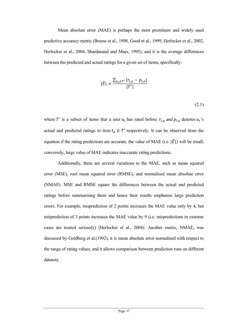
Page 37
Mean absolute error (MAE) is perhaps the most prominent and widely used
predictive accuracy metric (Breese et al., 1998, Good et al., 1999, Herlocker et al., 2002,
Herlocker et al., 2004, Shardanand and Maes, 1995), and it is the average differences
between the predicted and actual ratings for a given set of items, specifically:
| |∑ | , , |
| |
(2.1)
where is a subset of items that a user has rated before. , and , denotes ’s
actual and predicted ratings to item respectively. It can be observed from the
equation if the rating predictions are accurate, the value of MAE (i.e. | |) will be small,
conversely, large value of MAE indicates inaccurate rating predictions.
Additionally, there are several variations to the MAE, such as mean squared
error (MSE), root mean squared error (RMSE), and normalised mean absolute error
(NMAE). MSE and RMSE square the differences between the actual and predicted
ratings before summarising them and hence their results emphasise large prediction
errors. For example, misprediction of 2 points increases the MAE value only by 4, but
misprediction of 3 points increases the MAE value by 9 (i.e. mispredictions in extreme
cases are treated seriously) (Herlocker et al., 2004). Another metric, NMAE, was
discussed by Goldberg et al.(1992), it is mean absolute error normalised with respect to
the range of rating values, and it allows comparison between prediction runs on different
datasets.

Page 38
2.4.1.2 Classification Accuracy Metrics
Classification accuracy metrics measure the frequency with which a
recommender system makes correct or incorrect decision about whether an item is good.
They are also referred to as decision support metrics (Herlocker et al., 2004, Ziegler et al.,
2004). Classification accuracy metrics are commonly used for evaluating recommenders
whose tasks are to recommend a ranked list of the recommended items (i.e. a set of all
good items) (Linden et al., 2003, Shardanand and Maes, 1995, Wei et al., 2005, Ziegler
et al., 2004, Deshpande and Karypis, 2004, Karypis, 2001).
Nowadays, recommenders designed specifically for making item list based
recommendations are very popular, and, therefore, classification accuracy metrics have
been widely applied and many different variations have been developed. Among all
different variations, precision and recall are the most basic classification accuracy
metrics. Precision and recall were initially suggested by Cleverdon in 1966 (Cleverdon
et al., 1966) as evaluation metrics for information retrieval systems. Due to the simplicity
and the popular uses of these two metrics, they have been widely adopted for
recommender system evaluations (Basu et al., 1998, Billsus and Pazzani., 1999, Sarwar
et al., 2000a, Sarwar et al., 2000b, Ziegler et al., 2004). Precision and recall for an item
list recommended to user are computed based on the following equations:
Recall| |
| |
(2.2)

Page 39
Precision| || |
(2.3)
where is the set of all items preferred by user , and is the set of all recommended
items (generated by the recommenders). Based on the Equation (2.2) and (2.3), it can be
observed that the values of precision and recall are sensitive to the size of the
recommended item list (i.e. | |), that is, when the size of the recommended item list is
large, the result precision will be small and recall will be large. In contrast, when the size
of the recommended item list is small, the result precision will be large and recall will be
small.
Since precision and recall are inversely correlated and are dependent on the size
of the recommend item list, they must be considered together to evaluate completely the
performance of a recommender (Herlocker et al., 2004). F1 metric suggested by Sarwar
et al. (2002) is one of the most popular techniques for combining precision and recall
together in recommender system evaluation, and it can be computed by the following
formula:
F12
(2.4)
While precision, recall and F1 metrics are directly adopted from the field of
information retrieval, many of their variants have been suggested for better applicability
in the context of recommender systems. Breese score (also known as weighted recall) is

Page 40
one such notable example. Breese score is proposed by Breese et al. (1998), and it
considers the fact that items at the end of a recommendation list are less likely to be
viewed by the active user. Hence, the quality (i.e. the obtained Breese score) of a
recommendation list also depends how items are arranged in the list. Other popular
classification accuracy metrics include Relative Operating Characteristic (ROC) and
Customer ROC (CROC) metrics (Herlocker et al., 2002, Schein et al., 2002), these two
metrics measure the extent to which an information filtering system is able to distinguish
between signal (user preferred items) and noise (user unseen or disliked items). In
contrast, the NDPM metric employed by FAB recommender system (Balabanović and
Shoham, 1997) considers predictive accuracy for items in the recommendation lists (i.e.
combines both predictive accuracy and classification accuracy metrics), and, therefore,
imposes a higher standard for recommendation list evaluations.
2.4.2 Beyond Accuracy
Although recommendation accuracy is an important facet for recommender
system evaluation, there are still many other factors that can affect users’ satisfaction and
perceptions to a recommender. For example, a recommender might achieve high
accuracy by only recommending popular items; however, some users might find such
recommenders rather boring and expect for recommendations with serendipity. The
following lists some of other facets for recommender evaluation:
Coverage. A recommender with good coverage indicates it is able to make
predictions on most items. Recommenders with lower coverage may be less
valuable to users, because they will be limited in the decisions they are able
to help with (Herlocker et al., 2004). Coverage measure has been the most
popular metric among all non-accuracy based evaluation metrics, and it

Page 41
measures the percentage of elements part of the problem domains (i.e. items
or item categories) for which predictions can be made (Good et al., 1999,
Herlocker et al., 2004, Middleton et al., 2004).
Novelty and Serendipity. Recommenders with novelty and serendipity are
able to make non-obvious recommendations. Some recommenders produce
highly accurate recommendations (i.e. obtain high scores with accuracy
metrics) may still be useless in practice if their recommendations are too
obvious. For example, a recommender in a grocery store might suggest milk
to any shopper who has not yet selected it. Statistically, this recommender is
highly accurate as almost everyone buys milk when they are grocery
shopping. However, such a recommendation is not very useful, because
everyone who comes to grocery store to shop has bought milk in the past,
and knows whether or not they want to purchase more (Herlocker et al.,
2004).
Novelty and serendipity metrics measure the degree to which the
recommenders are presenting items that are both attractive to users and
surprising to them. However, designing these metrics is difficult because
usual methods for measuring accuracy are directly antithetical to novelty
and serendipity. In fact, even though novelty and serendipity have started
getting attentions from researchers (Schafer et al., 2000, Ziegler et al., 2004),
no standard metric for evaluating novelty and serendipity of recommenders
is yet available.
Learning Rate. Given recommenders with similar recommendation
accuracy, it should be obvious that the one requires least amount of data or
information (e.g. rating data) should be superior to others. In general,

Page 42
learning rate metrics measure the amount of information a recommender is
required to produce recommendations with a certain level of accuracy
(Herlocker et al., 2004). Based on different information types, there are three
different learning rate metrics: overall learning rate, per-item learning rate,
and per-user learning rate. The overall learning rate measures the amount of
overall ratings required by a recommender to produce quality
recommendations. The per-item learning rate measures the amount of
ratings to an item are required to allow accurate rating prediction to the item.
The per-user learning rate measures the amount of ratings from an user are
required to allow quality recommendations generated to the user (Herlocker
et al., 2004).
2.5 IMPLICATIONS
In Section 2.1, several classic and state of the art recommender systems are
reviewed. Based on the review, three major information resources employed by
recommender systems for recommendation making are identified, and they are:
item content information (Section 2.1.1)
user demographic data (Section 2.1.3)
users’ past browsing, shopping and rating histories (Section 2.1.2)
Among the three information resources, user rating data is considered the most
popular as it directly relates to users’ personal preferences. However, user rating data is
sometimes difficult to obtain, especially for these new and small ecommerce sites. The
lack of information resources could subsequently affect recommenders’ performances,
and hence result in the cold-start problem (Section 2.1.2 and 2.1.4). Except for
alleviating the cold-start problem in algorithm level (Section 2.1.4), the more

Page 43
fundamental solution is to enrich the information resources. There are two basic ways to
accomplish the enrichment of information resources:
Enrich the information resources by considering other facets of the data.
Enrich the information resources by obtaining more data.
Section 2.2 reviewed a classic example of how other data facets can be utilised to
improve recommendation quality. Researchers have recently suggested that the cold-
start problem can be effectively alleviated by considering item taxonomic information
into recommendation making process (Aroyo et al., 2007, Ziegler et al., 2004). Item
taxonomic information has started getting attentions due to the increasing popularity of
semantic web and ontology related research, and it is considered more sophisticated,
well structured and widely applicable than standard item content information (e.g.
keywords vectors). However, the application of taxonomic information in recommenders
is still relatively new, and most taxonomy-based recommenders simply treat the item
taxonomic information as ordinary content information. Therefore, we believe there is
still a large gap in the effective utilisation of item taxonomic information, and one of the
major goals of this thesis is to explore other promising utilisation of item taxonomic
information to alleviate cold-start problem as well as improve recommendation quality.
One of the most intuitive ways to increase the data volume for a recommender is
to obtain data from other parties, especially from other recommenders. While
recommenders mainly operate over internet, in order to automate the data gathering
progress, it is required to allow multiple recommenders communicate and exchange data
in a decentralised fashion. Hence, studies related to distributed and decentralised
recommender systems were reviewed and investigate (Section 2.3). Based on the review,
most distributed recommender systems are designed for peer-to-peer based applications
and their goal is to move the ownership of recommenders from site owners’ hand to

Page 44
individual user’s hand (i.e. change from B2C to C2C). However, we have not found any
studies on distributed recommenders that address how the cooperation of multiple
recommenders over distributed network can enhance each other’s recommendation
quality as well as alleviate the cold-start problem. As the goal of this thesis is to
investigate novel techniques for alleviating the cold-start problem, it also investigates the
possibility of distributed information sharing for improving their recommendation
quality and resistance to the cold-start problem.
As several novel recommendation techniques are proposed, investigated and
developed in this thesis, it is important to evaluate them and compare them with other
existing techniques. Therefore, in Section 2.4, state of the art evaluation metrics and
various recommender evaluation aspects are reviewed.

Page 45
Chapter 3
3Making Recommendations with Item
Taxonomy
As mentioned in Chapter 1, one of the major issues that recommender systems
are facing is the cold-start problem. This problem often arises in the following situations:
The target user has very few ratings (e.g. a new user). In this scenario,
recommenders (especially collaborative filtering based recommenders)
might not be able to find users with tastes that are truly similar to the target
user, thus, the quality of recommendations to the target user might be poor.
Moreover, it is difficult to obtain the content interests of the target user
because of the very limited number of items rated by the target user.
The amount of explicit rating data in the system is small. Many
recommender systems rely on the explicit ratings to find users with similar
item preferences to the target user. In the case of lacking sufficient rating
data, recommenders may not be able to find similar users and hence to make
quality recommendations.
It can be observed that the major cause for the above two situations is the heavy
dependency and reliance on explicit item rating data for recommendation making.
Indeed, most recommender systems (especially collaborative filtering based ones) make
recommendations based on users’ item preferences, and the item preferences are mainly
extracted from these users’ explicit item rating data. When the amount of explicit rating

Page 46
data is insufficient, the induced item preferences for the users may be, therefore,
inaccurate, and this consequently leads to poor recommendation quality.
A user’s item preference reflects the user’s perceptions to the quality of the items
that he or she has seen or observed. Hence, with the proper use of the item preference
information and collaborative filtering techniques, a user’s potential perception to a
given item’s quality can be predicted. However, a user’s satisfaction to a given
recommended item (or a list of recommended items) may not solely depend on whether
the quality of the item matches the user’s true perception to the item (Herlocker et al.,
2004). There are many other factors that may affect the user’s perception to a given
recommendation, such as the size and the order of the items of the recommended item
list, the novelty or serendipity of the recommendation, the taxonomic relevance of the
recommendation to the user’s taxonomic interests, etc (Herlocker et al., 2004). Hence, in
order to maximise the user’s satisfaction, recommenders should utilise other information
resources rather than solely rely on the explicit rating data.
In this chapter, we explore a new information resource – item (or product)
taxonomic information – to alleviate cold-start problems as well as improve
recommendation quality. Item taxonomy is a set of controlled vocabulary terms or topics,
usually hierarchical, designed to describe and classify items (Levy, 2004). Due to the
drastic growth of information volume, ecommerce sites and Business-to-Business (B2B)
applications, the development and application of item taxonomy are becoming
increasingly popular. For example, the United Nations Standard Products and Services
Classification (UNSPSC) specifies more than 11,000 taxonomy codes and the
hierarchical order to describe and classify products and services for use throughout the
global marketplace (Levy, 2004, Leo et al., 2003). Ecommerce sites such as
Amazon.com (http://www.amazon.com), BARNES&NOBLE (http://www.book.com),

Page 47
art.com (http://www.art.com), eBay (http://www.ebay.com) etc. also provide their own
item/product taxonomy to describe and classify their goods.
This thesis exploits item taxonomic information to obtain users’ taxonomic
preferences from their past ratings and browsing histories. A user’s taxonomic
preferences reflect the user’s interests to the category or catalogue of the items. The main
differences between users’ taxonomic preferences and item preferences is that item
preferences capture users’ perceptual tastes to items, whereas taxonomic preferences
capture users’ content interests to items. Instead of only using users’ item preferences
like what the standard collaborative filtering does, we make use of both users’ item
preferences and taxonomic preferences. In the cases of lacking rating data or for a new
target user, even there might be no similar users according to the target user’s item
preferences, we still can find users who have similar taxonomic preferences with the
target user. Moreover, because we are able to obtain users’ taxonomic preferences from
both their explicit and implicit ratings, we can assure there is sufficient user taxonomic
preferences information for generating quality recommendations even when the amount
of user explicit rating data in the system is small.
This chapter presents two recommendation techniques that make use of item
taxonomic information. The first technique, which is called Hybrid Taxonomy
Recommender (HTR), utilises item taxonomic information to improve the
recommendation quality of standard item-based collaborative filtering systems. The
second technique, which is called Cold-Start Proof Hybrid Taxonomy Recommender
(CSHTR), is developed specifically for systems operating in environments with severe
cold-start problems.

Page 48
3.1 RELATED WORK
Much research has suggested that the cold-start problem can be alleviated by
combining collaborative filtering and content-based techniques (Burke, 2002, Ferman et
al., 2002, Park et al., 2006, Schein et al., 2002). However, as part of the recommendation
process for these hybrid recommenders is content-based, the generated recommendations
may be excessively content centric and lack of novelty (Middleton et al., 2002, Ziegler et
al., 2004). Hence, semantic and ontology based techniques have been suggested to
improve the recommendation generality for the content-based filtering. Middleton
(Middleton et al., 2002) suggested an ontology based recommender which uses external
organisational ontology (e.g. publication-and-authorship relationships, and projects-and-
project membership relationships) to solve the cold-start problem. However, as the
Middleton’s technique is mainly designed for recommending research papers and
documents, and relies on a specific organisational ontology, therefore, it is not easy to
adopt this method for general recommenders. Another work is the taxonomy-driven
product recommender (TPR) proposed by Ziegler et al (Ziegler et al., 2004). TPR utilises
a general, tree structured product taxonomy to enhance its recommendations. Due to the
simplicity of the taxonomy structure, Ziegler’s technique is considered widely applicable
to different domains (Ziegler et al., 2004). To the best of our knowledge, Middleton and
Ziegler’s techniques are the only two studies bearing traits similar to the proposed HTR
and CSHTR techniques. HTR and CSHTR employs similar tree structured taxonomy
used in TPR, and, therefore, they inherit TPR’s generality advantage. However, TPR is
only applicable to use user’s implicit taxonomic preferences for making
recommendations, whereas HTR and CSHTR utilise the relationship between users’
implicit taxonomic preferences and explicit item preferences for recommendation
making, therefore, yielded better recommendation performance and work well in the

Page 49
case of lacking of implicit taxonomic data. Moreover, HTR and CSHTR inherit item-
based collaborative filtering paradigm (Deshpande and Karypis, 2004) (in contrast to
TPR’s user-based collaborative filtering), therefore, most computations can be done
offline which results in significant improvement to the computation efficiency of online
recommendation generation.
3.2 PROPOSED APPROACH
The basic idea behind HTR is intuitive. It firstly finds a set of users (i.e. the
neighbours) with similar item preferences to a given target user, and then extracts
taxonomy topics that are popularly and uniquely preferred by these users. By combining
the taxonomy topics preferred by the target user and his/her neighbours, the taxonomic
preferences of the target user is induced. Finally, HTR estimate the target user’s
preference to a candidate item by combining his/her item preferences with taxonomic
preferences. By utilising both the users’ item preferences and item taxonomic
preferences, HTR offers two major advantages over other existing recommenders based
on only item preferences. Firstly, when two items are both preferred by the target user’s
neighbours, HTR will assign higher score to the item whose taxonomy topics are more
popularly and uniquely preferred by the neighbours. Since extra information resources
(i.e. users’ item taxonomic preferences) are utilised to refine the recommendations,
therefore, better recommendation quality is achieved in HTR. Secondly, for items with
only few or no ratings (e.g. new arrival items), they can still be recommended to users by
HTR if their topics are preferred by the users. As such, HTR effectively alleviated the
cold-start problem caused by dataset with high sparsity in user ratings (i.e. user ratings
cover only a small portion of all items).

Page 50
In the case of severe cold-start problem, HTR might have difficulties in making
quality recommendations, as it might be unable to allocate neighbourhoods for target
users based on their item preferences. CSHTR is specifically designed for such situations.
CSHTR finds target users’ neighbourhoods based on their taxonomic preferences instead
of item preferences, and hence it is capable of obtaining neighbours for target users who
have distinct tastes or few explicit ratings. Based on the neighbourhoods with similar
taxonomic preferences, CSHTR extracts the commonly preferred items from the
neighbours as candidate item lists. It then ranks and suggests these candidate items
according to the target users’ taxonomic preferences.
3.2.1 Notation
Before delving into algorithmic details, in this subsection we formally define the
concepts and entities involved in this research. These definitions will be also used in
subsequent chapters in this thesis and they can be tied easily to arbitrary application
domains.
Users , , … , . All users that have browsed items or
contributed item ratings in the sites are elements of . Possible identifiers
are globally unique names, user ids, URIs, etc.
Items (or Products) , , … , . All domain-relevant items are
stored in set . Possible unique item identifiers can be proprietary product
codes from an ecommerce site (e.g. Amazon.com’s ASINs) or globally
accepted code (e.g. ISBNs, ISSNs, etc.).
Implicit user ratings , , … , . Every user is assigned a set of
items that he or she has implicitly rated. Implicit ratings are
automatically inferred and collected from the user’s non-rating relevant

Page 51
actions (e.g. history of purchases, navigation history and product mentions),
therefore, they usually imply the users’ possible item interests rather than
clear indications of subjective item preferences (i.e. whether the users like or
dislike the items) (Montaner et al., 2003). Hence, usually indicates a set
of items being seen or interested by , and there are no precise values
associated with the items in to indicate the degree of like and dislike to
the items. Similarly, for these items \ that are not implicitly preferred by
, it can only be concluded that these items are unseen or uninterested by
(rather than disliked by ).
In general, implicit ratings are far more obtainable and accessible in
ecommerce sites and online communities than explicit ratings. Therefore,
when they are applied appropriately, implicit ratings can be a good means
for alleviating the cold-start problem (Schwab et al., 2000, Ziegler et al.,
2004).
Explicit user ratings , , … , . Every user is assigned a set of
items that he or she has explicitly rated.
Explicit rating value , contributed by user to item . In
contrast to implicit ratings, explicit ratings are obtained by letting users to
judge items explicitly on a binary scale (e.g. classify an item as ‘like’ or
‘dislike’ or as ‘relevant’ or ‘irrelevant’) or discrete scale (e.g. rank an item
from 1 to 10, 1 indicates ‘dislike most’ and 10 indicates ‘like most’). In
order to express the degree of users’ item preferences in explicit ratings, we
use , to denote user ‘s explicit rating value to item .
Moreover, in order to accommodate different explicit rating scales, we

Page 52
assume the explicit ratings are normalised so that , 0,1 , where 0
indicates minimal satisfaction and 1 indicates maximum satisfaction.
User ratings , , … . All items that user has implicitly or
explicitly rated before, i.e. .
Taxonomic topic set , , … , . Set contains taxonomic topics
or categories for item classification. Each topic represents one
specific subject that items into which may fall. Topics express broad
or narrow concepts, when a topic’s concept is covered by (or is part of)
another, we call the former topic as sub-topic of the latter. We define map
: 2 retrieves all direct sub-topics for topics .
Based on the sub topic relation, we can define a strict partial order on the
topics in set to differentiate between super topics and sub-topics. Formally,
, , if , then is a subtopic of and there is a partial
order between and , denoted as . In addition, for simplicity,
we require that for all , , , so that one
topic can only have one direct super topic. With this requirement and the
map , we can recursively extract the taxonomy tree structure from the set
. Moreover, the same as all standard tree structures, the taxonomy tree has
exactly one top-most element, denoted as , with zero incoming-degree
representing the most general topic. In contrast, for the bottom-most
elements with zero outgoing-degree, they are denoted by and represent the
most specific topics.
An example of item taxonomy is shown in Figure 3.1. Within the item
taxonomy depicted in the figure, ‘ROOT (Books)’ is the root topic (i.e. )
covering the broadest concept, and ‘Apache’ and ‘Unix’ are the leaf topics

Page 53
(i.e. ) expressing the most specific concepts. The map returns the direct
sub-topics for any given topics in the taxonomy, for example,
Web Development Ecommerce,Web Design,Web Servers .
Item taxonomic descriptors , , … , . In order to describe
and classify items, every item is associated with a set of item
taxonomic descriptors . Note, an item can be described with multiple
descriptors because the item might possess a broad range of concepts,
strictly categorising the item under one single concept might be imprecise.
A taxonomic descriptor is a sequence of ordered taxonomic topics, denoted
by , , … , where , , and , , … , . The
topics within a descriptor are sequenced so that the former topics are super
topics of the latter topics, specifically, E and , where
0 . In our system, for any item descriptor , , … , , it is
required that and .
Figure 3.2 shows an example list of items (i.e. books) with their
corresponding item taxonomic descriptors given under ‘Category’. For
example, the first book (‘Book#1’) in this list contains three item taxonomic
descriptors, and their corresponding leave topics (i.e. the most specific topics)
are ‘Apache’, ‘Network Administration’, ‘Network Programming’
respectively. With the defined information model, the item taxonomic
descriptors can be represented by "Book#1" , , , where:
"Books", "Computer & Internet",
"Web Development", "Web Servers", "Apache"
"Books", "Computer & Internet",
“Networking", "Network Administration"

Page 54
Books, Computer & Internet,
“Networking", "Network Programming"
Figure 3.1: An example fragment of item taxonomy extracted from Amazon.com.

Page 55
Figure 3.2: An example list of items with their taxonomic descriptors.
3.2.2 Item Preferences based User Clusters
Clustering has been widely applied in recommender systems (especially
collaborative filtering based ones) to improve the computation efficiency (Cöster et al.,
2002, Sarwar et al., 2002, Jerome and Derek, 2004, Gui-Rong et al., 2005, Rashid et al.,
2006b, Rashid et al., 2006a). As mentioned in Section 2.1.2, collaborative filtering based
recommenders make recommendations to a target user by taking the opinions from other
users with similar item preferences to the target user. The process of finding users with
similar item preferences to the target user is commonly referred to as ‘Neighbourhood
Formation’. While neighbourhood formation is one of the most important steps in
making recommendations, it can also be the major performance bottleneck for
recommenders when the number of users and items in the system is large. The basic idea
behind clustering is to improve the online neighbourhood formation process by utilising

Page 56
offline computed user clusters. Figure 3.3 depicts how neighbourhood searching spaces
can be significantly reduced within the neighbourhood formation process based on the
pre-computed user clusters. Figure 3.3(a) shows that in standard collaborative filtering
recommenders, the target user’s profile (i.e. the circled dot) is compared with all other
user profiles in the dataset (i.e. all other dots within the dashed circle) in order to find the
top closest neighbours. In Figure 3.3(b), users are grouped into small clusters (i.e. dots
within the squares), hence, the searching space for forming the neighbourhood is reduced
within the target user’s cluster.
Figure 3.3: Reduce neighbourhood searching space with clustering
In order to form the neighbourhood for a given target user based on similarity of
users’ item preferences, a similarity measure is required to determine the degree of
similarity between two users’ item preferences. Pearson’s correlation coefficient and
cosine similarity count among the most prominent similarity measures for users’ item
preferences (Breese et al., 1998, Herlocker et al., 2002). In this thesis, Pearson

Page 57
correlation is adopted since it can accommodate the differences between users’ rating
styles (i.e. some users have a preference for the extreme values of the rating scale, while
others rarely deviate from the median) and, therefore, usually leads to better
recommendation quality (Herlocker et al., 2002, Herlocker et al., 2004, Jun et al., 2006).
The Pearson correlation coefficient measure used for computing the item preference
similarity between two users , is defined below:
,∑ , ,
∑ , ∑ ,
(3.1)
where is an item rated explicitly by both and , specifically
and , denote the average explicit ratings made by and . The average explicit
rating for a user can be computed by:
∑ ,
| |
Based on Equation (3.1), the user set can be divided into a set of user clusters
, , … , , such that and . For the sake
of convenience, let denote the cluster that contains user . As the
clusters are constructed based on users’ item preference similarity, users within the same
cluster will have similar item preferences. There are many existing clustering techniques
which can be utilised for producing the user clusters, some widely recognised ones are k-
means, k-modes and x-means (Gui-Rong et al., 2005, Jain et al., 1999, Pelleg and Moore,
2000, Sarwar et al., 2002). Additionally, we have also developed an effective clustering
Page 58
method for recommender systems, HPC, and the detail of this technique can be found in
Appendix B.
3.2.3 Item Preferences - Taxonomic Preference Relation
Most recommender systems make recommendations by exploiting the relations
among users’ item preferences. For example, under the widely accepted assumption that
users must have similar tastes if they have similar item preferences (i.e. similar ratings to
the same items), given a set of items rated by a target user, collaborative filtering based
recommenders make recommendations by exploring other items that have been rated
similarly by the target user’s neighbours (Goldberg et al., 1992, Breese et al., 1998, Mira
and Dong-Sub, 2001, Lemire and Maclachlan, 2005). Recent studies on exploiting users’
taxonomic preferences to make recommendations are also based on an assumption that
users must have the similar content interests if they have similar taxonomic preferences
(Sollenborn and Funk, 2002, Ziegler et al., 2004, Middleton et al., 2002). Intuitively and
based on our observations, in this thesis, we propose the following assumption about the
relation between users’ item preferences:
Assumption 3.1. (Item Preferences - Taxonomic Preference Relation) Users who are
in the same item preference based neighbourhood or cluster share not only similar item
preferences but also similar taxonomic preferences.
In the case of clustering based neighbourhood formation, Assumption 3.1
suggests that the users within one cluster should have apparent similar taxonomic
focuses and the taxonomic focuses of the users in different clusters should be different.
The proposed HTR and CSHTR techniques in this thesis are designed and implemented
based on this assumption. Through our experiments in Section 3.3, we have shown that

Page 59
the proposed techniques have gained significant improvements in recommendation
making in both normal and cold-start environments. Moreover, the validity of
Assumption 3.1 has been verified empirically with the use of information gain measure.
The detailed verification and experiment process is detailed in Section 3.3.2.
3.2.4 Extraction of User’s Taxonomic Preferences
In this section, the techniques we employed to extract users’ taxonomic
preferences are described. In our thesis, users’ taxonomic preferences are considered in
two different aspects, namely ‘personal taxonomic preference’ and ‘cluster taxonomic
preferences’, which are discussed in detail in the following subsections.
3.2.4.1 Personal Taxonomic Preference
A user’s personal taxonomic preference implies the taxonomic topics that the
user has shown his or her interests to in the past. We capture a user’s personal taxonomic
preferences through examining the taxonomic topics from the items that the user has
rated (both implicitly and explicitly) before. In this thesis, because the taxonomic topics
are contained in a taxonomic tree structure and impose a hierarchical relation among
each other (see Section 3.2.1), therefore, the following factors can be considered when
designing a technique to compute users’ personal taxonomic preferences:

Page 60
1) Frequency of a user’s topic interest indication. When two topics
, are in the same level (e.g. if they are both leaf topics), a user
may be more interested in than , if the user has rated more items
belonging to than items belonging to . For example, suppose a user
has browsed the three books in Figure 3.2, he or she might be more
interested in the topic ‘Apache’ than in ‘Java’, because all of these three
books are related to ‘Apache’ and only ‘Book#3’ is related to ‘Java’.
2) Item taxonomic topic hierarchy. When two topics , have the
same frequencies in a user’s item ratings, the user may be more interested
in than , if is a sub-topic of . For example, if a user has only
rated ‘Book#2’ in Figure 3.2, he or she might be more interested in topic
‘Apache’ than ‘Web Servers’ even the frequency of the two topics rated
by the user are the same. It is because there are many other topics under
‘Web Servers’ such as ‘Unix’, ‘Linux’, ‘Windows’, etc., and the topic
‘Apache’ describes a more specific domain concept that is encompassed
by ‘Web Servers’. The user who rated ‘Book#2’ might only be interested
in ‘Apache’ rather than ‘Unix’ and ‘Linux’, hence items belonging to
‘Apache’ would have more chances to be preferred over items only
belonging to ‘Web Servers’.
3) Topic concept coverage. Given two sibling topics , (i.e. is
not ’s super topic, and vice versa), has a broader concept coverage
than if contains more sub-topics than . If and have the
same occurrence frequency in a user’s item ratings, the user might be
more interested in than , as has a narrow coverage and more
likely contains the topics that the user prefers.

Page 61
4) Relevance of concepts in sibling topics. Sibling topics must have
something in common that is captured by their super topics. Given two
sibling topics , , their common features can be observed through
their super topics. If a user has interests in , it is reasonable to think
that the user might also be interested in since and share some
common features.
Ziegler et al. (2004) have proposed a technique to derive user personal
taxonomic preferences from user implicit ratings. We have thoroughly analysed
Ziegler’s technique and found that it has taken all the four factors mentioned above into
consideration. In our work, we adopted Ziegler’s technique to generate user personal
taxonomic preferences. For an user , the user’s personal taxonomic preference
can be modelled by a | |-entry vector, called personal taxonomic profile vector, denoted
as , , , , … , ,| | . Each entry , in represents the degree of ’s
preference or interest (i.e. personal taxonomic preference score) to the topic in (i.e.
). In order to measure the similarity between two profile vectors, user-wise
normalisation is applied, such that:
: ,
| |
where is the normalisation factor that can be any positive number, in this thesis we set
| |.
If item taxonomic data is available, users’ personal taxonomic profile vectors can
be generated from users’ ratings to items because each item is associated with a set of
taxonomic topics. In this thesis, the taxonomic topics related to an item can be obtained
from the item’s descriptors. For the items rated by a user, their descriptors need to
equally contribute scores to the user’s personal taxonomic profile vector. Specifically,

Page 62
for any item rated by user (i.e. ), the score contribution of any ’s
descriptor to ’s profile vector can be computed by:
,| | | |
where | | is the number of items rated by and | | is the number of topic
descriptors of item .
As , is meant to be distributed to topics , , … , in descriptor ,
therefore, it is required that:
,
(3.2)
where is the score assigned to topic , and it can be computed by:
1
(3.3)
where returns the number of topic ’s siblings. In other words,
1 resolves the number of ’s immediate children or sub-topics. is a
propagation factor that permits fine-tuning for the significance of topic specificity and
depth in the profile construction process.
It can be observed in Equation (3.3) , is inversely proportional to the
number of ’s direct sub-topics, and, therefore, may be assigned with a higher
score if it covers a more specific domain concept (i.e. in accordance with the third factor

Page 63
described at the beginning of this section). It can also be observed from the equation that
for any 0 , (when 0 1 ), this allows a
hierarchical score decay from the most specific topic (i.e. ) to the most general topic
(i.e. ). Thus, the second factor (i.e. item taxonomic topic hierarchy) is also satisfied.
Moreover, because the final score , for a topic in a profile vector is
accumulated with multiple that are computed from the descriptors of items rated
by , the first design factor is satisfied. Finally, it can be easily observed that the fourth
factor is also satisfied with this approach, because two descriptors with different leaf
topics might still share common intermediate topics and these common topics might be
assigned with similar topic scores.
A brief example of the taxonomic score computation described above is shown
below:
Example 3.1 Suppose a user has rated the three books listed in Figure 3.2, and
these books are categorised based on the book taxonomy depicted in Figure 3.1. Based
on Equation (3.2) and (3.3), we can calculate how scores are distributed to the topic
entries of ’s personal taxonomic profile vector from any given item’s descriptor. In
this example, we demonstrated how scores are distributed through the first descriptor of
‘Book#1’, that is,
"Books", "Computer & Internet",
"Web Development", "Web Servers", "Apache"
Suppose that 900 defines the normalisation factor for the profile vectors, then the
score assigned to any one of descriptors of ‘Book#1’ amounts to:
,| | | “Book#1” |
9003 3
100

Page 64
Next, as the exact score value for the leaf topic ‘Apache’ is unknown, we let
"Apache" . Based on Equation (3.3), the relative score value for the parent
topic of ‘Apache’ (i.e. ‘Web Servers’) can be computed (assuming the propagation
factor 1):
"Web Servers" "Apache"
"Apache" 11
1 1 2
Similarly, the score for the topic ‘Web Development’ can be computed based upon its
parent topic (i.e. "Web Servers" ):
"Web Development" "Web Servers"
"Web Servers" 11 2
2 1 6
Accordingly,
"Computer & Internet"24
"Books" 96
Next, based on Equation (3.2), the exact topic scores can be computed by solving:
"Apache" "Web Servers" "Web Development"
"Computer & Internet" "Books" ,
Thus,
2 6 24 96100
58.18
Finally, by applying the exact value of to the topics, we can obtain:
"Apache" 58.18
"Web Servers"2
29.09
"Web Development"6
9.70

Page 65
"Computer & Internet"24
2.42
"Books"96
0.61
In Ziegler’s research, the taxonomic profile vectors are compared with each
other to measure the taxonomic preference similarity between two users (therefore, the
user-wise normalisation is required). In contrast, this thesis emphasises the extraction of
these user preferred taxonomic topics using Zeigler’s method, and then merge the
personal topic scores with the cluster taxonomic topic scores (to be discussed in Section
3.2.4.2) to generate a more comprehensive user taxonomic preference profile. In order to
uniformly merge personal topic scores with cluster topic scores, we further normalise the
topic scores obtained from the taxonomic profile vectors with min-max normalisation
technique, and use the normalised topic scores as the personal taxonomic topic scores in
the final personal taxonomic profile vector. Specifically, let , be the topic score to the
topic in a user ’s personal taxonomic profile vector computed using
Ziegler’s method, the user’s final topic preference score to the topic in C can be
obtained by:
_ , , minmax min
(3.4)
where min and max are the minimal and maximal score values in ’s
taxonomic profile vector respectively. After the normalisation, user ’s most
preferred topic will receive the topic score _ , 1 , and the most
disliked topic will receive _ , 0.

Page 66
3.2.4.2 Cluster Taxonomic Preference
As described in Section 3.2.4.1, the personal taxonomic topic preference score
_ , is obtained from converting users’ rating data and can be used to measure
users’ personal topic interests. In order to obtain a more comprehensive profile about a
user’s taxonomic interests, it is necessary to study the taxonomic interests of other users
within the same cluster, group or neighbourhood, since users within the same cluster
usually share similar taxonomic interests as assumed in Assumption 3.1. Therefore, we
propose to estimate the user’s taxonomic preference by combining his or her personal
taxonomic preferences with the cluster taxonomic preferences.
In order to extract the cluster level taxonomic preferences, we firstly build a
cluster-based taxonomy similar to the global taxonomy defined in Section 3.2.1 (i.e. )
for each cluster . Formally, we define the cluster-based topic set:
| , , ,
Further, a corresponding map for topics , such that
extracts the direct sub-topics of . Note, because items that have been rated in one
cluster might not be rated at all in other clusters, therefore, it is possible that the cluster-
based topic set contains only a subset of all topics, specifically . Furthermore,
from , we can also conclude that .
Based on the local cluster taxonomy tree, we can measure the distinctness of a
topic within a local cluster in accordance with the global user set. With the
distinctness, we can determine how popular a topic is in a cluster and how unique a topic
is to a cluster comparing to other clusters. The distinctness can be assessed by the
following equation:

Page 67
_ ,0, _ ,
_ ,_ ,
,
(3.5)
where _ , is the number of user ratings involving taxonomy topic within a
given user set . Specifically,
_ , _ ,
where _ , checks if item belongs to topic ,
_ ,1, | ,
0,
Moreover, in Equation (3.5) is a user defined constant, it is used to filter out
topics that are not popularly interested by users. For example, when is set to 50, a
topic needs to be involved in more than 50 item ratings in order to be considered
important within a given user cluster.
It can be easily observed from Equation (3.5), the higher the computed topic
score _ , , the higher the possibility the taxonomy topic is unique and
popular in cluster . It is because in order to obtain a high value for _ , ,
the value of _ , need to be larger than the given threshold and approach
to _ , . It implies that the topic not only need to be popular for the whole
user set (i.e. ) but also within only one cluster . In contrast, if a topic has high
popularities in multiple clusters (i.e. high _ , values for different clusters),
then it will receive a low value for _ , as _ , will be much
larger than _ , ; it indicates that the topic is not unique in cluster .

Page 68
In order to linearly combine the personal and cluster level taxonomic preference
scores (i.e. _ , and _ , ) together, we also normalise
_ , with min-max normalisation. The normalised cluster level taxonomy
preference score is denoted by _ , , specifically,
_ ,_ , min_sc
max_sc min_sc
(3.6)
where
min_sc min _ ,
max_sc max _ ,
3.2.4.3 Merge Personal and Cluster Taxonomic Preferences
In this thesis, a user’s taxonomic preference is constructed with respect to both
the personal taxonomic interests (as described in Section 3.2.4.1) and the cluster level
taxonomic interests (as described in Section 3.2.4.2). In the aspect of personal taxonomic
interests, the user’s topic interests are investigated. In the aspect of cluster taxonomic
interests, we induce the topics that might be potentially interested by the user through
exploring the taxonomic topic interests of the user’s neighbourhood. Having obtained the
user’s personal taxonomic preference profile and the taxonomic preference profile of the
user’s cluster, we compute the user’s taxonomic preferences by linearly combining the
two profiles. Formally, for user and topic the user’s taxonomic preference
score to is:

Page 69
_ , _ , 1 _ ,
(3.7)
where 0 1 is a user controlled parameter for adjusting the weight between the
personal level and cluster level taxonomic preferences in the final taxonomic preference
score computation.
3.2.5 Hybrid Taxonomy Recommender
In this section, we describe the proposed Hybrid Taxonomy Recommender
(HTR) that incorporates users’ taxonomic preference profiles described in Section 3.2.4
with the item-based collaborative filtering (item-based CF) to improve recommendation
quality.
HTR generates item recommendations by combining the estimates to item
preferences and the estimates to taxonomy preferences. In this section, we firstly explain
the item-based CF technique that has been applied in HTR for item preferences
estimation, then the method to calculate users’ taxonomic preferences, finally the
algorithm to generate a list of recommended items. Item-based CF recommends item
to user based on the item similarity between and the items that have been
rated by . The similarity between two items , is computed based on checking
whether these two items are rated similarly by users (Badrul et al., 2001). Specifically:
_ ,∑ , ,
∑ , ∑ ,
(3.8)

Page 70
where , and , denote user ’s rating to item and respectively. and are
the average ratings of and . is the set of users who have rated both and .
is defined as:
| ,
Note, it is possible that two items are never rated together by a user, i.e. .
In such case, _ , returns a special value that is a label indicating ‘Not
Computable’.
As mentioned above, the preference estimate to item for user is based
on the similarities between and the items \ rated by . In order to achieve
it, we need to find items that are explicitly rated by target user and are computable
with the target item . That is,
, \ | _ ,
Finally, the item preference prediction to item for user can be
computed by:
,
∑ _ , ,,
∑ | _ , |,
(3.9)
As rating values (e.g. , ) are pre-normalised between 0 and 1 as described in
Section 3.2.1, it can be easily observed from Equation (3.9) that the value range of item
preference prediction score (i.e. , ) is also between 0 and 1. When , is close to 1, it
indicates might highly prefer . In contrast, when , is close to 0, it indicates that
might have no interests in .

Page 71
Users’ taxonomic preferences are predicted based on the topic scores computed
by Equation (3.7). Let , denote the prediction of a user ’s taxonomic preference to
item , it can be computed as below:
, _ ,
(3.10)
where | , is the set of item ’s topics.
The recommendation of an item to a user will be determined according to both
the user’s item preference prediction computed using Equation (3.9) and the user’s
taxonomic preference prediction computed using Equation (3.10). In order to
recommend a set of items to a target user , we firstly form a candidate item list
containing all items rated by ’s neighbours (i.e. ) but not yet rated by .
Next, for each item in the candidate list, we compute the item preference score and
taxonomic preference score for the item. The proposed preference score for each
candidate item can then be computed by combining the item preference score ( , ) and
the item taxonomic preference score ( , ) together. Finally, candidate items with
highest preference scores are recommended to the user , and these recommended
items are sorted by their corresponding score values. The complete algorithm is listed
below:

Page 72
Algorithm 3.1 _ ,
Input is a given target user
is the number of items to be recommended
Output a list of items recommended for
1) SET \ , the candidate item list
2) FOR EACH
3) SET , , 1 ,
4) END FOR
5) Return the top k items with highest , scores to .
From line (3) of Algorithm 3.1, it can be observed that the predicted ranking score for an
item is computed by a linear combination of item preference score , and topic
preference score , . The coefficient , computed by Equation (3.11) below is used to
adjust the weight between of , and , :
1 1
(3.11)
where is the ratio between the number of the items that are commonly rated with item
by and other users and the number of the items rated by . Specifically,
| , |
| |
and is a user controlled variable that allows manual adjustment for the weight between
of , and , , such that 0,1 .
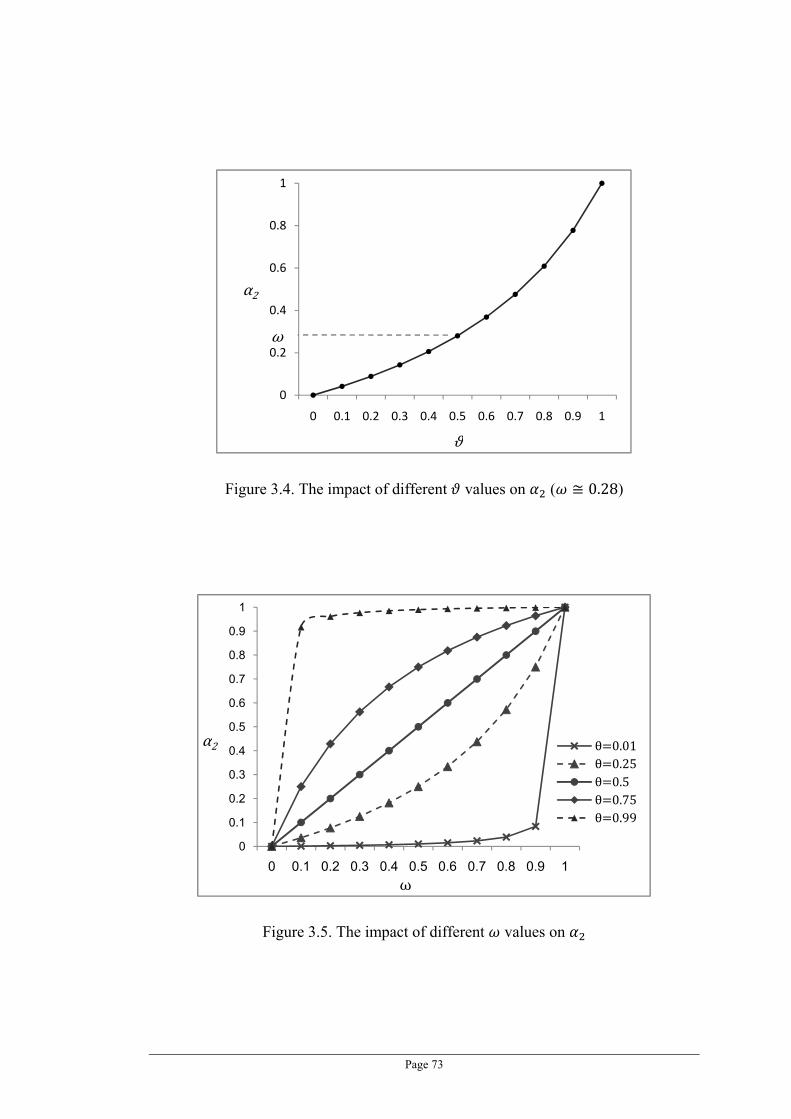
Page 73
Figure 3.4. The impact of different values on ( 0.28)
Figure 3.5. The impact of different values on
0
0.2
0.4
0.6
0.8
1
0 0.1 0.2 0.3 0.4 0.5 0.6 0.7 0.8 0.9 1
α2
ω
0
0.1
0.2
0.3
0.4
0.5
0.6
0.7
0.8
0.9
1
0 0.1 0.2 0.3 0.4 0.5 0.6 0.7 0.8 0.9 1
α2
ω
θ 0.01θ 0.25θ 0.5θ 0.75θ 0.99

Page 74
In Equation (3.11), reflects the confidence to the quality of , , because the
more the target user’s past rated items related to the target item, the higher the accuracy
of the item preference prediction (i.e. , ) will be. When increases will increase
too, thus, , will receive higher weight in the final score (i.e. , ). The relationship
between and with five different settings is depicted in Figure 3.5. It can be
observed from the figure that and are proportional to each other.
Variable , on the other hand, allows manual adjustment of , thus, if is large
(e.g. 0.9) , will still receive high weight even is small. Figure 3.4 and Figure 3.5
demonstrates how can be used to control the value of . When we consider item
preference and item taxonomic preference are equally important in recommendation
making, we can set 0.5. In such a case, as can be easily observed in Equation (3.11),
Figure 3.4 and Figure 3.5, the value of will entirely depend on (i.e. ). The
use of the control variable in the design of the algorithm enables incorporation of
subjective considerations in adjusting the weights of , and , . For example, for
application domains where users’ considerations in item quality outweigh item topic
relevance, can be set to a higher value to allow recommendations mainly depend on
users’ item preferences.
The value (and thus ) is also a good indicator for identifying cold-start
situations. A high value indicates that there exist many users who have commonly
rated the item with the target user, hence there is no cold-start problems. A low or zero
value indicates that there is very few or none users who have commonly rated the item
with the target user, which is one of the cold-start problems.
The value of is automatically adjusted along with the change of the number of
users who commonly rated a given item . The higher the value of , the more the
users who commonly rated the item are (i.e. a normal situation without severe cold-start

Page 75
problems) and, thus, the item preference , estimated based on these users’ rating data
becomes more important and reliable. In this case, the predicted item preference ,
makes a larger contributions to the overall prediction score , than the contribution
made by the predicted taxonomic preference , . On the other hand, if the value of
is low (i.e. a cold-start situation), the taxonomic preference prediction becomes more
important and will contribute more to the overall prediction score , than does the
predicted item preference. This design ensures that taxonomic preferences are used to
supplement or enrich the item preference prediction, especially in cold-start situations.
3.2.6 Cold-Start Proof Hybrid Taxonomy Recommender
By utilising users’ taxonomic preferences, the HTR technique proposed in
Section 3.2.5 is effective even when there is only a small amount of users sharing similar
explicit item ratings to the target user (i.e. when ω is small). However, the proposed
algorithm requires that the given target user can be correctly allocated into one of the
pre-computed user clusters (i.e. ) based on the explicit ratings. Hence,
in severe cold-start situations where the given target user has very distinct tastes and
cannot be allocated to any of the clusters (i.e. ) or his or her explicitly
rated items have not been rated by more than one previous user, the proposed HTR
technique in Section 3.2.5 suffers from the severe information shortage and cannot
make satisfactory recommendations. In this section, we propose another technique,
namely Cold-Start Proof Hybrid Taxonomy Recommender (CSHTR), specifically
designed for making recommendations in the severe cold-start situations. In Section
3.2.3, we suggest that a group of users with similar item preferences might share similar
taxonomic preferences. While the proposed HTR technique applies this rule to discover

Page 76
target users’ potential taxonomy interests for improving recommendation qualities,
CSHTR utilises this rule from the other direction by using the target users’ taxonomic
preferences to discover their potential item preferences. More specifically, instead of
allocating a given target user to a user cluster based on explicit item
preferences, CSHTR finds ’s belonging cluster by comparing ’s taxonomic
preferences with each user cluster’s general taxonomic preferences. For this purpose, we
need to generate users’ taxonomic preferences and each cluster’s general taxonomic
preferences.
The taxonomy vector , , , , … , ,| | as described in Section 3.2.4.1
will be used to represent a user ’s personal taxonomy preferences. The general
taxonomic preferences of a cluster can be obtained by computing the mean
vector of all users’ taxonomy vectors within . Specifically, the taxonomy vector for a
cluster is denoted as:
, , , , … , ,| |
where
,∑ ,
| |
Note, as these taxonomy vectors are mainly used for similarity comparison,
therefore it is not necessary to further normalise these vectors as described in Section
3.2.4.1.
With taxonomy vectors, the taxonomic preference similarities between two
users or between a user and a user cluster can be computed with cosine similarity
measure:

Page 77
_ ,| || |
(3.12)
Based on (3.12) we can find the user cluster that has the most similar taxonomic
preferences with a given user by:
_ argmax _ ,
(3.13)
In severe cold-start situations, based on the taxonomy preference similarity
discussed above, the target user can still be located to a user cluster even
. There are three reasons behind it:
In most cases, the number of taxonomic topics is much smaller than the
number of items (i.e. | | | |). Therefore, the possibility of common
entries in taxonomic topic vectors is much higher than that in item vectors.
Multiple different items might share common topics. For a user who only
rated new items that no one has rated before, it is still possible to find users
with similar taxonomic interests to the user, because there might still be
many items with similar topics to these new items.
Taxonomic topics are organised in a hierarchical tree structure, and impose
hierarchical relations on each other; hence, different topics may be covered
by common super topics. For a user who is interested in a new topic that no
one has known yet, it is still possible to locate the user’s neighbours by
finding users with interests to the super topics of this new topic.

Page 78
However, Equation (3.9) becomes unsuitable for generating item preference for
the target user because the target user may not have any items commonly rated by
previous users, i.e. , . For the severe cold-start situations, we propose
to compute the commonly preferred items within the user cluster and treat these
commonly preferred items as the item preferences of each user in this cluster. A
commonly preferred item can be determined by the popularity of the item in the cluster
and the average of the item’s explicit rating scores given by the users in the cluster who
rated the item. Specifically, the degree of general preference to an item by the
users in a cluster can be computed by:
, , 1 ,
(3.14)
where , is the average explicit ratings to and , measures ’s
popularity in which are computed by:
,∑ ,
| |
(3.15)
,1, | |
| |,
3.16
In Equation (3.15) and (3.16), denotes the set of users in who rated
explicitly, that is:

Page 79
The popularity of an item in a cluster is measured by the number of users in this
cluster who rated the item, the more users who rated the item, the higher the popularity
of the item is. For easy description, we call the number of users who rated an item in a
cluster the Population Value of the item in this cluster. In Equation (3.16), we designed
an upper bound for normalising the popularity score so that , 0,1 . The
upper bound is computed by utilising the common 95% empirical rule (Tabachnick
and Fidell, 2006):
2
where is the average population value of the items in , which is,
∑ | || |
and is the standard deviation of the population values of all items in ,
1| |
In both and , denotes the set of all items being rated by users
in cluster , specifically:
In this thesis, it is assumed that is normally distributed (i.e. under
normal distribution). Therefore, the empirical rule based upper bound allows
approximately 95% items in ’s candidate item list (i.e. ) have a smaller population
value (i.e. ) than . If | | , it means that item is popularly rated and,
therefore, preferred by the users in . In this case we set 1 to , . This design
ensures the value of is set with a reasonable value, so that , can be reasonably
distributed between 0 and 1. That is, when is set too large, most of , values

Page 80
will be very small; when is set too small, most of , values will equals to 1.
Furthermore, one might suggest that setting the upper bound to the maximum value of
| | might be sensible solution, that is:
max | |
However, it is very likely the maximum | | may be in fact an outlier, and
consequently resulting very small , values.
In Equation (3.14), 0,1 is a user controlled variable for adjusting the
weights between the average item preference and item popularity.
Overall, in the severe cold-start situation, a target user’s preference to a given
item is predicted based on the general preference to the item in the user’s belonging
cluster and the taxonomy similarity between the target user and the item. The detailed
CSHTR algorithm is listed below:
Algorithm 3.2 _ _ ,
Input is a given target user
is the number of items to be recommended
Output a list of items recommended for
1) SET _ \ , the candidate item list
2) FOR EACH
3) SET _
4) SET , , 1 _ ,
5) END FOR
6) Return the top items with highest , scores to .
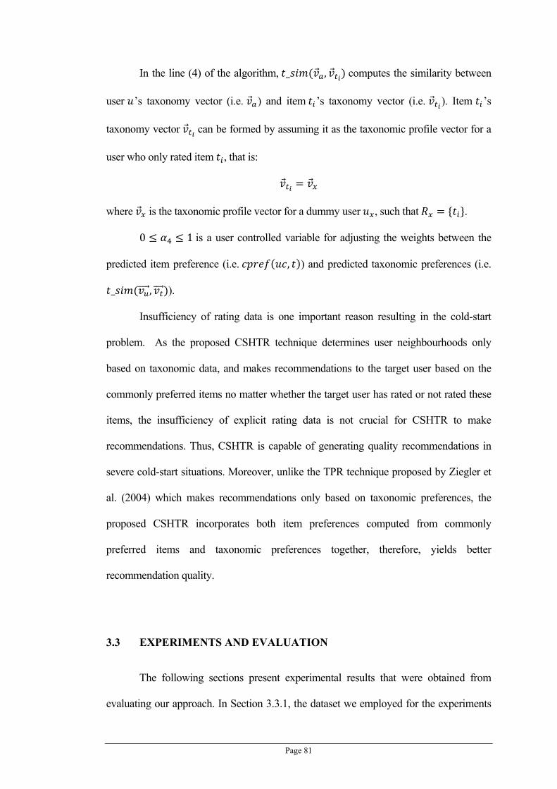
Page 81
In the line (4) of the algorithm, _ , computes the similarity between
user ’s taxonomy vector (i.e. ) and item ’s taxonomy vector (i.e. ). Item ’s
taxonomy vector can be formed by assuming it as the taxonomic profile vector for a
user who only rated item , that is:
where is the taxonomic profile vector for a dummy user , such that .
0 1 is a user controlled variable for adjusting the weights between the
predicted item preference (i.e. , ) and predicted taxonomic preferences (i.e.
_ , ).
Insufficiency of rating data is one important reason resulting in the cold-start
problem. As the proposed CSHTR technique determines user neighbourhoods only
based on taxonomic data, and makes recommendations to the target user based on the
commonly preferred items no matter whether the target user has rated or not rated these
items, the insufficiency of explicit rating data is not crucial for CSHTR to make
recommendations. Thus, CSHTR is capable of generating quality recommendations in
severe cold-start situations. Moreover, unlike the TPR technique proposed by Ziegler et
al. (2004) which makes recommendations only based on taxonomic preferences, the
proposed CSHTR incorporates both item preferences computed from commonly
preferred items and taxonomic preferences together, therefore, yields better
recommendation quality.
3.3 EXPERIMENTS AND EVALUATION
The following sections present experimental results that were obtained from
evaluating our approach. In Section 3.3.1, the dataset we employed for the experiments

Page 82
is discussed. In Section 3.3.2, the suggested assumption about the relationship between
item preference and taxonomic preference (see Section 3.2.3) is verified based on the
information gain technique. Finally, in Section 3.3.3 the proposed HTR and CSHTR
techniques are empirically evaluated.
3.3.1 Data Acquisition
In this thesis, the ‘Book-Crossing’ dataset (http://www.informatik.uni-
freiburg.de/~cziegler/BX/) is chosen to conduct the experiments. The ‘Book-Crossing’
dataset is collected by Cai-Nicolas Ziegler in a 4-week crawl (August / September 2004)
from the Book-Crossing community (http://www.bookcrossing.com/) with kind
permission from Ron Hornbaker, CTO of Humankind Systems. It contains 278,858
users (anonymised but with demographic information) providing 1,149,780 ratings
(explicit / implicit) about 271,379 books. In the user ratings, 433,671 of them are the
explicit user ratings, and the rest of 716,109 ratings are implicit ratings.
The book taxonomy and book descriptors for the experiments are obtained from
Amazon.com. Amazon.com’s book classification taxonomy is tree-structured (i.e.
limited to ‘single inheritance’) and, therefore, is perfectly suitable to the proposed
technique. The average number of descriptors per book is around 3.15, and the
taxonomy tree formed by these descriptors contains 10,746 unique topics.
3.3.2 Verification for Item Preferences - Taxonomic Preference Relation
The assumption we proposed in Section 3.2.3 suggests that the users within one
cluster should have apparent similar taxonomic focus and the taxonomic focuses of the
users in different clusters should be different. In this section, we use information entropy

Page 83
to measure the certainty of user clusters’ taxonomy focuses and empirically validate the
proposed assumption by using information gain measure.
Information gain is commonly used in decision tree construction (Russell and
Norvig, 2002) to measure the increase or decrease in the outcome certainty when
dividing data with a given attribute. When the information gain is high, it indicates that
the divided datasets are more certain about some features. In the case of user clusters
discussed in this chapter, high information gain indicates that the certainty of the
taxonomic focuses of user clusters is high. By adopting the information gain measure,
we can investigate whether different clusters have apparent taxonomic focuses and the
taxonomic focuses are different in different user clusters. The information gain can be
calculated as below:
Pr
(3.17)
where Pr is the probability that an item rating is made by an user in cluster , that
is,
Pr∑ | |
∑ | |
denotes the information entropy for a given user space. The concept of
information entropy is adopted in this thesis to measure the degree of taxonomic focus in
a user set (i.e. a cluster or a neighbourhood). If the information entropy is high for a user
set, then there is no apparent taxonomic focuses in the set (i.e. users in the set prefer all
taxonomy topics equally). In contrast, if the information entropy is low, then it indicates

Page 84
certain topics are popularly preferred within the user set. The information entropy
formula is depicted below:
Pr , Pr ,
(3.18)
where denotes all leaf topics in , that is:
|
and Pr , denotes the probability that the users in the user set are
interested in the taxonomy topic , specifically:
Pr ,∑ | , |
∑ ∑ | , |
where , is the set of items that are rated by and can be categorised by topic ,
specifically:
, | , ,
For a given clustering , , … , , if all are low
, then it means the taxonomic focuses are apparent in all clusters
, according to Equation (3.17), the information gain is high.
Based on the experiment dataset described in Section 3.3.1, we extracted 10,000
users with more than 10 explicit past ratings (i.e. 10) from the 278,858 users in
the entire dataset. k-means clustering technique is then applied to divide these 10,000
users in the dataset into 100 user clusters according to their explicit ratings (detailed
information for user clustering is described in Section 3.2.2). We have tried to produce
different number of clusters for the dataset (i.e. different values for k), and we have
found by setting k to 100 (i.e. 100 clusters) can produce clusters with reasonable qualities.

Page 85
In order to form the baseline of our experiment, we also constructed 100
randomly formed user clusters from the same user set. The population distribution of the
randomly formed user clustering partition is similar to the target clustering partition.
That is,
, | | | |
where is the target clustering partition generated by k-means, and is
the randomly formed partition. For , users within the same cluster have similar
item preferences, in contrast, users within the same cluster of have no apparent
item preference similarities among each other.
Our first experiment is to show if user clusters have stronger taxonomic focuses
than the entire dataset when only explicit ratings are considered. It is shown in the first
column of Table 3.1 the result information gain is 0.823, which is a big increase when
comparing it with the information gain obtained from the randomly formed cluster
partitions (i.e. -0.385). This result shows that, by clustering users with their explicit
ratings, each user cluster has its own taxonomic focuses.
Since our clusters are generated based on only explicit ratings, it might be unfair
if we only consider explicit ratings in calculating taxonomy information gain. Hence, we
further include the implicit ratings in computing taxonomy information gain. With
identical cluster settings, we still get a strong information gain increase (i.e. 0.458) when
comparing to the information gain obtained from the random formed clusters (i.e. -
0.319). Based on the information gain analysis, we can conclude that users within
the same clusters not only share similar item preferences, but they also share
similar taxonomic preferences.

Page 86
Table 3.1. The effect of user clustering on taxonomy information gain
Explicit Ratings Explicit + Implicit
Ratings
users clusters formed based on user ratings ( )
0.823 0.458
Randomly formed user clusters ( )
-0.385 -0.319
3.3.3 System Evaluations
In this section, the computation efficiency and recommendation quality of the
proposed HTR and CSHTR techniques are empirically evaluated.
3.3.3.1 Experiment Framework
In this section, the underling system framework employed for conducting the
experiments is described.
All recommenders being used in the experiment are developed using the Taste
(http://taste.sourceforge.net/) framework that is popularly used for evaluation in
recommender research community. Taste provides a set of standardised components for
developing recommenders, and therefore it ensures the comparability of the developed
recommenders fairly. Moreover, Taste also provides an evaluation framework allowing
researchers or developers to evaluate the performances of their recommenders with a
standardised test bed easily and effectively.
Including the proposed HTR and CSHTR techniques, we have constructed eight
different recommenders in total for the experiments. These recommenders are:

Page 87
Item-based Recommender (IR) Standard item-based collaborative filtering
recommender, the detailed algorithm is given in (Badrul et al., 2001,
Deshpande and Karypis, 2004). This recommender is constructed by
employing the default implementation from the Taste framework, therefore,
the validity of the experiment results is further ensured.
In general, IR computes item preference scores (i.e. , ) for a target user
to all items based on Equation (3.9), and recommends top k
items with the highest item preference scores to . Note, IR only uses
explicit ratings for its recommendation making, and hence implicit rating
data are discarded.
Item-based Recommender with User Clustering (IRC) The item preference
prediction of this recommender is the same as IR, and the only difference
between IRC and IR is that IRC optimises its computation efficiency by
utilising the pre-computed user clusters. More specifically, while IR needs to
compute item preference scores for all items when making a
recommendation for a user , IRC only needs to compute the scores
for items that have been rated in ’s user cluster (i.e.
) .
Slop One Recommender (SO) A well known modern item-based
recommendation technique (Lemire and Maclachlan, 2005), it features on its
implementation simplicity and computation efficiency. The implementation
of this recommender is provided by the Taste framework, so the validity and
accuracy of the implementation is ensured. This recommender utilises only
explicit ratings in its recommendation making process as similar to IR and
IRC. The reason for including SO in the experiments is to ensure that the

Page 88
general recommendation performance achieved with only explicit rating
data can be objectively observed.
The three recommenders mentioned above are existing standard
recommender models. They serve as the benchmark models for this
evaluation.
Taxonomy Product Recommender (TPR) A taxonomy-based
recommender proposed by Ziegler et al. (2004). This study uses similar
taxonomy scheme to our thesis, and therefore can be a good benchmark. For
more details about the TPR, please refer to Section 2.2 and (Ziegler et al.,
2004). Note, TPR uses only implicit rating data for its recommendation
making, and hence explicit rating data are discarded.
Item-based Recommender with TPR (ITR) The combination of the item-
based CF (i.e. IR) and TPR. The hybridisation scheme is identical to HTR
(see Algorithm 3.1). The only difference is that , is computed using
Ziegler’s method (i.e. TPR). As ITR is a hybrid of IR and TPR, therefore, it
utilises both explicit and implicit rating data for its recommendation making
process.
ITR is included in the experiment to allow the proposed HTR technique to
be objectively and fairly evaluated by comparing with the ITR. It is because
both HTR and ITR use explicit and also implicit rating data, while IR, IRC
and SO uses only explicit rating data and TPR uses only implicit ratings
which might make (the comparison between HTR with IR, IRC, SO and
TPR lack of fairness.

Page 89
Hybrid Taxonomy Recommender (HTR) The proposed HTR method as
described in Section 3.2.5, it uses both users’ explicit rating data and implicit
rating data for recommendation making.
Cold-Start Proof Hybrid Taxonomy Recommender (CSHTR) The
proposed CSHTR method as described in Section 3.2.6, it is mainly
designed for severe cold-start situations. CSHTR uses both users’ explicit
rating data and implicit rating data for recommendation making.
Hybrid Taxonomy Recommender (with only explicit ratings) (HTR_E)
The proposed HTR method using only explicit ratings. The purpose of
including this recommender in the experiments is to ensure fair comparison
with IR, IRC, SO, which use only explicit ratings.
3.3.3.2 Parameterisation
In this section, the parameter values we assigned to configure the HTR and
CSHTR techniques for the experiments are detailed.
For the configuration of HTR:
The propagation factor for Equation (3.3) is set to 0.75. This setting
confirms to the configuration suggested by Ziegler et al (2004), and
therefore it ensures the experiment results from our study and (Ziegler et al.,
2004) can be compared. Assigning with values less than 1.0 allows higher
scores to be assigned to the super topics in the taxonomic profile vectors,
and it in turn allows profile vectors with similar scores in their super topic
entries to be considered closer. Amazon.com’s item taxonomy is deeply
nested and topics tend to have many siblings, therefore, topics in higher
levels (i.e. super topics) tend to have very small score values. By setting

Page 90
with a smaller value (i.e. 0.75), we ensure the score distributions for the
profile vectors constructed from Amazon.com’s item taxonomy are more
sensible.
The filter parameter for Equation (3.5) is set to 50. Therefore, a topic
needs to be involved in more than 50 item ratings in order to be considered
important within a given user cluster (i.e. receive _ , score
with value larger than 0).
The adjustment parameter for Equation (3.7) is set to 0.4. This setting put
slightly higher emphasis on the personal level taxonomic preferences for the
final item taxonomic preference score computation (i.e. _ , )
(therefore, less emphasis on the cluster level taxonomic preferences).
The adjustment parameter for Equation (3.11) is set to 0.6. This setting put
slightly higher emphasis on item preferences than item taxonomic
preference for the final recommendation ranking score computation (i.e.
, in Algorithm 3.1).
For the configuration of CSHTR:
The adjustment parameter for Equation (3.14) is set to 0.7. Therefore, in
the computation of cluster ‘s general preference to item (i.e.
cpref uc, t ), there are more emphasis on ’s average item preference to
item than ’s popularity in .
The adjustment parameter for the final recommendation ranking score
computation (i.e. , in Algorithm 3.2) is set to 0.5. This setting put the
same emphasises on both predicted item preference (i.e. , ) and
taxonomic preferences (i.e. _ , ).

Page 91
3.3.3.3 Evaluation Metrics
For the recommendation quality evaluation, we randomly divided each user
‘s past ratings (i.e. ) into two parts, one for training and another for testing. We
use to denote ‘s training rating data and to denote the testing rating data, such
that , , and | | | |. The testing data actually consists of
three types of items, and they are:
Items implicitly rated by :
Items preferred by : | , , , is the average
rating of user ’s explicit ratings.
Items not preferred by : \
In the experiment, the recommenders recommend a list of items to based
on the training set , and the recommendation list will then be evaluated with or .
There are two objectives in this experiment. The first objective is to evaluate
whether a recommender’s performance can be improved by incorporating the item
taxonomy information and the suggested assumption for the relation between item
preference and item taxonomic preference into the recommendation making process (i.e.
whether the proposed HTR technique outperforms other techniques). The second
objective is to evaluate whether the proposed CSHTR can cope with severe cold-start
situations. For the first objective, as the goal is to evaluate the recommenders’ ability to
recommend user preferred items, therefore, only is used to evaluate the resulting
recommendation list . For the second objective, because in the cold-start situations
recommender systems usually don’t possess sufficient rating data and | | might be very
small, therefore, the evaluation standard for recommenders in severe cold-start situations
is relaxed so that will be used to evaluate .

Page 92
In order to evaluate the performances of different recommenders based on and
, recommendation list based evaluation metrics (i.e. classification accuracy metrics)
such as precision and recall, Breese Score, Half-life, and etc. (Herlocker et al., 2004,
Schein et al., 2002) can be utilised, for more details about these metrics please refer to
Section 2.4.1.2. In this thesis, the precision and recall metrics are used for the evaluation,
and their formulas are listed below:
| |
| |
(3.19)
| || |
(3.20)
Note, for the evaluation of CSHTR (for cold-start problems), is replaced with
for both precision and recall measures.
In order to provide a general overview of the overall performances, 1 metric is
used to combine the results of Precision and Recall, details about the 1 metric is
provided in Section 2.4.1.2.:
12
(3.21)
For the computation efficiency evaluation, the average time required by
recommenders to make a recommendation will be compared.

Page 93
3.3.3.4 Experimental Results
Corresponding to the two evaluation objectives addressed in Section 3.3.3.3, two
different testing datasets are constructed for different evaluation objectives. Each record
in the datasets consists of the testing ratings of one user . The first testing dataset
(denoted as NOR_testing) is constructed by randomly choosing 10,000 users from the
278,858 users in the entire Book-Crossing dataset mentioned in Section 3.3.1. The first
dataset is used to evaluate recommenders in normal situations (i.e. without specific cold-
start problems), where the neighbourhoods of these users in the dataset NOR_testing can
be formed (or found) with high item preference similarity. The second testing dataset
(denoted as CS_testing) is used to evaluate recommenders in severe cold-start situations.
This set is constructed by choosing 2,000 users with item preferences dissimilar to all
user clusters (i.e. unable find to form neighbourhoods with similar item preferences, i.e.
c ). The details of the two testing datasets are given in Table 3.2.
Table 3.2. Information for the two different testing datasets
NOR_testing CS_testing
Number of users 10000 2000
Average number of explicit ratings
9.77 3.24
Average number of implicit ratings
18.45 8.47
Experiment Results for dataset NOR-testing
We start by evaluating the recommenders’ recommendation qualities for the
normal user set. We let each recommenders recommend a list of items to each of these
10,000 users, and different values for ranging from 5 to 25 are tested. For this part of

Page 94
the experiment, CSHTR is excluded as it is designed specifically to be operated in cold-
start situations.
The results of this part of the experiment are shown in Figure 3.6, Figure 3.7 and
Figure 3.8. It can be observed from the figures that, for all the three evaluation metrics,
the proposed HTR technique achieves the best result among all the recommenders. In the
case of using only explicit rating data, the recommendation quality of HTR (i.e. HTR_E)
still outperforms other recommenders even slightly degrading compared with using both
explicit and implicit rating data (i.e. HTR performs the best and HTR_E performs the
second best).
The standard item-based CF recommender (IR) performed very similarly to the
Slope One recommender (SO), however, it seems that slope one recommender is slightly
better in recommending longer item lists.
In the experiment, the clustering-based CF recommender (IRC) performed better
than the standard one (IR). The only difference between these two recommenders is in
the candidate item list formation process. The standard item-based CF uses all items
from the dataset as its candidate item list (i.e. \ ) , whereas the clustering-based
version uses only items within a user cluster (i.e. \ ). Intuitively,
the clustering-based CF might perform worse than the standard one, because its
candidate item list is formed from a cluster that is only a subset of the entire item set,
some potential promising items might be excluded and, thus, will not be recommended.
However, based on our observation, many of these excluded items are noises generated
from the item similarity measure (some item similarity measures might generate
prediction noise, please refer to (Deshpande and Karypis, 2004) for more information),
therefore, removing these items from the candidate list can actually improve the
recommendation quality. The proposed HTR also gets benefits from the clustering

Page 95
strategy as it generates recommendations from the candidate item list formed from a
cluster.
Figure 3.6. Recommender evaluation with precision metric
0
0.02
0.04
0.06
0.08
0.1
0.12
0.14
0.16
0.18
0.2
#5 #10 #15 #20 #25
Precision
top k recommened items
IRC IR SO HTR
TPR HTR_E ITR

Page 96
Figure 3.7. Recommender evaluation with recall metric
Figure 3.8. Recommender evaluation with F1 metric
0
0.02
0.04
0.06
0.08
0.1
0.12
#5 #10 #15 #20 #25
Recall
top k recommened items
IRC IR SO HTR
TPR HTR_E ITR
0
0.02
0.04
0.06
0.08
0.1
0.12
#5 #10 #15 #20 #25
F1
top k recommened items
IRC IR SO HTR
TPR HTR_E ITR
Page 97
Figure 3.9. Computation efficiency results for different recommenders (average
seconds per recommendation)
From the results shown in the Figure 3.6, Figure 3.7 and Figure 3.8, we can see
that the TPR technique described in (Ziegler et al., 2004) performed the worst among all
recommenders in our experiments. This is because TPR uses only implicit ratings as its
data source and generates recommendations only based on taxonomy preferences,
whereas in our evaluation scheme (see Section 3.3.3.3) recommendations are evaluated
based on these explicitly preferred items (i.e. ). In order to make the proposed HTR
and Ziegler’s TPR more comparable, we modified TPR by adding the item-based CF
component into TPR resulting in the new recommender ITR. ITR performed better than
the standard TPR as it included the item preference in its recommendation making
process. However, it is still worse than all other recommenders (i.e., TPR performs the
worst and ITR performs the second worst). The difference between HTR and ITR is that
the method to compute the taxonomy preferences is different (they use the same method
to compute the item preferences). The result of HTR outperforming ITR indicates that
0.0017
5.6664
5.0825
0.0861
1.5441
0.0473
2.0355
0
1
2
3
4
5
6
IRC IR SO HTR TPR HTR_E ITR
seconds
recommender types

Page 98
users’ item preference is also helpful for generating users’ taxonomy preference. The
proposed HTR technique considers the item preference implication when generating the
taxonomic preferences (i.e. the taxonomic preferences are extracted from user clusters
that are divided based on users’ item preferences). In contrast, TPR generates users’
taxonomic preferences purely from taxonomy data without using any of the users’ item
preferences.
In the experiment, the recommender with the best computation efficiency is the
clustering based CF (IRC) as shown in Figure 3.9. Computation efficiency results for
different recommenders (average seconds per recommendation), and it is much faster
than the standard CF because its candidate item list is much smaller. The proposed HTR
methods (HTR and HTR_E) perform the second and the third best, as they spent a bit
more time on predicting taxonomic preferences comparing to IRC. However, this extra
computation complexity is trivial, because most of these computations (i.e. computing
_ for each user cluster) can be done offline. HTR_E performed slightly better
than HTR because it uses less data (only explicit ratings) to make recommendations.
Ziegler’s TPR is computation expensive because it needs to convert all users and items
into high dimensional taxonomy vectors. ITR performed slightly worse than TPR
because it needs to compute extra item preference predictions using standard CF
technique. Standard item-based CF (IR) technique is the most inefficient one among all
the recommenders, as it needs to build entire candidate item list from scratch and
compute correlations between the user profile and the candidate items for making each
recommendation. In contrast, Slop One recommender (SO) offers a slight advantage in
computation efficiency by pre-computing the correlations between the user profiles and
the items in advance, however, as forming the candidate item lists is still a lengthy

Page 99
process, it is still not as efficient as other techniques with pre-computed candidate item
lists (extracted from the pre-computed user clusters).
Parameterisation Analysis for HTR
In Section 3.3.2, the suggested assumption for the relation between item
preference and item taxonomic preference is verified, and the relation is applied and
utilised by the proposed HTR and CSHTR techniques. In the last section, our experiment
demonstrated that the proposed HTR technique is superior to other existing
recommenders in both recommendation quality and computation efficiency. However,
what has not been shown in the experiment is whether HTR’s superior recommendation
quality in the experiment is indeed resulted from the integration of item preference and
item taxonomic preference.
In order to demonstrate the integration of item preference and item taxonomic
preference does affect the recommendation quality of HTR, we evaluate HTR’s
performance with different settings to the adjustment parameter (in Equation (3.11)).
As described in Section 3.2.5, the adjustment parameter controls the weight
distribution between item preference and item taxonomic preference in the final ranking
score computation. When the value of equals to 1, HTR considers only item
preference (i.e. , ) in its recommendation making process, and therefore behaves
similar to the standard Item-based CF (i.e. IR or IRC). Conversely, when the value of
approaches to 0, only item taxonomic preference (i.e. , ) is considered in the final
ranking computation.
Besides , the adjustment parameter in Equation (3.7) is also investigated in
this section for its relation to the recommendation quality of HTR. It is mentioned in
Section 3.2.4.3 that is used to adjust the weights of personal level taxonomic

Page 100
preference (i.e. _ , ) and cluster level taxonomic preference (i.e.
_ , ) in the final taxonomic preference score computation (i.e. , ),
therefore by experimenting different values in the performance evaluation we can
investigate whether the integration of personal and cluster level taxonomic preference is
beneficial to HTR.
Figure 3.10. F1 results for HTR with different and configurations.
In the experiment, different value combinations of and have been used to
configure HTR, and the performance results (captured and measured based on the F1
metric) obtained from different HTR configurations are depicted in Figure 3.10.
In order to ensure the fairness of the investigation, for different value
combinations of and , all other parameter configurations are kept the same (see
Section 3.3.3.2 for the detail of HTR’s parameter configurations). In this experiment, we
let HTR to recommend top 10 items (i.e. 10) as this setting has resulted in the best
00.2
0.40.6
0.81
0.03
0.04
0.05
0.06
0.07
0.08
0.09
0.1
00.2
0.40.6
0.81
α1
F1
0.03‐0.04 0.04‐0.05 0.05‐0.060.06‐0.07 0.07‐0.08 0.08‐0.09

Page 101
recommendation quality in previous experiments (i.e. in comparison to
5, 15, 20 or 25).
Figure 3.11. F1 results for HTR with different configurations ( 0.2)
Figure 3.12. F1 results for HTR with different configurations ( 0.8)
0
0.01
0.02
0.03
0.04
0.05
0.06
0.07
0.08
0.09
0.1
0 0.1 0.2 0.3 0.4 0.5 0.6 0.7 0.8 0.9 1
F1
0.08
0.082
0.084
0.086
0.088
0.09
0.092
0.094
0.096
0.098
0.1
0 0.1 0.2 0.3 0.4 0.5 0.6 0.7 0.8 0.9 1
F1
α1

Page 102
In order to provide better observations for ’s effect on the performance of HTR,
a 2D graph showing HTR’s performance with different configurations of ( 0.2
remains static) is extracted from Figure 3.10 and depicted in Figure 3.11. It can be
observed from Figure 3.10 and Figure 3.11 that, HTR yielded very low recommendation
quality when approaches to 0 or 1, and it performed well when is between 0.2 and
0.8 (despite the value of ). Hence, the result suggests that the integration of item
preference and item taxonomic preference information is indeed significantly beneficial
for making quality recommendations.
Similar to Figure 3.11, Figure 3.12 depicts a 2D graph showing HTR’s
performance with different configurations of ( 0.8 remains static). It can be
observed from Figure 3.10 and Figure 3.12, HTR achieved best performance in
recommendation quality when both personal level taxonomic preference (i.e.
_ , ) and cluster level taxonomic preference (i.e. _ , )
are considered (i.e. 0.2). By comparing Figure 3.11 and Figure 3.12, it can be seen
that has less effects to HTR’s performance than , that is, the range of performance
difference for is about 0.0045 (from 0.0905 to 0.0959) and for is about 0.06 (from
0.035 to 0.0959). Even though integrating both cluster and personal level taxonomic
preference resulted better recommendation quality, however, the amount of
improvement achieved is small (i.e. 0.0045). Therefore, if further computation efficiency
optimisation is required, little recommendation quality advantage can be sacrificed by
skipping the computation of personal level taxonomic preference (i.e. set 1). The
computation of cluster level taxonomic preference is more efficient than personal level
taxonomic preference as it can be pre-computed offline and shared by multiple users,

Page 103
hence, if only cluster level taxonomic preferences are required, the efficiency of the
proposed HTR technique can be effectively improved.
Based on the experiment results shown in Figure 3.10, Figure 3.11 and Figure
3.12, it can be concluded that a recommender’s recommendation quality can be
improved and benefited by:
Integrating users’ item taxonomic preferences and item preferences together
into recommendation making.
Integrating cluster level and personal level taxonomic preferences together
for extracting users’ item taxonomic preferences.
Experiment Result for dataset CS-testing
In this part of experiment, we evaluate the performance of the proposed CSHTR
under cold-start conditions (i.e. with the user set CS-testing). The baseline recommender
for this evaluation is Ziegler’s TPR, because TPR is the only technique among the others
that is specifically designed for making recommendations in severe cold-start situations.
Except for the CSHTR and TPR, all the other six recommenders listed in Section 3.3.3.1
are not included in this evaluation as they are generally sensitive to cold-start problems
and do not perform well in the cold-start situation (it is because they make
recommendations mainly based on explicit item rating data).
The evaluation results for the cold-start situation are shown in Figure 3.13,
Figure 3.14 and Figure 3.15. The comparison of computation efficiency between
CSHTR and TPR is shown in Figure 3.16. It can be seen from the results that, the
recommendation quality of the proposed CSHTR is better than that of Ziegler’s TPR. It
suggests that the use of common item preferences in the target users’ belonging cluster is
beneficial for alleviating cold-start problems. Moreover, CSHTR offers much better

Page 104
computation efficiency than does TPR, mainly because CSHTR uses the expensive
taxonomy vector similarity computation only for computing the similarity between the
target user and the candidate items, whereas TPR computes the similarities for all users
within their neighbourhood as well as the candidate items.
Figure 3.13. Recommender evaluation under cold-start situations with precision
metrics
Figure 3.14. Recommender evaluation under cold-start situations with recall metrics
0
0.001
0.002
0.003
0.004
0.005
0.006
0.007
0.008
0.009
#5 #10 #15 #20 #25
Precision
top k recommened items
CSHTR
TPR
0
0.001
0.002
0.003
0.004
0.005
0.006
0.007
0.008
0.009
#5 #10 #15 #20 #25
Recall
top k recommened items
CSHTR
TPR

Page 105
Figure 3.15. Recommender evaluation under cold-start situations with F1 metrics
Figure 3.16. Computation efficiencies for CSHTR and TPR
3.4 CHAPTER SUMMARY
In this chapter, we investigated the implicit relations between users’ item
preferences and taxonomic preferences, suggested and verified that users that share
0
0.001
0.002
0.003
0.004
0.005
0.006
0.007
#5 #10 #15 #20 #25
F1
top k recommened items
CSHTR TPR
0.0426
0.4779
0
0.1
0.2
0.3
0.4
0.5
0.6
CSHTR TPR
seconds
recommender types

Page 106
similar item preferences may also share similar taxonomic preferences. Based on this
investigation, we proposed a novel, hybrid technique HTR to automated
recommendation making based upon large-scale item taxonomies that are readily
available for diverse ecommerce domains today. An HTR’s extension, CSHTR, is also
proposed specifically for alleviating the cold-start problems.
HTR and CSHTR produce quality recommendations by incorporating both users’
taxonomic preferences and item preferences. Moreover, these two proposed techniques
can utilise both explicit and implicit ratings for recommendation making, and hence they
are less prone to suffer from the cold-start problems. We have compared the proposed
HTR technique with some standard benchmark techniques, such as item-based
recommender and some advanced modern techniques such as TPR. We have conducted
extensive experiments that demonstrated that the proposed HTR outperforms other
recommenders in both recommendation quality and computation efficiency. In addition,
our evaluation has shown that the proposed CSHTR method performs effectively under
the cold-start situations, and it outperformed the baseline technique, TPR, in both
recommendation quality and computation efficiency.

Page 107
Chapter 4
4Distributed Recommendation Making
In Chapter 3, the possibility of alleviating the cold-start problem by enriching
information resources with additional data facets is examined and demonstrated.
Specifically, the widely available data source, item taxonomy, is investigated and studied
for its applicability in recommender systems. We identified an implicit relation between
users’ item preferences and item taxonomic preferences, and successfully utilised this
relation to alleviate the cold-start problem as well as improve recommendation quality.
In this chapter, another strategy for alleviating the cold-start problem is explored,
that is, to increase data volume of recommenders via allowing them to share and
exchange data and resources with each other over a distributed environment. As
mentioned previously, most of the existing recommender systems are implemented for
one organisation (i.e. business to customer (B2C) recommenders), and in general one
single organisation may not possess sufficient information or data for analysis in order to
give their customers precise and high-quality recommendations (hence results in the
cold-start problem). Therefore, it can be beneficial if organisations can share their
resources (i.e. products and customer database) and recommendations boundlessly (i.e.
build recommendation systems at inter-organisational level), and more importantly, great
business value might be generated by the resource sharing among the organisations.
In this chapter, we present a framework for distributed information sharing
among recommenders. The proposed distributed framework is different from existing
distributed recommender systems. The existing distributed recommender systems are
mainly designed for C2C (Customer to Customer) based applications (such as P2P and

Page 108
file sharing applications), the proposed distributed recommender system introduces
additional B2B (Business to Business) features on top of the standard B2C (Business to
Customer) recommender systems.
This chapter roughly consists of two parts. In the first part, we explain the
rationale of the proposed distributed recommender system, and then describe and discuss
the system models and infrastructures. In the second part, we describe and discuss in
details a recommender peer profiling and selection strategy designed for the proposed
distributed recommender system.
4.1 RELATED WORK
Section 2.3 has comprehensively reviewed existing distributed recommender
systems. This section mainly discusses and compares works that bear strong
resemblance to the proposed distributed recommender framework.
Wei (2003) has proposed an multi-agent based recommender system in which
the recommender system is considered as a marketplace consisting of one auctioneer
agent and multiple bidder agents. Each bidder agent is considered as a recommendation
algorithm that is capable of generating recommendations independently, and within the
marketplace these bidder agents compete to each other for short-listing their
recommendations. The task of auctioneer agent is to incorporate the bids of the bidder
agents and generating the most suitable result to the users. Essentially, Wei’s approach is
a hybridised recommender system designed based on the concept of multi-agent system.
Even though Wei’s system is designed to work within a single organisation and is not
considered as a distributed recommender system, it is still mentioned here as it takes the
concept of decentralised decision making into consideration (i.e. making
recommendations based on the cooperation of multiple recommender agents).

Page 109
As mentioned previously, most existing studies on distributed recommender
systems are mainly designed for peer-to-peer (P2P) or file sharing applications (which
usually adhere to C2C paradigm). We have discussed many relevant studies in this
category in Section 2.3, here we would like to address Awerbuch’s (2005) work in
particular, as it provides a generalised view to these distributed recommenders.
Awerbuch suggested a formalised model for the C2C distributed recommender systems.
In Awerbuch’s model, for the distribute system with users and items, there will be
recommender systems (i.e. agents or peers), and each of the recommender agents will
associate with exactly one user. Each recommender works on behalf of the associated
user either to trade recommendations with other agents or probe the items on its own.
Each recommender aims to finally discover the items preferred by the associated user,
where . In Awerbuch’s opinion, from the perspective of the entire distributed
recommender system, the goal is rather similar to the ‘matrix reconstruction’ proposed
by Drineas et al. (2002); the overall task is to reconstruct an user preference
matrix in a distributed fashion. It can be observed that many distributed recommender
systems can fit into such model.
Generally, the goal of these C2C based distributed recommenders is to avoid
central server failure and protect user privacy (no central database containing
information about customers) (Awerbuch et al., 2005, Castagnos and Boyer, 2007, Han
et al., 2004, Liu et al., 2007, Sorge, 2007, Tveit, 2007, Vidal, 2004, Wang et al., 2006,
Ziegler and Golbeck, 2007) . However, most of them are not aimed at improving their
effectiveness or the recommendation quality. In contrast, the goal of the distributed
recommender system we proposed is aiming at improving the recommendation quality
and alleviating the cold-start problem. Hence, the infrastructure of the proposed
distributed recommender system is different from Awerbuch’s model as well as many

Page 110
other existing systems. Our system contains a set of classical recommenders, and each of
them serves their own set of users. Our goal is to improve the recommendation quality of
these recommenders by allowing them making recommendations for others in a
decentralised fashion. Thus, for the profiling and selection problem, we proposed a more
sophisticated strategy rather than random sampling for recommender peers to explore
others.
Moreover, recommender systems and information retrieval (IR) systems are
generally considered similar research fields (Herlocker et al., 2004, Sarwar et al., 2002),
since both of them try to satisfy users’ information needs by either retrieving the most
relevant documents or recommending the most preferred items to users. Information
retrieval retrieves documents based on users’ explicit queries, while recommender
systems recommend items or products based on users’ previous behaviour. In distributed
IR (Christoph, 1997, Kretser et al., 1998), the entire document collection is partitioned
into sub-collections that are allocated to various provider sites, and the retrieval task then
involves:
Querying minimal number of sub-collections (to improve the efficiency),
and ensure the selected sub-collections are significant to uphold the retrieval
effectiveness.
Merging the queried results (fusion problem) that incorporate the differences
among the sub-collections in such a way that no decrease in retrieval
effectiveness is effectuated with respected to a comparable non-distributed
setting.
For distributed recommender systems, the recommender peer selection and
recommendation result merging are also two important tasks. In fact, one of the major
research focuses of our research is to design an effective recommender peer profiling and

Page 111
selection strategy. The selection criteria for distributed IR including the efficiency
(selecting minimal number of sub-collections) and effectiveness (retrieving the most
relevant documents) is similar to the criteria for the proposed distributed recommender
system. However, in distributed IR, the collection selection is content-based (Christoph,
1997, French et al., 1999, Kretser et al., 1998) and it requires the sub-collections provide
or use sampling techniques to get sub-collection index information (e.g. the most
common terms or vocabularies in the collection) and statistical information (e.g.
document frequencies). In contrast, the proposed selection technique requires no content
related information about recommender peers (assuming recommender peers share
minimal knowledge to each other), the proposed selection algorithm is based on the
observed previous performance (i.e. how well a recommender peer’s recommendations
satisfy the users) about each of the recommender peers.
4.2 ECOMMERCE-ORIENTED DISTRIBUTED RECOMMENDER
As mentioned earlier, the goal of the proposed distributed recommender system
is to allow standard recommenders to overcome cold-start problem and improve
recommendation quality by cooperating, interacting and communicating with
recommenders of other parties (e.g. other ecommerce sites). Hence, the proposed system
is designed to contain of a set of recommenders from different sites and each of these
recommenders is associated with their own users. It is important to note that is possible
that a user might visit multiple sites, and therefore two or more recommenders may share
common users. Similar to the centralised paradigm, each recommender peer in the
proposed system still serve its own users in a centralised fashion (i.e. the recommender
stores all its user and product data in a central place within the recommender). However,
in the proposed system, the recommender peers can enrich their information resources

Page 112
by communicating and cooperating with each other. A general overview of the proposed
system is depicted in Figure 4.3.
Since the proposed distributed recommender system is designed to benefit
ecommerce sites (rather than focusing on helping users to gain more controls on
recommenders), we therefore named our system as ‘Ecommerce-oriented Distributed
Recommender System’, and abbreviated it to EDRS. We also abbreviate the standard
Distributed Recommender System to DRS and Centralised Recommender System to
CRS in order to clarify and differentiate the three different system paradigms.
Before explaining the proposed distributed recommender framework in more
detail, some general differences among the EDRS, DRS and CRS are investigated. In
particular, these systems are compared according to the following aspects:
Ecommerce Model: Based on the general ecommerce activities and
transactions involved in the recommenders’ host application domains, we
can roughly categorise them into three different models, namely, Business-
to-Business (B2B), Business to Customer (B2C) and Customer to Customer
(C2C). In B2B model, activities (e.g. transactions, communications and
interactions) mainly occur among businesses. In the B2C model, activities
are mainly between businesses and customers, and the most typical example
is activities of E-businesses serving end customers with products and/or
services. Finally, the C2C model involves the electronically facilitated
transactions between consumers. A typical example is the online auction
(e.g. eBay), in which a consumer posts an item for sale and other consumers
bid to purchase it.
Architectural Style: An architectural style describes a system’s layout,
structure, and the communication of the major comprising system modules

Page 113
(or software components). Over past decades, many architectural styles have
been proposed, such as, Client-Server, Peer-to-Peer (P2P), Pipe and Filter,
Plugin, Service-oriented, etc. Client-Server and Peer-to-Peer are the two
major architectural styles related to our thesis, and therefore will be
explained in more details. The Client-Server architecture usually consists of
a set of client systems and one central server system, client systems make
service requests over a computer network (e.g. internet) to the server system,
and the server system fulfils these requests. Peer-to-Peer architecture
consists of a set of peer systems interacting with each other over a computer
network, and it does not have the notion of clients and servers, instead, all
peer systems operate simultaneously as both servers and clients to each other.
Communication Paradigm: Based on how two types of entities
communicate with each other within a system, three major communication
paradigms have been proposed, and they are One-to-One, One-to-Many and
Many-to-Many communication paradigms (or relationships). In One-to-One
communication paradigm, communication occurs only between two
individual entities, example applications include: e-mail, FTP, Telnet, etc. In
contrast, a website that displays information accessible by many users is
considered having a One-to-Many relationship. In Many-to-Many paradigm,
entities communicate freely with many others, example applications include:
file sharing (multiple users to multiple users), Wiki (multiple authors to
multiple readers), Blogs, Tagging, etc.
Figure 4.1 shows a general overview of a standard centralised recommender
system (i.e. CRS). The host application of CRS is usually an ecommerce site (e.g.
Amazon.com, Netflix.com, etc.), which possesses all user/product relevant information,

Page 114
and the recommender then utilises all the information from the site to make personalised
recommendations to the site’s users and further create business values to the ecommerce
site. As the nature of the CRS is to serve the users (i.e. customers) and to satisfy the users’
information needs to the ecommerce site (i.e. business), it can be considered as adhering
to the B2C paradigm. It is usually implemented based on the Client-Server architecture
because the entire recommendation generation process occurs only within the central
server, and users interact with the recommender though thin clients (e.g. web browsers)
whose major functions are presenting users the recommendations generated from the
server and sending users’ information requests to the server. In the most common case,
all users of a site are served by a single recommender, therefore, the communication
paradigm between recommenders and users in CRS is considered as One-to-Many.
Figure 4.1. Classical centralised recommender system

Page 115
The standard distributed recommender system (DRS), as depicted in Figure 4.2,
differs from CRS in all the three of the mentioned aspects. First of all, it emphasises
users’ privacy protection by preventing personal user data being gathered and used (or
misused) by ecommerce site owners (or businesses), hence adheres to the Customer-to-
Customer model (as Business entities are evicted from the system for privacy protection).
It is shown in Figure 4.2 that, a standard distributed recommender system associates
every user in the system with a recommender peer serving the user’s personal
information needs, hence the relationship between the user and recommender is
considered as One-to-One. On the other hand, in order to make better recommendations
to its user, a recommender peer might need to communicate with other peers to exchange
its user’s data (in a privacy protected way) with other peers or to get recommendations
from other peers because there is no central place for storing all users’ data. The
relationship among recommender peers in the DRS is considered as Many-to-Many, as a
peer can both communicate to and be communicated by many other peers. Finally,
because all recommender peers are equipped with similar set of functionalities (i.e.
gather information from others and making recommendation to its user) and operate
independently and autonomously from others, therefore, they are commonly modelled
and implemented using Peer-to-Peer architectural style.
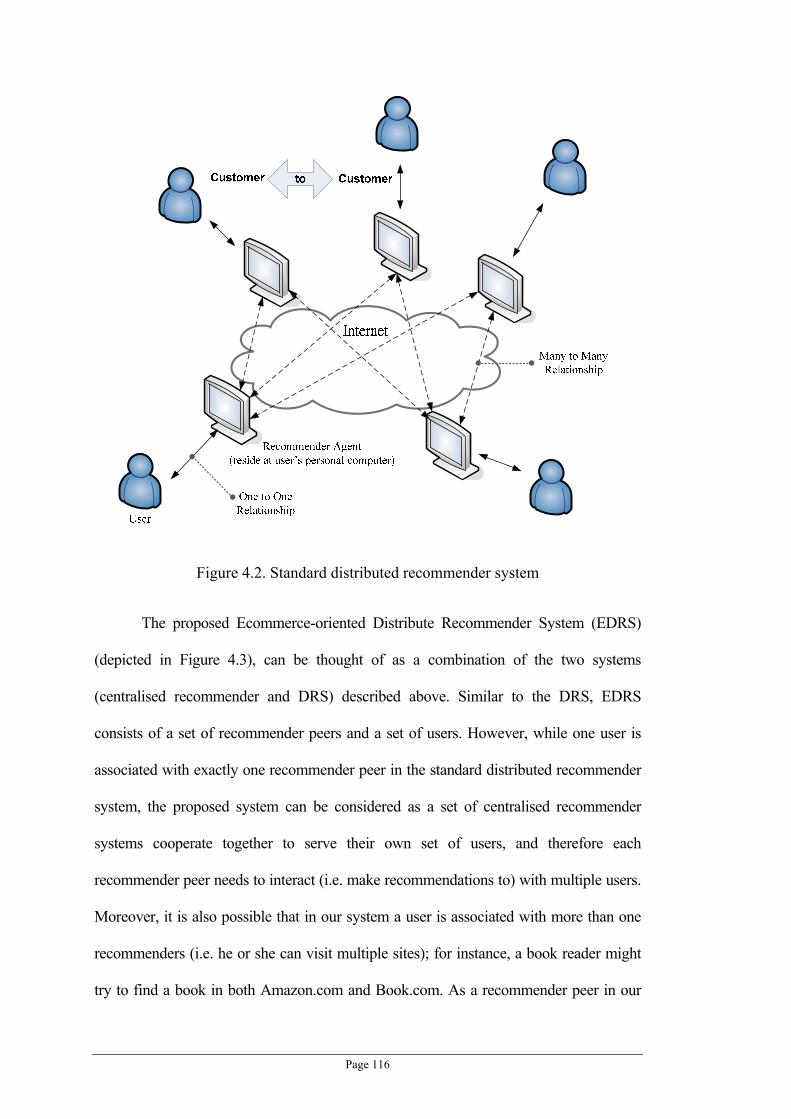
Page 116
Figure 4.2. Standard distributed recommender system
The proposed Ecommerce-oriented Distribute Recommender System (EDRS)
(depicted in Figure 4.3), can be thought of as a combination of the two systems
(centralised recommender and DRS) described above. Similar to the DRS, EDRS
consists of a set of recommender peers and a set of users. However, while one user is
associated with exactly one recommender peer in the standard distributed recommender
system, the proposed system can be considered as a set of centralised recommender
systems cooperate together to serve their own set of users, and therefore each
recommender peer needs to interact (i.e. make recommendations to) with multiple users.
Moreover, it is also possible that in our system a user is associated with more than one
recommenders (i.e. he or she can visit multiple sites); for instance, a book reader might
try to find a book in both Amazon.com and Book.com. As a recommender peer in our

Page 117
system can serve multiple users and a user can make recommendation requests to
multiple recommender peers, the relationship between users and recommender peers is
considered as Many-to-Many. As mentioned previously, the recommender peers in
EDRS might interact and cooperate with each other to improve their recommendation
quality, and hence, apart from the Many-to-Many relationship between users and
recommender peers, another Many-to-Many communication relationship exists among
the peers.
Since EDRS is still designed for normal ecommerce sites, such as e-book stores
like Amazon.com, its major ecommerce model is therefore the same as CRS, that is,
Business-to-Customer. Besides, since EDRS introduces additional communication and
cooperation for recommenders of different sites, it is expected that the cooperation of
these recommenders (also their sites) will confirm to the Business-to-Business based
model.
The implementation of the proposed EDRS involves both Peer-to-Peer and
Client-Server architectural styles. Client-Server architecture is employed to model a
recommender peer (i.e. the server) and its users (i.e. the clients). Similar to the
centralised recommender, the entire recommendation generation process is done by the
recommender situated at the server side, and the users make requests to the
recommender through thin clients such as web browsers. The architectural style for the
network among the recommender peers is modelled with Peer-to-Peer architecture. As
mentioned previously, Peer-to-Peer based architecture assumes that the peers are
independent and autonomous from each other, and especially they should be loosely
coupled. Such a definition is suitable for modelling the relationship between the
recommender peers’ host sites, as they are both logically and physically independent and
autonomous from each other (as they are different ecommerce sites and organisations).

Page 118
While both DRS and the proposed EDRS can be modelled with the Peer-to-Peer
architecture, the recommender peers in EDRS are more strongly coupled together than in
standard DRS. This is because the recommender peers in EDRS need to
gather/distributed information and suggestions from/to each other in a timely and
effective fashion to achieve their common goal (i.e. satisfy their users’ information and
recommendation needs).
To the best of our knowledge, the concept of the proposed EDRS has not yet
been mentioned and investigated by other studies. In addition, it is different from
existing recommender systems (both centralised and distributed ones) at several high
level aspects. Table 4.1 summarises these differences.
Table 4.1. High level aspect differences among recommender system paradigms
Ecommerce Model
Architectural Style Communication Paradigm
CRS B2C Client-Server One-to-Many (recommender to user)
DRS C2C Peer-to-Peer
Many-to-Many (recommender to recommender) One-to-One ( recommender to user)
EDRS B2C, B2B Client-Server, Peer-to-Peer
Many-to-Many (recommender to recommender/
Recommender to user)

Page 119
UserMany to ManyRelationship
Many to Many Relationship
Recommender Agent (reside at Ecommerce site’s server)
BusinessBusiness to
Customer
Business
to
Figure 4.3. Proposed distributed recommender system
4.2.1 General Interaction Protocol
As mentioned earlier, the interaction, communication and cooperation of the
recommender peers in the proposed EDRS can be modelled with the Peer-to-Peer based
architectural style. In particular, the ‘Contract Net Protocol’ (CNP) is employed as the
foundation for modelling the system, which provides the basis for coordinating the
interaction and communication among the recommender peers. Contract Net Protocol is
a high level communication protocol and system modelling strategy for Peer-to-Peer

Page 120
architectural based systems (or other distributed systems) (Smith, 1981, Weiss, 1999). In
CNP, peers in the distributed system are modelled as nodes and the collection of these
nodes is referred to as a contract net. In CNP based systems, the execution of a task is
dealt with as a contract between two nodes, each node plays a different role, one of them
is the manager role and the other is the contractor role. The role of a manager is
responsible for monitoring the execution of a task and processing the results of its
execution. On the other hand, the role of a contractor is responsible for the actual
execution of the task. It is important to note that the nodes are not designated a priori as
contractors or managers, rather, any nodes may take on either roles dynamically based
on the context of their interaction and task execution (Weiss, 1999, Smith, 1981). A
contract is established by a process of mutual selection based on a two-way transfer of
information. In general, available contractors evaluate task announcements made by
managers and submit bids on those for which they are suited. The managers evaluate the
bids and award contracts to the nodes (i.e. contractors) that they determine to be most
qualified (Smith, 1981).
In the case of the proposed EDRS, the recommender peers are modelled as the
nodes in the contract net. Depending on difference circumstances, each recommender
peer plays manager role and contractor role interchangeably. When a recommender peer
makes requests for recommendations to other peers, it is considered as a manager peer.
Conversely, the recommender peer that receives a request for recommendations and
provides recommendations to other peers is considered as a contractor peer. The roles of
the manager peer and the contractor peer and their interactions are depicted in Figure 4.4.

Page 121
Figure 4.4. High level interaction overview for EDRS (based on contract net protocol)
The communication steps involved in the interaction are indicated by the
numbers in Figure 4.4 and explained as follows:
(1) User sends a request for recommendations. The recommender peer who
received the request and is responsible for making the recommendation to
the user is considered to be in the manager role.
(2) Based on the user’s request and profile, the manager peer selects suitable
peer recommenders to help it on making better recommendations to the user.
(3) The manager peer makes requests to the peers for recommendation
suggestions. The request message may only contain the user’s item
preferences (i.e. the user’s rating data); however, the identity of the user is
anonymous for privacy protection.
(4) Each contractor peer generates recommendations based on the received
request.

Page 122
(5) The contractor peers send back their recommendation suggestions to the
manager peer.
(6) After the manager peer received the suggestions from the contractors, it then
synthesises and merges these recommendation suggestions.
(7) Based on the synthesised recommendation suggestions from the contractor
peers (might also include the manager peer’s own recommendations) the
manager peer generates the item recommendations to the user.
(8) When the user received the recommendations, he or she might supply
implicit or explicit ratings to the recommendations. That is, the user might
provide indications about whether he or she likes or dislikes one or more
items in the recommendation list.
(9) Based on the user rating feedbacks, the manager peer can objectively
evaluates each of the peers’ (i.e. contractors’) performances to the
recommendation suggestions they supplied and update its profiles about
these peers.
(10) The manager peer sends feedbacks and rewards to the contractor peers based
on their performances to the task.
(11) When the contractor peers received feedbacks about the performances of
their recommendation suggestions, they then update their profiles about the
manage peer in order to improve their future suggestions.
From Figure 4.4, it can be seen that when a recommender peer is requested to
make recommendations for a user, it acts as a manager peer. In the role of a manager
peer, the recommender first generates a strategy about how and what to recommend to
the user based on the user’s profile and request. Then the recommender chooses a set of
recommender peers (in this context, they act as contractor peer) based on the profiles of

Page 123
peer recommenders, and finally makes requests for recommendations to these selected
contractor peers. When these selected contractor peers received the requests, they then
construct and return their recommendation suggestions based on the requests received
and the manager peer’s profile (e.g. preferences, domain of interests, and
trustworthiness). After the manager peer received the recommendations returned from
the contractor peers, it then merges the recommendations (also include recommendations
from itself) and return to the user. According to the recommendations received from the
manager peer, the user might either explicitly or implicitly give feedbacks or ratings
about the recommendations to the manager peer. After receiving the user’s feedback, the
manager peer will evaluate the performance of each of the selected contractor peers,
update its profiles about them, and then construct the feedbacks and make rewards to the
contractor peers. Finally, the contractor peers will update theirs profile about the
manager peer based on the given rewards and feedbacks.
In order to carry out the proposed interaction described above, the following
tasks need to be considered.
Recommender Peer Selection: After a manager peer received a request
from a user, it needs to determine a subset of recommender peers from all
available recommender peers to consult for recommendations. A mechanism
is required so that:
(1) The number of peers selected is minimised (to ensure efficiency); and
(2) The user’s satisfaction to the collected recommendations is maximised.
Recommendation generation: As the system is loosely coupled (as these
recommender peers are from different ecommerce sites), therefore, each
peer does not hold detailed knowledge about the data collections, the
operations and functions of other peers. Hence, depending only on the

Page 124
request sent from the manager peer is not sufficient for the contractor peers
to generate quality recommendations. Therefore, the contractor peers
generate recommendations based on both the content of the request and their
profiles about the manager peer as well.
Recommendation merge: Mechanisms are required for the manager peer
to synthesise the recommendation gathered from different contractor peers,
such that:
(1) The synthesised recommendation should result in a high level
satisfaction from the target user. In general, the synthesised
recommendation should have better quality than the recommendation
generated by the manager peer itself; and
(2) The contributions of the contractor peers to the synthesised
recommendation need to be balanced (i.e. without degrading the quality
of the recommendation, the final recommendation should be constructed
by considering as many contractors’ recommendations as possible), so
that the manager peer can extend or update its knowledge to as many
peers as possible based on the user feedbacks to the recommendation.
Peer feedback and profile update: The major source that recommenders
can learn about each other is from the user feedbacks. Based on the user
feedbacks to a particular recommendation, the manager peer needs to
evaluate the performances of each individual contractor peer, and further
acquire better understanding about them. Moreover, the manager peer also
needs to supply feedbacks and rewards to the contractor peers, so that the
contractor peers can learn the manager peer’s preferences as well.

Page 125
Hence, it can be observed that each of the recommender peers in the EDRS
need to maintain two set of peer profiles. The first set of profiles is the
contractor peer profile set which is used when the peer is in the manager role
and other peers are in contractor role. In contrast, the second set of profiles is
the manager peer profile set which is used when the peer is in the contractor
role and other peers are in manager role. However, due to the limited scope
of this thesis, only the contractor peer profiles are considered in our thesis
and experiments. Thus, we allow a recommender peer in the manager role to
select other contractor peers based on its contractor peer profile set, and as
the contractor peers maintain no profiles about the manager peer, it is
assumed that they will generate recommendations to the manager peer only
based on the manager peer’s current request/query and not past behaviours.
Therefore, given two different manager peers with same requests, a
contractor peer will generate same recommendations to them.
Among these four proposed tasks mentioned above, recommender peer
profiling and selection for manager peers is the major focus of this thesis, and a novel
contractor peer profiling and selection strategy is proposed, discussed and investigated in
Section 4.3. Section 4.4 describes a simple technique for a manager peer to merge
recommendations generated from multiple contractor peers to form a single
recommendation to the target users. Due to the limited thesis scope, the strategy required
for contractor peers to profile manager peers are not included in this thesis.
4.3 PEER PROFILING AND SELECTION
Part of the major contributions in this chapter includes a recommender profiling
scheme (for manager peers to profile contractor peers) and a recommender selection

Page 126
algorithm designed for the proposed EDRS. In particular, the recommender peer
selection problem is modelled as the classical exploitation vs. exploration (or k-armed
bandit) problem (Azoulay-Schwartz et al., 2004, John, 1989), in which the recommender
selection for the manager peer has to be balanced between choosing the best known
contractor peers to keep users satisfied and selecting other unfamiliar contractor peers to
obtain knowledge about them. The proposed recommender selection algorithm is based
on evaluating the Gittins Indices (John, 1989) for every recommender peer, and the
indices reflect the average performance, stability and selection frequency of the
recommenders (i.e. contractor peers).
4.3.1 System Formalisation for EDRS
Before explaining the proposed strategies and techniques in detail, a formalised
description of the proposed EDRS is given below.
Similar to the formalisation used in Section 3.2.1, the set of users and items are
denoted by , , … , and , , … , respectively. The proposed
distributed recommender system (EDRS) denoted as Φ contains a set of recommender
peers , , … , , i.e. Φ , , … , . The number of recommender peers is
much smaller than the number of users in our system, i.e. . Each recommender
peer Φ has a set of users denoted as , and a set of items denoted as ,
where
and

Page 127
Moreover, as mentioned previously, some users and items can be owned by more
than one recommender peers such that
and
4.3.2 User Clustering
Intuitively, a large set of users can be separated into a number of clusters based
on the user preferences. Users within the same cluster usually share similar tastes
(Drineas et al., 2002) and a cluster with a large number of users and a high degree of
intra-similarity can better reflect the potential preferences of the users belonging to the
cluster. Thus, a collaborative filtering based recommender can improve its
recommendation quality by searching similar users within clusters rather than the whole
user set (Sarwar et al., 2002, Degemmis et al., 2004). However, different user clusters
often vary in quality. The performance of such clustering based collaborative filtering
system is strongly influenced by the quality of the clusters (Sarwar et al., 2002,
Degemmis et al., 2004). For a given recommender, some users might be able to receive
better recommendations if they belong to a cluster with better quality (the cluster has a
large number of users and a high intra-similarity), whereas some other users may not be
able to get constructive recommendations because the cluster to which they belong is
small and has a low intra-similarity. This situation is closely related to the cold-start
problem (Schein et al., 2002), which occurs when a recommender makes
recommendations based on insufficient data resources. Therefore, even for the same

Page 128
recommender, the recommendation performance might be different for different clusters
of users if different user clusters have different quality. In order to provide good
recommendations to various users, the proposed EDRS allows its recommender peers
(i.e. manager peers) to choose peers (i.e. contractor peers) for recommendations to the
current user based on their performances to a particular user cluster to which the current
user belongs. We expect this design to solve the cold-start problem because a
recommender that is making recommendations to a user who belongs to a weak cluster
can get recommendations from recommender peers who have performed well to that
group of users.
In the proposed EDRS, every recommender peer has its own set of user clusters,
and we denote the set of user clusters owned by Φ as
, , , , … , , , such that , . In addition, for the simplicity of the
system, all user clusters are assumed to be crisp sets, such that , , for
, , , , . As different recommender peers have different user sets and
different clustering techniques, the size of their cluster set might vary as well, that is,
, Φ: | | | | (or ).
4.3.3 Recommender Peer Profiling
In this section, we present our approach to profile the recommender peers within
the proposed EDRS. To begin with, the performance evaluation of the recommender
peers is explained. The performance of a recommender peer is measured by the degree
of user satisfactory to the recommendations made by the recommender (Herlocker et al.,
2004, Karypis, 2001, Papagelis and Plexousakis, 2004). In our system, a recommender
peer makes recommendations to a user with a set of items , , , , … , ,
where . Once having received the recommendations, the user then inputs his or

Page 129
her evaluations to each of the items. We use to denote the user’s rating to item
, . The value of is between 1 and 0 which indicates how much the user likes
item , . When closes to 1, it indicates the user highly prefers the item, in contrast
when closes to 0, the user dislikes the item. Hence, each time a recommender peer
generates a recommendation list (e.g. ) to a user, it will get feedback
, … , from the user, where 0,1 . With , we can compute the
recommender peer’s current performance χ to the user by:
∑| |
(4.1)
Equation (4.1) measures the current performance of a recommender peer to a
particular user in the current recommendation round. We can use the average
performance of the recommender to the users in the same cluster to measure its
performance to this group of users. The average performance measures how well the
recommender averagely performed in the past. However, the average performance does
not reflect whether the recommender is generally reliable or not. Hence, we employed
the standard deviation to measure the stability of the recommender. Another factor that
should be taken into account for profiling a recommender is the selection frequency,
which indicates how often the recommender has been selected before. In our system, we
profile each recommender peer from the three aspects: recommendation performance,
stability, and selection frequency. As mentioned previously in this chapter, a
recommender will seek for recommendations from other peers when it receives a request
from a user. Broadcasting the user request to all peers is one solution, but obviously, it is
not a good solution since not all of the peers are able to provide high quality

Page 130
recommendations. In EDRS, the recommender peers (i.e. manager peers) will select the
most suitable peers (i.e. contractor peers) for recommendations based on their profiles.
Therefore, each recommender peers in EDRS keeps profiles to each of the other
recommender peers.
A recommender peer may perform differently to different user clusters.
Therefore, its performances to different user clusters are different. For recommender
Φ which has user clusters, that is, , , , , … , , we use , to
denote the average performance of peer Φ to ’s user cluster , . Hence, we can
use a matrix , to represent the average performance of each of the
other peers to each of ’s user clusters, where |Φ| 1 and | | . is
called as the peer average performance matrix of . Similarly, we use and to
represent the stability and selection frequency of other peers to . , and
, are called as the peer stability matrix and peer selection frequency matrix
respectively. In summary, a recommender ’s peer profile is defined as
, , which consists of the three matrixes representing peer recommender’s
average performance, stability, and selection frequency, respectively.
Initially, the , and of are all zero matrixes, because has no
knowledge about other peers. These matrixes will be updated when a recommender peer
helped (i.e. is in contractor role and is in manager role) to make a
recommendation for a user belonging to (or being classified to) a ’s user cluster
, . Suppose that is the recommendation list returned by . Ideally, is expected
to b a subset of . But usually since and may have different item sets. In
the proposed EDRS, only the items that are in are considered by . Let be the final
recommendation list made by to the user and

Page 131
| and selected by be the recommendation list made by and
selected by during the merging process (the major focus of this selection is on peer
profiling, other aspects of the proposed EDRS such as merging recommendations from
different peers will be explained in latter sections). should be a subset of . After the
recommendation is provided to the user, will get a feedback list (i.e. the actual user
ratings to the recommended items) about from the target user. With the user
feedback , Equation (4.1) will be used to compute ’s performance for the
recommendation of this round (only the items in are taken into consideration when
compute the for ) which is ’s observation about ’s performance to user cluster
, . The methods for updating the average quality, stability and selection frequency in
’s peer profile , , are given below, where , , , , , are the updated
value for peer and cluster , in the three matrixes, respectively:
,, ,
, 1
(4.2)
, , 1
(4.3)
,
0, , 2
, 1 ,
,
χ ,
, 1,
(4.4)

Page 132
Equation (4.2), (4.3) and (4.4) simply keep track of the average and standard-
deviation of the recommender performances as well as the number of times the
recommender peers were selected (for a user cluster). In the next section, we will
describe the proposed recommender selection approach based on these three matrixes.
4.3.4 Recommender Peer Selection
In this section, a novel technique is proposed that allows manager peers to
effectively and efficiently select contractor peers based on the proposed recommender
peer profiles described in Section 4.3.3 for assistances in making quality
recommendations. The proposed peer selection strategy is based on the famous Gittins
Indices technique (John, 1989) developed for solving the exploitation vs. exploration
problem, as such, it enables the manager peers to efficiently learn their contractor peers
as well as maintain their recommendation quality to the users.
4.3.4.1 Gittins Indices
In this section, a brief explanation of the Gittins indices is given. The Gittins
indices (John, 1989) is developed for the -armed bandit problem (which is a subset of
the exploitation vs. exploration problem) that deals with a slot machine with k arms. An
amount of reward will be given when an arm is pulled. However, in each period, only a
limited number of arms can be pulled (normally one arm). Different arms have different
reward distributions, and the reward distributions for the arms are initially unknown. The
objective is to choose which arms to pull that will maximise the total rewards over time
based on previous experience and obtained rewards. Formally, the k-armed bandit
problem is to schedule a sequence of pulls maximising the expected present values of

Page 133
(4.5)
where indicates the time points, denotes the sum of the rewards obtained by
pulling a set of arms at , and is a fixed discount factor where 0 1.
Traditionally, dynamic programming was the preferred framework for solving
the bandit problem. It requires analysis of all possible combinations of the pulling
sequences. However, Gittins developed a solution in 1972 that required computation
only on the current states of the individual arms. Gittins suggests comparing each
potential action (i.e. a pull) against a reference arm with a known and constant reward¸
instead of to compare all possible actions against each other (John, 1989). Gittins proved
it is optimal to select actions with expected rewards equal to the reference actions with
the highest equivalent rewards (i.e. Gittins index values) for each pull (John, 1989).
Specifically, a Gittins index value of an arm is computed based on the average
and standard deviation of the rewards generated from the arm as well as the number of
times the arm has been pulled. The application of the Gittins indices for solving the
multi-armed bandit problem is therefore straight forward: we simply compute the Gittins
index values for every arms (based on their current average and standard deviation of the
rewards generated and the number of times each of them are pulled), and pull the arm
with the highest index value. As the arm selection task involves only the current states
of the arms (i.e. current average and standard deviation of the rewards and number of the
times being pulled), it is, therefore, both memory and computationally efficient (when
comparing to dynamic programming based solutions).

Page 134
The theorem background and the relevant index value generation techniques of
the Gittins Indices technique are detailed in (John, 1989). This thesis mainly focuses on
the application of the Gittins indices in the context of the recommender peer selection
task. In this thesis, we employed one of the Gittins methods to generate the index values
based on the multi-population sampling in relation to the mean and standard deviation
rewards of the arms. For a given discount factor , the Gittins indices can be calculated
by back-solving the recurrence relation:
, , , 1
, , , , 1 | , ,
(4.6)
where is the current number of trials, is the average rewards generated from
past trials, and is the standard deviation of the rewards. is the updated average
rewards giving is the new reward generated by the distributions function | , ,
in the 1 trial, such that
1
and denotes the updated standard deviation of the 1 rewards
1 1
Generally, Equation (4.6) expresses the selection between a referenced arm
with a constant reward and an uncertain arm with an expected reward . In the
Equation (4.6), the term
, , , 1 | , ,
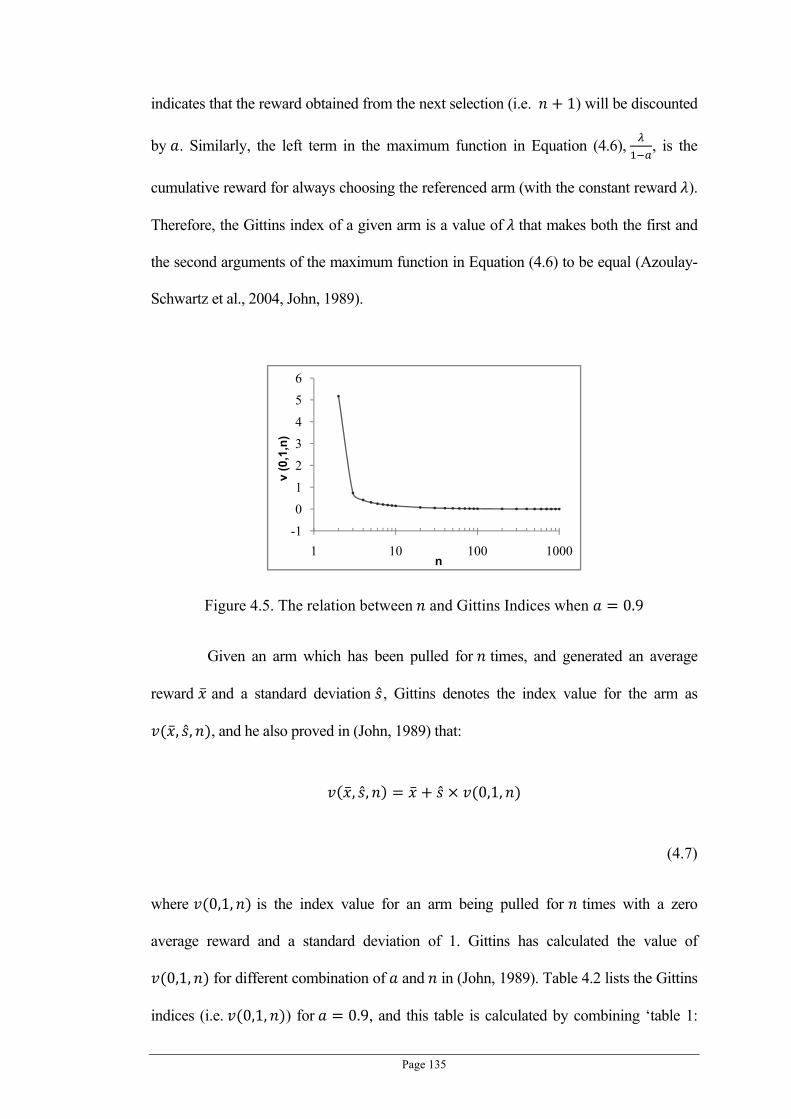
Page 135
indicates that the reward obtained from the next selection (i.e. 1) will be discounted
by . Similarly, the left term in the maximum function in Equation (4.6), , is the
cumulative reward for always choosing the referenced arm (with the constant reward ).
Therefore, the Gittins index of a given arm is a value of that makes both the first and
the second arguments of the maximum function in Equation (4.6) to be equal (Azoulay-
Schwartz et al., 2004, John, 1989).
Figure 4.5. The relation between and Gittins Indices when 0.9
Given an arm which has been pulled for times, and generated an average
reward and a standard deviation , Gittins denotes the index value for the arm as
, , , and he also proved in (John, 1989) that:
, , 0,1,
(4.7)
where 0,1, is the index value for an arm being pulled for times with a zero
average reward and a standard deviation of 1. Gittins has calculated the value of
0,1, for different combination of and in (John, 1989). Table 4.2 lists the Gittins
indices (i.e. 0,1, ) for 0.9, and this table is calculated by combining ‘table 1:
-1
0
1
2
3
4
5
6
1 10 100 1000
v (0
,1,n
)
n

Page 136
normal reward process with a known variance’ and ‘table 3: the ratio of indices for cases
of unknown variance and known variance’ in the appendix of (John, 1989). We also
illustrate the relation between and 0,1, in Figure 4.5, which is portrayed based on
the Table 4.2.
Table 4.2. The Gittins indices table for 0.9
0,1, 0,1, 0,1,
2 5.169212 20 0.074436 200 0.007931
3 0.735712 30 0.050491 300 0.005307
4 0.416059 40 0.038287 400 0.003988
5 0.30622 50 0.03086 500 0.003194
6 0.246668 60 0.025856 600 0.002664
7 0.208662 70 0.022254 700 0.002285
8 0.181654 80 0.019534 800 0.002
9 0.161279 90 0.017409 900 0.001778
10 0.144795 100 0.015701 1000 0.001601
Based on Equation (4.7), it can be observed that as an arm’s average rewards
increases, its index value increases too. Moreover, despite the average rewards, the
standard deviation of the arm’s past performances and the number of times the arm has
been pulled also play important roles in the index calculation. It can be seen from Figure
4.5 that the standard index value 0,1, is only significant when is small (i.e.
3 ), when gets bigger, 0,1, shrinks. By combining 0,1, with as
shown in Equation (4.7), the contribution of the standard deviation of an arm’s past
rewards to the index value , , decreases drastically when increases. Intuitively,
Equation (4.7) indicates that when our experience to an arm is low (i.e. is small) it is
better to select the arm if it is highly risky (i.e. if is higher), because the risky arm

Page 137
might potentially generate high rewards in the future. In contrast, if we already have a
long experience with the arm, then it would be more important to look at the arm’s
average rewards rather than to gamble on its instability.
The above concepts can be adapted into the recommender peer selection problem.
Recommender peers can be treated as the arms in the armed bandit problem. The
number of times a recommender has been chosen corresponds to the number of times an
arm has been pulled. The calculations for and are the same to the profile
updating to the average and the standard deviation of the recommender peer
performance (i.e. Equation (4.2) and Equation (4.4)). Initially, if a recommender peer (i.e.
manager peer) does not know about other peers (i.e. contractor peer) very well (i.e. low
values in the selection frequency matrix), then it would be a good strategy to select peers
with lower stability, because the unstable peers might become better in the future
(whereas stable peers stay unchanged). However, after a certain period, the stability of
the peers becomes insignificant, because as the number of trials increases the average
performance of the peers become reliable and dominate over the stability.
4.3.4.2 Selection Strategy for EDRS
Based on Section 4.3.4.1, when a manager peer wants to find a best
contractor peer to make a recommendation to a user , where , Φ and
, , the following equation is used to select the most suitable peer:
argmax\
, , ,
(4.8)

Page 138
where , is the Gittins index function that maps , (i.e. selection frequency) to the
corresponding 0,1, , based on Table 4.2. In Equation (4.8), firstly calculates the
average performance, stability and selection frequency of the available peers to the user
cluster that belongs to (i.e. , ). Then computes the index values for every peer
based on Equation (4.7). Finally, the most preferred peer will be the one that has the
highest index value. By setting up a cut-off for the index value, multiple recommender
peers with index values higher than the cut-off can be selected. However, selecting
multiple peers to make a recommendation requires recommendation fusion that will be
briefly discussed in latter sections. In addition, the discount factor as depicted in
Equation (4.5) and (4.6) discounts the future rewords exponentially, this implies that it is
more important for a recommender to achieve higher performance in the present rather
than to achieve the same performance in the future. Therefore, the smaller the value of ,
the severer the future rewards are discounted. In this thesis, we suggest a large value for
(i.e. 0.9) which discounts the future rewards in a gentle fashion, because we
perceive that the long term relationships between the recommenders are necessary.
4.3.4.3 An Example
In this section, an example is provided to demonstrate the proposed
recommender peer selection method. We start by assuming that a recommender
(manager peer) has made recommendations to a user in cluster , by consulting
four contractor peers , , and before, the past performances of the
recommender peers are computed based on Equation (4.1) and are given in Table 4.3,
where the number of times that , , and are selected to make recommendation.

Page 139
Table 4.3. Performance histories for four recommender peers
Peers Rewards (χ) Received
0.2, 0.6, 0.3
0.3, 0.45, 0.42
0.9, 0.4, 0.8, 0.6
0.7, 0.7, 0.8, 0.75, 0.68, 0.8
Given , as the user cluster, ’s profiles to the peers are three 4-dimension
column vectors:
0.3667, 0.39, 0.675, 0.7383
0.2082, 0.0794, 0.2217, 0.0531
3, 3, 4, 6
Apparently, ’s profile vector is the elements of the vectors, that is , , , ,
, . The vectors are calculated by applying Equation (4.2), (4.3) and (4.4) to Table 4.3.
In order to calculate the Gittins indices for the recommender peers, we have to convert
into standard Gittins indices as described in Section 4.3.4.2:
0.735712, 0.735712, 0.416059, 0.246668
The conversion from to is simply a table lookup to Table 4.2. Next, we
compute the intended Gittins indices vector, , by combining , and based
on Equation (4.7):
0.5918, 0.4484, 0.7673, 0.7514
where denotes element-wise multiplication.
If only the past performances of the recommender peers are considered, is the
best choice because it performed best (i.e. , max 0.7383) in the past.

Page 140
However, based on , it suggests that is the best choice. We can better understand
the rationale behind the choice by comparing the stability between and . Even
though averagely performed better than (i.e. , , ), it is still worthwhile to
take risk on , because has only been selected for 4 times and its performances
varied drastically ( , 0.2217). might be a still a good choice (with the second
highest index , 0.7514), however, because it is already relatively stable ( ,
0.0531), we can take chance to learn more about other peers first. Therefore, is
preferred to . The same concept can be applied when comparing with . With the
same selection frequency ( , , 3), although generally outperforms , it is
suggested to take risk on the unstable peer , as it might potentially improves its
performance.
4.4 RECOMMENDATION MERGE
Recommendation merge is an important task for distributed recommender
systems, but it is not a key focus of this thesis due to time limitations. In this section, we
present a simple technique for a manager peer to merge recommendations generated
from a set of contractor peers. Here, we assume the set of contractor peers is selected
based on the peer profiling and selection strategy described in Section 4.3, and therefore,
each of these selected peer will be associated with a Gittins score (see Section 4.3.4.2)
that indicates the expected utility the manager peer might obtain when the contractor
peer’s recommendation is adopted.
In the recommendation merge task, a manager peer selects top contractor
peers Φ , , . . with the highest Gittins scores for recommendation
suggestions, and each of these selected contractor peers Φ sends the manager peer

Page 141
a recommendation list , , , , , , , , … , , , , . As discussed in
Section 4.3.3, only items that are in are considered by . Therefore, after removing
the items from which are not in , for each value pair , , , in , , is
the recommended item and , 0,1 indicates ’s confidence that , will be
preferred by the manager peer’s target user. Note, because different recommender peers
might have different recommendation methods, so their confidence scores (i.e. , )
might not be directly comparable to each other. For simplicity, we assume that the
confidence scores from different recommender peers are normalised and comparable, so
that if the scores , and , of two peers , Φ to items , and , are
similar (i.e. , , ), the two peers have similar confidences to the two items.
Let , , … , be the set of items each of which is recommended by at
least one of the contractor peers, i.e. the items in , must appear at least in one of the
recommended lists , , , , , , … , , , , 1, . . . If 'ppi was
not recommended by contractor , then , 0 . Merging the recommended lists
returned from contractors , , . . can be viewed as to recalculate the scores to the
items in , based on the scores given by the contractors. Let
, , , , … , , be the final recommendation list after merging the
recommended lists , , , , , , … , , , , 1, . . , to merge the
recommendations is to calculate the scores based on , , 1, . . , 1, . . .
As the contractor peers Φ are selected by manager peer based on the
Gittins scores, therefore, each is associated with a corresponding Gittins score ,
(see Section 4.3.4.2 and Section 4.3.4.3 for detailed Gittins score computation). Note,
the symbol , is borrowed directly from Section 4.3.4.3, where indicates , , the
target user’s belonging cluster in . We propose to use a linear combination of the

Page 142
contractor peers’ Gittins scores ( , ) and the recommendation scores (i.e. , ) they
assigned to the items to calculate the final score to the items. The algorithm to perform
the merging is given below:
Algorithm 4.1 _ ,
Input , , , , … , is the set of Gittins scores for the selected
contractor peers. , denotes the Gittins score the manager peer assigned
to the contractor peer Φ for its recommendation to the target user in
, .
, , … is the set of recommendation lists generated from the
selected recommender peers. denotes the recommendation generated by
the contractor peer Φ to the manager peer .
Output is the merged recommendation list
1) SET , , an initially empty set for storing all items involved in
2) FOR EACH
3) FOR EACH , , ,
4) SET , ,,
5) END FOR
6) END FOR
7) SET , an initially empty set for storing the final merged recommendation
list
8) FOR EACH ,
9) SET 0, 0
10) FOR EACH

Page 143
11) SET , ,
12) IF , 0 THEN ,
13) END FOR
14) SET /
15) SET ,
16) END FOR
17) Return as the merged recommendation list
In Algorithm 4.1, the manager peer firstly finds all items that are
recommended by the contractor peers (i.e. from line 1 to line 6) and stores them in the
candidate item set ,. As it is possible that different contractor peers may suggest the
same items in their recommendation lists, the size of , the candidate item set is,
therefore, between the size of the largest recommendation list (in the case that all
contractor peers recommend the same set of items) and the size of the union of all
recommendation lists (in the case that all contractor peers recommend different items),
specifically:
max | | | ,| | |
In Algorithm 4.1, the linear combination of the Gittins scores and the
recommendation item scores is implemented from line 10 to 13. Line 11 indicates that
the item scores received from the contractor peers are factored by the peers’ Gittins
scores. Thus, items suggested by the contractor peers with higher Gittins scores will
receive high final scores. Moreover, in line 14 of Algorithm 4.1, is normalised by the
sum of the Gittins scores of the contractor peers who have recommended the item.

Page 144
4.5 EXPERIMENTS AND EVALUATION
As mentioned in the beginning of this chapter, the major objective of the research
presented in this chapter is to demonstrate the possibility of alleviating the cold-start
problem by enriching the information resources with help from recommenders of other
parties. Specifically, we proposed an EDRS framework (see Section 4.2) for modelling
the interactions and communications of the recommenders, and the goal of the
framework is to allow the recommenders to improve their recommendation quality by
integrating their recommendations together. In order to facilitate the interaction protocol
of the proposed EDRS, in Section 4.3 we proposed a recommender peer profiling and
selection technique which allows recommenders to effectively learn from each other and
select the partner recommenders that can help them best. Based on the goals we
presented in this chapter, the experiments we conducted in this part of thesis aim to
verify the following:
Whether recommenders can improve their recommendation quality as well
as their resistance to the cold-start problem by incorporating aid from
recommenders of other organisations.
Whether the proposed peer profiling and selection strategy can effectively
facilitate the interactions of the recommender peers within the proposed
EDRS framework.
In this experimentation, multiple recommenders with different capability in
making recommendations are constructed, and we allow them to interact with each other
based on the proposed EDRS framework. Essentially, these recommenders employ the
proposed peer profiling and selection strategy presented in Section 4.3 to learn from and
select each other in order to improve their recommendation making. Our main focus is to
examine whether incorporating aid from other recommenders can indeed improve

Page 145
recommenders’ recommendation quality and also to evaluate the effectiveness of the
proposed profiling and selection strategy.
Note, due to the limited scope of this thesis and also the recommendation merge
is not a key focus of this thesis, the experiment is configured such that the manager peers
select only one contractor peer for each recommendation making round, and the
manager peer forward directly the recommendations from the selected contractor peer to
the target user. Hence, the recommendation merge technique described in Section 4.4 is
not involved in this experiment. However, as the peer profiling and selection strategy is
the most essential part of the proposed EDRS framework, our experiments sufficiently
cover the two previously mentioned experimentation goals.
In Section 4.5.1, the dataset we employed for the experiments is discussed. In
Section 4.5.2, the experiment process and settings used for evaluating the proposed peer
profiling and selection technique are discussed. Finally, in Section 4.5.3 the experimental
results are presented and explained.
4.5.1 Data Acquisition
The dataset employed in this experiment is the ‘Book-Crossing’ dataset
(http://www.informatik.uni-freiburg.de/~cziegler/BX/) which is also the main
experiment dataset employed in Chapter 3. Please refer to Section 3.3.1 for more details
about the dataset.
As this experiment involves only the standard item-based collaborative filtering
recommender, the product taxonomy data employed in Chapter 3 is not used in this
experiment.

Page 146
4.5.2 Experiment Setup
As the main purpose of this experiment is to evaluate the proposed interaction
protocol and the peer profiling and selection technique (rather than evaluating a new
recommendation technique or algorithm) in a distributed recommender system, therefore,
the overall setup of this experiment is different from the setup for non-distributed
recommender systems.
In this experiment, it is required to simulate the interactions (i.e. profiling and
selection) among the recommenders from different organisations, and therefore the first
step in the experiment setup process is to construct multiple recommenders with
different capabilities and underlying knowledgebase (i.e. datasets). Next, the testing
dataset is constructed for evaluating the recommenders’ recommendation quality.
Importantly, the recommendation quality comparison between recommenders utilising
the proposed EDRS framework (i.e. getting aid from other recommenders) and stand-
alone recommenders (i.e. making recommendations based on their own efforts) are
carried out. Moreover, the effectiveness of the proposed peer profiling and selection
technique is also examined by comparing it with other peer selection strategies. Note, the
proposed peer profiling strategy requires the manager peers to get user feedbacks for all
of their recommendations (see Section 4.3.3) so they can determine their contractor peers
performances based on the feedbacks and then update their peer profiles. Hence, it is
necessary to provide a way to allow the user feedbacks in the experiment. The tasks
involved in this experiment setup are detailed in the following subsections.
4.5.2.1 Constructing the Recommender Peers
In this experiment, four recommenders of different organisations are constructed
to simulate the proposed recommender peer interactions. These four recommenders are

Page 147
named as ORG1, ORG2, ORG3 and ORG4, and they are equipped with different
datasets but use the same underlying recommendation technique.
By evaluating the performances of the recommenders with the same
recommendation technique and different underlying datasets, we can evaluate the
performance of the recommenders based on their available information resources (i.e.
their underlying datasets and collaboration from other recommender peers) without the
impact from using different recommendation techniques. Moreover, the results from the
experiments can also be used to verify the proposed solution to the cold-start problem
(i.e. enriching the information resources from other parties).
The recommendation technique employed by the four recommenders is the
standard item-based collaborative filtering technique that is identical to the benchmark
recommender IR employed in Chapter 3 (see Section 3.3.3.1 and Section 2.1.2.1 for
more details). The use of the state-of-the-art recommendation technique ensures that our
experiment can be compared and verified with other studies. Moreover, it also suggested
that the proposed EDRS framework and peer profiling and selection strategy can be
easily adopted by existing recommenders.
The main differences among the four recommenders are in their underlying
datasets, specifically, they all have different customer sets (or user sets). We firstly select
6500 users from the Book-Crossing Dataset and then cluster them into 20 user clusters
based on their item preferences (i.e. explicit item ratings). We denote the overall user set
as and the 20 user clusters as , , … , . Specifically, | | 6500 ,
and .
From these 6500 users in , 5000 users are selected as the training user set
(i.e. for forming the underlying datasets of the recommender peers) and the rest of 1500
users then forms the testing user set , where and . Furthermore,

Page 148
we denote the set of training users within cluster as (i.e. ), the set
of testing users within cluster as (i.e. ), and .
Importantly, the users in are divided into the clusters first, and the 1500 users in the
testing set are then selected from each of the clusters. This process allows us to keep
track of the percentages of the different user types (i.e. users in different clusters) in the
testing user set. The allocation details for are shown in Table 4.4. Specifically, each
row in Table 4.4 shows the user allocation detail for a cluster. For example, the first row
in the table shows that there are totally 2278 users being grouped into among which
300 users are selected into the testing user set (i.e. | | 300). Note, because the size
of clusters , , , and , we do not select any users from them into the
testing set.
Next, the datasets for the four recommender peers ORG1, ORG2, ORG3 and
ORG4 are constructed from , and they are denoted as , , , and respectively.
As mentioned in Section 4.2, the users and recommender peers in the proposed EDRS
are in many-to-many relation, thus, it is possible that a user can exist in multiple
recommenders’ datasets (i.e. ). Table 4.5 shows the detailed
allocations for the datasets of the four recommenders. The four recommenders are each
having different user set sizes, ORG1 has the largest dataset with 2000 users, ORG4 has
the smallest dataset with 700 users, and ORG2 and ORG3 both have 1250 users in their
datasets. Even the total number of users involved in the four user sets is 5200 according
to Table 4.5, the total number of users involved in these four recommenders is actually
equal or smaller than 5000 (i.e. ) due to the user overlapping
allowed among the datasets. Moreover, it is shown in that different recommenders have
different numbers of users in different clusters, for example, ORG1 has the highest
number of users in (i.e. | | 1500) whereas ORG3 has the highest number
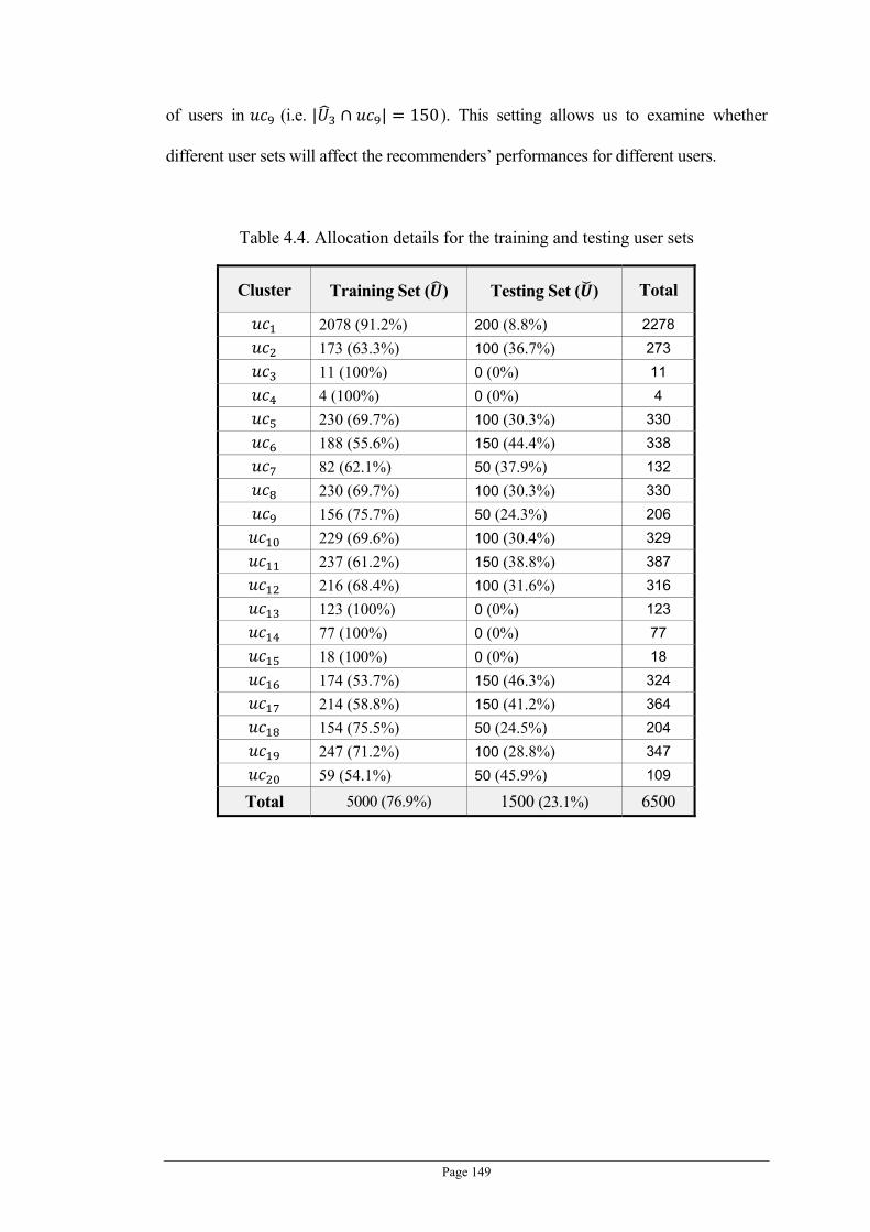
Page 149
of users in (i.e. | | 150). This setting allows us to examine whether
different user sets will affect the recommenders’ performances for different users.
Table 4.4. Allocation details for the training and testing user sets
Cluster Training Set ( ) Testing Set ( ) Total
2078 (91.2%) 200 (8.8%) 2278
173 (63.3%) 100 (36.7%) 273
11 (100%) 0 (0%) 11
4 (100%) 0 (0%) 4
230 (69.7%) 100 (30.3%) 330
188 (55.6%) 150 (44.4%) 338
82 (62.1%) 50 (37.9%) 132
230 (69.7%) 100 (30.3%) 330
156 (75.7%) 50 (24.3%) 206
229 (69.6%) 100 (30.4%) 329
237 (61.2%) 150 (38.8%) 387
216 (68.4%) 100 (31.6%) 316
123 (100%) 0 (0%) 123
77 (100%) 0 (0%) 77
18 (100%) 0 (0%) 18
174 (53.7%) 150 (46.3%) 324
214 (58.8%) 150 (41.2%) 364
154 (75.5%) 50 (24.5%) 204
247 (71.2%) 100 (28.8%) 347
59 (54.1%) 50 (45.9%) 109
Total 5000 (76.9%) 1500 (23.1%) 6500

Page 150
Table 4.5. Dataset allocation details for the four recommender peers
Cluster ORG 1 ( ) ORG 2 ( ) ORG 3 ( ) ORG 4 ( )
1500 500 250 0
100 100 0 0
0 0 0 0
0 0 0 0
10 150 0 200
90 100 0 0
0 0 0 50
30 0 0 0
0 50 150 0
0 0 0 200
0 150 0 200
100 0 200 0
0 0 0 0
0 0 0 0
0 0 0 0
60 0 250 0
60 0 250 0
0 0 150 0
50 200 0 0
0 0 0 50
Total 2000 1250 1250 700

Page 151
4.5.2.2 Evaluation Metrics
The classification accuracy metrics (i.e. Precision, Recall and F1 metrics) are
chosen for the performance evaluation of the recommenders against the users in the
testing user set. As these metrics have also been used for the experiments in Chapter 3,
please refer to Section 3.3.3.3 for detailed explanations to these metrics.
As described in Section 2.4 and Section 3.3.3.3, the classification accuracy
metrics are mainly based on comparing the recommended item list and the set of user
preferred items. In this experiment, for each testing user , we divide the set of
items explicitly rated by (denoted as , where T) into two halves denoted by
and , where , and | | | |. As all of the items in are
explicitly rated by , therefore, for any item , is associated with a numeric
item rating , 0,1 . For the two item sets , , and the associated item
ratings are used to represent ’s user profile (i.e. the recommenders make
recommendations to based on ’s ratings to the items in ), and the items in ,
conversely, are used to form the user preferred item list for evaluating the
recommendations made to . However, not all the items in are preferred by the user
. The items with low rating values should not be considered as the user’s preferred
items because has specifically indicated that they are disliked. Hence, the final testing
item set is constructed by removing all items with ratings below ’s average rating
from .
For evaluating the recommenders’ recommendation quality to a given testing
user , the recommenders are firstly provided with ’s profile (i.e. and the
associated ratings), then the recommenders generate their recommendations to , finally,

Page 152
the recommendations generated from the recommenders are evaluated against the testing
item set by utilising the classification accuracy metrics (i.e. Precision, Recall and F1).
4.5.2.3 Benchmarks for the Peer Profiling and Selection Strategy
As mentioned earlier, one of the objectives of this experiment is to evaluate the
effectiveness of the proposed peer profiling and selection technique described in Section
4.3. Hence, it is important to include other profiling and selection techniques as baselines
in order to conclude the significance of the proposed technique. However, to the best of
our knowledge, there are no other existing studies available for the recommender peer
profiling and selection tasks required for the proposed EDRS (the concept of EDRS is
new and firstly proposed by this thesis). As there are no existing standard baseline
techniques available in distributed recommender systems, we therefore have adapted
techniques from other research domains that are reasonably applicable to the required
peer profiling and selection task. In this experiment, the following three peer profiling
and selection strategies are compared:
Gittins: The proposed recommender peer profiling and selection technique
as described in Section 4.3.
BPP: Best Past Performances. It is the most fundamental and intuitive
strategy being used for the profiling and selection related tasks in many
research domains (e.g. the collection selection task in distributed
information retrieval (Kretser et al., 1998) ) . The basic idea behinds BPP is
to select recommender peers with the best average past performances to the
target users’ belonging clusters. Specifically, a BPP based recommender
peer Φ profiles other peers with only the peer average performance

Page 153
matrix (see Section 4.3.3), and it finds the best contractor peer for
making recommendations to a target user (where , ) by:
argmax\
,
BPP is different from Gittins as it does not take the peer stability (i.e. ) and
selection frequency into considerations.
Rand: The manager peers based on this strategy keep no knowledge about
other peers and select contractor peers at random. This strategy is included
in this experiment to show the significance of having a reasonable peer
profiling and selection strategy in the proposed EDRS.
Gittins_NC: This selection strategy is a simplified version of the proposed
strategy Gittins. Essentially, Gittins_NC assumes all users belong to one
cluster. Even Gittins_NC still profiles recommender peers based on their
average performance, stability and selection frequency, and the selection is
also based on the combined Gittins scores as described in Section 4.3.4.2, it
does not profile the recommender peers by considering the performance
differences for users in different clusters.
BPP_NC: Similar to Gittins_NC, this profiling and selection strategy does
not differentiate peers’ performance differences for users in different clusters,
and it employs only the average past performances of the recommender
peers to select (i.e. as similar to BPP). The main purpose of having
Gittins_NC and BPP_NC included in this experiment is to demonstrate
empirically that different recommenders have different performances
towards users in different clusters.

Page 154
4.5.2.4 Simulating the User Feedbacks
It is described in Section 4.3.3, the manager peers learn and profile the contractor
peers based on the target users’ feedbacks to their recommendations. As there are no real
users involved in this experiment, therefore, we need to simulate the user feedbacks to
the recommenders in order to evaluate the proposed peer profile and selection technique.
As stated in Section 4.5.2.2, a testing user ’s rating data is divided into
two parts, is for training and is for testing. Hence, for a set of items T
recommended by a recommender peer to , we can use ’s real ratings to the items in
as the feedbacks to as ’s explicit ratings to items in are directly available.
However, for those recommended items that are not in (i.e. \ ), the true user
feedbacks from are not available. In order to supply feedbacks for those items in
\ , we have constructed a feedback simulator that makes feedbacks by predicting
users’ true ratings. The feedback simulator utilised the standard collaborative filtering
technique (described in Section 2.1.2) to predict a target user’s ratings based on the
entire user dataset as its knowledgebase, the complete target user profile (i.e. ).
As the term ‘simulation’ suggested, the simulated feedbacks for to items in
\ are not as accurate as ’s true ratings (i.e. ratings for these items in ).
However, the simulated feedbacks can be considered more close to the user’s true ratings
than the recommendations made by all the recommender peers in the experiment,
because of the following reasons:
The entire user set is employed by the feedback simulator as the base to
make item rating prediction, whereas the recommendations generated from
the four recommenders in this experiment are only based on small subsets of
. For example, the simulator simulates a user ’s feedbacks based
on other 338 similar-mind users (see Table 4.4), whereas the recommender

Page 155
in ORG2 has only 100 similar-mind users to be based on for making
recommendations to .
The simulated feedbacks for a testing user is based on his or her
complete past rating data , whereas all the recommender peers in the
experiment make the recommendations to based on only half of the
complete rating data (i.e. /2).
Even though the feedbacks generated by the simulator may not exactly the same
as the user’s true ratings, the combination of the user’s true ratings to the items in
and the simulated feedbacks to the items in \ ensures that the manager peers are able
to judge the contractor peers’ performance at a reasonable level, and it is sufficient for
the purpose of this experiment.
4.5.3 Experimental Results
In this section, the results obtained from the experiment are presented and
discussed.
Each of the four stand-alone recommenders (i.e. ORG1, ORG2, ORG4 and
ORG4) can run by itself using its own dataset. However, the performance of the
individual recommenders may not be satisfactory due to the insufficiency of the dataset.
The EDRS framework proposed in this thesis can improve the performances of all
involved participant recommenders by allowing them to share datasets and
recommendations. Therefore, it is expected that the distributed recommendation system
with a reasonable peer selection strategy outperform the individual recommenders.
Figure 4.6, Figure 4.7 and Figure 4.8 present the precision, recall and F1 results obtained
from running the four stand-alone recommenders (i.e. ORG1, ORG2, ORG4 and

Page 156
ORG4) and the distributed recommendation system with five peer selection strategies
described in Section 4.5.2.3 (i.e. Rand, BPP_NC, Gittins_NC, BPP and Gittins),
respectively.
Let us firstly look at the performance of the distributed recommender system
with the five different profiling and selection strategies (i.e. Rand, BPP_NC, Gittins_NC,
BPP and Gittins). Among these five strategies, Rand is the only strategy that does not
have profiles for the recommender peers, and it randomly selects peers for making
recommendations. Based on the experiment results shown in Figure 4.6, Figure 4.7 and
Figure 4.8, Rand performed the worst among all of the five strategies, and it even
performed worse than two of the stand-alone recommenders ORG3 and ORG4, which
make recommendations only based on their own datasets. In contrast, the other four
strategies (i.e. BPP_NC, Gittins_NC, BPP and Gittins) that profile recommender peers
based on the peers’ past performances and select peers’ based on their profiles all
achieved much better results than all stand-alone recommenders except for ORG3.
Since ORG3 is the best performed stand-alone recommender and therefore very often
selected by the manager recommender, the distributed system with some of these
strategies achieved similar performance as what ORG3 does. This result suggests that
by sharing datasets and selecting the most appropriate recommender to make
recommendations, the distributed recommendation system can greatly improve
recommendation quality. Particularly, for those peers which suffer from the cold-start
problem (such as ORG1 and ORG2), the amount of improvement is significant, for
instance, the performance of both ORG1 and ORG2 can be improved by more than 50%
if they adapt any of the four strategies to profile and select peers.
Among the four rational strategies (i.e. BPP_NC, Gittins_NC, BPP and Gittins),
BPP and Gittins profile and select peers based on their performance to users in different

Page 157
clusters. In contrast, BPP_NC and Gittins_NC do not consider the fact that different
peers might perform differently for users in different clusters and profile peers based on
their average performance over all users. As shown in Figure 4.6, Figure 4.7 and Figure
4.8, the cluster-based strategies BPP and Gittins significantly outperformed the non-
cluster-based strategies BPP_NC and Gittins_NC. This is because the cluster-based
strategies can find the best recommender peers for making recommendations based on
the target users’ belonging clusters. In contrast, BPP_NC and Gittins_NC select
recommender peers based on their average past performances to all users. Therefore,
they will select peers performed averagely best in the past despite that these peers might
be unable to produce good recommendations for some target users in certain clusters.
Finally, the experiment results show that the Gittins indices based strategies (i.e.
Gittins and Gittins_NC) performed better than that of the standard performance based
strategies (i.e. BPP and BPP_NC). Specifically, Gittins outperformed BPP and
Gittins_NC outperformed BPP_NC. This result suggests that by combining the selection
frequency and recommendation stability into peer profiling and selection process (as
discussed in Section 4.3), the best performed peers can be more accurately identified
than only based on the peers’ average past performances.
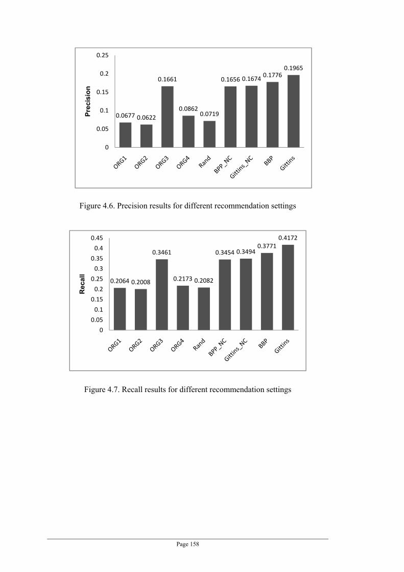
Page 158
Figure 4.6. Precision results for different recommendation settings
Figure 4.7. Recall results for different recommendation settings
0.0677 0.0622
0.1661
0.0862 0.0719
0.1656 0.1674 0.1776
0.1965
0
0.05
0.1
0.15
0.2
0.25
Pre
cisi
on
0.2064 0.2008
0.3461
0.2173 0.2082
0.3454 0.3494 0.3771
0.4172
0
0.05
0.1
0.15
0.2
0.25
0.3
0.35
0.4
0.45
Rec
all

Page 159
Figure 4.8. F1 results for different recommendation settings
4.6 CHAPTER SUMMARY
In this chapter, we suggested a new distributed system paradigm for
recommenders, namely, Ecommerce-oriented Distributed Recommender System
(EDRS). EDRS is designed to allow the recommenders from different organisations or
parties to share recommendations with each other, so all of them can achieve better
recommendation quality and services to their users. In addition, as the recommenders
within the proposed EDRS no longer make recommendations solely on their own efforts,
they are therefore more resistant to the cold-start problems.
In order to facilitate the interaction among the recommenders in the EDRS, a
novel peer profiling and selection strategy is proposed in this chapter. The proposed
strategy profiles and selects recommender peers based on their past recommendation
performance, stability and selection frequency in cluster level, and our experiment
results show that the proposed strategy allows recommender peers to effectively learn
from each other and select the most appropriate peers to provide satisfactory
recommendations to their users.
0.0960 0.0908
0.2089
0.1180 0.1015
0.2084 0.2107 0.2258
0.2499
0
0.05
0.1
0.15
0.2
0.25
0.3
F1

Page 160
Chapter 5
5Conclusions
In the last decade, many techniques have been proposed for improving
recommenders’ recommendation quality and their resistance to the cold-start problem.
Most of these existing techniques focus on exploring new ways to better utilise the
available data and information resources in order to generate better recommendations.
However, given very limited data and information resources, the amount of
improvements that can be achieved by these techniques are also limited. In this thesis, a
novel perspective is proposed for improving the recommendation quality and alleviating
the cold-start problem: enriching the available information resources for the
recommenders. Two novel strategies are presented in this thesis to achieve the
information resource enrichment. The first strategy is to consider other facets of the data
and information resources. Specifically, a novel taxonomy-based recommender system,
HTR, is developed in this research. It is able to mine personal-related user taxonomic
preference information from non-personal related product taxonomic descriptors, and it
then combines this new information resource (user taxonomic preferences) with the
available user rating data to generate recommendations (see Chapter 3). The second
strategy for the information resource enrichment is by gathering information resources
from other parties. An Ecommerce-oriented Distributed Recommender System (EDRS)
is presented in this thesis that allows information resources and recommendations to be
shared by multiple recommenders, and they are then able to utilise the shared
recommendations and resources to generate better recommendations (see Chapter 4).
The techniques presented in this thesis are evaluated with popular experimental datasets

Page 161
(Book Crossing Dataset (http://www.informatik.uni-freiburg.de/~cziegler/BX/)) and
standard recommender framework (Tastes (http://taste.sourceforge.net/)) to ensure the
soundness of the experimental results. The results show that the proposed HTR and
EDRS are able to produce high quality recommendations even in the case of the cold-
start situations.
Section 5.1 presents the main contributions of this research. Section 5.2 discusses
the possible directions for the future work in the area of this research.
5.1 CONTRIBUTIONS
The contributions made by this research are listed below:
Discovering the item preference to item taxonomic preference relation:
In this thesis, the implicit relationship between users’ item preferences and
item taxonomic preferences is investigated. This relationship states that
users share similar item preferences might also share similar item taxonomic
preferences. A novel technique is proposed to efficiently and effectively
mine and extract this relation/knowledge from the combination of user
rating data and product taxonomic descriptors. Additionally, the soundness
of the relationship between user item preference and item taxonomic
preference is also empirically evaluated. The details can be found in Section
3.2.3 and Section 3.3.2.
A novel taxonomy-based recommender system: Based on the proposed
relationship between item preference and item taxonomic preference, a
novel recommender system, HTR, is proposed. HTR is very competitive in
terms of computation efficiency and recommendation quality, and most
importantly, it is able to produce high quality recommendations under

Page 162
severe cold-start situations. The details of HTR and related studies can be
found in Section 3.2 and Section 3.3.3.
A novel distributed recommender system: This thesis suggested that one
of the possible ways to achieve the information enrichment is to obtain
resources from other parties. This research proposed a novel distributed
recommender system namely, EDRS, and it allows recommenders from
different parties to share their recommendation and information resources
with each other to enhance their recommendation quality. The background
rationale, interaction protocol, system infrastructure and design aspects of
the proposed EDRS are comprehensively reviewed and presented in this
thesis. The details can be found in Section 4.2.
A novel recommender peer profiling and selection strategy: In order to
enhance the overall performance of the EDRS, a novel peer profiling and
selection strategy is proposed in this thesis. The proposed strategy profiles
and selects recommender peers based on their average performance,
performance stability and selection frequency, and it allows recommenders
to efficiently learn about each other and choose the most effective peers to
assist in making recommendations. It is shown in the experiments presented
in this thesis, by adopting the proposed profiling and selection strategy the
performance of the EDRS is effectively improved. The related information
and experiments can be found in Section 4.3 and Section 4.5.
Three novel neighbourhood formation related techniques: In addition to
the main contributions of this thesis (i.e. HTR and EDRS), three new
recommender-related techniques are also developed during the research, and
they are:

Page 163
o A novel similarity measure – Statistical Attribute Distance (SAD). It
allows user profile similarity to be more objectively measured by
considering the popularity differences among the attribute values in the
user profiles. The detailed information for SAD is described in Appendix
A.
o A novel clustering algorithm – Hybrid Partitional Clustering (HPC). It
features in its efficiency, accuracy and the ability to produce
automatically optimal cluster partition without involving complicated
manual configurations. The detailed information for HPC is described in
Appendix B.
o A novel neighbourhood estimation technique – Relative Distance
Filtering, (RDF). RDF features in its competitive computation efficiency
and low memory requirement. The detailed information for RDF is
described in Appendix C.
5.2 FUTURE WORK
The concept of information enrichment for recommender systems proposed in
this thesis is general, and there can be many other possible ways to achieve it besides the
two strategies (i.e. HTR and EDRS) presented here. Therefore, it is one of the future
studies to investigate other new strategies to achieve the information enrichment for
recommender systems.
The HTR system presented in this thesis is specifically designed for tree structure
based item taxonomy. Indeed, such taxonomy structure has been widely used by many
ecommerce sites and applications for representing and describing item contents.
However, there are still many other item representation techniques available, and some

Page 164
of them are achieving vast popularity nowadays (e.g. item tags). Hence, it would be a
promising future work to improve the proposed HTR so it can accommodate other item
taxonomy structures or presentations.
The focus of the EDRS in this thesis is on constructing the overall framework
concept, interaction protocol and peer learning strategies. Hence, many detailed aspects
and related techniques are not covered in this thesis. In the future, the proposed EDRS
can be further improved by considering the following works:
While a novel peer profiling and selection technique is presented in this
thesis to allow manager peers to learn about contractor peers, it is desirable
to have learning strategies for contractor peers to learn about the manager
peers. By allowing manager peers and contractor peers to learn from each
other (currently only manager peers are able to profile contractor peers), the
cooperation among the recommender peers can become more effective, and
the performance of the recommender peers can be further improved.
The recommendation merging technique presented in this thesis is rather
trivial, and it can be improved or replaced by more advanced techniques.

Page 165
Appendix A: Statistical Attribute Distance
As described in Section 2.1.2, the basic idea behinds the collaborative filtering
technique is to predict the target user’s item preferences based on the tastes of other
similar minded users. Hence, it can be easily observed that determining similar minded
users for a given target user is one of the most essential parts of the collaborative filtering
based recommenders. Generally, cosine similarity and Euclidean distance are considered
as the two most popularly used similarity measures to determine the degree of similarity
between two user profiles. Assuming that the user profiles are the users’ item
preferences (i.e. item ratings), the following equations are used to calculate the similarity
between two users:
For the cosine similarity measure:
,∑ , ,
∑ , ∑ ,
(A.1)
For the Euclidean distance measure:
, , ,
(A.2)
In both equation (A.1) and (A.2), , are the two users, , 0,1
denotes ’s explicit rating value to item . Moreover, is the set of items

Page 166
that have been explicitly rated by . For more details about the notation, please refer to
Section 3.2.1. Even though the Euclidean distance and cosine similarity measure are
simple and intuitive, they can still be improved in many aspects to better measure user
similarities. For example, the Pearson correlation coefficient measure (see Equation (3.1)
and Section 3.2.2) is often considered as a better alternative than both of these two
methods as it is able to accommodate the differences among users’ rating habits (Breese
et al., 1998, Herlocker et al., 2002, Montaner et al., 2003).
The Inverse User Frequency (IUF) method proposed by Breese (Breese et al.,
1998) was reported to even out perform the Pearson correlation coefficient measure. The
basic rational behinds IUF is to reduce the weights on universally preferred items when
calculating the user preferences to items, because these items are generally considered
less capable of capturing user similarities than uncommon items (Breese et al., 1998).
The proposed Statistic Attribute Distance (SAD) takes the concept of IUF further
by distinguishing the unpopular rating values from the popular rating values. Specifically,
while IUF considers the popularity of each item, the proposed SAD method suggests that
the popularity of each individual rating values rather than each individual item is a better
factor to be considered in similarity computation. The major limitation of IUF is that it is
strongly dependent to the completeness of the dataset and the way the dataset is
constructed (i.e. if the dataset is constructed based on sampling, we need to ensure that
the popularity distribution of the items in the sampled dataset is similar to the original
dataset). In contrast, the popularity of the item ratings in the dataset is less sensitive to
the completeness of the dataset and it allows the proposed SAD to perform a more stable
manner than the IUF.
A.1. MEMORY-BASED COLLABORATIVE FILTERING

Page 167
Memory-based collaborative filtering is the most common type of collaborative
filtering, and it is very intuitive and simple to implement (Breese et al., 1998). In this
section, the existing and proposed similarity measures will be discussed and investigated
in the context of the memory-based collaborative filtering. A typical form of the
memory-based collaborative filtering technique is listed below:
, ,\
,
(A.3)
In Equation (A.3), denotes all users in the dataset who have previously
rated item , and , represents the predicted rating of the target user to
item . and are the average item ratings of the users and respectively. ,
denotes the actual past rating gave to . , is the user similarity measure for
computing the preference similarity between and . Finally, is a normalising
factor such that the values of the weights sum to unity. Based on the equation depicted
above, it can be observed that the accuracy of the predication is strongly dependant on
the computation of the user similarity , between the target user and all other
users who has previously rated . There are many existing techniques can be
employed as the user similarity measure , , some of these techniques are described
previously such as cosine similarity (Equation (A.1)), Euclidean distance (Equation
(A.2)) and Pearson correlation coefficient (Equation (3.1)). Despite the many possible
implementations of , , they all have identical underlying concept: generating a high
value when and have very similar preferences, and a low value if they have no

Page 168
common tastes. In such way, the predicted rating , will approach the actual ratings to
given by the similar minded neighbours of .
A.2. INVERSE USER FREQUENCY
As mentioned earlier, there are still some advanced similarity measures other
than the standard ones such as cosine similarity, Pearson correlation coefficient, etc., and
many of these advanced similarity measures are reported to have better performances
than the standard ones (Breese et al., 1998, Herlocker et al., 2002, Montaner et al., 2003).
Inverse User Frequency (IUF) proposed by Breese et al. (1998) is one of the most known
advanced similarity measures. In this part of work, IUF is employed as the major
benchmark and the comparison work to the proposed SAD method, because it has been
suggested to outperform many other existing similarity measures and also shares certain
concept similarity to the proposed SAD technique. The concept of IUF is briefly
described in this section.
It can be observed from Equation (A.1) and (A.2), the standard similarity
measures consider the all items equally. However, they might be further improved if the
more influenced items can be treated more importantly. The concept behinds IUF came
from the well-known information retrieval technique - Inverse Document Frequency
(IDF) (Salton, 1983) – which is commonly employed to mine the keywords from given
documents. In IDF, a word is considered less important if it occurs commonly among all
the documents. By taking this idea into the collaborative filtering, IUF suggests that the
universally rated items are less useful in capturing the user similarities than uncommon
items. For an item , the following equation can be used to measure the importance of
the item:

Page 169
| || |
where | | is the total number of users in the dataset and | | is the number of users who
have rated for item in the past. With the importance factor defined, the correlation
coefficient method can be modified by using as a weight to represent different
importance for different items. Thus, the IUF is defined as below:
,∑ , ,
∑ , ∑ ,
(A.4)
It can be easily observed that Equation (A.4) is a modification to the standard
Pearson correlation coefficient. Importantly, when comparing the items commonly rated
by and , the two users’ rating similarities towards popularly rated items are
considered insignificant (i.e. is small), in contrast, if the two users have rated
unpopular items similarly (i.e. is large), the two users will be considered as having
strong similar item preference. Therefore, is a very important factor that affects the
final results of IUF. If can be accurately computed (such that it accurately reflects the
item popularities in the entire dataset), then the logic behind IUF is indeed more
objective and appropriated than the standard similarity measures, and therefore can
greatly improve the recommenders’ recommendation quality.
A.3. PROPOSED APPROACH - SAD
In this section, the proposed Statistical Attributed Distance (SAD) method is
explained. The basic idea behinds SAD is to include the influences of attribute values

Page 170
into object correlation measurement. In essence, when comparing an attribute of two
objects, if they have the same value to in the same attribute and the value has a high
population (i.e. many objects have this value for this attribute) in the entire database,
then the similarity in terms of this attribute is considered less important. By contrary, if
the two objects have similar values to the same attribute and the value has a low
population, then the similarity in terms of this attribute is considered important. In the
case of recommender systems with user ratings as user profiles, an object is a user
represented as a vector of item ratings, each item is an attribute and the rating is the value
of the attribute. The user who have the same rating (or very similar rating) to an item and
the rating value is popularly voted to the item by many users, the likeness of the two
users’ rating to this item will not contribute much to determine the similarity between the
two users. For example, suppose that most users have voted an item with rating 7
(i.e. 7 is a popular value to this item), if two users voted this item with rating 3 which is
not popularly voted to this item by other users, the two users are considered more similar
than if they voted this item with rating 7. The concept can be further explained using
Figure A.1 and Figure A.2.
In both Figure A.1 and Figure A.2, axes x and y represent user ratings for two
items, in particular, axis x represents ratings to item and axis y represents ratings to
item . Each dot in the graph represents a user’s ratings to both items. For simplicity,
we only show the positive region (e.g. rating 4-7) and negative region (e.g., rating 1-3)
on each axis to indicate users’ preference to the items. For example, since is placed at
the middle between the positive and negative regions of both items, it indicates ’s
preferences to both of the two items are neutral. Group and are two different
sets of users grouped according to the observable similarity. The users in all rate
positively but negatively to , by contrast, the users in prefer to .
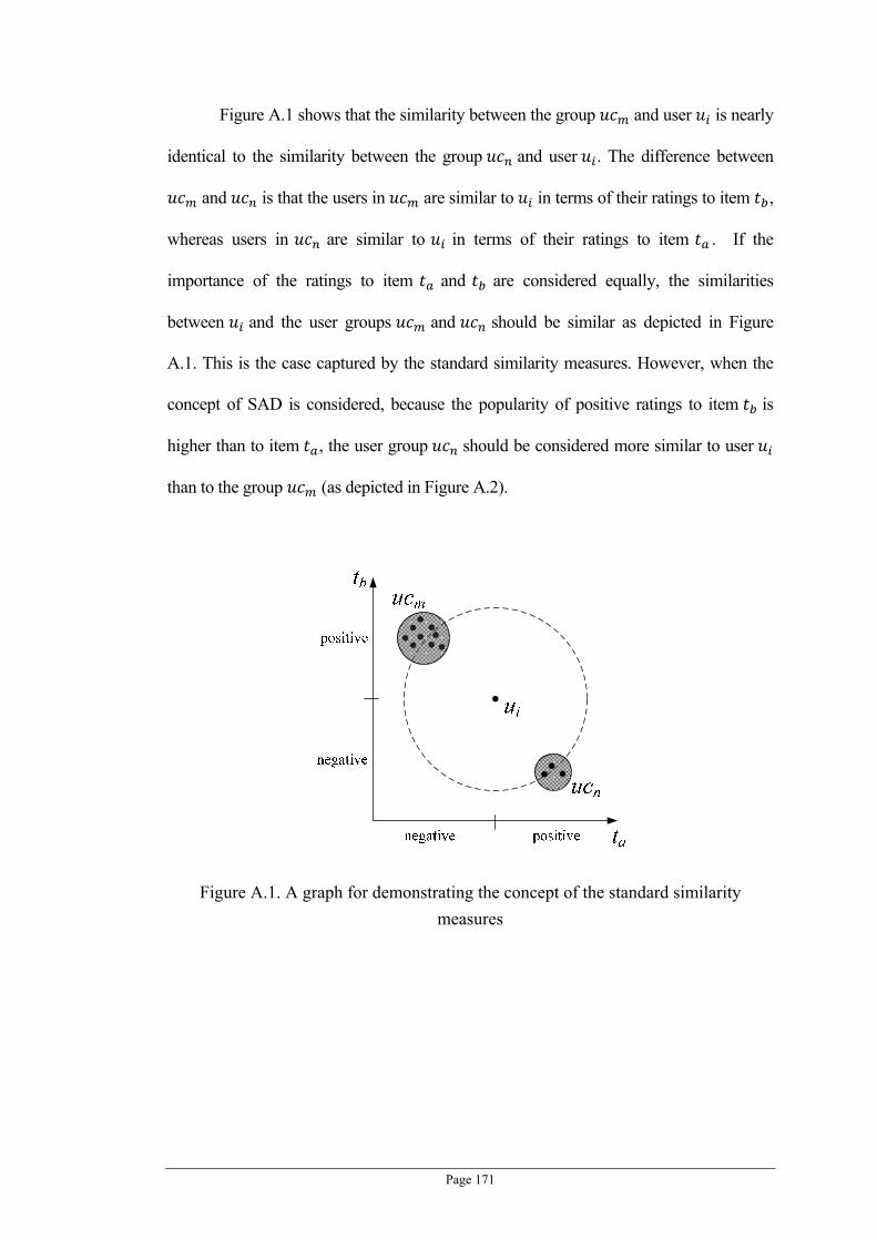
Page 171
Figure A.1 shows that the similarity between the group and user is nearly
identical to the similarity between the group and user . The difference between
and is that the users in are similar to in terms of their ratings to item ,
whereas users in are similar to in terms of their ratings to item . If the
importance of the ratings to item and are considered equally, the similarities
between and the user groups and should be similar as depicted in Figure
A.1. This is the case captured by the standard similarity measures. However, when the
concept of SAD is considered, because the popularity of positive ratings to item is
higher than to item , the user group should be considered more similar to user
than to the group (as depicted in Figure A.2).
Figure A.1. A graph for demonstrating the concept of the standard similarity
measures

Page 172
Figure A.2. A graph for demonstrating the concept of the proposed SAD technique
Based on the concept described above, similar to the factor in the IUF we
define a weight factor as below:
1| || |
where indicates the degree of the uniqueness that a particular rating value is
given to item . In the equation, | | is the total number of users who have previously
rated and | | is the number of users who rated item with a particular value .
It can be easily observed from the equation that when there are many users who rated
item with a particular , the value will be small, conversely, if only a few users
rated with a rating value , will be large. Based on the proposed weight factor
, the proposed SAD method can be formularized as below:
,∑ sv , ,
| |
(A.5)
where

Page 173
sv , ,
, , 1 , 0 , 0
, , 1 , 0 , 0
, ,
and
, ,
In Equation (A.5), sv , , denotes the weighted similarity for and ’s
ratings to item , | | is the number of items rated by both and , and the
constant 0,1 is used to adjust the importance or influence of the weight factor
in sv , , . Specifically, when equals to 0, , acts similar to
standard similarity measures, conversely, when approaches 1, users with similarity in
their uncommon tastes will be considered more important. Moreover, , is a normalised
rating based on , , which is simply the difference between ’s actual rating to and
’s average rating (i.e. ). The idea behind the normalised rating , is adopted from
Pearson correlation coefficient, the main purpose is to reduce the differences among
different users’ personal rating styles. The value of , can be either positive or negative,
when , is positive, it indicates that ’s preference to is above average, conversely,
when , is negative, ’s preference to is below average.
In order to compute the weight factor in Equation (A.5), we firstly need to
enumerate all the possible values for (in such case, needs to be a discrete variable, or
needs to be discretized first), so that we can compute the occurrences of a particular
rating value to a given item . The equation we depicted above took the simplest
approach by discretizing the user ratings into binary variables so that each rating can be
categorized into either “like” (i.e. ) or “dislike” (i.e. ). The normalised rating (i.e. , )
effectively facilitates the desired discretization process; when , 0, it indicates that

Page 174
“likes” (i.e. ), and when , 0, “dislikes” (i.e. ). Hereby, we can then
divide the set of users who previously rated (i.e. ) into two sets and ,
and they denote the set of users who like and dislike respectively. Based on the
divided user sets and , we can then compute the weight factors and
given in Equation (A.5), such that when there are many users who like (i.e.
), will be small and is large; when there are many users
who dislike (i.e. ), will be large and is small.
The use of the weight factors and in sv , , basically
follows the concept of proposed SAD described in the beginning of this section.
Specifically, when both and rated positively (i.e. , 0 and , 0 ) or
negatively (i.e. , 0 and , 0), we include the influences of rating popularity (i.e.
the weight factors and respectively) in the final score. For example, when
two users and both rated item and positively, where is a popular liked
item and is a popularly disliked item, the similarity between and ’s preferences
to will be emphasised over the preference similarity to under the concept of SAD.
That is, the value of sv , , will be larger than the value of sv , , due to
the weight factors .
In the third case of sv , , where and have completely different
preferences about (e.g. , 0 and , 0), sv , , will return a negative
value (since , , will be negative), and the weight factor will not be included in
the computation (i.e. we don’t need to emphasise on the differences between two users’
ratings to an item).
To summarise, Equation (A.5) has precisely implemented the concept of the
proposed SAD described in the beginning of this section. Note, while Equation (A.5)

Page 175
only discretizes the rating values into “like” and “dislike” (i.e. binary discretization) for
the simplicity, one can always extend the SAD concept further with more advanced
discretization methods (e.g. discretize the rating values into five levels such as “hate”,
“dislike”, “neutral”, “like”, “love”) to obtain better results.
A.4. EXPERIMENT AND EVALUATION
In this section, the experimental results we obtained from comparing the
predictive accuracy between IUF and the proposed SAD method are presented.
A.4.1. Data Acquisition
The dataset used in this experiment is obtained from MovieLens project
(http://www.movielens.org/), and it was collected through the MovieLens web site
during the seven-month period from 1997 to 1998. The dataset is cleaned up so each
user has at least 20 ratings (i.e. | | 20). The dataset contains 100,000 ratings from
900 users on 1682 movies.
From these 900 users in the dataset, 100 of them are randomly selected into the
testing user set and the rest of 800 users are then used to form the training user set. In the
testing user set, each testing user ’s ratings are divided into two parts: the training
ratings and the testing ratings , such that and . The testing
rating set contains 10 ratings that are randomly selected from (i.e. | | 10), and
the rest of the ratings are used to form the testing user ratings .
A.4.2. Evaluation Metrics

Page 176
The prediction quality of IUF and SAD is evaluated by the Mean Absolute Error
(MAE) metrics (Breese et al., 1998, Zeng et al., 2003), and it is depicted as below:
MAE∑ | , , |
| |
(A.6)
In Equation (A.6), denotes a item involved in ’s testing rating list , and
, and , each denotes the predicted rating and actual rating that gives to
respectively.
In this experiment, the 800 users in the training user set are used to train the
prediction algorithms IUF and SAD. We then cycle through each of the 100 user in the
testing user set, and treat each of them as a target user for the prediction algorithms.
Specifically, with a given target user , Equation (A.6) is applied to compute the
prediction algorithms’ (i.e. IUF and SAD) average miss-predictions to . Then we sum
up the results for every in the testing user set, and compute the average in order to
obtain the average miss-predictions (i.e. MAE) for IUF and SAD.
A.4.3. Experimental Results
In the section, the experimental results obtained from evaluating the IUF and
SAD methods with the MAE metrics are presented. The experiment was conducted
based on training user sets of different sizes ranging from 100 to 800.
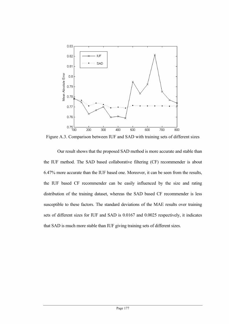
Page 177
Figure A.3. Comparison between IUF and SAD with training sets of different sizes
Our result shows that the proposed SAD method is more accurate and stable than
the IUF method. The SAD based collaborative filtering (CF) recommender is about
6.47% more accurate than the IUF based one. Moreover, it can be seen from the results,
the IUF based CF recommender can be easily influenced by the size and rating
distribution of the training dataset, whereas the SAD based CF recommender is less
susceptible to these factors. The standard deviations of the MAE results over training
sets of different sizes for IUF and SAD is 0.0167 and 0.0025 respectively, it indicates
that SAD is much more stable than IUF giving training sets of different sizes.
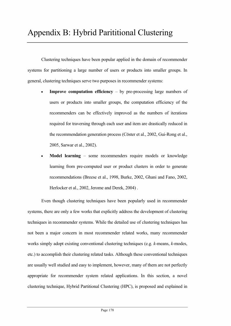
Page 178
Appendix B: Hybrid Parititional Clustering
Clustering techniques have been popular applied in the domain of recommender
systems for partitioning a large number of users or products into smaller groups. In
general, clustering techniques serve two purposes in recommender systems:
Improve computation efficiency – by pre-processing large numbers of
users or products into smaller groups, the computation efficiency of the
recommenders can be effectively improved as the numbers of iterations
required for traversing through each user and item are drastically reduced in
the recommendation generation process (Cöster et al., 2002, Gui-Rong et al.,
2005, Sarwar et al., 2002).
Model learning – some recommenders require models or knowledge
learning from pre-computed user or product clusters in order to generate
recommendations (Breese et al., 1998, Burke, 2002, Ghani and Fano, 2002,
Herlocker et al., 2002, Jerome and Derek, 2004) .
Even though clustering techniques have been popularly used in recommender
systems, there are only a few works that explicitly address the development of clustering
techniques in recommender systems. While the detailed use of clustering techniques has
not been a major concern in most recommender related works, many recommender
works simply adopt existing conventional clustering techniques (e.g. k-means, k-modes,
etc.) to accomplish their clustering related tasks. Although these conventional techniques
are usually well studied and easy to implement, however, many of them are not perfectly
appropriate for recommender system related applications. In this section, a novel
clustering technique, Hybrid Partitional Clustering (HPC), is proposed and explained in
Page 179
detail. The proposed HPC technique can automatically estimates the optimal number of
clusters for a given dataset, and so it can be easily adopted by recommenders as they
don’t need to manually estimate the appropriate numbers of clusters to achieve optimal
performances in their recommendation making processes. Moreover, the proposed HPC
technique allows the resulting cluster partitions to gradually update themselves when
there are updates to the datasets, and it ensures the cluster partitions are always
consistent with the underlying datasets so that the hosting recommenders are always in
the optimal states. Before the proposed HPC technique is explained, some existing and
state-of-the-art clustering techniques are briefly reviewed in Section B.1.
B.1. EXISTING CLUSTERING TECHNIQUES
Clustering is an unsupervised classification process that partitions a large set of
data or objects (or users and items in the context of recommender systems) into
homogeneous clusters. As the ‘unsupervised nature’ indicated, it is often assumed that
the clustering users have minimal information and knowledge to the data being observed.
Therefore, the major objective of clustering is to organise the mass and disorderly
objects into a set of meaningful clusters (Jain et al., 1999). Clustering plays an
outstanding role in several research fields such as scientific data exploration, information
retrieval and text mining, spatial database applications, Web analysis, customer
relationship management (CRM), marketing, medical diagnostics, computational
biology, and many others (Berkhin, 2002), therefore huge amounts of works have been
done in this area. Detailed reviews and surveys about the current state-of-the-art
clustering techniques can be found in (Berkhin, 2002, Jain et al., 1999, Pedrycz, 2005).
Clustering techniques can be broadly divided into two categories, namely,
partitional clustering and hierarchical clustering. For partitional clustering techniques,

Page 180
various partitions containing clusters are constructed, and based on some criterion the
partition that minimises (or maximises) a predefined objective function is then chosen
(Frigui and Krishnapuram, 1997, Pedrycz, 2005). However, a major shortcoming of the
partitional clustering is that the number of resulting clusters (i.e. ) has to be specified in
advance, and it is difficult for users to supply the exact value of manually when their
knowledge to the data is limited. Moreover, some partitional clustering techniques such
as k-means and k-modes are prone to local optimum and their clustering results are
sensitive to initial locations of the cluster centres (i.e. these techniques often randomly
select points in the initialisation stage, and iteratively adjust them to the correct cluster
centre locations to form clusters). Conversely, hierarchical clustering techniques create a
hierarchical decomposition of dataset and it is often represented in a form of dendrogram.
A partition in hierarchical clustering can be obtained by cutting the dendrogram at some
desired level, and therefore it is not required to specify the number of output clusters in
advance. Notwithstanding hierarchical clustering provides better analytic features than
partitional clustering (as data can be visualised in a dendrogram), it generally does not
scale well for large datasets. In addition, in classical hierarchical clustering (e.g.
agglomerative and divisive based hierarchical clustering) objects that are committed to a
cluster in the early stages cannot move to another cluster. In other words, once a cluster
is split or two clusters are merged, the split objects will never come together in one
cluster or the merged objects will always stay in the same cluster, no matter whether the
splitting or the merge is a right action or not. It is shown in (Pelleg and Moore, 2000, Xu,
2005), some previous splitting or merging actions in hierarchical clustering maybe not
right and some split and merged objects may need to be rearranged in latter actions. This
particular issue is the major cause of inaccuracy in hierarchical clustering, especially for
large datasets.

Page 181
Besides these two classical techniques, there are also some extensions and
advanced clustering techniques designed to address the limitations of the classical
clustering techniques. The X-means suggested by Pelleg and Moore (2000) is one of the
most popular extensions to classical k-means. X-means saves users from specify the
exact (i.e. number of resulting clusters); instead, users only need to specify a possible
range of , and the X-means will return the optimal partition within the specified range.
Likas et al. (2003) tries to produce the optimal partition by using an incremental
technique that dynamically add one cluster centre at a time through a deterministic
global search procedure from suitable initial positions. Pelleg and Moore (1999) utilise
the kd-tree data structure and the geometric reasoning techniques to estimate the initial
locations of the cluster centroids. In contrast to Pelleg and Moore (1999)’s work, Al-
Daoud (2005) proposed a less sophisticated centroid initialisation method based on
finding a set of medians extracted from a data dimension with maximum variance.
The proposed HPC technique addresses not only the limitations of both the
standard partitional and hierarchical clustering techniques, but it also provides some
advantages over other advanced clustering techniques. A general overview of HPC’s
algorithmic concept and some comparisons between HPC and the existing clustering
techniques described above are provided in Section B.2.
B.2. GENERAL OVERVIEW
The proposed HPC technique consists of three consecutive phases: initial
centroids estimation, partitional clustering and hybrid partition adjustment and
optimisation (as depicted in Figure B.1). In the first phase, for a given dataset the most
possible number of clusters and the possible centroids of the potential clusters are
estimated with a novel centroid estimation technique. In the second phase, the estimated

Page 182
centroids are utilised to initialise a standard partitional clustering technique (e.g. k-
means), and then the initial cluster partition can be obtained by executing the selected
partitional clustering technique. In the final phase, a incremental clustering algorithm,
Hybrid Hierarchical Clustering Algorithm (HHCA), proposed by (Xu, 2005) is
employed to further optimise the initial cluster partition resulted from the second phase
based on a predefined objective function.
Figure B.1. The three major consecutive phases of the proposed HPC technique
One of the advantages provided by the HPC technique is that neither the number
nor the range of the possible clusters needs to be specified in advance. Therefore, the
HPC technique provides better usability than standard partitional clustering techniques

Page 183
such as k-means, k-modes, etc. or even more advanced techniques like X-means, which
require the range of resulting clusters to be pre-specified.
Partitional based clustering techniques such as k-means and k-modes usually
provide only local optimal clustering solutions. It is mainly because their clustering
results are strongly dependent on the initial centroids selections which are often based on
randomisation (Jain et al., 1999). Hence, when conducting multiple trials in one dataset,
partitional based techniques (e.g. k-means and k-modes) usually produce clustering
results with different quality. Specifically, when they are initialised with centroids that
are closer to the true centroids locations, the efficiency and the resulted clustering
qualities can be greatly improved, conversely, poor chosen centroids for the initialisation
might result in poor performance and clustering results. Standard techniques based on
randomised centroids initialisation (i.e. k-means, k-modes etc.) usually need to be
executed in numerous runs (with different centroids initialisations) in order to determine
which clustering results are closer to the optimal solution. Obviously, such solution is
impractical, inefficient and error-prone when the target dataset is large. As mentioned
before, some existing centroids location estimation techniques have been proposed to
improve the performance of the partitional based techniques (e.g. (Al-Daoud, 2005,
Pelleg and Moore, 1999)) , and they all reported to have achieved certain amount of
improvements over standard techniques in their experiments. However, to the best of
our knowledge, none of them can both automatically estimate the number of centroids
and their corresponding locations for the given dataset, and many of them can only
estimate the centroid locations with the number of centroids been manually specified in
advance. In contrast, the proposed centroids estimation technique used in the first phase
of the HPC can estimate both the number of centroids and their locations for any given
datasets. Hence it not only provided a better usability than other techniques but also

Page 184
enables the partitional clustering technique used in the second phase to perform more
efficiently and result better quality for the initial clustering partition.
In the final phase of HPC, the initial clustering partition resulted from the second
phase is further optimised in accordance to a predefined objective function (see Section
B.3). The purpose of the objective function is to allow users to specify the desired cluster
granularity while not interfere the overall clustering quality. Specifically, depending on
different usages, users can specify if they need the clustering results to have a large
numbers of clusters with higher densities in each of the clusters or a smaller numbers of
clusters and each with lower densities. This design provides better usability than both
partitional and hierarchical based techniques, because it enables the users a certain
flexibility to control their desired clustering results and allows them to have minimal
knowledge to the target datasets (i.e. do not need to know the size or the density of the
dataset). In order to optimise the initial clustering partition from the second phase, the
employed HHCA iteratively merges and splits the clusters in the partition until the
objective function is maximised. In particular, unlike standard hierarchical clustering
techniques where clusters can only be merged or split but not both, HHCA allows
clusters to be split or merged in every partition updates. Hence given two objects that
have been divided into two different clusters, they might be merged into one cluster in
latter update iterations. This feature allows HHCA to produce better clustering results
than other hierarchical based techniques and also be able to cope with frequent dataset
updates (i.e. when the objects are added, removed or modified in the datasets, the
corresponding clustering partitions can be efficiently adjusted based on the changes).
The details of the HPC and the three phases are to be detailed in the following
sections. In Section B.3, the objective function we employed to evaluate the quality of

Page 185
resulting partition is summarised. Section B.4, B.5 and B.6 explain the three consecutive
phases of the proposed HPC technique respectively.
B.3. OBJECTIVE FUNCTION
As in the notion of the partitional clustering, a clustering problem can be
considered as an optimisation problem to a predetermined objective function. In this
work, the objective function defined in (Xu, 2005) is employed. By solving the
maximum of objective function, the resulting partition will have maximum intra-cluster
similarity and maximum inter-cluster distance. In other words, it is expected that the
objects within a cluster are as close as possible and the objects in different clusters are as
far as possible.
Let , , … , be a set of given data objects, where each data point
can be represented as a p-dimensional vector in a vector space. For a given , we
assume , , … , be a partition over the dataset where for all
and . Moreover, the cluster centroid (i.e. cluster median or central
id) for is denoted as , , , , … , , , where , indicates the dimension
of ’s cluster centroid. Note, because HPC is a very general technique and can be
applied to many different applications (not just for recommender systems), therefore, we
will use some new notations in this section that are less specific to recommender systems
(i.e. different notations from those employed in previous chapters). For example, an
object can be either a user or an item in recommender systems depending on the target
recommender types (e.g. collaborative filtering vs. item-to-item collaborative filtering).
However, for the understandability, readers can assume that each object
corresponds to a user in a recommender system, the object attributes are the user

Page 186
ratings, and the goal is to divide the entire user set into user clusters (i.e.
corresponds to ).
Before defining the cluster intra-similarity and inter-distance, it is important to
specify how the similarity and distance between two objects (or data points) are
measured. In this work the two commonly used measurements, cosine similarity and
Euclidean distance measure, are chosen to measure the similarity of objects:
,
(B.1)
,
(B.2)
where , are two objects.
When and are considered as two users in a recommender system, their
cosine similarity and Euclidean distance can be computed by Equation (B.1) and (B.2)
respectively. Moreover, depending on the target dataset and application, the cosine
similarity and Euclidean distance measures can be replaced with other similarity and
distance measures such as those described in Appendix A.
The intra-similarity of a cluster is simply the average of the similarities
between all the objects within and the cluster centroid . Specifically:
intra_sim∑ ,
| |
(B.3)

Page 187
Based on Equation (B.3) we can then further measure the average cluster intra-
similarity of a given partition (or a clustering result) :
p_intra_sim∑ intra_sim
| |
(B.4)
While cluster intra-similarity measure can be used to determine the cluster
densities (i.e. whether the objects within in a cluster are closed to each other), we also
need to be able to measure the distance between two different clusters (i.e. whether the
objects in different clusters are far way from each other). In this work, the distance
between two clusters is measured by calculating the distance between their centroids:
cluster_dist , dist ,
(B.5)
Based on Equation (B.5), we can then evaluate the overall cluster inter-distances
of a given partition by simply averaging the distances of all the possible cluster pairs
from the partition:
p_inter_dist∑ cluster_dist ,, ,
| | | | 1
(B.6)
Finally, by combining Equations (B.4) and (B.6), the objective function (i.e.
quality of a given partition) is given by:

Page 188
p_qual p_inter_dist 1 p_intra_sim
(B.7)
where 0 1 is used to adjust the weights of the cluster inter-distance and intra-
similarity in the final partition quality scores.
By observing closely the cluster inter-distance and intra-similarity measures
defined in Equations (B.4) and (B.6), it can be seen that they have different reflections
on the partition granularities. Specifically, the cluster intra-similarity measure trends to
give higher scores to partitions with large number of small clusters, because small
clusters usually have higher densities (i.e. cluster intra-similarities) than large clusters. In
contrast, the cluster inter-distance measure trends to give higher scores to partitions with
small number of large clusters, because the centroids of large clusters are usually more
distant from each other than centroids of small clusters. Hence, the control parameter
used in Equation (B.7) can be used to adjust the desired partition granularities. When
is set to values closed to 1, the cluster inter-distance is considered more important than
the cluster intra-similarity, thus, Equation (B.7) will give higher scores to partitions with
small number of large clusters (i.e. partitions with low granularities). Similarly, when
is set to values closed to 0, the cluster intra-similarity will receive higher weight, and
hence Equation (B.7) will give higher scores to partitions with large number of small
clusters (i.e. partitions with high granularities). Thus, by adjusting the control parameter
, users can easily and effectively adjust the desired granularities of the cluster partitions
generated by the proposed HPC technique.
B.4. CLUSTER CENTRE ESTIMATION

Page 189
The proposed cluster centroid estimation technique is intuitive, effective and
considerably efficient, and provides the following three features:
Estimation of the possible number of potential clusters.
Estimation of the centroid locations of the potential clusters.
Outlier detection.
B.4.1. Cluster Centroid
Before going into the details of the proposed centroid estimation technique, it is
important to understand the basic nature of a cluster centroid.
In k-means, a cluster centroid is the average of all the data points in a cluster. In
other words, its coordinates are the arithmetic mean for each dimension separately over
all the points in the cluster. On the other hand, the cluster centroid in k-modes is the
median data point in the cluster. A more descriptive explanation to the concept of cluster
centroid is given in Fuzzy C-Means (FCM) (Berkhin, 2002, Pedrycz, 2005):
,
(B.8)
where is the centroid of cluster and is a membership function measuring the
likelihood that the object belongs to the cluster . The C-means clustering method is
to find cluster which maximise Equation (B.8) . Equation (B.8) indicates the following
features:

Page 190
A cluster centroid is an object (can be either a virtual or actual object or data
point) within a cluster, such that the distances between it and all other
objects in the cluster are averagely shortest.
The distances between the cluster centroid and all other objects outside the
cluster are insignificant (i.e. they were filtered out by given very small
values of ).
B.4.2. Single Cluster Centroid Estimation
For the simplest case where the dataset containing only a single cluster (i.e.
| | 1), we can find the arithmetic mean or median of the objects in the cluster as the
centroid, and it is the commonly used approach in k-means and k-modes. In our case,
however, it is required to find the cluster centroids based on only the distances among
the data points, and there are several reasons for it:
Standard arithmetic mean or median computes only centre locations for
given clusters, however, the computed centroid results do not contain
information about the cluster densities. However, in the proposed centroid
estimation algorithm, it is required to compare centroids of multiple clusters
based on their cluster densities. Hence, standard arithmetic mean or median
for computing cluster centroids does not suit the proposed centroid
estimation algorithm.
Standard arithmetic mean or median is only applicable to objects in standard
vector space. However, they might not be applicable to other complex
objects (e.g. objects with categorical attributes).
Standard arithmetic mean or median might be inconsistent with the
similarity measures employed. As a cluster centre needs to be similarly

Page 191
distant to all of the objects within a cluster, therefore, it should be dependent
on the similarity (or distance) measure employed. However, standard
arithmetic mean or median is independent of the similarity measure
employed. Hence, when advanced similarity measures such as Pearson
correlation coefficient, IUF, SAD, etc. are employed, the centroids
computed by the standard arithmetic mean or median might not be the
desired ones.
In order to find the cluster centroid based on only object distances, we define
as the weight of the object , and specifically:
,\
(B.9)
Then, the possible centroid of (note, we assume there is only one cluster in , so
all objects in is contained in that cluster) can be estimated by:
arg max
(B.10)
is the object that is close to all other objects in the cluster averagely. It can be
observed that Equation (B.9) has a strong connection with Equation (B.8). In Equation
(B.9) it is assumed that all objects in the cluster are possible centroids, and the
membership function in Equation (B.8) is replaced by , .

Page 192
As similar to Equation (B.8), the larger value of indicates the larger
possibility that is the cluster centroids. Hence, the cluster centroids for a single cluster
dataset can be obtained by resolving Equation (B.10). Figure B.2 depicts a possible data
distribution of a single cluster, and the objects with their corresponding weight values
(computed by Equation (B.9)) are depicted in Figure B.3.
Figure B.2. A possible dataset with a single cluster
Figure B.3. An example of centroid estimation based on Equation (B.10)
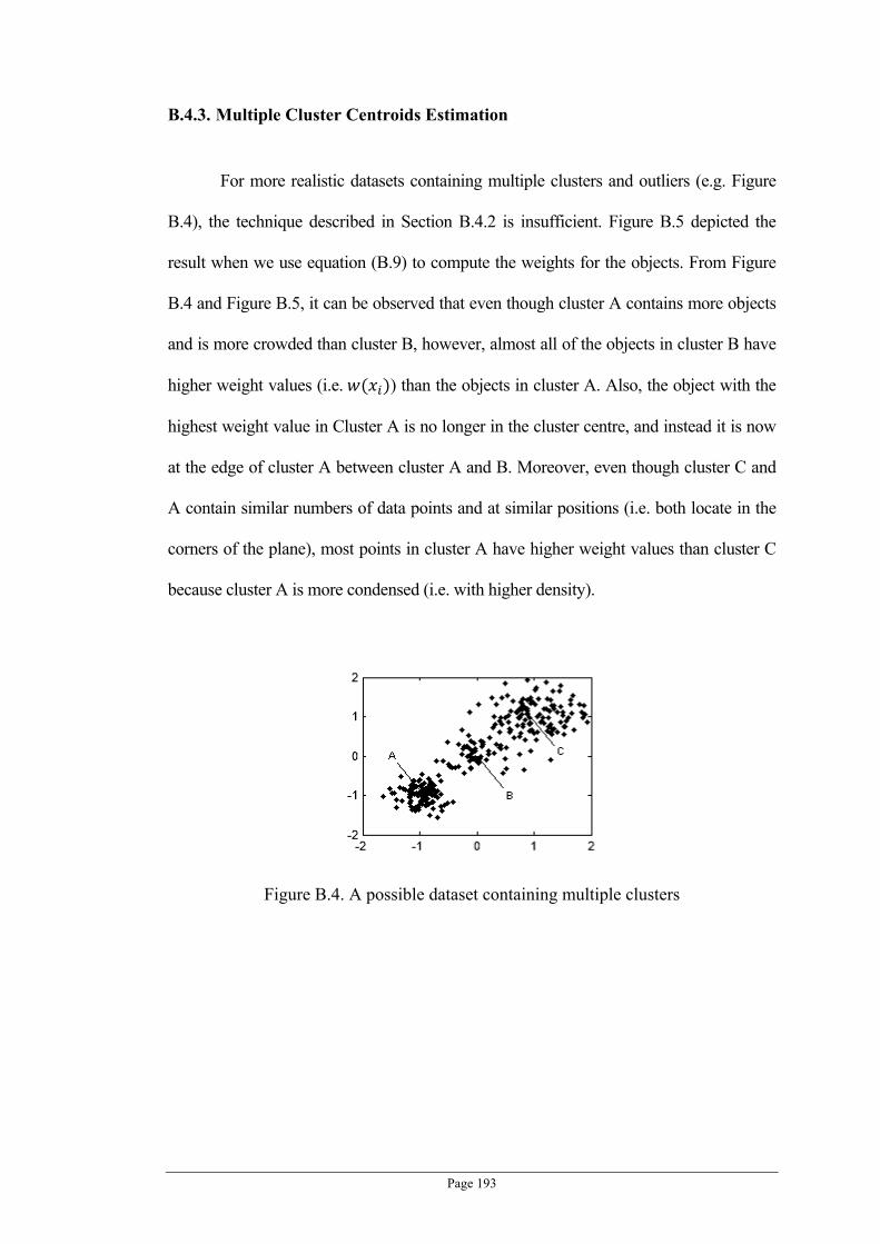
Page 193
B.4.3. Multiple Cluster Centroids Estimation
For more realistic datasets containing multiple clusters and outliers (e.g. Figure
B.4), the technique described in Section B.4.2 is insufficient. Figure B.5 depicted the
result when we use equation (B.9) to compute the weights for the objects. From Figure
B.4 and Figure B.5, it can be observed that even though cluster A contains more objects
and is more crowded than cluster B, however, almost all of the objects in cluster B have
higher weight values (i.e. ) than the objects in cluster A. Also, the object with the
highest weight value in Cluster A is no longer in the cluster centre, and instead it is now
at the edge of cluster A between cluster A and B. Moreover, even though cluster C and
A contain similar numbers of data points and at similar positions (i.e. both locate in the
corners of the plane), most points in cluster A have higher weight values than cluster C
because cluster A is more condensed (i.e. with higher density).
Figure B.4. A possible dataset containing multiple clusters

Page 194
Figure B.5. Centroids estimation for the complex dataset with multiple clusters based
on Equation (B.10)
Figure B.6. An example of virtual boundaries for each of the clusters in the dataset
To summaries, the reasons that why Equation (B.9) failed to produce higher
values for possible cluster centroids of the clusters in the dataset are:
It trends to produce higher weight values for the objects at the centre of the
dataset instead of the centres of the clusters.
Because the size and density are different for different clusters, the weights
of the data points for one cluster are not comparable to other clusters. That is,
the cluster centre of a sparse cluster might have a smaller weight value than
most of the data points in a condensed cluster.
In order to estimate the cluster centroids for dataset consisting of multiple
clusters with different densities, we need to revise the weight computation algorithm so

Page 195
that the weight value of an object won’t be influenced by objects in other clusters. That
is, when computing the weight for an object, we need to estimate a cluster boundary
(such as the circles plotted in Figure B.6) so that any points outside the boundary is
considered inexistent. In this work, we proposed a simple technique using the average
shortest distance of the dataset to estimate the boundary length for the dataset as
described in Equation (B.10):
∑
| |
(B.11)
where is the distance from to its nearest neighbour object, that is:
min,
,
Based on the computed by Equation (B.11) we can then find the
neighbour objects within the boundary of a given object . The set of neighbour
objects of denoted as , is estimated by:
| , ,
only contains the objects that are most likely in the same cluster with .
Therefore, when adopting this boundary constraint to Equation (B.9), the unnecessary
influences from the objects of other clusters are effectively reduced. Specifically,
Equation (B.9) can be modified to:
,,
(B.12)

Page 196
With Equation (B.12) the proposed cluster centroid estimation algorithm, thus,
can be described as below:
Algorithm B.1. _
Input is the object set to which the centroids are to be estimated.
Output is the set of estimated cluster centroids of
1) SET as the set of the estimated centroids and it is initially empty.
2) Find the most possible centroid for the current dataset X based on Equation
(B.12) and Equation (B.10). Specifically:
arg max
3) SET . That is, add the most possible centroid of the current dataset to
.
4) SET \ . Remove the centroid from the dataset.
5) SET \ . Remove all ’s neighbour objects from the dataset.
6) IF | | 0
7) THEN return Z as the set of estimated cluster centroids.
8) ELSE go to step 2.
The idea behinds the proposed method is quite intuitive. Firstly, in line (2) of the
algorithm, the object in the centre of the most crowded object group is considered as the
most possible centroid . Next, the estimated centroid is recorded (i.e. line (3)) and
removed from the dataset (line (4)). Then all neighbour objects of are also removed
from , because they have higher possibility to be in ‘s cluster than to be the centroids
of other clusters (line (5)). The procedure from line (2) to line (7) of the algorithm is

Page 197
repeated until no more possible centroids can be found in (i.e. when becomes
empty).
As example is given in Figure B.7 which illustrates the process of estimating the
cluster centroids using Algorithm B.1. In Figure B.7(a) the centroid in cluster A has the
highest weight than the centroids in cluster B and C as cluster A has the highest density
(i.e. all objects in the cluster are close to each other). After the most possible cluster
centroid has been detected as shown in Figure B.7(a), the detected centroid and its
surrounding neighbours are removed from the dataset in order to allow the centroids of
other clusters to be detected in following rounds. Figure B.7(b) shows the resulting
dataset after the removal of detected centroid and its neighbour objects in Figure B.7(a).
Similarly, Figure B.7(c) shows the resulting dataset after the second most possible
centroid and its neighbour objects are removed from the dataset in Figure B.7(b). It is
worth noting that the last few estimated centroids are very likely to be outliers (see
Figure B.7(d)) , hence the proposed technique can also be used for outlier detection.
Figure B.7. An example of cluster centroids estimation process
B.5. PARTITIONAL CLUSTERING

Page 198
As mentioned earlier, the centroids detected with the centroid estimation
technique described in Section B.4 are not perfectly accurate, they are mainly designed
as the initial centroids for using partitional clustering techniques to complete clustering
tasks. Algorithm B.2 given below is a modified k-means method, which uses the
estimated centroids as the initial centroids of possible clusters.
Algorithm B.2 . _
Input , … , is the set of estimated centroids returned from
Algorithm B.1 (i.e. _ ).
Output is the resulting cluster partition for the dataset
1) SET , … , as the initial partition consisting | | empty clusters,
specifically, : .
2) Associate each cluster with a corresponding centroid from , so that
denotes the centroid of .
3) Assign the objects in to their nearest clusters, such that:
: | , min ,
4) Update the cluster centroids by computing the arithmetic means of the clusters, and
let be the new set of cluster centroids.
5) IF
6) THEN return as the resulted partition.
7) ELSE SET and go to step 3.
By initialising the k-means with the estimated centroids, the possibility of
obtaining local optimal partition results is reduced. In order to demonstrate the

Page 199
effectiveness of the estimated centroids to the k-means method, a simple experiment is
conducted to evaluate the computation efficiency and the clustering quality (calculated
based on Equation (B.7)) by comparing with the following three techniques:
The standard k-means technique with a randomly generated .
The modified k-means method proposed in this section, i.e. initialising the
standard k-means technique with the estimated centroids as described in
Algorithm B.2.
The standard k-means technique with the estimated . That is, instead of
initialising the k-means with the estimated centroids, we only use the
number of the estimated centroids ( ) as the initialisation parameter.
The datasets employed in the experiments are sets of randomly generated two
dimensional vectors with different sizes and densities. The experimental results for
evaluating the clustering quality and computation efficiency are depicted in Figure B.8.
and Figure B.9. respectively. Note, in the computation efficiency experiments (i.e.
Figure B.9. ), the computation efficiency of the standard k-means is not included in the
comparison. It is because the major purpose of the experiments is to test whether the
predicted centroids are relatively accurate so that the iterative centroids refinement
process in the standard k-means can be effectively reduced (and therefore results in
better computation efficiency). The computation efficiency of the standard k-means
(both and centroids are randomly generated) is unnecessary because it is difficult to
determine whether the computation efficiency of the standard k-means comes from the
randomly generated or centroid locations.
It is shown in Figure B.8. that the partition quality (measured based on
Equation (B.7)) achieved by initialising the standard k-means with the estimated is
improved comparing to the standard k-means with a random . This result demonstrated

Page 200
that the number of clusters estimated with the proposed technique is relatively close to
the true number of clusters in a dataset. Moreover, it is also shown in Figure B.8. that by
including both estimated and centroid locations in the k-means, the best clustering
results are achieved, hence it can be further concluded that the centroid location
estimated by the proposed method is accurate as well.
In Figure B.9. , it is shown that by including the estimated centroid locations
into the k-means the computation efficiency can be achieved almost twice as efficient as
the k-means with randomly selected centroids. This improvement suggests that the
estimated initial cluster centroids are close to the correct locations, so that the amount of
time required to find the correct centroids locations is greatly reduced.
To summarise, based on the results obtained from this simple experiment, it can
be concluded that the proposed centroids estimation technique is accurate and its
application to the standard partitional clustering algorithms (i.e. k-means) is beneficial in
both computation efficiency and clustering partition quality.
Figure B.8. Partition quality comparison with different k-means settings

Page 201
Figure B.9. Computation time comparison with different k-means settings
B.6. PARTITION ADJUSTMENT AND OPTIMISATION
In the third phase of the proposed HPC approach, the HHCA method (Xu, 2005)
is employed to fine-tune the clustering partitions so the objective function (B.7) can be
satisfied. The HHCA method is different from the standard hierarchical clustering
methods, it allows the previously committed clusters to be revised in both divisive and
agglomerative manners. With HHCA, a partition is iteratively fine-tuned by comparing
the current partition with new partitions generated by a divisive strategy and an
agglomerative strategy. The detail of HHCA is described below:
Algorithm B.3
Input , … , is the target partition generated from Algorithm B.2 (i.e.
_ ) for the further adjustment and optimisation.
Output is the resulting cluster partition for the dataset
1) SET , … , as the initial partition consisting | | empty clusters,
specifically, : .
2) Customise the objective function (Equation (B.7)) by setting the partition
granularity control parameter (as described in Section B.3).
3) Find a cluster with minimal intra-similarity:

Page 202
argmin intra_sim
4) Find the two most dissimilar objects and in :
, argmax,
dist ,
5) Dividing into and based on and , such that:
| , ,
| , ,
6) Create a new partition by removing from and adding the two clusters
and created in step 5:
\ ,
7) Find the two most similar clusters and in :
, argmin, ,
cluster_dist ,
8) Create a new partition by removing and from and adding in the union
of and :
\ ,
9) Evaluate the qualities of the three partitions , and based on Equation (B.7).
10) IF p_qual p_qual and p_qual p_qual
11) THEN SET and go to step 3.
12) ELSE IF p_qual p_qual and p_qual p_qual
13) THEN SET and go to step 3.
14) ELSE return as the resulted partition.
Because the main function of the HHCA algorithm is to optimise an already
existed partition, it can also be used to update existing cluster partitions. When a cluster
partition is constructed from a dataset, it is possible that the latter updates (i.e. adding,

Page 203
removing and modifying objects) to the dataset might reduce the quality of the cluster
partition. Hence, the proposed HHCA technique can be employed to optimise the
partition after the dataset updates. Since the HHCA technique updates existing partitions
incrementally along with the dataset updates (i.e. do not need to execute the entire
clustering process from scratch), it ensures competitive computation efficiency for the
partition update process.
B.7. EXPERIMENT AND EVALUATION
In this section, the experimental results we obtained from evaluating the
efficiency and effectiveness of the proposed HPC technique are presented.
B.7.1. Data Acquisition
The experiments described in this section were conducted using web server logs
of individual browsing records for users at the msnbc.com site. The server-log files have
been converted into a set of browsing sequences, one sequence for each user session, and
the sequence is represented as an ordered list of category indicators. An example of the
user sequences is given in Table B.1.
Table B.1. An example experimental dataset
User Browsing Sequence
1 FRONT PAGE, NEWS, TRAVEL, TRAVEL
2 NEWS, NEWS, NEWS, NEWS, NEWS
3 FRONT PAGE, NEWS, FRONT PAGE, NEWS

Page 204
4 FRONT PAGE, SPORTS, NEWS, NEWS
5 WEATHER
The clustering task for this dataset is to group these browsing sessions based, so
we can observe and analyse the different types of browsing behaviours. There are
originally 989818 user browsing sequences in the dataset, and each user has visited
around 5.7 pages averagely. In our experiment, we removed from the log files the users
who visited less than 5 pages or more than 10 pages, so the dataset contains only 10000
users after pruning. It might be noticed the user browsing sequences (data points) belong
to categorical data, therefore, Equation (B.1) and (B.2) are no longer suitable for
measuring the similarity or distance of the data points. In the experiment we used the
percent disagreement to measure the distance between two data points:
,∑ ,
where is the vector dimension of the data points, denotes the dimension value of
, and
,0,
1,
B.7.2. Evaluation Metrics
One of the most obvious ways to evaluate the effectiveness of the clustering
techniques is to examine the quality of the resulting cluster partitions. In the experiment,
the partition quality measure depicted in Equation (B.7) is used to evaluate the cluster
partitions produced by the experimental clustering algorithms.

Page 205
B.7.3. Experimental Results
In this experiment, we compared the performances of three different clustering
algorithms. The first one is the standard HHCA method as described in Algorithm B.3
which generally performs better than classical agglomerative single-link clustering
algorithm (ASLCA) (Xu, 2005), therefore, we decided to use it as our baseline for
evaluation. The standard k-means method is also employed for the comparison where the
k is determined by the result partition generated by the HHCA (however, the centroid
locations are randomly chosen). The last algorithm to be included in this experiment is
therefore the proposed Hybrid Partitional Clustering (HPC) method.
Figure B.10 and Figure B.11 represent the average intra cluster similarity and
inter cluster distance of the resulting partitions obtained from applying the three different
methods over dataset with different sizes. Figure B.12 depicts the resulting partition
qualities (i.e. the combination of Figure B.10 and Figure B.11), where the parameter
(see Section B.3) is set to 0.5 so the inter cluster distance and intra cluster similarity are
considered equally in the evaluation. From the results, we can see that overall the
proposed hybrid partitional clustering methods outperforms other two methods and the
k-means method is relatively unstable and therefore results in the poorest quality
partitions.

Page 206
Figure B.10. Intra-cluster similarity of the resulting cluster partitions
Figure B.11. Inter-cluster distance of the resulting cluster partitions
Figure B.12. overall quality of the resulting cluster partitions

Page 207
Appendix C: Relative Distance Filtering
As mentioned earlier in this chapter, one possible way to ensure the scalability
and efficiency of recommenders is to improve the scalability and efficiency of their
neighbourhood formation process. More precisely, given a target user or item, the goal is
to improve the computation efficiency for finding a subset of users or items from a large
dataset with high similarities (or short distances) to them.
In order to improve the efficiency of the neighbourhood formation process, many
recommenders adopted clustering techniques to reduce neighbourhood searching spaces.
For example, the proposed HPC technique described in Section Appendix B is a
relatively efficient and accurate clustering algorithm specially designed for recommender
systems. Despite their popularity, clustering based recommenders are usually weak in
coping with frequent dataset changes and updates (see Appendix B for more details),
because it is computationally expensive to rebuild a new partition from scratch when the
underlying dataset is updated. The proposed HPC technique is an alternative way to
allow incremental partition updates (i.e. running the update process from existing
partitions), it is still expensive to update cluster partitions for every small dataset changes.
Hence, many works have suggested that the partition update process can be run in offline
with less frequency (e.g. every one or two days), however, such compensation might
result in poor recommendation quality. Clustering is a way to construct neighbourhoods.
However, for large datasets, the size of each cluster may be still too big to accurately
allocate the most similar objects for a given object. That means, if the size of the cluster
is large, we will need to further retrieve a subset of objects from the cluster that have
high similarity to the target object. In this section, a novel neighbourhood estimation
method called ‘relative distance filtering’ (RDF) is presented. The basic idea of the RDF

Page 208
method is to pre-compute a small set of relative distances between objects offline, and
then using the pre-computed distance to eliminate most unnecessary similarity
comparison between objects when forming the neighbourhood for a given object. The
proposed RDF method is capable of dynamic handling frequent data update; whenever
new objects are added to the dataset, or existing objects in the dataset are deleted or
modified, the pre-computed structure cache can also be efficiently updated. Moreover,
the proposed RDF method can be used to improve clustering efficiency. For example in
the standard k-means technique, the RDF method can be used to efficiently reallocate
objects in the dataset to their closest centroids for every centroids update iterations (e.g.
step 3 of the Algorithm B.3). Also, the efficiency of the proposed centroid estimation
technique described in Section B.4 can be effectively improved by using the RDF
method to retrieve the nearest neighbours for any given object (i.e. the required
computation time for Equation (B.11) and step 5 of Algorithm can be reduced).
The most common approach nowadays for improving the efficiency of the
nearest neighbour search tasks is by tree structure based indexing techniques such as R-
Tree, kd-Tree, etc. However, these index based techniques are usually inaccurate and
memory inefficient when the target dataset consists of only high dimensional objects.
Unfortunately, the user profiles or item contents in recommender systems are usually
having very high dimensionalities (e.g. a user might be represented by a vector with the
number of dimensions equals to the numbers of books in the dataset). In contrast to these
techniques, the proposed RDF method is both memory and computation efficient even
when the target objects are in very high dimensions. In our experiments, by adopting the
proposed RDF technique to the standard recommender systems, both the computation
efficiency and recommendation quality of the recommenders are improved.

Page 209
C.1. PROPOSED APPROACH
Depending on the different types of the recommender systems, the target objects
for the neighbourhood formation process may have different types. For example, in
standard collaborative filtering based recommender systems, the goal is to locate users
with similar tastes to the target user. In contrast, the target objects in the content-based
recommenders are basically items represented by keywords vectors. While the proposed
RDF technique can be used for searching objects with various types, however, for the
simplicity of the discussion, it is assumed that the target object type is ‘user profile’ and
the goal is to find similar users for any given target user.
Forming neighbourhood for a given user with standard ‘best-n-
neighbours’ technique involves computing the distances between and all other users
and selecting the top neighbours with shortest distances (or highest similarities) to .
However, unless the distances between all users can be pre-computed offline or the
number of users in the dataset is small, forming neighbourhood dynamically can be
expensive.
Clearly, for the standard neighbourhood formation approach described above,
there is a significant amount of overhead in computing distances for users that are
obviously far away (i.e. dissimilar users). The performance of the neighbourhood
formation can be drastically improved if we exclude most of these very dissimilar users
from the detailed distance computation. In the proposed RDF technique, this exclusion
or filtering process is achieved with a simple geometrical implication: If two points are
very close to each other in a space, then their distances to a given randomly selected
point in the space should be similar.
Note, the geometrical implication described above is unidirectional, that is, it
does not imply that if the two points’ distances to a given randomly selected point are

Page 210
similar then they will be in similar position. For example, it is shown in Figure C.1 that
points , and are closed to each therefore their distances to point are similar (i.e.
). However, even though ’s distance to is also similar to the distances
from a, and to , it can be easily observed from the figure that is distant from ,
and .
Figure C.1. A simple example of the suggested geometrical implication
In addition, the proposed geometrical implication can also be supported by the
theorem of inverse triangle inequality (Saitoh, 2003). Specifically, giving any three
objects , b and c in a space, the theorem states that the distance between any two of
these objects (e.g. ) is larger than (or equal to) the difference between these two
objects’ distances to the third objet (i.e. ). Formally:
Based on the above equation, assume and are closed to each other (e.g. b 0), it is
expected that should be closed to 0 as well (i.e. ). Hence, the validity
of the suggested geometrical implication is confirmed.

Page 211
Figure C.2. An example of projected user set
In order to demonstrate how the suggested geometrical implication can be
utilised by the proposed RDF technique to facilitate the neighbourhood formation
process, a small dataset of 1000 synthesised user profiles is used as a running example
for explaining the concept of the proposed RDF technique. In Figure C.2, the user
profiles in the dataset are projected onto a two-dimensional plane where each user profile
is depicted as a dot on the plane. In the figure, is the target user, and the dots
embraced by small circles are the top 15 neighbours of . The RDF technique starts by
randomly selecting a reference user in the user set, and then ’s distances to all
other users are computed and sorted.
Based on the suggested geometrical implication, it is easy to observe that all ’s
neighbours have similar distances to . Hence, in the process of forming ’s
neighbourhood, we only need to compute distances between and the users in set ,
which is defined as:

Page 212
| , , ,
(C.1)
where , is the distance between the two user profiles and , and
it can be computed by Equation (A.2) or any other distance or similarity measures (such
as those described in Appendix A).
In Equation (C.1), , , is the difference between the
distances from to and to . According to Modus tolens inference rule, i.e. if
the consequent of an implication is false, the antecedent of the implication must be false,
from the geometrical implication mentioned above, if , , is
large, then and are not close to each other. A distance threshold is used to
determine if , , is small or large. If ,
, | is larger than , the user can be excluded from ’s
neighbourhood. In our experiment, is set to the one tenth of the distance between the
reference user and its furthest neighbour .
To further improve the computation efficiency, we can select more reference
users (for example and ) into the estimation process to obtain more estimated
searching spaces (i.e. and ). With multiple estimated searching spaces, the final
estimated searching space can be drastically reduced by intersecting these spaces
(i.e. ). It can be observed in Figure C.3 that the intersected searching space
(i.e. the two areas indicated as ‘estimated neighbourhood search space’ in Figure C.3) is
much smaller than the entire set, and most importantly, it covers ‘s most nearby users.
Because only the users in the intersection area need to be checked in order to determine
‘s final neighbourhood, the actual I/O (i.e. retrieving user profiles from the databases)

Page 213
and distance computations are therefore reduced to within only the intersected space,
hence the efficiency is greatly improved.
Figure C.3. Estimated searching space with three reference users
In order to optimise the computation efficiency with multiple reference users, the
final estimated searching space (i.e. ) should be as small as possible for any
given target user. In order to achieve it, the distances between the reference users need to
be as far as possible. It is because if the reference users are close to each other, the ring
borders of their search spaces will result in large overlap (since they all have similar
centres and radiuses). Moreover, the number of reference users should be kept small (we
only use 3 reference users for all our experiments), because when the number of
reference users increases, the computation time required for the offline reference user
initialisation and the memory required for caching the sorted distances increase too.
In our implementation, the reference users are initialised with a simple two-pass
technique. The first reference user is chosen randomly, and we compute its distances
to all other users in . Next, with the computed distances we can obtain the second
reference user such that:
argmax ,

Page 214
Finally, we again find the furthest neighbour for and such that:
argmax , ,
, and set as the third reference user. With this method, it is ensured that the
initialisation process is kept simple and efficient, and the result reference users are also
very distant from each other.
C.2. PROPOSED IMPLEMENTATION
This section describes in detail the implementation of the proposed RDF
technique discussed in Section C.1. With the proposed implementation, the power of
RDF is maximised.
First of all, it is important to note that the distances between users and reference
users are not meant to be computed online, because the computation efficiency of this
process is more expensive than the one by one search. Instead, these distances are pre-
computed, structured and indexed offline into a data structure called RDF searching
cache, and the searching cache will be loaded into the memory in the initialisation stage
of the online recommendation process. This pre-computed searching cache is shared by
all neighbourhood formation processes. The detailed structure is depicted in Figure C.4.
In the searching cache, each user profile is associated with a data structure called
‘user node’. For any user , denotes ’s user node. A user node basically stores
two types of information for a user:
User ID: Instead of fitting the entire user profiles into memory, only the
user id is required to be stored in the cache. The user ids are used to identify
and retrieve the actual user profiles in the database.

Page 215
Distances to the reference users: The distances from the user node’s
corresponding user to the reference users are stored in a vector. In our
implementation, we have only reference users , and , and therefore
the distance vector for user node is
, , , , , . We denote the distance vector
of as , , where corresponds to , ,
corresponds to , and corresponds to , .
In order to efficiently retrieve the estimated searching space as described in
Equation (C.1), a binary tree structure is used to index and sort the user nodes. The index
keys used for each user node are the distance between the users and the reference users,
that is, the index keys for are , and . With the three different index keys, the
user nodes can be efficiently sorted with different index key settings, that is, the user
nodes can be sorted by any one of the three index keys.
Because the user nodes are stored in this binary tree structure, the computation
efficiency for Equation (C.1) is optimised to , where | | . Note, this
estimated user space retrieval process is very efficient, not only because the whole
computation can be done within a small amount of memory (thus, no database I/O is
required), it is also because each index key lookup involves only a comparison of float
values (i.e. the distances to the reference users). Finally, because distances between the
target users and the reference users are needed during the neighbourhood formation
process, the user profiles for the reference users are required to be stored in the cache.
The memory requirement for the reference user profiles is trivial, because there are only
three reference users.
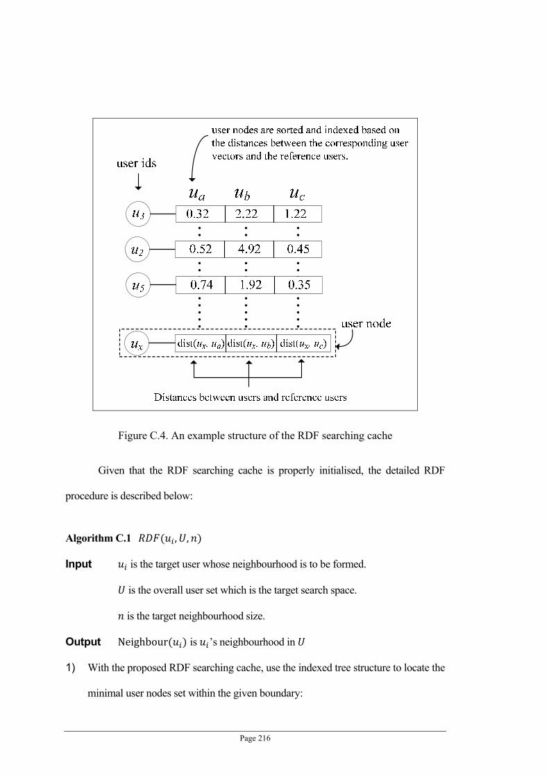
Page 216
Figure C.4. An example structure of the RDF searching cache
Given that the RDF searching cache is properly initialised, the detailed RDF
procedure is described below:
Algorithm C.1 , ,
Input is the target user whose neighbourhood is to be formed.
is the overall user set which is the target search space.
is the target neighbourhood size.
Output Neighbour is ’s neighbourhood in
1) With the proposed RDF searching cache, use the indexed tree structure to locate the
minimal user nodes set within the given boundary:

Page 217
| , | , |
where , , is one of the reference users, and is set such that the
estimated searching space is minimal. Also, it can be observed that the equation
for computing depicted here is based on Equation (C.1), and we rewrote this
equation here to accommodate the new notations used in this section for describing
the RDF searching cache.
2) Based on step 1, , , is the primary index key used for sorting and
retrieving ξ . The rest two index keys (i.e. , , \ ) are denoted as and
.
3) FOR EACH
4) IF , or | , |
THEN remove from
5) END FOR
6) Do the standard ‘best- -neighbours’ search against the estimated searching space ,
and return the result neighbourhood for (the final neighbourhood size is limited
to smaller than or equal to ).
It can be seen from line (3) to line (5) of the Algorithm C.1, the size of the
searching space is further reduced by using reference users and . This process is
similar to finding the intersected space as described in Section C.1.
C.3. EXPERIMENTS AND EVALUATION
The goal of the experiment presented in this section is to evaluate whether the
proposed RDF technique can effectively improve the recommendation performance and

Page 218
computation efficiency of recommenders. Hence, this experiment involves a standard
recommender system and a set of baseline neighbourhood formation techniques. By
observing the recommender’s performance affected by equipping it with different
neighbourhood formation techniques, we can evaluate whether the proposed RDF
technique is indeed effective.
The recommender system employed in this experiment is the Taxonomy Product
Recommender (TPR) proposed by Ziegler et al. (2004), for detailed information about
this technique please refer to Section 2.2, Section 3.3.3.1 and (Ziegler et al., 2004).
C.3.1. Data Acquisition
The dataset employed in this experiment is the ‘Book-Crossing’ dataset
(http://www.informatik.uni-freiburg.de/~cziegler/BX/) which is also the main
experiment dataset employed in Chapter 3. Please refer to Section 3.3.1 for more details
about the dataset.
Because the TPR uses only implicit user ratings, therefore, we further removed
all explicit user ratings from the dataset and kept the remaining 716,109 implicit ratings
for the experiment.
C.3.2. Experiment Framework
In order to evaluate whether the proposed RDF method is effective in improving
recommenders’ recommendation quality and computation efficiency, we implemented
four different version of TPR, and each of them is equipped with different
neighbourhood formation algorithms. The four TPR versions are:

Page 219
TPR: this is the standard TPR version, and there is no optimisation in its
neighbourhood formation process. That is, the neighbourhood formation
process involved requires comparing the target user with all other users in
the dataset.
RDF based TPR: this TPR version employs the proposed RDF method to
form the neighbourhood.
RTree based TPR: this TPR version employs the RTree (Manolopoulos et
al., 2005) technique to form the neighbourhood. RTree is a tree structure
based neighbourhood formation method, and it has been widely applied in
many applications.
Random TPR: this TPR version forms its neighbourhood with randomly
chosen users. It is used as the baseline for the recommendation quality
evaluation.
C.3.3. Evaluation Metrics
In the recommendation performance part of evaluation, the k-folding technique
(Herlocker et al., 2004) is employed (where is set to 5 in our setting). With k-folding,
every user ’s implicit rating list is divided into 5 equal size portions. With these
portions, one of them is selected as ’s training set , and the rest 4 portions are
combined into a test set \ . Totally we have five combinations , ,
1 5 for user . In the experiment, the recommenders will use the training set
to learn ’s interest, and the recommendation list generated for will then be
evaluated according to . Moreover, the size for the neighbourhood formation is set to
20 and the number of items within each recommendation list is set to 20 too.

Page 220
The metrics used in this experiment to evaluate the recommendation list (i.e. )
against the testing item list (i.e. ) are the Precision metrics and Recall metrics, for
detailed information about these two metrics please refer to Equation (3.19) and
Equation (3.20).
For the computation efficiency evaluation, the average time required by different
TPRs to make a recommendation will be compared. We incrementally increase the
number of users in the dataset (from 1000, 2000, 3000 until 14000), and observe how the
computation times are affected by the increments.
C.3.4. Experimental Results
Figure C.5 and Figure C.6 show the performance comparison between the
standard TPR and the proposed RDF based TPR using the precision and recall metrics.
The horizontal axis for both precision and recall charts indicates the minimum number of
ratings in the user’s profile (i.e.| |). Therefore, larger x-coordinates imply that fewer
users are considered for the evaluation. It can be observed that the proposed RDF based
TPR outperformed standard TPR for both recall and precision. The result confirms that
when the dissimilar users are removed from the neighbourhood, the quality of the result
recommendations become better. RTree based TPR performs much worse than both the
RDF based TPR and the standard TPR, as it is unable to accurately allocate neighbours
for target users.

Page 221
Figure C.5. Precision Results for different TPR versions
Figure C.6. Recall Results for different TPR versions
The efficiency evaluation is shown in Figure C.7. It can be seen from Figure C.7
that the time efficiency for standard TPR drops drastically when the number of users in
the dataset increases. For dataset with 15000 users, the system needs about 14 seconds to
produce a recommendation for a user, and it is not acceptable for most commercial
systems. By comparison, the RDF based TPR is much efficient, and it only needs less

Page 222
than 4 seconds to produce a recommendation for dataset with 15000 users. The RTree
based TPR greatly outperforms the proposed method when the number of users in the
dataset is under 8000. However, as the number of users increases in the dataset, the
differences between RDF and RTree based TPR becomes smaller, and RDF starts
outperforms RTree when the number of users in the dataset is over 9000. This is because
RTree is only efficient when the tree level is small. However, as the tree level increases
(i.e. when number of users increases) RTree’s performance drops drastically because the
chance for high dimensional vector comparison increases quadratically in accordance to
the number of tree level. The proposed RDF method outperforms RTree method because
its indexing strategy is single value based, and it reduces the possibility for the high
dimensional vector correlation computation.
Figure C.7. Average recommendation time for different TPR versions

Page 223
Bibliography
ADOMAVICIUS, G., SANKARANARAYANAN, R., SEN, S. & TUZHILIN, A.
(2005) Incorporating contextual information in recommender systems using a
multidimensional approach ACM Trans. Inf. Syst., 23, 103-145.
AL-DAOUD, M. D. B. (2005) A New Algorithm for Cluster Initialization. Transactions
on Engineering Computing and Technology. Istanbul, Turkey.
AROYO, L., STASH, N., WANG, Y., GORGELS, P. & RUTLEDGE, A. L. (2007)
CHIP demonstrator: semantics-driven recommendations and museum tour
generation. Semantic Web Challenge 2007. Busan, Korea.
AWERBUCH, B., PATT-SHAMIR, B., PELEG, D. & TUTTLE, M. (2005) Improved
recommendation systems. 16th annual ACM-SIAM Symposium on Discrete
algorithms. Vancouver, British Columbia.
AZOULAY-SCHWARTZ, R., KRAUS, S. & WILKENFELD, J. (2004) Exploitation vs.
exploration: choosing a supplier in an environment of incomplete information.
Decision Support Systems, 38, 1--18.
BADRUL, S., GEORGE, K., JOSEPH, K. & JOHN, R. (2001) Item-based collaborative
filtering recommendation algorithms. Proceedings of the 10th international
conference on World Wide Web. Hong Kong, Hong Kong, ACM.
BALABANOVIĆ, M. & SHOHAM, Y. (1997) Fab: content-based, collaborative
recommendation Communications of the ACM, 40, 66-72.
BASU, C., HIRSH, H. & COHEN, W. W. (1998) Recommendation as classification:
Using social and content-based information in recommendation. 5th National
Conference on Artificial Intelligence.

Page 224
BERKHIN, P. (2002) Survey Of Clustering Data Mining Techniques. San Jose, CA,
Accrue Software.
BILLSUS, D., PAZZANI, M. J. & CHEN, J. (2000) A learning agent for wireless news
access. 5th international conference on Intelligent user interfaces New Orleans,
Louisiana, United States
BILLSUS, D. & PAZZANI., M. (1999) A hybrid user model for news classification. 7th
International Conference on User Modelling. New York, Spring-Verlag.
BOONE, G. (1998) Concept features in Re:Agent, an intelligent Email agent 2nd
international conference on Autonomous agents Minneapolis, Minnesota, United
States
BREESE, J. S., HECKERMAN, D. & KADIE, C. (1998) Empirical Analysis of
Predictive Algorithms for Collaborative Filtering. Proceedings of 14th
Conference on Uncertainty in Artificial Intelligence. Madison, WI.
BURKE, R. (2002) Hybrid Recommender Systems: Survey and Experiments. User
Modeling and User-Adapted Interaction, 12, 331-370.
CASTAGNOS, S. & BOYER, A. (2007) Modeling Preferences in a Distributed
Recommender System. Lecture Notes in Computer Science. Springer Berlin /
Heidelberg.
CHEN, J. R., WOLFE, S. R. & WRAGG, S. D. (2000) A distributed multi-agent system
for collaborative information management and sharing. 9th International
Conference on Information and Knowledge Management. McLean, Virginia,
United States, ACM.
CHRISTOPH, B. (1997) A probabilistic model for distributed information retrieval. 20th
annual international ACM SIGIR conference on Research and development in
information retrieval. Philadelphia, Pennsylvania, United States, ACM.

Page 225
CLEMENTS, M., VRIES, A. P. D., POUWELSE, J. A., WANG, J. & REINDERS, M. J.
T. (2007) Evaluation of Neighbourhood Selection Methods in Decentralized
Recommendation Systems. Workshop on Large Scale Distributed Systems for
Information Retrieval Netherlands.
CLEVERDON, C. W., MILLS, J. & KEEN, M. (1966) Factors determining the
performance of indexing systems. ASLIB Cranfield project, Cranfield.
COHEN, W. W. (1995) Fast Effective Rule Induction. IN PRIEDITIS, A. & RUSSELL,
S. (Eds.) 12th International Conference on Machine Learning. Tahoe City, CA,
Morgan Kaufmann.
COHEN, W. W. (1996) Learning rules that classify e-mail. AAAI Spring Symposium on
Machine Learning in Information Access.
COOLEY, R., TAN, P.-N. & SRIVASTAVA, J. (1999) Websift: the web site
information filter system. 1999 KDD Workshop on Web Mining. San Diego, CA,
Springer-Verlag.
CÖSTER, R., GUSTAVSSON, A., OLSSON, T. & RUDSTRÖM, Å. (2002) Enhancing
web-based configuration with recommendations and cluster-based help.
Workshop on Recommendation and Personalization in eCommerce. Malaga,
Spain.
CUNNINGHAM, P., BERGMANN, R., SCHMITT, S., TRAPHÖNER, R., BREEN, S.
& SMYTH, B. (2001) WEBSELL: Intelligent Sales Assistants for the World
Wide Web. KI - Zeitschrift fr Knstliche Intelligenz.
DEGEMMIS, M., LOPS, P., SEMERARO, G., COSTABILE, M. F., GUIDA, S. P. &
LICCHELLI, O. (2004) Improving Collaborative Recommender Systems by
means of User Profiles. Human-Computer Interaction Series: Designing
personalized user experiences in eCommerce. Norwell, MA, USA, Kluwer
Academic Publishers.

Page 226
DESHPANDE, M. & KARYPIS, G. (2004) Item-based top-N recommendation
algorithms. ACM Transactions on Information Systems, 22, 143-177.
DRINEAS, P., KERENIDIS, I. & RAGHAVAN, P. (2002) Competitive
recommendation systems. 34th annual ACM symposium on Theory of computing.
New York, NY, USA, ACM Press.
FERMAN, A. M., ERRICO, J. H., BEEK, P. V. & SEZAN, M. I. (2002) Content-based
filtering and personalization using structured metadata. 2nd ACM/IEEE-CS joint
conference on Digital libraries Portland, Oregon, USA.
FONER, L. N. (1997) Yenta: a multi-agent, referral-based matchmaking system. 1st
International Conference on Autonomous agents. Marina del Rey, California,
United States, ACM.
FRENCH, J. C., POWELL, A. L., CALLAN, J. P., VILES, C. L., EMMITT, T., PREY,
K. J. & MOU, Y. (1999) Comparing the Performance of Database Selection
Algorithms. Research and Development in Information Retrieval.
FRIGUI, H. & KRISHNAPURAM, R. (1997) Clustering by competitive agglomeration.
Pattern recognition, 30, 1109-1119
FUNAKOSHI, K. & OHGURO, T. (2000) A content-based collaborative recommender
system with detailed useof evaluations. 4th Conference on Knowledge-Based
Intelligent Engineering Systems and Allied Technologies.
GHANI, R. & FANO, A. (2002) Building recommender systems using a knowledge
base of product semantics. Workshop on Recommendation and Personalization
in E-Commerce (RPEC). Malaga, Spain, Springer-Verlag.
GOLDBERG, D., NICHOLS, D., OKI, B. M. & TERRY, D. (1992) Using collaborative
filtering to weave an information tapestry. Communications of the ACM, 35, 61-
70.

Page 227
GOOD, N., SCHAFER, J. B., KONSTAN, J. A., BORCHERS, A., SARWAR, B. M.,
HERLOCKER, J. L. & RIEDL, J. (1999) Combining collaborative filtering with
personal agents for better recommendations. 6th National Conference on
Artificial Intelligence.
GUI-RONG, X., CHENXI, L., QIANG, Y., WENSI, X., HUA-JUN, Z., YONG, Y. &
ZHENG, C. (2005) Scalable collaborative filtering using cluster-based
smoothing. 28th annual international ACM SIGIR conference on research and
development in information retrieval. Salvador, Brazil, ACM.
HAN, P., XIE, B., YANG, F. & SHEN, R. (2004) A scalable P2P recommender system
based on distributed collaborative filtering. Expert Systems with Applications, 27,
203-210.
HAYES, C., MASSA, P., AVESANI, P. & CUNNINGHAM, P. (2002) An on-line
evaluation framework for recommender systems. Personalization and
Recommendation in E-Commerce. Malaga.
HERLOCKER, J., KONSTAN, J. A. & RIEDL, J. (2002) An empirical analysis of
design choices in neighborhood-based collaborative filtering algorithms.
Information Retrieval, 5, 287-310.
HERLOCKER, J. L., KONSTAN, J. A., TERVEEN, L. G. & RIEDL, J. T. (2004)
Evaluating collaborative filtering recommender systems. ACM Transactions on
Information Systems (TOIS), 22, 5-53.
HOLLINK, L., SCHREIBER, G. & WIELINGA., B. (2007) Patterns of semantic
relations to improve image content search. Journal of Web Semantics, 5, 195-203.
JAIN, A. K., MURTY, M. N. & FLYNN, P. J. (1999) Data Clustering: A Review. ACM
Computing Surveys, 31, 264-323.
JENNINGS, A. & HIGUCHI, H. (1993) A user model neural network for a personal
news service User Modeling and User-Adapted Interaction, 3, 1-25.

Page 228
JEROME, K. & DEREK, B. (2004) An accurate and scalable collaborative
recommender. Artif. Intell. Rev., 21, 193-213.
JIAN, C., JIAN, Y. & JIN, H. (2005) Automatic content-based recommendation in e-
commerce. e-Technology, e-Commerce and e-Service.
JOHN, G. (1989) Multi-armed bandit allocation indices, Wiley.
JUN, W., ARJEN, P. D. V. & MARCEL, J. T. R. (2006) Unifying user-based and item-
based collaborative filtering approaches by similarity fusion. Proceedings of the
29th annual international ACM SIGIR conference on Research and development
in information retrieval. Seattle, Washington, USA, ACM.
KARYPIS, G. (2001) Evaluation of Item-Based Top-N Recommendation Algorithms.
10th Conference of Information and Knowledge Management.
KIM, J. W., LEE, B. H., SHAW, M. J., CHANG, H.-L. & NELSON, M. (2001)
Application of decision-tree induction techniques to personalized advertisements
on internet storefronts. International Journal of Electronic Commerce 5, 45-62.
KOHRS, A. & MERIALDO, B. (2000) Using category-based collaborative filtering in
the active WebMuseum. IEEE International Conference on Multimedia and
Expo.
KONSTAN, J. A., MILLER, B. N., MALTZ, D., HERLOCKER, J. L., GORDON, L. R.
& RIEDL, J. (1997) GroupLens: applying collaborative filtering to Usenet news.
Communications of the ACM, 40, 77-87.
KRETSER, O. D., MOFFAT, A., SHIMMIN, T. & ZOBEL, J. (1998) Methodologies
for Distributed Information Retrieval. International Conference on Distributed
Computing Systems.
KRISS, S. (2007) Collaborative Filtering and the Netflix Challenge. Yale University.

Page 229
KRULWICH, B. (1997) LIFESTYLE FINDER: Intelligent User Profiling Using Large-
Scale Demographic Data. AI Magazine, 18, 37-45.
LEMIRE, D. & MACLACHLAN, A. (2005) Slope One Predictors for Online Rating-
Based Collaborative Filtering. 2005 SIAM Data Mining
LEO, O., HOWARD, H. L. & ROBERT, E. W. (2003) Ontologies for corporate web
applications. AI Mag., 24, 49-62.
LEVY, T. (2004) The state and value of taxonomy standards. The Seybold Report July
21, 2004.
LIKAS, A., VLASSIS, N. & VERBEEK, J. J. (2003) The Global K-means Clustering
Algorithm. Pattern Recognition, 36, 451-461.
LINDEN, G., SMITH, B. & YORK, J. (2003) Amazon.com recommendations: item-to-
item collaborative filtering. Internet Computing, IEEE, 7, 76-80.
LINK, H., SAIA, J., LANE, T. & LAVIOLETTE, R. A. (2005) The Impact of Social
Networks on Multi-Agent Recommender Systems. CoRR, abs/cs/0511011.
LIU, P., NIE, G., CHEN, D. & FU, Z. (2007) The Knowledge Grid Based Intelligent
Electronic Commerce Recommender Systems. IEEE International Conference
on Service-Oriented Computing and Applications. Newport Beach, CA, USA.
MALONE, T. W., GRANT, K., TURBAK, F., A.BROBST, S. & COHEN, M. D. (1987)
Intelligent information-sharing systems. Communications of the ACM, 30, 390-
402.
MANOLOPOULOS, Y., NANOPOULOS, A., PAPADOPOULOS, A. N. &
THEODORIDIS, Y. (2005) R-Trees: Theory and Applications, Springer.
MIDDLETON, S. E., ALANI, H., SHADBOLT, N. R. & DE ROURE, D. C. (2002)
Exploiting Synergy Between Ontologies and Recommender Systems. The
Semantic Web Workshop, World Wide Web Conference.

Page 230
MIDDLETON, S. E., SHADBOLT, N. R. & ROURE, D. C. D. (2004) Ontological User
Profiling in Recommender Systems. ACM Transactions on Information Systems,
22, 54-88.
MILLER, B. N., KONSTAN, J. A. & RIEDL, J. (2004) PocketLens: Toward a personal
recommender system. ACM Transactions on Information Systems, 22, 437-476.
MIN, S.-H. & HAN, I. (2005) Recommender systems using support vector machines.
International Conference on Web Engineering.
MIRA, K. & DONG-SUB, C. (2001) Collaborative filtering with automatic rating for
recommendation. IN DONG-SUB, C. (Ed. IEEE International Symposium on
Industrial Electronics.
MLADENIC, D. (1996) Personal WebWatcher: design and implementation. Technical
Report IJS-DP-7472. Pittsburgh, USA, School of Computer Science, Carnegie-
Mellon University.
MONTANER, M., LÓPEZ, B. & ROSA, J. L. D. L. (2003) A Taxonomy of
Recommender Agents on the Internet. Artificial Intelligence Review, 19, 285-330.
OGSTON, E., OVEREINDER, B., STEEN, M. V. & BRAZIER, F. (2003) A method
for decentralized clustering in large multi-agent systems. 2nd International Joint
Conference on Autonomous Agents and Multiagent Systems. Melbourne,
Australia, ACM.
PAPAGELIS, M. & PLEXOUSAKIS, D. (2004) Qualitative Analysis of User-Based
and Item-Based Prediction Algorithms for Recommendation. Lecture Notes in
Computer Science, 3191/2004, 152-166.
PAPAGELIS, M., ROUSIDIS, I. & PLEXOUSAKIS, D. (2005) Incremental
Collaborative Filtering for Highly-Scalable Recommendation Algorithms.
Proceedings of the15th International Symposium on Methodologies of Intelligent
Systems.

Page 231
PARK, S.-T., PENNOCK, D., MADANI, O., GOOD, N. & DECOSTE, D. (2006)
Naive filterbots for robust cold-start recommendations. IN PRESS, A. (Ed. 12th
ACM SIGKDD international conference on Knowledge discovery and data
mining. Philadelphia, PA, USA.
PAZZANI, M., MURAMATSU, J. & BILLSUS, D. (1996) Syskill & Webert:
Identifying interesting web sites. 13th National Conference on Artificial
Intelligence.
PAZZANI, M. J. (1999) A framework for collaborative, content-based and demographic
filtering Artificial Intelligence Review, 13, 393-408.
PAZZANI, M. J. & BILLSUS, D. (2007) Content-based recommender systems. IN
BRUSILOVSKY, P., KOBSA, A. & NEJDL, W. (Eds.) The Adaptive Web.
Berlin, Germany, Springer-Verlag.
PEDRYCZ, W. (2005) Clustering and Fuzzy Clustering. Knowledge-Based Clustering:
From Data to Information Granules. Wiley InterScience.
PELLEG, D. & MOORE, A. (1999) Accelerating Exact k-means Algorithms with
Geometric Reasoning. Knowledge Discovery and Data Mining.
PELLEG, D. & MOORE, A. (2000) X-means: Extending K-means with Efficient
Estimation of the Number of Clusters. Seventeenth International Conference on
Machine Learning. San Francisco, Morgan Kaufmann.
POPESCUL, A., UNGAR, L., PENNOCK, D. & LAWRENCE, S. (2001) Probabilistic
Models for Unified Collaborative and Content-Based Recommendation in
Sparse-Data Environments. 17th Conference on Uncertainty in Artificial
Intelligence.
PRETSCHNER, A. & GAUCH, S. (1999) Ontology based personalized search. 11th
IEEE International Conference on Tools with Artificial Intelligence. IEEE
Computer Society.

Page 232
RASHID, A. M., LAM, S. K., LAPITZ, A., KARYPIS, G. & RIEDL, J. (2006a)
ClustKNN: a highly scalable hybrid model- and memory-based CF algorithm.
Workshop on Web Mining and Web Usage Analysis. Philadelphia, Pennsylvania.
RASHID, A. M., LAM, S. K., LAPITZ, A., KARYPIS, G. & RIEDL, J. (2006b)
Towards a Scalable kNN CF Algorithm: Exploring Effective Applications of
clustering. Workshop on Web Mining and Web Usage Analysis. Philadelphia,
Pennsylvania.
RESNICK, P. & VARIAN, H. R. (1997) Recommender systems. Communications of
the ACM 40, 56--58.
RICH, E. (1998) User modeling via stereotypes. Readings in intelligent user interfaces.
San Francisco, CA, USA, Morgan Kaufmann Publishers Inc.
RUSSELL, S. & NORVIG, P. (2002) Artificial Intelligence: A Modern Approach,
Prentice.
SAITOH, S. (2003) Generalizations of the Triangle Inequalty. Journal of Inequalities in
Pure and Applied Mathematics, 4.
SALTON, G. (1983) Introduction to Modern Information Retrieval, New York,
McGraw-Hill Companies.
SARWAR, B., KARYPIS, G., KONSTAN, J. & RIEDL, J. (2000a) Application of
dimensionality reduction in recommender systems--a case study. ACM WebKDD
Workshop. Boston, MA, USA.
SARWAR, B., KARYPIS, G., KONSTAN, J. & RIEDL, J. (2002) Recommender
systems for large-scale e-commerce: Scalable neighborhood formation using
clustering. Fifth International Conference on Computer and Information
Technology.

Page 233
SARWAR, B. M., KARYPIS, G., KONSTAN, J. A. & RIEDL, J. (2000b) Analysis of
recommendation algorithms for e-commerce. ACM Conference on Electronic
Commerce.
SCHAFER, J. B., KONSTAN, J. A. & RIEDL, J. (2000) E-Commerce
Recommendation Applications. Journal of Data Mining and Knowledge
Discovery, 5, 115-152.
SCHEIN, A. I., POPESCUL, A., UNGAR, L. H. & PENNOCK, D. M. (2002) Methods
and metrics for cold-start recommendations 25th annual international ACM
SIGIR conference on Research and development in information retrieval.
Tampere, Finland, ACM Press.
SCHWAB, I., POHL, W. & KOYCHEV, I. (2000) Learning to recommend from
positive evidence. AAAI 2000 Spring Symposium: Adaptive User Interface.
SHARDANAND, U. & MAES, P. (1995) Social information filtering: algorithms for
automating word of mouth. CHI'95 Conference on Human Factors in
Computing Systems. ACM Press.
SMITH, R. G. (1981) The Contract Net Protocol: High-Level Communication and
Control in a Distributed Problem Solver. IEEE Transactions on Computers, C-
29, 1104--1113.
SOLLENBORN, M. & FUNK, P. (2002) Category-based filtering and user stereotype
cases to reduce the latency problem in recommender systems. 6th European
Conference on Advances in Case-Based Reasoning London, UK, Springer-
Verlag.
SORGE, C. (2007) A Chord-based Recommender System. 32nd IEEE Conference on
Local Computer Networks, 2007. LCN 2007. .
TABACHNICK, B. G. & FIDELL, L. S. (2006) Using Multivariate Statistics, Allyn &
Bacon.

Page 234
TERVEEN, L., HILL, W., AMENTO, B., MCDONALD, D. & CRETER, J. (1997)
PHOAKS: A system for sharing recommendations. Communications of the ACM,
40, 59-62.
TOWLE, B. & QUINN, C. (2000) Knowledge based recommender systems using
explicit user models. Knowledge-Based Electronic Markets Workshop at AAAI
2000. Austin, TX.
TVEIT, A. (2007) Peer-to-peer based Recommendations for Mobile Commerce. the
First International Workshop on Mobile Commerce. Rome, Italy.
VIDAL, J. M. V. M. (2004) A Protocol for a Distributed Recommender System.
Trusting Agents for Trusting Electronic Societies.
WANG, J., POUWELSE, J., LAGENDIJK, R. & REINDERS, M. R. J. (2006)
Distributed Collaborative Filtering for Peer-to-Peer File Sharing Systems. 21st
Annual ACM Symposium on Applied Computing.
WEI, Y. Z., MOREAU, L. & JENNINGS, N. R. (2003) Recommender Systems: A
Market-Based Design. 2nd International Joint Conference on Autonomous
Agents and Multiagent Systems. Melbourne, Australia.
WEI, Y. Z., MOREAU, L. & JENNINGS, N. R. (2005) A market-based approach to
recommender systems. ACM Transactions on Information Systems 23, 227-266.
WEISS, G. (1999) Multiagent Systems: a modern appraoch to distributed artificial
intelligence, London, England, The MIT Press.
XU, Y. (2005) Hybrid Clustering with Application to Web Mining. Active Media
Technology. Japen.
YANG, C. C., CHEN, H. & HONG, K. (2003) Visualization of large category map for
Internet browsing Decision Support Systems, 35, 89-102.

Page 235
YANG, J., WANG, J., CLEMENTS, M., POUWELSE, J. A., VRIES, A. P. D. &
REINDERS, M. (2007) An Epidemic-based P2P Recommender System.
Workshop on Large Scale Distributed Systems for Information Retrieval
Netherlands.
ZENG, C., XING, C.-X. & ZHOU, L.-Z. (2003) Similarity measure and instance
selection for collaborative filtering. Proceedings of the 12th international
conference on World Wide Web. Budapest, Hungary
ZIEGLER, C.-N. & GOLBECK, J. (2007) Investigating interactions of trust and interest
similarity. Decision Support Systems, 43, 460-475.
ZIEGLER, C.-N., LAUSEN, G. & SCHMIDT-THIEME, L. (2004) Taxonomy-driven
Computation of Product Recommendations International Conference on
Information and Knowledge Management Washington D.C., USA