Information Day 2021 Milk production from planted pastures
102
Information Day 2021 Milk production from planted pastures Outeniqua Research Farm: Directorates Plant and Animal Sciences
Transcript of Information Day 2021 Milk production from planted pastures

Information Day 2021
Milk production from planted
pastures
Outeniqua Research Farm: Directorates Plant and
Animal Sciences

2
CONTENTS
Information Day Programme 3
Foreword 4
Contact details 5
Plant Sciences– Brief overview 7
Animal Sciences– Brief overview 9
Climate-smart dairy farming: opportunities for carbon mitigation and improved
resource management 10
Tall Fescue and Festulolium cultivar evaluation results: the first 15 months 2020/21 23
Perennial ryegrass cultivar evaluation results for 2020/21 34
Italian and hybrid ryegrass cultivar evaluation results for 2020/21 51
Forage herbs (Chicory and plantain) cultivar evaluation seasonal yield results for
October 2018 to February 2021 70
The integration of forage herbs into systems: lessons learnt from farmlet studies 76
The effect of partial replacement of perennial ryegrass with plantain pasture and
concentrate level on milk production and milk composition of Jersey cows in
spring
88
Milk flocculation: Does feeding more phosphorous to cows improve milk protein
stability? 92
Weather data: Outeniqua Research Farm 2019 to 2021 95

3

4
And so another year of the COVID pandemic and associated
challenges continued amidst our hopes to move closer to one
another, socialize, de-mask and return to our normal lives.
Our research efforts continued despite COVID regulations and our
teams were working according to new routines and schedules. The
“not so normal” became normal, our walk and talks and information
days became virtual days. The word “virtual” means “being on or
simulated on a computer or computer network”, but nothing about our research was “simulated”.
Our team was out there in the pastures and the dairy! It was only technology transfer in a new
format, and the real research work was done despite the pandemic, resulting in advancements
for dairy farmers at all levels.
In the past year the agricultural sector was challenged on many other levels as well, including
climate change and farming in a climate smart way to ensure sustainability and resource
optimisation. The research portfolio of the Western Cape Department is problem focused and farmer
driven and we are committed to continue our support to our farmers, and in particular the farmers in
the Southern Cape. We have also extended our impact with innovative tools like drone technology,
spatial decision making tools and smart sensors, to name but a few. We are proud to announce that
we could fill all our vacancies with skilled persons, the latest being two young animal scientists who
joined the team of the Directorate Animal Sciences.
This year our well known Outeniqua information day is again virtually presented by a dedicated
pasture and dairy research team who are not only experts in their respective fields, but who also
know the researcher-farmer interface very well.
Please enjoy the day with us from a venue of your choice – be safe and be healthy!
Dr. Ilse Trautmann
Chief Director: Research and Technology Development Services
FOREWORD

5
CONTACT DETAILS
Dr Ilse Trautmann
Chief Director: Research and Technology Development
Department of Agriculture
Western Cape Government
Prof Robin Meeske
Specialist Scientist: Animal Science
Directorate Animal Science
Department of Agriculture
Western Cape Government
Tel: 044 803 3708 Cell no: 082 908 4110
Sigrun Ammann
Scientist: Pastures
Directorate Plant Science
Department of Agriculture
Western Cape Government
Tel: 044 803 3726 Cell no: 082 775 8836
Janke van der Colf
Scientist: Pasture Systems
Directorate Plant Science
Department of Agriculture
Western Cape Government
Tel: 044 803 3716 Cell no: 082 774 9164

6
CONTACT DETAILS
Prof Stephanie J.E. Midgley
Research and Technology Development Services
Department of Agriculture
Western Cape Government
Tel: (021) 808 5080
Annelene Swanepoel
Scientific Manager: Directorate Plant Sciences
Research & Technology Development Services
Department of Agriculture
Western Cape Government
Tel: (021) 808 5320
Chris de Brouwer
Scientific Manager: Directorate Animal Sciences
Research & Technology Development Services
Department of Agriculture
Western Cape Government
Tel: (021) 808 5220 Cell no: 082 3398547

7
PLANT SCIENCES – A BRIEF OVERVIEW
Annelene Swanepoel
Western Cape Department of Agriculture, Research and Technology Development, Directorate Plant Sciences
Corresponding author email: [email protected]
Research in the Directorate has been organised into
various research programmes in order to focus on
specific disciplines. Sustainability, conservation
agriculture, conservation of resources,
environmental impact, and lower input cost are
golden threads throughout the projects, and
climate smart agriculture is incorporated as
technologies develop.
Research on veld and natural pastures is currently
focused on rehabilitation of degraded areas,
management of invasive species, veld monitoring,
as well as seed production of indigenous species for
arid areas. We also support drought risk
management with scientific inputs where required.
Sustainable production and crop rotation systems
research is conducted mainly in the cropping areas
of the Swartland and southern Cape. It is one of our
flagship programmes and provides information on
new cultivation practices and the biological and
economical effects of these systems. It also creates
opportunities for post graduate students and other
researchers in agriculture (Universities, ARC, etc.) to
do component/basic research within these systems
trials and optimising the knowledge gained from
these trials. New research focuses specifically on
Conservation Agriculture (CA) production systems,
with attention to specific knowledge gaps within
these production systems for farm level efficiency.
We also provide the secretariat for the association
“Conservation Agriculture Western Cape”.
Pasture systems research, including evaluation and
introduction of new species and varieties and also
pasture system management, is mainly focused on
irrigated pasture systems for dairy and, to a lesser
degree on dry-land pastures for the cropping areas
of the Swartland and southern Cape. The driving
force for sustainable dairy production from irrigated
pastures is the research group at Outeniqua
Research Farm at George, where the only research
of its kind in the country is executed. They focus on
the development of sustainable dairy production
systems, from soil to pasture crops to grazing
management and milk yield and quality, within
sustainability and economic parameters. The Plant
Sciences group is responsible for the soil and plant
sciences part of the research, with collaboration on
grazing management research, from the Animal
Sciences directorate. This group also present
pasture courses to farmers and advisors in the dairy
and seed industries.
Grain, oil- and protein seed crops form the basis of
small grain cropping enterprises and this programme
focuses on evaluation of suitable varieties for our
province, as well as the best cultivation and
management practices for these crops, whether it is
a cash crop or a cover crop.
Research on soil, plant and water management has
been expanded, specifically pertaining to the
biological component of the soil. Conservation
agriculture practices have also demanded new
research around fertiliser norms and extensive long-
term trials on soil fertility, fertiliser requirements and
tillage practices are being executed.
Priority areas that are also currently being expanded

8
are Alternative crops, in view of the expected
impact of climate change and Vegetables,
particularly pertaining to the subsistence- and
smallholder farmers in our province. This is crucial in
addressing food security in the province, as well as
maximising outputs and profit for producers on small
areas of land.
Supporting all these programmes as set out above, is
expertise in the fields of entomology, plant
pathology and weed science, as well as our
analytical laboratory for soil, plant and water
analyses and our diagnostic laboratory for plant
diseases. These programmes support and enhance
all research within the Directorate, from veld,
pastures, crops and alternative crops to vegetables,
addressing areas of expertise that is not limited only
to specific crops, but integrated through the various
production systems. Extensive research is being
done on a range of crops and within various systems
trials to address pertinent production issues,
including international collaboration, in particular in
the field of plant pathology. Also, the analytical and
diagnostic laboratories offer analytical services to
the public, who can request analyses of soil, plant
and water samples at a reasonable cost.
Recently, we have also started developing new
technology around remote sensing and crop
management and aim to develop those into useful
support systems for our producers in order to
continue to grow agriculture in the Western Cape.

9
ANIMAL SCIENCES – A BRIEF OVERVIEW
Dr Chris de Brouwer
Western Cape Department of Agriculture, Research and Technology Development, Directorate Animal
Sciences
Corresponding author email: [email protected]
The Animal Science Directorate has the mandate to
research livestock production in the Western Cape.
The purpose of the Directorate is to address industry
challenges through needs-based animal production
research. Needs identification happens through
industry engagement and linkages with the
Programe Agricultural Producers’ Support and
Developments in the department.
In terms of research resources the Directorate is
conducting research on 6 research farms that are
spread over the province. They are Elsenburg
(Stellenbosch), Langgewens (Moorreesburg), Nortier
(Lamberts Bay), Tygerhoek (Riviersonderend),
Outeniqua (George) and Oudsthoorn.
The focus is divided into nutrition/products and
breeding/genetics research.
The research commodities are:
1. Small stock including Merino, SAMM, Dormer
and indigenous (Namakwa Afrikaner) and
composites breeds (Dorper and Meatmaster).
Wool
Meat – mutton and lamb
Nutrition
Growth modelling
Ideal slaughter weight
Genetics and genomics
2. Dairy cattle in total mixed ration (Holstein) and
pasture-based systems (Jersey),
Milk yield
Milk quality (butterfat, protein, etc.)
Feed cost saving, both in TMR and
grazing systems
Improved feed utilisation, and
3. Ostriches (SA Black, Zimbabwe Blue and
Kenyan Red).
Breeding and crossbreeding,
Development of breeding values for
important production parameters,
Hatchability and chick survival,
Value add through heavier carcasses,
sought after leather traits
Improved growth performance
A team of nine researchers who work in tandem with
eleven research technicians, with support, in turn,
from foremen, auxiliary officers and farm aids
conducts the research.
The research portfolio comprises an average of 38
projects at any given time. The projects investigate
all aspects of animal production regarding nutrition,
products, breeding and genetics in the commodities
mentioned.

10
Climate-smart dairy farming: opportunities for carbon
mitigation and improved resource management
Prof Stephanie J.E. Midgley
Research and Technology Development Services, Western Cape Department of Agriculture
Corresponding author email: [email protected]
Introduction
The agricultural sector of South Africa and of the
Western Cape Province is already experiencing the
impacts of human-driven climate change (Midgley
et al., 2016a). These impacts are placing pressure on
dairy farming in interaction with rising economic and
social pressures, pressures arising from the
degradation of the natural resources base in many
regions, and the deterioration of air and water
quality. Across the globe and in all sectors, there is a
heightened urgency to intervene in order to limit the
extent and impact of future climatic changes by
rapidly reducing the sources and enhancing the
sinks of greenhouse gases (GHGs) (termed climate
change mitigation) (IPCC, 2021). A sink can be any
activity or mechanism that removes GHGs from the
atmosphere, such as the fixing of atmospheric
carbon dioxide (CO2) by plants through
photosynthesis and its long-term storage in the soil
carbon pool, termed carbon sequestration. Pasture-
based dairy production has a significant footprint
resulting from intensive energy, water and fertiliser
use. Nevertheless, it offers several opportunities for
cost-effective reductions in emissions of key GHGs,
and for meaningful and even profitable carbon
sequestration interventions.
Simultaneously, climate change will have
disproportionately high negative impacts on
pastures that are in a degraded state, and where
soil and water resources are poorly or sub-optimally
managed. Across South Africa and the Western
Cape, water is a scarce and precious resource, and
climate change is projected to lead to changes in
rainfall amounts and seasonal rainfall patterns,
which, together with rising temperatures, will reduce
the water supply available to agriculture, and
increase the rate of soil drying between rainfall/
irrigation events (DEFF, 2019). Excessive applications
of nutrients and poor manure management,
degraded river and wetland systems, and other
factors in the dairy value chain, can impair the
quality of downstream and ground water resources
(Botha, 2011/2012). An array of adaptive strategies
and better practices is available for addressing the
actual or expected climate effects on water
resources while in many instances reducing input
costs.
One of the manifestations of climate change that
has recently become highly visible both globally
and locally is the increasing frequency, intensity and
duration of extreme rainfall events such as droughts
and floods (Otto et al., 2018; CSIR 2021 https://
greenbook.co.za/). Managed pastures are highly
vulnerable to these extremes, particularly in areas
without sufficient water storage or well designed
drainage infrastructure. This is an area of concern
that has not received the same level of interest from
the dairy sector as GHG emissions and
environmental sustainability. Mitigation of disaster risk

11
is needed to lessen the potential adverse impacts
on farms and regions.
This paper focuses on the farm level, with emphasis
on pasture management, notwithstanding the
important impacts on, and role of the cows and the
whole dairy value chain. These have been
discussed in several previous publications (Botha,
2011/2012; Midgley, 2015). The aim here is to provide
a science-based summary of the following
considerations, in the context of three dairy regions
of the Western Cape. Recommendations for further
research are provided.
1. Overview of climate change trends and
projections
2. Opportunities to reduce GHG (CO2, nitrous
oxide [N2O]) emissions from pasture-based
dairy farming (excluding the role of enteric
fermentation and methane [CH4] emissions);
3. Opportunities to sequester carbon in pasture
soils;
4. Protection and efficient use of water
resources.
Overview of climate change trends and projections
Three major dairy production regions of the Western
Cape will be assessed: the western region,
Overberg, and southern Cape (Fig. 1). These coastal
regions are characterised by lower annual rainfall in
the Western and Overberg regions and higher
rainfall in the southern Cape (Fig. 2 top left), a west-
east shift in rainfall seasonality from winter rainfall to
all-year rainfall (Fig. 2 top right), a relatively similar
mean annual temperature (16-18°C, Fig. 2 bottom)
and cool winters, but hotter summer days in most of
the western region compared to the Overberg and
southern Cape. This diversity results in a matrix of
expected future climates once the modelled
climate change projections are overlaid. It is
important to note that dairy production occurs in
widely differing environments and production
systems, so that climate change will affect farms in
various ways depending on the local context, and
responses must be tailored to each situation to
ensure environmental sustainability and economic
viability of the enterprise (Midgley et al., 2016b).
Figure 1. Three main dairy production regions of the Western Cape: Western, Overberg and southern
Cape. Background map: Agro-ecological Zones of the Western Cape (M. Wallace, Western Cape
Department of Agriculture).

12
Figure 2. Top left: Mean annual precipitation of the Western Cape overlaid on the Agro-ecological Zones.
Source: Midgley et al. (2016a). Top right: Rainfall seasonality of South Africa. Source: Schulze and Maharaj
(2008). Bottom: Mean annual temperature of the Western Cape. Source: Midgley et al. (2021).
Across the Western Cape, the climate is already
changing through increasingly variable and
unpredictable weather, significant rates of warming,
and more frequent climate-related extremes and
disasters (Midgley et al., 2016a; DEA, 2018).
Temperatures have increased by more than 1.1°C
on average over the last eighty years, and this trend
is especially significant in the western region. Daily
maximum temperatures and the number of hot days
are rising. Data indicates an increase in the
probability of heavy rainfall events, but fewer rain
days in late summer to autumn, and more rain days
in November-December in the west. No significant
trends in total annual rainfall can yet be discerned,
except for a moderate long-term positive trend in
the Little Karoo (in the northernmost part of the
southern Cape region) associated with summer
rainfall.
Climatologists are in agreement that shifts in climate
systems are expected over the next few decades.
Importantly for the coastal dairy regions, a
southward (poleward) shift of the westerly winds will
increasingly block the movement of rain-bringing
cold fronts making landfall (DEA, 2018). In the shorter
term (20-30 years), these shifts will emerge as
increasing inter- and intra-annual rainfall variability.
Although the projected changes in rainfall are more
uncertain than those for temperature, there is
scientific consensus that the Western Cape will
become relatively drier in the longer term as the
climate system adjusts (DEA, 2018; IPCC, 2021).
Reductions in winter rainfall are projected for most
parts of the province, but with greater certainty in
the western core winter rainfall region (Fig. 3). The
recently published first part of the sixth assessment
report on climate change of the Intergovernmental
Panel on Climate Change (IPCC, 2021) reports with
increased scientific confidence that the
Mediterranean-type climate regions of the world will
experience reductions in winter rainfall. These
regions are amongst those expected to experience
increasing aridity and agricultural and ecological
droughts under future warming (Fig. 4). In the
Western Cape, local topography is likely to

13
moderate this, and there is a possibility that more
rain could fall on windward mountain slopes in
autumn and spring, at least in the short term future,
and especially for future scenarios where global
GHG emissions are rapidly reduced (Midgley et al.,
2016a). The models also project that the current
trend towards fewer rain days and more intense
rainfall events will continue.
The global climate models are in high agreement
that warming will continue into the future, with
absolute increases depending on how successfully
the nations can achieve zero net carbon emissions.
For the Western Cape (Midgley et al., 2016a), the
projections indicate a warming of 1.5°C - 3°C by the
mid-century (Fig. 5). The lower range of warming (1.5
- 2.1°C) is expected along coast from Cape Town
eastwards, but a mid-range warming (2.1 - 2.4°C) is
expected along the west coast. In all regions, there
will be more hot days and nights, and fewer cold
days and nights.
Figure 3. Projected (modelled) changes in mean annual precipitation in the Western Cape expressed in mm (left) and
as a percentage (right) between the period 1990s and the period 2030s. The maps are derived from as yet
unpublished outputs of seven bias-corrected CMIP5 GCMs (CWWR, 2021; unpublished). Source: Midgley et al. (2021).
Figure 4. Schematic map highlighting in brown the regions where droughts are expected to become worse as a result
of climate change. This pattern is similar regardless of the emissions scenario; however, the magnitude of change
increases under higher emissions. Source: IPCC AR6 WGI FAQ 8.3, Figure 1 (IPCC, 2021).

14
A picture thus emerges of the following likely future conditions in the three dairy regions:
Figure 5. Projected (modelled) changes in mean annual temperature (in °C) from the historical climatic conditions
(1950-1999) to the intermediate future (2046-2065) in the Western Cape. The results are derived from six CMIP3 GCMs.
Source: Midgley et al. (2021); (original research: Schulze, 2011).
Table 1. Summary of projected likely future climate conditions in the three dairy regions of the Western Cape.
Region Temperature Rainfall General
Western Stronger warming and
more very hot days
Drying; reductions in winter
rainfall across the region
Increases in aridity, agricultural
and ecological drought;
increases in wind speeds;
increases in fire weather
conditions
Overberg Moderate warming and
more hot days
Drying; linked to reductions in
winter rainfall (more so in the
west) and warming, but
uncertainty about shifts in total
annual and seasonal rainfall in
the east
Increases in aridity, agricultural
and ecological drought;
increases in wind speeds;
increases in fire weather
conditions
Southern Cape Moderate warming and
more hot days
Drying linked to variable rainfall
and warming, but uncertainty
about shifts in total annual and
seasonal rainfall; some models
indicate possible minor wetting
in the shorter term in the west
Increases in aridity, agricultural
and ecological drought;
increases in heavy rainfall and
flash flooding; increases in wind
speeds; increases in fire weather
conditions

15
Figure 6. Schematic of pathways of climate change impacts on dairy production systems. Source: Author.
The impacts of these changes on pasture-based
dairy production systems will manifest via three
main pathways (Fig. 6):
1. Impacts on pasture productivity and
quality;
2. Direct impacts on animal growth, milk
production and health; and
3. Impacts of extreme weather events.
While research has significantly increased our
understanding of some of these impacts, notably
heat and nutrition stress effects on cows
(Nesamvuni et al., 2012; Du Preez, 2014), many
questions remain in other impact areas e.g. long-
term shifts in pasture production potential, changes
in the length of the growing season for pastures, the
effects of rising atmospheric CO2 concentrations on
pasture species, the rising water demand of
pastures, impacts of soil warming on soil biological
activity and GHG emissions, and the potential
impacts of more severe droughts and floods. These
require further targeted research. For now, this
paper will highlight actions that can already be
taken now based on the current knowledge base
and available improved practices and
technologies. Both adaptation (water resources)
and mitigation (pasture-based GHG emissions
reductions and carbon sequestration) will be
covered.
Opportunities to reduce GHG emissions from
pasture-based dairy farming
South Africa is the 15th-largest emitter of
greenhouse gases per capita in the world. This calls
for shared responsibility in addressing the crisis.
Estimates of direct CH4 and N2O emissions of South
African dairy and beef cattle were published by du
Toit et al. (2013). The latest National GHG Inventory
for South Africa (DEFF, 2020), based on data until
2017 and using the IPCC accounting methodology
(IPCC, 2006), highlights the high contribution of
livestock CH4 emissions and N2O emissions from
managed soil (Table 2). The global warming
potential of CH4 is 28 times that of CO2, and the
warming potential of N2O is 265 times that of CO2
over 100 years. When converted to CO2-equivalent
units, CH4 emissions from enteric fermentation by
cattle rank as the 7th (3.76%) highest contributor to
national emissions, and those from direct N2O
emissions from managed lands are the 8th highest
(3.15%) (Table 2). The total contribution by
agriculture, when all GHGs are expressed as CO2-
equivalents, is about 9% (Fig. 7 top left) and has
been a relatively constant proportion since 2000.
These figures do not include the emissions arising
from the use of electricity and liquid fuel in the dairy
value chain.

16
Opportunities to reduce GHG
emissions from pasture-based dairy
farming
South Africa is the 15th-largest emitter of greenhouse
gases per capita in the world. This calls for shared
responsibility in addressing the crisis. Estimates of
direct CH4 and N2O emissions of South African dairy
and beef cattle were published by du Toit et al.
(2013). The latest National GHG Inventory for South
Africa (DEFF, 2020), based on data until 2017 and
using the IPCC accounting methodology (IPCC,
2006), highlights the high contribution of livestock
CH4 emissions and N2O emissions from managed soil
(Table 2). The global warming potential of CH4 is 28
times that of CO2, and the warming potential of N2O
is 265 times that of CO2 over 100 years. When
converted to CO2-equivalent units, CH4 emissions
from enteric fermentation by cattle rank as the 7th
(3.76%) highest contributor to national emissions,
and those from direct N2O emissions from managed
lands are the 8th highest (3.15%) (Table 2). The total
contribution by agriculture, when all GHGs are
expressed as CO2-equivalents, is about 9% (Fig. 7 top
left) and has been a relatively constant proportion
since 2000. These figures do not include the
emissions arising from the use of electricity and liquid
fuel in the dairy value chain.
Table 2. Top eight categories for South Africa for 2017 (excluding FOLU) determined by level (L1) assessment. Source:
DEFF (2020). Emissions are expressed as gigatons of CO2-equivalents. The red block highlights the contributions of
livestock methane emissions (cattle enteric fermentation) and direct nitrous oxide emissions from managed (fertilised)
soils.
Fig. 7 shows the breakdown of emissions between
the sectors energy; industry (IPPU); AFOLU
(Agriculture, Forestry and Other Land Uses) but
excluding the FOLU component; and waste. The
negligible CO2 emissions from agriculture (0.3%)
compared to energy (92%) is particularly noteworthy
(Fig. 7 top right). CO2 emissions in agriculture (excl.
energy and fuel use) occur primarily through land-
use change.
Regarding CH4 emissions (Fig. 7 bottom left), enteric
fermentation by livestock contributed around 52% to
the national total in 2017, but the contribution from
livestock declined by 11.0% from 2000 to 2017 due to
a decline in livestock populations. The dairy cattle
contribution to the overall enteric fermentation
emissions stands at around 12%, and increased by
1.7% between 2000 and 2017.
National N2O emissions are dominated by the
contribution from agriculture (Fig. 7 bottom right),
specifically managed soils and biomass burning
(85% in 2017). This is a significant fraction of non-
carbon emissions from agriculture. However, over
the period 2000 to 2017, overall N2O emissions
declined by 10%. Livestock manure, urine and dung
inputs to managed soils provided the largest N2O
contribution in the agriculture sector and the
downward trend follows a similar pattern to the
livestock population. However, the dairy cattle
population has shown a slight uptick and thus its
contribution to N2O emissions has also risen slightly.
Regarding N2O emissions from managed land, these

17
Fig
ure
7.
Se
cto
ral c
on
trib
utio
n t
o t
he
tre
nd
in t
he
gro
ss e
mis
sio
ns
(CO
2 e
qu
iva
len
ts)
for
So
uth
Afr
ica
, 2
000
– 2
017 (
top
left
). T
ren
d a
nd
se
cto
ral c
on
trib
utio
n t
o C
O2
em
issi
on
s
(to
p r
igh
t), C
H4 e
mis
sio
ns
(bo
tto
m le
ft)
an
d N
2O
em
issi
on
s (b
ott
om
rig
ht)
fo
r th
e p
erio
d 2
00
0 –
201
7. Th
e a
gric
ultu
re s
ec
tor
(AFO
LU e
xc
l. FO
LU)
is in
dic
ate
d in
ye
llow
. So
urc
e:
DEFF (
20
20
).

18
have decreased by around 10% (direct emissions,
the dominant source) and by 9% (indirect emissions).
N2O emissions from land arise primarily from N-based
fertilizer use in intensive cultivation.
The results of the National GHG Inventory for South
Africa are, however, based on global emissions
factors, and adjustments in the results can be
expected as future updated inventory analyses use
region-specific emission factors for dairy farming
(Smit et al., 2020). Furthermore, different dairy
production systems are associated with widely
ranging GHG emissions (Reinecke and Casey, 2017)
and this will affect regional estimates.
A forward-thinking and pre-emptive approach to
climate change mitigation is required in the
agricultural sector. There remains a window of
opportunity for the dairy sector to establish farm-
level emissions baselines and emissions reductions
targets, supported by research and shifts to
practices that yield rapid emissions reductions that
are meaningful in the national emissions context
and cost-effective at farm level. Measurable and
verifiable emissions reductions will provide a bulwark
against mounting pressure on agriculture, and
livestock production systems in particular. Given the
above figures, the two areas of greatest concern
but also of greatest opportunity for the dairy sector
are CH4 and N2O emissions. Farm-based research on
coastal dairy farms confirms that CH4 from enteric
fermentation is the largest contributor of GHG
emissions, followed by N2O emissions from grazed
pastures (Galloway, et al., 2018; Smit et al., 2021).
Much research attention has focused on
technologies and practices to reduce CH4 emissions
from enteric fermentation, and this will be not be
discussed here.
Direct N2O emissions result from several pathways of
nitrogen inputs to agricultural soils (IPCC, 2006). The
following two pathways relate to farming practices
(other pathways include soil organic matter lost from
mineral soils through land-use change, and organic
soil that is drained or managed for agricultural
purposes).
Nitrogen inputs:
Synthetic nitrogen fertilizers;
Organic fertilizers (including animal
manure, compost and sewage sludge);
Crop residue (including nitrogen fixing
crops);
Animal manure deposited on pastures,
rangelands and paddocks.
Reducing emissions from the first pathway, and
specifically purchased synthetic nitrogen fertilizers, is
a relatively low-hanging fruit in most situations.
Research conducted in the western part of the
Eastern Cape found that excessive application of
nitrogen-based fertilizer and low nitrogen-use
efficiency (NUE, the percentage of N imported that
is removed in milk or animals leaving the farm) is
common in dairy farming (Galloway et al., 2018).
The average on-farm NUE in this study was 29%, and
an excess N of 284 kg/ha/year was generated.
Mineral fertilizer was the largest source of imported
N. Galloway et al. (2018) also reported a negative
correlation between NUE and GHG emission
intensity.
In a study of N2O emissions from fertilized and
irrigated dairy pastures in the southern Cape (Smit et
al., 2020), an exponential relationship was reported
between N2O nitrogen losses and N input from
fertilizer. Excessive fertilization of pastures with N
raised N2O emissions significantly, with no additional
benefit to growth of the pasture herbage. Low rates
of fertilizer application resulted in the lowest carbon
footprint (Smit et al., 2021).
Raising and optimising NUE should thus be aimed for,
using effective and affordable fertilization and
feeding strategies. These could include, in
conjunction with minimal N fertilizer application rates
(from Galloway et al., 2018; Smit et al., 2020; Smit et
al., 2021):
Minimal use of purchased
concentrates, and using those that
lead to more efficient feed conversion;
Milk production per hectare optimised
for highest NUE;
Stocking rates optimised for highest
NUE;
Rotational grazing management;
Consider the contribution of excreta to
the N balance and fertilization strategy;
Optimal timing of fertilizer application;

19
Incorporation of forage N-fixing
legumes;
Improved irrigation systems;
Increased soil carbon levels (see next
section).
Opportunities to sequester carbon in
pasture soils
While reducing GHG emissions from dairy pastures
using the above listed strategies, adapted pasture
management practices aimed at building up soil
carbon concentrations can also contribute
substantially to reducing CO2 levels in the
atmosphere, as well as improving the soil health and
water holding capacity (see next section). The
uptake and capturing of CO2 from the atmosphere
through photosynthesis, followed by the long-term
incorporation of carbon-rich compounds into the
soil, is termed carbon sequestration. It can be
accelerated through changes in agricultural
practices. Soil carbon is positively correlated with
NUE and negatively correlated with GHG emissions
(Galloway et al., 2018). Building the soil carbon levels
also leads to opportunities to reduce N fertilizer
application rates. A managed dairy pasture in the
southern Cape was found to sequester 850 – 1140 kg
C/ha/year, representing an average reduction of
14% in the carbon footprint (Smit et al., 2021).
Several strategies are available for increasing soil
organic carbon:
Applying the principles of conservation
agriculture (CA) to managed pastures, i.e.
Minimal soil disturbance, preferably using
no-till, and leaving residues to be
incorporated into the soil (no burning);
Keeping the soil surface covered with
organic material at all times (this also
reduces soil temperature which affects
carbon losses);
Using forage rotations (see Loges et al.,
2018) and a greater diversity of forage
species including nitrogen-fixing
legumes;
Including perennial grasses and other
perennial forage species in the pasture
species mix, including those with deep
root systems, to increase the long-lived
below ground biomass fraction and
exudation of carbon compounds at
greater depth;
Optimise forage growth and biomass per
hectare without excessive fertilizer
applications or irrigation;
Multi-paddock rotational grazing at a high
stocking density with periods of rest to allow for
regrowth (although the evidence is mixed, see
Contosta et al., 2021).
A study by Kirschbaum et al. (2017) does, however,
emphasise that building soil carbon is a complex
outcome of several interacting factors, including
carbon gain through higher primary production,
carbon lost through grazing and eventual milk
production, the stability of the various carbon
fractions in the soil, and changes in SOC
decomposition rates. These trade-offs are also
significantly influenced by fertilizer rates,
supplemental feed rates, soil water availability,
root:shoot ratios and soil temperature.
Carbon offset programmes have become the focus
of high interest in the agricultural community. The
principle is that farmers receive a direct financial
benefit in the form of carbon credit income, in return
for long-term carbon fixation from the atmosphere
and accumulation in farm soils. Such programmes
have recently become available in South Africa and
provide a sound opportunity for farmers to shift to
climate-friendly practices and contribute further to
GHG reductions. It must, however, be noted that
interventions must be additional to existing practices
and not business-as-usual, farmers must be able to
provide existing soil data over several years, and the
additionally fixed carbon must persist over the long
term (many decades) and in a stable form that is
protected from rapid decomposition. Dairy farmers
are encouraged to investigate such opportunities,
but are cautioned to use only programmes listed
under an internationally recognised carbon
standard.
Ultimately, the goal in agriculture is to strive towards
"net zero carbon" or even a positive balance, where
carbon sequestration is equal to or greater than
total GHG emissions.

20
Protection and efficient use of water resources
In the section on climate change trends and
projections, changes in rainfall together with
warming and greater risks of droughts were
discussed. The Western Cape already experiences
high variability in rainfall, with regions like the
southern Cape particularly prone to cycles of very
dry and very wet weather (Midgley et al., 2016a).
Climate change model outcomes send a strong
message that rainfall variability and unpredictability
are likely to worsen, and that the gap between
water supply and water demand will grow. Surface
water resources are under increasing pressure, and
groundwater resources are increasingly being used
for agriculture (especially since the 2015-2018
drought). Without improved monitoring and
management, this resource is also facing future
threats resulting from over-extraction and
salinization.
Deteriorating water quality is a major risk to humans
and agriculture. Various pathways exist through
which climate change could worsen this problem.
Intensively managed dairy pastures, especially those
with a history of excessive fertilization and poor
manure management, are sometimes part of this
problem. Nitrogen and phosphorus leaching into
surface and groundwater are especially
challenging.
The three dairy farming regions do not benefit from
large water storage capacity and irrigated pastures
receive water mainly from smaller farm dams and
rivers. Across the Western Cape, the engineered
water infrastructure is reaching its limits. Adaptation
to climate change must, therefore, focus on an
increase in agricultural water use efficiency, and
improved catchment and river management
(Midgley et al., 2016b). Significant water resources
can be released through the clearing of invasive
alien plants and the restoration of sensitive wetlands
that play a critical role in hydrological processes. This
approach is based on utilizing ecological
infrastructure, a much more cost-effective method
compared to engineered solutions. Healthy
ecological infrastructure, together with well
designed on-farm drainage infrastructure, is also
capable of mitigating the impacts of more frequent
and intense rainfall and flash flooding, as expected
in some regions in the future.
Irrigation in combination with fertilizers is used on
pasture-based dairy farms to boost forage growth
and yield, and milk production (Truter et al., 2016).
Where rainfall is insufficient or during dry periods,
supplemental irrigation is used, but many producers
have permanent systems installed. However, above
a certain optimum both inputs rapidly increase the
N2O emissions from the pasture (Smit et al., 2020).
During the warm seasons, water inputs trigger high
rates of N-mineralization, leading to large N2O fluxes.
From both an emissions and a water scarcity and
water quality point of view, the implementation of
best practices for nutrient and irrigation
management is becoming increasingly important.

21
Irrigation strategies are an important component of
climate-smart dairy farming. These can include:
Reducing total irrigation water volumes but
with shorter and more frequent application
events;
More water-efficient irrigation systems such as
drip, sub-drip and even micro irrigation;
Follow irrigation guidelines for the pasture mix,
soil type and region (Truter et al., 2016);
Where feasible use drought resilient species in
the pasture mix and those with deeper root
systems;
Install soil moisture monitoring systems to guide
irrigation scheduling; use remote precision
irrigation tools e.g. FruitLook, drones;
Aim to measure and increase the water
productivity of milk production – in addition to
Rand/liter milk and liters milk/hectare, also
monitor Rand/liter water used and liters milk/
liter water used;
Increase the soil water-holding capacity
where this is sub-optimal (see section above
on carbon sequestration) and reduce
evaporation from soils through sufficient cover
(CA principles);
Protect the water resource from wasteful losses
(e.g. leaking and faulty infrastructure) and
pollution (e.g. effluent, excess nutrients);
Install additional on-farm water storage
capacity, where possible;
Have access to more than one source of
freshwater;
Recycle and re-use waste water for irrigation;
Clear invasive alien plants along watercourses
and wetlands and maintain them alien-free;
Maintain the proper buffer zones between
managed pastures and watercourses/
wetlands;
Ensure that drainage infrastructure is well-
designed and fit for purpose under high
rainfall.
Summary
This paper has addressed three of the key
components of climate smart dairy production in
the Western Cape and highlighted several
opportunities. The cost-effectiveness of specific
interventions is highly region- and farm-specific and
requires investigation on a case-by-case basis.
However, several of the interventions are linked to
reductions in costly inputs rather than investments
that require a return on income. Consideration
should also be given to the long-term ramifications
of possible future punitive measures taken by nations
and markets (driven by consumer concerns) in their
responses to the global climate crisis, with mounting
pressure on sectors that are perceived to be high
contributors. The dairy sector will ensure resilience
and growth if it can proactively shift to practices
with measurable environmental and climate
benefits within the next 5-10 years.
References
Botha, M., 2011/2012. Dairy Sustainability: Ten
Environmental Considerations. High impact
responses to achieve low environmental impact
dairy production. WWF-SA, Newlands, South Africa.
Contosta, A.R., Arndt, K.A., Campbell, E.E., Grandy, A.S.,
Perry, A., Varner, R.K. 2021. Management intensive
grazing on New England dairy farms enhances soil
nitrogen stocks and elevates soil nitrous oxide
emissions without increasing soil carbon. Agriculture,
Ecosystems and Environment 317 (2021) 107471.
DEA, 2018. South Africa's Third National Communication
under the United Nations Framework Convention on
Climate Change. Department of Environmental
Affairs, Pretoria, South Africa.
DEFF, 2019. National Climate Change Adaptation
Strategy, Republic of South Africa. Department of
Environment, Forestry and Fisheries, Pretoria, South
Africa.
DEFF, 2020. Draft 7th National Greenhouse Gas Inventory
Report for the Republic of South Africa for Public
Comment. Government Gazette, 11 September
2020. Department of Environment, Forestry and
Fisheries, Pretoria, South Africa.
Du Preez, J. 2014. Hitte-stres. The Dairy Mail, October
2014, pp. 42–51.
Du Toit, C.J.L., Meissner, H.H., van Niekerk, W.A. 2013.
Direct methane and nitrous oxide emissions of South
African dairy and beef cattle. South African Journal
of Animal Sciences 43(3): 320–339.
Galloway, C., Conradie, B., Prozesky, H., Esler, K. 2018.
Opportunities to improve sustainability on

22
commercial pasture-based dairy farms by assessing
environmental impact. Agricultural Systems 166: 1-9.
IPCC, 2006. 2006 IPCC Guidelines for National Greenhouse
Gas Inventories. The National Greenhouse Gas
Inventories Programme, Eggleston H S, Buenida L,
Miwa K, Ngara T, and Tanabe K, eds; Institute for
Global Environmental Strategies (IGES). Hayama,
Kanagawa, Japan.
IPCC, 2021. Summary for Policymakers. In: Climate
Change 2021: The Physical Science Basis.
Contribution of Working Group I to the Sixth
Assessment Report of the Intergovernmental Panel
on Climate Change [Masson-Delmotte, V., P. Zhai,
A. Pirani, S. L. Connors, C. Péan, S. Berger, N. Caud,
Y. Chen, L. Goldfarb, M. I. Gomis, M. Huang, K.
Leitzell, E. Lonnoy, J.B.R. Matthews, T. K. Maycock, T.
Waterfield, O. Yelekçi, R. Yu and B. Zhou (eds.)].
Cambridge University Press. In Press.
Kirschbaum, M.U.F., Schipper, L.A., Mudge, P.L., Rutledge,
S., Puche, N.J.B., Campbell, D.I. 2017. The trade-offs
between milk production and soil organic carbon
storage in dairy systems under different
management and environmental factors. Science
of the Total Environment 577: 61–72.
Loges, R., Bunne, I., Reinsch, T., Malisch, C., Kluß, C.,
Herrmann, A., Taube, F. 2018. Forage production in
rotational systems generates similar yields
compared to maize monocultures but improves soil
carbon stocks. European Journal of Agronomy 97:
11–19.
Midgley, S.J.E. 2016. Understanding climate risk to South
Africas agri-food system. Commodity value chain
analysis for dairy. WWF-SA, Newlands, South Africa.
Midgley, S.J.E., Davis, N., Schulze, R.E. 2021. Scientific and
practical guide to climate change and pome/
stone fruit production in South Africa. Part 1: Atlas of
key climate-related variables for historical and
future climate conditions as relevant to pome and
stone fruit production. Report submitted to Hortgro
Pome and Hortgro Stone, Stellenbosch, South
Africa.
Midgley, S.J.E., New, M., Methner, N., Cole, M., Cullis, J.,
Drimie, S., Dzama, K., Guillot, B., Harper, J., Jack, C.,
Johnston, P., Knowles, T., Louw, D., Mapiye, C.,
Oosthuizen, H., Smit, J., van den Broeck, D. 2016a. A
Status Quo Review of Climate Change and the
Agriculture Sector of the Western Cape Province.
Report submitted to the Western Cape Department
of Agriculture and the Western Cape Department
of Environmental Affairs & Development Planning.
African Climate & Development Initiative, University
of Cape Town, Cape Town.
Midgley, S.J.E., Methner, N., New, M., Cartwright, A., Cullis,
J., Johnston, P., Knowles, T., Midgley, G.F., Cole, M.
and Taylor-Parkins, F. 2016b. Western Cape Climate
Change Response Framework and Implementation
Plan for the Agricultural Sector – 2016. Report
submitted to the Western Cape Department of
Agriculture and the Western Cape Department of
Environmental Affairs & Development Planning.
African Climate & Development Initiative, University
of Cape Town, Cape Town.
Nesamvuni, E., Lekalakala, R., Norris, D., Ngambi, J.W.
2012. Effects of climate change on dairy cattle,
South Africa: impacts of heat stress on dairy cattle
productivity under projected human induced
climate change. African Journal of Agricultural
Research 7: 3867–3872.
Otto, F.E., Wolski, P., Lehner, F., Tebaldi, C., Van
Oldenborgh, G.J., Hogesteeger, S., Singh, R.,
Holden, P., Fučkar, N.S., Odoulami, R.C., New, M.
2018. Anthropogenic influence on the drivers of the
Western Cape drought 2015–2017. Environmental
Research Letters 13(12): 124010.
Reinecke, R., Casey, N.H. 2017. A whole farm model for
quantifying total greenhouse gas emissions on
South African dairy farms. South African Journal of
Animal Sciences 47(6): 883-894.
Schulze, R.E. 2011. Atlas of Climate Change and the South
African Agricultural Sector: A 2010 Perspective.
Department of Agriculture, Forestry and Fisheries,
Pretoria, South Africa, and ACRUcons Report No. 60.
pp. 391. ISBN 978-1-86871-307-3.
Schulze, R.E., Maharaj, M. 2008. Rainfall Seasonality. In:
Schulze, R.E. (Ed). 2008. South African Atlas of
Climatology and Agrohydrology. Water Research
Commission, Pretoria, RSA, WRC Report 1489/1/06,
Section 6.5. pp 3.
Smit, H.P.J., Reinsch, T., Swanepoel, P.A., Kluß, C., Taube, F.
2020. Grazing under irrigation affects N2O-emissions
substantially in South Africa. Atmosphere 2020, 11,
925; doi:10.3390/atmos11090925.
Smit, H.P.J., Reinsch, T., Swanepoel, P.A., Loges, R., Kluß, C.,
Taube, F. 2021. Environmental impact of rotationally
grazed pastures at different management
intensities in South Africa. Animals 2021, 11, 1214.
https://doi.org/10.3390/ani11051214.
Truter, W., Sehoole, O., Murphy, M., Fessehazion, M.,
Annandale, J., Jarmain, C., Dlamini, M., Everson, C.
2016. Irrigation guidelines for mixed pastures and
lucerne. Water Research Commission: Pretoria,
South Africa; Available online: http://
www.wrc.org.za/wp-content/uploads/mdocs/TT%
20697-16.pdf (accessed on 07 September 2021).

23
Tall Fescue and Festulolium cultivar evaluation results:
the first 15 months 2020/21
Sigrun Ammann*, Dalena Lombard, Lethu Zulu
Western Cape Department of Agriculture, Research and Technology Development, Directorate Plant
Sciences, Outeniqua Research Farm, P.O. Box 24, George 6530
Corresponding author email: [email protected]
Introduction
The Elite evaluation trials are aimed at evaluating
agronomic traits such as DM yield, disease tolerance
and forage quality, and also provide data on
interaction traits (seasonal yield distribution,
flowering, growth form, persistence) for what can be
mostly considered recent and high-end varieties or
varieties with unique characteristics that may have
a beneficial application for local pasture systems.
This information provides local data for choice of
pasture cultivars. The interaction traits can be used
to assist in selecting varieties for pasture mixes. It is
important to determine the genetic potential of
varieties and in that way evaluate all varieties on
equal terms in an unbiased way.
Evaluate high-end varieties with modern
genetics and special traits
Characterize into types
Determine agronomic and interaction traits
to assist with choosing varieties for mixtures
aiming at complementarity within the
mixture
Parameters measured/assessed:
DM yield (harvested according to leaf-
stage)
Seasonal yield patterns
Dry matter (DM) content
Disease incidence (mainly rust)
Flowering behaviour (reproductive tillers)
Persistence/ plant population (not
applicable in the current report)
Forage quality (not in the current report,
refer to the 2019 booklet)
General growth form (will be reported at
the end of the trial)
Festuca species evaluated
The following Festuca species are evaluated
Festuca arundinacea (tall fescue) –
Continental (11 cultivars) and Mediterranean
types (1 cultivar)
Festulolium – tall fescue types: 6 cultivars
The trial also contains one treatment which is a
mixture of tall fescue and cocksfoot. However
the cocksfoot component has been
completely dominant with not much tall
fescue evident in the plots.
Tall fescue (Festuca arundinacea) characteristics
that are of interest:
Perennial grass with deep root system with
good persistence
Relatively good forage quality, especially
recent varieties that have softer leaves (lower
tensile strength) and also related to
appropriate grazing management (Donaghy
et al 2008)
Tolerates waterlogging
Tolerates higher temperatures than ryegrass
Tolerates low pH soils and salinity
Has a high responsiveness to irrigation or
rainfall and responds more quickly than
perennial ryegrass (Lowe & Bondler 1995, Nie

24
et al 2008, Raeside et al 2012)
Has a better water use efficiency than
perennial ryegrass (Minnee et al 2010).
Continental types
Summer active growth
“intermediate types” with some winter
growth activity
Mediterranean types
Winter active (summer dormant)
Soil temperature at sowing should consistently
be >12°C for rapid germination and
consequently successful establishment (Dairy
NZ 2010). Hence establishment should be
done in early autumn or even late summer
depending on the climate.
The aim of the cultivar evaluation trials is to
determine the genetic potential for the various
parameters. The Festuca trial is harvested when the
first continental cultivars reach the 2 to 2.5 leaf stage
or in spring at canopy closure if necessary.
According to Chapman et al (2014), tall fescue
carbohydrate reserves are replenished between the
2 and 4 leaf stage and maximum growth rate is
achieved at the 2.5 leaf stage. Leaf appearance
rate is determined mainly by temperature and
hence most varieties reach the required leaf stage
at a similar time. This harvest interval is used even
though tall fescue is known to be a four-leaf plant,
however with the larger root system, root growth
recommencing almost immediately after defoliation
and greater tolerance of higher temperatures, the
plants tend to have sufficient storage carbohydrates
to be harvested before the maximum leaf number is
reached. Previous trials have shown no apparent
adverse effects in terms of persistence when swards
are harvested at the 2-leaf stage. There could
however be an advantage in having a slightly
longer defoliation interval at certain times of the
year to allow for additional carbohydrate reserve
accumulation. The advantage of tall fescue in terms
of leaf stage is that there is greater flexibility than is
the case of ryegrass since the sward can be grazed
between the 2 and 4-leaf stage without leaf death.
According to Donaghy et al (2008) forage quality is
highest at the 2-leaf stage and lowest at the 4-leaf
stage. Hence the compromise is sensible to graze
between the two and three leaf stage.
Results are given below the trial named Fa2, which
was planted on 3 March 2020 at the Outeniqua
Research Farm. These are interim results for the first
15 months of the trial, which is expected to continue
to a maximum of five years.
Total and seasonal yield (Table 1) gives an important
overview of what to expect from different cultivars.
This is especially important for tall fescue and
festulolium since there are distinct types in terms of
summer and winter active growth and fewer
cultivars on the market as is the case for the
ryegrasses. More recently there are continental
types with improved winter growth activity. Tall
fescue, more than the ryegrasses has more
pronounced seasonal growth patterns which are
important to quantify so that the species can be
combined with other species either in a
monoculture or mixtures for more optimal fodder
flow or excess forage conserved as silage for
feeding out in the lower producing season, typically
winter. Mean seasonal growth rates are given in
Table 2.
Individual harvests data is given in Table 3 with
growth rates in Table 4 and shows the data for the
first nine harvests of this trial up to May 2021. The trial
is continuing.
Table 5 shows the dry matter content while rust and
flowering incidence are given in Tables 6 and 7.
Leaf emergence rate is given in Table 8.

25
Tab
le 1
: Ta
ll fe
scu
e a
nd
Fe
stu
loliu
m (
Fe
stu
ca
aru
nd
ina
ea
), F
a 2
, Elit
e E
va
lua
tio
n, O
ute
niq
ua
Re
sea
rch
Fa
rm
Pla
nte
d:
3 M
arc
h 2
02
0
Se
aso
na
l Y
ield
(t
DM
/ha
) TF
-C =
Co
ntin
en
tal, T
F-M
= M
ed
ite
rra
ne
an
, FL
-Fa
= F
est
ulo
lium
ta
ll fe
scu
e t
yp
e
Sh
ad
ed
= h
igh
est
yie
ldin
g,
BO
LD =
sim
ilar
to h
igh
est
. N
ote
: tr
ea
tme
nts
with
th
e s
am
e le
tte
r a
re s
imila
r i.e
. n
ot
sig
nific
an
tly
diffe
ren
t
NS =
no
n-s
ign
ific
an
t *d
om
ina
ted
by c
oc
ksf
oo
t c
om
po
ne
nt
Cu
ltiv
ars
Ty
pe
A
utu
mn
2
020
R
an
k
Win
ter
20
20
R
an
k
Sp
rin
g
20
20
R
an
k
Su
mm
er
20
20
/21
R
an
k
Au
tum
n
20
21
Ra
nk
Y
ea
r 1
2
020
/21
R
an
k
15
mo
nth
s 2
020
/21
R
an
k
Ba
ria
ne
TF
-C
1.1
9 jg
hij
14
1
.31
gh
ijk
16
2
.96
k
20
4
.40
efg
h
15
2
.77
cd
e
11
1
0.9
h
18
1
3.6
ij
19
Ba
rop
tim
a
TF-C
0
.76
ij
19
1
.08
jk
19
4
.28
jk
19
4
.66
de
fg
13
2
.96
bc
d
5
10
.8 h
1
9
13
.7 ij
1
8
Bo
sch
ho
ek
TF
-C
1.8
6 a
bc
de
7
1.9
1 c
de
7
5.5
8 b
cd
e
5
4.5
0 e
fgh
14
3
.05
bc
3
13
.9 b
cd
e
7
16
.9 b
cd
6
Du
ram
ax
TF
-C
2.0
3 a
bc
3
1.6
9 d
efg
8
5
.42
cd
ef
6
4.7
9 b
cd
efg
9
2
.58
cd
e
15
1
3.9
bc
d
6
16
.5 c
de
8
Ea
sto
n
TF-C
1
.52
cd
efg
h
10
2
.04
bc
d
5
5.2
7 d
efg
8
4
.97
bc
de
f 8
2
.85
cd
e
8
13
.8 b
cd
e
8
16
.7 b
cd
7
Fe
lina
FL-
Fa
0
.89
ij
18
1
.02
k
20
4
.60
hij
17
5
.15
bc
d
6
2.8
1 c
de
10
1
1.6
gh
16
1
4.5
fg
hij
13
Fo
jta
n
FL-
Fa
1
.16
gh
ij 1
5
1.1
2 ij
k
18
4
.42
ijk
18
3
.94
h
20
2
.31
e
20
1
0.6
h
20
1
2.9
j 2
0
Hip
ast
FL-
Fa
1
.29
efg
hi
12
1
.55
fg
hi
12
4
.66
hij
16
4
.28
gh
18
2
.45
de
17
1
1.8
fg
h
15
1
4.2
gh
ij 1
6
Ho
na
k
FL-
Fa
1
.28
efg
hi
13
1
.66
de
fgh
9
4.7
6 g
hij
15
4
.30
gh
17
2
.38
de
19
1
2.0
fg
h
13
1
4.4
fg
hij
14
Hu
mm
er
TF-C
1
.69
bc
de
fg
9
1.5
6 f
gh
11
4
.85
fg
hij
12
1
.73
cd
efg
1
1
2.8
2 c
de
9
12
.8 d
efg
1
1
15
.7 d
efg
h
11
Hyko
r FL-
Fa
1
.10
gh
ij 1
6
1.3
6 g
hijk
1
5
4.9
9 e
fgh
i 1
0
4.7
9 b
cd
efg
1
0
2.6
6 c
de
14
1
2.2
efg
h
12
1
4.9
efg
hi
12
Je
sup
TF
-C
1.0
7 h
ij 1
7
1.2
4 h
ijk
17
4
.97
fg
hi
11
4
.35
fg
h
16
2
.41
de
18
1
1.6
gh
17
1
4.0
hij
17
Ko
ra
TF-C
1.7
9 a
bc
de
f 8
1
.59
efg
h
10
4
.83
fg
hij
13
5
.15
bc
d
5
2.6
7 c
de
13
1
3.4
cd
ef
9
16
.1 d
ef
9
Ma
hu
len
a
FL-
Fa
0
.63
j 2
0
1.3
7 g
hijk
1
4
5.1
1 e
fgh
9
4.6
9 c
de
fg
12
2
.52
cd
e
16
1
1.8
fg
h
14
1
4.3
gh
ij 1
5
Pa
olo
TF
-C
1.3
5 d
efg
hi
11
1
.50
fg
hij
13
4
.77
gh
ij 1
4
5.3
4 a
bc
3
2.8
7 c
de
7
12
.9 d
efg
1
0
15
.8 d
efg
1
0
Qu
an
tic
o
TF-C
1.9
9 a
bc
4
2.1
9 b
c
4
5.7
2 a
bc
d
4
5.4
0 a
b
2
3.5
3 a
b
2
15.3
ab
4
18.8
a
3
Ro
ya
l-Q
TF
-C/M
2.3
8 a
1
2
.46
b
2
6.2
0 a
1
5
.04
bc
de
7
2.9
8 b
cd
4
16.1
a
1
19.1
a
1
Tem
ora
TF
-M
2.1
3 a
b
2
3.1
5 a
1
5
.35
cd
efg
7
3
.98
h
19
3.6
8 a
1
14.6
ab
c
5
18.3
ab
4
Tow
er
TF-C
1.9
5 a
bc
d
5
2.2
2 b
c
3
5.9
3 a
bc
3
5.2
7 a
bc
d
4
2.6
8 c
de
12
15.4
ab
3
18.1
ab
c
5
Ultra
So
ft *
M
ix
1.9
4 a
bc
d
6
2.0
0 c
de
6
6.1
4 a
b
2
5.8
4 a
1
2
.89
cd
e
6
15.9
a
2
18.8
a
2
LSD
(0
.05
)
0.6
1
0
.43
0.6
0
0
.65
0.6
0
1
.63
1.7
1
CV
%
2
4.4
15
.4
7
.14
8.2
5
1
3.0
7.5
7
6
.54

26
Tab
le 2
: Ta
ll fe
scu
e a
nd
Fe
stu
loliu
m (
Fe
stu
ca
aru
nd
ina
ea
), F
a 2
, Elit
e E
va
lua
tio
n, O
ute
niq
ua
Re
sea
rch
Fa
rm
Pla
nte
d:
3 M
arc
h 2
02
0
M
ea
n s
ea
son
al g
row
th r
ate
s (k
g D
M/h
a/d
ay)
Cu
ltiv
ars
Ty
pe
Au
tum
n
20
20
Ra
nk
Win
ter
20
20
Ra
nk
Sp
rin
g
20
20
Ra
nk
Su
mm
er
20
20
/21
Ra
nk
Au
tum
n
20
21
Ra
nk
Ba
ria
ne
TF
-C
13
.2 e
fgh
14
14
.2 g
hijk
1
6
43
.5 k
2
0
48
.9 f
gh
i 1
5
30
.8 c
de
f 1
1
Ba
rop
tim
a
TF-C
8
.4 g
h
19
11
.7 jk
1
9
47
.1 jk
1
9
51
.7 d
efg
h
13
32
.9 b
cd
e
5
Bo
sch
ho
ek
TF-C
20.7
ab
cd
7
20
.8 d
efg
7
6
1.3
bc
de
5
50
.0 d
efg
h
14
33
.9 b
c
3
Du
ram
ax
TF-C
22.5
ab
3
18
.4 d
efg
8
5
9.6
cd
ef
6
53
.2 b
cd
efg
h
9
28
.6 c
de
f 1
5
Ea
sto
n
TF-C
1
7.0
bc
de
f 1
0
22
.2 b
cd
5
58
.0 d
efg
8
5
5.2
bc
de
fg
8
31
.7 c
de
f 8
Fe
lina
FL-
Fa
9
.8 g
h
18
11
.1 k
2
0
50
.6 h
ij 1
7
57
.2 b
cd
e
6
31
.2 c
de
f 1
0
Fo
jta
n
FL-
Fa
1
2.8
efg
h
15
12
.2 ij
k
18
48
.6 ij
k
18
43
.7 i
20
25
.7 f
20
Hip
ast
FL
-Fa
1
4.3
de
fg
12
16
.8 f
gh
i 1
2
51
.2 h
ij 1
6
47
.6 h
i 1
8
27
.2 d
ef
17
Ho
na
k
FL-
Fa
1
4.2
de
fg
13
18
.1 d
efg
h
9
52
.3 g
hij
15
47
.8 h
i 1
7
26
.4 e
f 1
9
Hu
mm
er
TF-C
1
8.9
bc
de
9
17
.0 f
gh
11
53
.3 f
gh
ij 1
2
52
.6 c
de
fgh
11
31
.4 c
de
f 9
Hyko
r FL-
Fa
1
2.2
efg
h
16
14
.8 g
hijk
1
5
54
.9 e
fgh
i 1
0
53
.2 b
cd
efg
h
10
29
.5 c
de
f 1
4
Je
sup
TF
-C
12
.0 f
gh
17
13
.4 h
ijk
17
54
.6 f
gh
i 1
1
48
.4 g
hi
16
26
.8 d
ef
18
Ko
ra
TF-C
20.2
ab
cd
8
17
.3 e
fgh
10
53
.1 f
gh
ij 1
3
57
.2 b
cd
e
5
29
.6 c
de
f 1
3
Ma
hu
len
a
FL-
Fa
7
.0 h
2
0
14
.9 g
hijk
1
4
56
.2 e
fgh
9
52
.1 c
de
fgh
12
28
.0 c
de
f 1
6
Pa
olo
TF
-C
15
.0 c
de
fg
11
16
.3 f
gh
ij 1
3
52
.5 g
hij
14
59.3
ab
c
3
31
.9 c
de
f 7
Qu
an
tic
o
TF-C
22.1
ab
4
23
.8 b
c
4
62
.8 a
bc
d
4
59.9
ab
2
39.1
ab
2
Ro
ya
l-Q
TF
-C/M
26.5
a
1
26
.6 b
2
6
8.1
a
1
56
.0 b
cd
ef
7
33
.1 b
cd
4
Tem
ora
TF
-M
23.6
ab
2
34
.2 a
1
5
8.8
cd
efg
7
4
4.2
i 1
9
40.9
a
1
Tow
er
TF-C
21.7
ab
5
24
.2 b
c
3
65
.2 a
bc
3
58.6
ab
cd
4
29
.8 c
de
f 1
2
Ultra
So
ft *
M
ix
21.6
ab
c
6
21
.8 c
de
6
67
.4 a
b
2
64.8
a
1
32
.1 c
de
f 6
LSD
(0
.05)
6
.73
4
.71
6
.62
7
.24
6
.66
CV
%
2
4.4
15.4
7.1
6
8
.25
1
3.0
Sh
ad
ed
= h
igh
est
yie
ldin
g, B
OLD
= s
imila
r to
hig
he
st. N
ote
: tr
ea
tme
nts
with
th
e s
am
e le
tte
r a
re s
imila
r i.e
. n
ot
sig
nific
an
tly
diffe
ren
t
NS =
no
n-s
ign
ific
an
t *d
om
ina
ted
by c
oc
ksf
oo
t c
om
po
ne
nt
TF-C
= C
on
tin
en
tal, T
F-M
= M
ed
ite
rra
ne
an
, FL
-Fa
= F
est
ulo
lium
ta
ll fe
scu
e t
yp
e

27
Tab
le 3
: Ta
ll fe
scu
e a
nd
Fe
stu
loliu
m (
Fe
stu
ca
aru
nd
ina
ea
), F
a 2
, Elit
e E
va
lua
tio
n, O
ute
niq
ua
Re
sea
rch
Fa
rm
Pla
nte
d: 3
Ma
rch
20
20
Y
ield
(t
DM
/ha
) In
div
idu
al h
arv
est
s
Tr
ial i
s c
on
tin
uin
g
Typ
e
Cu
t 1
C
ut
2
Cu
t 3
C
ut
4
Cu
t 5
C
ut
6
Cu
t 7
C
ut
8
Cu
t 9
C
ultiv
ars
19/5
/2020
8
/7/2
02
0
15
/9/2
02
0
23
/10
/20
20
2
3/1
1/2
02
0
4/1
/2021
12/2
/2021
8/4
/2021
19/5
/2021
Ba
ria
ne
TF
-C
0.9
1 e
fgh
i 1
.19
cd
e
0.6
8 h
ij 1
.55
g
2.1
4 d
ef
2.1
4 e
f 1
.70
cd
e
1.9
3 a
b
1.4
0 c
de
f
Ba
rop
tim
a
TF-C
0
.53
hi
0.9
5 e
fg
0.5
9 ij
1
.75
fg
2.3
0 c
de
f 2
.22
cd
ef
1.8
0 b
cd
e
2.1
7 a
b
1.4
3 c
de
f
Bo
sch
ho
ek
TF
-C
1.5
7 a
bc
d
1.2
1 b
cd
e
1.6
5 c
2.6
5 a
b
2.2
8 c
de
f 2
.19
de
f 1
.71
cd
e
2.0
8 a
b
1.5
8 b
cd
Du
ram
ax
TF
-C
1.7
3 a
b
1.2
5 b
cd
e
1.2
2 d
efg
2
.52
bc
2.4
2 b
cd
e
2.3
4 c
de
f 1.8
9 a
bc
d
1.9
1 a
b
1.2
3 f
g
Ea
sto
n
TF-C
1
.17
bc
de
fg
1.4
6 a
bc
1.5
3 c
d
2.4
4 b
cd
2
.34
cd
ef
2.4
3 b
cd
e
1.9
2 a
bc
d
2.1
3 a
b
1.3
4 d
efg
Fe
lin
a
FL-
Fa
0
.70
gh
i 0
.81
g
0.6
7 h
ij 2
.09
de
f 2
.24
cd
ef
2.6
0 b
cd
e
1.9
4 a
bc
2.0
9 a
b
1.3
3 d
efg
Fo
jta
n
FL-
Fa
0
.91
efg
hi
1.0
2 d
efg
0
.57
j 1
.99
ef
2.2
1 c
de
f 1
.89
f 1
.57
ef
1.6
6 b
1
.13
g
Hip
ast
FL-
Fa
1.0
1 d
efg
h
1.1
6 c
de
f 1.1
0 fg
2.1
6 c
de
f 2.0
7 f
2.1
2 e
f 1.6
5 c
de
1.7
4 b
1.2
2 fg
Ho
na
k
FL-
Fa
0
.97
efg
hi
1.3
0 b
cd
1
.11
efg
2
.09
de
f 2
.24
cd
ef
2.1
0 e
f 1
.69
cd
e
1.7
6 b
1
.13
g
Hu
mm
er
TF-C
1
.39
bc
de
f 1
.26
bc
de
1.0
0 fg
hi
2.1
9 c
de
2.2
6 c
de
f 2
.51
bc
de
1.6
5 c
de
1.9
5 a
b
1.4
4 c
de
f
Hy
ko
r FL-
Fa
0
.84
fgh
i 1
.10
de
fg
0.8
7 g
hij
2.3
0 b
cd
e
2.3
4 c
de
f 2
.47
bc
de
1.7
9 b
cd
e
1.8
3 b
1
.36
cd
efg
Je
sup
TF
-C
0.8
8 e
fgh
i 0
.83
fg
1.0
0 fg
hi
2.4
8 b
cd
2
.10
ef
2.2
2 c
de
f 1
.62
de
1.7
3 b
1
.18
fg
Ko
ra
TF-C
1.4
8 a
bc
de
1.3
2 b
cd
0
.97
fgh
ij 2
.00
ef
2.4
5 b
cd
2.7
3 a
bc
1.8
6 a
bc
de
1.9
3 a
b
1.3
0 e
fg
Ma
hu
len
a
FL-
Fa
0.4
0 i
0.9
5 e
fg
1.0
7 fg
h
2.5
4 b
c
2.1
5 d
ef
2.3
9 c
de
f 1.7
6 b
cd
e
1.8
4 b
1.2
1 fg
Pa
olo
TF
-C
1.0
9 c
de
fgh
1.0
8 d
efg
1
.12
de
fg
1.9
8 e
f 2
.35
cd
ef
2.7
1 a
bc
2.0
6 a
b
1.9
5 a
b
1.4
9 c
de
Qu
an
tic
o
TF-C
1.6
3 a
bc
1.4
9 a
bc
1.7
6 c
2
.49
bc
d
2.5
4 b
c
2.6
6 a
bc
d
2.0
2 a
b
2.4
8 a
1
.76
b
Ro
ya
l-Q
TF
-C/M
2.0
3 a
1.4
9 a
bc
2.1
8 b
3.0
0 a
2
.34
cd
ef
2.3
4 c
de
f 2.0
7 a
b
2.1
8 a
b
1.4
3 c
de
f
Tem
ora
TF
-M
1.7
1 a
b
1.7
3 a
3.0
2 a
2
.14
cd
ef
2.0
1 f
2.1
1
ef
1.2
6 f
2.1
2 a
b
2.1
8 a
Tow
er
TF-C
1.5
4 a
bc
d
1.7
1 a
1
.53
cd
e
2.6
3 a
b
2.7
0 a
b
2.9
2 a
b
1.8
2 b
cd
e
1.8
2 b
1
.39
cd
efg
Ultra
So
ft *
M
ix
1.5
7 a
bc
d
1.5
4 a
b
1.3
8 c
de
f 2.6
6 a
b
2.9
4 a
3.1
6 a
2.1
5 a
1.8
1
1.6
1 b
c
LSD
(0
.05
)
0.5
7
0.3
4
0.4
2
0.4
2
0.3
4
0.5
2
0.3
0
0.6
0
0.2
6
CV
%
2
8.7
1
6.6
2
0.2
1
1.0
9
.01
1
2.9
1
0.2
1
8.6
1
1.2
Fa
= F
est
uc
a a
run
din
ac
ea
(Ta
ll fe
scu
e),
C =
Co
ntin
en
tal ty
pe
, M
= M
ed
ite
rra
ne
an
typ
e, FL
= F
est
ulo
lium
, L
= lo
loid
, F =
fe
stu
co
id
Sh
ad
ed
= h
igh
est
yie
ldin
g,
BO
LD =
sim
ilar
to h
igh
est
. N
ote
: tr
ea
tme
nts
with
th
e s
am
e le
tte
r a
re s
imila
r i.e
. n
ot
sig
nific
an
tly
diffe
ren
t

28
Tab
le 4
: Ta
ll fe
scu
e a
nd
Fe
stu
loliu
m (
Fe
stu
ca
aru
nd
ina
ce
a),
Fa
2, Elit
e E
va
lua
tio
n, O
ute
niq
ua
Re
sea
rch
Fa
rm
Pla
nte
d:
3 M
arc
h 2
02
0
Gro
wth
ra
tes
(kg
DM
/ha
/da
y)
Ind
ivid
ua
l ha
rve
sts
Tria
l is
co
ntin
uin
g
Typ
e
Cu
t 1
C
ut
2
Cu
t 3
C
ut
4
Cu
t 5
C
ut
6
Cu
t 7
C
ut
8
Cu
t 9
C
ultiv
ars
1
9/5
/20
20
8
/7/2
02
0
15
/9/2
02
0
23
/10
/20
20
2
3/1
1/2
020
4
/1/2
02
1
12
/2/2
02
1
8/4
/202
1
19
/5/2
02
1
Ba
ria
ne
TF
-C
19
.3 f
gh
i 2
3.8
cd
e
17
.8 h
ij 4
0.7
g
69
.2 d
ef
51
.0 e
f 4
3.6
cd
e
35.1
ab
34
.2 c
de
f
Ba
rop
tim
a
TF-C
11
.3 h
i 1
9.0
efg
15
.5 ij
46
.0 fg
74
.3 c
de
f 52
.8 c
de
f 46
.3 b
cd
e
39.4
ab
34
.8 c
de
f
Bo
sch
ho
ek
TF
-C
33.4
ab
cd
24
.1 b
cd
e
43
.2 c
69.7
ab
73
.6 c
de
f 5
2.0
de
f 4
3.8
cd
e
37.8
ab
38
.4 b
cd
Du
ram
ax
TF
-C
36.7
ab
25
.0 b
cd
e
32
.2 d
efg
6
6.4
bc
78
.0 b
cd
e
55
.8 c
de
f 48.6
ab
cd
34.6
ab
29
.9 f
g
Ea
sto
n
TF-C
2
5.0
bc
de
fg
29.2
ab
c
40
.3 c
de
64
.1 b
cd
7
2.1
cd
ef
57
.8 b
cd
e
49.1
ab
cd
38.8
ab
32
.6 d
efg
Fe
lin
a
FL-
Fa
1
4.7
gh
i 1
6.1
g
17
.8 h
ij 5
5.0
de
f 7
2.4
cd
ef
61
.9 b
cd
e
49.8
ab
c
38.0
ab
32
.5 d
efg
Fo
jta
n
FL-
Fa
1
9.4
efg
hi
20
.4 d
efg
1
5.1
j 5
2.4
ef
71
.2 c
de
f 4
4.9
f 4
0.1
ef
30
.2 b
2
7.7
g
Hip
ast
FL-
Fa
21
.5 d
efg
h
23
.2 c
de
f 29
.0 fg
56
.9 c
de
f 66
.6 f
50
.6 e
f 42
.3 c
de
31
.6 b
30
.0 f
g
Ho
na
k
FL-
Fa
2
0.5
efg
hi
26
.0 b
cd
2
9.3
efg
5
4.9
de
f 7
2.1
cd
ef
49
.9 e
f 4
3.4
cd
e
32
.0 b
2
7.6
g
Hu
mm
er
TF-C
2
9.6
bc
de
f 2
5.1
bc
de
26
.3 f
ghi
57
.6 c
de
72
.9 c
de
f 5
9.8
bc
de
42
.4 c
de
35.4
ab
35
.1 c
de
f
Hy
ko
r FL-
Fa
1
7.8
fg
hi
21
.9 d
efg
2
3.0
gh
ij 6
0.6
bc
de
75
.6 c
de
f 5
8.9
bc
de
45
.8 b
cd
e
33
.2 b
3
3.1
cd
efg
Je
sup
TF
-C
18
.6 e
fgh
i 1
6.6
fg
26
.3 f
gh
i 6
5.2
bc
d
67
.7 e
f 5
2.9
cd
ef
41
.6 d
e
31
.5 b
2
8.8
fg
Ko
ra
TF-C
31.5
ab
cd
e
26
.4 b
cd
2
5.5
fg
hij
52
.7 e
f 7
9.0
bc
d
64.9
ab
c
47.8
ab
cd
e
35.1
ab
31
.8 e
fg
Ma
hu
len
a
FL-
Fa
8.6
i 1
9.0
efg
28
.1 fg
h
66
.8 b
c
69
.3 d
ef
56
.9 c
de
f 45
.3 b
cd
e
33
.5 b
29
.6 f
g
Pa
olo
TF
-C
23
.1 c
de
fgh
21
.6 d
efg
2
9.4
de
fg
52
.1 e
f 7
5.9
cd
ef
64.6
ab
c
52.7
ab
35.4
ab
36
.4 c
de
Qu
an
tic
o
TF-C
34.7
ab
c
29.7
ab
c
46
.3 c
6
5.4
bc
d
81
.9 b
c
63.2
ab
cd
51.8
ab
45.1
a
43
.0 b
Ro
ya
l-Q
TF
-C/M
43.1
a
29.8
ab
c
57
.4 b
79.0
a
75
.4 c
de
f 5
5.7
cd
ef
53.1
ab
39.7
ab
34
.8 c
de
f
Tem
ora
TF
-M
36.4
ab
34.6
a
79.5
a
56
.4 c
de
f 6
5.0
f 5
0.1
e
f 3
2.4
f 38.5
ab
53.0
a
Tow
er
TF-C
1.5
4 a
bc
d
34.2
a
40
.2 c
de
69.0
ab
87.2
ab
69.5
ab
46
.7 b
cd
e
33
.1 b
3
3.9
cd
efg
Ultra
So
ft *
M
ix
1.5
7 a
bc
d
30.7
ab
36
.3 c
de
f 69.9
ab
94.8
a
75.2
a
55.1
a
32
.8
39
.3 b
c
LSD
(0
.05
)
12
.1
6.8
1
11
.0
10
.9
11
.2
12
.2
7.8
2
10
.9
6.3
5
CV
%
2
8.7
1
6.6
2
0.3
1
1.0
9
.04
1
2.9
1
0.3
1
8.6
1
1.2
Fa
= F
est
uc
a a
run
din
ac
ea
(Ta
ll fe
scu
e),
C =
Co
ntin
en
tal t
yp
e, M
= M
ed
ite
rra
ne
an
typ
e, FL
= F
est
ulo
lium
, L
= lo
loid
, F =
fe
stu
co
id
Sh
ad
ed
= h
igh
est
yie
ldin
g, B
OLD
= s
imila
r to
hig
he
st. N
ote
: tr
ea
tme
nts
with
th
e s
am
e le
tte
r a
re s
imila
r i.e
. n
ot
sig
nific
an
tly
diffe
ren
t

29
Tab
le 5
: Ta
ll fe
scu
e a
nd
Fe
stu
loliu
m (
Fe
stu
ca
aru
nd
ina
ea
), F
a 2
, Elit
e E
va
lua
tio
n, O
ute
niq
ua
Re
sea
rch
Fa
rm
Pla
nte
d:
3 M
arc
h 2
02
0
Dry
ma
tte
r c
on
ten
t (D
M%
) In
div
idu
al h
arv
est
s
Tr
ial i
s c
on
tin
uin
g
Typ
e
Cu
t 1
C
ut
2
Cu
t 3
C
ut
4
Cu
t 5
C
ut
6
Cu
t 7
C
ut
8
Cu
t 9
C
ultiv
ars
19/5
/2020
8
/7/2
02
0
15
/9/2
02
0
23
/10
/20
20
2
3/1
1/2
02
0
4/1
/2021
12/2
/2021
8/4
/2021
19/5
/2021
Ba
ria
ne
TF
-C
15
.2 b
c
16
.9 c
de
fg
24.8
ab
cd
20
.1 b
cd
e
19
.7 c
de
22
.7 c
1
8.3
e
24.2
ab
cd
17
.8 d
efg
Ba
rop
tim
a
TF-C
16.1
ab
c
18.1
ab
c
25.7
ab
20.8
ab
cd
20
.1 b
cd
22
.3 c
d
20
.0 c
d
23.6
ab
cd
18
.8 b
cd
e
Bo
sch
ho
ek
TF
-C
15
.3 b
c
17.5
ab
cd
e
22
.7 d
efg
h
21.0
ab
cd
20
.0 b
cd
2
2.9
c
20
.1 c
d
23.6
ab
cd
18
.0 d
efg
Du
ram
ax
TF
-C
18.1
a
17.7
ab
cd
e
23
.9 b
cd
efg
21.1
ab
cd
22.0
a
23
.0 c
21.4
ab
c
25.1
ab
19.6
ab
Ea
sto
n
TF-C
1
4.3
bc
17
.0 c
de
fgh
23
.7 b
cd
efg
20.5
ab
cd
e
20
.4 b
c
23
.4 b
c
20
.6 b
cd
24.9
ab
c
18
.7 b
cd
ef
Fe
lin
a
FL-
Fa
1
4.3
bc
17
.2 b
cd
ef
25.6
ab
21.0
ab
c
19
.7 c
de
22
.7 c
2
0.5
bc
d
24.2
ab
cd
18
.8 b
cd
e
Fo
jta
n
FL-
Fa
1
5.4
bc
17.9
ab
cd
27.0
a
21.6
a
21.5
ab
26.1
a
21.9
ab
25.4
a
20.2
a
Hip
ast
FL-
Fa
15.9
ab
c
18.4
ab
25.1
ab
c
20.7
ab
cd
20
.1 b
cd
22
.5 c
19
.6 d
e
24.9
ab
c
18
.4 c
de
fg
Ho
na
k
FL-
Fa
1
5.4
bc
17
.2 b
cd
efg
2
4.0
bc
de
f 20.3
ab
cd
e
19
.1 c
de
22
.3 c
d
19
.5 d
e
24.2
ab
cd
19
.0 b
cd
Hu
mm
er
TF-C
1
5.3
bc
16
.6 e
fgh
24
.7 b
cd
e
19
.9 b
cd
e
18
.7 d
e
23
.2 c
2
0.6
bc
d
23
.0 c
d
17
.2 g
Hy
ko
r FL-
Fa
1
4.9
bc
17.5
ab
cd
ef
23
.7 b
cd
efg
20.5
ab
cd
e
19
.4 c
de
23
.4 b
c
20.7
ab
cd
24.2
ab
cd
18
.6 b
cd
ef
Je
sup
TF
-C
16.2
ab
18.1
ab
c
23
.2 c
de
fg
21.8
a
20
.3 b
c
23
.2 c
21.3
ab
c
24.1
ab
cd
19.4
ab
c
Ko
ra
TF-C
1
4.7
bc
17.7
ab
cd
e
25.9
ab
21.1
ab
c
19
.3 c
de
23
.5 b
c
19
.1 d
e
23.6
ab
cd
18
.0 d
efg
Ma
hu
len
a
FL-
Fa
15
.1 b
c
18.5
a
25.6
ab
20.6
ab
cd
20
.0 b
cd
25.3
ab
20
.2 c
d
25.6
a
19.4
ab
c
Pa
olo
TF
-C
15
.1 b
c
16
.7 d
efg
h
23
.9 b
cd
e
20.1
ab
cd
19
.1 c
de
20
.4 d
e
18
.2 e
23.6
ab
cd
17
.5 f
g
Qu
an
tic
o
TF-C
1
4.9
bc
16
.3 f
gh
i 2
1.7
gh
19
.2 e
1
8.2
e
22
.3 c
d
20
.2 c
d
23.8
ab
cd
17
.7 e
fg
Ro
ya
l-Q
TF
-C/M
1
4.9
bc
15
.8 h
i 2
2.2
fg
h
19
.7 c
de
19
.3 c
de
22
.5 c
2
0.0
cd
2
3.2
bc
d
18
.7 b
cd
ef
Tem
ora
TF
-M
13
.6 c
1
4.2
j 2
2.5
efg
h
21.3
ab
21.4
ab
25.6
a
22.2
a
22
.5 d
1
7.7
efg
Tow
er
TF-C
1
4.2
bc
15
.9 g
hi
21
.4 h
1
9.9
bc
de
20
.1 b
cd
2
2.6
c
20.7
ab
cd
23.7
ab
cd
18
.8 b
cd
e
Ultra
So
ft *
M
ix
15
.0 b
c
15
.0 ij
22
.1 fg
h
19
.6 d
e
16
.7 f
19
.6 e
18
.3 e
23
.0 c
d
17
.2 g
LSD
(0
.05
)
2.5
6
1.2
6
2.2
1
1.4
6
1.5
3
1.9
6
1.6
2
1.9
7
1.2
3
CV
%
1
0.2
4
.47
5
.56
4
.30
4
.69
5
.17
4
.85
4
.96
4
.03
Fa
= F
est
uc
a a
run
din
ac
ea
(Ta
ll fe
scu
e),
C =
Co
ntin
en
tal ty
pe
, M
= M
ed
ite
rra
ne
an
typ
e, FL
= F
est
ulo
lium
, L
= lo
loid
, F =
fe
stu
co
id
Sh
ad
ed
= h
igh
er
tha
n 1
8%
, B
OLD
= h
igh
est
an
d s
imila
r to
hig
he
st. N
ote
: tr
ea
tme
nts
with
th
e s
am
e le
tte
r a
re s
imila
r i.e
. n
ot
sig
nific
an
tly
diffe
ren
t

30
Tab
le 6
: Ta
ll fe
scu
e a
nd
Fe
stu
loliu
m (
Fe
stu
ca
aru
nd
ina
ea
), F
a 2
, Elit
e E
va
lua
tio
n, O
ute
niq
ua
Re
sea
rch
Fa
rm
Pla
nte
d:
3 M
arc
h 2
02
0
Lea
f ru
st (
ratin
gs
ba
sed
) In
div
idu
al h
arv
est
s
Tr
ial i
s c
on
tin
uin
g
Ty
pe
C
ut
1
Cu
t 2
C
ut
3
Cu
t 4
C
ut
5
Cu
t 6
C
ut
7
Cu
t 8
C
ut
9
Cu
ltiv
ars
19/5
/2020
8
/7/2
02
0
15
/9/2
02
0
23
/10
/20
20
2
3/1
1/2
02
0
4/1
/2021
12/2
/2021
8/4
/2021
19/5
/2021
Ba
ria
ne
TF
-C
13
67
3
3
42
4
75
63
71
0
Ba
rop
tim
a
TF-C
8
3
3
29
2
1
17
63
5
4
63
4
Bo
sch
ho
ek
TF
-C
13
5
0
17
1
3
8
79
63
71
0
Du
ram
ax
TF
-C
8
42
1
7
4
8
63
67
5
4
0
Ea
sto
n
TF-C
0
8
0
4
0
3
3
17
1
7
0
Fe
lin
a
FL-
Fa
8
79
3
3
21
8
67
4
6
67
4
Fo
jta
n
FL-
Fa
0
5
0
25
1
7
13
5
0
33
2
5
4
Hip
ast
FL-
Fa
4
63
2
1
17
0
5
0
42
2
9
4
Ho
na
k
FL-
Fa
0
4
6
17
1
3
8
58
5
0
54
1
3
Hu
mm
er
TF-C
1
3
75
2
5
29
1
7
83
79
79
8
Hy
ko
r FL-
Fa
1
7
67
4
2
29
4
71
4
6
58
8
Je
sup
TF
-C
4
67
1
3
17
1
3
67
5
4
58
4
Ko
ra
TF-C
0
63
5
0
38
8
67
3
3
58
0
Ma
hu
len
a
FL-
Fa
4
75
2
9
21
1
7
88
71
79
1
7
Pa
olo
TF
-C
8
8
8
0
0
29
2
5
46
4
Qu
an
tic
o
TF-C
0
0
4
0
0
75
83
5
8
0
Ro
ya
l-Q
TF
-C/M
0
0
4
0
0
5
8
17
2
9
0
Tem
ora
TF
-M
0
0
0
0
0
4
0
0
0
Tow
er
TF-C
0
1
3
17
4
0
3
3
17
2
5
0
Ultra
So
ft *
M
ix
0
0
0
0
0
0
0
0
0
Fa
= F
est
uc
a a
run
din
ac
ea
(Ta
ll fe
scu
e),
C =
Co
ntin
en
tal t
yp
e, M
= M
ed
ite
rra
ne
an
typ
e, FL
= F
est
ulo
lium
, L
= lo
loid
, F =
fe
stu
co
id

31
Tab
le 7
: Ta
ll f
esc
ue
an
d F
est
ulo
liu
m (
Fe
stu
ca
aru
nd
ina
ea
), F
a 2
, Elit
e E
va
lua
tio
n, O
ute
niq
ua
Re
sea
rch
Fa
rm
Pla
nte
d: 3 M
arc
h 2
020
R
ep
rod
uc
tive
tille
rs/b
oltin
g (
ratin
gs
ba
sed
) In
div
idu
al h
arv
est
s
Tr
ial is
co
ntin
uin
g
Ty
pe
C
ut
1
Cu
t 2
C
ut
3
Cu
t 4
C
ut
5
Cu
t 6
C
ut
7
Cu
t 8
C
ut
9
Cu
ltiv
ars
19/5
/2020
8
/7/2
02
0
15
/9/2
02
0
23
/10
/20
20
2
3/1
1/2
020
4/1
/2021
12/2
/2021
8/4
/2021
19/5
/2021
Ba
ria
ne
TF
-C
0
0
0
13
1
7
0
0
0
0
Ba
rop
tim
a
TF-C
0
0
0
1
3
25
0
0
0
0
Bo
sch
ho
ek
TF
-C
0
0
25
2
1
0
0
0
0
0
Du
ram
ax
TF
-C
0
0
13
5
0
13
0
0
0
0
Ea
sto
n
TF-C
0
0
8
1
3
0
0
0
0
0
Fe
lin
a
FL-
Fa
0
0
8
2
5
17
0
0
0
0
Fo
jta
n
FL-
Fa
0
0
0
2
5
33
0
0
0
0
Hip
ast
FL-
Fa
0
0
0
4
8
0
0
0
0
Ho
na
k
FL-
Fa
0
0
0
0
4
0
0
0
0
Hu
mm
er
TF-C
0
0
8
2
1
8
0
0
0
0
Hy
ko
r FL-
Fa
0
0
8
2
1
13
0
0
0
0
Je
sup
TF
-C
0
0
13
58
8
0
0
0
0
Ko
ra
TF-C
0
0
0
8
1
3
0
0
0
0
Ma
hu
len
a
FL-
Fa
0
0
1
3
50
1
3
0
0
0
0
Pa
olo
TF
-C
0
0
0
8
13
0
0
0
0
Qu
an
tic
o
TF-C
0
0
8
4
8
0
0
0
0
Ro
ya
l-Q
TF
-C/M
0
0
1
3
17
0
0
0
0
0
Tem
ora
TF
-M
0
0
88
8
4
0
0
0
0
Tow
er
TF-C
0
0
0
2
5
17
0
0
0
0
Ultra
So
ft *
M
ix
0
0
0
13
67
0
0
0
0
Fa
= F
est
uc
a a
run
din
ac
ea
(Ta
ll fe
scu
e),
C =
Co
ntin
en
tal t
yp
e, M
= M
ed
ite
rra
ne
an
typ
e, FL
= F
est
ulo
lium
, L
= lo
loid
, F =
fe
stu
co
id

32
Table 8: Tall fescue and Festulolium (Festuca arundinaea), Fa 2, Elite Evaluation, Outeniqua Research Farm
Planted: 3 March 2020 No. of days per leaf and projected harvest rotation based on 2 or 2.5-leaf stage
3 Mar
2020
to
19 May
19 May
2020
to
8 Jul
8 Jul
2020
to
15 Sep
15 Sep
2020
to
23 Oct
23 Oct
2020
to
23 Nov
23 Nov
2020
to
4 Jan
2021
4 Jan
2021
to
12 Feb
12 Feb
2021
to
8 Apr
8 Apr
2021
to
19 May
No. of days/leaf 12 22 13 19 18 17 18 22 21
Projected time to
2-leaf 24 44 26 38 36 34 36 44 42
2.5 leaf est. 30 55 33 48 45 43 45 55 53
Leaf emergence rate
The mean leaf stage at harvest for the first 9 harvests
of this trial was 2.4 leaves.
According to Donaghy et al 2008, the minimum
defoliation interval for tall fescue is at the 2-leaf
stage although the maximum leaf number is 4
leaves and the plant will accumulate additional
carbohydrate reserves if left to grow to the 4-leaf
stage thus enabling greater persistence and
regrowth potential in subsequent growth cycles.
However at the 4-leaf stage the forage quality is
lower than at the 2-leaf stage. Hence Donaghy et al
(2008) suggest a compromise at around the 3-leaf
stage. Alternatively one could consider allowing the
pasture a recovery period for carbohydrate reserves
by allowing a longer grazing cycle at certain times
of the year if generally the 2-leaf stage is used for
defoliation interval.
Summary of results for the 15 month
period since establishment in March
2020
These results are preliminary in that the trial is still in
progress but at least it gives an indication of the first
year’s data. Amongst the continental tall fescue
cultivars, there are some cultivars with improved
winter yield which make them more suitable for our
dairy pasture systems.
Total yield over the first 15 months:
Highest yielding: Royal Q100 (19.1 t DM/
ha), Quantico (18.8 t DM/ha)
Similar yield: Tower, Temora
(Mediterranean type).
In comparison the best perennial ryegrass for the
same time period was Viscount with 17.8 t DM/ha.
Total year 1 yield:
Highest yielding: Royal Q100 (16.1 t DM/ha)
Similar yield: Tower, Quantico, Temora
The best perennial ryegrass for the same period was
Viscount with 14.4 t DM/ha
Winter yield:
Highest: Temora (Mediterranean type) with
3.15 t DM/ha
Best continental type: Royal Q100 (2.46 t
DM/ha), similar yield: Tower, Quantico,
Easton. The typical winter dormant
continental types generally yielded less
than 1.5 t DM/ha. This data, at least for the
first year, clearly shows that there are
continental types with competitive winter
yield even though it is still less than
perennial ryegrass.
For perennial ryegrass the best yield was Platform
3.66 t DM/ha and Legion 3.58 t DM/ha
Spring yield for both tall fescue and perennial
ryegrass were very similar and generally a season
were excess forage can be conserved.
Summer yield:
Highest yielding: Quantico (5.40 t DM/ha)
Similar yield: Paolo, Tower
In contrast the best perennial ryegrass cultivar in
summer was Viscount with 3.71 t DM/ha.
Tall fescue thus provides an advantage in the
summer months and may provide further

33
opportunity to conserve excess forage as silage.
Second autumn yield:
Highest yielding: Temora (M type) 3.68 t DM/ha, with
similar yield from the continental type cultivar
Quantico with 3.53 t DM/ha.
Perennial ryegrass cultivars that did best in the
second autumn were Legion, Governor, Viscount
and Platform with yields of 3.43 to 3.35 t DM/ha.
This data shows that tall fescue can have a roll in
dairy pasture systems but it is important to
understand the limitations and the differences in
seasonal production compared to ryegrass as well
as which combinations with other species will be
most suitable in mixtures or pure stands. The deeper
root system of tall fescue is a definite advantage
over perennial ryegrass in water stressed
environments as well as its higher temperature
tolerances, the better water use efficiency and
good response to rainfall and irrigation.
For pastures with tall fescue as the grass component
it is of utmost importance to choose continental
cultivars that also have some yielding capacity
during the winter months. In addition it will be
important to take advantage of the excess forage
produced in winter and summer for silage to feed
out in winter.
The tall fescue cultivars that show some winter
activity also seem to have a more upright growth
habit which could be an advantage in combination
with other species such as forage herbs and lucerne.
It will be important to see how the yielding capacity
of these cultivars continues into the second and
third year.
Leaf rust incidence was generally high but some
cultivars did have a lower rust incidence:
Lowest rust: Temora (Mediterranean type)
Lowest rust in continental types: Easton, followed
by Tower, Paolo, Royal Q100.
Bolting incidence was generally low, especially
compared to ryegrass with only the Mediterranean
type cv. Temora having a typically high incidence
of reproductive tillers at the end of winter/early
spring.
For the continental types the highest flowering
incidence was recorded for Jesup and Duramax,
followed by Boschhoek, Tower and Paolo.
Forage quality data is not yet available for this trial
but some values were reported for the previous trial
(Fa 1) in the Outeniqua Information day 2019
booklet.
References
Chapman DF, Lee JM and Waghorn GC. 2014. Interaction
between plant physiology and pasture feeding
value: a review. Crop and Pasture Science 65: 721 –
734
DairyNZ (2010). Tall fescue establishment and
management. DairyNZ Farmfact 1-28.
Donaghy DJ, Turner LR, Adamczewski KA. 2008. Effect of
Defoliation Management on Water-Soluble
Carbohydrate energy reserves, dry matter yields,
and herbage quality of tall fescue. Agronomy
Journal 100: 122 – 127.
Lowe KF and Bowdler TM. 1995. Growth, persistence, and
rust sensitivity of irrigated perennial temperate
grasses in the Queensland subtropics. Australian
Journal of Experimental Agriculture, 35: 571–578.
Minneé EMK, Knight TL, Sutherland BL, Vlaming JB, Fletcher
LR and Clark DA. 2010. Herbage production from
perennial ryegrass and tall fescue pastures under
irrigation in the Canterbury and Waikato regions of
New Zealand. Proceedings of the New Zealand
Grassland Association 72: 185 – 190.
Nie ZN, Miller S, Moore GA, Hacjney BF, Boschma SP, Reed
KFM, Mitchell M, Albertsen TO, Clark S, Craig AD,
Kearney G, Li GD, Dear BS. 2008. Field evaluation of
perennial grasses and herbs in southern Australia. 2.
Persistence, root characteristics and summer
activity. Australian Journal of Experimental
Agriculture 48: 424 – 435.
Raeside MC, Friend MA, Behrendt R, Lawson AR, Clarke
SG. 2012. A review of summer-active tall fescue use
and management in Australia's high-rainfall zone.
New Zealand Journal of Agricultural Research 55:
393 – 411.

34
Perennial ryegrass cultivar evaluation results for
2020/21
Sigrun Ammann*, Dalena Lombard, Lethu Zulu
Western Cape Department of Agriculture, Research and Technology Development, Directorate Plant
Sciences, Outeniqua Research Farm, P.O. Box 24, George 6530
Introduction
The perennial ryegrass (Lolium perenne) elite cultivar
evaluation trial (Lp5) was planted on 5 March 2020
at the Outeniqua Research Farm. The aim of the trial
is to evaluate the recent perennial ryegrass cultivars
being used for intensive dairy pastures or ones that
are about to enter the market together with
cultivars that have shown promising results in the
previous evaluation trial. This trial provides local data
to assist farmers with choosing cultivars best
adapted to the coastal region. Since all perennial
ryegrass cultivars are imported, this data provides
insight into the genetic potential and adaption for
the southern Cape region. This data is specific for
autumn 2020 (March) to May 2021 but the best
cultivars are evaluated in successive trials, which
means some have also been in previous trials. For
previous data refer to the Outeniqua Information
Day booklets for 2018, 2019 and 2020. The current
trial, Lp5, of which the first 15 months data are
reported here, is continuing to determine
productivity for the second and third year.
Cultivars evaluated
The trial consists of 16 cultivars of which 11 are
diploid and five are tetraploid types.
Diploid cultivars: 24Seven, 50Fifty, Boyne, Governor,
Kimbuko, Kingsgate, Legion, Nui, One50, Platform,
Tugela
Tetraploid cultivars: Base, Evans, Portique, Tanker,
Viscount
Parameters reported in this article
Total DM yield
Seasonal DM yield
DM content
Flowering behaviour
Persistence / sward density
Disease incidence (mainly crown rust)
The diploids were sown at 25 kg/ha while the
tetraploids were sown at 30kg/ha. The evaluation is
done in small plot trials cut with a reciprocating
mower at 5cm where material from the entire net
plot is weighed and sampled. The trials are top-
dressed with nitrogen and potassium fertilizer after
each harvest to account for nutrient removal.
The harvest cycle is determined according to
physiological stage being 3-leaf or in spring canopy
closure. As the first cultivars reach these stages, the
trial is harvested. Since leaf emergence rate is
mainly driven by temperature, as well as radiation
intensity, water and nutrient availability (Chapman
2016), most cultivars reach the 3-leaf stage at a
similar time.
Total yield (Table 1) is important, especially on farms
that have the means to conserve the surplus as
silage for later use. The establishment and input

35
costs are also similar regardless of yield, hence the
importance of choosing the cultivars with the best
yield to get a better return on this establishment and
input costs. The input costs being mainly fertilizer and
irrigation. Total yield is given for both year 1 and for
the first 15 months, as this trial is still in progress and
these data provide an early snapshot of the results.
At this stage of the trial yield stability over years
cannot be reported on but it does give an
indication of how strong the cultivars recover after
the summer heat.
Seasonal yield data (Table 1 and 2) is of value for
optimising fodder flow requirements especially for
the more challenging seasons which are generally
winter and summer/beginning of autumn. The
question is whether there are cultivars with both
good winter and summer yield. Alternatively it is
advisable to plant paddocks to different cultivars to
take advantage of different seasonal yield
distributions and to spread risk. Alternatively other
species like forage herbs can be used to boost
summer production. A high yielding spring cultivar
can for instance be considered for silage making of
surplus production. Other options are mixed swards.
For perennial ryegrass it is also important to assess
how the seasonal yield distribution changes over
years i.e. is the seasonal yield distribution different in
the second year compared to the first year. The
seasons most affected by reduced yield in the
second year are winter and summer. For this specific
trial this comparison will on be possible once the trial
has been completed. There is however already
value in the data for the second autumn to give an
indication on how well cultivars survive the summer
and recover once the conditions become more
favourable again for perennial ryegrass after the
summer.
Individual harvest yields and growth rates are given
in Table 3 and 4.
Dry matter (DM) content (Table 5) is a consideration
especially early in the season when the DM content
is generally low, since DM content in ryegrass can
negatively influence voluntary intake if it is very low
(Cabrera Estrada et al 2004, John & Ulyatt 1987,
Leaver 1985, Minson 1990. The work by Vértité &
Journet 1970 is also widely referenced where they
investigated reduced intake with decreasing DM
content. This can also be relevant when combined
with other species in mixed pastures that also have a
very low DM content such as forage herbs.
Rust incidence (Table 6) refers mainly to crown rust
(Puccinia coronata). According to Clarke & Eagling
(1994) crown rust causes yield loss as well as
negative effects on root weight, tiller numbers and
leaf area. Potter (2007) reported not only reduced
yield but also reduced water-soluble carbohydrates
and reduced digestibility. Hence there are
advantages to cultivars which are resistant or have
a low incidence only.
Flowering behaviour (Table 7) is important since it
results in a higher stem component which implies a
higher fibre content and thus lower nutritive value,
but also increased bulk and sward height. The
percentage of the sward that is reproductive varies
significantly between cultivars as does the duration
of reproductive tillers in the sward. Generally
perennial ryegrass has a lower flowering incidence
in the local climate than Italian ryegrass which is
linked to its higher vernalization requirements.
Cultivars that do have a high bolting percentage

36
could for instance be used in mixed pastures. In
mixtures with species that are very competitive and
tall growing in summer it might be an advantage to
have a ryegrass component with a higher bolting
percentage as that results in taller plants to
compete with the other tall components for
example chicory or lucerne.
Sward density (Table 8) and plant population counts
(Table 9) gives an indication of persistence
especially after the summer when a decrease in
plant population often occurs from late February
onwards. The cultivars that retain good sward
density or plant population after the challenging
summer conditions are desirable.
Leaf emergence rate for this trial up to July 2021 is
given in Table 10.
Leaf emergence rate depends on leaf growth rate
since leaves emerge consecutively, one after the
other once the previous leaf is fully extended.
Growth rate is mainly driven by temperature and soil
moisture. If soil moisture is sufficient then the growth
rate is mainly a function of temperature. Defoliation
or harvest at the 3-leaf stage is optimal for the plant
(carbohydrate reserves, root and tiller growth) and
optimal for production since the first leaf dies once
the fourth leaf emerges and yield reaches a plateau
after the third leaf. The plants can at the earliest be
defoliated at the 2.75-leaf stage when necessary. In
spring when there is rapid growth and some
reproductive tillers, the first criterion for defoliation
should be canopy closure since a lack of light
penetration into the base of the sward can reduce
tillering which is important for persistence.
Leaf emergence rate can be used to give an
approximate indication of grazing rotation length
i.e. when the pasture will be ready for the next
grazing, by counting the leaf number regularly as
the pasture regrows and calculating the number of
days it takes to grow a leaf. Since the process is
driven mainly by temperature and soil moisture, one
needs to also take weather predictions into account
whether the growth rate will either increase or
decrease during the regrowth cycle.

37
Tab
le 1
: P
ere
nn
ial ry
eg
rass
(Lo
lium
pe
ren
ne
), L
p 5
, Elit
e E
va
lua
tio
n, O
ute
niq
ua
Re
sea
rch
Fa
rm
Pla
nte
d: 5
Ma
rch
202
0
Se
aso
na
l Y
ield
(t
DM
/ha
) D
= D
iplo
id, T
= T
etr
ap
loid
Cu
ltiv
ars
T y p e
Au
tum
n
2020
Ra
nk
Win
ter
2020
Ra
nk
Sp
rin
g
20
20
Ra
nk
Su
mm
er
20
20
/21
Ra
nk
Au
tum
n
2021
Ra
nk
Ye
ar
1
2020/2
1
Ra
nk
15 m
on
ths
2020/2
1
Ra
nk
24
Se
ve
n
D
2.0
1 a
4
2
.88
de
10
5.0
1 a
bc
13
2.6
8 b
c
11
2.7
8 a
bc
7
12
.6 b
c
10
15
.3 b
cd
e
7
50
Fifty
D
2.0
8 a
2
2
.93
cd
e
8
5.4
5 a
bc
4
3.0
2 a
bc
4
2.9
7 a
b
5
13.5
ab
c
4
16.4
ab
c
5
Ba
se
T 1.6
4 a
bc
14
3.3
7 a
bc
4
5.2
1 a
bc
9
3.0
5 a
b
3
2.7
5 a
bc
8
13.3
ab
c
5
16.0
ab
cd
6
Bo
yn
e
D
1.7
2 a
b
12
2.7
3 e
fg
12
5.5
9 a
bc
3
2.5
0 b
c
14
2.3
7 b
c
14
12
.6 b
c
11
14
.9 c
de
11
Ev
an
s T
1.3
1 b
c
15
2.6
6 e
fg
13
5.2
0 a
bc
11
2.8
7 b
c
7
2.1
6 c
1
6
12
.0 c
d
13
14
.2 d
e
15
Go
ve
rno
r D
1.7
8 a
b
11
3.1
0 b
cd
e
6
5.8
1 a
b
2
3.0
9 a
b
2
3.4
0 a
2
13.8
ab
3
17.2
ab
3
Kim
bu
ko
D
2.0
7 a
3
2
.41
fg
14
5.2
0 a
bc
10
2.7
4 b
c
10
2.3
9 b
c
13
12
.4 b
c
12
14
.8 c
de
13
Kin
gsg
ate
D
1.8
2 a
8
2
.81
ef
11
5.8
4 c
1
5
2.4
0 b
c
15
2.7
4 a
bc
9
11
.9 c
d
15
14
.6 c
de
14
Leg
ion
D
1.8
8 a
5
3.5
8 a
2
4
.93
bc
14
2.6
7 b
c
12
3.4
3 a
1
13.1
ab
c
6
16.5
ab
c
4
Nu
i (c
on
t)
D
1.6
9 a
b
13
3.3
2 a
bc
d
5
5.2
3 a
bc
8
2.8
2 b
c
8
2.2
5 b
c
15
13.0
ab
c
7
15
.3 b
cd
e
10
On
e5
0
D
1.8
6 a
6
3.4
5 a
b
3
5.2
5 a
bc
7
2.3
1 c
1
6
2.4
4 b
c
11
12.8
ab
c
9
15
.3 b
cd
e
9
Pla
tfo
rm
D
2.0
9 a
1
3.6
6 a
1
5
.29
ab
c
5
2.8
2 b
c
9
3.3
5 a
4
13.9
ab
2
17.2
ab
2
Po
rtiq
ue
T
1.1
8 c
1
6
1.7
8 h
1
6
4.8
2 c
1
6
2.9
3 b
c
5
2.5
6 b
c
10
10
.7 d
1
6
13
.3 e
1
6
Tan
ke
r T
1.8
0 a
b
10
2.9
1 d
e
9
5.2
5 a
bc
6
2.9
3 b
c
6
2.4
3 b
c
12
12.9
ab
c
8
15
.3 b
cd
e
8
Tug
ela
D
1.8
6 a
7
2
.34
g
15
5.1
5 a
bc
12
2.5
3 b
c
13
2.9
5 a
b
6
11
.9 c
d
14
14
.8 c
de
12
Vis
co
un
t T
1.8
0 a
b
9
3.0
7 b
cd
e
7
5.8
4 a
1
3.7
1 a
1
3.3
6 a
3
14.4
a
1
17.8
a
1
LSD
(0
.05
)
0.5
0
0
.46
0
.90
0
.77
0
.72
1
.68
2
.16
CV
%
1
6.9
9.3
10
.3
1
6.4
15
.7
7
.86
8
.34
Sh
ad
ed
= h
igh
est
yie
ldin
g,
BO
LD =
sim
ilar
to h
igh
est
. N
ote
: tr
ea
tme
nts
with
th
e s
am
e le
tte
r a
re s
imila
r i.e
. n
ot
sig
nific
an
tly
diffe
ren
t

38
Tab
le 2
: P
ere
nn
ial ry
eg
rass
(Lo
lium
pe
ren
ne
), L
p 5
, Elit
e E
va
lua
tio
n, O
ute
niq
ua
Re
sea
rch
Fa
rm
Pla
nte
d: 5
Ma
rch
202
0
M
ea
n s
ea
son
al g
row
th r
ate
ov
er
3 m
on
ths
(kg
DM
/ha
/da
y)
D =
Dip
loid
, T
= T
etr
ap
loid
C
ultiv
ars
Ty p e
A
utu
mn
2020
R
an
k
W
inte
r 2
02
0
R
an
k
Sp
rin
g
20
20
R
an
k
Su
mm
er
2020/2
1
R
an
k
A
utu
mn
2021
R
an
k
24
Se
ve
n
D
21.8
a
4
31
.3 d
e
10
5
5.1
ab
c
13
2
9.8
bc
11
30.2
ab
c
7
50
Fifty
D
22.6
a
2
31
.9 c
de
8
59
.8 a
bc
4
33.6
ab
c
4
32.3
ab
5
Ba
se
T 17.8
ab
c
14
3
6.6
ab
c
4
57
.3 a
bc
9
33.9
ab
3
29.9
ab
c
8
Bo
yn
e
D
18.7
ab
12
2
9.7
efg
1
2
61
.5 a
bc
3
27
.8 b
c
14
2
5.8
bc
14
Ev
an
s T
14
.3 b
c
15
2
9.0
efg
1
3
57
.1 a
bc
11
3
1.9
bc
7
23
.5 c
1
6
Go
ve
rno
r D
19.3
ab
11
3
3.8
bc
de
6
63
.8 a
b
2
34.3
ab
2
36.9
a
2
Kim
bu
ko
D
22.5
a
3
26
.2 f
g
14
5
7.1
ab
c
10
3
0.4
bc
10
2
6.0
bc
13
Kin
gsg
ate
D
19.9
a
8
30
.6 e
f 1
1
53
.1 c
1
5
26
.6 b
c
15
29.8
ab
c
9
Leg
ion
D
20.4
a
5
38
.9 a
2
5
4.2
bc
14
2
9.7
bc
12
37.3
a
1
Nu
i (c
on
t)
D
18.4
ab
13
3
6.1
ab
cd
5
57
.4 a
bc
8
31
.3 b
c
8
24
.5 b
c
15
On
e5
0
D
20.2
a
6
37
.5 a
b
3
57
.7 a
bc
7
25
.6 c
1
6
26
.4 b
c
11
Pla
tfo
rm
D
22.7
a
1
39
.8 a
1
5
8.1
ab
c
5
31
.3 b
c
9
36.4
a
4
Po
rtiq
ue
T
12
.8 c
1
6
19
.4 h
1
6
53
.0 c
1
6
32
.6 b
c
5
27
.8 b
c
10
Tan
ke
r T
19.5
ab
10
3
1.6
de
9
57
.7 a
bc
6
32
.6 b
c
6
26
.4 b
c
12
Tug
ela
D
20.2
a
7
25
.4 g
1
5
56
.6 a
bc
12
2
8.2
bc
13
32.1
ab
6
Vis
co
un
t T
19.6
ab
9
33
.4 b
cd
e
7
64
.2 a
1
41.3
a
1
36.5
a
3
LSD
(0
.05
)
5.4
6
4
.96
9.8
5
8
.58
7.8
7
CV
%
1
6.9
9.3
10
.3
1
6.4
15
.7
Sh
ad
ed
= h
igh
est
yie
ldin
g,
BO
LD =
sim
ilar
to h
igh
est
. N
ote
: tr
ea
tme
nts
with
th
e s
am
e le
tte
r a
re s
imila
r i.e
. n
ot
sig
nific
an
tly
diffe
ren
t
Re
fer
to T
ab
le 4
fo
r g
row
th r
ate
s o
n in
div
idu
al h
arv
est
s fo
r m
ore
de
tail fo
r sp
ec
ific
mo
nth
s o
f th
e y
ea
r.

39
Sh
ad
ed
= h
igh
est
yie
ldin
g,
BO
LD =
sim
ilar
to h
igh
est
. N
ote
: tr
ea
tme
nts
with
th
e s
am
e le
tte
r a
re s
imila
r i.e
. n
ot
sig
nific
an
tly
diffe
ren
t
Cu
ltiv
ars
Ty
pe
C
ut
1
18
/5/2
02
0
Cu
t 2
24
/6/2
02
0
Cu
t 3
3/8
/202
0
Cu
t 4
16
/9/2
02
0
Cu
t 5
21
/10
/20
20
Cu
t 6
25
/11
/20
20
Cu
t 7
22
/12
/20
20
24
Se
ve
n
D
1.5
3 a
1
.37
ab
c
0.9
7 d
e
1.6
1 a
bc
2.1
0 a
2.0
0 a
b
1.4
7 c
de
50
Fifty
D
1.6
3 a
1
.27
bc
d
1.0
6 c
d
1.6
5 a
bc
2.2
9 a
2.1
2 a
b
1.4
9 c
de
Ba
se
T 1.1
8 a
bc
1.3
1 b
c
1.3
3 a
bc
1.8
7 a
2
.14
a
2.0
4 a
b
1.5
5 a
bc
de
Bo
yn
e
D
1.2
3 a
bc
1.3
9 a
bc
0.9
3 d
e
1.4
2 b
c
2.3
3 a
2.4
1 a
b
1.4
9 c
de
Ev
an
s T
0.9
7 b
c
0.9
7 e
f 1
.01
d
1.6
0 a
bc
2.3
4 a
1
.96
b
1.4
2 e
Go
ve
rno
r D
1.3
1 a
bc
1.3
2 b
c
1.1
8 b
cd
1.6
9 a
b
2.4
5 a
2.3
4 a
b
1.7
6 a
Kim
bu
ko
D
1.6
1 a
1
.32
bc
0.8
9 d
e
1.0
4 d
e
2.1
2 a
2.3
2 a
b
1.6
5 a
bc
d
Kin
gsg
ate
D
1.3
6 a
b
1.3
2 b
c
1.1
0 b
cd
1.3
4 c
d
1.9
9 a
2.0
6 a
b
1.3
2 e
Leg
ion
D
1.3
6 a
b
1.4
6 a
b
1.4
8 a
1
.81
a
2.0
3 a
1
.91
b
1.4
5 d
e
Nu
i (c
on
t)
D
1.2
0 a
bc
1.3
8 a
bc
1.3
4 a
bc
1.6
9 a
b
2.1
2 a
2.1
4 a
b
1.5
3 b
cd
e
On
e50
D
1.3
8 a
b
1.3
7 a
bc
1.3
7 a
b
1.8
7 a
2
.07
a
2.1
7 a
b
1.4
4 d
e
Pla
tfo
rm
D
1.5
4 a
1
.57
a
1.5
9 a
1
.64
ab
c
1.9
8 a
2.3
8 a
b
1.4
6 d
e
Po
rtiq
ue
T
0.8
6 c
0
.90
f
0.5
7 f
0.9
9 e
1
.98
a
2.1
0 a
b
1.6
8 a
bc
Tan
ke
r T
1.3
4 a
bc
1.3
0 b
cd
1.0
3 d
1
.64
ab
c
2.1
0 a
2.2
3 a
b
1.4
7 c
de
Tug
ela
D
1.4
7 a
1
.11
de
0.7
3 e
f 1
.40
bc
2.3
4 a
1.9
9 a
b
1.4
0 e
Vis
co
un
t T
1.3
7 a
b
1.2
4 c
d
1.1
6 b
cd
1.7
3 a
b
2.3
5 a
2.4
7 a
1.7
3 a
b
LSD
(0
.05
)
0.4
9
0.2
0
0.2
8
0.3
4
NS
0.5
1
0.2
2
CV
%
2
2.1
9
.54
15
.3
13
.0
13
.5
14
.0
8.8
5
Tab
le 3
: Pe
ren
nia
l ry
eg
rass
(Lo
lium
pe
ren
ne
), L
p 5
, Elit
e E
va
lua
tio
n, O
ute
niq
ua
Re
sea
rch
Fa
rm
Pla
nte
d: 5 M
arc
h 2
020
Y
ield
: In
div
idu
al h
arv
est
s (t
DM
/ha
) D
= D
iplo
id, T
= T
etr
ap
loid

40
Tab
le 4
: P
ere
nn
ial ry
eg
rass
(Lo
lium
pe
ren
ne
), L
p 5
, Elit
e E
va
lua
tio
n, O
ute
niq
ua
Re
sea
rch
Fa
rm
Pla
nte
d: 5
Ma
rch
202
0
Gro
wth
ra
te:
Ind
ivid
ua
l h
arv
est
s (k
g D
M/h
a/d
ay)
D =
Dip
loid
, T
= T
etr
ap
loid
Cu
ltiv
ars
Ty
pe
C
ut
1
18
/5/2
02
0
Cu
t 2
24
/6/2
02
0
Cu
t 3
3/8
/202
0
Cu
t 4
16
/9/2
02
0
Cu
t 5
21
/10
/20
20
Cu
t 6
25
/11
/20
20
Cu
t 7
22
/12
/20
20
24Se
ve
n
D
33.2
a
37.0
ab
c
24
.2 d
e
36.6
ab
c
59
.8 a
57.2
ab
54
.5 c
de
50
Fifty
D
35.4
a
34
.3 b
cd
26
.6 c
d
37
.5 a
bc
65
.3 a
63.5
ab
55
.2 c
de
Ba
se
T 25.6
ab
c
35
.5 b
c
33
.2 a
bc
42
.5 a
6
1.2
a
58.4
ab
57.3
ab
cd
e
Bo
yn
e
D
26.7
ab
c
37
.6 a
bc
23
.3 d
e
32
.2 b
c
66
.4 a
68.9
ab
55
.2 c
de
Ev
an
s T
21
.1 b
c
26
.2 e
f 2
5.4
d
36
.3 a
bc
66
.7 a
5
5.8
b
52
.5 e
Go
ve
rno
r D
28.5
ab
c
35
.7 b
c
29
.4 b
cd
38.4
ab
70
.0 a
66.9
ab
65.0
a
Kim
bu
ko
D
35.0
a
35
.6 b
c
22
.3 d
e
23
.6 d
e
60
.8 a
66.3
ab
61.0
ab
cd
Kin
gsg
ate
D
29.6
ab
35
.6 b
c
27
.6 b
cd
30
.4 c
d
57
.0 a
58.8
ab
48
.9 e
Leg
ion
D
29.6
ab
39
.4 a
b
37
.1 a
4
1.0
a
58
.1 a
5
4.7
b
53
.5 d
e
Nu
i (c
on
t)
D
26.1
ab
c
37
.4 a
bc
33
.6 a
bc
38
.5 a
b
60
.6 a
61.2
ab
56
.5 b
cd
e
On
e5
0
D
29.9
ab
37
.0 a
bc
34
.2 a
b
42
.5 a
5
9.2
a
62.0
ab
53
.4 d
e
Pla
tfo
rm
D
33.4
a
42
.4 a
3
9.8
a
37
.3 a
bc
56
.6 a
68.1
ab
53
.8 d
e
Po
rtiq
ue
T
18
.8 c
2
4.3
f
14
.2 f
22
.6 e
5
6.5
a
60.0
ab
62.4
ab
c
Tan
ke
r T
29.1
ab
c
35
.0 b
cd
25
.6 d
3
7.1
ab
c
59
.9 a
63.7
ab
54
.6 c
de
Tug
ela
D
31.9
a
29
.9 d
e
18
.2 e
f 3
1.9
bc
66
.7 a
56.6
ab
51
.9 e
Vis
co
un
t T
29.8
ab
33
.5 c
d
29
.1 b
cd
39
.3 a
b
67
.1 a
70.6
a
64.2
ab
LSD
(0
.05
)
10
.6
5.5
1
7.1
0
7.6
6
NS
14
.5
8.3
2
CV
%
2
2.1
9
.54
15
.3
13
.0
13
.5
14
.0
8.8
5
Sh
ad
ed
= h
igh
est
yie
ldin
g,
BO
LD =
sim
ilar
to h
igh
est
No
te: tr
ea
tme
nts
with
th
e s
am
e le
tte
r a
re s
imila
r i.e
. n
ot
sig
nific
an
tly
diffe
ren
t.
NS =
no
n-s
ign
ific
an
t, n
o d
iffe
ren
ce
be
twe
en
tre
atm
en
ts

41
Tab
le 4
: P
ere
nn
ial ry
eg
rass
(Lo
lium
pe
ren
ne
), L
p 5
, Elit
e E
va
lua
tio
n, O
ute
niq
ua
Re
sea
rch
Fa
rm
Pla
nte
d: 5
Ma
rch
202
0
Gro
wth
ra
te:
Ind
ivid
ua
l h
arv
est
s (k
g D
M/h
a/d
ay)
D =
Dip
loid
, T
= T
etr
ap
loid
C
ultiv
ars
Ty
pe
C
ut
8
18
/1/2
02
1
Cu
t 9
25
/2/2
02
1
Cu
t 1
0
30
/3/2
02
1
Cu
t 11
3/5
/202
1
Cu
t 12
4/6
/202
1
Cu
t 13
7/7
/202
1
24Se
ve
n
D
32
.9 b
cd
e
15.6
ab
cd
27
.1 b
cd
e
34.7
ab
c
23.9
ab
cd
21
.2 c
d
50
Fifty
D
3
7.1
bc
de
21
.2 a
b
30
.5 a
bc
d
33.1
ab
c
28.7
ab
26.2
ab
c
Ba
se
T 42.5
ab
16
.9 a
bc
d
26
.7 b
cd
e
35.3
ab
c
22
.5 b
cd
28.9
ab
Bo
yn
e
D
34
.4 b
cd
e
9.4
cd
21
.7 d
e
26
.0 c
27.4
ab
cd
22.6
ab
cd
Ev
an
s T
41.3
ab
15
.8 a
bc
d
17
.8 e
2
7.6
c
21
.7 d
24.7
ab
cd
Go
ve
rno
r D
3
5.3
bc
de
18.6
ab
c
34.2
ab
c
40.8
a
30.0
a
24.7
ab
cd
Kim
bu
ko
D
3
0.1
cd
e
15
.4 a
bc
d
24
.8 c
de
27
.9 c
2
1.4
d
22
.4 b
cd
Kin
gsg
ate
D
2
6.3
e
16
.0 a
bc
d
29
.4 a
bc
d
31.3
ab
c
24.2
ab
cd
24.1
ab
cd
Leg
ion
D
3
1.9
bc
de
16
.6 a
bc
d
39
.3 a
3
9.1
a
27.3
ab
cd
29.0
a
Nu
i (c
on
t)
D
41.1
ab
c
12
.2 b
cd
22
.0 d
e
26
.1 c
2
2.0
cd
22.7
ab
cd
On
e5
0
D
33
.0 b
cd
e
6.3
d
23
.7 c
de
30.5
ab
c
20
.9 d
23.3
ab
cd
Pla
tfo
rm
D
35
.2 b
cd
e
18
.0 a
bc
38
.2 a
3
9.1
ab
25.8
ab
cd
23.0
ab
cd
Po
rtiq
ue
T
35
.2 b
cd
e
16
.2 a
bc
d
21
.6 d
e
31.6
ab
c
26.4
ab
cd
21
.9 c
d
Tan
ke
r T
38.9
ab
cd
17
.9 a
bc
24
.5 c
de
28
.8 b
c
22
.0 c
d
20
.8 c
d
Tug
ela
D
2
9.3
de
15
.9 a
bc
d
30
.6 a
bc
d
35.4
ab
c
25.0
ab
cd
19
.0 d
Vis
co
un
t T
48.6
a
26
.0 a
3
6.5
ab
38.9
ab
28.2
ab
c
27.0
ab
c
LSD
(0
.05
)
11
.2
11
.5
10
.6
10
.4
6.4
6
.4
CV
%
1
8.8
4
2.7
2
2.7
1
8.9
1
5.5
2
9.8
Sh
ad
ed
= h
igh
est
GR
, B
OLD
= s
imila
r to
hig
he
st N
ote
: tr
ea
tme
nts
with
th
e s
am
e le
tte
r a
re s
imila
r i.e
. n
ot
sig
nific
an
tly
diffe
ren
t

42
Tab
le 5
: P
ere
nn
ial ry
eg
rass
(Lo
lium
pe
ren
ne
), L
p 5
, Elit
e E
va
lua
tio
n, O
ute
niq
ua
Re
sea
rch
Fa
rm
Pla
nte
d: 5
Ma
rch
202
0
Dry
ma
tte
r c
on
ten
t (%
)
D =
Dip
loid
, T
= T
etr
ap
loid
Cu
ltiv
ars
Ty
pe
C
ut
1
18
/5/2
02
0
Cu
t 2
24
/6/2
02
0
Cu
t 3
3/8
/202
0
Cu
t 4
16
/9/2
02
0
Cu
t 5
21
/10
/20
20
Cu
t 6
25
/11
/20
20
Cu
t 7
22
/12
/20
20
24
Se
ve
n
D
15.8
ab
15
.7 a
bc
18
.2 a
bc
18
.5 a
bc
23.2
a
21.5
ab
c
20.5
ab
c
50
Fifty
D
1
4.3
bc
d
16
.4 a
b
18
.3 a
bc
20
.0 a
23.2
a
21.8
ab
20.7
ab
c
Ba
se
T 1
3.1
d
14
.0 d
e
15
.4 f
g
17
.1 c
d
20
.6 c
d
19
.2 c
de
f 1
8.3
de
Bo
yn
e
D
14.5
ab
cd
16
.9 a
1
9.4
a
20
.1 a
21.7
ab
c
22.2
ab
21
.3 a
b
Ev
an
s T
13
.3 c
d
15
.2 b
cd
e
15
.8 f
g
16
.2 d
1
9.0
d
18
.9 d
ef
17
.6 e
Go
ve
rno
r D
1
4.0
bc
d
15
.4 a
bc
de
17
.5 b
cd
e
18
.5 a
bc
21.5
ab
c
21.3
ab
cd
20.0
ab
cd
Kim
bu
ko
D
1
3.1
d
15
.0 b
cd
e
19
.5 a
1
9.5
ab
22.7
ab
20
.8 b
cd
e
21.0
ab
c
Kin
gsg
ate
D
1
3.7
cd
15
.6 a
bc
d
18
.1 a
bc
20
.0 a
23.1
a
22.6
ab
21.2
ab
Leg
ion
D
1
4.1
bc
d
14
.4 c
de
16
.9 c
de
f 1
8.6
ab
c
20
.6 b
cd
21.4
ab
c
19
.6 b
cd
Nu
i (c
on
t)
D
13
.8 b
cd
15
.6 a
bc
d
17
.5 b
cd
e
19
.4 a
b
21.9
ab
c
22.1
ab
19
.8 b
cd
On
e5
0
D
16.4
a
14
.9 b
cd
e
17
.8 b
cd
18
.9 a
b
23.1
a
21.8
ab
21.9
a
Pla
tfo
rm
D
13
.1 d
1
3.9
e
16
.2 e
f 1
9.0
ab
22.0
ab
c
21.9
ab
19
.2 c
de
Po
rtiq
ue
T
13
.2 c
d
16
.3 a
b
18
.6 a
b
19
.5 a
b
20
.5 c
d
19
.3 c
de
f 1
8.5
de
Tan
ke
r T
12
.6 d
1
4.0
de
16
.4 d
ef
17
.9 b
c
18
.8 d
1
8.1
f
18
.3 d
e
Tug
ela
D
15.1
ab
c
16
.5 a
b
18
.8 a
b
19
.9 a
22.4
ab
c
23.4
a
20.8
ab
c
Vis
co
un
t T
14
.4 b
cd
14
.0 d
e
14
.5 g
1
7.0
cd
18
.8 d
1
8.6
ef
17
.3 e
LSD
(0
.05
)
1.9
8
1.6
6
1.5
6
1.6
7
2.0
7
2.4
3
1.9
2
CV
%
8
.47
6.5
3
5.3
7
5.3
4
5.7
9
6.9
7
5.8
4
Sh
ad
ed
= a
bo
ve
18
% , B
OLD
= h
igh
est
DM
, B
OLD
Ita
lic
s =
sim
ilar
to t
he
hig
he
st. N
ote
: tr
ea
tme
nts
with
th
e s
am
e le
tte
r a
re s
imila
r i.e
. n
ot
sig
nific
an
tly
diffe
ren
t.
NS =
no
n-s
ign
ific
an
t, n
o d
iffe
ren
ce
be
twe
en
tre
atm
en
ts

43
Tab
le 5
: P
ere
nn
ial ry
eg
rass
(Lo
lium
pe
ren
ne
), L
p 5
, Elit
e E
va
lua
tio
n, O
ute
niq
ua
Re
sea
rch
Fa
rm
Pla
nte
d: 5
Ma
rch
202
0
Dry
ma
tte
r c
on
ten
t (%
)
D =
Dip
loid
, T
= T
etr
ap
loid
Cu
ltiv
ars
Ty
pe
C
ut
8
18
/1/2
02
1
Cu
t 9
25
/2/2
02
1
Cu
t 1
0
30
/3/2
02
1
Cu
t 11
3/5
/202
1
Cu
t 12
4/6
/202
1
Cu
t 13
7/7
/202
1
24
Se
ve
n
D
23.1
ab
23
.6 a
bc
d
21
.6 a
bc
d
18.5
ab
c
15.0
ab
c
16
.5
50
Fifty
D
23.0
ab
c
22
.6 a
bc
de
21
.9 a
bc
d
18.3
ab
c
15.3
ab
c
17
.6
Ba
se
T 21.5
bc
d
24
.1 a
bc
20
.8 c
d
16
.1 e
1
3.9
c
15
.7
Bo
yn
e
D
23.2
ab
20
.4 e
2
3.8
ab
19.7
a
16.0
a
17
.9
Ev
an
s T
20
.5 d
2
2.0
bc
de
21
.0 c
d
15
.9 e
1
4.1
c
15
.5
Go
ve
rno
r D
24.2
a
24
.2 a
bc
21
.3 b
cd
17
.9 b
cd
16.2
a
16
.1
Kim
bu
ko
D
24.2
a
21
.2 d
e
23
.9 a
1
9.2
ab
c
15.7
ab
16
.7
Kin
gsg
ate
D
24.2
a
22
.6 a
bc
de
22
.7 a
bc
17
.9 b
cd
15.0
ab
c
15
.8
Leg
ion
D
24.5
a
25
.2 a
2
2.2
ab
cd
17
.7 c
d
14.6
ab
c
15
.7
Nu
i (c
on
t)
D
23.6
a
22
.3 b
cd
e
23
.8 a
b
18.6
ab
c
15.5
ab
c
16
.5
On
e5
0
D
23.3
ab
22
.8 a
bc
de
22
.6 a
bc
19.3
ab
15.2
ab
c
16
.1
Pla
tfo
rm
D
23.9
a
23
.5 a
bc
d
21
.7 a
bc
d
18.8
ab
c
14.7
ab
c
16
.1
Po
rtiq
ue
T
21
.1 c
d
21
.6 c
de
20
.9 c
d
17
.9 b
cd
15.1
ab
c
16
.0
Tan
ke
r T
20
.1 d
2
1.8
cd
e
20
.5 c
d
16
.5 d
e
14.9
ab
c
15
.1
Tug
ela
D
24.8
a
24
.7 a
b
22
.0 a
bc
d
19.6
a
16.1
a
17
.2
Vis
co
un
t T
20
.1 d
2
1.7
cd
e
19
.7 d
1
6.6
de
14
.1 b
c
13
.6
LSD
(0
.05
)
1.9
6
2.7
5
2.5
3
1.5
5
1.6
5
CV
%
5
.15
7.2
3
6.9
2
5.1
6
6.5
6
Sh
ad
ed
= a
bo
ve
18
%, B
OLD
= h
igh
est
DM
, B
OLD
Ita
lic
s =
sim
ilar
to t
he
hig
he
st. N
ote
: tr
ea
tme
nts
with
th
e s
am
e le
tte
r a
re s
imila
r i.e
. n
ot
sig
nific
an
tly
diffe
ren
t.
NS =
no
n-s
ign
ific
an
t, n
o d
iffe
ren
ce
be
twe
en
tre
atm
en
ts

44
Tab
le 6
: P
ere
nn
ial ry
eg
rass
(Lo
lium
pe
ren
ne
), L
p 5
, Elit
e E
va
lua
tio
n, O
ute
niq
ua
Re
sea
rch
Fa
rm
Pla
nte
d: 5
Ma
rch
202
0
Lea
f ru
st %
(ra
tin
g b
ase
d)
D
= D
iplo
id, T
= T
etr
ap
loid
Cu
ltiv
ars
Ty
pe
C
ut
1
18
/5/2
02
0
Cu
t 2
24
/6/2
02
0
Cu
t 3
3/8
/202
0
Cu
t 4
16
/9/2
02
0
Cu
t 5
21
/10
/20
20
Cu
t 6
25
/11
/20
20
Cu
t 7
22
/12
/20
20
24
Se
ve
n
D
4
0
4
12
.5
12
.5
33
12
.5
50
Fifty
D
4
0
4
8
3
3
33
8
Ba
se
T 8
0
4
1
7
50
50
12
.5
Bo
yn
e
D
0
0
4
8
21
21
17
Ev
an
s T
0
0
8
12
.5
25
54
2
1
Go
ve
rno
r D
0
0
0
0
8
1
2.5
4
Kim
bu
ko
D
0
0
0
0
0
4
0
Kin
gsg
ate
D
0
0
0
1
2.5
2
1
46
21
Leg
ion
D
0
0
0
0
0
1
7
12
.5
Nu
i (c
on
t)
D
0
0
4
12
.5
58
79
2
5
On
e5
0
D
0
0
8
8
17
33
4
Pla
tfo
rm
D
0
0
0
0
8
21
12
.5
Po
rtiq
ue
T
0
0
0
0
0
17
4
Tan
ke
r T
4
0
0
12
.5
33
33
8
Tug
ela
D
4
0
1
2,5
8
4
2
42
12
.5
Vis
co
un
t T
0
0
0
0
4
17
8

45
Tab
le 6
: P
ere
nn
ial ry
eg
rass
(Lo
lium
pe
ren
ne
), L
p 5
, Elit
e E
va
lua
tio
n, O
ute
niq
ua
Re
sea
rch
Fa
rm
Pla
nte
d: 5
Ma
rch
202
0
Lea
f ru
st %
(ra
tin
gs
ba
sed
) D
= D
iplo
id, T
= T
etr
ap
loid
Cu
ltiv
ars
Ty
pe
C
ut
8
18
/1/2
02
1
Cu
t 9
25
/2/2
02
1
Cu
t 1
0
30
/3/2
02
1
Cu
t 11
3/5
/202
1
Cu
t 12
4/6
/202
1
Cu
t 13
7/7
/202
1
24Se
ve
n
D
17
21
8
12
.5
0
0
50
Fifty
D
4
2
5
4
4
0
0
Ba
se
T 1
7
62
.5
12
.5
12
.5
0
0
Bo
yn
e
D
25
46
4
37
.5
0
0
Ev
an
s T
42
75
4
2
9
0
0
Go
ve
rno
r D
0
0
0
0
0
0
Kim
bu
ko
D
0
4
4
0
0
0
Kin
gsg
ate
D
2
5
21
0
8
0
0
Leg
ion
D
4
8
0
0
0
0
Nu
i (c
on
t)
D
46
54
2
1
25
0
4
On
e5
0
D
8
33
8
21
0
4
Pla
tfo
rm
D
0
4
0
0
0
0
Po
rtiq
ue
T
8
42
4
21
0
0
Tan
ke
r T
4
29
17
12
.5
0
0
Tug
ela
D
3
3
12
.5
4
8
0
4
Vis
co
un
t T
8
21
12
.5
8
0
0

46
Tab
le 7
: P
ere
nn
ial ry
eg
rass
(Lo
lium
pe
ren
ne
), L
p 5
, Elit
e E
va
lua
tio
n, O
ute
niq
ua
Re
sea
rch
Fa
rm
Pla
nte
d: 5
Ma
rch
202
0
Re
pro
du
ctiv
e t
ille
rs/
Bo
ltin
g %
(ra
tin
g b
ase
d)
D
= D
iplo
id, T
= T
etr
ap
loid
Cu
ltiv
ars
Ty
pe
C
ut
1
18
/5/2
02
0
Cu
t 2
24
/6/2
02
0
Cu
t 3
3/8
/202
0
Cu
t 4
16
/9/2
02
0
Cu
t 5
21
/10
/20
20
Cu
t 6
25
/11
/20
20
Cu
t 7
22
/12
/20
20
Cu
t 8
18
/1/2
02
1
Cu
t 9
25
/2/2
02
1
Ea
rly
pip
ing
P
ipin
g
Pip
ing
+
he
ad
ing
H
ea
din
g
He
ad
ing
24
Se
ve
n
D
0
0
0
8
13
25
17
17
0
50
Fifty
D
0
0
0
0
1
7
21
8
13
0
Ba
se
T 0
0
0
0
2
9
33
21
17
0
Bo
yn
e
D
0
0
0
0
17
17
4
0
0
Ev
an
s T
0
0
0
13
54
50
2
1
13
0
Go
ve
rno
r D
0
0
0
8
2
1
17
0
13
0
Kim
bu
ko
D
0
0
0
0
0
0
0
0
0
Kin
gsg
ate
D
0
0
0
0
2
5
25
4
0
0
Leg
ion
D
0
0
0
4
1
3
17
0
0
0
Nu
i (c
on
t)
D
0
0
0
0
25
25
13
4
0
On
e5
0
D
0
0
0
13
21
21
17
13
0
Pla
tfo
rm
D
0
0
0
0
17
17
4
0
0
Po
rtiq
ue
T
0
0
0
0
0
0
0
0
0
Tan
ke
r T
0
0
0
0
33
63
2
9
25
0
Tug
ela
D
0
0
0
0
1
3
13
8
8
0
Vis
co
un
t T
0
0
0
8
33
46
4
2
1
0

47
Tab
le 8
: P
ere
nn
ial ry
eg
rass
(Lo
lium
pe
ren
ne
), L
p 5
, Elit
e E
va
lua
tio
n, O
ute
niq
ua
Re
sea
rch
Fa
rm
Pla
nte
d: 5
Ma
rch
202
0
Sw
ard
de
nsi
ty %
(ra
tin
gs
ba
sed
) D
= D
iplo
id, T
= T
etr
ap
loid
Cu
ltiv
ars
Ty
pe
C
ut
8
18
/1/2
02
1
Cu
t 9
25
/2/2
02
1
Cu
t 1
0
30
/3/2
02
1
Cu
t 11
3/5
/202
1
Cu
t 12
4/6
/202
1
Cu
t 13
7/7
/202
1
24Se
ve
n
D
10
0
83
88
10
0
10
0
10
0
50
Fifty
D
1
00
83
88
10
0
10
0
10
0
Ba
se
T 1
00
83
83
10
0
10
0
10
0
Bo
yn
e
D
10
0
46
67
83
92
92
Ev
an
s T
10
0
63
58
96
92
92
Go
ve
rno
r D
1
00
96
96
10
0
10
0
10
0
Kim
bu
ko
D
1
00
75
79
96
96
96
Kin
gsg
ate
D
1
00
79
88
10
0
96
10
0
Leg
ion
D
1
00
96
10
0
10
0
10
0
10
0
Nu
i (c
on
t)
D
10
0
67
71
92
88
92
On
e5
0
D
10
0
46
79
10
0
10
0
10
0
Pla
tfo
rm
D
10
0
10
0
10
0
10
0
10
0
10
0
Po
rtiq
ue
T
10
0
79
79
10
0
96
10
0
Tan
ke
r T
10
0
83
83
10
0
96
10
0
Tug
ela
D
1
00
92
96
10
0
10
0
10
0
Vis
co
un
t T
10
0
96
10
0
10
0
10
0
10
0
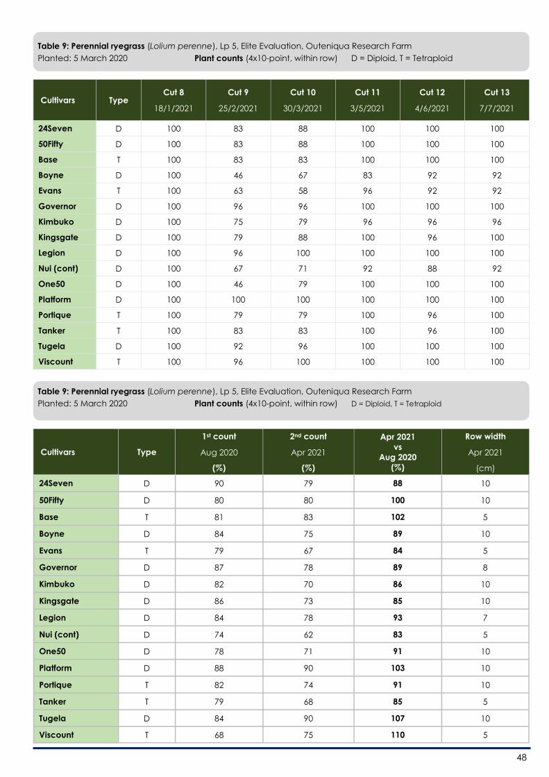
48
Table 9: Perennial ryegrass (Lolium perenne), Lp 5, Elite Evaluation, Outeniqua Research Farm
Planted: 5 March 2020 Plant counts (4x10-point, within row) D = Diploid, T = Tetraploid
Cultivars Type Cut 8
18/1/2021
Cut 9
25/2/2021
Cut 10
30/3/2021
Cut 11
3/5/2021
Cut 12
4/6/2021
Cut 13
7/7/2021
24Seven D 100 83 88 100 100 100
50Fifty D 100 83 88 100 100 100
Base T 100 83 83 100 100 100
Boyne D 100 46 67 83 92 92
Evans T 100 63 58 96 92 92
Governor D 100 96 96 100 100 100
Kimbuko D 100 75 79 96 96 96
Kingsgate D 100 79 88 100 96 100
Legion D 100 96 100 100 100 100
Nui (cont) D 100 67 71 92 88 92
One50 D 100 46 79 100 100 100
Platform D 100 100 100 100 100 100
Portique T 100 79 79 100 96 100
Tanker T 100 83 83 100 96 100
Tugela D 100 92 96 100 100 100
Viscount T 100 96 100 100 100 100
Table 9: Perennial ryegrass (Lolium perenne), Lp 5, Elite Evaluation, Outeniqua Research Farm
Planted: 5 March 2020 Plant counts (4x10-point, within row) D = Diploid, T = Tetraploid
Cultivars Type
1st count
Aug 2020
(%)
2nd count
Apr 2021
(%)
Apr 2021
vs
Aug 2020
(%)
Row width
Apr 2021
(cm)
24Seven D 90 79 88 10
50Fifty D 80 80 100 10
Base T 81 83 102 5
Boyne D 84 75 89 10
Evans T 79 67 84 5
Governor D 87 78 89 8
Kimbuko D 82 70 86 10
Kingsgate D 86 73 85 10
Legion D 84 78 93 7
Nui (cont) D 74 62 83 5
One50 D 78 71 91 10
Platform D 88 90 103 10
Portique T 82 74 91 10
Tanker T 79 68 85 5
Tugela D 84 90 107 10
Viscount T 68 75 110 5

49
Leaf emergence rate
Table 10: Perennial ryegrass (Lolium perenne), Lp 5, Elite Evaluation, Outeniqua Research Farm
Planted: 5 March 2020 No. of days per leaf and projected harvest rotation based on 3-leaf stage
Parameter
5 Mar
to
18 May
2020
18 May
to
24 Jun
2020
24 Jun
to
3 Aug
2020
3 Aug
to
16 Sep 2020
16 Sep
to
21 Oct
2020
21 Oct
to
25 Nov
2020
25 Nov
to
22 Dec
2020
No. of days 13.1 13.5 16 13.5 11.7 11.7 12
Projected time to 3-
leaf 39 41 48 41 35 35 36
2.75-leaf
Shortest cycle 36 37 44 37 32 32 33
Parameter
22 Dec
2020
to
18 Jan
2021
18 Jan
to
25 Feb
2021
25 Feb
to
30 Mar
2021
30 Mar
to
3 May 2021
3 May
to
4 Jun 2021
4 Jun
to
7 Jul 2021
No. of days 12 9.8 10.2 10 11.6 12
Projected time to 3-
leaf 36 29 31 30 35 36
2.75-leaf
Shortest cycle 33 27 28 28 32 33
Leaf emergence rate depends on leaf growth rate
since leaves emerge consecutively, one after the
other once the previous leaf is fully extended.
Growth rate is mainly dependent on temperature
and soil moisture. If soil moisture is sufficient, then the
growth rate is mainly a function of temperature.
Defoliation or harvest at the 3-leaf stage is optimal
for the plant (carbohydrate reserves, root and tiller
growth) and optimal for production since the first
leaf dies once the fourth leaf emerges and yield
reaches a plateau after the third leaf. The plants
can at the earliest be defoliated at the 2.75-leaf
stage when necessary.
Summary
(trial results for first 15 months; the trial is continuing)
Total yield for the first year (Year 1)
Highest yielding cultivar: Viscount
Similar to the highest yielding: Platform,
Governor, 50Fifty, Base, Legion, Nui, Tanker,
One50
Total yield 15 months (incl. second autumn)
Highest yielding cultivar: Viscount
Similar yield: Platform, Governor, Legion, 50Fifty,
Base
This shows which cultivars continued strongly beyond
the summer.
Establishment and autumn 2020
Only two cultivars were significantly slower than
the rest as reflected in the autumn yield (Evans,
Portique). All other cultivars had a similar yield.
Winter yield 2020
Highest yielding: Platform, Legion
Similar yield: One50, Base, Nui
Spring 2020
As expected in spring, most cultivars produce
well and is the season of least concern.
Summer yield 2020/21
Highest yielding: Viscount
Similar yield: Governor, Base, 50Fifty
Second autumn (2021)
Highest yielding: Legion, Governor, Viscount,
Platform
Similar yield: 50Fifty, Tugela, 24Seven, Base,
Kingsgate
Lowest rust incidence (mainly October to February
but some cultivars September to May)
17% or less throughout:
Kimbuko, Governor, Legion
33% or less
Platform, Viscount

50
Reproductive tillers/bolting
No bolting: Kimbuko, Portique
Highest bolting incidence: Evans, Tanker,
Viscount
Followed by: Base, Kingsgate, Nui
Table 7 also shows the length of the flowering
window.
Low bolting and relatively short flowering
window: Boyne, Legion, Platform
Sward density after the first summer Feb 2021: lowest
values recorded in February with density increasing
again as conditions become more favourable.
100%: Platform
90-100%: Governor, Legion, Viscount, Tugela
80 – 89% : 24Seven, 50Fifty, Base, Tanker
75 – 79%: Kimbuko, Kingsgate, Portique
Plant counts comparing April 2021 to August 2020
using the 10-point/m x4 method :
Increased count (increased sward density):
Viscount, Tugela, Platform, Base
Unchanged: 50Fifty
References:
Cabrera Estrada JI, Delagarde R, Faverdin RP, Peyraud JL.
2004. Dry matter intake and eating rate of grass by
dairy cows is restricted by internal, but not external
water. Animal Feed Science and Technology 114:
59- 74.
Chapman DF. 2016. Using Ecophysiology to Improve Farm
Efficiency: Application in Temperate Dairy Grazing
Systems. In: Forage Plant Ecophysiology (ed
Matthews C). Agriculture 6, 17: 122 – 140.
Clarke RG and Eagling DR. 1994. Effects of pathogens on
perennial pasture grasses. New Zealand Journal of
Agricultural Research, 37: 319-327
John A and Ulyatt MJ. 1987. Importance of dry matter
content to voluntary intake of fresh grass forages.
Proceedings of the New Zealand Society of Animal
Production 47: 13 – 16.
Leaver JD 1985. Milk production from grazed temperate
grassland. Journal of Dairy Research 52: 313-344
Minson DJ. 1990. Forages in ruminant nutrition. Animal
feeding and nutrition. A Series of Monographs and
Treatises (Cunha TJ, Ed.)
Potter LR. 2007. Effect of crown rust on regrowth,
competitive ability and nutritional quality of
perennial and Italian ryegrasses. Plant Pathology
36:455 - 461
Verite R and Journet M. 1970. Effect of the Water Content
of Grass and Dehydration at Low Temperature
upon Its Feeding Value for Dairy Cows. Annales de
Zootechnie, 19, 255-268.

51
Italian and hybrid ryegrass cultivar evaluation results
for 2020/21
Sigrun Ammann*, Dalena Lombard, Lethu Zulu
Western Cape Department of Agriculture, Research and Technology Development, Directorate Plant
Sciences, Outeniqua Research Farm, P.O. Box 24, George 6530
Corresponding author: [email protected]
Introduction
The Italian and hybrid ryegrass (Lolium multiflorum
and L. hybridum) elite cultivar evaluation trial
2020/21 was planted on 4 March 2020 at the
Outeniqua Research Farm. The aim of the trial is to
evaluate the recent Italian and hybrid ryegrass
cultivars being used for intensive dairy pastures or
ones that are about to enter the market. This trial
provides local data to assist farmers with choosing
cultivars best suited to the region and to their
specific use of pastures. Preferably the cultivars
evaluated in this trial should be ones that persist for
at least a 12-month period, preferably 15 months.
There is however also a use for the shorter duration
cultivars in combination with other species or
cultivars to fill certain gaps. Since most ryegrass
cultivars are imported, this data provides insight into
the genetic potential and adaption for the southern
Cape coastal region. This data is specific for 2020/21
but the best cultivars are evaluated in successive
trials. For previous data refer to the Outeniqua
Information Day booklets for 2018, 2019 and 2020
which will give an indication of how cultivars
perform in different years of establishment.
Cultivars evaluated
The trial consists of 20 cultivars of which 18 are Italian
and two are hybrid ryegrass. Of the Italian cultivars
14 are diploid and four are tetraploid, while the
hybrid cultivars are both tetraploid.
Italian diploid: AgriBoost, Belluci, Bond,
Davinci, Fox, Icon, Jackpot, Knight, Podium,
Sukari, SupremeQ, Surge, Tabu+, Yolande
Italian tetraploid: Barmultra II, Elvis, Firkin,
Impact (synonym Udine),
Hybrid tetraploid: Green Spirit, Shogun
Parameters reported in this article
Total DM yield
Seasonal DM yield
DM content
Flowering behaviour (autumn and spring)
Persistence / sward density
The diploids were sown at 25 kg/ha while the
tetraploids were sown at 30kg/ha. The evaluation
was done in small plot trials cut with a reciprocating
mower at 5cm where material from the entire net
plot was weighed and sampled. The trials were top-
dressed with nitrogen fertilizer after each harvest,
and potassium fertilizer when necessary to account
for nutrient removal.
The harvest cycle is determined according to
physiological stage being 3-leaf or in spring canopy
closure. As the first cultivars reach these stages, the
trial is harvested. Since leaf emergence rate is
mainly driven by temperature as well as radiation
intensity, water and nutrient availability (Chapman
2016), most cultivars reach the 3-leaf stage at a
similar time.
Total yield (Table 1) is important, especially on farms
that have the means to conserve the surplus as

52
silage for later use. The establishment and input
costs are also similar regardless of yield, hence the
importance of choosing the cultivars with the best
yield.
Seasonal yield data (Table 1) is of value for
optimising fodder flow requirements especially for
the more challenging seasons which are generally
winter and summer as well as autumn. The question
is whether there are cultivars with both good winter
and summer yield. Alternatively it is advisable to
plant paddocks to different cultivars to take
advantage of different seasonal yield distributions
and also to spread risk. A high yielding spring cultivar
can for instance be considered for silage making of
surplus production. Other consideration are for
mixed pastures and how the seasonal yield can best
be matched with the yield of the other species in
the mixture.
Individual harvest yields and growth rates are given
in Table 3 and 4.
Dry matter (DM) content (Table 5) is a consideration
especially early in the season when the DM content
is generally low, since DM content in ryegrass can
negatively influence voluntary intake if it is very low
(Cabrera Estrada et al 2004, John & Ulyatt 1987,
Leaver 1985, Minson 1990. The work by Vértité &
Journet 1970 is also widely referenced where they
investigated reduced intake with decreasing DM
content. In mixtures with other species that have a
very low DM content tis can be taken into account.
Leaf rust incidence (Table 6) refers mainly to crown
rust (Puccinia coronata). According to Clarke &
Eagling (1994) and Webb et al (2019) crown rust
causes yield loss as well as negative effects on root
weight and rooting depth, tiller numbers and leaf
area or photosynthetic area. Potter (2007) reported
not only reduced yield but also reduced water-
soluble carbohydrates and reduced digestibility.
Plummer et al (1990) also refers to reduced tiller
density and increased tiller death. Carr 1975 report
rust to be a water soluble carbohydrate (WSC) sink
that reduces growth and forage quality.
Additionally he estimates that 10% leaf rust infection
could cause up to 50% decline in WSC
concentration. Hence there are advantages to
cultivars which are resistant or have a low incidence
only.
Rust can be more severe under nutrient deficiency
conditions or if growth cycles are allowed to
continue beyond the 3-leaf stage. Increased dead
leaf matter may also increase facial eczema
(McKenzie 1971).
Sward density (Table 7) gives an indication of
persistence especially in the summer months. The
cultivars that retain good sward density or plant
population throughout the summer are desirable.
Italian ryegrass can also be used for spring-planting.
However only the cultivars with a low flowering
incidence are suitable for spring-planting since early
bolting will negatively affect such a planting. For
these results refer to the 2020 booklet. The next
evaluation is planned for spring 2021.
Flowering behaviour (Table 8) is important since it
results in a higher stem component which implies a
higher fibre content and thus lower nutritive value.
The percentage of the sward that is reproductive
varies significantly between cultivars as does the
duration of reproductive tillers in the sward. Cultivars
that do have a high bolting percentage could for
instance be used for paddocks that will be cut for
silage although it would also affect the silage quality
as opposed to cutting a non-reproductive sward
that is leafy. In mixtures with species that are very
competitive and tall growing in summer it might be
an advantage to have a ryegrass component with
a higher bolting percentage as that results in taller
plants to compete with the other tall components
for example chicory or lucerne.
The majority of Italian ryegrass cultivars that are
available have the ability to produce new
vegetative daughter tillers after the flowering phase.
These are then referred to as Italian ryegrasses with
a long growth duration. There are also cultivars that
do not produce vegetative tillers after the flowering
phase and thus end after the bolting phase. In the
current trial there are two such cultivars, AgriBoost
and SupremeQ.
Plant counts (Table 9) were done twice, in June 2020
after successful establishment of the trial and again
in April 2021 representing recovery after the summer
months. The 10-point method was used for these
counts. It consists of 10 pins on a wooden bar that
are spaced 10cm apart. The bar is placed randomly
within four rows within the plot and the number of
strikes are counted i.e. how many spikes are in
contact with a plant. Thus the number of strikes out

53
of 40 are then used to calculate a percentage. The
table gives the percentage decrease in plant over
the 10 month period giving an indication of
persistence into the second autumn.
Leaf emergence rate (Table 10) depends on leaf
growth rate since leaves emerge consecutively, one
after the other once the previous leaf is fully
extended. Growth rate is mainly dependent on
temperature and soil moisture. If soil moisture is
sufficient, then the growth rate is mainly a function
of temperature. Defoliation or harvest at the 3-leaf
stage is optimal for the plant (carbohydrate
reserves, root and tiller growth) and optimal for
production since the first leaf dies once the fourth
leaf emerges and yield reaches a plateau after the
third leaf. The plants can at the earliest be
defoliated at the 2.75-leaf stage when necessary. In
spring canopy closure should be used as primary
criterion to decide on the optimal defoliation time
since limiting light penetration into the base of the
sward can reduce daughter tiller initiation.

54
Tab
le 1
: It
alia
n a
nd
hy
bri
d r
ye
gra
ss (
Loliu
m m
ultiflo
rum
& L
. h
yb
rid
um
), L
m 1
0, Elit
e E
va
lua
tio
n, O
ute
niq
ua
Re
sea
rch
Fa
rm
Pla
nte
d: 4
Ma
rch
202
0
Se
aso
na
l Y
ield
(t
DM
/ha
) D
= D
iplo
id, T
= T
etr
ap
loid
, I =
Ita
lian
, H
= H
yb
rid
Sh
ad
ed
= h
igh
est
yie
ldin
g,
BO
LD =
sim
ilar
to h
igh
est
. N
ote
: tr
ea
tme
nts
with
th
e s
am
e le
tte
r a
re s
imila
r i.e
. n
ot
sig
nific
an
tly
diffe
ren
t
NS =
no
n-s
ign
ific
an
t
C
ultiv
ars
Ty
pe
A
utu
mn
2020
R
an
k
W
inte
r 20
20
R
an
k
Sp
rin
g
20
20
R
an
k
Su
mm
er
20
20
/21
R
an
k
A
utu
mn
2021
R
an
k
Tota
l Y
ea
r 1
Ra
nk
To
tal
15 m
on
ths
R
an
k
Ag
riB
oo
st
DI
2.5
1
1
2.3
0 c
de
15
3
.28
h
19
-
-
8
.07
h
20
8
.07
k
20
Ba
rmu
ltra
II
TI
2.3
6
4
2.5
6 a
bc
de
10
5
.70
a
1
2.5
6 d
efg
9
3.3
2 a
bc
3
13.2
ab
c
3
16.5
ab
c
3
Be
llu
ci
DI
2.3
4
6
2.7
1 a
bc
d
7
5.6
2 a
2
3
.52
ab
2
3.7
4 a
1
14.2
a
1
17.9
a
1
Bo
nd
D
I 2
.16
8
2.6
4 a
bc
de
8
5.2
4 a
bc
d
6
2.9
0 a
bc
de
5
3.0
2 b
cd
ef
9
12.9
ab
cd
4
16
.0 b
cd
5
Da
vin
ci
DI
1.7
1
19
2
.15
e
19
5
.37
ab
c
4
2.7
6 c
de
f 7
3.2
9 a
bc
d
4
12
.0 b
cd
e
10
1
5.3
bc
de
f 8
Elv
is
TI
2.1
6
9
2.2
3 d
e
18
5
.27
ab
cd
5
2.5
3 d
efg
h
10
3
.02
bc
de
f 1
0
12
.2 b
cd
9
15
.2 b
cd
ef
10
Fir
kin
TI
1
.62
2
0
2.2
5 d
e
16
4
.68
efg
1
3
1.8
6 g
hi
16
2
.60
efg
1
4
10
.4 e
fg
17
1
3.0
gh
i 1
6
Fo
x
DI
1.9
4
16
2.4
8 a
bc
de
12
5
.47
ab
3
3.6
0 a
1
3
.22
bc
d
6
13.5
ab
2
16.7
ab
2
Gre
en
Sp
irit
T
Mix
2
.04
1
3
2.5
5 a
bc
de
11
5
.16
a
bc
de
7
2.7
2 c
de
f 8
3.2
7 a
bc
d
5
12
.5 b
cd
8
15
.7 b
cd
e
6
Ico
n
DI
2.0
0
15
2
.13
e
20
4
.74
de
fg
12
2
.78
bc
de
f 6
3
.19
bc
d
7
11
.6 c
de
f 1
4
14
.9 c
def
12
Imp
ac
t/
Ud
ine
TI
1
.91
1
7
2.9
4 a
1
3
.23
h
20
1
.29
ij
18
2
.53
fg
15
9
.33
gh
19
1
1.9
ij
18
Ja
ck
po
t D
I 2
.35
5
2.8
1 a
bc
4
4.2
7 g
1
7
2.3
9 e
fgh
13
1
.97
h
17
1
1.8
cd
e
13
1
3.8
fg
h
15
Kn
igh
t D
I 2
.03
1
4
2.8
0 a
bc
5
4.2
5 g
1
8
2.5
1 d
efg
h
12
2
.50
g
16
1
1.6
de
f 1
5
14
.1 e
fgh
14
Po
diu
m
DI
2.1
0
11
2
.31
cd
e
14
4
.87
cd
ef
11
2
.52
de
fgh
11
3
.08
bc
de
8
11
.8 c
de
12
1
4.9
cd
ef
11
Sh
og
un
TH
1
.71
1
8
2.8
8 a
b
3
4.8
9 c
def
10
3
.39
ab
c
3
2.8
5 c
de
fg
11
12.9
ab
cd
5
15
.7 b
cd
e
7
Su
ka
ri
DI
2.4
5
2
2.9
3 a
2
5
.01
bc
de
9
2.1
1 f
gh
15
2
.79
de
fg
12
1
2.5
bc
d
7
15
.3 b
cd
ef
9
Su
pre
me
Q
DI
2.1
5
10
2.7
9 a
bc
6
4.3
9 f
g
15
0
.82
j 1
9
-
10
.1 f
g
18
1
0.1
j 1
9
Su
rge
D
I 2
.22
7
2
.23
de
17
4
.29
g
16
1
.79
hi
17
1
.88
h
18
1
0.5
efg
1
6
12
.4 h
i 1
7
Tab
u +
D
I 2
.38
3
2.5
7 a
bc
de
9
4.6
5 e
fg
14
2
.22
efg
h
14
2
.64
efg
1
3
11
.8 c
de
11
1
4.4
de
fg
13
Yo
lan
de
D
I 2
.08
1
2
2.3
7 b
cd
e
13
5
.05
bc
de
8
3.1
5 a
bc
d
4
3.4
0 a
b
2
12.6
ab
cd
6
16
.0 b
cd
4
LSD
(0
.05
)
NS
0.5
3
0
.54
0.7
5
0
.50
1.5
8
1
.78
CV
%
3
1.0
12
.6
6
.91
18
.0
1
0.3
8.1
0
7
.49

55
Tab
le 2
: It
alia
n a
nd
hy
bri
d r
ye
gra
ss (
Loliu
m m
ultiflo
rum
& L
. h
yb
rid
um
), L
m 1
0, Elit
e E
va
lua
tio
n, O
ute
niq
ua
Re
sea
rch
Fa
rm
Pla
nte
d: 4
Ma
rch
202
0
M
ea
n s
ea
son
al g
row
th r
ate
(kg
DM
/ha
/da
y)
D =
Dip
loid
, T
= T
etr
ap
loid
, I =
Ita
lian
, H
= H
yb
rid
Cu
ltiv
ars
Ty
pe
Au
tum
n
2020
Ra
nk
Win
ter
20
20
Ra
nk
Sp
rin
g
20
20
Ra
nk
Su
mm
er
2020/2
1
Ra
nk
Au
tum
n
2021
Ra
nk
Ag
riB
oo
st
DI
27
.3
1
25
.0 c
de
15
36
.0
h
18
-
-
Ba
rmu
ltra
II
TI
25
.7
4
27
.9 a
bc
de
10
62
.6 a
1
2
8.5
de
fg
9
36.1
ab
c
3
Be
llu
ci
DI
25
.4
6
29
.4 a
bc
d
7
61
.7 a
2
39.2
ab
2
40.6
a
1
Bo
nd
D
I 2
3.5
8
2
8.7
ab
cd
e
8
57
.6 a
bc
d
6
32.3
ab
cd
5
32
.8 b
cd
ef
9
Da
vin
ci
DI
18
.6
18
23
.3 e
1
9
59
.1 a
bc
4
30
.7 c
de
f 7
35.7
ab
c
4
Elv
is
TI
23
.5
9
24
.3 d
e
18
57
.9 a
bc
d
5
28
.1 d
efg
h
10
32
.8 b
cd
ef
10
Fir
kin
TI
1
7.6
2
0
24
.4 d
e
16
51
.5 e
fg
13
20
.7 g
hi
16
28
.3 e
fg
14
Fox
D
I 2
1.1
1
6
27.0
ab
cd
e
12
60.1
ab
3
40.0
a
1
35
.1 b
cd
6
Gre
en
Sp
irit
T M
ix
22
.2
13
27
.7 a
bc
de
11
56
.7 a
bc
de
7
30
.2 c
de
f 8
35.5
ab
cd
5
Ico
n
DI
21
.8
15
23
.2 e
2
0
52
.1 d
efg
1
2
30
.9 b
cd
ef
6
34
.6 b
cd
7
Imp
ac
t/U
din
e
TI
20
.8
17
31
.9 a
1
3
5.4
h
20
14
.4 i
18
27
.5 f
g
15
Ja
ck
po
t D
I 2
5.5
5
3
0.5
ab
c
4
47
.0 g
1
7
26
.5 e
fgh
13
21
.3 h
1
7
Kn
igh
t D
I 2
2.1
1
4
30
.4 a
bc
5
46
.8 g
1
8
27
.9 d
efg
h
12
27
.1 g
1
6
Po
diu
m
DI
22
.8
11
25
.2 c
de
14
53
.6 c
de
f 1
1
28
.0 d
efg
h
11
33
.4 b
cd
e
8
Sh
og
un
TH
1
8.5
1
8
31
.3 a
b
3
53
.7 c
de
f 1
0
37.7
ab
c
3
31
.0 c
de
fg
11
Su
ka
ri
DI
26
.8
2
31
.8 a
2
5
5.0
bc
de
9
23
.4 f
gh
15
30
.3 d
efg
1
2
Su
pre
me
Q
DI
23
.4
10
30
.4 a
bc
6
48
.2 f
g
15
-
-
Su
rge
D
I 2
4.1
7
2
4.3
de
17
47
.1 g
1
6
19
.9 h
i 1
7
20
.5 h
1
8
Tab
u +
D
I 2
5.8
3
2
8.0
ab
cd
e
9
51
.0 e
fg
14
24
.7 e
fgh
14
28
.7 e
fg
13
Yo
lan
de
D
I 2
2.6
1
2
25
.7 b
cd
e
13
55
.5 b
cd
e
8
35.0
ab
cd
4
36.9
ab
2
LSD
(0
.05
)
NS
5
.74
5
.99
8
.45
5
.41
CV
%
3
1.0
12
.6
6
.91
1
7.7
10
.3
Sh
ad
ed
= h
igh
est
yie
ldin
g,
BO
LD =
sim
ilar
to h
igh
est
. N
ote
: tr
ea
tme
nts
with
th
e s
am
e le
tte
r a
re s
imila
r i.e
. n
ot
sig
nific
an
tly
diffe
ren
t
NS =
no
n-s
ign
ific
an
t
M
ore
de
taile
d g
row
th r
ate
s a
re g
ive
n in
Ta
ble
4

56
Tab
le 3
: It
alia
n a
nd
hy
bri
d r
ye
gra
ss (
Loliu
m m
ultiflo
rum
& L
. h
yb
rid
um
), L
m 1
0, Elit
e E
va
lua
tio
n, O
ute
niq
ua
Re
sea
rch
Fa
rm
Pla
nte
d: 4
Ma
rch
202
0
Y
ield
(t
DM
/ha
) In
div
idu
al h
arv
est
s D
= D
iplo
id, T
= T
etr
ap
loid
, I =
Ita
lian
, H
= H
yb
rid
Cu
ltiv
ars
Ty
pe
Cu
t 1
12
/5/2
02
0
Cu
t 2
12
/6/2
02
0
Cu
t 3
29
/7/2
02
0
Cu
t 4
8/9
/202
0
Cu
t 5
7/1
0/2
02
0
Cu
t 6
2/1
1/2
02
0
Cu
t 7
26
/11
/20
20
Ag
riB
oo
st
DI
1.9
2
0.9
7 b
c
0.7
7 c
de
1.4
3 b
cd
e
1.5
2 g
0
.77
i 0
.72
i
Ba
rmu
ltra
II
TI
1.7
0
1.0
8 a
bc
0.8
7 b
cd
e
1.5
9 a
bc
de
2.1
9 a
b
1.9
5 a
b
1.2
5 a
bc
Be
llu
ci
DI
1.6
2
1.1
8 a
bc
1.1
2 a
b
1.4
1 b
cd
e
2.1
1 a
bc
2.0
3 a
1.2
1 a
bc
Bo
nd
D
I 1
.41
1.2
2 a
b
0.9
1 a
bc
de
1.5
7 a
bc
de
2.0
2 a
bc
d
1.7
3 b
cd
e
1.1
8 a
bc
d
Da
vin
ci
DI
1.1
3
0.9
4 c
0
.67
e
1.3
9 c
de
2.1
8 a
b
1.8
3 a
bc
1.0
9 c
de
f
Elv
is
TI
1.4
9
1.1
0 a
bc
0.8
4 b
cd
e
1.2
0 e
1
.82
de
f 1.8
8 a
b
1.3
4 a
Fir
kin
TI
1
.04
0.9
5 c
0
.73
de
1.4
4 b
cd
e
2.0
0 a
bc
d
1.5
1 e
fg
0.8
9 g
hi
Fox
D
I 1
.26
1.1
1 a
bc
0.8
4 b
cd
e
1.5
1 a
bc
de
2.2
7 a
1
.72
bc
de
1.1
9 a
bc
d
Gre
en
Sp
irit
T M
ix
1.3
7
1.0
9 a
bc
1.0
4 a
bc
1.3
4 c
de
2.0
4 a
bc
d
1.7
2 b
cd
e
1.1
4 a
bc
de
Ico
n
DI
1.3
1
1.1
3 a
bc
0.7
2 d
e
1.2
1 e
1
.94
bc
d
1.6
1 c
de
f 0
.96
efg
h
Imp
ac
t/U
din
e
TI
1.2
3
1.1
0 a
bc
0.9
8 a
bc
d
1.9
0 a
1
.16
h
0.8
4 i
0.8
6 h
i
Ja
ck
po
t D
I 1
.64
1.1
6 a
bc
0.9
9 a
bc
d
1.6
9 a
bc
1.8
0 d
ef
1.1
9 h
0
.95
efg
h
Kn
igh
t D
I 1
.36
1.1
0 a
bc
1.0
1 a
bc
d
1.6
9 a
bc
1.6
5 e
fg
1.2
0 h
1
.07
cd
efg
Po
diu
m
DI
1.4
1
1.1
3 a
bc
0.7
3 d
e
1.4
3 b
cd
e
2.0
5 a
bc
d
1.5
9 d
ef
0.9
6 e
fgh
Sh
og
un
TH
1
.00
1.1
4 a
bc
1.1
9 a
1
.55
ab
cd
e
1.8
0 d
ef
1.4
7 f
g
1.3
1 a
b
Su
ka
ri
DI
1.7
1
1.2
3 a
0
.96
ab
cd
e
1.8
6 a
b
2.1
8 a
b
1.3
4 g
h
1.1
2 b
cd
ef
Su
pre
me
Q
DI
1.4
3
1.1
7 a
bc
0.9
9 a
bc
d
1.6
8 a
bc
d
1.8
9 c
de
1.1
9 h
0
.97
efg
h
Su
rge
D
I 1
.55
1.0
8 a
bc
0.8
1 c
de
1.2
4 d
e
1.6
1 f
g
1.5
1 e
fg
0.9
2 f
gh
Tab
u +
D
I 1
.67
1.1
6 a
bc
1.0
1 a
bc
d
1.3
8 c
de
1.9
7 b
cd
1.4
3 g
h
0.9
9 d
efg
h
Yo
lan
de
D
I 1
.42
1.0
8 a
bc
0.9
2 a
bc
de
1.2
8 c
de
1.8
7 c
de
f 1.8
2 a
bc
d
1.1
1 b
cd
ef
LSD
(0
.05
)
NS
0.2
5
0.2
9
0.4
5
0.2
8
0.2
4
0.2
0
CV
%
4
1.9
1
3.7
1
9.7
1
8.2
8
.85
9.7
0
11
.7
Sh
ad
ed
= h
igh
est
yie
ldin
g,
BO
LD =
sim
ilar
to h
igh
est
. N
ote
: tr
ea
tme
nts
with
th
e s
am
e le
tte
r a
re s
imila
r i.e
. n
ot
sig
nific
an
tly
diffe
ren
t.

57
Tab
le 3
: It
alia
n a
nd
hy
bri
d r
ye
gra
ss (
Loliu
m m
ultiflo
rum
& L
. h
yb
rid
um
), L
m 1
0, Elit
e E
va
lua
tio
n, O
ute
niq
ua
Re
sea
rch
Fa
rm
Pla
nte
d: 4
Ma
rch
202
0
Y
ield
(t
DM
/ha
) In
div
idu
al h
arv
est
s D
= D
iplo
id, T
= T
etr
ap
loid
, I =
Ita
lian
, H
= H
yb
rid
Sh
ad
ed
= h
igh
est
yie
ldin
g,
BO
LD =
sim
ilar
to h
igh
est
. N
ote
: tr
ea
tme
nts
with
th
e s
am
e le
tte
r a
re s
imila
r i.e
. n
ot
sig
nific
an
tly
diffe
ren
t.
* h
ea
t st
ress
co
nd
itio
ns
the
we
ek
be
fore
ha
rve
st
Cu
ltiv
ars
Ty
pe
C
ut
8
17
/12
/20
20
Cu
t 9
12
/1/2
02
1
Cu
t 1
0 *
10
/2/2
02
1
Cu
t 1
1
5/3
/202
1
Cu
t 12
7/4
/202
1
Cu
t 13
5/5
/202
1
Cu
t 14
7/6
/202
1
Ag
riB
oo
st
DI
- -
- -
- -
-
Ba
rmu
ltra
II
TI
1.1
1 a
bc
d
0.7
6 d
e
0.2
7 b
cd
e
0.5
5 a
bc
1.2
5 a
bc
d
1.1
9 b
cd
0.9
7 a
Be
llu
ci
DI
1.3
0 a
1
.08
ab
c
0.5
9 a
b
0.7
2 a
b
1.4
7 a
1.4
0 a
0.9
0 a
b
Bo
nd
D
I 1
.06
bc
d
0.9
6 a
bc
de
0.4
1 a
bc
d
0.6
2 a
b
1.1
0 b
cd
e
1.0
4 d
ef
0.9
5 a
Da
vin
ci
DI
0.9
6 c
de
0.9
2 b
cd
e
0.4
2 a
bc
d
0.5
9 a
b
1.2
7 a
bc
1.1
8 b
cd
0.9
0 a
b
Elv
is
TI
1.1
7 a
bc
0.8
1 c
de
0.2
5 c
de
0.3
9 a
bc
d
1.1
6 a
bc
de
1.0
9 c
de
0.8
8 a
bc
d
Fir
kin
TI
0
.96
cd
e
0.7
4 d
e
0.0
9 e
0
.09
cd
0.9
0 d
ef
1.1
0 c
d
0.7
4 d
efg
Fo
x
DI
1.1
0 a
bc
d
1.2
4 a
0
.59
a
0.8
6 a
1.2
8 a
bc
1.1
0 c
d
0.8
4 a
bc
de
Gre
en
Sp
irit
T M
ix
1.1
4 a
bc
d
0.7
8 d
e
0.3
6 a
bc
de
0.5
5 a
bc
1.2
0 a
bc
d
1.2
4 a
bc
0.9
0 a
bc
Ico
n
DI
1.0
7 a
bc
d
1.0
0 a
bc
d
0.3
6 a
bc
de
0.4
7 a
bc
d
1.3
6 a
b
1.1
7 b
cd
0.7
2 e
fg
Imp
ac
t/U
din
e
TI
0.9
3 d
e
0.1
5 f
0.0
8 e
0
.26
bc
d
0.8
3 e
f 1
.06
de
f 0
.76
bc
de
fg
Ja
ck
po
t D
I 1
.03
bc
de
0.9
2 b
cd
e
0.1
8 d
e
0.5
1 a
bc
d
0.5
5 f
0.9
0 f
g
0.5
6 h
Kn
igh
t D
I 0
.95
cd
e
0.9
7 a
bc
de
0.2
8 a
bc
de
0.6
6 a
b
0.9
9 c
de
0.9
2 e
fg
0.6
4 g
h
Po
diu
m
DI
0.9
9 b
cd
e
0.8
4 c
de
0.3
6 a
bc
de
0.4
2 a
bc
d
1.2
2 a
bc
d
1.1
4 b
cd
0.7
9 b
cd
ef
Sh
og
un
TH
1.2
2 a
b
1.1
6 a
b
0.5
4 a
bc
0.6
2 a
b
1.1
0 b
cd
e
1.0
3 d
ef
0.7
5 c
de
fg
Su
ka
ri
DI
0.9
2 d
e
0.8
3 c
de
0.1
7 d
e
0.3
8 a
bc
d
1.0
5 b
cd
e
1.1
0 c
d
0.7
5 d
efg
Su
pre
me
Q
DI
0.8
2 e
-
- -
- -
-
Su
rge
D
I 0
.81
e
0.8
0 c
de
0.1
5 d
e
0.0
6 d
0
.59
f
0.8
4 g
0
.55
h
Tab
u +
D
I 1.1
1 a
bc
d
0.7
1 e
0
.15
de
0.3
2 b
cd
1.0
2 b
cd
e
1.0
4 d
ef
0.6
5 f
gh
Yo
lan
de
D
I 1.2
1 a
b
1.0
3 a
bc
d
0.4
7 a
bc
d
0.5
6 a
bc
1.3
1 a
bc
1.2
9 a
b
0.8
6 a
bc
de
LSD
(0
.05
)
0.2
4
0.2
9
0.3
2
0.4
9
0.3
7
0.1
7
0.1
5
CV
%
1
3.6
2
0.5
6
1.5
5
5.6
2
0.4
9
.3
11
.4

58
Tab
le 4
Ita
lia
n a
nd
hy
bri
d r
ye
gra
ss (
Loliu
m m
ult
iflo
rum
& L
. h
yb
rid
um
), L
m 1
0, Elit
e E
va
lua
tio
n, O
ute
niq
ua
Re
sea
rch
Fa
rm
Pla
nte
d: 4
Ma
rch
202
0
G
row
th r
ate
s (k
g D
M/h
a/d
ay)
Ind
ivid
ua
l h
arv
est
s D
= D
iplo
id, T
= T
etr
ap
loid
, I =
Ita
lian
, H
= H
yb
rid
Sh
ad
ed
= h
igh
est
yie
ldin
g,
BO
LD =
sim
ilar
to h
igh
est
. N
ote
: tr
ea
tme
nts
with
th
e s
am
e le
tte
r a
re s
imila
r i.e
. n
ot
sig
nific
an
tly
diffe
ren
t.
Cu
ltiv
ars
Ty
pe
C
ut
1
12
/5/2
02
0
Cu
t 2
12
/6/2
02
0
Cu
t 3
29
/7/2
02
0
Cu
t 4
8/9
/202
0
Cu
t 5
7/1
0/2
02
0
Cu
t 6
2/1
1/2
02
0
Cu
t 7
26
/11
/20
20
Ag
riB
oo
st
DI
27
.8
31
.4 b
1
6.4
cd
e
35
.0 b
cd
e
52
.4 g
2
9.4
h
29
.8 i
Ba
rmu
ltra
II
TI
24
.7
34.7
ab
18
.5 b
cd
e
38.7
ab
cd
e
75.5
ab
74.9
ab
52.1
ab
c
Be
llu
ci
DI
23
.4
38
.0 a
b
23
.8 a
b
34
.4 b
cd
e
72.6
ab
c
77.9
a
50.5
ab
c
Bo
nd
D
I 2
0.5
3
9.5
a
19
.3 a
bc
de
38
.2 a
bc
de
69.5
ab
cd
66
.7 b
cd
49.2
ab
cd
Da
vin
ci
DI
16
.4
30
.4 b
1
4.2
e
33
.8 c
de
75.2
ab
70.5
ab
c
45
.5 b
cd
ef
Elv
is
TI
21
.6
35
.4 a
b
17
.9 b
cd
e
29
.2 e
6
2.9
de
f 72.2
ab
55.8
a
Fir
kin
TI
1
5.0
3
0.5
b
15
.4 d
e
35
.1 b
cd
e
69.0
ab
cd
58
.1 d
ef
37
.1 g
hi
Fox
D
I 1
8.2
35.8
ab
17
.9 b
cd
e
36.8
ab
cd
e
78.2
a
66
.2 b
cd
49.5
ab
cd
Gre
en
Sp
irit
T M
ix
20
.0
35
.2 a
b
22
.3 a
bc
32
.7 c
de
70.3
ab
cd
66
.1 b
cd
47.6
ab
cd
e
Ico
n
DI
19
.0
36
.5 a
b
15
.3 d
e
29
.5 e
6
6.7
bc
d
61
.8 c
de
40
.1 e
fgh
Imp
ac
t/U
din
e
TI
17
.9
35
.6 a
b
20
.9 a
bc
d
46
.3 a
4
0.0
h
32
.1 h
3
5.7
hi
Ja
ck
po
t D
I 2
3.7
3
7.5
ab
21
.1 a
bc
d
41
.4 a
bc
62
.1 d
ef
45
.8 g
3
9.5
efg
h
Kn
igh
t D
I 1
9.7
3
5.5
ab
21
.5 a
bc
d
41
.2 a
bc
57
.1 e
fg
46
.3 g
4
4.4
cd
efg
Po
diu
m
DI
20
.5
36
.3 a
b
15
.6 d
e
34
.8 b
cd
e
70.7
ab
cd
61
.2 c
de
39
.8 e
fgh
Sh
og
un
TH
1
4.5
3
6.9
ab
25
.2 a
3
7.8
ab
cd
e
62
.2 d
ef
56
.8 e
f 54.5
ab
Su
ka
ri
DI
24
.8
39
.7 a
2
0.4
ab
cd
e
45
.3 a
b
75.3
ab
51
.5 f
g
46
.8 b
cd
ef
Su
pre
me
Q
DI
20
.7
37
.9 a
b
20
.9 a
bc
d
41
.1 a
bc
d
65
.3 c
de
45
.9 g
4
0.6
efg
h
Su
rge
D
I 2
2.5
3
5.0
ab
17
.2 c
de
30
.3 d
e
55
.6 f
g
58
.0 d
ef
38
.5 f
gh
Tab
u +
D
I 2
4.2
3
7.4
ab
21
.5 a
bc
d
33
.7 c
de
67
.7 b
cd
54
.8 e
fg
41
.1 d
efg
h
Yo
lan
de
D
I 2
0.5
3
5.0
ab
19
.5 a
bc
de
31
.3 c
de
64
.3 c
de
f 70.2
ab
c
46
.2 b
cd
ef
LSD
(0
.05
)
NS
8.0
9
6.2
6
10
.9
9.6
2
9.3
3
8.5
8
CV
%
4
1.9
1
3.7
1
9.7
1
8.2
8
.85
9.7
0
11
.7

59
Tab
le 4
Ita
lia
n a
nd
hy
bri
d r
ye
gra
ss (
Loliu
m m
ult
iflo
rum
& L
. h
yb
rid
um
), L
m 1
0, Elit
e E
va
lua
tio
n, O
ute
niq
ua
Re
sea
rch
Fa
rm
Pla
nte
d: 4
Ma
rch
202
0
G
row
th r
ate
s (k
g D
M/h
a/d
ay)
Ind
ivid
ua
l h
arv
est
s D
= D
iplo
id, T
= T
etr
ap
loid
, I =
Ita
lian
, H
= H
yb
rid
Sh
ad
ed
= h
igh
est
yie
ldin
g,
BO
LD =
sim
ilar
to h
igh
est
. N
ote
: tr
ea
tme
nts
with
th
e s
am
e le
tte
r a
re s
imila
r i.e
. n
ot
sig
nific
an
tly
diffe
ren
t.
* h
ea
t st
ress
co
nd
itio
ns
the
we
ek
be
fore
ha
rve
st
Cu
ltiv
ars
Ty
pe
C
ut
8
17
/12
/20
20
Cu
t 9
12
/1/2
02
1
Cu
t 1
0 *
10
/2/2
02
1
Cu
t 1
1
5/3
/202
1
Cu
t 12
7/4
/202
1
Cu
t 13
5/5
/202
1
Cu
t 14
7/6
/202
1
Ag
riB
oo
st
DI
- -
- -
- -
-
Ba
rmu
ltra
II
TI
52.9
ab
cd
29
.1 d
e
9.2
bc
d
23.8
ab
c
37.8
ab
cd
42
.7 b
cd
29.3
a
Be
llu
ci
DI
61.7
a
41
.4 a
bc
20
.3 a
3
1.3
ab
44.4
a
50.1
a
27.4
ab
Bo
nd
D
I 5
0.2
bc
d
37
.0 a
bc
de
14
.1 a
bc
26
.7 a
b
33
.2 b
cd
e
37
.2 d
ef
28.8
a
Da
vin
ci
DI
45
.7 c
de
35
.5 b
cd
e
14
.4 a
bc
25
.7 a
b
38.6
ab
c
42
.0 b
cd
27.3
ab
Elv
is
TI
55.8
ab
c
31
.0 c
de
8.7
bc
d
16
.5 a
bc
d
35.1
ab
cd
e
38
.8 c
de
26.6
ab
cd
Fir
kin
TI
4
5.8
cd
e
28
.5 d
e
2.9
d
4.1
cd
27
.3 d
ef
39
.2 c
d
22
.4 d
efg
Fox
D
I 52.3
ab
cd
47.7
a
20.3
a
37.2
a
38.8
ab
c
39
.3 c
d
25.4
ab
cd
e
Gre
en
Sp
irit
T M
ix
54.4
ab
cd
30
.0 c
de
12
.6 a
bc
d
24
.0 a
bc
36.5
ab
cd
44.3
ab
c
27.1
ab
c
Ico
n
DI
50.8
ab
cd
38
.6 a
bc
de
12
.2 a
bc
d
19
.8 a
bc
d
41.0
ab
41
.7 b
cd
21
.8 e
fg
Imp
ac
t/U
din
e
TI
44
.2 d
e
6.0
f
2.6
d
11
.2 b
cd
25
.2 e
f 3
7.9
de
f 2
3.0
bc
de
fg
Ja
ck
po
t D
I 4
8.9
bc
de
35
.2 b
cd
e
6.2
cd
22
.0 a
bc
d
16
.7 f
32
.0 g
f 1
7.1
h
Kn
igh
t D
I 4
5.3
cd
e
37
.1 a
bc
de
9.7
ab
cd
26
.4 a
b
29
.9 c
de
32
.8 e
fg
19
.4 g
h
Po
diu
m
DI
47
.0 b
cd
e
32
.4 c
de
12
.4 a
bc
d
18
.3 a
bc
d
37.0
ab
cd
40
.8 b
cd
24
.1 b
cd
ef
Sh
og
un
TH
57.9
ab
44
.7 a
b
18
.7 a
b
26
.1 a
b
33
.1 b
cd
e
37
.0 d
ef
22
.8 c
de
fg
Su
ka
ri
DI
43
.7 d
e
31
.8 c
de
5.8
cd
16
.2 a
bc
d
31
.7 b
cd
e
39
.3 c
d
22
.6 d
efg
Su
pre
me
Q
DI
38
.9 e
-
- -
- -
-
Su
rge
D
I 3
8.7
e
30
.7 c
de
5.2
cd
2.3
d
18
.0 f
30
.1 g
1
6.8
h
Tab
u +
D
I 52.9
ab
cd
27
.5 e
5
.1 c
d
13
.7 b
cd
30
.9 b
cd
e
37
.1 d
ef
19
.7 f
gh
Yo
lan
de
D
I 57.9
ab
40
.0 a
bc
d
16
.1 a
bc
24
.3 a
bc
39.5
ab
c
46.2
ab
26.1
ab
cd
e
LSD
(0
.05
)
11
.2
11
.6
11
.1
21
.4
11
.1
6.0
8
4.4
9
CV
%
1
3.6
2
0.2
6
1.3
5
7.2
2
0.3
9
.3
11
.4

60
Tab
le 5
Ita
lia
n a
nd
hy
bri
d r
ye
gra
ss (
Loliu
m m
ult
iflo
rum
& L
. h
yb
rid
um
), L
m 1
0, Elit
e E
va
lua
tio
n, O
ute
niq
ua
Re
sea
rch
Fa
rm
Pla
nte
d: 4
Ma
rch
202
0
D
ry m
att
er
co
nte
nt
(%)
Ind
ivid
ua
l h
arv
est
s D
= D
iplo
id, T
= T
etr
ap
loid
, I =
Ita
lian
, H
= H
yb
rid
Cu
ltiv
ars
Ty
pe
C
ut
1
12
/5/2
02
0
Cu
t 2
12
/6/2
02
0
Cu
t 3
29
/7/2
02
0
Cu
t 4
8/9
/202
0
Cu
t 5
7/1
0/2
02
0
Cu
t 6
2/1
1/2
02
0
Cu
t 7
26
/11
/20
20
Ag
riB
oo
st
DI
13
.1 b
cd
e
14
.5 b
cd
e
21
.0 a
b
20
.0 a
bc
17.6
ab
cd
20.9
ab
c
21.7
a
Ba
rmu
ltra
II
TI
13
.2 b
c
13
.7 d
e
18
.8 d
1
8.2
cd
ef
16
.8 c
d
16
.9 j
16
.1 i
Be
llu
ci
DI
11
.6 e
f 1
4.5
bc
de
19
.6 b
cd
20
.0 a
bc
17.5
ab
cd
18
.5 g
hi
17
.7 d
efg
Bo
nd
D
I 15.0
a
15
.1 b
cd
e
21
.2 a
b
19
.2 b
cd
e
18.0
ab
cd
18
.7 f
gh
i 1
7.7
efg
h
Da
vin
ci
DI
13.7
ab
16
.2 a
b
20
.8 a
bc
19
.5 a
bc
d
17.7
ab
cd
19
.6 c
de
fgh
18
.7 c
de
f
Elv
is
TI
12
.6 b
cd
ef
14
.3 b
cd
e
19
.9 b
cd
18
.9 b
cd
e
17
.3 b
cd
17
.5 ij
16
.5 h
i
Fir
kin
TI
1
1.6
de
f 1
3.2
e
19
.5 b
cd
18
.5 c
de
17
.1 b
cd
18
.1 h
ij 1
7.8
de
fg
Fox
D
I 1
2.8
bc
de
f 1
5.4
bc
d
20.6
ab
cd
19.7
ab
c
17.7
ab
cd
18
.6 g
hi
17
.6 f
gh
Gre
en
Sp
irit
T M
ix
11
.9 c
de
f 1
4.0
cd
e
18
.8 d
1
8.8
bc
de
17
.5 b
cd
16
.9 j
16
.9 g
hi
Ico
n
DI
13
.4 b
1
7.9
a
21
.1 a
b
20
.2 a
bc
17.7
ab
cd
19
.4 c
de
fgh
18
.0 d
efg
Imp
ac
t/U
din
e
TI
11
.5 f
13
.2 e
1
9.1
cd
16
.8 d
ef
16
.4 d
1
9.1
efg
h
18
.7 c
de
f
Ja
ck
po
t D
I 1
2.8
bc
de
f 1
4.3
bc
de
18
.8
d
18
.4 c
de
17
.0 c
d
20
.2 b
cd
ef
18
.6 c
de
f
Kn
igh
t D
I 1
3.2
bc
14
.1 c
de
19
.8 b
cd
16
.5 e
f 1
6.8
cd
19
.2 d
efg
h
18
.5 c
de
f
Po
diu
m
DI
13.6
ab
15
.7 b
c
22.0
a
22.0
a
19.1
a
20.5
ab
cd
e
18
.9 c
de
Sh
og
un
TH
1
3.1
bc
d
14
.7 b
cd
e
19
.0 c
d
15
.6 f
17.8
ab
cd
19
.6 c
de
fgh
17
.6 f
gh
Su
ka
ri
DI
14.0
ab
15
.8 b
c
22
.3 a
2
1.3
ab
18.7
ab
21.8
a
20.6
ab
Su
pre
me
Q
DI
13
.3 b
c
15
.7 b
c
21
.1 a
b
20
.1 a
bc
18.1
ab
c
21.5
ab
19
.6 b
c
Su
rge
D
I 1
2.5
bc
de
f 1
5.5
bc
d
19
.6 b
cd
19
.5 a
bc
d
17.6
ab
cd
20.7
ab
cd
19
.5 b
c
Tab
u +
D
I 1
2.5
bc
de
f 1
5.2
bc
d
19
.4 b
cd
19
.5 a
bc
d
17
.3 b
cd
19
.7 c
de
fg
19
.0 c
d
Yo
lan
de
D
I 1
3.1
bc
de
14
.4 b
cd
e
20
.7 a
bc
21
.9 a
18.3
ab
c
19
.4 c
de
fgh
18
.7 c
de
f
LSD
(0
.05
)
1.5
1
1.9
3
1.8
2
2.6
7
1.6
6
1.4
7
1.2
1
CV
%
7
.05
7.8
6
5.4
8
8.4
0
5.7
0
4.5
9
3.9
9
Sh
ad
ed
= a
bo
ve
18
%, B
OLD
= h
igh
est
DM
, B
OLD
Ita
lic
s =
sim
ilar
to t
he
hig
he
st.. N
ote
: tr
ea
tme
nts
with
th
e s
am
e le
tte
r a
re s
imila
r i.e
. n
ot
sig
nific
an
tly
diffe
ren
t.

61
Tab
le 5
Ita
lia
n a
nd
hy
bri
d r
ye
gra
ss (
Loliu
m m
ult
iflo
rum
& L
. h
yb
rid
um
), L
m 1
0, Elit
e E
va
lua
tio
n, O
ute
niq
ua
Re
sea
rch
Fa
rm
Pla
nte
d: 4
Ma
rch
202
0
D
ry m
att
er
co
nte
nt
(%)
Ind
ivid
ua
l h
arv
est
s D
= D
iplo
id, T
= T
etr
ap
loid
, I =
Ita
lian
, H
= H
yb
rid
Sh
ad
ed
= a
bo
ve
18
%, B
OLD
= h
igh
est
DM
, B
OLD
Ita
lic
s =
sim
ilar
to t
he
hig
he
st.. N
ote
: tr
ea
tme
nts
with
th
e s
am
e le
tte
r a
re s
imila
r i.e
. n
ot
sig
nific
an
tly
diffe
ren
t.
* h
ea
t st
ress
co
nd
itio
ns
the
we
ek
be
fore
ha
rve
st
Cu
ltiv
ars
Ty
pe
C
ut
8
17
/12
/20
20
Cu
t 9
12
/1/2
02
1
Cu
t 1
0 *
10
/2/2
02
1
Cu
t 1
1
5/3
/202
1
Cu
t 12
7/4
/202
1
Cu
t 13
5/5
/202
1
Cu
t 14
7/6
/202
1
Ag
riB
oo
st
DI
- -
- -
- -
-
Ba
rmu
ltra
II
TI
14
.7 i
16
.0 d
2
2.8
ab
18
.5 b
cd
13
.8 b
cd
e
10
.6 f
gh
i 1
4.6
ij
Be
llu
ci
DI
17
.3 c
de
fg
16
.1 d
2
3.3
ab
17
.3 c
d
13
.6 b
cd
e
11
.1 c
de
fg
15
.9 c
de
fg
Bo
nd
D
I 1
8.1
bc
de
18
.1 a
bc
25
.7 a
b
18
.0 a
bc
15
.1 b
c
10
.9 d
efg
h
16
.6 b
cd
Da
vin
ci
DI
17
.8 b
cd
ef
17
.7 a
bc
d
25
.6 a
b
18
.9 b
cd
15
.0 b
cd
12
.0 b
1
6.7
bc
Elv
is
TI
15
.3 h
i 1
6.7
bc
d
24
.5 a
b
18
.0 b
cd
13
.1 d
e
10
.2 i
14
.3 j
Fir
kin
TI
1
8.1
bc
de
17
.5 a
bc
d
24
.6 a
b
18
.2 b
cd
13
.8 b
cd
e
10
.5 h
i 1
5.2
gh
i
Fox
D
I 1
7.4
cd
efg
1
7.2
bc
d
21
.4 b
1
7.4
cd
14
.1 b
cd
e
11
.3 c
d
16
.4 b
cd
Gre
en
Sp
irit
T M
ix
16
.4 f
gh
16
.4 c
d
24
.4 a
b
18
.0 b
cd
12
.8 e
1
0.6
gh
i 1
5.1
hij
Ico
n
DI
16
.8 e
fgh
16
.7 b
cd
25
.5 a
b
18
.9 b
c
14
.0 b
cd
e
11
.3 c
de
16
.2 b
cd
ef
Imp
ac
t/U
din
e
TI
16
.2 g
hi
16
.4 c
d
23
.0 a
b
19
.0 b
c
13
.6 b
cd
e
10
.8 e
fgh
i 1
5.1
hij
Ja
ck
po
t D
I 1
7.1
de
fg
17
.5 a
bc
d
25
.1 a
b
16
.3 d
1
4.8
bc
d
11
.0 c
de
fgh
15
.3 g
hi
Kn
igh
t D
I 1
8.0
bc
de
18
.5 a
b
27
.8 a
b
17
.3 c
d
14
.9 b
cd
10
.8 e
fgh
i 1
5.9
de
fg
Po
diu
m
DI
18
.6 b
cd
17.6
ab
cd
23.9
ab
19.6
ab
c
14
.5 b
cd
e
12
.0 b
1
7.0
b
Sh
og
un
TH
1
7.4
cd
efg
1
6.1
d
22
.6 a
b
18
.4 b
cd
14
.8 b
cd
11
.2 c
de
f 1
5.4
fg
h
Su
ka
ri
DI
20.3
a
19
.1 a
2
6.6
ab
22
.0 a
1
5.4
b
13.0
a
18.7
a
Su
pre
me
Q
DI
19.1
ab
- -
- -
- -
Su
rge
D
I 1
8.3
bc
d
17
.5 a
bc
d
28
.0 a
2
0.4
ab
17.6
a
11
.1 c
de
fgh
16
.5 b
cd
Tab
u +
D
I 1
8.7
bc
18
.1 a
bc
27
.9 a
1
7.9
bc
d
14
.6 b
cd
e
11
.5 b
c
15
.6 e
fgh
Yo
lan
de
D
I 1
7.9
bc
de
17
.2 b
cd
25
.3 a
b
20
.2 a
b
13
.3 d
e
11
.3 c
de
16
.3 b
cd
e
LSD
(0
.05
)
1.5
3
1.8
0
6.4
2
2.6
1
1.8
8
0.5
9
0.8
2
CV
%
5
.28
6.2
4
15
.5
8.4
8
7.9
1
3.1
8
3.1
2

62
Tab
le 6
Ita
lia
n a
nd
hy
bri
d r
ye
gra
ss (
Loliu
m m
ult
iflo
rum
& L
. h
yb
rid
um
), L
m 1
0, Elit
e E
va
lua
tio
n, O
ute
niq
ua
Re
sea
rch
Fa
rm
Pla
nte
d: 4
Ma
rch
202
0
Le
af
rust
(%
) (r
atin
g b
ase
d)
Ind
ivid
ua
l h
arv
est
s D
= D
iplo
id, T
= T
etr
ap
loid
, I =
Ita
lian
, H
= H
yb
rid
Cu
ltiv
ars
Ty
pe
C
ut
1
12
/5/2
02
0
Cu
t 2
12
/6/2
02
0
Cu
t 3
29
/7/2
02
0
Cu
t 4
8/9
/202
0
Cu
t 5
7/1
0/2
02
0
Cu
t 6
2/1
1/2
02
0
Cu
t 7
26
/11
/20
20
Ag
riB
oo
st
DI
25
4
4
0
0
0
0
Ba
rmu
ltra
II
TI
25
1
2.5
3
3
8
0
0
0
Be
llu
ci
DI
21
0
0
0
0
0
0
Bo
nd
D
I 2
1
4
0
0
4
0
0
Da
vin
ci
DI
21
1
2.5
1
7
0
4
0
0
Elv
is
TI
25
2
9
46
4
8
0
0
Fir
kin
TI
1
7
21
5
8
0
17
0
0
Fo
x
DI
21
0
8
4
0
0
4
Gre
en
Sp
irit
T
Mix
2
1
8
33
4
8
0
0
Ico
n
DI
17
8
8
0
0
0
4
Imp
ac
t/U
din
e
TI
0
0
0
0
0
0
0
Ja
ck
po
t D
I 2
5
0
4
0
0
0
0
Kn
igh
t D
I 4
0
0
0
0
0
0
Po
diu
m
DI
4
4
17
0
0
0
0
Sh
og
un
TH
1
2.5
2
1
29
0
8
4
8
Su
ka
ri
DI
0
0
0
0
0
0
0
Su
pre
me
Q
DI
4
0
0
0
0
0
0
Su
rge
D
I 2
1
0
0
0
0
0
0
Tab
u +
D
I 1
2.5
4
4
0
0
0
0
Yo
lan
de
D
I 8
0
4
0
0
4
0

63
Tab
le 6
Ita
lia
n a
nd
hy
bri
d r
ye
gra
ss (
Loliu
m m
ult
iflo
rum
& L
. h
yb
rid
um
), L
m 1
0, Elit
e E
va
lua
tio
n, O
ute
niq
ua
Re
sea
rch
Fa
rm
Pla
nte
d: 4
Ma
rch
202
0
Le
af
rust
(%
) (r
atin
g b
ase
d)
Ind
ivid
ua
l h
arv
est
s D
= D
iplo
id, T
= T
etr
ap
loid
, I =
Ita
lian
, H
= H
yb
rid
Cu
ltiv
ars
Ty
pe
C
ut
8
17
/12
/20
20
Cu
t 9
12
/1/2
02
1
Cu
t 1
0 *
10
/2/2
02
1
Cu
t 1
1
5/3
/202
1
Cu
t 12
7/4
/202
1
Cu
t 13
5/5
/202
1
Cu
t 14
7/6
/202
1
Ag
riB
oo
st
DI
0
- -
- -
- -
Ba
rmu
ltra
II
TI
0
25
0
4
1
2.5
0
0
Be
llu
ci
DI
0
0
4
0
4
0
0
Bo
nd
D
I 8
8
0
0
8
0
0
Da
vin
ci
DI
0
12
.5
0
0
17
4
0
Elv
is
TI
0
25
8
4
3
3
4
0
Fir
kin
TI
4
2
5
17
4
2
9
8
0
Fo
x
DI
0
17
4
0
2
1
0
0
Gre
en
Sp
irit
T
Mix
0
4
4
0
1
2.5
4
0
Ico
n
DI
4
0
0
0
0
4
0
Imp
ac
t/U
din
e
TI
0
0
4
0
12
.5
0
0
Ja
ck
po
t D
I 4
8
0
0
0
0
0
Kn
igh
t D
I 4
8
4
4
0
0
0
Po
diu
m
DI
0
17
0
0
1
2.5
4
0
Sh
og
un
TH
1
2.5
2
5
12
.5
0
21
1
2.5
0
Su
ka
ri
DI
0
0
0
0
0
0
0
Su
pre
me
Q
DI
0
0
- -
- -
-
Su
rge
D
I 0
0
0
0
0
4
0
Tab
u +
D
I 0
2
1
4
0
8
4
0
Yo
lan
de
D
I 0
8
0
0
8
4
0
*
he
at
stre
ss c
on
ditio
ns
the
we
ek
be
fore
ha
rve
st

64
Tab
le 7
Ita
lia
n a
nd
hy
bri
d r
ye
gra
ss (
Loliu
m m
ult
iflo
rum
& L
. h
yb
rid
um
), L
m 1
0, Elit
e E
va
lua
tio
n, O
ute
niq
ua
Re
sea
rch
Fa
rm
Pla
nte
d: 4
Ma
rch
202
0
Sw
ard
de
nsi
ty (
%)
(ra
tin
g b
ase
d)I
nd
ivid
ua
l h
arv
est
s D
= D
iplo
id, T
= T
etr
ap
loid
, I =
Ita
lian
, H
= H
yb
rid
Cu
ltiv
ars
Ty
pe
C
ut
1
12
/5/2
02
0
Cu
t 2
12
/6/2
02
0
Cu
t 3
29
/7/2
02
0
Cu
t 4
8/9
/202
0
Cu
t 5
7/1
0/2
02
0
Cu
t 6
2/1
1/2
02
0
Cu
t 7
26
/11
/20
20
Ag
riB
oo
st
DI
10
0
10
0
10
0
10
0
10
0 a
9
6 b
7
1 d
Ba
rmu
ltra
II
TI
10
0
10
0
10
0
10
0
10
0 a
1
00 a
1
00 a
Be
llu
ci
DI
10
0
10
0
10
0
10
0
10
0 a
1
00 a
1
00 a
Bo
nd
D
I 1
00
1
00
1
00
1
00
1
00 a
1
00 a
1
00 a
Da
vin
ci
DI
10
0
10
0
10
0
10
0
10
0 a
1
00 a
1
00 a
Elv
is
TI
10
0
10
0
10
0
10
0
10
0 a
1
00 a
1
00 a
Fir
kin
TI
1
00
1
00
1
00
1
00
1
00 a
1
00 a
9
2 b
c
Fox
D
I 1
00
1
00
1
00
1
00
1
00 a
1
00 a
1
00 a
Gre
en
Sp
irit
T
Mix
1
00
1
00
1
00
1
00
1
00 a
1
00 a
1
00 a
Ico
n
DI
10
0
10
0
10
0
10
0
10
0 a
1
00 a
1
00 a
Imp
ac
t/U
din
e
TI
10
0
10
0
10
0
10
0
88
b
96
b
75
d
Ja
ck
po
t D
I 1
00
1
00
1
00
1
00
1
00 a
1
00 a
9
6 a
b
Kn
igh
t D
I 1
00
1
00
1
00
1
00
1
00 a
1
00 a
1
00 a
Po
diu
m
DI
10
0
10
0
10
0
10
0
10
0 a
1
00 a
1
00 a
Sh
og
un
TH
1
00
1
00
1
00
1
00
1
00 a
1
00 a
1
00 a
Su
ka
ri
DI
10
0
10
0
10
0
10
0
10
0 a
1
00 a
1
00 a
Su
pre
me
Q
DI
10
0
10
0
10
0
10
0
10
0 a
1
00 a
8
8 c
Su
rge
D
I 1
00
1
00
1
00
1
00
1
00 a
1
00 a
9
6 a
b
Tab
u +
D
I 1
00
1
00
1
00
1
00
1
00 a
1
00 a
9
6 a
b
Yo
lan
de
D
I 1
00
1
00
1
00
1
00
1
00 a
1
00 a
1
00 a
LSD
(0
.05
)
- -
- -
- 3
.82
7
.67
CV
%
-
- -
- -
2.3
2
4.8
5
No
te:
tre
atm
en
ts w
ith
th
e s
am
e le
tte
r a
re s
imila
r i.e
. n
ot
sig
nific
an
tly
diffe
ren
t.

65
Tab
le 7
Ita
lia
n a
nd
hy
bri
d r
ye
gra
ss (
Loliu
m m
ult
iflo
rum
& L
. h
yb
rid
um
), L
m 1
0, Elit
e E
va
lua
tio
n, O
ute
niq
ua
Re
sea
rch
Fa
rm
Pla
nte
d: 4
Ma
rch
202
0
Sw
ard
de
nsi
ty (
%)
(ra
tin
g b
ase
d)I
nd
ivid
ua
l h
arv
est
s D
= D
iplo
id, T
= T
etr
ap
loid
, I =
Ita
lian
, H
= H
yb
rid
No
te:
tre
atm
en
ts w
ith
th
e s
am
e le
tte
r a
re s
imila
r i.e
. n
ot
sig
nific
an
tly
diffe
ren
t. *
he
at
stre
ss c
on
ditio
ns
the
we
ek
be
fore
ha
rve
st
Cu
ltiv
ars
Ty
pe
C
ut
8
17
/12
/20
20
Cu
t 9
12
/1/2
02
1
Cu
t 1
0 *
10
/2/2
02
1
Cu
t 1
1
5/3
/202
1
Cu
t 12
7/4
/202
1
Cu
t 13
5/5
/202
1
Cu
t 14
7/6
/202
1
Ag
riB
oo
st
DI
0
0
0
0
0
0
0
Ba
rmu
ltra
II
TI
10
0 a
7
5 d
5
0 b
cd
ef
54
ab
cd
e
79
ab
c
10
0 a
9
6 a
b
Be
llu
ci
DI
10
0 a
1
00 a
8
3 a
8
8 a
9
6 a
1
00 a
1
00 a
Bo
nd
D
I 1
00 a
1
00 a
7
1 a
bc
67
ab
c
79
ab
c
96
ab
10
0 a
Da
vin
ci
DI
10
0 a
9
6 a
b
71
ab
c
71
ab
87
.5 a
bc
10
0 a
1
00 a
Elv
is
TI
10
0 a
7
9 c
d
33
efg
6
3 a
bc
79
ab
c
10
0 a
9
6 a
b
Fir
kin
TI
1
00 a
8
3 b
cd
33
efg
3
3 c
de
71
cd
92
ab
96
ab
Fox
D
I 1
00 a
9
6 a
b
75
ab
79
ab
87
.5 a
bc
10
0 a
1
00 a
Gre
en
Sp
irit
T M
ix
10
0 a
7
5 d
5
4 a
bc
de
f 5
8 a
bc
d
83
ab
c
10
0 a
1
00 a
Ico
n
DI
10
0 a
9
2 a
bc
58
ab
cd
e
58
ab
cd
83
ab
c
10
0 a
9
2 a
bc
Imp
ac
t/U
din
e
TI
92
b
25
e
17
g
21
e
58
de
83
bc
83
cd
Ja
ck
po
t D
I 1
00 a
7
9 c
d
25
fg
50
bc
de
50
e
67
d
79
d
Kn
igh
t D
I 1
00 a
1
00 a
6
3 a
bc
de
58
ab
cd
75
bc
d
96
ab
88
bc
d
Po
diu
m
DI
10
0 a
9
6 a
b
67
ab
cd
62
.5 a
bc
83
ab
c
10
0 a
9
6 a
b
Sh
og
un
TH
1
00 a
1
00 a
6
7 a
bc
d
62
.5 a
bc
83
ab
c
96
ab
92
ab
c
Su
ka
ri
DI
10
0 a
8
3 b
cd
42
cd
efg
3
3 c
de
75
bc
d
88
ab
c
92
ab
c
Su
pre
me
Q
DI
92
b
0
0
0
0
0
0
Su
rge
D
I 1
00 a
9
6 a
b
38
de
fg
25
de
46
e
75
cd
79
d
Tab
u +
D
I 1
00 a
7
9 c
d
33
efg
6
3 a
bc
75
bc
d
88
ab
c
92
ab
c
Yo
lan
de
D
I 1
00 a
1
00 a
7
9 a
b
79
ab
92
ab
10
0 a
9
6 a
b
LSD
(0
.05
)
6.0
6
12
.7
32
.3
35
.9
20
.7
15
.3
11
.9
CV
%
3
.69
9.3
3
6.6
3
7.4
1
6.3
9
.86
7.7
2

66
Tab
le 8
Ita
lia
n a
nd
hy
bri
d r
ye
gra
ss (
Loliu
m m
ult
iflo
rum
& L
. h
yb
rid
um
), L
m 1
0, Elit
e E
va
lua
tio
n, O
ute
niq
ua
Re
sea
rch
Fa
rm
Pla
nte
d: 4
Ma
rch
202
0
Re
pro
du
ctive
tille
rs/b
oltin
g (
%)
(ra
tin
g b
ase
d) D
= D
iplo
id, T
= T
etr
ap
loid
, I =
Ita
lian
, H
= H
yb
rid
Cu
ltiv
ars
Ty
pe
C
ut
1
12
/5/2
02
0
Cu
t 2
12
/6/2
02
0
Cu
t 3
29
/7/2
02
0
Cu
t 4
8/9
/202
0
Cu
t 5
7/1
0/2
02
0
Cu
t 6
2/1
1/2
02
0
Cu
t 7
26
/11
/20
20
Ag
riB
oo
st
DI
0
0
0
25
83
83
88
Ba
rmu
ltra
II
TI
0
0
0
21
79
83
6
3
Be
llu
ci
DI
0
0
0
0
17
2
9
13
Bo
nd
D
I 0
0
0
2
1
42
2
9
17
Da
vin
ci
DI
0
0
0
17
5
8
58
2
9
Elv
is
TI
0
0
0
13
5
8
79
6
7
Fir
kin
TI
0
0
0
4
6
7
71
6
7
Fo
x
DI
0
0
0
21
71
4
2
29
Gre
en
Sp
irit
T
Mix
0
0
0
8
4
6
88
6
3
Ico
n
DI
0
0
0
0
25
4
6
33
Imp
ac
t/U
din
e
TI
0
0
29
8
8
88
88
6
7
Ja
ck
po
t D
I 0
0
0
1
3
21
2
5
33
Kn
igh
t D
I 0
0
0
2
1
42
3
3
38
Po
diu
m
DI
0
0
0
29
4
6
58
3
8
Sh
og
un
TH
0
0
0
2
5
42
4
6
38
Su
ka
ri
DI
0
0
0
54
88
79
75
Su
pre
me
Q
DI
0
0
0
63
83
79
83
Su
rge
D
I 0
0
0
0
1
3
21
1
3
Tab
u +
D
I 0
0
0
2
5
58
79
6
7
Yo
lan
de
D
I 0
0
0
0
2
5
29
1
7

67
Tab
le 8
Ita
lia
n a
nd
hy
bri
d r
ye
gra
ss (
Loliu
m m
ult
iflo
rum
& L
. h
yb
rid
um
), L
m 1
0, Elit
e E
va
lua
tio
n, O
ute
niq
ua
Re
sea
rch
Fa
rm
Pla
nte
d: 4
Ma
rch
202
0
Re
pro
du
ctive
tille
rs/b
oltin
g (
%)
(ra
tin
g b
ase
d) D
= D
iplo
id, T
= T
etr
ap
loid
, I =
Ita
lian
, H
= H
yb
rid
Cu
ltiv
ars
Ty
pe
C
ut
8
17
/12
/20
20
Cu
t 9
12
/1/2
02
1
Cu
t 1
0 *
10
/2/2
02
1
Cu
t 1
1
5/3
/202
1
Cu
t 12
7/4
/202
1
Cu
t 13
5/5
/202
1
Cu
t 14
7/6
/202
1
Ag
riB
oo
st
DI
- -
- -
- -
-
Ba
rmu
ltra
II
TI
67
42
4
0
0
0
0
Be
llu
ci
DI
13
0
0
0
0
0
0
Bo
nd
D
I 2
1
21
0
0
0
0
0
Da
vin
ci
DI
46
33
8
0
0
0
0
Elv
is
TI
75
5
0
13
0
0
0
0
Fir
kin
TI
4
6
38
4
0
0
0
0
Fo
x
DI
52
25
0
0
0
0
0
Gre
en
Sp
irit
T M
ix
58
42
0
0
0
0
0
Ico
n
DI
29
25
0
0
0
0
0
Imp
ac
t/U
din
e
TI
75
7
5
8
0
0
0
0
Ja
ck
po
t D
I 5
4
63
8
0
0
0
0
Kn
igh
t D
I 3
3
38
0
0
0
0
0
Po
diu
m
DI
33
25
0
0
0
0
0
Sh
og
un
TH
3
8
38
4
0
0
0
0
Su
ka
ri
DI
83
7
9
17
0
0
0
0
Su
pre
me
Q
DI
83
1
00
-
- -
- -
Su
rge
D
I 1
3
13
0
0
0
0
0
Tab
u +
D
I 75
5
8
21
0
0
0
0
Yo
lan
de
D
I 1
7
13
0
0
0
0
0

68
Table 9 Italian and hybrid ryegrass (Lolium multiflorum & L. hybridum), Lm 10, Elite Evaluation, Outeniqua Research Farm
Planted: 4 March 2020 Plant counts (%) (10-point x 4 method) D = Diploid, T = Tetraploid, I = Italian, H = Hybrid
Cultivars Type 1st count
Jul 2020 (%)
2nd count
Apr 2021 (%)
% difference
2nd vs 1st
%
reduction
Row
Width
cm
AgriBoost DI 83 0 0 -100
Barmultra II TI 78 67 85 -15 5
Belluci DI 79 77 97 -3 5
Bond DI 80 68 85 -15 8
Davinci DI 78 74 96 -4 8
Elvis TI 67 61 91 -9 10
Firkin TI 80 63 78 -22 7
Fox DI 80 78 97 -3 7
Green Spirit T Mix 78 63 82 -18 8
Icon DI 86 67 78 -22 10
Impact/Udine TI 83 39 48 -52 10
Jackpot DI 77 54 71 -29 8
Knight DI 86 59 69 -31 8
Podium DI 79 68 85 -15 7
Shogun TH 76 63 82 -18 5
Sukari DI 84 68 81 -19 5
Supreme Q DI 82 27 33 -67 5
Surge DI 85 53 62 -38 8
Tabu + DI 80 64 80 -20 8
Yolande DI 75 70 93 -7 5
Table 10: Italian & hybrid ryegrass (Lolium multiflorum, L. hybridum), Lm 10, Elite Evaluation, Outeniqua Research Farm
Planted: 4 March 2020 No. of days per leaf and projected harvest rotation based on 3-leaf stage
4 Mar 2020
To
12 May
12 May 2020
To
12 Jun
12 Jun 2020
To
29 Jul
29 Jul 2020
To
8 Aug
8 Aug 2020
To
7 Oct
7 Oct 2020
To
2 Nov
2 Nov
2020
To
26 Nov
No. of days/leaf
15 12 13 12 11.5 9.5 9
Projected time to
3-leaf 45 36 39 36 35 29 27
2.75-leaf
Shortest cycle 41 33 36 33 32 26 25
26 Nov
2020
To
17 Dec
17 Dec 2020
To
12 Jan 2021
12 Jan 2021
To
10 Feb
10 Feb 2021
To
5 Mar
5 Mar 2021
To
7 Apr
7 Apr 2021
To
5 May
5 May
2021
To
7 Jun
No. of days/leaf
10.5 9.5 10 8 8 8 10
Projected time to
3-leaf 32 29 30 24 24 24 30
2.75-leaf
Shortest cycle 29 26 28 22 22 22 28

69
Leaf emergence rate
Leaf emergence rate depends on leaf growth rate
since leaves emerge consecutively, one after the
other once the previous leaf is fully extended.
Growth rate is mainly dependent on temperature
and soil moisture. If soil moisture is sufficient, then the
growth rate is mainly a function of temperature. De-
foliation or harvest at the 3-leaf stage is optimal for
the plant (carbohydrate reserves, root and tiller
growth) and optimal for production since the first
leaf dies once the fourth leaf emerges and yield
reaches a plateau after the third leaf. The plants
can at the earliest be defoliated at the 2.75-leaf
stage when necessary. In spring canopy closure
should be used as primary criterion.
Summary
Total or annual yield
Highest yielding cultivar: Belluci
Cultivars similar to the highest yielding: Fox,
Barmultra II, Bond, Shogun
Total yield over 15 months
Highest yielding: Belluci
Similar: Fox, Barmultra II
Winter yield
Highest yielding cultivar: Impact (syn. Udine),
Sukari
Similar: Shogun, Jackpot, Knight, SupremeQ,
Belluci, Bond, Tabu+, Barmultra II, Green Spir-
it, Fox.
It is promising that 13 out of 20 cultivars did
well during the winter months in this particu-
lar year and some were also the in the best
group for summer yield.
Summer yield
Highest yielding cultivars: Fox
Similar yielding: Belluci, Shogun, Yolande,
Bond
Four of these cultivars are also in the best
group of cultivars for winter yield.
Second autumn yield
Highest yielding: Belluci
Similar yielding: Yolande, Barmultra II,
Davinci, Green Spirit.
Prolific flowering during summer with higher stem
component for an extended period
Impact, AgriBoost, SupremeQ, Sukari, Barmul-
tra II, Tabu+
High yield and low flowering incidence
E.g. Belluci, Yolande followed by Bond, Sho-
gun
High yield and high sward density through summer
E.g. Belluci, Fox, Yolande, Bond
Rust incidence: rust occurred throughout the dura-
tion of the trial with differences in cultivar susceptibil-
ity. Some cultivars had a higher incidence through-
out while some had a very low incidence level indi-
cated in Table 6.
References
Cabrera Estrada JI, Delagarde R, Faverdin RP, Peyraud JL. 2004.
Dry matter intake and eating rate of grass by dairy cows is
restricted by internal, but not external water. Animal Feed
Science and Technology 114: 59- 74.
Carr JH. 1975. Disease of herbage crops – some problems and
progress. Annals of Applied Biology 81: 235 – 279.
Chapman DF. 2016. Using Ecophysiology to Improve Farm
Efficiency: Application in Temperate Dairy Grazing Sys-
tems. In: Forage Plant Ecophysiology (ed Matthews C).
Agriculture 6, 17: 122 – 140.
John A and Ulyatt MJ. 1987. Importance of dry matter content
to voluntary intake of fresh grass forages. Proceedings of
the New Zealand Society of Animal Production 47: 13 – 16.
Leaver JD 1985. Milk production from grazed temperate grass-
land. Journal of Dairy Research 52: 313-344
McKenzie EHC. 1971. Seasonal changes of fungal spore num-
bers in ryegrass-white clover pasture, and the effect of
benomyl on pasture fungi. New Zealand Journal of Agri-
cultural Research 14: 371 – 392.
Minson DJ. 1990. Forages in ruminant nutrition. Animal feeding
and nutrition. A Series of Monographs and Treatises
(Cunha TJ, Ed.)
Plummer RM, Hall RL and Watt TA. 1990. The influence of crown
rust (Puccinia coronata) on tiller production and survival
of perennial ryegrass (Lolium perenne) plants in simulated
swards. Grass and Forage Science 45: 9 – 16.
Verite R and Journet M. 1970. Effect of the Water Content of
Grass and Dehydration at Low Temperature upon Its
Feeding Value for Dairy Cows. Annales de Zootechnie,
19, 255-268.
Webb C, Stewart A and Harmer M. 2019. Progress in breeding
for crown rust (Puccinia coronata f.sp. lolii) resistance in
perennial ryegrasses. Proceedings of the 2019 Agronomy
Australia Conference, 25 – 29 August 2019, Wagga Wag-
ga, Australia.

70
Forage herbs (Chicory and plantain) cultivar
evaluation seasonal yield results for October 2018 to
February 2021
Sigrun Ammann*, Dalena Lombard, Lethu Zulu
Western Cape Department of Agriculture, Research and Technology Development, Directorate Plant
Sciences, Outeniqua Research Farm, P.O. Box 24, George 6530
Corresponding author: [email protected]
Introduction
The production potential of chicory (Cichorium intybus)
and plantain (Plantago lanceolata) cultivars was assessed
from a spring-planting in October 2018. Forage herbs are
most productive in the warmers months of the year but
the best cultivars yield equally well to ryegrass in the winter
months. The advantage of chicory and plantain is this high
productivity in spring, summer and going into autumn,
which tend to be the more challenging months for
temperate grasses. Additionally the criterion for suitable
cultivars is that they are not winter dormant and should
retain a good plant population for at least two years. The
deep root system of both plantain and especially chicory
is valuable in terms of accessing water and nutrients and
providing carbon related to root growth into the deeper
soil layers.
Both these species are commonly utilized in mixed
pastures but can also be utilized in pure stands and then
often alternately grazed with a grass pasture. Forage
herbs are highly digestible, generally high in energy and
should be used in combination with a high fibre
concentrate, if concentrate is fed.
More detailed information about the species, basic
management principles and the different types of cultivars
is available in the 2017, 2018 and 2019 Outeniqua
Information Day booklets.
The data reported on in this article is from the cultivar
evaluation trial planted on the Outeniqua Research Farm
on 10 October 2018 (Fh 5). The trial consists of 10 chicory
and 5 plantain cultivars sown at 8 kg/ha. The first harvest
was done after the cultivars had at least six fully extended
leaves. Thereafter harvests were determined by sward
height. Generally for plantain between 25 and 30 cm and
chicory 30 to 35cm depending on the time of the year.
Harvesting was done with a reciprocating mower at 5cm
blade height with the entire net plot weighed and
sampled.
Cultivars in the trial
Chicory: 501, Affila, Choice, Commander, Estero
Quality, Forage Feast, Puna II, Spada
Plantain: Agritonic, Boston, Captain, Hercules,
Tonic
Parameters reported in this article
Total yield
Seasonal yield
Plant population counts
Total yield (Table 1) is important since the establishment
and input costs are also similar regardless of yield, hence
the importance of choosing the cultivars with the best
yield. In mixed pastures that contain plantain it is also
possible to make silage of surplus yield. Yield data of the
previous cultivar evaluation trial (Fh1) are contained in the
2019 booklet.
Seasonal yield (Table 1) is important for fodder flow
purposes and to choose the best cultivars for the seasons

71
that are most challenging in terms of fodder flow needs.
For chicory and plantain the yields in summer and autumn
are valuable in relation to the yield challenges of ryegrass
in summer and the over-sowing in autumn resulting in an
extended grazing rotation on many paddocks on the
farm.
Plant population counts (Figure 1) were done in January
2020, June 2020 and again January 2021. The counts show
a significant decrease in population. For chicory this is
mainly associated with plants that previously flowered
and with plants that succumbed to Fusarium wilt. For
plantain the plant population also decreased but was
generally associated with an increase in plant size for the
remaining plants resulting in the similar sward density
especially for the winter-active cultivars. Sward density
ratings are shown in Figure 2.
Summary comments
Comparing the annual yield of the first cultivar evaluation
trial (Fh1), which was conducted from October 2016 to
March 2019, with the annual yield of the second trial (Fh5),
from October 2018 to February 2021, then we can
generally conclude that the yields in year 2 were lower in
the second trial than in the first trial. The winter yield is also
very different in the two trials where, especially for
plantain, the second winter of the Fh1 trial yielded higher
than the first, whereas in Fh5 the second winter was
significantly lower yielding than the first. This data deserves
a closer look in terms of possible climatic effects.

72
Tab
le 1
: Fo
rag
e h
erb
s: P
lan
tag
o la
nc
eo
lata
, C
ich
ori
um
in
tyb
us,
Fh
5, Eva
lua
tio
n O
ute
niq
ua
Re
sea
rch
Fa
rm
Pla
nte
d: 1
0 O
cto
be
r 2
018
Se
aso
na
l Y
ield
(t
DM
/ha
)
Sp
rin
g*
2018
R
an
k
Su
mm
er
20
18
/19
Ra
nk
A
utu
mn
2
01
9
R
an
k
Win
ter
20
19
Ra
nk
Sp
rin
g
2019
Ra
nk
Su
mm
er
2019/2
0
R
an
k
Au
tum
n
2020
R
an
k
Na
rro
w-l
ea
ve
d p
lan
tain
Ag
rito
nic
1
.27
1
3
8.7
0 a
bc
d
4
6.0
9 a
1
3
.06
bc
3
6.2
4 a
7
6.6
2 a
1
3.0
0 a
b
5
Bo
sto
n
1.3
6
10
9.1
9 a
1
4
.03
c
14
0
.15
e
15
5.8
9 a
b
12
6.1
0 a
b
4
1.4
8 c
de
13
Ca
pta
in
1.3
2
12
9.0
7 a
b
2
6.0
4 a
4
3
.44
ab
2
5.7
9 a
b
13
5.9
8 a
b
7
3.3
0 a
b
3
He
rcu
les
1.7
4
8
8.9
3 a
bc
3
3.9
7 c
1
5
0.1
6 e
1
4
6.4
8 a
5
6.1
0 a
b
5
1.5
0 c
de
12
Ton
ic
1.3
3
11
8.4
8 a
bc
de
6
5.9
9 a
5
3
.55
a
1
5.9
3 a
b
11
6.4
9 a
2
3.7
7 a
1
Fo
rag
e c
hic
ory
50
1
2.1
5
1
8.2
5 a
bc
de
8
5.9
2 a
6
2
.52
d
9
6.5
9 a
1
5.6
6 a
b
12
2
.51
bc
d
11
Aff
ila
2
.10
2
8.2
1 a
bc
de
9
5.8
3 a
8
2
.61
cd
6
6.4
9 a
4
6.2
4 a
3
2.9
8 a
b
6
Ch
oic
e
1.8
7
5
8.0
0 b
cd
e
11
5
.35
ab
12
2
.22
d
12
5
.21
b
14
4
.88
bc
14
1
.12
e
15
Co
mm
an
de
r (2
01
6)
1.2
3
15
7
.67
de
14
5
.63
ab
11
2
.27
d
11
6.0
3 a
b
9
5.5
4 a
bc
13
2.7
2 a
b
9
Co
mm
an
de
r (2
018
) 1
.77
6
8.4
8 a
bc
de
5
6.0
7 a
2
2
.49
d
10
6.2
1 a
8
5.8
5 a
b
9
3.0
9 a
b
4
Est
ero
Qu
ality
1
.75
7
8.2
3 a
bc
de
7
5.8
3 a
7
2
.65
cd
4
6.0
2 a
b
10
5.8
2 a
b
10
2.9
3 a
b
7
Fo
rag
e F
ea
st
1.2
4
14
7
.42
e
15
4
.91
b
13
0
.41
e
13
2
.59
c
15
4
.45
c
15
1
.45
de
14
Pu
na
II
1.6
3
9
7.8
7 c
de
12
6
.06
a
3
2.6
2 c
d
5
6.4
0 a
6
5.8
7 a
b
8
2.5
2 b
c
10
Sp
ad
a (
20
16
) 1
.91
4
8.1
2 a
bc
de
10
5
.73
a
9
2.5
9 c
d
7
6.5
6 a
2
5.9
8 a
b
6
3.3
5 a
b
2
Sp
ad
a (
20
18
) 2
.00
3
7
.77
de
13
5
.68
a
10
2
.57
cd
8
6.5
6 a
3
5.6
6 a
b
11
2.7
5 a
b
8
LSD
(0
.05
) N
S
0
.97
0.7
1
0
.44
0.8
8
1
.09
1.0
6
CV
%
39
.6
6
.94
7.6
5
1
1.9
8.8
4
1
1.2
24
.8
*in
clu
de
s e
sta
blis
hm
en
t p
ha
se o
f 6 w
ee
ks
Sh
ad
ed
= h
igh
est
yie
ldin
g,
BO
LD =
sim
ilar
to h
igh
est
. N
ote
: tr
ea
tme
nts
with
th
e s
am
e le
tte
r a
re s
imila
r i.e
. n
ot
sig
nific
an
tly
diffe
ren
t

73
Tab
le 1
: Fo
rag
e h
erb
s: P
lan
tag
o la
nc
eo
lata
, C
ich
ori
um
in
tyb
us,
Fh
5, Eva
lua
tio
n O
ute
niq
ua
Re
sea
rch
Fa
rm
Pla
nte
d: 1
0 O
cto
be
r 2
018
Se
aso
na
l Y
ield
(t
DM
/ha
)
W
inte
r
2020
Ra
nk
Sp
rin
g
20
20
Ra
nk
Su
mm
er
20
20
/21
Ra
nk
Ye
ar
1*
De
c 2
01
8 -
No
v 2
01
9
Ra
nk
Ye
ar
2 *
De
c 2
019 –
No
v 2
020
Ra
nk
%
De
-
cre
ase
Tota
l **
Oc
t 2018 –
Fe
b 2
021
Ra
nk
Na
rro
w-l
ea
ve
d p
lan
tain
Ag
rito
nic
0
.67
bc
9
5.4
4 a
b
2
3.5
3 a
b
2
24
.10
a
2
15.7
2 a
b
2
36
44.6
2 a
b
2
Bo
sto
n
0 d
3.2
9 c
1
3
3.2
4 a
b
3
19
.24
e
14
10
.87
d
13
44
34
.71
d
12
Ca
pta
in
1.0
0 b
2
4
.18
c
5
2.7
3 a
b
4
24
.34
a
1
14
.45
bc
3
41
42.8
5 a
bc
3
He
rcu
les
0 d
3.8
2 c
8
1
.51
b
5
19
.54
de
13
11
.41
d
12
42
34
.20
d
13
Ton
ic
1.6
2 a
1
5.6
8 a
1
4
.84
a
1
23
.95
a
3
17.5
6 a
1
2
7
47.6
8 a
1
Fo
rag
e c
hic
ory
50
1
0.5
3 c
1
1
3.7
0 c
1
0
0
2
3.2
8 a
b
4
12
.39
cd
11
47
37
.81
cd
8
Aff
ila
0
.75
bc
5
3.7
6 c
9
0
23
.14
ab
6
13
.73
bc
d
7
41
38
.97
cd
5
Ch
oic
e
0 d
0 e
0
2
0.7
7 c
de
12
6.0
0 e
1
5
71
28
.64
e
14
Co
mm
an
de
r (2
01
6)
0.6
1 c
1
0
3.6
6 c
1
1
0
2
1.6
0 b
cd
11
12
.53
cd
10
42
35
.37
d
11
Co
mm
an
de
r (2
018
) 0
.77
bc
4
4.1
3 c
6
0
23.2
5 a
b
5
13
.84
bc
d
6
40
38
.85
cd
6
Est
ero
Qu
ality
0
.71
bc
8
4.4
0 b
c
3
0
2
2.8
3 a
bc
9
13
.85
bc
d
5
39
38
.43
cd
7
Fo
rag
e F
ea
st
0 d
1.5
2 d
1
4
0
1
5.3
4 f
15
7.4
2 e
1
4
52
23
.99
e
15
Pu
na
II
0.7
7 b
c
3
3.8
5 c
7
0
22
.96
ab
c
8
13
.0 b
cd
8
43
37
.59
cd
9
Sp
ad
a (
20
16
) 0
.74
bc
7
4.3
2 b
c
4
0
2
2.9
8 a
bc
7
14
.40
bc
4
37
39
.29
bc
d
4
Sp
ad
a (
20
18
) 0
.74
bc
6
3.6
5 c
1
2
0
2
2.5
8 a
bc
10
12
.81
bc
d
9
43
37
.39
d
10
LSD
(0
.05
) 0
.33
1
.22
2
.16
2
.13
2
.97
5.3
4
CV
%
33
.1
1
9.7
12
2.3
5.8
0
1
4.1
8
.54
*do
es
no
t in
clu
de
th
e in
itia
l est
ab
lish
me
nt
ph
ase
of
Oc
t/N
ov 2
01
8
**
in
clu
de
s th
e e
sta
blis
hm
en
t p
ha
se (
tota
l tria
l du
ratio
n =
29
mo
nth
s)
Sh
ad
ed
= h
igh
est
yie
ldin
g,
BO
LD =
sim
ilar
to h
igh
est
. N
ote
: tr
ea
tme
nts
with
th
e s
am
e le
tte
r a
re s
imila
r i.e
. n
ot
sig
nific
an
tly
diffe
ren
t

74
Fig
ure
1: Fo
rag
e h
erb
s: P
lan
tag
o la
nc
eo
lata
, C
ich
ori
um
in
tyb
us,
Fh
5, Eva
lua
tio
n O
ute
niq
ua
Re
sea
rch
Fa
rm
Pla
nte
d: 1
0 O
cto
be
r 2
018
Pla
nt
po
pu
latio
n c
ou
nts

75
Fig
ure
2: Fo
rag
e h
erb
s: P
lan
tag
o la
nc
eo
lata
, C
ich
ori
um
in
tyb
us,
Fh
5, Eva
lua
tio
n O
ute
niq
ua
Re
sea
rch
Fa
rm
Pla
nte
d: 1
0 O
cto
be
r 2
018
Sw
ard
de
nsi
ty (
ratin
gs
ba
sed
) %

76
Janke van der Colf, Sigrun Ammann, Robin Meeske
Research and Technology Development: Plant Sciences, Western Cape Department of Agriculture;
Corresponding author email: [email protected]
THE INTEGRATION OF FORAGE HERBS INTO
SYSTEMS: LESSONS LEARNT FROM FARMLET STUDIES
Introduction
High stocking rates, poor persistence of pastures, an
increase in weed ingression in no-till pastures and
increasing input costs associated with irrigation and
fertilisation, are putting a strain on the ability of
pasture based dairy producers to maintain
acceptable forage quality and pasture yields within
their systems in the southern Cape. This in turn,
threatens the continued sustainability of these
systems. Research should thus focus on strategies
that can improve the resilience and efficiency of
pasture systems.
The inclusion of forage herbs, such as Plantain, into
pastures, has been reported to hold various
potential advantages for pasture based producers
including (Moorhead and Piggot 2009, Cave et al.
2013, Totty et al. 2013, Woodward et al. 2013, Lee et
al. 2015, Cheng et al. 2015, Box et al. 2016; Minee et
al. 2017):
an improvement or maintenance of milk
yield compared to ryegrass during adverse
climatic conditions,
higher kg milk solids production per animal,
lowered rates of N leaching,
improved dry matter intake in animals,
higher forage quality compared to
perennial ryegrass-clover pastures,
higher summer/autumn production than
temperate grasses,
a lower decline in plant population over
years compared to ryegrass
improved resilience to periods of drought.
In terms of an alternative grass component within
dairy systems, Tall Fescue has been noted to be a
potential species that can be included due to its
improved drought tolerance, the resultant ability to
more effectively utilise soil water and rainfall due to
their deep root systems (Van Eekeren et al. 2010)
and improved persistance over years (Lowe and
Bowdler 1995, Nie et al. 2004).
However, before systems can be adapted for the
inclusion of these alternative pasture species, the
following needs to be evaluated and determined
relative to current systems:
The milk yield, pasture yield and forage
quality should either be similar or higher than
the accepted norm for current pasture
systems.
The effect that alternative species and
mixtures will have on the seasonal distribution
of dry matter production and the resultant
impact on feed budgets, particularly as it
relates to the need to buy in feed, needs to
be determined.
The potential of alternative species and
pastures to be persistent and maintain yield
over years needs to be evaluated.
The rate of deterioration in pasture
composition, indirectly associated with

77
persistence, but also related to the rate of
weed ingression, over years needs to be
characterised.
The efficiency with which resources can be
utilised by the pasture species and systems,
particularly as it relates to water utilisation,
nitrogen utilisation and feed conversion ratio
should be quantified.
The appropriate rate of inclusion of
alternative pasture species and systems on a
farm scale to ensure adequate returns needs
to be determined. This includes an evaluation
of whether monocultures, mixtures or both
should be included in systems.
The aim of this study is thus to determine the whole
system production potential and efficiency of three
pasture systems based on the current system (Kikuyu
-ryegrass), monocultures of alternative species (Tall
fescue and plantain) and a pasture mixture that
includes alternative species (Tall fescue, plantain
and red clover). This paper will focus on the
preliminary data collected during year one of the
planned three year study, with data primarily
presented in the form of index values for comparison
purposes.
Site description
The study is being carried out on the Outeniqua
Research Farm (altitude 210 m, 33°58’38” S and 22°
25’16”E) in the Western Cape Province of South
Africa. The mean annual rainfall (30 year average) in
this area is 725 mm, with mean minimum and
maximum temperatures ranging between 7-15°C
and 18-25°C respectively (ARC 2010).
Treatments, site selection and layout
The project is evaluating four pasture systems based
on different pasture species and types. The first
system, which will be referred to as
“Unimproved” (UI), is based on kikuyu-ryegrass
pasture, and is aimed at representing a typical long
term no-till pasture in the region. The second system,
or “Monoculture” (MC), consists of two separate
areas, one planted to a monoculture of plantain
(Plantago lanceolata) and the other to Tall Fescue
(Festuca arundinacea). The third system is based on
a diverse pasture mixture (DPM) consisting of Tall
Fescue, plantain and red clover. The fourth system,
which was added in year 2, is also based on a
mixture, but consists of Lucerne, chicory, plantain
and ryegrass. It will be referred to the complex
pasture mixture (CPM).
The trial is being conducted in the form of a full
farmlet study over a three year period. The premise
behind a farmlet study is to apply systems to a large
enough area and in such a manner that it resembles
a practical farming unit (Murrison and Scott 2013).
This presents a particular challenge when planning
and implementing such a study, as the possibility of
replication is largely constrained by the availability
of both physical and financial resources. As such,
the planned project will be based on the principles
described by Scott et al. (2013a) for allocating areas
to an un-replicated farmlet study, with sub-sampling
implemented to over-come problems of estimating
experimental error (Grima and Machodo 2013).
The area identified for the project has a negligible
gradient in slope and as such, the primary criteria
utilised to identify the research site(s) was soil type
based on a soil survey map of Outeniqua Research
Farm (Measured Agriculture, Greyton). Each farmlet
is approximately 5 ha in size, with 60% allocated to a
Katspruit soil type and the remaining to a Witfontein
soil type.
To facilitate sub-sampling on each system, grazing
strips (average size of 0.18 ha) within the respective
paddocks were utilised as measurement units. A
varying degree of sampling intensity was applied to
strips based on the parameters being measured. For
highly intensive measurements (for example
botanical composition determination or weekly
pasture measurement), paddocks were divided into
approximate half hectare (0.50 ha) “blocks”, each
consisting of three pasture strips, with the centre strip
functioning as a monitor strip for sampling purposes.
For less intensive sampling (for example daily pasture
allocation), sampling occurred on a grazing strip
basis.
Pasture establishment
The plantain pasture was established in October
2018. Two applications of a non-selective contact
herbicide (200 g/L Glufosinate ammonium applied
at 6L ha-1) were used to spray off the existing pasture
approximately a month before establishment. The
remaining residue was then mulched to ground level
(1.6 meter Nobili with 24 blades) and the plantain
planted utilising a modified Aitchison no-till seeder
with press wheels.
The other pastures were established during March
2019. The area earmarked for the establishment of
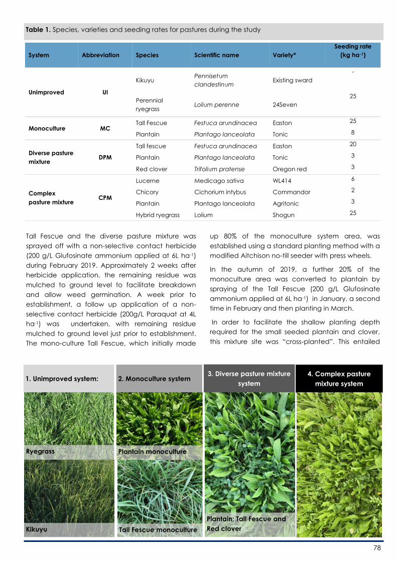
78
Tall Fescue and the diverse pasture mixture was
sprayed off with a non-selective contact herbicide
(200 g/L Glufosinate ammonium applied at 6L ha-1)
during February 2019. Approximately 2 weeks after
herbicide application, the remaining residue was
mulched to ground level to facilitate breakdown
and allow weed germination. A week prior to
establishment, a follow up application of a non-
selective contact herbicide (200g/L Paraquat at 4L
ha-1) was undertaken, with remaining residue
mulched to ground level just prior to establishment.
The mono-culture Tall Fescue, which initially made
up 80% of the monoculture system area, was
established using a standard planting method with a
modified Aitchison no-till seeder with press wheels.
In the autumn of 2019, a further 20% of the
monoculture area was converted to plantain by
spraying of the Tall Fescue (200 g/L Glufosinate
ammonium applied at 6L ha-1) in January, a second
time in February and then planting in March.
In order to facilitate the shallow planting depth
required for the small seeded plantain and clover,
this mixture site was “cross-planted”. This entailed
System Abbreviation Species Scientific name Variety*
Seeding rate
(kg ha-1)
Unimproved UI
Kikuyu Pennisetum
clandestinum Existing sward
-
Perennial
ryegrass Lolium perenne 24Seven
25
Monoculture MC Tall Fescue Festuca arundinacea Easton 25
Plantain Plantago lanceolata Tonic 8
Diverse pasture
mixture DPM
Tall fescue Festuca arundinacea Easton 20
Plantain Plantago lanceolata Tonic 3
Red clover Trifolium pratense Oregon red 3
Complex
pasture mixture
Lucerne Medicago sativa WL414 6
CPM Chicory Cichorium intybus Commandor 2
Plantain Plantago lanceolata Agritonic 3
Hybrid ryegrass Lolium Shogun 25
Table 1. Species, varieties and seeding rates for pastures during the study
1. Unimproved system:
Ryegrass
Kikuyu
2. Monoculture system 3. Diverse pasture mixture
system
Plantain; Tall Fescue and
Red clover
Plantain monoculture
Tall Fescue monoculture
4. Complex pasture
mixture system

79
planting the Tall Fescue parallel to the length of
grazing strips (i.e. from front to back), followed by
the plantain/red clover mixture perpendicular to this
(right to left).
The perennial ryegrass on the kikuyu-ryegrass site
was established by grazing the area down to a
height of 50 mm, mulching the remaining stubble to
ground level and planting the perennial ryegrass
with a modified Aitchison no-till seeder with press
wheels.
The kikuyu-ryegrass pasture was over-sown on an
annual basis (2019 and 2020) as is common practice
in the region, motivated by the poor persistence
and resultant decline in yield of ryegrass that occurs
from year 1 to year 2, even in pure swards under
cutting (van der Colf et al. 2016). In addition, during
the summer of year 1 (January 2020), 20% of the
kikuyu-ryegrass platform was identified as severely
degraded due to the ingression of E. plana. This
area was sprayed of and planted to perennial
ryegrass in March.
The fescue, plantain and mixture pastures were not
over-sown during the autumn of year 1, as
composition in terms of sown species was deemed
to be acceptable. However, a decision was made
to increase the plantain component within the
monoculture system to 50% of the system area for
year 2. The earmarked area was thus sprayed off
and plantain planted using no-till methods in March
2019.
The complex pasture mixture was established in
autumn of 2020. Establishment methods was similar
to that of the DPM, with planting taking place from
mid-April 2020.
Trial animals
Each system was allocated its own “mini-herd” of
animals, selected to maintain days in milk (DIM) at
approximately 150 and provide a constant flow of
animals into and out of the system. Milk yield and
milk composition form the previous lactation were
used to block animals. Each system was allocated
24 animals in milk and 6 dry animals (25% of herd). As
animals in the “milk herd” are dried off, they will be
replaced by animals from the systems’ “dry herd” as
they calve. This may result in periods when the
pasture area for each system is stocked below or
above the 24 animals/system.
Pasture parameters
Pasture yield (kg DM ha-1)
Dry matter production of the pasture treatments was
estimated using the rising plate meter (Stockdale
1984, Fulkerson 1997). Calibration equations were
developed for each pasture type by cutting
samples on monitor strips as per (t’Mannetjie 2000)
to a height of 50 mm. Linear and curvilinear
relationships between herbage mass and pasture
height were determined and best fit equations used
to calculate available herbage mass from pre-
grazing height readings per grazing strip.
The estimated pre-grazing yield will also be used for
pasture allocation purposes (see section on “Pasture
allocation and conservation”).
Botanical composition (%)
Botanical composition was estimated by placing
three 0.098 m2 rings randomly within a sub-plot on
System Sown components Volunteer/weed grasses Broadleaf weeds Volunteer legumes
UI Kikuyu
Ryegrass
Paspalum urvillei*
Eragrostis plana*
Sporobolus africanus*
Bromus catharticus*
Poa pratensis*
Other*
All All
DPM Tall Fescue
Plantain
Red clover
Same as above* (UI)
Ryegrass
All White clover
Trefoil
CPM Lucerne
Plantain
Chicory
Ryegrass
Same as above* (UI)
All White clover
Trefoil
MC Plantain site Same as above* (UI)
Ryegrass
All White clover
Trefoil
Fescue site Same as above* (UI)
Ryegrass
All All
Table 2. Components into which botanical composition samples will be fractioned

80
monitor strips before grazing/cutting and cutting
samples to a height of 50 mm above ground during
each grazing cycle. The three samples were pooled,
thoroughly mixed; a grab sample of approximately
500 g taken and then separated into the relevant
fractions for each pasture type as described in Table
2.
Animal parameters
Cows were milked twice daily at, 07:00 and 15:00,
utilising a 20 Point Waikato/Afikim swing over milking
machine with electronic meters. The machine is fully
automated with weigh-all electronic milk meters
that will allow daily milk production of each
individual cow to be measured.
Milk composition was determined on an
approximately monthly basis from a 24 mL
composite morning and afternoon milk sample of 16
mL and 8 mL, respectively. Samples will be analysed
for butterfat (BF), lactose and milk urea nitrogen
(MUN) content (Milkoscan FT 6000 analyzer; Foss
Electric, Denmark) by Merieux Nutriscience Pty (Ltd)
(Stellenryk Building, Constantia Square Office Park,
526 16th Street, Randjespark, Midrand, 1685). In
addition, daily milk composition in terms of milk
protein, lactose and fat will be available as
determined by the Afimilk milking system.
Pasture and grazing management
Pasture allocation
Each system was managed as a self-sustaining,
closed system, with pasture allocated to each group
following the morning and afternoon milking
according to available pasture biomass (kg DM ha-
1). Pasture biomass available above 50 mm was
determined per sub-plot from RPM readings and
calibrations determined during the study for each
sward type. Pasture was allocated at a rate of 10 kg
DM cow-1 day-1 (approximately 2% of body weight),
with a fresh piece of pasture provided at a rate of 5
kg DM cow-1 after each milking. On the MC system,
animals will be allocated plantain according to the
proportional availability of the pasture within a
period, with the rest of the intake allocated to Tall
Fescue. Cows receive 2 kg of dairy concentrate at
each milking, equating to a total of 4kg cow-1 day-1.
Weekly farm walks and fodder flow
management
In order to facilitate ease of management of fodder
flow within the respective systems, pasture will be
measured on a weekly basis for the entire study site.
For this purpose, grazing strips were allocated to 0.5
ha monitoring blocks on which average leaf number
and pasture height will be determined using a RPM.
Based dry matter yield on a farmlet scale and the
estimated pasture requirement for animals, it was
determined whether pasture availability on the
pasture platform was in excess of animal
requirements (surplus) or lower than requirements
(shortfall). The following strategies were followed
under these circumstances:
Shortfall in winter of year 1: Animals will be
supplemented with bought in feed in the form of
lucerne hay.
Shortfall in year 2 and 3: Grass silage from system
fed to cow groups in isolation. Any shortfall
beyond silage will be met by Lucerne.
Surplus: Area will be cut to make wrapped grass
silage. Plantain will not be cut for silage, with
allocation rate (% of intake) adjusted upwards as
yield increases.
The data collected on the above parameters (silage
made, bales fed and feed bought in) will allow for
the determination of fodderflow dynamics within the
tree systems.
Fertilisation
Corrective fertilisation application for the entire
project site will be based on annual soil sample
analysis results for the 0-100 mm soil depth and the
recommend soil nutrient levels as per Beyers (1973).

81
Based on literature studies and experiences from
current small plot cutting trials on Outeniqua with
pure forage herb and grass/herb swards, nitrogen
was applied at 30 kg N/ha after each grazing.
Results and Discussion
Pasture yield
The total seasonal pasture yield during year 1 and
year 2 of the pasture systems is shown in Table 3.
Due to the lack of replication of farmlets, data
cannot be statistically compared. However, the
data does show that the DPM had the highest
pasture yield during year 1, likely due to it also
achieving the highest seasonal pasture yield from
winter to summer. The highest total annual yield
during year 2 was for the KIK-RYE system, driven by
high summer and autumn yields. Consideration
should, however, be given to the trend of forage
quality decline often observed in kikuyu pastures
during late summer and autumn. This could thus
offset the advantages of high pasture yields in terms
of milk production.
Grazing capacity
The mean monthly grazing capacity of the four
systems during year 1 and year 2 are shown in Figure
1 and Figure 2, respectively.
Grazing capacity showed strong seasonal trends. In
terms of winter grazing capacity during year 1, all
systems had a relatively low, but similar grazing
capacity. However, from mid-spring to early
summer, the DPM system had a higher grazing
capacity than the other systems. The KIK-RYE system
had a higher grazing capacity from the middle of
summer to autumn in year 1.
During year 2, the grazing capacity of the KIK-RYE
Season Winter Spring Summer Autumn Annual
Ye
ar 1
MC 3984 4367 3434 2837 14622
DPM 4017* 5435* 4340* 3140 16932
CPM
KIK_RYE 3070 4003 3695 3846* 14207
Ye
ar 2
MC 2519 3535 3718 3451 13224
DPM 2849 3883 4253 3080 14064
CPM 2434 6851 4138 3997 17420
KIK_RYE 2967 4470 6393 4641 18470
Season Winter Spring Summer Autumn Annual
Ye
ar 1
MC 3204 7621 6904 3472 21201
DPM 2462 8182 7992 4459 23095
CPM
KIK_RYE 3050 6820 7058 4079 21007
Ye
ar 2
MC 3089 6461 5331 3477 18358
DPM 3447 7489 7684 4687 23307
CPM 2247 7816 6699 5301 22064
KIK_RYE 3309 8538 9905 4862 26613
Table 4. Total seasonal and annual milk yield per ha (kg milk/ha) for different pasture systems
MC: Monoculture (Fescue + Plantain) DPM: Diverse pasture mixture (Fescue/plantain/red clover) CPM: Complex pasture
mixture (Lucerne/plantain/chicory/ryegrass)
MC: Monoculture (Fescue + Plantain) DPM: Diverse pasture mixture (Fescue/plantain/red clover) CPM: Complex pasture
mixture (Lucerne/plantain/chicory/ryegrass)
Table 3. Total seasonal and annual pasture yield (kg DM/ha) for different pasture systems

82
Figure 1. Monthly grazing capacity of the diverse pasture mixture, monoculture, kikuyu-ryegrass s and
complex pasture mixture systems during year 1
Figure 2. Monthly grazing capacity of the diverse pasture mixture, monoculture, kikuyu-ryegrass s and
complex pasture mixture systems during year 2

83
Figure 3. Monthly milk yield per cow (kg/cow/day) of the mixture, monoculture and kikuyu-ryegrass systems
during year 1
Figure 4. Monthly milk yield per cow (kg/cow/day) of the diverse mixture, monoculture, kikuyu-ryegrass and
complex pasture mix systems during year 2

84
system was higher than the other systems from spring
through to autumn. This data clearly shows that
grazing capacity can be highly variable over
seasons and years, driven by variable growth rates,.
In turn, growth rates may not only be system
dependant, but also driven by climatic and
management factors.
Milk yield
The mean milk yield per cow (kg/cow/day) for the
pasture systems during year 1 and year 2 is shown in
Figure 3 and 4, respectively.
During year 1, the milk yield per cow was higher for
the cows grazing the DPM system from October to
May. During year 2, the highest yielding system was
more varied over months, but both the DPM and
CPM had a higher milk yield per cow from January
to May than the KIK-RYE and MC systems. Thus, it
appears that the inclusion of a legume and forage
herb in a pasture mixture could improve milk yield
per cow during summer and autumn compared to
kikuyu-ryegrass pastures.
The total seasonal and annual milk yield of the
pasture systems is shown in Table 4. As expected,
milk yield per ha during the first two years, was
driven strongly by pasture yield, and in turn by
grazing capacity. As result, the highest annual milk
yield per ha was for the DPM system in year 1 and
the KIK-RYE system in year 2.
Farm simulation
The challenge with the data presented up to this
point, such as milk yield per ha, is that it does not
take into consideration that farms are often stocked
at a constant rate. As such it neglects to show how
a system may impact:
pasture and milk yield at a average grazing
capacity for the system (i.e. fixed stocking
rate)
Fodder-flow dynamics
Efficiency parameters related to concentrate
(g concentrate/kg milk) and nitrogen (kg DM/
kg N) utilisation, which in turn is affected by
average grazing capacity of the system over
a year
On this premise, a farm simulation was done to
determine farm productivity for the three systems.
Assumptions for the simulation analysis were:
Each farm was 300 ha in size (dairy platform)
The whole farm was planted to the same
system
Farms would be stocked at the average
annual grazing capacity determined over the
two years of the farmlet study (Table 4)
Animals would receive a constant rate of
concentrate of 4 kg concentrate/cow/day
throughout the year Pastures would be
fertilised at 33 kg N/ha after each grazing
In addition, to determine whether a combination of
systems, rather than just one system applied across
the entire farm, could improve whole farm
productivity, a fourth “farm”, referred to as
“COMBINED” was analysed. This farm was divided
into three, and a 1/3 of the farm allocated to each
of the systems.
Figure 5 shows ow the data from the farmlet study
was used to to calculate the parameters for the
farm simulation.
The results from this analysis is shown in Table 5. As
can be seen, different systems performed well for
Index values Farm analysis Farmlet study data
Pasture yield (kg DM/ha)
Grazing intervals (days)
Milk yield (kg/cow/day)
Pasture yield (t DM/year)
Milk yield (t milk/year)
Pasture conserved (t DM/year)
Conserved feed required (t DM/year)
Nitrogen applied (t/year)
Concentrate fed (t/year)
NUE (kg DM/kg N)
Concentrate use efficiency (g C/kg milk)
Figure 4. Methodology used to do whole farm analysis and construct index values
Make data more palata-
ble
Favorable parameter =
others ÷ highest
Unfavorable parameter =
others ÷ lowest

85
Parameter Units MONOC FESC.PL MIX KIK.RYE COMBINED
Grazing capacity Cows/ha 3.58 3.84 4.93 3.90
Milk cows in herd 1074 1152 1318 1171
Concentrate/cow/day kg/cow/day 4 4 4 4
Nitrogen after grazing kg/ha 33 33 33 33
Ye
ar 1
Pasture yield t /year 3558 3639 3156 3451
Milk yield t/year 6128 6974 7632 6844
Conserved feed req. t/year 528 640 1408 878
Pasture Conserved t/year 677 574 172 486
Nitrogen applied t/year 91 87 87 88
Concentrate fed t/year 1568 1683 1924 1708
NUE kg DM/kg N 39 42 36 39
CUE g C/kg milk 256 241 252 250
Ye
ar 2
Pasture yield t /year 4668 3715 4227 4203
Milk yield t/year 6023 7028 7168 6687
Conserved feed req. t/year 272 456 854 590
Pasture Conserved t/year 767 544 1022 798
Nitrogen applied t/year 98 105 90 97
Concentrate fed t/year 1568 1683 1924 1708
NUE kg DM/kg N 48 35 47 43
CUE g C/kg milk 260 239 268 255
Table 4. Whole farm simulation based on farmlet study data for three pasture systems on a 300 ha farm
NUE: Nitrogen use efficiency CUE: Concentrate use efficiency SHADED = MOST FAVOURABLE VALUE
Table 4. Index values for whole farm simulation based on farmlet study data for three pasture systems on a 300 ha farm

86
different parameters and it becomes difficult to
determine which would do well overall. In order to
simplify the analysis further, the data was normalised
to draw up index values. When interpreting index
values, the following should be kept in mind:
Index values do not have units, and
function solely to compare parameters
relative to each other
For this paper, a higher index value
indicates a more favourable performance
for a specific parameter
During year one, the total index value (individual
values summed) of the monoculture and diverse
pasture mixture farm was the highest. This was
primarily a result of both systems having high index
values for conserved feed required (so less feed is
required to supplement pasture) and the amount of
fodder conserved (so more pasture could be cut for
silage) on farm. A similar trend was observed in year
2, when the highest index value was again for the
monoculture system. This is an interesting
observation, since total annual pasture yield (kg
DM/ha) showed that the mixture system was highest
yielding in year 1 and the kikuyu-ryegrass system in
year 2. Thus, high yielding systems, stocked at
grazing capacities, could result in poor fodderflow
dynamics on a farm, leading to more conserved
forage having to be bought in during winter months.
In terms of efficiency index values, concentrate use
efficiency was highest for the mixture farm in both
years. This indicates that the pasture itself on the
mixture system (Fescue, plantain and red clover) is
supporting higher milk yields than on the other
pasture types. In this case, forage quality, rather
than quantity is likely driving the productivity of the
system.
One aspect missing from this analysis is the
economic comparison of systems, particularly as it
relates to aspects like pasture renovation costs
(annual vs strategic), concentrate costs (higher
costs at higher stocking rates) and nitrogen costs
(which in this case would be affected by grazing
interval, since rates were constant per grazing
incident).
Conclusion
Results reported in this paper are still very
preliminary, but do indicate that the inclusion of
plantain, chicory, lucerne and Tall Fescue, whether
in a mixture or as a monoculture, holds the potential
to yield similar or even higher pasture and milk per
ha when compared to kikuyu-ryegrass. The inclusion
of forage herbs and legumes, in particular, could
improve milk yield per cow from spring to autumn.
However, the whole farm analysis highlights the
need to consider other factors, such as fodderflow
and efficiency parameters, when deciding on what
system would suit a particular farming system.
References
Box LA, Edwards GR, Bryant RH. 2016. Milk production and
urinary nitrogen excretion of dairy cows grazing
perennial ryegrass-white clover and pure plantain
pastures. Proceedings of the New Zealand Society of
Animal Production 76: 18-21.
Cave LM, Kemp PD, Kenyon PR, Morris ST. Plantain
(Plantago lanceolata) and chicory (Cichorium intybus)
under moisture stress in glasshouse. Proceedings of the
22nd International Grassland Congress. pp.139-140.
Cheng L, McCormick, Hussein AN, Fraslin C, Moonsan Y,
Logan C, Grabot J, Edwards GR. 2015. Urinary nitrogen
excretion, grazing and urination behaviour of dairy
heifers grazing pasture, chicory and plantain in
autumn. Proceedings of the New Zealand Society of
Animal Production 75: 70-73.
Lee JM, Hemmingson NR, Minee EMK, Clark CEF. 2015.
Management strategies for chicory (Chicorium intybus)
and plantain (Plantago lanceolata): impact on dry
matter yield, nutritive characteristics and plant density.
Crop and Pasture Science 66:168 – 183.
Lowe KF, Bowdler TM. 1995. Growth, persistence, and rust
sensitivity of irrigated, perennial temperate grasses in
Quennsland subtropics. Australian Journal of
Experimental Agriculture, 35,571-8
Mineé EMK, Waghorn GC, Lee JM, Clark CEF. 2017.
Including Chicory and plantain in perennial ryegrass/
white clover-based diet of dairy cattle in late lactation:
Feed intake, milk production and rumen digestion.
Animal Feed Science and Technology 227: 52-61.
Moorhead AJE, Piggot GJ. 2009. The performance of
pasture mixes containing “Ceres Tonic” plantain in
Northland.. Proceedings of the New Zealand Grassland
Association 71: 195-199.
Murrison R, Scott JM. 2013. Statistical methodologies for
drawing causal inference from an unreplicated farmlet
experiment conducted by the Cicerone project.
Animal Production Science 53:643-648.
Nie Z, Miller S, Moore G, Hackney B, Boschma S, Reed KFM,
Mitchell M, Albertsen TO, Clark S, Craig AD, Kearney G,
Li GD, Dear BS. 2008. Field evaluation of perennial
grasses and herbs in southern Australia 2. Persistence,
root characteristics and summer activity. Australian
Journal of Experimental Agriculture, 48:424-435.
87
Scott JM, Munro M, Rollings N, Browne W, Vickery PJ, Macgregor C, Donald GE, Sutherland H. 2013a. Planning for whole
farm systems research at a credible scale: subdividing land into farmlets with equivelant initial conditions. Animal
Production Science 53: 618-627.
Scott JM, Behrendt K, Colvin A, Scott F, Shakhane LM, Guppy C, Hoad J, Gaden CA, Edwards C, Hinch GN, Cacho OJ,
Donald GE, Cottle D, Coventry T, Williams G, Mackay DF. 2013b. Integrated overview of result from a farmlet
experiment which compared the effects of pasture inputs and grazing management on profitability and sustainability.
Animal Production Science 53: 841-855.
Stockdale CR. 1984. Evaluation of techniques for estimating the yield of irrigated pastures intensively grazed by dairy
cows. II. The rising plate meter. Australian Journal of Experimental Agriculture and Animal Husbandry 24: 305-311.
`t Mannetjie L. 2000. Measuring biomass of grassland vegetation. In: Field and Laboratory methods for grassland and
animal measurement. Eds: `t Mannetjie L, Jones RM. CAB International. Wallingford, UK.
Totty VK, Greenwood SL, Bryant RH, Edwards GR. 2013. Nitrogen partitioning and milk production of dairy cows grazing
simple and diverse pastures. Journal of Dairy Science 96:141-149.
van der Colf J, Ammann SB, Zulu LB, Lombard MM. 2016. Pasture dry matter yield of perennial ryegrass and ryegrass
hybrids in the southern Cape. Outeniqua Research Farm Day 2016 Booklet. 21-27.
Van Eekeren N, Bos M, De Wit J, Kiedel H, Bloem J. 2010. Effect of individual grass species and grass species mixtures on
soil quality as related to root biomass and grass yield. Applied Soil Ecology 45: 2715-283.
Woodward SL, Waugh CD, Roch CG, Fynn D, Phillips J. 2013. Are diverse species mixtures better pastures for dairy farming.
Proceedings of the New Zealand Grassland Association.

88
The effect of partial replacement of perennial ryegrass
with plantain pasture and concentrate level on milk
production and milk composition of Jersey cows in
spring
Robin Meeske*, Bertus Myburgh and Pieter Cronje
Western Cape Department of Agriculture, Outeniqua Research Farm, George
Corresponding author email: [email protected]
Introduction
Kikuyu/ryegrass pasture under irrigation is commonly
used as forage for dairy cows in the southern Cape.
Plantain however has become more popular and is
planted in pure stands or as part of a pasture mix.
Plantain has a high production potential, low fibre
content and high feeding value, but is low in
effective fibre. This may result in less rumination and
lower rumen pH levels. The response on concentrate
feeding is expected to change depending on level
of concentrate feeding and the proportion of
ryegrass and plantain in the total diet. Concentrates
are relatively expensive compared to pasture and
often contain 50-80% maize. As the level of
concentrate feeding to cows increases the rumen
pH is expected to be lower. When rumen pH gets
below 5.8, fibre digestion may be compromised.
Most research on plantain has been done in New
Zealand where concentrate supplementation to
cows is not common. Very limited research is
available on effective concentrate
supplementation to cows that consume plantain as
50% of their forage intake.
Aim
The aim of the study was to determine the effect of
partial replacement of ryegrass pasture with
plantain pasture during spring on milk production
and milk composition at a low and a high level of
concentrate feeding.
Materials and methods
The study was conducted during spring 2020
(September/October) at the Outeniqua Research
Farm, situated near George in the Western Cape
province of South Africa (22º 25´ 16ˊˊE and 33˚ 58ˊ
38ˊ´S). Nine hectares kikuyu/ryegrass pasture under
permanent irrigation was over-sown with perennial
ryegrass (Lolium multiflorum) cv. Base at 20kg/ha in
May 2020. Plantain (cv. Agritonic) was planted at
9kg/ha on five hectare under irrigation during April
2019 and another 3 ha was planted in March 2020.
The study took place during September/ October
2020 and consisted of a 14 day adaptation and 44
day measurement period. Fertilizer was applied at
42kg N after each grazing (150kg/ha limestone
ammonium nitrate (LAN) containing 28% nitrogen).
Pasture was irrigated according to soil moisture
probe readings. The grazing cycle varied from 21 to
25 days depending on pasture growth rate. Sixty
Jersey cows from the Outeniqua Research Farm
were used in a randomized block design with four
treatments (15 cows/treatment). The cows were
blocked according to milk production (of the
previous three weeks, 20.7±1.76 kg), lactation

89
number (4.1±1.78) and days in milk (98±43.5 DIM)
and were randomly allocated to one of four
treatments:
1. Cows grazed kikuyu/ryegrass pasture day
and night with supplementation of 3.5kg
concentrate (RGRG 3.5).
2. Cows grazed kikuyu/ryegrass pasture day
and night with supplementation of 7kg
concentrate (RGRG 7).
3. Cows grazed plantain pasture during the
day and kikuyu/ryegrass pasture during the
night with supplementation of 3.5kg
concentrate (RGPL 3.5).
Cows grazed plantain pasture during the day and
kikuyu/ryegrass pasture during the night with
supplementation of 7kg of concentrate (RGPL 7).
The dairy concentrate (DM 89%, 11MJ ME/kg, CP
12%, Ca 1% and P 0.4% on as is basis) was fed in the
dairy parlour during milking at either 3.5kg/cow/day
or 7kg/cow/day divided in equal portions between
the two milkings. Cows on the plantain treatments
were drafted after morning milking using a drafting
gate to separate them from cows on ryegrass
treatments. These cows strip grazed plantain pasture
during the day while the other cows grazed kikuyu/
ryegrass pasture. All cows strip grazed kikuyu/
ryegrass pasture as one group during the night.
Cows were milked at 06h00 and 14h30 and grazed
24 hours per day (except for milking times). Clean
water was provided (ad Libitum). Cows were
marked with a coloured tag and light chain
hanging from the neck indicating the specific
treatment. Pasture (plantain and kikuyu/ryegrass)
and concentrate samples were collected weekly.
Concentrate samples were pooled for every two
weeks resulting in 4 concentrate samples. Pasture
samples were collected weekly by randomly cutting
four circles of 35.4 cm in diameter at a height of 3
cm above the ground. Samples were dried at 60ºC
for 72 hours to determine the % DM and pooled for
every two weeks resulting in four ryegrass and four
plantain samples. All samples were milled though a
1mm screen with a Retsch GmbH5657 Laboratory
mill (Retch GmbH 5657 Haan, West Germany) and
stored pending analysis. The concentrate and
pasture samples were analysed for DM, ash, crude
protein, metabolisable energy, NDF, ADF, Ca, P, Mg,
K, Na, Fe, Zn, Cu and Mn.
The pasture height was determined by using the
rising plate meter (RPM) (Filip’s folding plate pasture
meter, Jenquip, Rd 5, Fielding, New Zealand). The
pasture height of each grazing strip was determined
by taking 100 RPM readings before and after
grazing. Pasture was allocated at 12-14 kg DM/
cow/day. An after grazing pasture height of 10-12
on the RPM was targeted to ensure that pasture was
not limiting.
Cows were weighed and body condition scored at
the beginning and at the end of the study on two
consecutive days before afternoon milking. Body
condition score (BCS) of cows was determined on a
scale of 1 to 5, where 1 is thin and 5 is fat. Cows
were milked using a 20 Point Waikato/Afikim swing
over milking machine with electronic meters. Milk
production was recorded during each milking with
the Afikim milk meter and management system.
Composite milk samples (Ratio 8 ml: 16 ml,
afternoon: morning milking) (06h00 and 14h30) were
collected every two weeks. Milk samples were
analysed for fat, protein, lactose, somatic cell count
(SCC) and MUN using a Milkoscan FT 6000 machine
(Foss Electric, Denmark).
Results and discussion
The chemical composition of ryegrass, plantain and
concentrate fed to cows is presented in Table 1. The
crude protein content of the plantain was lower
and the NDF content higher than expected.
Plantain did contain a higher level of Ca and lower
level of K than ryegrass. The energy value of ryegrass
and plantain was similar. The RPM height before and
after grazing was 32.7±7.60 and 10.7±2.40 for
ryegrass and 29.7±7.17 and 9.53±3.05 for plantain
respectively.
Milk production, milk composition and live weight
gain of cows is presented in Table 2. The average
live weight of cows was 399 ± 36.5kg at the start of
the study.
No significant interaction (P>0.05) was found
between pasture and concentrate treatments for
any of the parameters and therefor the main effects
of pasture and concentrate were presented. Milk
production of cows grazing ryegrass or ryegrass and
plantain was similar (p = 0.19) at 18.8 and 19.4 kg
milk per day respectively. Four percent fat

90
Table 1. Composition (% of DM) of ryegrass pasture, plantain pasture and concentrate fed to cows during spring.
Composition ( % of DM) Ryegrass pasture Plantain pasture Concentrate
DM% 12.6 12.4 88.9
Crude protein% 19.8 13.6 11.5
ME MJ/kg 10.7 10.8 12.7
NDF % 47.9 38.5 14.8
ADF% 30.1 33.2 6.66
Ca% 0.52 1.38 1.40
P% 0.53 0.32 0.50
Mg% 0.38 0.39 0.32
K% 3.68 2.18 1.06
Na % 1.43 2.51 0.23
Mn ppm 47.2 33.4 198
Cu ppm 7.24 8.02 19.4
Fe ppm 228 154 136
Zn ppm 41.3 44.7 201
Table 2: Milk production, milk composition and live weight gain of Jersey cows grazing ryegrass or ryegrass and plantain
in spring supplemented with 3.5 or 7kg concentrate/cow/day.
Pasture Treatment Concentrate Treatment
Parameter RGRG RGPL P-value 3.5kg 7.0kg P-value SEM
Milk production (kg/cow/day) 18.8 19.4 0.19 18.4 19.8 0.001 0.30
FCM 4% (kg/cow/day) 21.4 21.7 0.63 20.8 22.2 0.01 0.39
Milk fat % 4.93 4.80 0.30 4.89 4.84 0.66 0.090
Milk protein % 3.79 3.72 0.19 3.75 3.76 0.77 0.040
Milk lactose % 4.65 4.66 0.87 4.63 4.69 0.12 0.025
MUN mg/dl 9.11 5.81 <0.001 8.13 6.79 0.006 0.343
Live weight
gain (kg) 21.4 22.6 0.68 21.3 22.7 0.61 1.90
FCM= Fat corrected milk; MUN= milk urea nitrogen; RGRG = cows grazed ryegrass day and night; RGPL= cows grazed
ryegrass at night and plantain during the day.

91
corrected milk did not differ (p = 0.69) and was 21.4
and 21.7 kg per cow per day for RGRG and RGPL
pasture treatments. Milk production and 4 % fat
corrected milk (FCM) increased significantly due to
higher concentrate feeding and was 18.4 and 19.8
kg milk/cow/day (p = 0.001) and 20.8 and 22.2 kg
FCM/cow/day (p = 0.01) for cows fed 3.5 or 7 kg/
day. The response on concentrate feeding was low
at only 0.40 kg milk per kg concentrate fed as
concentrate feeding increased from 3.5 to 7 kg/
cow/day. Milk composition was not significantly (p >
0.05) affected by pasture or concentrate
treatments.
Economic implications
Economic implications of level of concentrate
feeding during spring is presented in Table 3. When
pasture quality and availability is high, response on
concentrate feeding will be lower and feeding less
concentrate may be more profitable.
Farmers should approach level of concentrate
feeding to cows in balance with pasture quality and
availability. Feeding less concentrate when pasture
quality is high and more concentrate when pasture
quality is low may result in improved profitability.
Conclusions
Partial replacement of ryegrass with plantain during
spring, when pasture quality is high, did not increase
milk production. Farmers should though consider
feeding lower levels of concentrate to cows during
spring when pasture quality and availability is high.
In our study the return of only 0.4kg milk per kg of
concentrate when increasing concentrate feeding
from 3.5 to 7kg/cow/day resulted in lower profit.
Table 3. Economic implications of level of concentrate feeding for cows grazing high quality pasture during spring.
Parameter 3.5 kg Concentrate 7 kg of concentrate
Milk production kg/cow/day 18.4 19.8
Milk income R/cow/day R114.08 R122.76
Cost of concentrate R20.30 R40.60
Pasture intake kg/cow/day (estimation) 10 8
Cost of pasture R/cow/day R15.00 R12.00
Margin over feed cost R/cow/day R83.78 R74.16
Increase in margin/cow/day feeding less concentrate R9.62
Increase in margin R/month for 400 cows R115 440.00
Assumptions: Cost of pasture R1.50/kg, Concentrate R5.80, Milk price R6.20

92
Milk flocculation: Does feeding more phosphorous to
cows improve milk protein stability?
Robin Meeske1*, Wicus Joubert2, Bertus Myburgh1 and Pieter Cronje1
1Western Cape Department of Agriculture, Outeniqua Research Farm, George
2Nova Feeds
Corresponding author email: [email protected]
Introduction
The processing of milk as UHT or long life milk is
continuously increasing. According to Milk SA, UHT
and Steri Milk comprised 43% of the South African
liquid products market compared to 34% for
pasteurised milk in 2018 (Lactodata, 2020). With a
total milk production of 3 411000 tons in 2018 of
which 62% was processed for the liquid market the
annual production of UHT milk was 909000 tons with
a retail value of approximately R10.9 billion. It is
expected that the demand for UHT milk will grow in
future. During the processing of long life milk or UHT
milk, the milk is subjected to heat treatment. The
casein complex in milk must withstand the heat
treatment and sustain its integrity. If UHT milk is not
stable, protein will precipitate, flocculation occurs
and shelf life of milk is compromised. This is not
acceptable for consumers and milk is rejected
resulting in major financial losses for milk processors.
The alizarol test is used to estimate the heat stability
of milk. Milk has to pass the 76 % alizarol test to be
suitable for processing as UHT milk. The biggest
challenge with unstable milk occurs during the late
summer and autumn when pasture quality is lower
and cows also experience heat stress. Phosphorous
plays a key role in stability of protein micelles in milk.
Sanchez et al. (1994) showed that phosphorous
supply to the udder was reduced by 50% during
heat stress. This may partially explain why the
problem of unstable milk is more prominent from
February to April. Fagnani et al. (2014) reported
lower levels of phosphorous in unstable milk
compared to stable milk. This was also found in a
previous study at Outeniqua Research farm. Forar et
al. (1982) found that inorganic phosphate in milk
was lower during summer compared to winter. The
mineral content of milk plays an important role in the
stability of the milk protein and more specific the
casein micelle (Tsioulpas et al., 2007). Supplementing
mono calcium phosphate at 80 g/cow/day has
improved protein stability of milk on some farms in
the Tsitsikamma in the past.
Aim
To determine if changing the Ca:P ratio in the diet of
cows grazing kikuyu pasture in late summer from 2:1
tot 1:1 will increase phosphorous content of milk and
improve protein stability.

93
Material and Methods
The study was conducted during February/March
2021 on the Outeniqua Research Farm, situated
near George in the Western Cape province of South
Africa (22º 25´ 16ˊˊE and 33˚ 58ˊ 38ˊ´S). Twenty
hectares irrigated kikuyu/ryegrass pasture was used
in the study. Fertilizer was applied at 33kg N after
each grazing (150kg/ha 1:0:1 containing 22%
nitrogen). Pasture height was measured with a rising
plate meter (RPM) and pasture was allocated at
12kgDM/cow/day. A pasture height before and
after grazing on the RPM of 25 and 12 respectively
was targeted to ensure proper pasture utilization as
well as sufficient pasture allocation.
Eighty multiparous Jersey cows of the Outeniqua
Jersey herd were be randomly allocated to one of
two treatments:
1. Dietary Ca:P ratio of 2:1
2. Dietary Ca:P ratio of 1:1
The study was a cross-over design with two
treatments and two periods (40 cows per treatment
during each period). The different Ca:P ratios were
achieved by feeding two different dairy
concentrates as shown in Table1.
Concentrates were mixed and pelleted by Nova
Feeds, George and delivered in bulk into two silos.
The Ca and P content of pasture was expected to
be the same at 0.4%. With supplementation of 6kg of
concentrate, the Ca:P ratio of the total diet should
be 2:1 and 1:1 for the control and high P treatment
respectively. Cows were adapted to diets for 14
days followed by a measurement period of 7 days in
period, after which treatments were switched for
period 2. Concentrates were fed in the dairy parlour
during milking at 6kg/cow/day divided between the
morning and afternoon milking. Composite morning
and afternoon milk samples were collected on day
1, 3 and 5 of each measurement period. Milk
production was recorded daily and cows were
weighed and condition scored at the start and end
of each period. Milk samples were analysed for fat,
protein, lactose, MUN, SCC, Ca, P and Alizarol level
passed (72, 74, 76, 78 and 80%) as well as Ca, P, Mg,
K and Na content. Pasture and concentrate
samples were collected during each measurement
period on day 1, 3 and 5. A total of 6 pasture
samples (2 per sampling day) and 6 concentrate
samples (3 for Control and 3 for high P treatment)
were analysed per period for DM, OM, IVOMD, CP,
Ca, P, Mg, K, Na, Zn, Cu, Mn, Fe. Milk samples taken
were 240 (80 cows X3 samples) for each
measurement period resulting in a total of 480 milk
samples collected and analysed during the study.
Table 1. Concentrates differing in P content fed to cows grazing kikuyu/ryegrass
Ingredient Control High P
Hominy chop 10 10
Maize grain 59.9 59.9
Wheaten bran 10 8,2
Soybean oilcake 12 12
Molasses syrup 4 4
Feed lime 2.9 1.25
Mono-CaP 0 3.35
MgO 0.3 0.3
Salt 0.5 0.5
Urea 0.3 0.4
Premix 0.1 0.1
Total 100 100
Composition
ME MJ/kg 12.1 12.0
Crude Protein % 15.0 15.2
NDF % 16.5 16.3
Ca % 1.21 1.21
P % 0.49 1.18

94
Results and discussion
The composition of the concentrates supplemented
at 6kg/cow/day and pasture offered to Jersey cows
is presented in Table 2. The high P concentrate
contained 1.22% P compared to 0.43% P of the
control concentrate. The estimated Ca:P ratio in the
total diet was 1.8:1 and 1:1 for the control and high P
treatment respectively. The intake of P was 43g/
cow/day higher on the high P treatment compared
to the control. We thus succeeded in substantially
increasing P intake by cows on the high P treatment.
The % of cows that failed the 72 to 80% alizarol test is
presented in Table 3. The incidence of flocculation
did not differ between the control and high P
treatment at any of the alizarol levels tested. It is
interesting to note that 33% and 35% of cows failed
the 76% alizarol test on the control and high P
treatment respectively. The incidence of
flocculation was therefore substantial in both the
control and the high P treatment.
During the study we did not experience very high
ambient temperatures and cows were not
subjected to any nutritional stress. The pasture was
of good quality (Table 2) and availability of pasture
was sufficient as indicated by the rising plate meter
reading of 27±5.1 and 9.14±1.02 before and after
grazing respectively.
Table 2. Composition of concentrates supplemented and pasture offered to Jersey cows
Parameter (% of DM) Control concentrate
n=6
High P concentrate
n=6
Pasture
n=12
DM% 89.8±0.20 90.4±0.28 13.0±2.32
Ash% 7.0±0.16 7.8±0.33 12.2±1.18
Crude protein% 13.6±0.62 14.4±0.43 22.7±3013
ME MJ/kg 12.4±0.03 12.4±0.02 10.4±0.19
NDF% 11.9±0.53 10.5±0.54 51.2±2.88
ADF% 4.92±0.05 4.29±0.07 28.1±1.75
Ca% 1.39±0.064 1.30±0.064 0.44±0.050
P% 0.43±0.017 1.22±0.019 0.49±0.051
Mg% 0.41±0.024 0.42±0.050 0.43±0.044
K% 1.30±0.058 1.37±0.027 4.09±0.472
Na% 0.25±0.024 0.26±0.005 0.27±0.135
Mn ppm 215±11.0 214±9.2 47.9±18.5
Cu ppm 9.54±1.69 10.3±1.29 3.99±0.544
Fe ppm 165±25.7 272±17.9 194±38
Zn ppm 103±3.2 104±2.4 23.6±1.82
Table 3. The % of cows that failed the 72, 74, 76, 78 and 80% alizarol test when fed the control or high P concentrate,
n=80.
% Alizarol tested Control High P P-value
72 12.2 9.9 0.41
74 20.9 21.5 0.88
76 33.0 35.2 0.65
78 42.4 46.3 0.44
80 56.6 62.4 0.23

95
Milk production and milk composition of cows fed
control or high P concentrate is presented in Table 4.
Milk production or milk composition was not
affected by increasing the level of P in the diet. The
statistical significant differences in milk protein and
lactose between treatments were very small and
not of any biological significance. The MUN levels
were high indicating that protein feeding was
sufficient.
The average alizarol level passed was not improved
by feeding more phosphorous to cows and the
mineral content of milk was not affected. The P level
in milk compared well with values reported by
Fagnani et al. (2014) on milk with high protein
stability. Mineral content of milk in our study
compared well with values reported by Tsioulpas et
al. (2007) of Ca 129mg/100ml, P 84 mg/100ml, Mg
9.7mg/100ml, Na 54mg/100ml and K 148mg/100ml.
Conclusions
Increasing phosphorous in the diet did not improve
the protein stability of milk in this study. Milk
production and milk composition was not affected.
A third of the cows in the study produced milk that
did not pass the 76% alizarol test and was therefore
not suitable to process as UHT milk on both the
control and high P treatments. Protein stability of milk
is complex as it is affected by both environmental
and nutritional stress as well as the genetics of the
cow.
References
Fagnani, R., Beloti, V and Battaglini, A.P.A., 2014.
Acid-base balance of dairy cows and its
relationship with alcoholic stability and mineral
composition of milk. Pesq. Vet. Bras. 34(5): 398-
402.
Forar, F. L., R. L. Kincaid, R. L. Preston, and J. K. Hillers.
1982. Variation of inorganic phosphate in
blood plasma and milk lactating cows. J. Dairy
Sci. 65:760.
Lactodata 2020. Statistics compiled by the Milk
Producers Organisation. Lactodata, Volume
23 no 1, May 2020, page 26.
Sanchez, W.K., McGuire, M.A, and Beede, D. K.,1994.
Macromineral Nutrition by Heat Stress
Interactions in Dairy Cattle. J. Dairy Sci 77:2051-
2079
Tsioulpas, A., Lewis, M.J. and Grandison, A.S., 2007.
Effect of Minerals on casein micelle Stability of
cow’s milk. J. Dairy Res., 74: 167-173.
Table 4. Milk production and milk composition of cows grazing kikuyu/ryegrass pasture during autumn supplemented with
control and high P concentrate.
Parameter Control High P P-value
Milk production kg/cow/day 16.6 16.7 0.40
4% Fat corrected milk kg/cow/day 19.0 19.1 0.82
Milk fat % 5.03 5.00 0.43
Milk protein % 3.93 3.96 0.012
Milk lactose % 4.56 4.54 0.005
MUN mg/dl 16.9 17.0 0.46
Somatic cell count X 1000 127 136 0.96
Milk pH 6.65 6.67 0.27
Average Alizarol % passed 76.5 76.4 0.65
Milk mineral content
Ca mg/100ml 142 141 0.52
P mg/100ml 77.4 76.9 0.42
Mg mg/100ml 12.8 12.8 0.99
Na mg/100ml 38.4 38.8 0.43
K mg/100ml 136 136 0.95

96
We
ath
er
da
ta:
Ou
ten
iqu
a R
ese
arc
h F
arm
20
19
to
20
21
Da
len
a L
om
ba
rd
We
ste
rn C
ap
e D
ep
art
me
nt
of
Ag
ric
ultu
re,
Re
sea
rch
an
d T
ec
hn
olo
gy
De
ve
lop
me
nt,
Dir
ec
tora
te P
lan
t Sc
ien
ce
s, O
ute
niq
ua
Re
sea
rch
Fa
rm,
P.O
. B
ox 2
4,
Ge
org
e
65
30
Co
rre
spo
nd
ing
au
tho
r e
ma
il: D
ale
na
L@e
lse
nb
urg
.co
m
20
19
2020
2021
January
February
March
April
May
June
July
August
September
October
November
December
January
February
March
April
May
June
July
August
September
October
November
December
January
February
March
April
May
Min
T
15
.8
17
.2
15
.8
13
.4
11
.7
9.3
7
.7
9.6
1
1.8
1
1.9
1
4.6
1
5.0
1
5.7
1
6.0
1
3.3
1
2.5
8
.6
9.8
8
.4
7.2
1
0.1
1
0.0
1
3.2
1
4.3
1
6.9
1
7.7
1
5.2
1
3.8
1
1.3
Ma
x T
2
2.7
2
1.5
2
2.0
2
0.1
2
6.8
2
3.2
1
6.9
1
7.7
2
8.4
1
9.2
2
0.2
2
1.4
2
4.8
2
6.8
2
5.8
2
6.6
2
2.5
2
0.7
2
1.2
1
8.3
2
2.8
2
0.0
2
6.4
2
1.9
2
4.6
2
5.0
2
7.0
2
4.0
2
2.3
Me
an
T
19
.0
19
.8
19
.0
16
.3
15
.7
14
.3
13
.4
12
.9
16
.0
15
.8
17
.3
18
.0
19
.5
20
.1
18
.4
16
.9
15
.3
15
.1
13
.9
12
.4
14
.4
15
.1
17
.3
18
.9
20
.3
20
.1
19
.5
17
.6
15
.5
RF
24
75
56
36
41
29
30
3
58
35
60
32
13
4
37
33
34
53
18
14
51
68
10
1
68
31
38
30
64
42
85
PA
R
20
4
21
5
18
7
14
1
10
9
10
4
12
5
15
5
16
0
20
0
25
6
21
6
18
7
20
2
16
8
16
4
11
8
10
1
11
9
11
9
17
5
19
4
18
8
19
9
20
7
20
8
16
5
15
3
11
4
Min
T =
Min
imu
m t
em
pe
ratu
re (
°C)
rec
ord
ed
in
sp
ec
ific
mo
nth
Ma
x T
= M
axim
um
te
mp
era
ture
(°C
) re
co
rde
d in
sp
ec
ific
mo
nth
Me
an
T =
Me
an
te
mp
era
ture
(°C
) o
f sp
ec
ific
mo
nth
RF =
To
tal R
ain
fall
(mm
) re
co
rde
d in
sp
ec
ific
mo
nth
PA
R =
Me
an
ph
oto
syn
the
tic
ally
ac
tive
ra
dia
ton
re
ad
ing
(W
att
s/m
2)
of
spe
cific
mo
nth

97

98

99

100

101

102
Outeniqua Research Farm l Outeniqua Navorsingsplaas
2020 Information Day l 2020 Inligtingsdag