Information and Computation - COnnecting REpositories · P. Baldan et al. / Information and...
24
Information and Computation 208 (2010) 1169–1192 Contents lists available at ScienceDirect Information and Computation journal homepage: www.elsevier.com/locate/ic Unfolding-based diagnosis of systems with an evolving topology < Paolo Baldan a,∗ , Thomas Chatain b , Stefan Haar b Barbara König c a Dipartimento di Matematica Pura e Applicata, Università di Padova, Italy b LSV, CNRS & ENS de Cachan, INRIA, France c Abteilung für Informatik und Angewandte Kognitionswissenschaft, Universität Duisburg-Essen, Germany ARTICLE INFO ABSTRACT Article history: Available online 20 June 2010 Keywords: Model-based diagnosis Distributed and concurrent systems Partial order methods Graph rewriting We propose a framework for model-based diagnosis of systems with mobility and variable topologies, modelled as graph transformation systems. Generally speaking, model-based diagnosis is aimed at constructing explanations of observed faulty behaviours on the basis of a given model of the system. Since the number of possible explanations may be huge, we exploit the unfolding as a compact data structure to store them, along the lines of previous work dealing with Petri net models. Given a model of a system and an observation, the explanations can be constructed by unfolding the model constrained by the observation, and then removing incomplete explanations in a pruning phase. The theory is formalised in a general categorical setting: constraining the system by the observation corresponds to taking a product in the chosen category of graph grammars, so that the correctness of the procedure can be proved by using the fact that the unfolding is a right adjoint and thus it preserves products. The theory should hence be easily applicable to a wide class of system models, including graph grammars and Petri nets. © 2010 Elsevier Inc. All rights reserved. 1. Introduction The event-oriented model-based diagnosis problem is a classical topic in discrete event systems [1, 2]. Given an observed alarm stream, the aim is to provide explanations in terms of actual system behaviours. Some events of the system are observable (alarms) while others are not. In particular, fault events are usually unobservable; therefore, fault diagnosis is the main motivation of the diagnosis problem. Given a sequence (or partially ordered set) of observable events, the diagnoser has to find all possible behaviours of the model explaining the observation, thus allowing the deduction of invisible causes (faults) of visible events (alarms). The paper [3] provides a survey on fault diagnosis in this direction. Since the number of possible explanations may be huge, especially in the case of highly concurrent systems, it is advisable to employ space-saving methods. In [3, 4], the global diagnosis is obtained as the fusion of local decisions: this distributed approach allows one to factor explanations over a set of local observers and diagnoses, rather than centralising the data storage and handling. We will build here upon the approach of [5] where diagnoses are stored in the form of unfoldings. The unfolding of a system fully describes its concurrent behaviour in a single branching structure, representing all the possible computation steps and their mutual dependencies, as well as all reachable states; the effectiveness of the approach lies in the use of partially ordered runs, rather than interleavings, to store and handle explanations extracted from the system model. < Supported by the RNRT project SWAN No. 03 S 481, INRIA Sabbatical program, the DFG project SANDS, the MIUR project SisteR and the project AVIAMO of the University of Padova. ∗ Corresponding author. E-mail addresses: [email protected] (P. Baldan), [email protected] (T. Chatain), [email protected] (S. Haar), [email protected] (B. König). 0890-5401/$ - see front matter © 2010 Elsevier Inc. All rights reserved. doi:10.1016/j.ic.2009.11.009
Transcript of Information and Computation - COnnecting REpositories · P. Baldan et al. / Information and...

Information and Computation 208 (2010) 1169–1192
Contents lists available at ScienceDirect
Information and Computation
j o u r n a l h o m e p a g e : w w w . e l s e v i e r . c o m / l o c a t e / i c
Unfolding-based diagnosis of systems with an evolving topology<
Paolo Baldana,∗, Thomas Chatainb, Stefan Haar b Barbara König c
aDipartimento di Matematica Pura e Applicata, Università di Padova, Italy
bLSV, CNRS & ENS de Cachan, INRIA, France
cAbteilung für Informatik und Angewandte Kognitionswissenschaft, Universität Duisburg-Essen, Germany
A R T I C L E I N F O A B S T R A C T
Article history:
Available online 20 June 2010
Keywords:
Model-based diagnosis
Distributed and concurrent systems
Partial order methods
Graph rewriting
We propose a framework for model-based diagnosis of systems with mobility and variable
topologies, modelled as graph transformation systems. Generally speaking, model-based
diagnosis is aimed at constructing explanations of observed faulty behaviours on the basis
of a given model of the system. Since the number of possible explanations may be huge, we
exploit the unfolding as a compact data structure to store them, along the lines of previous
work dealing with Petri net models. Given a model of a system and an observation, the
explanations can be constructed by unfolding the model constrained by the observation,
and then removing incomplete explanations in a pruning phase. The theory is formalised
in a general categorical setting: constraining the system by the observation corresponds to
taking a product in the chosen category of graph grammars, so that the correctness of the
procedure can be proved by using the fact that the unfolding is a right adjoint and thus it
preserves products. The theory should hence be easily applicable to a wide class of system
models, including graph grammars and Petri nets.
© 2010 Elsevier Inc. All rights reserved.
1. Introduction
The event-oriented model-based diagnosis problem is a classical topic in discrete event systems [1,2]. Given an observed
alarm stream, the aim is to provide explanations in terms of actual system behaviours. Some events of the system are
observable (alarms) while others are not. In particular, fault events are usually unobservable; therefore, fault diagnosis is the
main motivation of the diagnosis problem. Given a sequence (or partially ordered set) of observable events, the diagnoser
has to find all possible behaviours of the model explaining the observation, thus allowing the deduction of invisible causes
(faults) of visible events (alarms). The paper [3] provides a survey on fault diagnosis in this direction.
Since the number of possible explanationsmay be huge, especially in the case of highly concurrent systems, it is advisable
to employ space-saving methods. In [3,4], the global diagnosis is obtained as the fusion of local decisions: this distributed
approach allows one to factor explanations over a set of local observers and diagnoses, rather than centralising the data
storage and handling.
We will build here upon the approach of [5] where diagnoses are stored in the form of unfoldings. The unfolding of a
system fully describes its concurrent behaviour in a single branching structure, representing all the possible computation
steps and their mutual dependencies, as well as all reachable states; the effectiveness of the approach lies in the use of
partially ordered runs, rather than interleavings, to store and handle explanations extracted from the system model.
< Supported by the RNRT project SWAN No. 03 S 481, INRIA Sabbatical program, the DFG project SANDS, the MIUR project SisteR and the project AVIAMO of
the University of Padova.∗ Corresponding author.
E-mail addresses: [email protected] (P. Baldan), [email protected] (T. Chatain), [email protected] (S. Haar),
[email protected] (B. König).
0890-5401/$ - see front matter © 2010 Elsevier Inc. All rights reserved.
doi:10.1016/j.ic.2009.11.009

1170 P. Baldan et al. / Information and Computation 208 (2010) 1169–1192
In order to provide some intuition about unfoldings, an example of a Petri net and a fragment of its unfolding are reported
in Fig. 1. In the Petri net, for later use, a bold face label is used to denote alarms, i.e., observable transitions. More explicitly,
transitions labelled a, b, c, d are observable, while e, f are not. The unfolding is inductively constructed, starting from the
initialmarking and recording, step after step, any possible firing of a transition,with the tokens it produces. Hence transitions
and places in the unfolding can be seen as occurrences of firing of transitions (events) and of tokens in computations of the
original net. The causal dependencies and conflicts between items of the unfolding are made explicit by the structure of
the unfolding itself. For instance, let us focus on the upper part of the unfolding. The two events labelled a are in conflict,
since they consume a common resource, while the leftmost event labelled a is a cause for the event labelled e. Instead, the
absence of dependencies between the events e and f , means that such events are concurrent and thus they can interleave
in any way.
While [5] and subsequent work in this direction were mainly directed to Petri nets, here we face the diagnosis problem
in mobile and variable topologies. This requires the development of a model-based diagnosis approach which applies to
other, more expressive, formalisms. Unfoldings of extensions of Petri nets where the topologymay change dynamically were
studied in [6,7]. Here we focus on the general and well-established formalism of graph transformation systems.
In order to retain only the behaviour of the system that matches the observation, it is not the model itself that is un-
folded, but the product of the model with the observations, which intuitively represents the original system constrained
by the observation; under suitable observability assumptions, only a finite prefix of the unfolding must be considered. The
construction is carried out in a suitably defined category of graph grammars, where such a product can be shown to be the
categorical product. A further pruning phase is necessary in order to remove incomplete explanations that are only valid for
a prefix of the observations.
Fig. 1. A Petri net (left) and a fragment of its unfolding (right).
Fig. 2. An observation (left) and the corresponding diagnosis net (right).

P. Baldan et al. / Information and Computation 208 (2010) 1169–1192 1171
The steps of the diagnosis procedure can be illustrated, for the Petri net case, by referring to the net in Fig. 1. Assume
that the observation is given by the sequence a b c. The idea consists in representing the observation as a special system, in
this case a Petri net. This can be easily done, as shown in the left part of Fig. 2. Then, taking the product of the system with
the observation, we force events in the system to occur synchronously with those of the observation net. The unfolding of
the product intuitively represents all the runs of the system which are consistent with the observation. For the considered
example, such an unfolding is represented in the right part of Fig. 2 (for the sake of readability some places which do
not influence the overall behaviour are omitted). Some events, although compatible with the observation, cannot be part
of a complete explanation of the observation. For instance, in the example, after firing the transition labelled a in the
middle, depicted in grey, no other event can be fired. Hence there is no way of explaining the occurrence of b and c in the
observation. This transition is removed in the pruning phase, which produces the actual diagnosis. Observe that, even in this
simple case, the set of possible sequential executions explaining the observation would have been larger than the diagnosis
in the form of an unfolding, as concurrent events can interleave in any way. For instance, indicating an event with the pair
(label, number), a possible explanation would be (a, 1) (e, 2) (f , 3) (b, 5) (c, 7). But since event (f , 3) is concurrent with
(a, 1) and (e, 2), also other interleavings, such as (a, 1) (f , 3) (e, 2) (b, 5) (c, 7) or (f , 3) (a, 1) (e, 2) (b, 5) (c, 7) are valid
explanations. Additionally, since event (e, 2) is not observable and concurrent with (f , 3), (b, 5), (c, 7), it can be omitted or
inserted in any position after (a, 1), leading to several more valid explanations.
The diagnosis technique proposed for graph grammars, which, as explained above, follows analogous steps, is shown to
be correct. More precisely, we prove that the runs of the unfolding produced by the diagnosis procedure properly capture
all those runs of the model which explain the observation. This non-trivial result relies on the fact that unfolding for graph
grammars is a coreflection, hence it preserves limits (and especially products, such as the product of the model and the
observation). In order to ensure that the product is really a categorical product, special care has to be taken in the definition
of the category.
The rest of the paper is structured as follows. In Section 2we introduce the category of graph grammars used in the paper,
characterise the product in such a category and discuss the unfolding semantics. In Section 3 we introduce interleaving
structures, an intermediate semantic model which is instrumental in developing the theory of diagnosis. In Section 4 we
formalise the diagnosis problem and show how to construct a diagnosis for a given system and observation. In Section 5
we prove the correctness of the diagnosis procedure and give some experimental results in Section 6. Finally in Section 7
we draw some conclusions and outline directions of future research. An appendix includes some auxiliary material about
asymmetric event structures, along with the proof of a technical result needed in the paper.
This is an extended version of the conference paper [8], which includes detailed definition of the grammar morphisms
needed to get the right notion of product, full proofs of the results and a section with experimental evaluations.
2. Graph grammars and grammar morphisms
In this section, we summarise the basics of graph rewriting in the single-pushout (spo) approach [9]. We introduce
a category of graph grammars, whose morphisms are a variation of those in [10] and we provide a characterisation of
the induced categorical product, which turns out to be adequate for expressing the notion of composition needed in our
diagnosis framework. Then we argue that the unfolding semantics smoothly extends to this setting and, as in [10], the
unfolding constructioncanbecharacterisedcategorically as auniversal construction. Theexistenceof a satisfactoryunfolding
semantics motivates our choice of the spo approach as opposed to the more classical double-pushout (dpo) approach, for
graph rewriting.
2.1. Graph grammars and their morphisms
Given a partial function f : A ⇀ B we write f (a)↓ whenever f is defined on a ∈ A and f (a)↑ whenever it is undefined.
We denote by dom(f ) the domain of f , i.e., the set {a ∈ A | f (a)↓}. Let f , g : A ⇀ B be two partial functions. We write f ≤ g
when dom(f ) ⊆ dom(g) and f (x) = g(x) for all x ∈ dom(f ).For a set A, we denote by A∗ the set of finite sequences over A. Given f : A ⇀ B, the symbol f ∗ : A∗ → B∗ denotes
its extension to sequences defined by f ∗(a1 . . . an) = f (a1) . . . f (an), where it is intended that the elements on which f is
undefined are “forgotten”. Specifically, f ∗(a1 . . . an) = ε whenever f (ai) ↑ for every i ∈ {1, . . . , n}. Instead, f⊥ : A∗ ⇀ B∗denotes the strict extension of f to sequences, satisfying f⊥(a1 . . . an) ↑ whenever f (ai) ↑ for some i ∈ {1, . . . , n}.Definition 1 ((Hyper)graph). A (hyper)graph G is a tuple (NG, EG, cG), where NG is a set of nodes, EG is a set of edges and
cG : EG → N∗G is a connection function.
Given a graph G we will write x ∈ G to say that x is a node or edge in G, i.e., x ∈ NG ∪ EG .
Definition 2 (Partial graph morphism). A partial graph morphism f : G ⇀ H is a pair of partial functions f = 〈fN : NG ⇀NH, fE : EG ⇀ EH〉 such that:
cH ◦ fE ≤ f⊥N ◦ cG (*)

1172 P. Baldan et al. / Information and Computation 208 (2010) 1169–1192
Fig. 3. The start graph and type graph of the example graph grammar �.
We denote by PGraph the category of hypergraphs and partial graph morphisms. A morphism is called total if both
components are total, and the corresponding subcategory of PGraph is denoted by Graph.
Notice that, according to Condition (*), if f is defined on an edge then it must be defined on all its adjacent nodes: this
ensures that the domain of f is a well-formed graph. The inequality in Condition (*) ensures that any subgraph of a graph G
can be the domain of a partial morphism f : G ⇀ H. Instead, the stronger (apparently natural) condition cH ◦ fE = f⊥N ◦ cGwould have imposed f to be defined over an edge whenever it is defined on all its adjacent nodes.
We will work with typed graphs [11,12], which are graphs labelled over a structure that is itself a graph, called the type
graph.
Definition3 (Typedgraph). GivenagraphT , a typedgraphG overT is a graph |G|, togetherwitha totalmorphism tG : |G| → T .
A partial morphism between T-typed graphs f : G1 ⇀ G2 is a partial graph morphism f : |G1| ⇀ |G2| consistent with
the typing, i.e., such that tG1≥ tG2
◦ f . A typed graph G is called injective if the typing morphism tG is injective. It is called
edge-injective if the component on edges of tG is injective. The category of T-typed graphs and partial typed graphmorphisms
is denoted by T-PGraph.
In Fig. 3 the reader can find an example of a typed graph (top) with the corresponding type graph (bottom). Note that,
when depicting a graph, nodes and edges are represented as circles and boxes, respectively. In our examples we have both
unary (hyper-)edges (represented by boxes connected to one node only) and binary hyperedges (where the order of nodes is
indicated by an arrow, going from the first to the second node.) The typing morphism is implicitly represented by labelling
each item of the graph with the item of the type graph it is mapped to.
Definition 4 (Graph production, direct derivation). Fixing a graph T of types, a (T-typed graph) production q is an injective
partial typed graphmorphism Lqrq⇀ Rq. It is called consuming if rq is not total. The typed graphs Lq and Rq are called left-hand
side and right-hand side of the production.
Given a typed graph G and a match, i.e., a total injective morphism g : Lq → G, we say that
there is a direct derivation from G to H using q (based on g), written G ⇒q H, if there is a pushout
square in T-PGraph as on the right.
Lqg��
rq � Rq
h��
Gd
� H
Roughly speaking, the rewriting step removes from G the image of the items of the left-hand side which are not in the
domain of rq, namely g(Lq − dom(rq)), adding the items of the right-hand side which are not in the image of rq, namely
Rq − rq(dom(rq)). The items in the image of dom(rq) are “preserved” by the rewriting step (intuitively, they are accessed in a
“read-only” manner). Additionally, whenever a node is removed, all the edges incident to such a node are removed as well.
For instance, consider production fail at the bottom of Fig. 5. Its left-hand side contains a unary edge and its right-hand side
is the empty graph. The application of fail to a graph is illustrated in Fig. 4, where thematch of the left-hand side is indicated
as shaded.
Definition 5 (Typed graph grammar). A (T-typed) spo graph grammar � is a tuple 〈T, Gs, P, π, Λ, λ〉, where Gs is the (typed)
start graph, P is a set of production names, π is a function which associates to each name q ∈ P a production π(q), and
Fig. 4. Dangling edge removal in spo rewriting.

P. Baldan et al. / Information and Computation 208 (2010) 1169–1192 1173
Fig. 5. Example grammar �: message passing over an evolving network.
λ : P → Λ is a labelling over the set Λ. A graph grammar is consuming if all the productions in the range of π are
consuming.
As standard in unfolding approaches, in the paper we will consider consuming graph grammars only, where each produc-
tion deletes some item. Hereafter, when omitted, we will assume that the components of a given graph grammar � are
〈T, Gs, P, π, Λ, λ〉. Subscripts carry over to the component names.
For a graph grammar � we denote by Elem(�) the set NT ∪ ET ∪ P. As a convention, for each production name q the
corresponding production π(q) will be Lqrq⇀ Rq. Without loss of generality, we will assume that the injective partial
morphism rq is a partial inclusion (i.e., that rq(x) = xwhenever defined). Moreover we assume that the domain of rq, which
is a subgraph of both |Lq| and |Rq|, is the intersection of these two graphs, i.e., that |Lq| ∩ |Rq| = dom(rq), componentwise.
Since in this paper wework only with typed notions, wewill usually omit the qualification “typed”, and, sometimes, wewill
not indicate explicitly the typing morphisms.
In the sequel we will often refer to the runs of a grammar defined as follows.
Definition 6 (Runs of a grammar). Let � be a graph grammar. Then Runs(�) consists of all sequences r1r2 . . . rn where ri ∈ P
and Gsr1⇒ G1
r2⇒ G2 · · · rn⇒ Gn for some G1, …, Gn.
Example 1. As a first example, let us consider the graph grammar �, whose start and type graph are in Fig. 3, while
productions are given in Fig. 5. For productions (and the corresponding partial morphisms)we adopt the following graphical
representation: edges that are deleted or created are drawnwith solid lines, whereas edges that are preserved are indicated

1174 P. Baldan et al. / Information and Computation 208 (2010) 1169–1192
Fig. 6. A run in the example grammar �.
with dashed lines. Nodes which are preserved are indicatedwith numbers, whereas newly created nodes are not numbered.
Productions that should be observable (a notion that will be made formal in Section 4) are indicated by bold face letters.
Grammar � models a network with mobility whose nodes are either senders (labelled S), receivers (R) or intermediary
nodes (I). Senders may send messages (production snd) which can then cross connections (production cross) and should
finally arrive at a receiver (production rcv). The network is variable and of unbounded size as we allow the creation of new
intermediary nodes and connections to such nodes (production cnode). Note that a newly created node is initially inactive
(label II) and it will become active only later, by means of production act. Other rules are given to connect a sender to an
intermediary node and an intermediary node to a receiver (productions cconn1 and cconn2). Finally, a node can disappear
(and in this case, as commented before, also all its connections are removed) as expressed by production fail. Production idl
simply deletes and generates again a connection. It can be interpreted as a transient failure of the connection, which makes
it unavailable for a while.
An example of run in � is given by the sequence snd cross cconn2 cross rcv, where a message is generated by a sender,
it travels towards a receiver and it is finally received. This is made possible by an extension of the network which, in the
second step, is enriched with a new connection. A graphical representation of the run can be found in Fig. 6.
We next define the class of grammars which we will focus on.
Definition 7 (Semi-weighted SPO graph grammars). A grammar � is semi-weighted if (i) the start graph Gs is edge-injective,
(ii) for each q ∈ P, for any x, y ∈ E|Rq| −E|Lq| if tRq(x) = tRq(y) then x = y, i.e., the right-hand side graph Rq is injective on the
“produced edges” and (iii) in the start graph Gs and, for any q ∈ P, in Lq and in the graph Lq ∪ Rq, there are no isolated nodes.
Intuitively, Conditions (i) and (ii) ensure that in a semi-weighted grammar each edge generated in a computation has a
uniquely determined causal history. Condition (iii) essentially says that only edges carry semantic information, while nodes
are just used as attaching points for edges. At a more technical level, it ensures that the correspondence between the type
graphs of two graph grammars as established by a grammar morphism, is determined by the correspondence on edges.
These facts are essential for the validity of Theorem 1.
We next introduce a category of graph grammars, whichwill be used to define products and to characterise the unfolding
construction as a coreflection. The choice of arrows of the category is quite subtle: other possible notions of morphisms are
conceivable but they do not necessarily provide the right notion of product and the coreflection result. In order to define
grammarmorphismswe need to introduce the notion of semi-abstract span, which, roughly speaking, provides a categorical
generalisation of the notion of multirelation.
Given a category C, a (concrete) span f : A ↔ B in C is a pair of total graph morphisms f = 〈f L : Xf → A, f R : Xf → B〉,where Xf is called the support.
A semi-abstract span [f ] : A ↔ B is an equivalence class of spans obtained by considering the support up to isomorphism,
i.e., [f ] = {f ′ : A ↔ B | ∃k : Xf → Xf ′ .(k isomorphism ∧ f ′L ◦ k = f L ∧ f ′R ◦ k = f R)} (see Fig. 7(a).)
If C is a category with pullbacks, then semi-abstract spans can be composed as follows: given two semi-abstract spans
[f1] : A ↔ B and [f2] : B ↔ C, their composition is the (equivalence class of a) span f constructed as in Fig. 7(b) (i.e.,
f L = f L1 ◦ y and f R = f R2 ◦ z), where the square (1) is a pullback. This allows one to consider a category Span(C) which has
the same objects as C and semi-abstract spans in C as arrows.
The following definition generalises the notion of image of a set through a multirelation (see, e.g., [13]).
Fig. 7. Equivalence and composition of spans.

P. Baldan et al. / Information and Computation 208 (2010) 1169–1192 1175
Definition 8 (Pullback-retyping relation). Let [fT ] : T1 ↔ T2 be a semi-abstract span in Graph, let G1 be a T1-typed graph,
and let G2 be a T2-typed graph. Then G1 and G2 are related by pullback-retyping (via [fT ]) if there exist total morphisms
x : |G2| → |G1| and y : |G2| → XfT such that the square in the following diagram is a pullback:
|G1|tG1
��
|G2|tG2
����
����
��x��
y
��
T1 XfTf LT
��f RT
�� T2
In this case we will write fT {x, y}(G1, G2), or simply fT (G1, G2) if we are not interested in morphisms x and y.
Some concrete examples of retypings will be discussed after Definition 10.
We are now ready to introduce grammar morphisms. Except for the treatment of the labels, these morphisms coincide
with those in [10], which are, in turn, a generalisation of Winskel’s morphisms for Petri nets (see [14]). The latter ensure
the existence of products, which can be interpreted as asynchronous compositions, and of some coproducts, modelling
non-deterministic choice [15].
Besides the component specifying the (multi)relation between the type graphs, a morphism from �1 to �2 includes
a (partial) mapping between production names. Furthermore a third component explicitly relates the (untyped) graphs
underlying corresponding productions of the two grammars, as well as the graphs underlying the start graphs.
Definition 9 (Grammar morphism). Let �i (i ∈ {1, 2}) be graph grammars such that Λ2 ⊆ Λ1. A morphism f : �1 → �2 is
a triple 〈[fT ], fP, ιf 〉 where
• [fT ] : T1 ↔ T2 is a semi-abstract span in Graph, called the type-span;• fP : P1 → P2 ∪ {∅} is a total function, where ∅ is a new production name (not in P2), with associated production ∅ ⇀ ∅;• ιf is a family {ιf (q1) | q1 ∈ P1} ∪ {ιsf } of morphisms in Graph such that ιsf : |Gs2 | → |Gs1 | and for each q1 ∈ P1, if
fP(q1) = q2, then ιf (q1) is a pair
〈ιLf (q1) : |Lq2 | → |Lq1 |, ιRf (q1) : |Rq2 | → |Rq1 |〉such that the following conditions are satisfied:
1. Preservation of the start graph:
There exists a morphism k such that fT {ιsf , k}(Gs1 , Gs2), i.e., the diagram in Fig. 8(a) commutes and the square is a
pullback.
2. Preservation of productions:
For each q1 ∈ P1, with q2 = fP(q1), there exist morphisms kL and kR such that the square (1) in Fig. 8(b) commutes,
and fT {ιYf (q1), kY }(Yq1 , Yq2) for Y ∈ {L, R}.3. Preservation of labelling:
For each q1 ∈ P1, fP(q1) �= ∅ iff λ1(q1) ∈ Λ2 and, in this case, λ2(fP(q1)) = λ1(q1).
For technical convenience, the partial mapping on production names is represented as a total mapping by enriching the
target set with a distinguished element ∅, representing “undefinedness”. With respect to the morphisms in [10], note that
here for the existence of amorphism from �1 to �2 we require thatΛ2 ⊆ Λ1 and there are some restrictions on the labelling
as expressed by Condition 3 above.
Fig. 8. Diagrams for spo grammar morphisms.

1176 P. Baldan et al. / Information and Computation 208 (2010) 1169–1192
Definition 10 (Category of graph grammars). We denote by GG the category where objects are spo graph grammars and
arrows are grammar morphisms. By SGG we denote the full subcategory of GG having semi-weighted graph grammars as
objects.
Example 2. Let us consider a second graph grammar�which will be used as a running example. The start and type graph
are given in Fig. 9, while the productions can be found in Fig. 10.
Grammar � still models an evolving network with message passing, but here a connection may spontaneously get
corrupted (production crpt), a fact which causes the corruption of any message which crosses it (production cross2). Note
that in order to represent corrupted items there are two additional types in the type graph: CC for corrupted connections
and CM for corrupted messages. It could also be natural to add another rule cross4 modelling a corrupted message crossing
a corrupted connection, but we omit this rule for keeping the presentation simpler.
The two example grammars � and � are used to illustrate the notion of grammar morphism. We define a morphism
f : � → � which intuitively maps � into � by forgetting about the distinction between corrupted and non-corrupted
items. More formally, the type span is fT : T� ↔ T�, where XfT = T�, the left leg f LT : T� → T� is the identity and the
right leg f RT : T� → T� maps the two connection edges in T� (i.e., C and CC) to the only connection edge in T� (i.e., C); the
same happens for messages, while any other item in T� is mapped to the corresponding item in T� (see Fig. 11).
The component on productions fP : P� → P�∪{∅}maps productions crcv and crpt in� to rcv and idl in �, respectively,
while productions crossi (i ∈ {1, 2, 3}) in� are all mapped to production cross in �. The remaining productions snd, rcv,
cconni (i ∈ {1, 2}), cnode, act, fail in� are mapped to the corresponding productions, with the same name, in �. Note that
in this case no production in� is mapped to ∅, which intuitively means that the mapping is total on productions. All the
morphisms in the ιf family are isomorphisms.
It can be easily seen that the conditions of Definition 9 concerning the preservation of start graph and productions are
satisfied. Since, in this case, the left leg of the type span f LT is the identity, the pullback-retyping of a typed graph Gwill result
in a diagram of the kind
|G|tG
��
|G|tG
��
tG;f RT��
����
���
id��
T� T�id
��f RT
�� T�
i.e., it just amounts to a retyping via a post-composition with f RT .
We observe that morphisms can be more sophisticated, as spans can represent general (multi-)relations. The pullback-
retyping construction can, e.g., remove some types and multiply some others. For instance Fig. 12(a) shows a span f ′T (the
left and right leg are implicitly given by the labelling) and Fig. 12(b) the graph which would result by applying the pullback-
retyping to the left-hand side of cross2. Note that the connection CC disappears, while the messageM is doubled.
2.2. Product in the category of grammars
The choice of grammar morphisms and, in particular, the conditions on the labelling, lead to a categorical product suited
for composing two grammars �1 and �2: productions with labels in Λ1 ∩ Λ2 are forced to be executed in a synchronous
way, while the others are executed independently in the two components. At a more technical level, the type and start
graph of the product grammar are obtained by taking the disjoint union of the type and start graphs of �1 and �2. Similarly,
Fig. 9. Start graph and type graph for the running example grammar�.

P. Baldan et al. / Information and Computation 208 (2010) 1169–1192 1177
Fig. 10. Productions for the running example grammar�.
Fig. 11. The type component of the morphism f : � → �.
productions in the product grammar which arise from the synchronisation of productions of �1 and �2 are constructed by
taking the disjoint union of the left- and right-hand sides of the original productions.
Proposition 1 (Product of graphgrammars). Let�1 and�2 be two graph grammars. Their product inGG is defined as� = �1�2
with the following components:

1178 P. Baldan et al. / Information and Computation 208 (2010) 1169–1192
Fig. 12. An example of pullback-retyping.
• T = T1 � T2;• Gs = Gs1 � Gs2, with the obvious typing;• P = {(p1, p2) | λ1(p1) = λ2(p2)} ∪ {(p1, ∅) | λ1(p1) �∈ Λ2} ∪ {(∅, p2) | λ2(p2) �∈ Λ1};• π(p1, p2) = π1(p1) � π2(p2), where πi(∅) is the empty rule ∅ ⇀ ∅;• Λ = Λ1 ∪ Λ2;• λ(p1, p2) = λi(pi), for any i ∈ {1, 2} such that pi �= ∅;where, p1 and p2 range over P1 and P2, respectively, and disjoint unions are taken componentwise. The projections fi : � → �i
(i ∈ {1, 2}) are morphisms fi = 〈fiT , fiP, ιfi〉, where
• fiT : T1 � T2 ↔ Ti has support Ti, the left leg fiLT : Ti → T1 � T2 is the obvious injection, while the right leg fi
LT : Ti → Ti is
the identity;• fiP : P → Pi � {∅} is the obvious projection;• concerning the components of ιfi : for the start graph ιsfi : Gsi → Gs1 � Gs2 is the obvious inclusion; ιLfi and ιRfi are defined
analogously.
If �1, �2 are both semi-weighted grammars, then � as defined above is semi-weighted, and it is the product of �1 and �2 in SGG.
Proof. Let �′ be another graph grammarwithmorphisms f ′i : �′ → �i.We have to show that there exists a uniquemorphism
f ′ : �′ → �with fi ◦ f ′ = f ′i .
�1 �2
�f1
�����f2
�����
�′f ′1
��
f ′2
f ′
The morphism f ′ will be defined as follows:
• Assume that f ′i T : T ′ ↔ Ti has supportXi. Then for f ′T : T ′ ↔ T1�T2 takeX1�X2 as support,where thearrowsX1�X2 → T ′and X1 � X2 → T1 � T2 are obtained as mediating morphisms (see diagram below).
T1 T2
T1
id�����
������ T2
id �����
������
X1
�����
���������
��
T1 � T2 X2
��
�����
���������
��
X1 � X2
��
T ′
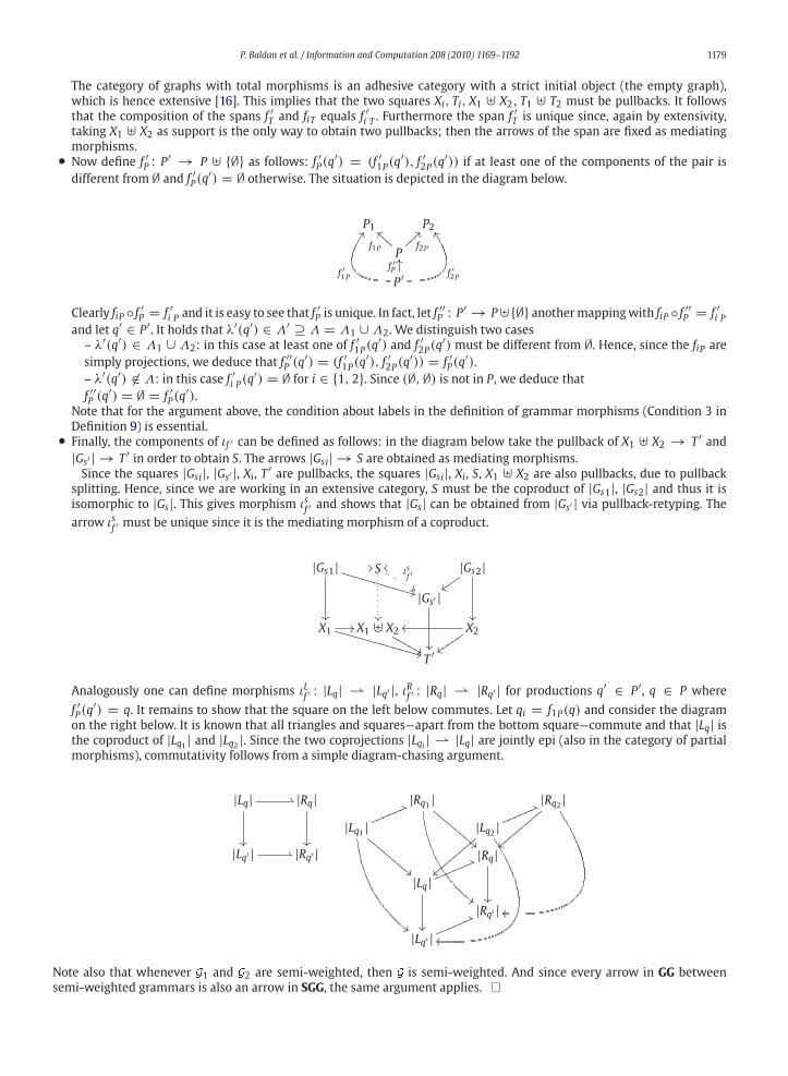
P. Baldan et al. / Information and Computation 208 (2010) 1169–1192 1179
The category of graphs with total morphisms is an adhesive category with a strict initial object (the empty graph),
which is hence extensive [16]. This implies that the two squares Xi, Ti, X1 � X2, T1 � T2 must be pullbacks. It follows
that the composition of the spans f ′T and fiT equals f ′i T . Furthermore the span f ′T is unique since, again by extensivity,
taking X1 � X2 as support is the only way to obtain two pullbacks; then the arrows of the span are fixed as mediating
morphisms.• Now define f ′P : P′ → P � {∅} as follows: f ′P(q′) = (f ′1P(q′), f ′2P(q′)) if at least one of the components of the pair is
different from ∅ and f ′P(q′) = ∅ otherwise. The situation is depicted in the diagram below.
P1 P2
Pf1P
�����f2P
�����
P′f ′1P
��
f ′2P
f ′P
Clearly fiP ◦ f ′P = f ′i P and it is easy to see that f ′P is unique. In fact, let f ′′P : P′ → P�{∅} anothermappingwith fiP ◦ f ′′P = f ′i Pand let q′ ∈ P′. It holds that λ′(q′) ∈ Λ′ ⊇ Λ = Λ1 ∪ Λ2. We distinguish two cases
– λ′(q′) ∈ Λ1 ∪ Λ2: in this case at least one of f ′1P(q′) and f ′2P(q′) must be different from ∅. Hence, since the fiP are
simply projections, we deduce that f ′′P (q′) = (f ′1P(q′), f ′2P(q′)) = f ′P(q′).– λ′(q′) �∈ Λ: in this case f ′i P(q′) = ∅ for i ∈ {1, 2}. Since (∅, ∅) is not in P, we deduce that
f ′′P (q′) = ∅ = f ′P(q′).Note that for the argument above, the condition about labels in the definition of grammar morphisms (Condition 3 in
Definition 9) is essential.• Finally, the components of ιf ′ can be defined as follows: in the diagram below take the pullback of X1 � X2 → T ′ and
|Gs′ | → T ′ in order to obtain S. The arrows |Gsi| → S are obtained as mediating morphisms.
Since the squares |Gsi|, |Gs′ |, Xi, T′ are pullbacks, the squares |Gsi|, Xi, S, X1 � X2 are also pullbacks, due to pullback
splitting. Hence, since we are working in an extensive category, S must be the coproduct of |Gs1|, |Gs2| and thus it is
isomorphic to |Gs|. This gives morphism ιsf ′ and shows that |Gs| can be obtained from |Gs′ | via pullback-retyping. The
arrow ιsf ′ must be unique since it is the mediating morphism of a coproduct.
|Gs1|
��
�� �� S ιsf ′��
��
|Gs2|
��
����
|Gs′ |
��
X1��
�� X1 � X2
������� X2��
�������
T ′
Analogously one can define morphisms ιLf ′ : |Lq| ⇀ |Lq′ |, ιR
f ′ : |Rq| ⇀ |Rq′ | for productions q′ ∈ P′, q ∈ P where
f ′P(q′) = q. It remains to show that the square on the left below commutes. Let qi = f1P(q) and consider the diagram
on the right below. It is known that all triangles and squares—apart from the bottom square—commute and that |Lq| isthe coproduct of |Lq1 | and |Lq2 |. Since the two coprojections |Lqi | ⇀ |Lq| are jointly epi (also in the category of partial
morphisms), commutativity follows from a simple diagram-chasing argument.
|Lq| �
��
|Rq|
��|Lq′ | � |Rq′ |
|Rq1 |
��
��
|Rq2 |
������
����
��
|Lq1 |
��
�������
��
|Lq2 |�������
������
����
��
|Rq|
��
|Lq|
��
�������
|Rq′ ||Lq′ |
�������
Note also that whenever �1 and �2 are semi-weighted, then � is semi-weighted. And since every arrow in GG between
semi-weighted grammars is also an arrow in SGG, the same argument applies. �

1180 P. Baldan et al. / Information and Computation 208 (2010) 1169–1192
2.3. Occurrence grammars and unfolding
A grammar � is safe if (i) for all H such that Gs ⇒∗ H, H is injective, and (ii) for each q ∈ P, the left- and right-hand side
graphs Lq and Rq are injective.
In words, in a safe grammar each graph G reachable from the start graph is injectively typed, and thus we can identify it
with the corresponding subgraph tG(|G|) of the type graph. With this identification, a production can only be applied to the
subgraph of the type graph which is the image via the typing morphism of its left-hand side. Thus, according to its typing,
we can think that a production produces, preserves or consumes items of the type graph, and using a net-like language, we
speak of pre-set, context and post-set of a production, correspondingly. Intuitively the type graph T plays the role of the set
of places of a net, whereas the productions in P correspond to the transitions.
Definition 11 (Pre-set, post-set and context of a production). Let � be a graph grammar. For any production q ∈ P we define
its pre-set •q, context q and post-set q• as the following subsets of ET ∪ NT :
•q = tLq (|Lq| − |dom(rq)|) q = tLq (|dom(rq)|) q• = tRq (|Rq| − rq(|dom(rq)|)).Symmetrically, for each item x ∈ T we define •x = {q ∈ P | x ∈ q•}, x• = {q ∈ P | x ∈ •q}, x = {q ∈ P | x ∈ q}.
Causal dependencies between productions are captured as follows.
Definition 12 (Causality). The causality relation of a grammar � is the (least) transitive relation < over Elem(�) satisfying,for any node or edge x ∈ T , and for productions q, q′ ∈ P,
1. if x ∈ •q then x < q;
2. if x ∈ q• then q < x;
3. if q• ∩ q′ �= ∅ then q < q′.
As usual ≤ is the reflexive closure of <. Moreover, for x ∈ Elem(�) we denote by �x� the set of causes of x in P, namely
{q ∈ P | q ≤ x}.As it happens in Petri nets with read arcs, the fact that a production application not only consumes and produces, but also
preserves a part of the state, leads to a form of asymmetric conflict between productions; for a more thorough discussion of
asymmetric event structures see A.1 and [17].
Definition 13 (Asymmetric conflict). The asymmetric conflict relation of a grammar � is the binary relation ↗ over the set of
productions, defined by:
1. if q ∩ •q′ �= ∅ then q ↗ q′;2. if •q ∩ •q′ �= ∅ and q �= q′ then q ↗ q′;3. if q < q′ then q ↗ q′.
Intuitively, whenever q ↗ q′, q can never follow q′ in a computation. This holds when q preserves something deleted
by q′ (Condition 1), trivially when q and q′ are in conflict (Condition 2) and also when q < q′ (Condition 3). Conflicts are
represented by cycles of asymmetric conflict: if q1 ↗ q2 ↗ . . . ↗ qn ↗ q1 then the entire set {q1, . . . , qn} will never
appear in the same computation.
An occurrence grammar is an acyclic grammar which represents, in a branching structure, several possible computations
beginning from its start graph and using each production at most once. Recall that a relation R ⊆ X × X is called finitary if
for any x ∈ X , the set {y ∈ X | R(y, x)} is finite.Definition 14 (Occurrence grammar). An occurrence grammar is a safe grammar � = 〈T, Gs, P, π, Λ, λ〉 such that
1. causality< is irreflexive, its reflexive closure≤ is a partial order, and, for any q ∈ P, the set �q� is finite and asymmetric
conflict ↗ is acyclic on �q�;2. any item x in T is created by at most one production in P, i.e., |•x| ≤ 1;
3. the start graph Gs is the setMin(�) of minimal elements of 〈Elem(�), ≤〉 (with the graphical structure inherited from
T and typed by the inclusion).
A finite occurrence grammar is deterministic if relation↗+, the transitive closure of↗, is irreflexive. We denote byOGG the
full subcategory of GGwith occurrence grammars as objects.
Intuitively, by Condition 1 the causes of any event are finite and free of conflicts (cycles of asymmetric conflict), while
Condition 2 ensures that any item is generated atmost once in a computation. ByCondition 3, the start graphof an occurrence

P. Baldan et al. / Information and Computation 208 (2010) 1169–1192 1181
grammar is determined by Min(�). An occurrence grammar is deterministic when it does not contain conflicts so that all
its productions can be executed in the same computation. Given two occurrence grammars �1 and �2, we say that �1 is a
sub-grammar of �2, if �1 ⊆ �2, componentwise, and the inclusion of �1 into �2 is a grammar morphism. In the sequel, the
productions of an occurrence grammar will often be called events.
The notion of configuration captures the intuitive idea of (deterministic) computation in an occurrence grammar.
Definition 15 (Configuration). Let � be an occurrence grammar. A configuration is a subset C ⊆ P satisfying the following
requirements:
1. for any q ∈ C it holds that �q� ⊆ C;
2. ↗C , the asymmetric conflict restricted to C, is acyclic and finitary.
The set of configurations of � is denoted as Conf (�).
It is shown in [10] that, indeed, configurations faithfully represent computations in an occurrence grammar: all the
productions in a configuration can be applied in a derivation exactly once in any order compatible with ↗, and all and only
the derivations in � can be obtained in this way. Hence the runs of an occurrence grammar are exactly the linearisations,
compatible with the asymmetric conflict relation, of its configurations, i.e., the following holds:
Proposition 2 (Configurations as runs). Let � be an occurrence grammar. Then Runs(�) = {q1 . . . qn | {q1, . . . , qn} ∈Conf (�) ∧ ∀i < j. ¬(qj ↗ qi)}.
Since occurrence grammars are particular semi-weighted grammars, there is an inclusion functor � : OGG → SGG. As
an easy corollary of [10, Theorem 45], this functor has a right adjoint. We remark that this theorem would not hold if we
considered GG instead of SGG.
Theorem 1 (Coreflection). The inclusion functor � : OGG → SGG has a right adjoint, the so-called unfolding functor
� : SGG → OGG.
As a consequence of the above result �, as a right adjoint, preserves all limits and in particular products, i.e., given two
grammars �1 and �2, it holds that �(�1 × �2) = �(�1) × �(�2).The result in [10] is obtained through the explicit definition of the unfolding �(�). Given a grammar � the unfolding
construction produces an occurrence grammar which fully describes its behaviour recording all the possible graph items
which are generated and the occurrences of productions. The unfolding of � is constructed inductively by starting from a
grammar which only includes the start graph of � (which is also used as a type graph), and then extending such grammar,
at any step, by applying productions in any possible way to the type graph, without deleting items but only generating
new ones, and recording the corresponding production instances. The result is an occurrence grammar �(�) and a grammar
morphism f : �(�) → �, called the folding morphism, which maps each item (instance of production or graph item) of the
unfolding to the corresponding item of the original grammar. The construction is not formally defined here, we refer the
reader to [10]. In Section 4 we will show an example of an unfolding.
As an immediate consequence of the fact that the unfolding �(�) completely captures the behaviour of a grammar �, we
have the following result.
Proposition 3 (Completeness of the unfolding). For any semi-weighted graph grammar � it holds that
λ∗(Runs(�(�))) = λ∗(Runs(�)).
3. Interleaving structures
Interleaving structures [18] are a semanticmodelwhich captures the behaviour of a systemas the collection of its possible
runs. They are used as a simpler intermediate model which helps in stating and proving the correctness of the diagnosis
procedure.
An interleaving structure is essentially a collection of runs (sequences of events) satisfying suitable closure properties.
Given a set E, we will denote by E� the set of sequences over E in which each element of E occurs at most once.
Definition 16 (Interleaving structures). A (labelled) interleaving structure is a tuple � = (E, R, Λ, λ)where E is a set of events,
λ : E → Λ is a labelling of events and R ⊆ E� is the set of runs, satisfying: (i) R is prefix-closed, (ii) R contains the empty
run ε, and (iii) every event e ∈ E occurs in at least one run.
The components of an interleaving structure � will be denoted by E, R, Λ, λ, possibly with subscripts. The category
of interleaving structures, as defined below, is adapted from [18] by changing the notion of morphisms in order to take

1182 P. Baldan et al. / Information and Computation 208 (2010) 1169–1192
into account the labels. This is needed to obtain a product which expresses a suitable form of synchronised
composition.
Definition 17 (Interleaving morphisms). Let �i with i ∈ {1, 2} be interleaving structures. An interleaving morphism from �1
to �2 is a partial function θ : E1 ⇀ E2 on events such that
1. Λ2 ⊆ Λ1;
2. for each e1 ∈ E1, θ(e1)↓ iff λ1(e1) ∈ Λ2 and, in this case, λ2(θ(e1)) = λ1(e1);3. for every r ∈ R1 it holds that θ∗(r) ∈ R2.
Morphism θ is called a projection if it is surjective on runs, i.e., θ∗ : R1 → R2 is surjective. The category of interleaving
structures and morphisms is denoted Ilv.
Observe that an interleaving morphism θ : �1 → �2 is necessarily injective on the events occurring in each run, i.e., for
any run r1 = e1 . . . ek ∈ R1, for i �= j we have θ(ei) �= θ(ej), when both are defined. Otherwise, θ(r) could not be a run in
�2 as it would contain two occurrences of the same event.
An occurrence grammar can be easily mapped to an interleaving structure, by simply taking all the runs of the grammar.
Definition 18 (Interleaving structures for occurrence grammars). For an occurrence grammar � we define
Ilv(�) = (P, Runs(�), Λ, λ).
We next characterise the categorical product in Ilv, which turns out to be, as in GG, the desired form of synchronised
product.
Proposition 4 (Product of interleaving structures). Let �1 and �2 be two interleaving structures. Then the product object �1�2
is the interleaving structure � = (E, R, Λ, λ) defined as follows. Let
E′ = {(e1, e2) | e1 ∈ E1, e2 ∈ E2, λ1(e1) = λ2(e2)}∪ {(e1, ∗) | e1 ∈ E1, λ1(e1) �∈ Λ2} ∪ {(∗, e2) | e2 ∈ E2, λ2(e2) �∈ Λ1}
and let πi : E ⇀ Ei be the obvious partial projections (e.g., π1(e1, x2) = e1 and π1(∗, x2) ↑ for e1 ∈ E1 and x2 ∈ E2 ∪ {∗}).Then R = {r ∈ (E′)� | π∗
1 (r) ∈ R1, π∗2 (r) ∈ R2}, E = {e′ ∈ E′ | e occurs in some run r ∈ R}, Λ = Λ1 ∪ Λ2 and λ is defined
in the obvious way.
Proof. Let �′ be any interleaving structure and let θi : �′ → �i be morphisms. Let us define θ : �′ → � as follows:
θ(e′) ↑ if θ1(e′)↑ and θ2(e
′)↑
θ(e′) =
⎧⎪⎪⎪⎪⎨⎪⎪⎪⎪⎩
(θ1(e′), θ2(e′)) if θ1(e
′)↓ and θ2(e′)↓
(θ1(e′), ∗) if θ1(e
′)↓ and θ2(e′)↑
(∗, θ2(e′)) if θ1(e
′)↑ and θ2(e′)↓
Trivially, the diagram, seen in the category of sets and partial functions, commutes and θ is uniquely determined.
Hence to conclude we just need to show that θ is a well-defined interleaving morphism. In fact,
1. Since there are morphisms θi : �′ → �i, necessarily Λi ⊆ Λ′, for i ∈ {1, 2} and thus Λ = Λ1 ∪ Λ2 ⊆ Λ′.2. For each e′ ∈ E′, θ(e′)↓ iff λ′(e′) ∈ Λ. In more detail:
θ(e′)↓ ⇐⇒ θ1(e′)↓ or θ2(e
′)↓⇐⇒ λ′(e′) ∈ Λ1 or λ′(e′) ∈ Λ2
⇐⇒ λ′(e′) ∈ Λ1 ∪ Λ2 = Λ.
And clearly, when defined, λ′(e′) = λ(θ(e′))3. For any r′ ∈ R′, θ∗(r′) ∈ R. In fact, notice that, due to commutativity, π∗
i (θ∗(r′)) = θ∗i (r′) ∈ Ri. Hence, by
construction, θ∗(r′) ∈ R. �
4. Diagnosis and pruning
In this section, we use the tools introduced so far in order to formalise the diagnosis problem. Then we show how,
given a graph grammar model and an observation for such a grammar, the diagnosis can be obtained by first taking the

P. Baldan et al. / Information and Computation 208 (2010) 1169–1192 1183
product of the model and the observation, considering its unfolding and finally pruning such unfolding in order to remove
incomplete explanations. As alreadymentioned, typically only a subset of the productions in the system is observable. Hence,
for this section, we fix a graph grammar � with Λ as the set of labels, and a subset Λ′ ⊆ Λ of observable labels; an event
or production is called observable if it has an observable label. In order to keep explanations finite, we will only consider
systems that satisfy the following observability assumption (compare [2,19]): any infinite run must contain an infinite number
of observable productions.
In the sequel we will need to consider the runs of a system which have a number of observable events coinciding with
the number of events in the observation. For this aim the following definition will be useful.
Definition 19 (n-Runs of a grammar). Let � be a graph grammar. For a given n ∈ N we denote by Runsn(�) the set of all runs
for which the number of observable productions equals n.
The outcome of the diagnosis procedure is an occurrence grammar which, intuitively, collects all the behaviours of the
grammar �modelling the system, which are able to “explain” the observation.
An observation can be a sequence (in the case of a single observer) or a set of sequences (in the case ofmultiple distributed
observers) of alarms (observable events). Here we consider, more generally, partially ordered sets of observations, which
can be conveniently modelled as deterministic occurrence grammars.
Definition 20 (Observation grammar). An observation grammar � for a given grammar �, with observable labels Λ′, is a
(finite) deterministic occurrence grammar labelled over Λ′.
Given a sequence of observed events, we can easily construct an observation grammar� having that sequence as observ-
able behaviour. It will have a production for each event in the sequence, with the corresponding label. Each such production
consumes a resource generated by the previous one in the sequence (or an initial resource in the case of the first production).
The same construction applies to general partially ordered sets of observations.
Example 3. In the running example grammar � (see Figs. 9 and 10), assume that we have the following observation:
snd cnode cconn2 crcv, i.e., we observe, in sequence, the sending of a message, the creation of a new intermediary node
with the corresponding connection, the creation of a connection to a receiver and the reception of a corrupted message. As
explained above, these four observations can be represented by a simple grammar � (see Fig. 13) with four productions,
each of which either consumes an initial resource or a resource produced by the previous production. These resources are
modelled as 0-ary edges (labelled X , Y ,W , Z). The start graph is depicted with bold lines, and the left- and right-hand sides
of the productions of the occurrence grammar are indicated by using a Petri-net-like notation: productions are drawn with
black rectangles connected to the edges they consume or produce by dashed lines.
When unfolding the product of a grammar � with its observation �, we obtain a grammar � = �(� × �) with a
morphismπ : � → �, arising as the image through the unfolding functor of the projection �×� → � (since the unfolding
of an occurrence grammar is the grammar itself). Now, as grammar morphisms are simulations [10], given the morphism
π : � → � we know that any configuration in � is mapped to a configuration in �. Say that a configuration in � is a full
explanation of� if it is mapped to the configuration of� including all its productions. As � can still contain events belonging
only to incomplete explanations, the aim of pruning is to remove such events.
Definition 21 (Pruning). Let π : � → � be a grammarmorphism from an occurrence grammar � to an observation�. Then,
the pruning of π , denoted by Pr(π), is the sub-grammar of � obtained by keeping only the productions in
{q ∈ �� | ∃C ∈ Conf (�) : (q ∈ C ∧ π(C) = ��)}.The next technical lemma shows that applying the pruning operation to a morphism π : � → � no runs in � which
provide a full explanation of � are lost.
Lemma 1 (Interleavings of a pruned grammar). Let π : � → � be a grammar morphism from an occurrence grammar to an
observation � with n productions. Then
Runsn(Pr(π)) = {r ∈ Runs(�) | π∗(r) ∈ Runsn(�)}.
Fig. 13. A graph grammar representing an observation�, given in a Petri-net-like notation.

1184 P. Baldan et al. / Information and Computation 208 (2010) 1169–1192
Proof. We first show that Runsn(Pr(π)) ⊆ {r ∈ Runs(�) | π∗(r) ∈ Runsn(�)}. Take any run r ∈ Runsn(Pr(π)). Thenclearly r ∈ Runs(�) since Pr(π) is a sub-grammar of �. Furthermore, since π preserves the observable productions, π∗(r)must contain exactly n observable productions and thus it belongs to Runsn(�).
For the other direction take any run r ∈ Runs(�) such that π∗(r) ∈ Runsn(�). Then, again, r must contain exactly n
observable productions. Furthermore take the configuration C consisting of the productions in r. Since π maps C to the set
of all productions of �, none of the productions of r is removed during the pruning phase. Hence r ∈ Runsn(Pr(π)). �
Discussing the efficiency of pruning algorithms is outside the scope of the paper; for sequential observations an on-the-fly
algorithm is discussed in [5].
As described above, the diagnosis is constructed by first taking the product of � with the observation (this intuitively
represents the system constrained by the observation). This product is then unfolded to get an explicit representation of the
possible behaviours explaining the observation. Finally, a pruning phase removes from the resulting occurrence grammar
the events belonging (only) to incomplete explanations. This is formalised in the definition below.
Definition 22 (Diagnosis grammar). Let � be the grammarmodelling the system of interest and let� be an observation. Take
the product � × �, the right projection ϕ : � × � → � and consider π = �(ϕ) : �(� × �) → �. Then the occurrence
grammar Pr(π) is called the diagnosis grammar for the model � and the observation �, and it is denoted by D(�,�).
Since the observability assumption holds, it can be shown that the diagnosis grammar is finite whenever the observation
is finite. Roughly, the argument is as follows. Assume that the diagnosis grammar is infinite. Since it is finitely branching
it must contain an infinite computation, which, by the observability assumption, would contain infinitely many observable
events. However, this cannot be the case since all computations in thediagnosis grammar contain atmost asmanyobservable
events as the observation.
Example 4. We can compute the product of grammars� and � and unfold it. For the sake of clarity Fig. 14 shows only a
prefix of the unfolding. (The full unfolding is presented in Section 6.) In order to give a compact representation of such prefix
we again use a Petri-net-like notation. Edges that are preserved by a production are indicated by read arcs, i.e., dashed arcs
without arrowhead that connect an edge and a black rectangle.
The considered prefixdepicts one possible explanation: here themessage is sent (event a) and crosses the first connection
(b). Possibly concurrently a new intermediate node and a connection to this node is created (c). The new node is initially
inactive and it becomes active immediately after (d). The new connection is crossed by the message (e) and, in a possibly
concurrent step, a new connection to the receiver is created (f). Such connection is corrupted (g), leading to the corruption
of the message (h) and its reception by the receiver (i). Observable events are indicated by bold face letters.
Fig. 14. Running example: prefix of the unfolding of the product.

P. Baldan et al. / Information and Computation 208 (2010) 1169–1192 1185
Several events of the unfolding have been left out due to space constraints, for instance:
• Events belonging to alternative explanations: the corruption of the first connection or the corruption of the newly created
middle connection (or the corruption of any non-empty subset of these connections). Alternatively it might have been
the case that the new connection was created from the original intermediate node directly to the receiver.• Events that are not directly related to the failure, such as the corruption of the first or second connection after themessage
has crossed.
Furthermore there are events belonging to prefixes of the unfolding that cannot be extended to a full observation. For
instance, the full unfolding would contain an event corresponding to an (uncorrupted) message crossing the rightmost
uncorrupted connection C. However, this is a false trail since, after this, it would be impossible to complete the explanation
with the reception of a corrupted message (in fact, this would require the sending of a newmessage, an event which would
be visible and inconsistentwith the observation). These events belonging only to incomplete explanations are removed from
the unfolding in the pruning phase.
We remark that—due to the presence of concurrent events—the unfolding is a much more compact representation of
everything that might have happened in the system than the set of all possible interleavings of events.
5. Correctness of the diagnosis
Wenowshowourmain result, stating that the runs of the diagnosis grammarproperly capture all those runs of the system
modelwhichexplain theobservation. This is donebyexploiting the coreflection result (Theorem1) andbyadditionally taking
care of the pruning phase (Definition 21).
To lighten the notation, hereafter, given an interleaving structure � we write λ∗(I) for λ∗(RI). Recall that, given
f : Λ1 ⇀ Λ2, we denote by f ∗ : Λ∗1 → Λ∗
2 the (non-strict) extension of f to sequences. Then f−1 : �(Λ∗2) → �(Λ∗
1) is itsinverse.
A first lemma shows that the labelled runs of a product of occurrence grammars �1 × �2 can be obtained by suitably
combining pairs of compatible runs of�1 and�2. By “compatible” wemean that they admit a common extension, obtained
by interleaving the run of �1 with events labelled in (Λ1 ∪ Λ2) − Λ2 and, dually, the run of �2 with events labelled in
(Λ1 ∪ Λ2) − Λ1.
Lemma 2. Let �1, �2 be two occurrence grammars and let fi : Λ1 ∪ Λ2 ⇀ Λi (i ∈ {1, 2}) be the obvious partial inclusions.
Then it holds that
λ∗ (Ilv (�1 × �2)) = f−11
(λ∗1 (Ilv(�1))
) ∩ f−12
(λ∗2 (Ilv(�2))
).
Proof. Let �1 = Ilv(�1), �2 = Ilv(�2) and � = �1 × �2 = Ilv(�1) × Ilv(�2). Furthermore let πi : � → �i, i ∈ {1, 2} be the
projections. We first observe that
λ∗(�) = λ∗(R�) ={λ∗�(r) | r ∈ (E�)
� ∧ π∗1 (r) ∈ R1 ∧ π∗
2 (r) ∈ R2
}
(†)= {w ∈ Λ∗ | f ∗1 (w) ∈ λ∗
1(R1), f∗2 (w) ∈ λ∗
2(R2)}
= f−11
(λ∗1(R1)
) ∩ f−12
(λ∗2(R2)
)
= f−11
(λ∗1(�1)
) ∩ f−12
(λ∗2(�2)
).
The equality marked (†) above, which is not obvious, can be shown as follows.
⊆: Take r ∈ R� and consider the sequence of labels λ∗�(r) associated with r. Since π1 is defined exactly on the events
whose label is in Λ1, it holds that λ∗1(π
∗1 (r)) = f ∗1 (λ∗
�(r)), hence f ∗1 (λ∗
�(r)) ∈ λ∗
1(R1). Similarly one can show that
f ∗2 (λ∗�(r)) ∈ λ∗
2(R2).
⊇: Let w ∈ Λ∗ be such that f ∗1 (w) ∈ λ∗1(R1) and f ∗2 (w) ∈ λ∗
2(R2). Assume that w = c1 . . . ck , f∗1 (w) = ci1 . . . cin and
f ∗2 (w) = cj1 . . . cjm . Furthermore let r1 = fi1 . . . fin ∈ R1 be a run with λ∗1(r1) = f ∗1 (w) and let r2 = gj1 . . . gjm ∈ R2
be a run with λ∗2(r2) = f ∗2 (w). Now construct a run r = e1 . . . en with
ei =
⎧⎪⎪⎪⎨⎪⎪⎪⎩
(fi, gi) if ci ∈ Λ1 ∩ Λ2
(fi, ∗) if ci ∈ Λ1\Λ2
(∗, gi) if ci ∈ Λ2\Λ1
.
It holds that π∗1 (r) = r1, π
∗2 (r) = r2 and obviously λ∗
I (r) = w. Hence w is contained in the left-hand set.

1186 P. Baldan et al. / Information and Computation 208 (2010) 1169–1192
Wenext show thatλ∗(�) = λ∗(Ilv(�1×�2)), and thuswe conclude. This follows from Lemma 3 in A.2which guarantees
the existence of a total projection δ : Ilv(�1 × �2) → �. In fact, since δ respects labellings and is total, whenever it maps
two runs of Ilv(�1 �2) to one run of �, they must be associated with the same label sequence. Using, additionally, the fact
that δ is surjective on runs, the desired equality immediately follows. �
The next proposition shows that considering the product of the original grammar � and of the observation �, taking its
unfolding and the corresponding labelled runs, we obtain exactly the runs of � compatible with the observation.
Proposition 5. Let � be a grammar and � an observation, where Λ is the set of labels of � and Λ′ ⊆ Λ the set of labels of �.
Furthermore let f : Λ ⇀ Λ′ be the obvious partial inclusion. Then it holds that:
λ∗ (Ilv(�(�× �))) = λ∗ (Runs(�)) ∩ f−1 (λ∗(Runs(�))
).
Proof. First, recall that, by Proposition 3, λ∗(Runs(�)) = λ∗(Ilv(�(�))) and λ∗(Runs(�)) = λ∗(Ilv(�(�))) = λ∗(Ilv(�)).Furthermore due to the fact that unfolding is a coreflection (Theorem 1), we have �(�× �) = �(�) × �(�).
Hence we have to show that
λ∗(Ilv((�(�)) × (�(�)))) = λ∗(Ilv(�(�))) ∩ f−1(λ∗(Ilv(�(�)))).
This is a corollary of Lemma 2 for �1 = �(�), �2 = �(�) = �, Λ1 = Λ, Λ2 = Λ′; furthermore f corresponds to f2 and f1is the identity since Λ′ ⊆ Λ. �
We can finally prove that the described diagnosis procedure is complete, i.e., given an observation of size n, the runs of
the diagnosis grammar D(�,�) with n observable events are in 1–1-correspondence with those runs of � that provide a full
explanation of the observation. As a preliminary result, on the basis of Proposition 5, one could have shown that the same
holds replacing the diagnosis grammar with �(� × �), i.e., the unpruned unfolding. The result below additionally shows
that no valid explanation is lost during the pruning phase.
Theorem 2 (Correctness of the diagnosis). With the notation of Proposition 5 it holds that:
λ∗(Runsn(D(�,�))) = λ∗(Runs(�)) ∩ f−1(λ∗(Runsn(�))).
That is, the maximal interleavings of the diagnosis grammar (seen as label sequences) are exactly the runs of the model which
explain the full observation.
Proof. By definition
λ∗(Runsn(D(�,�))) = λ∗(Runsn(Pr(π2))), (1)
where, if we let � = �(� × �), then π2 : � → � is the (image through the unfolding functor of the) second projection of
the product. By Lemma 1, the set (1) is the same as
λ∗ ({r ∈ Runs(�) | π∗(r) ∈ Runsn(�)
}). (2)
We will now show that set (2) coincides with
λ∗(Runs(�)) ∩ f−1(λ∗(Runsn(�))). (3)
⊆: Let w = λ∗(r) for some r ∈ Runs(�) and π∗(r) ∈ Runsn(�). By Proposition 3, w ∈ λ∗(Runs(�)). The fact that
w ∈ f−1(λ∗(Runsn(�))) easily follows by observing that λ∗(π∗2 (r)) ∈ λ∗(Runsn(�)) is a subsequence of w where
all unobservable labels are missing and these labels, by definition, can be reinserted by f−1. This proves the inclusion
(2) ⊆ (3).
⊇: Let w ∈ λ∗(Runs(�)) ∩ f−1(λ∗(Runsn(�))). Observe that
λ∗ (Runs(�)) ∩ f−1 (λ∗(Runsn(�))
)
⊆ λ∗ (Runs(�)) ∩ f−1 (λ∗(Runs(�))
)
= λ∗ (Ilv(�)) (Proposition 5).
Hence there exists a run r ∈ Runs(�) such that λ∗(r) = w. By definition of a morphism, π∗2 (r) ∈ Runs(�) and
λ∗(π∗2 (r)) = f ∗(λ∗(r)) = f ∗(w) ∈ λ∗(Runsn(�)) (by choice of w). Hence also π∗
2 (r) ∈ Runsn(�).
Summingup r ∈ {r ∈ Runs(�) | π2(r) ∈ Runsn(�)}andsinceλ∗(r) = wweconcludew ∈ λ∗(π−12 (Runsn(�))). �

P. Baldan et al. / Information and Computation 208 (2010) 1169–1192 1187
Fig. 15. Spurious runs in a diagnosis grammar.
Observe that, due to the non-deterministic nature of the diagnosis grammar, events which are kept in the pruning phase
as they are part of some full explanation of the observation, can also occur in a different configuration. As a consequence,
although all inessential events have been removed, the diagnosis grammar can still contain spurious configurations which
cannot be extended to full explanations. As an example, consider the graph grammar � in Fig. 15, given in a Petri-net-like
notation. Assume we observe three unordered events a, b, c. Then the unfolding of the product basically corresponds to �
itself. In the pruning phase nothing is removed, since each event is part of a chain consisting of a, b, c which fully explains
the observation. However, since different explanations can interfere, there is a configuration (indicated by the dashed closed
line) that cannot be further extended to an explanation.
Fig. 16. Type graph of the unfolding of the product.
1188 P. Baldan et al. / Information and Computation 208 (2010) 1169–1192
6. Experimental evaluation
In order to give an idea about the practical applicability of our approach, we use some existing tools in order to compare
the size of the unfolding with that of interleaving-based models which could be used for analysing the running example
(message passing over a network).
Graph grammars are unfolded by using an extension of the tool Augur [20], whose original purpose is to compute ap-
proximated unfoldings in order to abstract infinite-state graph transformation systems. The extension, under the assumption
that rules do not delete nodes, can also be used to produce an ordinary, non-approximated, unfolding of a graph grammar. In
our running example this assumption is violated only by rule fail, which is however not involved in the specific observation
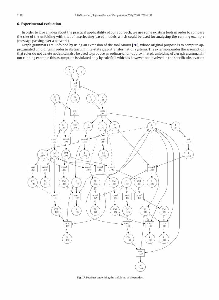
Fig. 17. Petri net underlying the unfolding of the product.

P. Baldan et al. / Information and Computation 208 (2010) 1169–1192 1189
that we are considering and thus can be safely omitted. We have not yet implemented the computation of the product of
two graph grammars (this is done manually) and pruning.
We took the running example grammar � (see Figs. 9 and 10) and computed the product of this grammar and the
observation grammar for the sequence snd cnode cconn2 crcv. The unfolding is shown in Figs. 16 and 17, visualised by using
GraphViz. 1 For reasons of clarity the output of the tool, i.e., the unfolding, is split into two components: the underlying type
graph and a Petri netwhich represents the rules, depicting deletion, preservation and creation of the edges of the type graph.
The unfolding includes 40 edges, 4 nodes and 26 transitions (a prefix of this unfoldingwas already presented in Figure 14).
The unfolding shown here is still unpruned. In the pruned version the transitions labelled cross1_115 and cross1_129would be removed. They correspond to cases where an uncorrupted message arrives at the receiver, thus making the last
observation (crcv) impossible.
The five transitions labelled crcv represent five distinct situations: either the message has passed from the sender to
the original intermediate node cirectly to the receiver and the corruption of the message has been caused by the first
connection (crcv_127) or by the second connection (crcv_139). Or themessage has passed from the sender to the original
intermediate node to a new intermediate node to the receiver and its corruption has been caused by the first (crcv_143),second (crcv_141) or third (crcv_147) connection. Note that the last event (crcv_147) corresponds to event i in Figure 14.
In order to get an idea of the cost of a diagnosis algorithm based on interleavings, we can compute the product of the
transition system of� with an automaton representing the observation. The size of the resulting transition system is the
same as the size of the state space of the product grammar.We determined the corresponding number of states (taken up to
isomorphisms)byusingGroove, 2 a tool for state spaceexplorationandmodel-checkingofgraphtransformationsystems [21].
The state space consists of 205 states and it is not straightforward to deduce manually the diagnosis information from the
corresponding transition system.
Since this example is still fairly smallwe took the samegrammar�andconsidereda slightly longerobservation sequence:
snd cnode cconn2 cnode crcv. In this case, the unfolding consists of 83 edges, 8 vertices and 57 transitions, whereas the
state space contains 1338 states. In general, for highly concurrent systems, the unfolding tends to be exponentially smaller
than the interleaving model; this blow up in the size will decrease for systems where the degree of concurrency is limited.
7. Conclusion
In thispaper,we formalisedevent-baseddiagnosis for systemswithvariable topologies,modelledasgraph transformation
systems. In particular we have shown how to exploit the coreflection result for the unfolding of graph grammars in order to
show the correctness of a diagnosis procedure generating partially ordered explanations for a given observation.
We are confident that the approach presented in the paper, although developed for transformation systems over hyper-
graphs, canbegeneralised to themoreabstract settingofadhesivecategories. Inparticularwehavedevelopedageneralisation
of the unfolding procedure [22] that works for spo-rewriting in (suitable variations of) adhesive categories [16]. This would
allow one to have a kind of parametric framework which can be used to instantiate the results of this paper to more general
rewriting theories, e.g., rewriting graphs with scopes, graphs with second-order edges, and other kind of graph structures
(which for instance occur in the various UML diagrams).
We are also interested in distributed diagnosis where every observer separately computes possible explanations of local
observations that however have to be synchronised. In [18] we already considered distributed unfolding of Petri nets; for
diagnosis however, the non-trivial interaction of distribution and pruning has to be taken into account. Distribution will
require the use of pullbacks of graph morphisms, in addition to products. Pullbacks are needed since we want to describe
system composition via a common interface.
Acknowledgments
We are very grateful to the anonymous referees for their valuable comments on the preliminary version of the paper.
Appendix A. Auxiliary material
In this appendix, we first briefly recap the functorial event structure semantics for graph transformation systems, as
defined in [10] and adapt them to the labelled setting. The semantics is given in terms of asymmetric event structures
(aes’s) [17], a generalisation of prime event structures where the conflict relation is allowed to be non-symmetric. A functor
mapping any occurrence grammar into an aes is defined. The event structure semantics of a graph grammar is obtained by
taking the aes associated to the unfolding of the grammar.
Then, using the characterisation of the aes’s semantics as a right adjoint,weprove aproperty of the product of interleaving
structures which is fundamental for the theory in the paper.
1 http://www.graphviz.org/2 http://groove.cs.utwente.nl/groove-home/

1190 P. Baldan et al. / Information and Computation 208 (2010) 1169–1192
A.1. From occurrence grammars to asymmetric event structures
For technical reasons we first introduce pre-asymmetric event structures. Then asymmetric event structures will be
defined as special pre-asymmetric event structures satisfying a suitable condition of “saturation”.
Definition 23 (Asymmetric event structure). Apre-asymmetric event structure (pre-aes) is a tuple� = 〈E, ≤, ↗, Λ, λ〉, where
E is a set of events, ≤, ↗ are binary relations on E called causality and asymmetric conflict, respectively, and λ : P → Λ is a
labelling over the set of labels Λ, such that:
1. causality ≤ is a partial order and �e� = {e′ ∈ E | e′ ≤ e} is finite for all e ∈ E;
2. asymmetric conflict ↗ satisfies, for all e, e′ ∈ E:
(a) e < e′ ⇒ e ↗ e′,(b) ↗ is acyclic in �e�, where, as usual, e < e′ means e ≤ e′ and e �= e′.
An asymmetric event structure (aes) is a pre-aeswhich additionally satisfies:
3. for any e, e′ ∈ E, if ↗ is cyclic in �e� ∪ �e′� then e ↗ e′ (and also e′ ↗ e).
Conditions1and2areeasilyunderstandable in the lightof theanalogouspropertiesof causalityandasymmetric conflict in
occurrence grammars (seeDefinition 14). As cycles of asymmetric conflict play the role of conflicts in this setting, Condition 3
requires that conflicts in an aes are inherited through causality.
It can be shown easily that any pre-aes can be “saturated” to produce an aes. More precisely, given a pre-aes
� = 〈E, ≤, ↗, Λ, λ〉, its saturation, denoted by �, is the aes 〈E, ≤, ↗′, Λ, λ〉, where ↗′ is defined as e ↗′ e′ iff (e ↗ e′)or ↗ is cyclic in �e� ∪ �e′�.Definition 24 (Category of AESs). Let �0 and �1 be two aes’s such that Λ1 ⊆ Λ0. An aes-morphism f : �0 → �1 is a partial
function f : E0 ⇀ E1 such that,
1. for all e0 ∈ E0, f (e0)↓ iff λ0(e0) ∈ Λ1 and, in this case, λ1(f (e0)) = λ0(e0);
and for all e0, e′0 ∈ E0, assuming that f (e0)↓ and f (e′0)↓,
2. �f (e0)� ⊆ f (�e0�);3.(a) f (e0) ↗1 f (e′0) ⇒ e0 ↗0 e′0;(b) (f (e0) = f (e′0)) ∧ (e0 �= e′0) ⇒ e0 ↗0 e′0.
We denote by AES the category having asymmetric event structures as objects and aes-morphisms as arrows.
The notion of configuration for aes’s is completely analogous to that of occurrence grammars.
Definition 25 (Configurations). Let A be an aes. A configuration of A is a set of events C ⊆ E such that
1. for any e ∈ C it holds �e� ⊆ C;
2. ↗C , the asymmetric conflict restricted to C, is acyclic and finitary.
Given any occurrence grammar, the corresponding asymmetric event structure is readily obtained by taking the produc-
tion names as events. Causality and asymmetric conflict are the relations defined in Definitions 12 and 13.
Definition 26 (AES for an occurrence grammar). Let � = 〈T, Gs, P, π, Λ, λ〉 be an occurrence grammar. The aes associated
to �, denoted s(�), is the saturation of the pre-aes 〈P, ≤, ↗, Λ, λ〉, with ≤ and ↗ as in Definitions 12 and 13.
The above construction naturally gives rise to a functor, which is a right adjoint. The following theorem is adapted from
a result of [10] which can straightforwardly be extended to labelled grammar morphisms.
Theorem 3 (Coreflection). For any occurrence grammar morphism h : �0 → �1 let s(h)(q) = hP(q) if hP(q) �= ∅ and
s(h)(q) ↑, otherwise. Then s : OGG → AES is a well-defined functor, which is a right adjoint.
As a right adjoint s preserves limits, specifically it preserves products.
A.2. A property of the product of interleaving structures
Lemma 3. Let �1, �2 be two occurrence grammars. Consider the product of the interleaving structures Ilv(�1), Ilv(�2) and the
image through the Ilv functor of the product �1 × �2 in OGG as shown below.

P. Baldan et al. / Information and Computation 208 (2010) 1169–1192 1191
Then the mediating morphism δ is a projection which is total on events.
Ilv(�1) Ilv(�1) × Ilv(�2)δ1�� δ2 �� Ilv(�2)
Ilv(�1 × �2)Ilv(π1)
��Ilv(π2)
����������δ
Proof. In order to prove that δ is a projection, consider any run r = e1 . . . en in Ilv(�1) × Ilv(�2). We have to prove that
there exists a run r′ of Ilv(�1 × �2) such that δ∗(r′) = r.
By definition of interleaving structure morphisms, ri = δ∗i (r) is a run in Ilv(�i), for i ∈ {1, 2}. Hence, by Proposition 2,
the set Ci of events which occur in ri is a configuration Ci ∈ Conf (�i) and ri is a linearisation of Ci compatible with the
asymmetric conflict relation ↗i in �i, for i ∈ {1, 2}Consider the aes s(�i) underlying grammar �i for i ∈ {1, 2}. Note that functor s is a right adjoint by Theorem 3 and
thus it preserves limits and, in particular products. Hence s(�1 × �2) = s(�1) × s(�2), i.e.,
s(�1) s(�1 × �2)�s(π1)�� �s(π2) �� s(�2)
is a product diagram in AES.
Define an aes corresponding to the run r, i.e.,
= 〈{e1, . . . , en}, ≤�, ↗�, Λ�, λ�〉,where <� is defined by ei <� ei+1 for i ∈ {1, . . . , n − 1} and ≤� = (<�)∗. Moreover ↗� =<�, Λ� = Λ1 ∪ Λ2 and λ�is the restriction of the labelling in Ilv(�1) × Ilv(�2).
It is not difficult to see that δi|� : → s(�i), the restriction of δi to {e1, . . . , en}, is a well-defined aes morphism for
i ∈ {1, 2}. Therefore we deduce the existence of a unique mediating morphism π ′ : → s(�1 × �2) as shown in the
diagram below.
s(�1) s(�1 × �2)�s(π1)�� �s(π2) �� s(�2)
δ1|�
������������ δ2|�������������
π ′
Recalling that aes-morphisms map configurations into configurations (see [17, Lemma 3.6]), we have that C′ = {π ′(e1),. . . , π ′(en)} is a configuration in s(�1 × �2) and it is immediate to see that r′ = π ′∗(r) is a linearisation of C′ com-
patible with asymmetric conflict. Since for any occurrence grammar �, we have Conf (�) = Conf (s(�)), we deduce that
C′ ∈ Conf (�1 × �2) and
r′ ∈ Ilv(�1 × �2).
Additionally, by commutativity of the diagram above, s(πi)∗(r′) = δi
∗|�(r) = δ∗i (r) = ri for i ∈ {1, 2} and thus, since both
s and Ilv when applied to a grammar morphism leave the production mapping unchanged, for i ∈ {1, 2} we have
Ilv(πi)∗(r′) = ri.
Coming back to the diagram in the statement of the lemma, by commutativity, for i ∈ {1, 2} we have:
δ∗i (δ
∗(r′)) = Ilv(πi)∗(r′) = ri.
From this, recalling how the product of interleaving structures is characterised (Proposition 4), we deduce that δ∗(r′) = r,
as desired.
In order to prove that δ is total it suffices to observe that, for any event e in Ilv(�1 × �2) (and hence in �1 × �2), either
Ilv(π1(e)) or Ilv(π2)(e) are defined. This immediately follows by from the fact that, by Proposition 1, either π1(e) �= ∅ or
π2(e) �= ∅. Now, this implies that δ(e) must be defined, since otherwise either δ1 ◦ δ = π1 or δ2 ◦ δ = π2 would not
hold. �
References
[1] C. Cassandras, S. Lafortune, Introduction to Discrete Event Systems, Kluwer Academic Publishers, 1999.[2] M. Sampath, R. Sengupta, K. Sinnamohideen, S. Lafortune, D. Teneketzis, Failure diagnosis using discrete event models, IEEE Transaction on Control System
and Technology 4 (1996) 105–124.[3] Y. Wang, T.-S. Yoo, S. Lafortune, Diagnosis of discrete event systems using decentralized architectures, Discrete Event Dynamic Systems 17 (2007) 233–263.
[4] E. Fabre, A. Benveniste, S. Haar, C. Jard, Distributed monitoring of concurrent and asynchronous systems, Journal of Discrete Event Dynamic Systems 15(2005) 33–84.
[5] A. Benveniste, E. Fabre, S. Haar, C. Jard, Diagnosis of asynchronous discrete event systems, a net unfolding approach, IEEE Transactions on Automatic Control
48 (2003) 714–727.

1192 P. Baldan et al. / Information and Computation 208 (2010) 1169–1192
[6] T. Chatain, C. Jard, Models for the supervision of web services orchestration with dynamic changes, AICT/SAPIR/ELETE’05, IEEE, 2005, pp. 446–451.[7] R. Bruni, H.C. Melgratti, Non-sequential behaviour of dynamic nets, in: S. Donatelli, P.S. Thiagarajan (Eds.), Proceedings of ICATPN’06, LNCS, vol. 4024,
Springer, 2006, pp. 105–124.[8] P. Baldan, T. Chatain, S. Haar, B. König, Unfolding-based diagnosis of systems with an evolving topology, in: F. van Breugel, M. Chechik (Eds.), Proceedings
of CONCUR’08, LNCS, vol. 5201, Springer, 2008, pp. 203–217.
[9] M. Löwe, Algebraic approach to single-pushout graph transformation, Theoretical Computer Science 109 (1993) 181–224.[10] P. Baldan, A. Corradini, U. Montanari, L. Ribeiro, Unfolding semantics of graph transformation, Information and Computation 205 (2007) 733–782.
[11] A. Corradini, U. Montanari, F. Rossi, Graph processes, Fundamenta Informaticae 26 (1996) 241–265.[12] M. Löwe, M. Korff, A. Wagner, An algebraic framework for the transformation of attributed graphs, in: M. Sleep, M. Plasmeijer, M. van Eekelen (Eds.), Term
Graph Rewriting: Theory and Practice, Wiley, 1993, pp. 185–199.[13] R. Bruni, F. Gadducci, Some algebraic laws for spans (and their connections with multirelations), in: W. Kahl, D. Parnas, G. Schmidt (Eds.), Proceedings of
RelMiS’01, ENTCS, vol. 44, Also Published as Technical Report, Bericht Nr. 2001-02, Fakultät für Informatik, Universität der Bundeswehr München.
[14] G.Winskel, Event structures, in:W. Brauer,W. Reisig, G. Rozenberg (Eds.), Petri Nets: Applications and Relationships to OtherModels of Concurrency, LNCS,vol. 255, Springer, 1987, pp. 325–392.
[15] G. Winskel, Petri nets, algebras, morphisms, and compositionality, Information and Computation 72 (1987) 197–238.[16] S. Lack, P. Sobocinski, Adhesive and quasiadhesive categories, RAIRO – Theoretical Informatics and Applications 39 (2005) 511–545.
[17] P. Baldan, A. Corradini, U. Montanari, Contextual Petri nets, asymmetric event structures and processes, Information and Computation 171 (2001) 1–49.[18] P. Baldan, S. Haar, B. König, Distributed unfolding of Petri nets, in: W. Aceto, A. Ingólfsdóttir (Eds.), Proceedings of FoSSaCS’06, LNCS, vol. 3921, Springer,
2006, pp. 126–141.
[19] S. Haar, A. Benveniste, E. Fabre, C. Jard, Partial order diagnosability of discrete event systems using Petri net unfoldings, Proceedings of the 42nd Conferenceon Decision and Control, vol. 4, IEEE, 2003, pp. 3748–3753.
[20] B. König, V. Kozioura, Augur 2—a new version of a tool for the analysis of graph transformation systems, in: Proceedings of GT-VMT’06 (Workshop onGraph Transformation and Visual Modeling Techniques), ENTCS, vol. 211, pp. 201–210.
[21] A. Rensink, The GROOVE simulator: a tool for state space generation, in: J.L. Pfaltz, M. Nagl, B. Böhlen (Eds.), Proceedings of AGTIVE’03, LNCS, vol. 3062,Springer, 2004, pp. 479–485.
[22] P. Baldan, A. Corradini, T. Heindel, B. König, P. Sobocinski, Unfolding grammars in adhesive categories, in: M. Lenisa, A. Kurz, A. Tarlecki (Eds.), Proceedings
of CALCO’09, LNCS, vol. 5728, Springer, 2009, pp. 350–366.