Informatics for Tandem Mass Spectrometry-based Metabolomics · Informatics for Tandem Mass...
205
Informatics for Tandem Mass Spectrometry-based Metabolomics Dipl.-Ing. (FH) Stephan A. Beisken, M.Res. European Molecular Biology Laboratory European Bioinformatics Institute University of Cambridge Gonville & Caius College A thesis submitted on April 10, 2014 for the Degree of Doctor of Philosophy
Transcript of Informatics for Tandem Mass Spectrometry-based Metabolomics · Informatics for Tandem Mass...

Informatics for Tandem Mass
Spectrometry-based Metabolomics
Dipl.-Ing. (FH) Stephan A. Beisken, M.Res.
European Molecular Biology Laboratory
European Bioinformatics Institute
University of Cambridge
Gonville & Caius College
A thesis submitted on April 10, 2014
for the Degree of Doctor of Philosophy


“The demand upon a resource tends to expand to match the supply
of the resource. The reverse is not true.”
- Generalization of Parkinson’s law -


This dissertation is the result of my own work and includes noth-
ing which is the outcome of work done in collaboration except where
specifically indicated in the text.
This dissertation is not substantially the same as any I have submitted
for a degree, diploma or other qualification at any other university,
and no part has already been, or is currently being submitted for any
degree, diploma or other qualification.
This dissertation does not exceed the specified length limit of 300
pages as defined by the Biology Degree Committee.
April 10, 2014 Stephan A. Beisken

Acknowledgements
First, I would like to express my gratitude to my supervisor, Dr. Christoph Stein-
beck, who has supported me throughout my thesis. His knowledge and life expe-
rience helped me to overcome the various hurdles encountered.
I want to thank thank my Thesis Advisory Committee members, Dr. Jeroen
Krijgsveld, Dr. Jules Griffin, Dr. John Marioni, and Dr. Mark Seymour, for their
advise and guidance. My special thanks goes to Dr. Mark Seymour for providing
me with insights into the needs of the industry sector.
I also wish to thank the members of the Steinbeck group and, in particular, the
research team. Their assistance and friendship helped me to enjoy my work and
push beyond my own limits.
Special thanks to Mr. Mark Earll, Dr. David Portwood, Dr. Reza Salek, and Dr.
Michael Eiden for their helpful discussions and suggestions. Their input inspired
and helped me to find my way around the data analysis landscape and opened
up many glorious opportunities.
The Syngenta AG in collaboration with the European Bioinformatics Institute
has provided the funding, support, and data I needed to produce and complete
my thesis.
Finally, I wish to thank Ms. Evelyn Lim and my family for their continuous
support throughout the programme, ultimately resulting in the creation of this
dissertation.


Abstract
Metabolomics is a rapidly expanding field with applications in areas such as
medicine, agriculture, or food safety. Tandem mass spectrometry (MSn) is one
of the main technologies that drives the field forward. Optionally coupled to a
chromatographic element, MSn can capture detailed snapshots of an organism’s
metabolome. The resulting data sets are complex and difficult to analyse due to
the multitude of external, biologically irrelevant influences. In particular metabo-
lite identification – the ultimate goal of MSn metabolomics – is a highly challeng-
ing exercise with inherently uncertain results.
We have developed the data processing tool MassCascade to rapidly analyse and
visualise chromatography MSn data. MassCascade features methods for data
(pre-)processing from initial file input to the compilation of the final result ma-
trix. To simplify use and break down the complex analysis process, the tool has
been made available in the form of a plug-in for the workflow platform KNIME:
MassCascade-KNIME offers a visual representation of each processing function
that can be utilized following the concept of visual programming. To further
support metabolomics data analysis, cheminformatics methods have been added
separately to the workflow platform from the Chemistry Development Kit to
enable digital small molecule handling, essential for semi-automated metabolite
identification.
To demonstrate the MSn analysis process and test MassCascade and its plug-
in, two scenarios typical in metabolomics were chosen: spectral fingerprinting
and metabolite identification. A set of metabolomics tomato samples from a
long-term study about chromatography MSn system stability was processed and
interpreted. Distinct trends and clustering could be extracted and explained veri-
fying correct processing by the tool. Metabolite identification of spectral features
was applied on a study about tomato ripening. Features differentiating ripening
of four different tomato genotypes were singled out to that end. The implemented
information-driven identification methodology enabled the selection of putative
metabolite identifications from large lists of chemical compounds.


Contents
Contents xi
List of Figures xv
Nomenclature xviii
1 General Introduction 1
1.1 Metabolomics . . . . . . . . . . . . . . . . . . . . . . . . . . . . . 1
1.1.1 Experimental Methods in Metabolomics . . . . . . . . . . 4
1.1.2 Applications of Metabolomics . . . . . . . . . . . . . . . . 5
1.1.3 Mass spectrometry . . . . . . . . . . . . . . . . . . . . . . 6
1.1.4 Data Pre-Processing . . . . . . . . . . . . . . . . . . . . . 13
1.1.5 Data Post-Processing . . . . . . . . . . . . . . . . . . . . . 19
1.1.6 Identification of Metabolites . . . . . . . . . . . . . . . . . 20
1.1.7 Software . . . . . . . . . . . . . . . . . . . . . . . . . . . . 22
1.2 Cheminformatics support for Metabolomics . . . . . . . . . . . . . 24
1.2.1 Small Molecule Library Management . . . . . . . . . . . . 24
1.2.2 Representation of Small Molecules . . . . . . . . . . . . . . 25
1.2.3 Properties of Small Molecules . . . . . . . . . . . . . . . . 27
1.2.4 Workflow Environments for Cheminformatics . . . . . . . . 28
1.3 Aim of this Thesis . . . . . . . . . . . . . . . . . . . . . . . . . . 33
2 Informatics for LC-MSn Analysis 35
2.1 Introduction . . . . . . . . . . . . . . . . . . . . . . . . . . . . . . 35
2.2 MassCascade’s Implementation . . . . . . . . . . . . . . . . . . . 36
2.3 MassCascade’s Functionality . . . . . . . . . . . . . . . . . . . . . 41
2.3.1 Data Pre-Processing . . . . . . . . . . . . . . . . . . . . . 41
2.3.2 Data Processing . . . . . . . . . . . . . . . . . . . . . . . . 49
2.3.3 Data Post-Processing . . . . . . . . . . . . . . . . . . . . . 53
2.4 MassCascade for KNIME . . . . . . . . . . . . . . . . . . . . . . . 57
2.4.1 Structure . . . . . . . . . . . . . . . . . . . . . . . . . . . 57
xi

CONTENTS
2.4.2 Node Types . . . . . . . . . . . . . . . . . . . . . . . . . . 59
2.4.3 Node Interactions . . . . . . . . . . . . . . . . . . . . . . . 60
2.5 Evaluation . . . . . . . . . . . . . . . . . . . . . . . . . . . . . . . 63
2.5.1 Spectral Fingerprinting of Tomato Samples . . . . . . . . . 63
2.5.2 Materials and Methods . . . . . . . . . . . . . . . . . . . . 64
2.5.3 Results . . . . . . . . . . . . . . . . . . . . . . . . . . . . . 66
2.5.4 Performance and Scaling of the Core Library . . . . . . . . 78
2.6 Technical Validation . . . . . . . . . . . . . . . . . . . . . . . . . 80
2.6.1 Methods . . . . . . . . . . . . . . . . . . . . . . . . . . . . 81
2.6.2 Results & Discussion . . . . . . . . . . . . . . . . . . . . . 82
2.7 Conclusion . . . . . . . . . . . . . . . . . . . . . . . . . . . . . . . 83
2.8 Software Availability . . . . . . . . . . . . . . . . . . . . . . . . . 83
2.8.1 Update Site . . . . . . . . . . . . . . . . . . . . . . . . . . 84
2.8.2 Extensions . . . . . . . . . . . . . . . . . . . . . . . . . . . 84
2.8.3 Example Workflows . . . . . . . . . . . . . . . . . . . . . . 84
3 Knowledge-based Compound Identification 85
3.1 Introduction . . . . . . . . . . . . . . . . . . . . . . . . . . . . . . 85
3.1.1 Open Data . . . . . . . . . . . . . . . . . . . . . . . . . . 87
3.2 Metabolite Identification . . . . . . . . . . . . . . . . . . . . . . . 88
3.2.1 Identification Factors . . . . . . . . . . . . . . . . . . . . . 88
3.2.2 Scoring Schemes . . . . . . . . . . . . . . . . . . . . . . . 92
3.3 Materials and Methods . . . . . . . . . . . . . . . . . . . . . . . . 93
3.3.1 Tomato Cultivars . . . . . . . . . . . . . . . . . . . . . . . 94
3.3.2 Sample preparation . . . . . . . . . . . . . . . . . . . . . . 95
3.3.3 Chromatography . . . . . . . . . . . . . . . . . . . . . . . 95
3.3.4 Mass Spectrometry . . . . . . . . . . . . . . . . . . . . . . 96
3.3.5 Reference Standards . . . . . . . . . . . . . . . . . . . . . 96
3.3.6 Data Deposition . . . . . . . . . . . . . . . . . . . . . . . . 96
3.4 Data Processing and Transformation . . . . . . . . . . . . . . . . 97
3.4.1 Known Identification . . . . . . . . . . . . . . . . . . . . . 101
3.4.2 Known Unknown Identification . . . . . . . . . . . . . . . 102
3.4.3 Unknown Identification . . . . . . . . . . . . . . . . . . . . 102
xii
CONTENTS
3.5 Results . . . . . . . . . . . . . . . . . . . . . . . . . . . . . . . . . 103
3.5.1 Analysis of the Quality Controls . . . . . . . . . . . . . . . 103
3.5.2 Analysis of the Tomato Samples . . . . . . . . . . . . . . . 103
3.5.3 Identification . . . . . . . . . . . . . . . . . . . . . . . . . 108
3.6 Discussion . . . . . . . . . . . . . . . . . . . . . . . . . . . . . . . 120
3.7 Conclusion . . . . . . . . . . . . . . . . . . . . . . . . . . . . . . . 121
3.8 Technical Validation . . . . . . . . . . . . . . . . . . . . . . . . . 123
3.8.1 Methods . . . . . . . . . . . . . . . . . . . . . . . . . . . . 123
3.8.2 Results & Discussion . . . . . . . . . . . . . . . . . . . . . 124
4 Workflows for Cheminformatics 127
4.1 Introduction . . . . . . . . . . . . . . . . . . . . . . . . . . . . . . 127
4.2 KNIME-CDK’s Implementation . . . . . . . . . . . . . . . . . . . 128
4.2.1 Structure . . . . . . . . . . . . . . . . . . . . . . . . . . . 129
4.2.2 Persistence . . . . . . . . . . . . . . . . . . . . . . . . . . 129
4.3 KNIME-CDK’s Functionality . . . . . . . . . . . . . . . . . . . . 130
4.3.1 Input/Output . . . . . . . . . . . . . . . . . . . . . . . . . 131
4.3.2 Processing . . . . . . . . . . . . . . . . . . . . . . . . . . . 133
4.3.3 Visualisation . . . . . . . . . . . . . . . . . . . . . . . . . 133
4.4 Evaluation . . . . . . . . . . . . . . . . . . . . . . . . . . . . . . . 134
4.4.1 Round Tripping . . . . . . . . . . . . . . . . . . . . . . . . 138
4.4.2 Test Workflows . . . . . . . . . . . . . . . . . . . . . . . . 139
4.4.3 Performance and Scalability . . . . . . . . . . . . . . . . . 139
4.5 Conclusion . . . . . . . . . . . . . . . . . . . . . . . . . . . . . . . 140
4.6 Software Availability . . . . . . . . . . . . . . . . . . . . . . . . . 140
4.6.1 Update Site . . . . . . . . . . . . . . . . . . . . . . . . . . 142
4.6.2 Extensions . . . . . . . . . . . . . . . . . . . . . . . . . . . 142
4.6.3 Example Workflows . . . . . . . . . . . . . . . . . . . . . . 142
5 Summary and Discussion 143
Appendix 147
References 171
xiii


List of Figures
1.1 Schematic of a mass spectometry pipeline and data landscape . . 7
1.2 Schematic of a mass chromatogram and a spectrum . . . . . . . . 11
1.3 Schematic of the mass spectrometry data analysis process . . . . . 13
1.4 Summary of components contributing to signal distortions . . . . 16
1.5 Comparison of graphical representations for chlorophyll f . . . . . 27
1.6 Schematic of the principle mechanism of workflow platforms . . . 29
1.7 Screenshot of the KNIME workbench . . . . . . . . . . . . . . . . 31
2.1 MassCascade data types and their representations . . . . . . . . . 38
2.2 UML diagram of MassCascade’s data structure . . . . . . . . . . 39
2.3 Example of JavaDoc documentation . . . . . . . . . . . . . . . . . 40
2.4 Comparison of centroiding methods . . . . . . . . . . . . . . . . . 42
2.5 Illustration of noise removal pre-processing methods . . . . . . . . 44
2.6 Illustration of the feature extraction process . . . . . . . . . . . . 45
2.7 Illustration of the TopHat algorithm . . . . . . . . . . . . . . . . 46
2.8 Illustration of Durbin Watson filtering and pre-processing summary 48
2.9 Illustration of deconvolution, alignment, and feature set methods . 51
2.10 Illustration of the modified Bieman algorithm . . . . . . . . . . . 53
2.11 Illustration of annotation and identification methods . . . . . . . 55
2.12 Linear regression for molecular masses vs. isotope abundances . . 56
2.13 Schematic of the MassCascade-KNIME architecture and node model 58
2.14 Screenshot of a complex MassCascade-KNIME workflow . . . . . 59
2.15 Schematic of of the node architecture and interactions . . . . . . . 61
2.16 Screenshot of configuration dialogues . . . . . . . . . . . . . . . . 62
xv

LIST OF FIGURES
2.17 Screenshot of the Spectrum Viewer data view . . . . . . . . . . . 63
2.18 Schematic of LC-MS data processing for metabolomics fingerprinting 65
2.19 Cross-sample total ion currents and chromatograms . . . . . . . . 67
2.20 Line plot of time vs time deviation of aligned samples . . . . . . . 68
2.21 Line plot of time vs time drift of aligned samples by group . . . . 69
2.22 Analysis of interferents intensities and distribution . . . . . . . . . 70
2.23 Stepwise analysis of feature missingness . . . . . . . . . . . . . . . 72
2.24 Principal component analysis for all standard aliquots . . . . . . . 75
2.25 Principal component analysis for filtered standard aliquots . . . . 76
2.26 Analysis of standard aliquots from 2010-09-21 . . . . . . . . . . . 77
2.27 Performance charts of the core library . . . . . . . . . . . . . . . . 79
2.28 F-scores for feature isolation . . . . . . . . . . . . . . . . . . . . . 82
3.1 Workflow for known and known unknown metabolite identification 90
3.2 Processing workflow for metabolite identification . . . . . . . . . . 98
3.3 Annotated correlation heatmap of tomato study features . . . . . 99
3.4 Overview of the tomato cultivars data set . . . . . . . . . . . . . . 104
3.5 PCA model for the tomato cultivars data set . . . . . . . . . . . . 106
3.6 OPLS model for the tomato cultivars data set . . . . . . . . . . . 107
3.7 Pairwise loadings of OPLS genotype models . . . . . . . . . . . . 109
3.8 Univariate statistics for features 118.086 and 130.05 . . . . . . . . 117
3.9 Univariate statistics for features 133.061 and 176.103 . . . . . . . 118
3.10 Univariate statistics for features 197.096 and 327.118 . . . . . . . 119
4.1 Schematic of the KNIME-CDK architecture and node model . . . 129
4.2 Screenshot of a KNIME-CDK workflow . . . . . . . . . . . . . . . 131
4.3 Screenshot of KNIME-CDK visualisation preferences . . . . . . . 134
4.4 Pairwise comparison of measured and calculated logP values . . . 137
4.5 Execution times per molecule by different cheminformatics plug-ins 141
xvi

Nomenclature
Symbols
Fm/z Feature Fm/z = (t, I, rt)
FS Feature Set FSt = {F1, F2, ... , Fn}
I Intensity
ma Mass Accuracy
mcq Mass Chromatographic Quality
m/z Mass-to-Charge Ratio
R Resolution m/z1∆m/z
rt Retention time
si Signal si = (m/z, I)
S Scan St = {s1, s2, ... , sm}
t Time
xvii

Nomenclature
Acronyms
API Application Programming Interface
CDK Chemistry Development Kit
CODA Component Detection Algorithm
DW Durbin Watson Criterion
EI Electron Impact
ESI Electron Spray Ionisation
FWHM Full Width at Half Maximum
GC Gas Chromatography
GCxGC Two dimensional Gas Chromatography
KNIME Konstanz Information Miner
LC Liquid Chromatography
MSI Metabolomics Standards Initiative
MS Mass Spectrometry
MSn Tandem Mass Spectrometry
NMR Nuclear Magnetic Resonance
OPLS Orthogonal Partial Least Squares
PCA Principal Component Analysis
PSI Proteomics Standards Initiative
S/N Signal to Noise Ratio
xviii
CHAPTER 1
General Introduction
1.1 Metabolomics
Metabolomics is defined as the study of the total small molecule complement of
an organism. It is a highly data-generating and knowledge-driven science. The
study of the small molecule complement creates a large amount of information-
rich data that provides unprecedented insights into an organism’s biology within
different biological levels such as the tissue, cell type, or compartment level. The
metabolome is the dynamic system comprised of the small molecules and their
interactions. In the context of an abstract, all-encompassing metabolome, the
metabolome can be considered as the ultimate expression of the genome. It
provides insights into direct and indirect control and regulation mechanisms of
systems. By comparison to other omics such as transcriptomics or proteomics, the
metabolome is the closest measurable representation of the phenotype currently
available, making its potential incalculable [1].
The concept of metabolomics – the word itself is derived from the Greek word
for change (µεταβoλη) – was described by C. H. Waddington in 1942: he re-
ferred to the study of the causal relationships between genotype and phenotype
as epigenetics [2].
1

1. GENERAL INTRODUCTION
Today, Waddington’s definition of epigenetics describes multiple omics disciplines
of which metabolomics forms a part of. In contrast to other omics, metabolomics
has several unique characteristics that make its study particularly demanding:
chemical diversity, chemical dynamic range, and time resolution [3].
Chemical diversity: Metabolomics studies small molecules within a molecular
mass range of 50 to 1500 Da. Chemical classes include amino acids, sugars, alka-
loids, phenolic compounds, lipids, and many more. Each class has dramatically
different physicochemical properties and biological functions. A simple exchange
of a functional group – the smallest functional unit – of a molecular species can
change its biological function entirely. A change in stereochemistry can have the
same effect. Furthermore, metabolites are not only chemically diverse, they are
also hard to enumerate because of the lack of sensible structural and biological
constraints.
Wherever enumeration is possible, it is applied. For instance, lipids encompass
well defined chemical classes with discrete building blocks. Enumerating biologi-
cal relevant lipid species is a heavily studied exercise [4,5]. Beyond the well defined
lipids, in vivo phase I and II reactions in addition to other catabolic and anabolic
reactions, produce chemical diversity that is challenging to manage [6].
Chemical dynamic range refers to the concentration range at which metabo-
lites occur in vivo. Depending on the chemical class and location of a metabo-
lite, these can easily span three orders of magnitude or more, e.g. from µmol/L
(hormones) to high mmol/L (sugars) concentrations [7]. The co-occurrence of
metabolites with a 1,000-fold difference in concentration make their simultaneous
detection demanding.
Time resolution relates to the kinetics and dynamics of metabolites, e.g. the
rate at which metabolites degrade over time. Concentrations of metabolites can
rapidly change over time. For example, in blood plasma catecholamines have a
half-life in the order of minutes whereas the thyroid hormone can have a half-life
in the order of hours [8,9]. Consequently, any multiparameteric responses mea-
sured over time can vary significantly from one another, thus constraining the
reproducibility of studies.
2

1. GENERAL INTRODUCTION
The characteristics outlined above explain why it is inaccurate to talk about
the metabolome of an organism when referring to discrete biological functions.
The notion of a single metabolome is further countered by more recent stu-
dies on genome mosaicism [10]. Metabolomics experiments acquire snapshots of
a metabolome, which properties depend on the sample type. The snapshots can
reflect a spatially or temporally constrained aspect of an organism’s state under
partially defined conditions.
The aim of metabolomics studies is typically to characterise biological samples or
identify metabolites or both based on metabolomics snapshots [11,12]. Depending
on the study, the set-up can either be targeted (hypothesis-driven) or untargeted
(data-driven) [13]. The four principal approaches are [14,15]:
• fingerprinting, spectral pattern recognition for clustering or identification;
• profiling, description of known chemical classes;
• target analysis, measurement of specific compounds;
• metabolomics, identification of all molecular species in a sample.
The total size of a metabolome is hard to estimate. Any estimation depends on
criteria such as the molecular mass cut-off of included metabolites or whether
exogenous molecules are included.
Estimates have been attempted for the total number of metabolites for whole
kingdoms, e.g. 200,000 for the plant kingdom [14], and for individual organisms,
e.g. 9,000 for homo sapiens [16]. Given our limited understanding of the chemi-
cal rules that define observed biological subsets in chemical space, these numbers
should be considered with caution. At the moment, all chemical and metabolomics
databases do not contain sufficient information to comprehensively retrieve all
known metabolites [17]. In a recent Nature Review, the authors concluded that
“an astounding number of metabolites remain uncharacterized with respect to
their structure and function. . . ” [18].
Metabolomics, following in the footsteps of proteomics, is a rapidly growing
field [19]. The Metabolomics Standards Initiative (MSI) [20] was founded in 2007
to address issues related to reporting standards and consolidating community ef-
3

1. GENERAL INTRODUCTION
forts – much alike efforts carried out by the Proteomics Standards Initiative (PSI)
earlier [21]. Experimental studies to characterise different metabolomes on various
biological levels have been undertaken, slowly increasing the available knowledge
base [22]. These efforts have been supplemented by computational approaches for
in silico metabolite generation and database design to consolidate and stratify
collected data on an organism-specific level.
Recent efforts include the development of cross-species metabolomics resources
such as MetaboLights [23], the Plant Metabolomics Resource [24], and MeltDB [25].
These resources attempt to capture all evidence from a study. This includes,
inter alia, metabolite structures and their reference spectra, biological roles, lo-
cations and concentrations, as well as experimental data. With the aggrega-
tion of metabolomics data, the study of data fusion, e.g. from proteomics and
metabolomics studies, has gained more attention [26], pushing towards a more
integrative and systemic view of analytical sciences.
1.1.1 Experimental Methods in Metabolomics
Mass Spectrometry (MS) and Nuclear Magnetic Resonance (NMR) are the two
principal methods used in metabolomics experiments. These highly accurate and
sensitive methods are often combined with a chromatographic technique such
as High-Performance Liquid Chromatography (HPLC) or Gas Chromatography
(GC) to increase spatial resolution (separate molecular species), adding a time
dimension to the already complex signal landscape. Sizes of information-dense
MS and NMR data range from several to hundreds of Gigabytes.
Chromatography is an important step in metabolomics experiments to separate
individual molecular species in a mixture. Advances in chromatographic technol-
ogy enable the separation of complex mixtures under a variety of experimental
conditions [27,28]. Denser and more orderly packed columns in combination with
higher pressures have the potential to produce sharper signals and shorten run
time while maintaining appropriate resolution. In gas chromatography, two di-
mensional approaches have gained acceptance, yielding unparalleled separation
of complex mixtures [29].
4
1. GENERAL INTRODUCTION
NMR and MS technologies are complementary, detecting different chemical classes
or molecular species. In general, NMR requires less time-consuming sample
preparation, is reproducible, and quantitative. MS is more sensitive and high-
throughput in comparison [30]. These technologies have been shown to produce
similar results for high-level applications such as fingerprinting [31]. Combinations
of technologies result in a great number of systems each suited for individual
studies. For a review, please see Aliferis and Shulaev et al. [13,32].
Here, we focus on liquid chromatography coupled to tandem mass spectrometry
(LC-MSn), a routine technique used to investigate the small molecule complement
of organisms. Modern LC-MSn systems can detect more mass traces than ever
before thanks to high mass accuracy (ma ≤ 2 ppm [33]) and high resolution (R ≥100, 000 [34]), producing complex, information-rich data for every sample. LC-
MSn has been applied across different fields in biology [11,35]. The diverse variety
of available instrumental platforms and configurations [36,37] reflect that no single
platform or method can cover the whole metabolome [12].
Nevertheless, LC-MSn can be applied to the study of lipids and core metabolism in
combination with different approaches [38]. In environmental science [39] and plant
science [40], non-targeted metabolomics have been predicted to become of partic-
ular importance owing to LC-MSn’s ability to resolve a huge range of semi-polar
compounds. The basics for the measurement of small molecules, are captured in
best practice guides such as published by Webb et al. [41]. Efforts on quantitative
MS are mostly limited to GC-MS due to higher reproducibility of results, which
is important for studies involving instrument calibration [42].
1.1.2 Applications of Metabolomics
Metabolomics has been applied to a wide variety of areas. For example, mass
spectrometry methods have been used in medical diagnostics [43], studies about
cancer [44,45] and neurological disease [46]. Fluids commonly studied by metabo-
lomics in the context of medical studies include urine [47], plasma (serum) [48,49],
and cerebrospinal fluid [50]. Lipidomics – part of metabolomics but due to its
complexity considered a separate field – has drawn attention from the pharma-
5

1. GENERAL INTRODUCTION
ceutical sector because of its relevance to diseases like diabetes or obesity [51,52].
Metabolomics’s non-invasive nature and extremely high time resolution makes it
an ideal tool for the pharmaceutical industry.
Metabolomics has also been used in the characterisation and identification of bac-
terial strains [53], serving as an early-detection system in clinical environments [54].
In addition to these specific applications, metabolomics is used in systems biology
as one of the many omics disciplines that this field tries to combine [11].
Plant metabolomics is particularly interesting because of the range and functions
of primary and secondary metabolites in plants [55]. About 300 distinct metabo-
lites could be routinely identified a decade ago, a number that has not changed
much over time [56]. Applications of plant metabolomics include basic research
(untargeted approaches [57,58]), environmental studies [59], targeted studies [60], pro-
filing of varieties of cultivars [61,62], plant lipidomics [63], and untargeted chemical
identification of plants [64].
1.1.3 Mass spectrometry
Mass spectrometry is an analytical technique to measure small molecules, either
directly injected into the MS or via an interfaced chromatographic technology.
The analytes are ionised at an ion source before they can be detected in a coupled
mass detector. The resulting data consists of mass-to-charge (m/z ), time, and
intensity triplets that describe for every detected ion mass the strength of the ion
beam and the time it is detected (Figure 1.1).
The most common chromatographic technologies used in mass spectrometry are
gas and liquid chromatography, distinguished by the state of their mobile phase.
These technologies are not as high throughput as direct infusion techniques but
suffer less from ion suppression and unresolved isobaric compounds [65]. Chro-
matography adds an additional dimension to the MS data landscape. Through
interactions of analytes with a mobile and stationary phase, compounds are re-
tarded and elute off a chromatographic column at different time points due to
their physicochemical properties. This allows isobaric species to be resolved.
6

1. GENERAL INTRODUCTION
(a) Flow diagram of a typical mass spectrometry pipeline
(b) Three dimensional mass spectrometry data landscape
Figure 1.1: Schematic of a typical mass spectometry pipeline and three dimensionaldata landscape. (a) Flow diagram of a typical mass spectrometry pipeline from designof experiments to the final interpretation of results. A mass spectrometer can beinterfaced with a chromatographic technique or used via direct infusion. The dottedrectangle shows the building blocks of a mass spectrometer. The central parts, ionsource, mass analyser, and detector, are a separate unit under high vacuum. (b) Datalandscape of chromatography-interfaced MS data. The detector scans over a mass rangeat discrete time intervals, picking up mass-to-charge ratio (m/z ) of ions arriving at thedetector.
7

1. GENERAL INTRODUCTION
Ionisation techniques are grouped into hard and soft. Hard ionisation such as
electron impact ionisation (EI), heavily fragments a compound by creating high
energy electrons that interact with an analyte. In contrast, soft ionisation tech-
niques, such as electron spray ionisation (ESI), ionise a compound but create only
few fragments, for example, based on the principle of Coulomb repulsion. Those
techniques can be used separately or in combination [66].
Generated ions are separated by their mass-to-charge ratio (m/z ) in the mass
analyser. For simplicity charge is often assumed to be equal to one. Consequently
a mass-to-charge ratio approximately equals the molecular mass of an ion. All
mass analysers exploit the mass and electrical charge properties of ions but use
different separation methods and vary in performance [67]. Finally, separated ions
are captured by a mass detector that scans a pre-defined mass range at close
intervals. The chromatographic profile of an ion, i.e. the generated continuous
ion beam, is captured across multiple scans at discrete time intervals. For a review
of LC-MS technologies in metabolomics, see Forcisi [68] and Draper et al. [69].
Mass spectrometers can be operated in tandem with two (MS/MS) or more (MSn)
spectrometers working in sequence, fragmenting selected ions further in collision
chambers in between individual mass spectrometers. Ions are selected for frag-
mentation in a data-dependent manner based on the scan mode, e.g. parent ion
scan or product ion scan [70]. The resulting data does not vary in its structure
but has a greater depth. Parent ions from MS1 have associated scans in MS2,
MS3, et cetera. In addition, mass spectrometers can run in positive and negative
ion mode, where the mass analyser filters for positive and negative ions respec-
tively. Compounds show different fragmentation patterns for each ion mode.
Instruments in positive ion mode have been shown to create more fragments than
machines run in negative ion mode [47].
The resulting partially convoluted, densely populated signal landscape contains
systematic and random noise amongst true signals of varying intensity and shape.
Due to fragmentation and the inevitable presence of contaminants and interfer-
ents, compounds are represented by many signals [71]. The following provides a
breakdown of different signal sources other than fragmentation stemming from the
same compound. With soft ionisation techniques, main ions are formed through
8

1. GENERAL INTRODUCTION
addition or loss of a hydrogen ([M+H]+ or [M−H]−). Adducts can form through
interaction with other molecular species such as sodium: [M+Na]+. Clusters re-
sult from aggregation of the compound under investigation with itself: [2M+H]+.
In addition, charge is not restricted to one. Species with higher charges such as
[M+2H]2+ can be observed.
Properties of Mass Spectrometers
The type and configuration of mass spectrometers dramatically influence the
quality of the resulting data in all three dimensions: mass-to-charge (m/z), time,
and intensity. This section introduces common terms that describe instrumental
parameters and characteristics of data acquired by mass spectrometers coupled
to a chromatographic method. Depending on the quality of the data landscape,
data processing and analysis parameters have to be adjusted, e.g. to account for
poor resolution in the m/z dimension. Therefore, it is essential to understand
these descriptors. For an overview and in-depth summary of terms relating to
mass spectrometers please see Moco [36] and Price et al. [72].
A chromatographic component adds a time domain to the signal landscape, which
increases the resolution of isobaric compounds. Peaks in chromatograms ideally
follow a Gaussian distribution. Chromatograms of a single ion as detected by
a mass spectrometer are also known as mass chromatograms or extracted ion
chromatograms (Figure 1.2a). They are defined by a characteristic retention
time (rt), measured at the apex of the Gaussian-distributed peak, and a max-
imum peak height. If one chemical species elutes at two different time points,
the second peak is referred to as shadow peak. If two compounds of similar or
identical mass elute at a similar time point, the two chromatograms are said to
be convoluted, i.e. they overlap. The two compounds can either be resolved via
peak picking (deconvolution) on the data processing side or by increased mass
or chromatographic resolution on the instrumental side. In addition to increased
resolution, chromatography also reduces ion suppression in the ion source [73]. Ion
suppression prevents low abundance species to get ionised. Consequently, these
species cannot be detected. For a review on ion suppression, please see Furey [74]
9

1. GENERAL INTRODUCTION
and Annesley et al. [75]. Sensitivity refers to the change in ion current for a com-
pound against the background. It is described by the signal-to-noise ratio (S/N).
Higher sensitivity enables the detection of more signals from compounds of lower
concentration and less strict background filtering should be considered for data
processing. As established previously, mass detectors scan a given mass range at
discrete intervals. These intervals are defined by the scan rate. Higher scan rates
yield more data points per chromatographic signal.
Narrow signals, e.g. chromatographic traces that consist of less than four data
points, carry less significance than signals with more data points that follow a
well-behaved Gaussian shape [76]. Scan rate inversely affects mass resolution or
mass resolving power. Both terms refer to the ability to distinguish two over-
lapping signals. Following IUPAC’s Gold Book recommendations [77], the mass
resolving power R of two overlapping signals is defined as R = m/z1∆m/z
, where m/z
is the mass of the indexed signal and ∆m/z equals m/z1 −m/z2. The extend to
which the signals overlap must be indicated by either a percentage (10%) or by
FWHM (full-width-at-half-maximum, 50%) of the signal height where the overlap
occurs (Figure 1.2b). Closely related, mass accuracy describes how precisely a
known mass (m) can be measured. Deviations from the exact value are specified
in parts per million (ppm) [78]. Consequently, mass tolerance or mass error, i.e.
the allowed m/z wobble of an ion trace over time, is typically defined in ppm.
Mass accuracy of instruments decreases with increasing mass. The parts-per no-
tation is particularly useful because it describes a dimensionless fraction. A mass
tolerance of 10 ppm gives 0.001 Da tolerance for a compound of mass 100 Da and
0.008 Da tolerance for a compound of mass 800 Da.
For data processing and exchange, it is convenient to collapse signals of multiple
scans into a single spectrum. A spectrum refers to a collection of signals that can
originate from multiple scans. Here, the technically more correct term scan will
be used interchangeably with the term spectrum.
10

1. GENERAL INTRODUCTION
(a) Schematic mass chromatogram
(b) Schematic mass spectrum
Figure 1.2: Schematic of a mass chromatogram and a spectrum. (a) Example chro-matogram of two partially overlapping ion species. Each species has a characteristicretention time (rt) and peak height measured from the baseline. Subsequent peaks ofthe same ion (m/z 1) are referred to as shadow peaks. (b) Example spectrum of twooverlapping m/z signals. Mass resolution (R) can be measured at full-width-at-half-
maximum (FWHM) via R = m/z1∆m/z , where ∆m/z = m/z1 −m/z2.
11

1. GENERAL INTRODUCTION
Trends in Mass Spectrometry Metabolomics
A diverse array of mass spectrometers exist, each with unique advantages [67].
This section outlines current trends in instrumentation. In-depth reviews and
comparisons of existing platforms can be found in the literature [79,80].
Almost all properties of mass spectrometers have improved over the last decade,
including mass accuracy, scan rate, and resolution [65,81]. Two dimensional gas
chromatography (GCxGC) has continued to grow in popularity over recent years,
offering increased separation capacity and thus selectivity [39,82]. With the fun-
damental issues addressed, the field is moving into tandem mass spectrometry,
catered for by MS vendors [83,84].
While instrumental hardware is constantly improving, mass spectrometry-based
metabolomics is lagging behind in comparison to Proteomics with regard to soft-
ware [85] and analysis standards [86], which are only slowly emerging. Most notably,
improved instrumentation has enabled advances in untargeted metabolomics [87,88]
and quantification [89]. Cross-sample retention time stability and analyte ionisa-
tion paired with high resolution has simplified calibration procedures and in-
creased system stability.
Tandem mass spectrometry refers to the combination of mass spectrometers in
sequence (MSn). Selected ions from one mass spectrometer are fragmented fur-
ther in the next mass spectrometer through a collision chamber. The number
of spectrometers in sequence (n) is limited by the increasing engineering com-
plexity and diminishing signal, i.e. ion concentration, with every appended mass
spectrometer [87]. Proof-of-principle studies have employed systems of up to MS
level four [90]. Four common data-driven methods for ion selection exist that allow
study-based control over MSn spectra generation, where all MSn spectra follow
the precursor/fragment relationship. The precursor isolation window determines
the purity of the detected MSn spectra. Narrow isolation windows reduce contam-
inating and interfering ions through increased selectivity but also remove relevant
information like isotope patterns [70].
12

1. GENERAL INTRODUCTION
Tandem mass spectrometry is gaining popularity for the elucidation of unknown
compounds and in data-driven untargeted metabolomics. However, decreasing
mass accuracy of MSn levels greater than one and complex fragmentation be-
haviour of small molecules make the interpretation of MSn spectra difficult and
computationally expensive [91]. To complement these technological and computa-
tional advances, standard reference materials are under development to facilitate
efforts in metabolite identification and quantification [92].
1.1.4 Data Pre-Processing
LC-MSn data processing includes many steps, most of which modify or remove raw
data. Consequently, it is important to establish a good understanding of the steps
involved [93]. The endpoint of mass spectrometry-based metabolomics studies is
an annotated feature matrix extracted from a set of samples (raw data). A feature
is defined as signal (m/z, intensity value pair) that is believed to represent an ion.
Multiple features that represent different ions can belong to the same compound
due to fragmentation, different ionisation states, adduct formation, or clustering.
In contrast, signals originating from noise are not considered features.
Figure 1.3: Schematic of the mass spectrometry data analysis process. A set of raw datafiles is read after file conversion to non-proprietary formats. Data cleaning preparesraw data for feature extraction through noise reduction and background correction.Feature extraction isolates ion traces from raw data that are believed to represent acompound, before cross-sample alignment is carried out to compile a feature matrix forstatistical analysis. Additionally, features can be identified using spectral and chemicalcompound databases.
13

1. GENERAL INTRODUCTION
To compile the feature matrix, noise reduction and background correction are
essential before feature extraction, which greatly clean up the data. Extracted
features of individual samples are then aligned across samples to compensate for
retention time drifts introduced by the chromatographic component (Figure 1.3).
Following, aligned features can be aggregated in a feature matrix, where a feature
has a characteristic mass used as column header and the samples represent row
identifiers.
File Formats and Conversion
Mass spectrometry data is stored in a file-based manner where one file typically
represents one MS run. Vendor software that operate MS instruments use pro-
prietary file formats that are rarely supported by non-proprietary software tools.
Exceptions may occur when (a) the vendor offers an intelligible application pro-
gramming interface and (b) implementation is easy. In any case, closed propri-
etary formats impede data exchange and isolate tools that can only implement a
limited number of those formats.
Open file formats such as mzXML [94] and mzData [95] were developed to ad-
dress this issue. Originally developed for proteomics, metabolomics has adopted
these markup-based standards. The newer HUPO PSI mzML 1.1.0 [96] format
has become the de facto standard superseding the older formats [97]. Notably,
netCDF [98], a generic common data format, is still used in MS. For an update on
the efforts of the HUPO PSI, please see Orchard et al. [99].
File format conversion tools bridge the gap between closed proprietary and open
formats, partially relying on vendor libraries for accurate conversion. They allow
software developed for MS to ignore the plethora of vendor formats by taking
over the responsibility of format conversion. This is facilitated by the accepted
open data standards outlined above [100].
14

1. GENERAL INTRODUCTION
Data Cleaning
Data cleaning is important to remove irrelevant signals and reduce data size. It
includes an array of processes that manipulate raw data that should be applied
with care. Baseline drift is a common problem in LC-MSn where the gradient
of the mobile phase causes the chromatographic baseline to be trending up- or
downwards. This complicates analysis because of the baseline’s effect on chro-
matographic peak shapes, introducing fronting or tailing. Distorted peak shapes
complicate peak detection and feature extraction (Figure 1.4). Background cor-
rection methods have been developed to address this problem [101–105]. These
algorithms reduce systematic background drift by subtracting either a reference
or an estimated background intensity value from the sample chromatogram.
Background correction methods account for systematic errors in the data but do
not remove random noise. Random noise produces signal spikes and discontin-
uous data that could be mistaken for meaningful data. In order to distinguish
random noise from meaningful signals, criteria have been developed to evaluate
chromatographic signal traces. These include the Component Detection Algo-
rithm (CODA) that measures the mass chromatographic quality (MCQ) [106] and
the Durbin-Watson (DW) criterion that quantifies randomness [107]. Chromato-
graphic traces above a given threshold are considered noise and are removed.
Data smoothing forms part of the noise removal process. Smoothing algorithms
remove spikes from traces, for example by polynomial regression [108,109]. Peak
smoothing simplifies feature detection and extraction by modelling chromato-
graphic traces into ideal shapes, smoothing algorithms can also mask noise by
modelling random signals into real ones.
Additional data cleaning operations include simple m/z, time, and intensity filter,
which crop raw data and remove irrelevant parts of the data landscape. Removal
of traces of known contaminants and interfering ions, such as acetonitrile and
methanol products, is also used to remove background noise [110].
15

1. GENERAL INTRODUCTION
0
1000
2000
3000
0 10 20 30 40 50 60 70 80 90 100Time
Abu
ndan
ce
(a) Noise component
0
1000
2000
3000
0 10 20 30 40 50 60 70 80 90 100Time
Abu
ndan
ce
(b) Baseline component
0
1000
2000
3000
0 10 20 30 40 50 60 70 80 90 100Time
Abu
ndan
ce
(c) Signal component
0
1000
2000
3000
0 10 20 30 40 50 60 70 80 90 100Time
Abu
ndan
ce
(d) Components overlay
Figure 1.4: Summary of components contributing to signal distortions. (a) Randomnoise adds variation to a signal around mean zero. (b) Systematic noise, e.g. baselinedrifts, introduces a systematic drift or bias in the data that needs to be removedbefore data analysis. Systematic noise can impact heavily on signal intensities andderived signal areas. (c) The actual signal follows – in theory – a Gaussian distribution.Deviations from this distribution reflect external factors. (d) Overlay of components(a), (b), and (c), and the resulting “measured” signal (black).
16

1. GENERAL INTRODUCTION
Feature Detection
Feature detection and deconvolution describe the process of isolating chromato-
graphic traces of individual ions and splitting these traces into separate peaks [111].
A trace is the chromatographic profile of a single ion. A single chromatographic
trace with multiple peaks can result from a single compound – eluting off the col-
umn at different time points due to matrix effects – or from multiple compounds.
Hence, peaks in the same trace need to be distinguished in case they overlap
through deconvolution. For a review on feature detection algorithms, please see
Zhang et al. [112].
Many methods for feature detection of varying complexity have been published.
These range from simple procedural approaches [113–115] to model-based [116] and
more abstract approaches using signal segmentation [117] or self-modelling curve
resolution [118]. Routinely applied tools use simple detection methods because of
their robustness, speed, and ease-of-use (see section 1.1.7). For a single feature,
limitations of a mass detector to reduce the m/z measurement error to zero,
i.e. a mass accuracy of zero ppm, result in a range of detected m/z values for
multiple scans. Because higher intensity signals yield better mass accuracy than
lower intensity signals due to instrumental limitations, detected m/z values are
intensity-weighted to determine the most precise mass-to-charge ratio of a fea-
ture. A feature’s representative retention time and intensity are then taken from
its apex. A m/z search window – defined by a mass tolerance – is typically de-
scribed in parts-per-million to define the maximum allowed m/z deviation of a
trace.
Overlapping chromatographic traces, i.e. traces of individual ions that are close
or below the mass resolution, need to be flagged. The flagged traces need to
be separated by assigning individual data points to the most likely feature or
via deconvolution if the traces are indistinguishable. Deconvolution can either
be a separate step or part of the feature detection step. Algorithms working on
the shape of chromatographic traces try to identify individual features either by
finding local maxima [113] or by modelling and fitting (ideal) peak shapes [119].
17

1. GENERAL INTRODUCTION
Sample Alignment
Retention times of compounds vary from sample to sample due to matrix effects,
altered column conditions, pressure differences, and additional technical limita-
tions. These retention time drifts can range from a few to several seconds and
pose a major obstacle for cross-sample comparisons of features [120]. Experimen-
tally, retention time drifts can be reduced through column conditioning. Initial
column conditioning and between-run column equilibration to the original condi-
tions ensure that column performance remains as constant as possible.
Computationally, algorithms for time warping have predominantly been devel-
oped for spectroscopy applications in general. However, the same algorithms
can be used for metabolomics LC-MS data. They work on either raw data or
extracted features and group signals/features across samples by correlation, ac-
counting for the non-linear nature of retention time deviations. Existing methods
are based on time warping [121–123], clustering followed by time corrections [124,125],
or variance-based approaches [126].
Spectrum Extraction
An extracted spectrum consists of a set of correlated signals. In the ideal case,
all signals result from the same molecular species captured, i.e. the spectrum
may contain signals from fragments and adducts as well as ion clusters. Such
a spectrum is called a compound spectrum or feature set and can be used in
identification [127].
The primary criterion for correlation is retention time. Ions that arrive at the de-
tector simultaneously have either eluted off the chromatographic column together
or have formed during the ionisation process. For high chromatographic resolu-
tion, these sets of signals result only from few molecular species. Consequently,
the dominant approach to spectrum extraction is the aggregation of signals across
individual scans around a given retention time.
More elaborate methods use additional criteria such as the shape of an ion chro-
matogram. Signals are only grouped together into a compound spectrum if the
18

1. GENERAL INTRODUCTION
retention time and the elution profile are similar. This enables separation of co-
eluting compounds. Adduct information can also be used for correlation. These
methods yield cleaner, less noisy, compound spectra [128,129].
1.1.5 Data Post-Processing
Data post-processing refers to the statistical analysis and interpretation of pro-
cessed data. Extracted and aligned features (or compound spectra) can be col-
lected in a feature matrix, where a feature has a characteristic mass used as
column header and the samples represent row identifiers. The values at the
sample-feature intersections are intensities. Analysis of the matrix includes data
normalization and annotation of related features and, ultimately, interpretation
of the results [130,131]. Feature annotation includes identification as discussed in
the following subsections.
Statistical Analysis
Statistical analysis methods can be grouped into univariate and multivariate, each
offering unique insights into the data. Multivariate analysis works on a matrix
of variables. It highlights characteristics based on the relationships between all
variables. Univariate analysis takes only one variable into account, resulting in
differently weighted results.
The goal of statistical analysis is the categorisation and prediction of sample
properties through generation of models that capture the information contained
in data matrices. In mass spectrometry, the m/z -ratio and signal intensity are
the two most important variables [132].
Without venturing far into the area of Chemometrics, principal component anal-
ysis (PCA) and (orthogonal) partial least squares (PLS) are established methods
for multivariate analysis of mass spectrometry data. These methods extract la-
tent variables by maximum variance and maximum covariance to the dependent
variable respectively. The dimensionality-reduction methods can be used in clas-
sification, regression, and prediction exercises [133,134]. The quality of statistical
19

1. GENERAL INTRODUCTION
models built from the data depend significantly on data pre-processing as well as
scaling and normalization. This requires careful investigation of multiple models
for consensus building [135,136].
1.1.6 Identification of Metabolites
Metabolite identification of signals or compound spectra is an important goal
of metabolomics mass spectrometry experiments. Identified metabolites yield
in-depth biological insight in addition to information retrieved from spectral fin-
gerprinting. The challenge of metabolite identification lies in the vast tangible
chemical space and limitations in available reference data. As little as 10% of ex-
tracted features may be of true biological origin [110], where non-biological features
result from adduct formation, clustering, interferents, and noise. The available
chemical solution space covers most of those irrelevant features, which increases
the chance of false identifications. Even for signals of biological origin, multiple
identification results are feasible for a single feature, complicating the ranking of
these results. The possibility to narrow down the solution space through experi-
mental reference data is hampered by limited numbers of reference data and by
issues related to cross-comparisons of reference spectra from different instruments
or methods.
The Identification Process
The identification process starts from features and compound spectra that are
queried against databases that contain relevant metabolites and reference spec-
tra. In case of a single feature, a characteristic m/z -value is used as query criterion
for which, within a given mass tolerance, matching chemical structures are re-
trieved. Stereoisomers cannot be resolved by mass spectrometry alone because
identification methods are mass based. For compound spectra, spectra queries
provide a powerful and less generic way to retrieve putative metabolite identi-
fications. Instead of querying a single m/z -value, the complete spectral vector
that characterizes a metabolite is used for the search. Spectra queries depend
20

1. GENERAL INTRODUCTION
on databases that contain reference spectra from identical or similar instruments
with similar configurations to be reliable, dramatically reducing the available
query space. The problem of reference data is more relevant for LC-based than
GC-based metabolomics because of the more consistent GC retention time and
GC-MS fragmentation pattern [137]. Thus, rich databases are corner stones for
metabolite identification [138]. Queries can return zero to many results – possibly
already ranked by similarity – that need to be re-ranked on additional information
and interpreted in biological context before a single compound can confidently
be chosen as identity for the query feature or compound spectrum. Additional
information include fragmentation spectra, isotope patterns, or orthogonal infor-
mation such as time-of-flight or retention time. These help to narrow down a
list of potential metabolite identifications based on molecule specific properties.
Biological information, e.g. through utilization of pathway maps or modelling,
provides the necessary context to increase the confidence in identifications.
Reporting Standards
Capturing the minimum set of information to reproduce a metabolomics study
is of paramount importance to simplify data exchange and ultimately guarantee
good quality of work. Reporting standards outlining the information required for
particular technologies such as MS [139] or NMR [140] are under development. These
frameworks need to be adopted by the community and consumed by software
tools to be effective [141]. To this end, the mzML file format has already started
to replace older file formats and the mzTab file format has been developed for
the reporting of identification results. The mzTab file format is still undergoing
review within PSI at the time of this writing. In parallel, an increasing number
of software tools support the new file formats and projects have been launched
to collect metabolomics data adhering to minimum reporting standards and to
harmonise existing standards further [142,143].
21

1. GENERAL INTRODUCTION
1.1.7 Software
A variety of software tools have been developed for MSn data processing and
analysis. Given the complexity of the task, the majority of released software
packages focus on individual steps, e.g. feature alignment or noise reduction, and
some offer an all-in-one approach. These include processing algorithms as well
methods for metabolite identification or statistical analysis (Table 1.1).
However, even all-in-one tools cannot offer all of the functionality needed because
of the heterogeneous nature of metabolomics data and unforeseeable advances in
the field. Consequently, pipelines concatenating existing tools are constantly
being built [171–174]. These, in turn, act as guide for the development of the next
generation of expert all-in-one tools.
Both proprietary and free software libraries can be grouped into three categories:
command-line, stand-alone graphical user interface (GUI), and web-based tools.
Each offering unique advantages, frequently reviewed and discussed in litera-
ture [70,175,176]. A further distinction must be made with regard to the chromato-
graphic method being used. Independent of the actual experimental method,
data properties vary for different instruments. Subsequently most tools are opti-
mized for either gas or liquid chromatography, or are even more specific for one
technology, e.g. capillary electrochromatography or time-of-flight mass spectrom-
etry. This, in combination with the continuous increase in mass accuracy and
throughput of modern machines [177], also acts as driver for software development
in MS. Leaps in technology, such as the advent of two dimensional gas chromatog-
raphy instruments (GCxGC), followed by the rise of GCxGC software, e.g. for
alignment [178], illustrate this point nicely [179,180].
22

1. GENERAL INTRODUCTIONC
LI
GU
IW
eb
Nam
eC
ited
Ref
.N
ame
Cit
edR
ef.
Nam
eC
ited
Ref
.
All−in−One
Met
ab23
[144]
AM
DIS
386
[113]
Met
aboA
nal
yst
257
[145]
Met
Sig
n14
[146]
MzM
ine2
272
[147]
TO
FSIM
S-P
3[1
48]
PyM
S9
[149]
Op
enM
S22
7[1
50]
eMZ
ed2
[151]
Met
-ID
EA
154
[152]
Met
abol
iteD
etec
tor
77[1
53]
MA
VE
N63
[154]
mzM
atch
46[1
55]
Tra
cMas
s21
[156]
MA
IT0
[157]
Processing
XC
MS
974
[158]
Met
Align
240
[159]
XC
MSW
eb85
[160]
Tar
getS
earc
h39
[161]
Pre
pM
S40
[162]
AM
DO
RA
P4
[163]
MaS
DA
2[1
64]
X13
CM
S1
[165]
MSea
sy2
[166]
Identification
Mol
Fin
d11
[167]
MZ
edD
B67
[168]
Met
Fusi
on19
[169]
Met
iTre
e4
[170]
Tab
le1.1
:T
able
ofn
on
-com
mer
cial
mass
spec
trom
etry
soft
war
efo
rm
etab
olom
ics.
Th
eto
ols
hav
eb
een
div
ided
colu
mn
-w
ise
inco
mm
and
lin
e(C
LI)
,gr
aph
ical
use
rin
terf
ace
(GU
I),
and
web
site
-bas
ed(W
eb)
tool
s.T
he
All
-in
-On
egr
oup
incl
ud
esso
ftw
are
that
off
ers
fun
ctio
nal
ity
for
data
pro
cess
ing
and
anal
ysi
sor
iden
tifi
cati
on.
Th
eto
ols
list
edin
the
Pro
cess
ing
and
Iden
tifi
cati
on
grou
pfo
cus
excl
usi
vely
on
data
(pre
-)p
roce
ssin
gan
dsi
gnal
iden
tifi
cati
onre
spec
tivel
y.In
div
idu
algr
oup
sar
eso
rted
ind
esce
nd
ing
ord
erby
the
nu
mb
erof
cita
tion
s.T
he
cita
tion
nu
mb
ers
(‘C
ited
’)fo
rth
ere
fere
nce
dar
ticl
esar
eta
ken
from
Goog
leS
chol
ar.
No
dis
tin
ctio
nhas
bee
nm
ade
bet
wee
nso
ftw
are
for
MS
inta
nd
emw
ith
gas
orli
qu
idch
rom
atog
rap
hy.
23

1. GENERAL INTRODUCTION
1.2 Cheminformatics support for Metabolomics
Increasing computational power has enabled the rise of cheminformatics [181]. The
principles of cheminformatics – the fusion of computer science and chemistry –
were first described in the 1970s and 1980s, but only attracted wide recognition
with the dawn of powerful personal computers a couple of decades ago [182]. Similar
to bioinformatics, cheminformatics has developed into a separate field of study
that penetrates into many areas of modern life science [183].
Data-driven metabolomics inherently depends on cheminformatics [184]. Experi-
mental methods generate information-rich data that at their core describe molec-
ular structures. For example, chemistry databanks such as PubChem [185] and
ChemSpider [186], with over 47 million and 29 million structures respectively, are
back-ends for metabolomics applications. Querying those databases in a semi-
or fully-automated fashion and analysing the results is at the very core of chem-
informatics. Model building for clustering, prediction of chemicals or chemical
properties, and pathways modelling for biological interpretation are further use
cases of cheminformatics in metabolomics. Cheminformatics tool kits are in high
demand to enable small molecule library management and processing [187]. To this
end many, cheminformatics tool kits and scripting frameworks [188,189] have been
developed such as chemf [190], RDKit [191], CDK [192], and OpenBabel [193].
1.2.1 Small Molecule Library Management
The management of a small molecule library comprises conversion, canonicaliza-
tion, and normalization of molecular structures as well as the application of search
and descriptive algorithms to filter and characterize small molecule libraries [194].
Functionality includes, inter alia, the removal of mixtures, inorganics, and salts,
tautomer normalization, pH calculations, substructure searches, and descriptor
calculations.
Cheminformatics libraries, such as the afore mentioned Chemistry Development
Toolkit (CDK), offer functionality for the bulk of cheminformatics tasks and are
24

1. GENERAL INTRODUCTION
consumed by front-end tools for user interaction [195]. In addition, specialised ser-
vices exist that focus on single steps such as parsing IUPAC names (OPSIN [196])
or cross-reference and identifier tracking (UniChem [197]). Because the library
management process involves many different steps and software, expert tools
have become popular that aggregate different software to facilitate the process,
hence reducing the number of tools and steps a cheminformatician has to deal
with [198,199].
1.2.2 Representation of Small Molecules
Representation concerns the storage, transfer, and visualization ability of small
molecular structures. Over the last 60 years, various systems have been proposed,
of which some have become accepted community standards [200]. Representations
should encode all relevant information about a chemical structure while being as
concise as possible and while maintaining efficient readability for either humans
or computers. The choice of representation affects speed, resource requirements,
and data handling of cheminformatics tools.
Notations and Conventions
File formats represent small molecular structures in a precisely defined way and
serve as the smallest unit for structure storage and transfer. The most funda-
mental chemical file formats are described.
The Simplified Molecular Input Line Entry System (SMILES) is one of the
most commonly used line notations. Older notations include the less promi-
nent Wiswesser Line Notation (WLN) [201] and the DARC system [202]. SMILES
encodes a molecular structure in a single sequential character string that is both
human- and machine-readable. In contrast to other notations mentioned herein,
no comprehensive and formal specification of the line notation has ever been
published. For this reason, different implementations of SMILES can differ in
functionality, making SMILES unreliable if used across different cheminformatics
toolkits. This – taking into account that no official canonicalisation model exists
25

1. GENERAL INTRODUCTION
either – is the biggest weakness of SMILES. Issues around SMILES are being
addressed by developments in the community sector (OpenSMILES as part of
the Blue Obelisk group [203]) and academia [204].
A MDL molfile contains a redundant connection table that stores atom and bond
connectivity in an atom and bond block respectively. The blocks contain all
relevant information about the structure such as charge, atom stereo parity, and
valence. Structure-Data files (SDfile) extend MDL molfiles, accommodating any
number of molecules in a single file.
InChI, the IUPAC International Chemical Identifier, is a standardized open source
line notation that uses layers to represent different levels of chemical structure in-
formation [205]. Theses layers encompass constitution (atoms and bonds), charge,
stereochemistry, isotopes, fixed hydrogens, and reconnections, i.e. reconnected
atoms such as coordinated metal atoms.
The line notation comes in two flavours: the InChI itself and a 27 character-
long hashed representation called InChIKey – a more condensed representation
of the full InChI targeted at database queries. The standardized IUPAC InChI
guarantees proper interoperability across different platforms. Its application is
currently limited by its range of unsupported structures, e.g. polymers, Markush
structures, mixtures, conformers, and topological isomers [206].
The Chemical Markup Language (CML) is a XML-based file format that encodes
a chemical structure in a highly human readable way [207]. Extending XML, CML
is customisable to accommodate any additional information about the structure
in a pre-defined manner. This makes CML useful for problems encountered in
the area of data persistence.
Graphical Representation
Graphical representations of small molecules act as interface between the digital
internal representation of a molecular structure and the user. Therefore the
graphical representation needs to depict the molecule in its entirety and correctly.
This statement is true in most cases for the depiction of molecular graphs with
26

1. GENERAL INTRODUCTION
(a) Marvin (b) CDK (c) RDKit
Figure 1.5: Comparison of graphical representations of chlorophyll f [CHEBI:61290] by(a) Marvin, (b) KNIME-CDK, and (c) RDKit. The alipathic esther chain is not shownfor depiction purposes. The coordination bond shown in Marvin is ignored in KNIME-CDK and shown as covalent bond in RDKit. Aromaticty is not visually indicated byMarvin but, partially, in KNIME-CDK and RDKit using circles and dashed bondsrespectively.
regard to connectivity. In the case of coordination bonds, depictions already
start to vary from one toolkit to another. More subtle problems occur with
the depiction of stereochemistry and aromaticity, where representations can be
misleading for the unprepared user (Figure 1.5).
Whereas most graphical representations of organic molecule are correct and ef-
forts focus on visualisation of molecule clouds [208] or chemical space [209,210], it is
important to be aware of current limitations to efficiently deal with single small
molecules in cheminformatics.
1.2.3 Properties of Small Molecules
Descriptors are used to study physicochemical properties of small molecules. Ap-
plied in modelling, those quantitative structure-property relationships (QSPR)
enable the clustering and prediction of molecular properties [194]. Descriptors can
be grouped into four classes, where:
• topological descriptors describe properties of the molecular graph in 2D
27

1. GENERAL INTRODUCTION
• geometrical descriptors describe properties of the molecular structure in
space (3D)
• electronic descriptors describe the energy and charge state of molecular
structures
• hybrid descriptors are combinations of the other classes of descriptors
Hundreds of descriptors exists in different toolkits that are often used in com-
bination for model building [211]. Subtle differences in implementations of the
algorithms and differing molecular representations give QSPR descriptors an in-
voluntary cross toolkit complementarity. Because descriptors act on the internal
molecular representation of a molecular structure to describe its physicochem-
ical properties, any cheminformatics toolkit needs to exercise great care when
it comes to structure conversion into its own molecular representation in order
to configure the molecular structure correctly for QSPR descriptor calculations.
For example, utilization of the same aromaticity model across all molecules in a
library is essential for consistent results.
1.2.4 Workflow Environments for Cheminformatics
Workflow environments have become increasingly popular over the last decade
with the promise to simplify integration and coordination of different software
packages [212,213]. Researchers often face the challenge of processing and analysing
complex data sets. This involves the use of various tools, frequent saving and
loading of data in different formats, and data transformation or manipulation [131].
In addition, these activities should be recorded to ensure reproducibility and ex-
tendibility. Workflow tools address the problem of orchestrating these processes
and offer a potential all-in-one solution, bringing together numerical, textual,
chemical, and biological data [214]. The concept behind those tools can be under-
stood as visual programming [215].
This introduction concentrates on platforms that support bioinformatics and
cheminformatics tasks, not on generic workflow environments for business in-
telligence. The first group comprises Galaxy [216], Taverna [217], KNIME [218], and
28

1. GENERAL INTRODUCTION
Pipeline Pilot [219]. Galaxy is a web-based platform that focuses on genomic data
and offers only rudimentary cheminformatics functionality, e.g. in the form of
“ballaxy” [220]. Taverna, KNIME, and Pipeline Pilot are desktop applications,
with the latter being the de facto standard for cheminformatics. Developed by
Accelrys, Pipeline Pilot has been specifically developed for bio- and cheminfor-
matics needs in life sciences. In contrast, the free-of-charge open source workflow
management systems Taverna and KNIME are more generically targeted at work-
flow generation for data transformation, largely relying on contributions from the
scientific community in the form of plug-ins and shared workflows [221].
Most workflow platforms follow the same principle (Figure 1.6). Tasks or pro-
cesses are carried out by discrete entities, that – based on the platform – are
Figure 1.6: Schematic of the principle mechanism of workflow platforms. Data is eitherloaded from external sources or created within the workflow environment. Loaded datais then sequentially passed on to individual entities that carry out their tasks (Task1, Task 2, et cetera). Workflows can include branches as indicated with Task 3.I andTask 3.II, where different intermediate results are generated. Task results are storedfor persistence or usage outside the workflow environment. The middle and lower partof the figure depicts workflows that follow the same pattern from Taverna v2.3 andKNIME v2.7 respectively.
29
1. GENERAL INTRODUCTION
called nodes, workers, components, et cetera. These entities either create input,
e.g. by reading a file or querying a database, or take input from another entity.
It follows that entities can also output data – typically after an operation has
been applied on the data – or remove data by storing it outside the platform.
The way in which data is transferred from one entity to another depends on the
platform. For example, the transfer could either be file based or tabular. The
parameters of a specific function are typically set through a configuration dia-
logue of an entity and define the behaviour of the function for that entity. A
workflow is made up of individual entities that are connected to each other under
the constraints of their input and output requirements. Workflows are intrinsi-
cally linear, i.e. execution flows from an input to an output operation, but allow
for branching. More advanced structures, such as loops, are supported in some
environments, rendering the pipeline design process more flexible. On workflow
execution, entities in a pipeline execute either sequentially – one after another –
or in batch, where pieces of data are processed downstream when they become
available. Intermediate results can be stored for inspection.
In summary, workflow environments enable scientists to build complex data pro-
cessing and analysis pipelines, record how the data is processed, and share their
workflows, all through the concept of visual programming. Whereas properties
like user-friendliness, ease of debugging, and the ability to inspect intermediate
results are distinct advantages of workflow platforms, disadvantages come from
the limited functionality offered, forcing scientists to go beyond their pipelines,
the need to cache data impeding scalability, and the initial overhead of imple-
menting new entities [214].
Konstanz Information Miner
The Konstanz Information Miner (KNIME) [218] is a Java-based open-source work-
flow platform that supports a wide range of functionality. It has an active de-
veloper community with plug-ins for bio- and cheminformatics [150,222–224]. For a
detailed description of the KNIME data analysis platform see [225].
30

1. GENERAL INTRODUCTION
Figure 1.7: Screenshot of the KNIME workbench with an opened project. The Editorin the middle serves as work pane where workflows can be build via addition of nodesfrom the Node Repository via drag-and-drop. Supporting information about a selectednode is displayed in the Node Description pane. The KNIME Explorer and Consolehold the list of workflows and system message respectively.
The KNIME workbench follows a simple layout, as can be seen in Figure 1.7,
comprising the following components: A KNIME Explorer holding all workflows,
a Node Repository listing all available entities (nodes), a Console that displays
system messages, a Node Description that displays additional information about
any selected node, and an Editor where individual nodes can be put together to
build a workflow. Nodes can be added to the editor pane via drag-and-drop from
the Node Repository.
KNIME follows a sequential execution pattern. Nodes in a pipeline are executed
one after another after previous nodes have finished execution. Intermediate
results are cached and, depending on their size, serialized to disk. Nodes exchange
31

1. GENERAL INTRODUCTION
data in tabular format with rows and column, where every column must have a
data type specification. Rows consist of one to many cells that span one to many
columns. A cell is an atomic unit of information that cannot be split further.
Each cell has a data type that defines its content based on the column it is in. It
is important to note that KNIME nodes can only deal with cell types that match
their input requirements.
Internal KNIME plug-ins are available via the standard in-build repository. Ex-
ternal third party plug-ins can either be added from an archive file or update
site. An official community repository and forum is available to support the
development of third party plug-ins.
KNIME is developed in Java version 1.7 and is based on the Eclipse framework,
an integrated development environment. Consequently, individual nodes and full
plug-ins can be developed against the Eclipse framework and the Java Software
Development Kit. The development process is guided by a node extension wizard
that creates four Java classes (Table 1.2). These four Java classes determine the
node behaviour and are sufficient for node development. More advanced struc-
tures are documented in the KNIME Application Programming Interface.
Java class Responsibilities
NodeModel.java validates dialog and node port parameters, saves/loads
internal settings, and defines the main function body
NodeDialog.java defines the settings window and node parameters
NodeView.java defines a custom view of the stored data
NodeFactory.java orchestrates instantiation of the model, dialog, and view
Node.xml markup-language based node description
Table 1.2: Java classes for KNIME node development. The KNIME node extensionwizard facilitates the development of external nodes. The four base classes created bythe wizard are listed including their main responsibilities, i.e. the behaviour that can bedefined. In addition, a markup language file is created that contains meta informationabout the node.
32

1. GENERAL INTRODUCTION
1.3 Aim of this Thesis
The aim of this thesis is to provide effective yet usable software tools that simplify
data analysis and exploration for the general scientific community. By narrowing
the gap between metabolomics data and metabolomics data analysis, I attempt to
bridge life science and computer science. Informed data processing and analysis
is a difficult problem that demands expertise knowledge and time-intense manual
labour. The plethora of data available and the accelerating pace at which new
data is acquired, increase the demand for semi- or fully-automated pipelines that
make the data analysis process more manageable and efficient.
The non-linear, multi-parametric metabolic responses captured in metabolomic
snapshots – typically taken from two or more sample groups – contain crucial
information. Information that could be used in early-stage detection of disease.
However, the quality of the available data depends on the design of a study,
its sample set-up, instrumental configuration, et cetera. These factors demand
attention to detail from an analyst, but also require adequate software to offer
support [3].
To achieve the aim of narrowing the gap between metabolomics data and meta-
bolomics data analysis, the objectives are to develop a modular library for pro-
cessing of LC-MSn data and integrate this library as external plug-in in a work-
flow environment. Methods for LC-MSn-based metabolite identification are to be
implemented to broaden the scope of the application and address the need for
identification frameworks that go beyond current metabolomics databases [17,38].
Visual programming is to be explored as a method of choice to make these data
processing functions accessible to analysts without programming experience and
ensure reproducibility of analysis [226]: the building-block approach of the chosen
workflow platform, KNIME, is to serve as platform to combine the tool’s function-
ality with more generic, already existing, methods. In addition, cheminformatics
methods are to be explored to enable small molecule management, ultimately
feeding back into LC-MSn analysis.
33


CHAPTER 2
Informatics for LC-MSn
Analysis
2.1 Introduction
Metabolomics studies aim to characterise biological samples and identify meta-
bolites [11,12]. To investigate the small molecule complement of organisms, liquid
chromatography coupled to tandem mass spectrometry (LC-MSn) is a routine
technique commonly used. LC-MSn is applied in profiling, fingerprinting, or
untargeted mode [14] in a variety of areas including environmental [39], plant [58,63],
and biomedical research [227]. Modern LC-MSn systems can detect more mass
traces than ever before thanks to high mass accuracy (ma ≤ 2 ppm [33]) and
resolution (R ≥ 100, 000 [34]), producing complex, information-rich data for every
sample.
Data typically consists of mass-to-charge (m/z ), time, and intensity triplets that
describe for every detected ion mass the strength of the ion beam and the time it
is detected by the spectrometer. Processing and interpreting these data matrices
is extraordinarily difficult because of the high dynamic range, chemical diversity,
and metabolite numbers typically found in metabolome samples. The partially
35

2. INFORMATICS FOR LC-MSn ANALYSIS
convoluted, densely populated signal landscape contains systematic and random
noise amongst true signals of varying intensity and shape. Additionally, formation
of ion clusters, adducts, or fragmentation implies that many of the extracted peaks
or features can belong to the same compound.
Both proprietary and free libraries addressing the data processing problem have
been developed and are routinely applied in LC-MSn metabolomics [37,175]. Due to
the inherent nature of metabolomics data, processing and analysis requires com-
plex workflows, bundling different programs, traversing parameter space, pulling
in additional information from databases, and performing statistical multivari-
ate analysis. Consequently, pipelines have been built concatenating existing
tools [93,155,171,228].
Workflow platforms such as the Konstanz Information Miner (KNIME) [218] offer
the potential for an all-in-one solution. OpenMS [150], a library for LC-MS data
management and analyses, primarily geared towards proteomics, has already been
added to KNIME’s bioinformatics suite. Workflow-based data processing can
be described as visual programming. It has the advantage of ease-of-use for
computational and experimental scientists alike and enables rapid development
of complex pipelines while maintaining flexibility due to modularity.
We have developed MassCascade and its plug-in MassCascade-KNIME, a library
and node-suite for stepwise LC-MSn metabolomics data processing. In the fol-
lowing sections, we give an overview of the architecture of the library and plug-in,
summarise the implemented features, and demonstrate the performance and ad-
vantages of a unified workflow environment for fingerprinting.
2.2 MassCascade’s Implementation
The library MassCascade comprises various methods for data processing, visua-
lisation, and feature identification. Each method is implemented using Java’s R©
concurrency framework [229] for multi-threading to increase execution speed. The
library is thread-safe and can be executed in a server environment. MassCascade
has been developed in the programming language Java R© version 1.7.
36

2. INFORMATICS FOR LC-MSn ANALYSIS
Structure
MassCascade works based on a set of essential instances that represent abstract
mass spectrometry entities. These core instances are passed between processing
methods (Figure 2.1). The MS Data type contains raw data taken from indi-
vidual scans, the Feature Data type contains extracted features and associated
annotations, and the Feature Set type contains a collection of features that are
correlated, i.e. compound spectra . They are defined as follows: S (scan) is a set
of m/z-intensity value pairs si at a given acquisition time t :
St = {s1, s2, s3, ... , sm} (2.1a)
si = (m/z, I) (2.1b)
For a given m/z, F (feature) is a triplet containing a time vector ~t, an intensity
vector ~I, and a retention time rt. The time and intensity vector are of identical
length and represent the chromatographic profile of the feature. The retention
time is the characteristic time of the feature, typically indicating the apex of the
chromatographic profile. FS (feature set) is a set of features F at a time point t,
which is the consensus ‘retention time’ of the complete feature set:
Fm/z = (~t, ~I, rt) (2.2)
FSt ={Fm/z1 , Fm/z2 , Fm/z3 , ... , Fm/zn
}(2.3)
Each method takes a set of parameters including one or many MS instances,
applies the method’s function on the instance, and returns a new MS instance.
It is apparent that those instances essentially are data containers. This way a
snapshot of the data can be serialised to disk after any processing step if required.
That is essential for workflow environments, where intermediate results need to
be accessible after every execution step.
Too many disk input and output operations are not desirable however because
they slow down execution. Unless constrained by computer memory, the library
can be run in memory mode. All MS instances can either be file- or memory-
based, i.e. their underlying data is serialized to external files or kept in memory
37

2. INFORMATICS FOR LC-MSn ANALYSIS
Figure 2.1: Overview of MassCascade data types and their representations. The MSData type contains raw data taken from individual scans: S (scan) is a set of m/z-intensity value pairs s at a given scan time t. The Feature Data type contains extractedfeatures and associated annotations: for a given m/z, F (feature) is a triplet containinga time vector ~t, an intensity vector ~I, and a retention time rt. The Feature Set typecontains feature sets FS : a set of features F at a time point t.
(Figure 2.2). The latter mode is desirable for server-side applications because
of its increased execution speed. To facilitate file- or memory-mode selection,
respective ContainerBuilder have been implemented that automatically prop-
agate the correct mode from one method to another when a new container is
generated. The builders only need to be explicitly utilized once at the beginning
of the execution script.
Core Framework
The core library contains methods for LC-MSn data processing. As outlined
above, every method takes an instance of a data type and returns another in-
stance of the same or a different data type. For example, the ProfileBuilder
method accepts a MS Data instance, extracts features, and returns a Feature
Data instance. Each method is defined as predefined constant (enum type) in
CoreTasks that defines the method’s Java R© class and unique identifier. By de-
fault, each method also extends CallableTask. This interface represents the
38

2. INFORMATICS FOR LC-MSn ANALYSIS
Figure 2.2: UML diagram of MassCascade’s data structure. The library can runin either file- or memory-mode, determining whether the data of the employeddata containers is serialized to disk or kept in memory. For every data type,a file- and memory-container exists. The respective FileContainerBuilder andMemoryContainerBuilder ensure automatic propagation of the selected mode whendifferent methods of the library are used in succession.
contract that all methods must follow within the core framework. This design
pattern guarantees seamless usage and integration of the tool in various environ-
ments.
Input and output parameters are clearly defined in the methods’ annotations.
Annotations are provided in the form of JavaDoc for the case of the core library.
Parameters can be passed to methods via a ParameterMap as Paramter-value
pairs (Figure 2.3). This highly verbose way of adding parameters to methods
facilitates easy usage and readability of written code, essential for maintainability.
Parameters are centrally defined in the Parameter class with a short description
and – where applicable – default values.
Visualisation Framework
The visualisation framework enables data inspection for data type instances. It
comprises a spectrum viewer to visualise spectra and chromatograms. Textual
annotations can be added on demand. Data traces can be displayed with various
styles: impulse, line, polyline, spline, and point. The viewer also offers common
interactive viewing functions: zooming, highlighting, and coordinate labels.
39

2. INFORMATICS FOR LC-MSn ANALYSIS
Figure 2.3: Example of JavaDoc documentation for the PsiMzmlReader method (left)and minimalistic source code to read a data file in mzML file format (right). Theparameter requirements of the reader method are defined in its documentation. Amemory-based instance is chosen to serve as container for the read raw file. The fileand data type instance are passed to the reader method via a ParameterMap. Themap uses pre-defined parameters that correspond to the parameters defined in thedocumentation.
In addition, the visualisation framework contains a set of pre-defined tables for
block-like use in software applications that consume the library. Caching and
lazy loading are have been used to enable responsive user-table interactions, e.g.
with large numbers of features loaded.
Identification Framework
The identification framework contains methods for metabolite identification, in-
cluding web-based and local services for metabolite and spectra databases. Ex-
tracted features can either be queried via m/z lookups or spectra queries. Pseudo
spectra contained in the Feature Set type serve as spectra for the latter type.
After databases lookup, putative metabolite identifications can be ranked based
on isotope, adduct, and tandem mass spectrometry using a custom scoring scheme.
Aggregated information is used to filter out irrelevant metabolites and narrow
down the search space. Identified metabolites and signal lists can be exported for
further analysis with other programs.
40

2. INFORMATICS FOR LC-MSn ANALYSIS
2.3 MassCascade’s Functionality
MassCascade’s methods are grouped into pre-processing, processing, and post-
processing. Pre-processing deals with the manipulation of raw data up to the
point of feature extraction. Processing addresses the extracted features and ends
with post-processing, the annotation and identification of signals or compound
spectra. Throughout development, care was taken to incorporate adaptive ap-
proaches that work close to the raw data and avoid binned data. Binned data
offers many advantages including, inter alia, increased execution speed and lower
memory costs, but introduces the danger of lowering the granularity of high-
resolution data beyond informative thresholds, thus deleting information. Wher-
ever binned data is a prerequisite algorithmically, equidistant binning is utilized
with non-flexible boundaries. Equidistant binning creates equally spaced bins.
Values that fall within a particular bin are integrated and assigned to that bin.
Default parameters are provided for all implemented methods but these may need
refinement based on the quality of the data.
2.3.1 Data Pre-Processing
The library supports the HUPO PSI mzML 1.1.0 specification [96], superseding
the older mzXML [94] and mzData [95] formats, and Thermo Scientific’s RAW file
format. The methods have been optimised for centroid data. Input data should be
centroided with one of the many available file converters such as ProteoWizard [230]
or by using the implemented wavelet-based centroider after profile data has been
read in. The wavelet method uses a Ricker wavelet of the form:
ψ(t) =2
√3σπ
14
(1− t2
σ2
)e−t22σ2 (2.4)
ψ denotes the wavelet with offset t and spread σ. The Ricker wavelet is the
negative normalized second derivative of a Gaussian function. This wavelet is
convoluted over every scan to find centroids in the profile signals, assuming the
ideal case where these follow a Gaussian distribution [231].
41
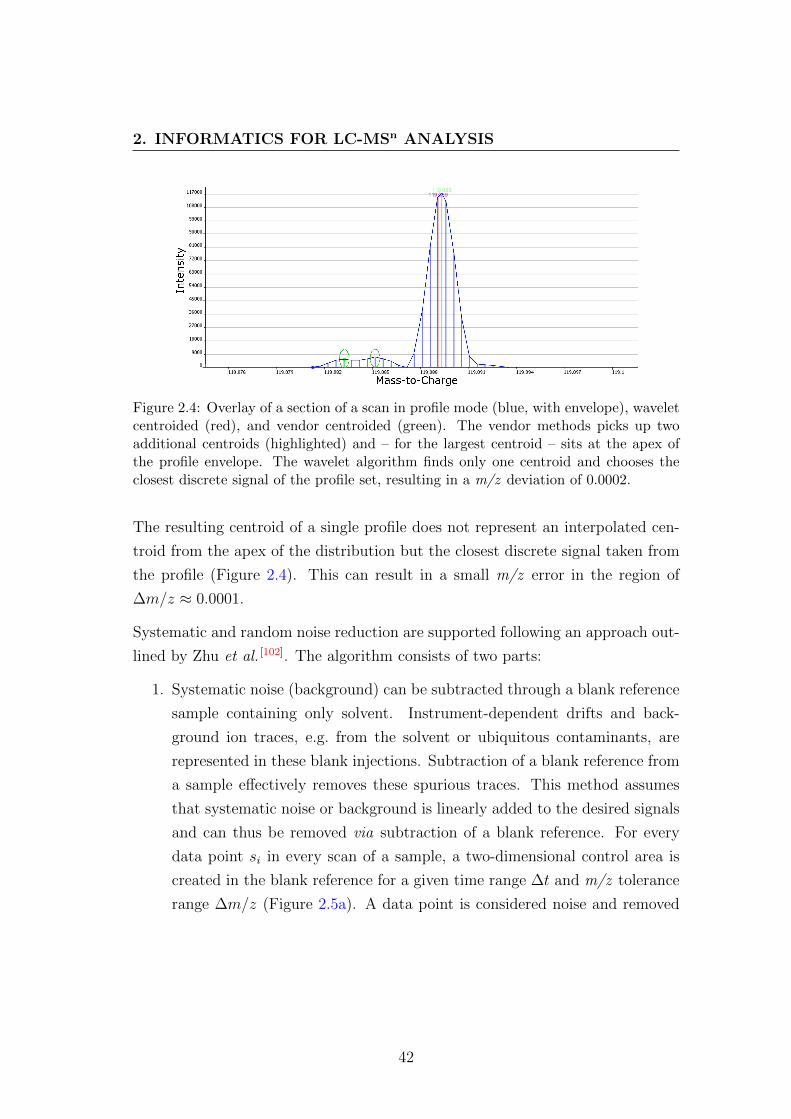
2. INFORMATICS FOR LC-MSn ANALYSIS
Figure 2.4: Overlay of a section of a scan in profile mode (blue, with envelope), waveletcentroided (red), and vendor centroided (green). The vendor methods picks up twoadditional centroids (highlighted) and – for the largest centroid – sits at the apex ofthe profile envelope. The wavelet algorithm finds only one centroid and chooses theclosest discrete signal of the profile set, resulting in a m/z deviation of 0.0002.
The resulting centroid of a single profile does not represent an interpolated cen-
troid from the apex of the distribution but the closest discrete signal taken from
the profile (Figure 2.4). This can result in a small m/z error in the region of
∆m/z ≈ 0.0001.
Systematic and random noise reduction are supported following an approach out-
lined by Zhu et al. [102]. The algorithm consists of two parts:
1. Systematic noise (background) can be subtracted through a blank reference
sample containing only solvent. Instrument-dependent drifts and back-
ground ion traces, e.g. from the solvent or ubiquitous contaminants, are
represented in these blank injections. Subtraction of a blank reference from
a sample effectively removes these spurious traces. This method assumes
that systematic noise or background is linearly added to the desired signals
and can thus be removed via subtraction of a blank reference. For every
data point si in every scan of a sample, a two-dimensional control area is
created in the blank reference for a given time range ∆t and m/z tolerance
range ∆m/z (Figure 2.5a). A data point is considered noise and removed
42

2. INFORMATICS FOR LC-MSn ANALYSIS
if a similar data point sj is present in the control area of the reference:
(m/z)si −∆m/z ≤ (m/z)sj < (m/z)si + ∆m/z (2.5)
tsi −∆t ≤ tsj < tsi + ∆t (2.6)
2. Data points resulting from random noise are removed by inspecting adjacent
scans in the same sample for similar data points (Figure 2.5b). A data point
si is considered noise and removed if it does not have a set of adjacent
neighbours S = sj, sj+1, ..., sj+n within a given m/z tolerance ∆m/z and
the total length of the chain of adjacent neighbours, i.e. the length of the
putative ion trace, falls below a scan number threshold n. In addition,
the data point or at least one of its adjacent neighbours has to exceed a
minimum intensity threshold Imin:
(m/z)si −∆m/z ≤ (m/z)sj < (m/z)si + ∆m/z (2.7)
length(S) ≥ n (2.8)
Imax(S) ≥ Imin (2.9)
Data filters operating in all three domains – time, m/z, and intensity – allow
raw data trimming. The chromatographic element of a LC-MS system can be
significantly inconsistent at the beginning and end of each run due to column
properties and the mobile phase mixture typically used at those phases. Regions
above or below a certain m/z value may not be of interest experimentally or
signals below a certain minimum intensity that have not been filtered out by
the instrument may be considered noise a priori. Data filters crop the data
based on threshold values or ranges and remove unwanted or unreliable data
segments.
Feature extraction refers to the detection and isolation of distinct ion traces. Fea-
tures are build using a simple adaptive incremental approach. Scans are visited
in chronological sequence. Every data point in a scan is either assigned to a pre-
viously created ion trace – originating at an earlier scan – or becomes the source
of a new ion trace. Only one data point per scan be assigned to an ion trace.
43

2. INFORMATICS FOR LC-MSn ANALYSIS
(a) Systematic noise removal (b) Random noise removal
(c) Total ion chromatograms before and after noise removal
Figure 2.5: Illustration of noise removal pre-processing methods. (a) Time versus m/zplot of signals pre (blue) and post (red, covering blue) systematic noise removal. Blueand green bands indicate the m/z tolerance window of the blue and green trace. Anion trace of the background reference (green) falls within the window of the upper tracearound 119.085. Consequently, the sample ion trace is removed. (b) Time versus m/zplot of signals pre (blue) and post (red, covering blue) random noise removal. Traceslower than eight successive scans are removed (circled). (c) Total ion chromatograms ofthe pre- (blue), post-processed (red) sample and background reference (green). Noisereduction dramatically reduces baseline distortions while leaving large features intact.
Assignment is conditional on the m/z value of the data point being closest to the
weighted average of all m/z values captured by the ion trace from previous scans
and falling within the given m/z tolerance calculated around the trace’s weighted
average (Figure 2.6). The weighted average is updated on every assignment based
44

2. INFORMATICS FOR LC-MSn ANALYSIS
Figure 2.6: Illustration of the feature extraction process. Data points of the ion tracem/z = 119.0984 are shown with regard to their individual m/z values (red) and inten-sity (blue). The red points demonstrate the m/z measurement error. The course of thecharacteristic m/z value determined by a weighted average is shown in green. After thetrace’s maximum, the value is set to 119.0984. Subsequent low-intensity values onlyintroduce marginal deviations.
on the data point’s intensity, placing higher emphasise on high-intensity, i.e. more
accurate, m/z values. Finally, an ion trace qualifies as feature if it exceeds a given
minimum length (number of adjacent data points) and the distribution’s apex is
above a minimum intensity threshold.
To eliminate baseline drifts in the absence of a blank reference, a morphological
Top Hat filter has been implemented acting on individual features. The specific
implementation is described by Herk et al. [232]. Top Hat by opening is applied,
i.e. erosion followed by dilation, with a structuring element B on a feature f
(Figure 2.7). Erosion shaves off the peaks and reduces their width. Following,
dilation widens the flattened peaks. It reconstructs the shape without the shaved
off peaks. By applying dilation after erosion, i.e. opening, the baseline under
the peaks is first estimated and can subsequently be subtracted from the original
feature. The structuring element is characterised by a window width in the time
domain where the baseline drift occurs. The element itself can be understood as a
simple window that defines the granularity of the method. A wider window width
is more coarse. Peaks within the window width are flattened and the resulting
baseline estimate is more conservative.
45

2. INFORMATICS FOR LC-MSn ANALYSIS
0
10000
20000
30000
40000
50000
60000
99 109 119 129 139 149 159 169 179 189 199 209 219 229 239 249 259 269 279 289 299Time [s]
Inte
nsity
Class
1.Input
2.Erosion
3.Dilation
4.Output
Figure 2.7: Illustration of the TopHat algorithm. The input chromatogram (1.Input)is eroded with a structuring element of length six resulting in the ‘peak-shaved’ greenline (2.Erosion). Dilation takes the eroded data and reconstructs the original shapeswithout the peaks (3.Dilation). Subtraction of the estimated baseline (3.Dilation) fromthe original input (1.Input) yields the baseline-corrected chromatogram (4.Output).
Dilation :(f ⊕B)(x) = max {f(x− x′)|x′ ∈ B} (2.10)
Erosion :(f B)(x) = min {f(x+ x′)|x′ ∈ B} (2.11)
Opening :f ◦B = (f B)⊕B (2.12)
TopHat :f ′ = f − (f ◦B) (2.13)
Note that ⊕ and indicate operations that should be understood as additions
and subtractions in a non-numeric context. Here, the application of the struc-
turing element widens and reduces the peak shapes. The symbol ‘◦’ indicates
function composition. The baseline subtracted from the original feature gives the
new baseline-corrected feature. The remaining features, after noise reduction,
feature extraction, and – if required – baseline correction, still contain many bio-
logically irrelevant features. To further narrow down the solution space to extract
only high-quality ion traces, two criteria have been implemented: The mass chro-
matographic quality from the Component Detection Algorithm (CODA) and the
Durbin Watson score based on a combination of CODA with a Durbin Watson
statistic [233].
46

2. INFORMATICS FOR LC-MSn ANALYSIS
The mass chromatographic quality ‘mcq’ describes the similarity between a raw
(length-scaled x(λ)i) and a smoothed (auto-scaled x(r, s)i) version of a feature.
xi denotes the intensity value at position i in the feature’s intensity vector. λ,
s, and r indicate that the value is length-scaled or standardised and smoothed.
Higher quality features that are less likely to be random variations have a score
closer to one. The smoothed and raw version of the signal region are almost
identical. Noisy features show greater discrepancy and give a score closer to zero.
The window width w defines the granularity of the method in the time domain
and n corresponds to the total number of data points of the feature.
mcq =1√n− w
n−w+1∑i=1
x(λ)ix(w, s)i {mcq ∈ < | 0 ≤ mcq ≤ 1} (2.14a)
x(λ)i =xi√∑ni=1 x
2i
(2.14b)
x(r)Ri =1
w
i+w−1∑k=i
xk (2.14c)
x(s)i =xi − µσ
(2.14d)
The mass chromatographic quality gives good results for baseline-free ion traces.
If solvent signals or baseline artefacts are present, the mcq score gets dispro-
portionally worse because the smoothed version of the feature appear to contain
more random signal. To reduce this problem, the Durbin Watson score ‘dw’ has
been implemented as alternative (Figure 2.8). It acts on elements x′ of the first
derivative of a feature and summarizes the relative change in the feature through
the normalized sum of squared intensities. For noisy features, the relative change
will give higher dw values. The window width w defines the granularity of the
method in the time domain.
dw =
∑wi=2
(x′i − x′i−1
)2∑wi=1 x
′2i
{dw ∈ < | 0 ≤ dw ≤ ∞} (2.15a)
x′i = xi+1 − xi (2.15b)
47

2. INFORMATICS FOR LC-MSn ANALYSIS
(a) Total ion chromatograms before and after Durbin Watson filtering
(b) (Total) ion traces pre-filter (c) (Total) ion traces post-filter
0
50000
100000
150000
200000
250000
300000
350000
400000
450000
Raw Systematic Noise Scan Filter Random Noise Feature Extraction Durbin WatsonPreprocessing Stage
Num
ber
of F
eatu
res
(d) Bar chart summarising pre-processing steps
Figure 2.8: Illustration of Durbin Watson filtering and bar chart summary of pre-processing steps. (a) Total ion chromatograms of the pre- (blue) and post-filtered (red)sample using a strict Durbin Watson filter (dw = 1.5). The green circles highlightareas of difference. (b) Close up of the unfiltered area around 224 s. (c) Close up of thefiltered area around 224 s. In (b) and (c) the total ion trace is shown in black, individualfeatures are shown coloured. Irregular features are removed by the Durbin Watsonfilter leaving only well behaved features. (d) Bar chart summarising the decrease of thenumber of features during pre-processing. The 260 fold reduction demonstrates thenecessity for pre-processing for efficient data handling.
48

2. INFORMATICS FOR LC-MSn ANALYSIS
The threshold values for the CODA and Durbin Watson filters depend on the
individual sample sets and need to be adjusted accordingly. For data exploration,
traversal of percentiles of the total score distribution is recommended. This way
the impact of lower quality signals, which may be relevant, can be evaluated on
the final model.
A Savitzky-Golay filter has been implemented for feature smoothing, increasing
the signal-to-noise ratio without distorting the ion trace. For high signal-to-noise
data, smoothing can recover ion traces that would be filtered out as noise by
other pre-processing methods. The data is assumed to be spaced equally (h = 1),
allowing the use of convolution coefficient (a) lookup tables. A smoothing window
of length n is convoluted over a feature and a polynomial Y of low degree k is
iteratively fitted through the data points that lie within the smoothing window.
The midpoint x of the smoothing window is replaced by the value derived from
the fitted function. The window indices are defined by z where the midpoint x
equals zero. Afterwards, intensities of smoothed features are restored to the same
magnitude of the raw feature to avoid distortion.
Y = a0 + a1z + a2z2 + a3z
3 + . . . akzk (2.16a)
z =x− xh
(2.16b)
To remove features that are believed to be genuine but not of experimental in-
terest, e.g. contaminants and interferrents, features can be filtered by their exact
ion mass, further trimming the data set.
2.3.2 Data Processing
Data processing addresses extracted features and refines those intra- and inter-
sample. Features need to be deconvoluted and peak-picked to isolate compounds
of similar or identical mass that eluted at different time points (Figure 2.9a).
A popular second derivative polynomial approach and a more robust modified
Bieman [113] approach have been implemented. For the first approach, a higher
order polynomial is fitted through coefficient-lookup. The second derivative of
49

2. INFORMATICS FOR LC-MSn ANALYSIS
the function determines the boundaries (zero-intercepts) and maximum intensities
(local minima/maxima) of individual peaks in the trace. The method is sensitive
to the quality of the initial polynomial fit and was found to be less effective
for diverse peak shapes. The modified Bieman algorithm for peak picking is
purely-shape based: it finds local minima (boundaries) and maxima (peak apices)
through iterative data point traversal from the ion trace’s global maximum. The
trace is split into individual peaks based on the slope of the declining trace (see
Stein et al. [113]).
For both deconvolution methods, intensity-based thresholds are in place to remove
low-level – noisy – signals. For the polynomial approach, the second derivative
needs to exceed a pre-defined threshold to qualify as separate peak. the Bieman
algorithm carries out a least squares background estimation from the lower half
of the total set of background-subtracted ion trace data points.
To remove retention time shifts across samples, Obiwarp – a tool for ordered
bijective interpolated warping – can be utilized [121]. The parameters required by
Obiwarp are extensively documented on its official web page and are mostly self-
explanatory, e.g. the parameters for gap initiation and extension penalties. Before
alignment of a collection of features of a sample to another collection of feature of
a reference, i.e. the adjustment of the feature landscapes, these collections need
to be binned in the time and m/z domain to create a regular grid that is shared
by all samples and the reference. Equidistant binning is used for both domains.
The smaller the bin size in either domain, the higher the resolution and more
fine-grained the resulting alignment. Too small bin sizes result in poor alignment
due to sparseness. Because MassCascade and Obiwarp store MS data differently,
binned grids are stored temporarily in Obiwarp-compatible ASCII ‘lmat’ format
for every sample and reference. Lmat files can subsequently be used as input for
Obiwarp, spawned in parallel in separate threads. Obiwarp returns a vector or
adjusted time values of equal length to the number of bins in the time domain
of the input grid. Nearest-point linear interpolation is used to translate these
adjusted time values into corrections for the unbinned features in the original
feature collection (Figure 2.9b).
50

2. INFORMATICS FOR LC-MSn ANALYSIS
(a) Bieman-based deconvolution (b) Obiwarp bin size response landscape
(c) Feature set: signals (d) Feature set: ion traces
Figure 2.9: Illustration of deconvolution, alignment, and feature set methods. (a) Ex-ample of Bieman-based deconvolution. The outer ion trace (blue, scaled up) representsthe chromatogram of a single ion. The green and red traces result from the decon-volution process. The original ion trace has been truncated at its local minima. (b)Response landscape of the mean difference of target-to-reference distances before (∆t)and after (∆t′) alignment with Obiwarp: ∆T = 1
n
∑ni=0 (|∆t′i| − |∆ti|), where n equals
the number of aligned features; the times ∆t and ∆t′ correspond to the differences in re-tention time rt: ∆t(
′) = tSr −tRr with S and R being the target and reference. Bin widthsin the time and m/z domain have been increased in steps of 0.5 from 0.1 to 3.0. Lower∆T values indicate better overall alignment. The graph shows that best alignment re-sults are achieved with larger bin sizes for the time domain, which should approximatethe time interval between scans. Obiwarp was run with default settings. (c) Spectrumand (d) ion traces of a feature set representing Cytidine ([M+H]+ = 244.092) groupedvia cosine similarity.
51

2. INFORMATICS FOR LC-MSn ANALYSIS
Atypical for LC-MS software, MassCascade does not compile fragmentation mass
spectra by default. One or more fragmentation spectra, i.e. MS2+, are typically
generated for selected precursor ions. For these ions, every MS1 scan results
in one or more MS2+ scans that are recorded . These can be collapsed into a
single representative fragmentation spectrum similar to ion extraction in MS1
(see paragraph 2.3.1). Representative fragmentation spectra of MS depth n are
subsequently assigned to the extracted feature (ion trace) of the precursor ion in
recursive fashion, e.g. for structure fragment assignment. Note that only selected
features with experimentally acquired MS2+ scans can have associated consensus
spectra. It should be noted that collapsed fragmentation spectra are consensus
spectra that only contain signals present in all fragmentation scans of a parent ion.
This process has been kept separate in line with the principle of modularity.
A collection of features is highly redundant by itself. Multiple signals can result
from a single molecular compound. Cosine similarity and a modified Bieman
approach have been implemented to group related features into feature sets (see
chapter 2.2).
The cosine similarity function creates a pairwise similarity matrix from all features
of a sample. To reduce memory load, only features within a pre-defined time
interval are considered simultaneously. Non-overlapping ion traces are excluded
by default. The spectral vectors, i.e. the features’ ion trace intensity vectors(~Ia, ~Ib
), are used to calculate their similarity (angle θ) using the dot product and
magnitude:
sim = cos(θ) =~Ia · ~Ib
‖ ~Ia ‖‖ ~Ib ‖sim ∈ {0 ≤ sim ≤ 1} (2.17a)
Correlated features show similarities greater than 0.95. Any features below the
defined similarity threshold are not clustered together in a single feature set
(Figure 2.9c and 2.9d). If multiple features exists that have overlapping but
gradually shifting ion traces, the algorithm will follow these shifts in the time
domain to group the features together. Higher similarity thresholds restrict that
behaviour automatically.
52

2. INFORMATICS FOR LC-MSn ANALYSIS
.0 .1 .2 .3 .4 .5 .6 .7 .8 .9
s=6s=8
6 8
s=9
9
17.6.6
Figure 2.10: Illustration of the modified Bieman algorithm to group related features.Overlapping features are binned in the time domain using a bin size of 10. Threefeatures are shown in gray, yellow, and brown. Individual features are binned bytheir sharpness value s, i.e. a value describing the steepest slope from their apex toa neighbouring data point (indicated by the red line). To estimate the uncertaintyrange, the number of bins is divided by the sum of values of populated neighbouringbins: 10
9+8 ≈ 0.6. If no bin within the uncertainty range contains a higher sharpnessvalue than the maximum value in the bins that gave rise to the uncertainty range,features captured in those bins are believed to be correlated (the yellow and brownpeaks). The figure is adapted from Stein et al. [113].
The modified Bieman approach uses a shape-based approach described by Stein et
al. [113], Figure 2.10. The granularity of the clustering can be adjusted by the num-
ber of bins. A single bin is defined by a given length (parameter A) divided by the
given number of bins (parameter B). For this method, the length should approx-
imate the distance of two adjacent scans for fine resolution. Higher length values
will yield larger feature sets with less similar features grouped together.
2.3.3 Data Post-Processing
The annotation and identification of features or feature sets forms the last part
of an LC-MSn analysis. The identification of metabolites is discussed in detail in
the next chapter. This section deals with the annotation and low-confidence iden-
tification only. MassCascade stores meta data extracted from raw files, such as a
53

2. INFORMATICS FOR LC-MSn ANALYSIS
sample’s ion mode, internally to simplify usage. Thus, the number of parameters
for annotation methods has been reduced to the greatest degree possible because
information about MSn levels or ion modes does not need explicit input.
Adducts, neutral losses, and any other relations that are based on differences of
m/z signals within a feature set can be annotated: pairwise signals for which a
relationship evaluates to ‘true’ are annotated with the corresponding feature iden-
tifiers and type of relationship (Figure 2.11a). For example, a m/z difference of
21.9819 represents a replacement of a hydrogen atom with a sodium atom in pos-
itive ion mode: [M+H]+ → [M+Na]+. Feature sets can be queried for any two-
column list of annotations and m/z differences. The m/z differences are matched
for every feature pair within a given ppm tolerance. Comprehensive adduct and
neutral loss lists have been published that can be used as template [110].
Isotopes are detected using a combinatorial approach with a quality check for
final assignment based on a heuristic model. The average isotope difference is set
to ∆mz = 1.0033 [234]. Isotopic signals can be detected up to a distance of three,
i.e. [M+3]. Abundances of single-step isotopic signals with distances greater than
three are considered to be of too low intensity to be relevant: with an isotopic
abundance of 13C = 1.10, C66 would result in a signal at [M+4] that equals
1% of the intensity of the main signal. Elements that have ‘irregular’ isotopic
patterns, e.g. 32S = 95.02%, 33S = 0.75%, 34S = 4.21%, are not fully detected. A
m/z tolerance can be defined in ppm to account for mass defects. The algorithm
sorts all features of a feature set in ascending m/z order before traversing the
list in recursive fashion, pairwise matching all features lower in the list to the
current index. If a m/z difference equals the theoretical isotope difference, the
relative intensity of the isotope signal, i.e. its intensity divided by the main signal
intensity, is matched to the theoretical relative intensity of an isotopic signal
within the corresponding m/z range in which the signal falls. A positive match
results in isotope annotation.
The heuristic model for the theoretical relative intensity of m/z ranges was de-
rived in the following way: small molecules were downloaded in bulk in SD-
File format from the metabolomics databases HMDB [235], Golm [236], and Mass-
Bank [237]. Molecular formulas were extracted and filtered for subsets contain-
54

2. INFORMATICS FOR LC-MSn ANALYSIS
(a) Isotope and identity annotations for Cytidine
(b) Diagram of feature identification methods and their mode of action
Figure 2.11: Illustration of annotation and identification methods. (a) Feature set(compound spectrum) of Cytidine (structure shown) with annotations for isotopes asperceived by MassCascade. Relations such as the Cytidine cluster (Cyt-2) or its sugar-removed fragment (Cyt-Sugar) were annotated through a list with m/z differences. (b)Diagram of feature or feature set identification methods including their mode of action.ChemSpider, Metlin, and MassBank are online databases. Reference library and m/zlist queries are local operations. Whereas a ‘Spectrum match: MS1+’ matches thefeature set at MS1 as well as relevant fragmentation spectra (MS2+), the ‘Parent ion &MS2+’ match by Metlin only matches a single feature in MS1 and subsequently proceedsto its fragmentation spectra. Matching features are annotated with a small molecule’sdatabase identifier, chemical name, line notation (SMILES or InChI if provided), andquery score.
55

2. INFORMATICS FOR LC-MSn ANALYSIS
0.00
0.05
0.10
0.15
0.20
0.25
0.30
0.35
0 500 1000 1500 2000 2500Molecular Mass
Rel
ativ
e A
bund
ance
Isotope_Ratio
1
2
3
Figure 2.12: Linear regression for molecular masses vs. isotope abundances. Data seriesfor isotope ratios 1 (red), 2 (green), and 3 (blue) are shown. The molecular masses andtheoretical isotope patterns were calculated from the molecule collections of HMDB,Golm, and MassBank.
ing only the elements CHNOPS + F + Cl. Bromide was excluded because
of its atypical isotopic abundance pattern, 79Br = 50.69%, 81Br = 49.31%,
which would significantly skew the relative intensity distribution for isotopic
distances. Sulfur, 32S = 94.93%, 33S = 0.76%, 34S = 4.29%, and Chlorine,35Cl = 75.78%, 37Cl = 24.22%, did not impact significantly on the intensity dis-
tribution. Their isotopic abundance patterns’ ‘irregularities’ were absorbed in the
overall measurement error. The representative, non-unique set contained 47,849
molecular formulas. The theoretical isotopic envelopes were calculated for the
whole set and a linear regression applied for the relative intensities of every iso-
topic ratio (Figure 2.12). The resulting linear formulas of form I = a ∗m/z + b
describe the deduced intensity I for any m/z with the coefficients a and b.
Putative feature or feature set identifications, i.e. metabolite annotations, are
facilitated by methods for direct ion identification, local library queries, and web-
based searches (Figure 2.11b). Direct ion identification refers to simple m/z
lookup in a reference list that can directly be fed into MassCascade. The reference
list has to contain exact molecular masses and molecule labels. The molecular
masses are automatically (de-)protonated based on the ion mode.
56

2. INFORMATICS FOR LC-MSn ANALYSIS
Local library queries depend on the creation of a ReferenceContainer instance,
containing ReferenceSpectrum instances. The reference spectra have a m/z -
intensity list for each set MS level and compound information such as the name,
line notation, molecular mass, and formula. Fragmentation spectra are traversed
if defined. Local queries are dramatically faster than web-based searches.
Web-based searches include the databases ChemSpider [186], MassBank [237], and
Metlin [238]. ChemSpider and Metlin queries require a security token issued by
the individual websites. For the databank ChemSpider a subset of databases
can be selected for simple m/z lookups from the total list of databases available.
The MassBank and Metlin integration offers feature set (MS1) and fragmentation
spectra matching (MS2+) in addition to simple m/z lookups, resulting in more
reliable feature annotation. Input parameters correspond to the web interfaces.
Results from local or web-based queries are assigned to the respective features
or features sets including the chemical name, line notation (SMILES or InChI),
query score, and database identifier.
2.4 MassCascade for KNIME
A plug-in for the workflow environment KNIME has been developed. The plug-
in MassCascade-KNIME wraps the functionality of the MassCascade core library
and exposes the functions as graphical nodes. A node can be considered an atomic
unit of interaction. Manipulator nodes take one to many inputs and produce one
to many outputs. Source nodes take no input from other nodes whereas sink
nodes do not pass any output further. Similar to a scripted pipeline, individual
functions, i.e. nodes, can be inserted or deleted at any point in the workflow.
2.4.1 Structure
The plug-in serves as interface between the open-source platform KNIME and the
MassCascade library. It manages node-user and node-node interactions and de-
legates jobs to the task classes of its back-end. These jobs are grouped into three
57

2. INFORMATICS FOR LC-MSn ANALYSIS
(a) Plug-in architecture (b) KNIME node model
Figure 2.13: Overview of the MassCascade-KNIME architecture and KNIME’s nodemodel. (a) The plug-in forms part of the KNIME Desktop and serves as interface be-tween the three frameworks of the MassCascade library and the KNIME workbench.(b) The adapted KNIME node model distinguishes between source, sink, and manip-ulator nodes. These node types have distinct input and output ports and facilitateintuitive usage of the plug-in. The ‘traffic light’ color scheme indicates the state of anode: Executed nodes are green, configured nodes are yellow, and unconfigured nodesare red.
categories based on their purpose: jobs that address the core framework (data
processing), the visualisation framework (plots and charts), or the identifica-
tion framework (signal or spectrum identification, rationalisation of results) (Fig-
ure 2.13a). Each category is handled differently in the plug-in (section 2.4.3).
In contrast to the internal design, nodes are grouped by the kind of interaction
they provide: Source nodes read data from files or convert external tabular data
to a format that can be processed by the plug-in, manipulator nodes change the
data, sink nodes write data to files or convert internal tabular data to generic
data types, and visualisation nodes provide views of data in tabular or graphical
form (Figure 2.13b).
Underneath the nodes, data processing jobs are executed concurrently using
Java’s R© concurrency framework [229]. Each thread deals with a single sample,
i.e. reads the data container, applies a function, and writes the data out into
a new container. The number of threads available depends on the global confi-
guration of KNIME. Raw data is serialized to disk by the MassCascade library
in a temporary directory specified by the user whereas access pointers to the
58

2. INFORMATICS FOR LC-MSn ANALYSIS
raw data are stored through KNIME’s persistence framework. Employing this
split serialisation scheme guarantees efficient data handling: The KNIME plug-in
only deals with small XML-based files that contain pointers to large data chunks.
These small files can be modified and swapped back and forth between nodes at
low cost, e.g. memory. For operations on the LC-MSn data, the files are con-
verted to their respective container types and passed on to the main task class.
The main task class reads the data on demand and returns a new container, as
described in section 2.2. The returned container is again serialised to XML for
persistence.
2.4.2 Node Types
Nodes of different types can be concatenated to build a workflow as depicted
in Figure 2.14. Every MassCascade-KNIME workflow must start with a source
node and typically ends with a sink node to output results. Manipulator nodes
in between a source and sink node are for data processing. Visualisation nodes
can be employed at any step in the workflow to inspect the data at that node.
In contrast to all other node types, visualisation node types do not require any
input parameters.
Figure 2.14: Typical MassCascade-KNIME workflow demonstrating how different nodetypes can be used in combination. LC-MSn files are read in via the File Reader nodebefore the extraction of meta information. Following, random noise is eliminated andfeatures are extracted. The features are converted to a generic tabular KNIME formatthat can be used with generic KNIME nodes. The Spectrum Viewer allows interactiveinspection of the noise-reduced samples.
59
2. INFORMATICS FOR LC-MSn ANALYSIS
2.4.3 Node Interactions
Two types of node interactions are distinguished: Node-node and node-user in-
teractions. Both types of interactions are defined by the plug-in. To render
the node coding process more efficient, abstract custom models have been built
on top of the four key parts of a default KNIME node model (see section 1.2.4).
These abstract classes are extended by all MassCascade-KNIME nodes, enforcing
standardised behaviour across all interactions levels and reducing time spend de-
veloping nodes (Figure 2.15). Because of the common base classes, any new node
implementation requires only the implementation of a model and – if required –
view, in addition to the definition of node parameters.
Node-Node Interactions
Node-node interactions are based on KNIME’s tabular data model (see sec-
tion 1.2.4). Three distinct data cell types have been developed to represent MS,
profile, and spectrum data containers of the core library (see section 2.2). In-
stances of these cell types are serialized to disk for persistence by the KNIME
environment. Node-node interactions are only possible when a required input cell
type of one node matches an output cell type of a preceding node. This compa-
tibility of cell types is enforced by an automated mechanism in the DefaultModel
class. Input or output of multiple data tables must be specifically provided in
the model implementation but follows the same principle. MassCascade cells
types depict their content in KNIME tables: MS data cells sketch a total ion
chromatogram, profile data cells depict a histogram of time bins (ascending) to
number of binned profiles, and spectrum data cells show a plot of time versus
m/z values, where every point represents a found profile.
Node-User Interactions
Node-user interactions are provided through node dialogues, depictions, input-
output tables, and data views. MassCascade-KNIME provides interactive param-
eter dialogues with parameter validation, default values, and auto-configuration
60

2. INFORMATICS FOR LC-MSn ANALYSIS
Fig
ure
2.1
5:S
chem
atic
of
the
nod
earc
hit
ectu
rean
din
tera
ctio
ns.
Th
ege
ner
icK
NIM
Ecl
asse
sh
ave
bee
nex
tend
edto
crea
teab
stra
ctd
efau
ltcl
ass
esto
sim
pli
fyth
ed
evel
op
men
tpro
cess
.T
he
Def
au
ltS
etti
ngs
clas
sli
nks
the
con
figu
rati
ond
ialo
gue
and
node
mod
el,
savin
gan
dlo
ad
ing
all
nod
ep
aram
eter
s.T
he
Def
au
ltD
ialo
gcl
ass
isa
tem
pla
teth
atb
uil
ds
con
figu
rati
ond
ialo
gues
on-t
he-
fly
base
don
pre
-defi
ned
bu
ild
ing
blo
cks.
Itlo
ads/
saves
nod
ep
aram
eter
sto
/fro
mth
ed
efau
ltse
ttin
gscl
ass.
Th
eD
efau
ltM
odel
class
pro
vid
esp
aram
eter
vali
dat
ion
and
han
dle
sn
od
eex
ecu
tion
.It
take
sa
set
ofin
pu
tta
ble
san
dp
rod
uce
sa
set
ofou
tpu
tta
ble
s.T
he
Def
au
ltV
iew
class
vis
ual
ises
dat
aex
pos
edth
rou
ghth
eD
efau
ltV
iew
Mod
elcl
ass
inth
efo
rmof
gra
ph
ical
chart
s.
61

2. INFORMATICS FOR LC-MSn ANALYSIS
(a) Noise Reduction node dialogue (b) Profile Converter node dialogue
Figure 2.16: Configuration dialogues of the (a) Noise Reduction and (b) Profile Con-verter nodes. The dialogues take a set of input parameters in the ‘Parameters’ sectionand define the required input cell type in the ‘Source’ section of the tab.
(Figure 2.16). Erroneous parameters are not accepted and render the node dis-
abled. Node dialogues are loaded with default parameters. Auto-configuration
checks if the input table(s) contain the data types required. The outcome of
the node configuration is reflected in the traffic light representation of the nodes’
execution status.
Data views visualise data cells of a particular type. Execution of the visualisation
nodes does not change data in the respective data cells. All visualisation nodes
follow the same layout: input data cells are listed on the right of the visualisation
window, optionally with an added section for further listings for loading data.
The main part of the window is taken up by an interactive two dimensional
plot. Depending on the individual node, plots offer different data representations,
accessible via the file menu (Figure 2.17).
62

2. INFORMATICS FOR LC-MSn ANALYSIS
Figure 2.17: Demonstration of the Spectrum Viewer node. The central area of thewindow shows two spectra selected via the spectrum list in the bottom right. The datacells for the spectrum list are shown in the top right.
2.5 Evaluation
2.5.1 Spectral Fingerprinting of Tomato Samples
Metabolomic fingerprinting is one of the key applications of LC-MSn. Metabolomic
fingerprinting is based on a sample by feature matrix, where features have reliably
been found across samples. These features are believed to be characteristic for the
samples and can thus be used for multivariate clustering and subsequent genera-
tion of predictive models. Fingerprinting relies on the extraction of real features,
i.e. m/z -intensity value pairs that represent ions stemming from metabolites, and
on correct alignment of features across samples to generate the feature matrix.
The quality of the resulting matrix depends heavily on the feature extraction
and alignment process, as well as on the overall data pre-processing. Insufficient
or incorrect data pre-processing could introduce noise to the matrix in the form
of irrelevant features, e.g. m/z -intensity value pairs that stem from background
ions or impurities, or incorrect features, e.g. value pairs that do not exist or are
not present in all samples indicated. This matrix would show a higher level of
unexplainable variance and could lead to wrong clustering.
63

2. INFORMATICS FOR LC-MSn ANALYSIS
MassCascade was tested for correct fingerprinting using a data set of aliquots
of a pooled standard tomato control with known clustering. The test allows for
exploration of various aspects of the tool, including feature extraction, deconvo-
lution, and alignment, and provides a statistical measures for the quality of the
generated feature matrix.
2.5.2 Materials and Methods
The data set was provided by the Syngenta AG. The data was acquired using
aliquots of a polar extract from wild-type tomato (Solanum lycopersicum), which
was used as pooled in-house control. The 113 samples were used as controls in a
long-term study at the Syngenta AG (section 2.1). Approximately 30 mg of dried
tomato tissue was extracted with ethanol:water 20:80 (v/v) and diluted 10:1 (v/v)
with water for injection. A mixture of citric acid-d4 [CID 16213286], L-alanine-d4
[CID 12205373], glutamic acid-d5 [CID 56845948], and L-phenyl-alanine-d5 [CID
13000995] was added for internal calibration. The samples were measured on a
Thermo Velos Orbitrap coupled to a Waters Acquity UPLC with a HSS T3 150 x 2
mm, 1.7 µm, Acquity UPLC column. The solvents used for the assay consisted of
0.2% formic acid (solvent A) and 98/2/0.2 acetonitrile/water/formic acid (solvent
B). The gradient started at 100% A (hold 2.5 minutes) at 0.25 mL/min followed
by a ramp to 10% B after 7.5 minutes increasing the flow rate of 0.4 mL/min; then
to 100% B after 10 minutes, hold 2 minutes, before equilibrating back to starting
conditions after 18 minutes. The samples were detected in positive ESI mode
at a resolving power of 30,000 FWHM with a scan range from 85-900 Da. MS2
spectra were obtained in a data dependent manner: The two most intense mass
spectral peaks detected in each scan were fragmented to give MS2 spectra. Full
scan data was acquired in profile mode, MS2 spectra were acquired in centroid
mode.
The data files were converted from Thermo Scientific’s RAW format to mzML
using ProteoWizard v2.2 [230] with vendor-based peak picking enabled for MS1.
The data were processed using the MassCascade plug-in for KNIME, following
the steps outlined in Figure 2.18. Feature extraction was carried out with 10
64

2. INFORMATICS FOR LC-MSn ANALYSIS
September October January March
Date Count Date Count Date Count Date Count
2010-09-17 4 2010-10-04 1 2011-01-18 6 2011-03-22 4
2010-09-18 9 2010-10-05 8 2011-01-19 7
2010-09-20 7 2010-10-06 15
2010-09-21 14 2010-10-07 10
2010-09-22 9 2010-10-08 15
2010-10-09 4
Table 2.1: Overview of the number of wild-type tomato samples measured by date.The samples were measured over a total of four months.
ppm mass accuracy. A minimum width of six scans and a minimum intensity of
100,000 units was used for thresholding of features. In addition, a Durbin-Watson
statistic was used to filter out features that were assigned a score above the third
quartile of the normal score distribution taken from all features, here Qdw3 = 2.38.
Deconvolution was applied with a signal to noise ratio of two using a modified
Bieman algorithm. Obiwarp was used for cross-sample alignment with default
parameters and aligned features subsequently filtered and selected for presence
of isotopic peaks. Features associated with common interferents were removed.
Figure 2.18: Flow diagram depicting LC-MS data processing steps for metabolomicfingerprinting. After random noise reduction, features are extracted and filtered usinga statistic describing expected chromatographic behaviour. The filtered features aresmoothed in the time domain and deconvoluted to resolve overlapping isobaric features.Found features are matched across all samples of a group, filtered for presence of isotopicpeaks for selectivity, and written out in feature matrix. Subsequently, intensity gaps inthe matrix are filled before multivariate analysis.
65

2. INFORMATICS FOR LC-MSn ANALYSIS
The aligned features were written out in a feature matrix and gap filling was
applied: gaps were filled with intensity values from the baseline of the individual
samples at the features’ retention times and m/z values. If no baseline value
could be found, gaps were assigned a default intensity of 10,000 units. A total of
11 result matrices were compiled with allowed missingness ranging from 0-100%
in 10% increments. The matrices were subjected to multivariate analysis in the
statistical computing environment R.
2.5.3 Results
Initial inspection of the total ion chromatograms of all samples revealed two
failed injections for samples 2010-10-09 12 and 2010-10-09 13. Both samples
contain only baseline noise with no apparent features and were removed from
analysis. Cross-sample comparison of mean-centered total ion currents showed
significantly higher intensities for samples 2011-0322 01, 2011-03-22 02, 2011-03-
22 03, and 2011-03-22 04, likely due to wrong sample preparation or over-injection
(Figure 2.19). All four March samples were flagged as outliers and kept.
Sample 2010-09-21 61 was chosen as reference for the feature-based alignment
with Obiwarp based on its representative total ion current and shape of its total
ion chromatogram, minimising overall time shift. The result of the non-linear
alignment is depicted in Figure 2.20a. The stability of the column measured by
sample to reference time deviation appears to dependent on the acquisition date.
Time shifts of features grow bigger with an increase in the time gap between
sample and reference. Samples acquired on the same date show the least varia-
tion in time shifts, followed by variation in between groups acquired in the same
month. This was to be expected. Even though the same instrument was used for
all measurements, it was not used exclusively for the study. Other experiments
were run on the Orbitrap in between the months. Thus, column modifications
such as degradation or insufficient equilibration become more apparent over time.
All samples show uncorrelated shifts before about 80 s and after 750 s, coinciding
with the dead time of the system and end point of the solvent gradient respec-
tively.
66

2. INFORMATICS FOR LC-MSn ANALYSIS
(a) Total ion currents
(b) Total ion chromatograms
Figure 2.19: Summary of the sample intensity domain. (a) The mean-centered total ioncurrent for each sample is shown in red. The blue line indicates zero intensity. Samples16, 51, 53, and 62 represent the four March samples and show significant deviation fromthe trend. Samples 43 and 108 refer to 2010-10-09 12 and 2010-10-09 13 and containbaseline noise only, explaining the strong negative deviation. (b) Overlay of all totalion chromatograms coloured by date. All chromatograms have similar shape. The fourMarch samples are clearly distinct with dramatically higher intensities. The samplesshow slight time deviation and increasing baseline drift from 570 s.
67

2. INFORMATICS FOR LC-MSn ANALYSIS
(a) Time - shift regression
(b) m/z - shift regression
Figure 2.20: Summary of the feature alignment. The data points and regression curvesare coloured by acquisition date. (a) Plot of the elution time versus time shift, i.e. thetime difference before and after alignment. A polynomial regression fit was used. Theregression curves are coloured by acquisition date. Samples measured on the same datecluster together. Shifts before about 80 s and after 750 s appear to be uncorrelated. (b)Plot of the m/z values versus time shift with a polynomial regression fit. The lineartrends show that the time shift is almost constant for all m/z values, indicating nocorrelation between mass-to-charge ratio and time shift.
68

2. INFORMATICS FOR LC-MSn ANALYSIS
2010−09−17
−40
−30
−20
−10
0
10
20
30
40
0 100 200 300 400 500 600 700 800 900
2010−09−18
−40
−30
−20
−10
0
10
20
30
40
0 100 200 300 400 500 600 700 800 900
2010−09−20
−40
−30
−20
−10
0
10
20
30
40
0 100 200 300 400 500 600 700 800 900
2010−09−21
−40
−30
−20
−10
0
10
20
30
40
0 100 200 300 400 500 600 700 800 900
2010−09−22
−40
−30
−20
−10
0
10
20
30
40
0 100 200 300 400 500 600 700 800 900
2010−10−04
−40
−30
−20
−10
0
10
20
30
40
0 100 200 300 400 500 600 700 800 900
2010−10−05
−40
−30
−20
−10
0
10
20
30
40
0 100 200 300 400 500 600 700 800 900
2010−10−06
−40
−30
−20
−10
0
10
20
30
40
0 100 200 300 400 500 600 700 800 900
2010−10−07
−40
−30
−20
−10
0
10
20
30
40
0 100 200 300 400 500 600 700 800 900
2010−10−08
−40
−30
−20
−10
0
10
20
30
40
0 100 200 300 400 500 600 700 800 900
2010−10−09
−40
−30
−20
−10
0
10
20
30
40
0 100 200 300 400 500 600 700 800 900
2011−01−18
−40
−30
−20
−10
0
10
20
30
40
0 100 200 300 400 500 600 700 800 900
2011−01−19
−40
−30
−20
−10
0
10
20
30
40
0 100 200 300 400 500 600 700 800 900
2011−03−22
−40
−30
−20
−10
0
10
20
30
40
0 100 200 300 400 500 600 700 800 900
Time [s]
Tim
e S
hift
[s]
Figure 2.21: Overview of the feature alignment groups. The matrix shows the individualregression plots for all sample groups. The elution time versus time shift is plotted witha polynomial regression fit.
The individual groups are shown in Figure 2.21. The mass-to-charge values seem
to be uncorrelated to time shifts and have no impact on the alignment (Fig-
ure 2.20b).
Removal of common interferents (see appendix section 5) in LC-ESI-MS reduced
the number of features by an average of 212 per sample. The matched features
show no significant differences in their distributions compared to the remaining
features (Figure 2.22a). Table 2.2 lists the top five most frequently found contam-
inants. N-methyl-2-pyrrolidone, oleamide, and polyethylene glycol are believed
to come from laboratory equipment used in sample preparation. The acetoni-
trile/acetic acid species stems from the mobile phase. Its putative sodium adduct
shows a higher mass deviation of 19.0 ppm. The mass chromatograms of both
species were compared to verify that they are related. They co-elute at various
69

2. INFORMATICS FOR LC-MSn ANALYSIS
time points during the runs with the acetonitrile/acetic acid species present in
all samples and the sodium adduct absent in up to 11 samples, in consistence
with the assumption that the adduct is detected less often than the main species.
Comparison of the shapes of the feature mass chromatograms at 333 s support
this finding of a main species to sodium adduct relationship (Figure 2.22b).
(a) Intensity boxplot
(b) Mass chromatograms of two interferents
Figure 2.22: Summary of the interferents analysis. (a) Boxplot of the intensity distribu-tion of features versus filtered out interferents. No outliers are shown. The distributionsare not significantly different. (b) Mass chromatograms of the acetonitrile/acetic acidspecies (blue) and its sodium adduct (red) at 333 s. Both species coelute and have simi-lar elution profiles. The high-intensity chromatograms are artefacts from the erroneousMarch samples.
70

2. INFORMATICS FOR LC-MSn ANALYSIS
Name Sum Formula Mass Deviation Ion Type
N-Methyl 2-pyrrolidone C5H10NO 0.8 ppm [M+H]+
Acetonitrile/Acetic acid (CH3CN)n(CH3COOH)m 0.5 ppm [A1B1+H]+
Acetonitrile/Acetic acid (CH3CN)n(CH3COOH)m 19.0 ppm [A1B1+Na]+
Oleamide C18H35NO 0.5 ppm [M+H]+
Polyethylene glycol [C2H4O]nH2O 0.6 ppm [A2B+H]+
Table 2.2: Overview of the five most common interferents. The table shows the com-pound name, sum formula, mass deviation in ppm between the exact theoretical andfound ion mass, and ion type found.
After alignment, features before 80 s and after 750 s were filtered out before iso-
tope detection and compilation of the feature matrix for multivariate analysis.
The data set was split into two. In the first data set (‘filtered’), all features
without isotope information were filtered out. The second data set contains all
features (‘unfiltered’). Isotopic envelopes serve as additional orthogonal informa-
tion to improve confidence in extracted features. A data set filtered for isotopes
can serve as sanity check for data analysis because features with isotopic en-
velopes are less likely to be irrelevant artefacts. Both data sets were used to
investigate how incremental missingness affects the result matrix. Missingness is
defined as percentage of absence for a feature across samples, i.e. the number of
gaps. Higher missingness allows more features to be included in the matrix but
may potentially distort downstream analysis. Zero missingness is ideal but im-
practical because of imperfections of the instrument and in data processing. The
filtered and unfiltered data sets behave identical with regard to missingness (Fig-
ure 2.23a). The number of aligned features increases with allowed missingness,
with a steep increase from 90% to 100%. Maximum missingness includes features
that are only present in one sample, which should be considered unreliable. Step-
ping up to 100% missingness includes the bulk of features from unfiltered noise,
hence the increase in aligned features. At 0% missingness, a total of 23 and 165
features are observed in the filtered and unfiltered data respectively. The number
of gaps doubles with every 10% increase in missingness.
71

2. INFORMATICS FOR LC-MSn ANALYSIS
0
10
20
30
40
50
60
70
80
90
100
0 10 20 30 40 50 60 70 80 90 100Missingness [%]
Fea
ture
s [%
]
Gaps [%]
0
25
50
75
100
Group
Filtered
Unfiltered
(a) Missingness bubble plot
0
50
100
150
200
250
300
350
400
450
500
550
600
650
700
750
800
850
900
950
1000
0 5 10 15 20 25 30 35 40 45 50 55 60 65 70 75 80 85 90 95 100 105 110 115Sample
Abu
ndan
ce [u
nits
]
Compound
Citric acid−d4
Glutamic acid−d5
L−Phenyl−alanine−d5
(b) Compound intensity plot
Figure 2.23: Overview of the sample by feature missingness analysis. (a) Bubble plot ofthe missingness versus number of features, expressed in percent relative to the numberof features at 100% missingness. The plot shows a steep increase at 90% to 100%, wherefeatures only present in one sample are accepted in the matrix. At 0% missingness,165 features can be observed in the unfiltered data. The area of the data points cor-responds to the number of gaps (percent relative to the total number of gaps at 100%missingness). The number of gaps double with every 10% increment in missingness. (b)Line plot of the sample index versus intensity of Citric acid-d4, Glutamic acid-d5, andL-phenyl-alanine-d5. Intensity spikes can be observed for all March samples at index16, 51, 53, and 52. No spike is present for L-phenyl-alanine-d5 at position 16 due tomisalignment.
72

2. INFORMATICS FOR LC-MSn ANALYSIS
Name CID Sum Formula Exact Mass [M+H]+
Citric acid-d4 16213286 C6H4D4O7 196.05211 197.05939
L-alanine-d4 12205373 C3H3D4NO2 93.07279 94.08006
Glutamic acid-d5 56845948 C5H4D5NO4 152.08454 153.09182
L-phenyl-alanine-d5 13000995 C9H6D5NO2 170.11036 171.11764
Table 2.3: Overview of the deuterated internal standards. The table shows the com-pound name, PubChem compound identifier (CID), molecular formula, exact mass forthe deuterated compound, and exact mass for the main ion in positive ion mode.
Gaps are highly undesirable and typically need to be filled for most multivariate
methods. This introduces an element of uncertainty about why the signal is
absent in the sample and about the method to be used for gap filling. Gaps were
filled by reverse lookup of background signals in the raw data or, in the absence
of a background signal in the vicinity of the feature’s m/z value and retention
time, a default value of 100,000 was set.
Given the identical behaviour of the filtered and unfiltered data sets with regard
to missingness, the features in the unfiltered data set were assumed to be re-
presentative for the samples. The filtered data set was discarded. A maximum
missingness of 10% enabled the detection of the internal standards (Figure 2.23b),
resulting in a matrix with 680 features, and was chosen as optimum value. The
standards listed in Table 2.3 were identified within a mass accuracy of 10 ppm.
Spikes in abundance can be noted for the internal standards of all four March
samples, similar to what is shown in Figure 2.19a, with the exception of sample
2011-03-22 04 at position 16, where no feature was found for L-phenyl-alanine-d5
and gap filling was applied. The missing feature was incorrectly aligned and was
skipped by the semi-automated analysis process. L-alanine-d4 was removed from
the analysis because of its retention time at 85 s, which is borderline to the time
filter at 80 s. The compound was only detected in 60% of all samples in this
inconsistent region.
73

2. INFORMATICS FOR LC-MSn ANALYSIS
The resulting feature matrix was used for principal component analysis (PCA).
The matrix containing 111 samples and 680 features was autoscaled before it was
subjected to PCA. The result is shown in Figure 2.24a, where the first two com-
ponents explain 60% of the variance (Figure 2.24b). The four March samples are
distinct outliers and distort the analysis because of their high feature intensities.
The samples were removed before re-analysis. The corrected matrix is shown in
Figure 2.25a. The explained variance is still 60% but with greater contribution
from the second principal component (Figure 2.25b). The PCA reveals distinct
clustering of samples by date. Ideally, all samples should be indistinguishable
because of the lack of biological variation. The differences could result from sam-
ple preparation, data acquisition, or data processing. Given that the whole data
set was batch processed and the variation is not random, invalid data processing
can be ruled out. The strong clustering by sample date indicates instrument-
introduced variation under the assumption that the minor errors during sample
preparation were random. The observed inter-aliquot variation disappears when
biologically different samples are introduced (see section 3.5, Figure 3.4).
A drift can be noted for five samples acquired on 2010-09-21. Isolation of that
sample group and analysis of the intensity distributions, reveals that samples
acquired earlier on the day (index 2, 3, 9, 15, and 20) have shifted distributions
towards higher intensities (Figure 2.26). Even though the shift is not significant,
it is picked up in this analysis due to the absence of big variation, e.g., biological
variation. This shift is responsible for the drift observed in the PCA.
In this case study, MassCascade was used to process LC-MSn data of 113 quality
control samples from wild-type Solanum lycopersicum. Because of the lack of bio-
logical variation, variation introduced by sample preparation and instrumentation
could be picked up. The clustering seen in PCA are non-random and could be
explained, ruling out significant errors through the actual data processing. This
demonstrates that MassCascade can be used for fingerprinting experiments and
data exploration.
74

2. INFORMATICS FOR LC-MSn ANALYSIS
Ellipse: Hotelling’s T2 (95%)−15
−10
−5
0
5
10
15
20
−40 −30 −20 −10 0 10 20 30 40 50 60 70 80 90 100 110PC1
PC
2
Groups
2010−09−17
2010−09−18
2010−09−20
2010−09−21
2010−09−22
2010−10−04
2010−10−05
2010−10−06
2010−10−07
2010−10−08
2010−10−09
2011−01−18
2011−01−19
2011−03−22
(a) Principal component analysis
0
5
10
15
20
25
30
35
40
45
50
55
60
1 2 3 4 5 6 7 8 9 10 11 12 13 14 15Principal Component
Exp
lain
ed V
aria
nce
[%]
(b) Variance explained by PCs
Figure 2.24: (a) Principal components analysis of the aligned features of all samples.The samples are coloured by acquisition date. A confidence region is shown as ellipseusing Hotelling’s T2 statistic. The March samples are strong outliers, obfuscating theplot. (b) Bar chart of the explained variance by principal components in percent. Thefirst two principal components explain 60% of the overall variation.
75

2. INFORMATICS FOR LC-MSn ANALYSIS
Ellipse: Hotelling’s T2 (95%)
−35
−30
−25
−20
−15
−10
−5
0
5
10
15
20
25
−35 −30 −25 −20 −15 −10 −5 0 5 10 15 20 25 30 35 40 45PC1
PC
2
Groups
2010−09−17
2010−09−18
2010−09−20
2010−09−21
2010−09−22
2010−10−04
2010−10−05
2010−10−06
2010−10−07
2010−10−08
2010−10−09
2011−01−18
2011−01−19
(a) Principal component analysis
0
5
10
15
20
25
30
35
40
45
50
55
60
1 2 3 4 5 6 7 8 9 10 11 12 13 14 15Principal Component
Exp
lain
ed V
aria
nce
[%]
(b) Variance explained by PCs
Figure 2.25: (a) Principal components analysis of the filtered features of all samples.The samples are coloured by acquisition date. A confidence region is shown as ellipseusing Hotelling’s T2 statistic. The samples cluster by acquisition date. Five samplesof the group from 2010-09-21 exhibit a drift away from the main cluster. (b) Bar chartof the explained variance by principal components in percent. The first two principalcomponents explain 60% of the overall variation.
76

2. INFORMATICS FOR LC-MSn ANALYSIS
Ellipse: Hotelling’s T2 (95%)
−35
−30
−25
−20
−15
−10
−5
0
5
10
15
20
25
−35 −30 −25 −20 −15 −10 −5 0 5 10 15 20 25 30 35 40 45PC1
PC
2
Sample
2010−09−21_02
2010−09−21_03
2010−09−21_09
2010−09−21_15
2010−09−21_20
2010−09−21_25
2010−09−21_35
2010−09−21_41
2010−09−21_46
2010−09−21_51
2010−09−21_56
2010−09−21_61
2010−09−21_66
2010−09−21_73
(a) Principal component analysis
100000
200000
300000
400000
500000
600000
700000
800000
900000
1000000
1100000
1200000
1300000
1400000
1500000
1600000
1700000
1800000
1900000
2000000
2100000
2200000
02 03 09 15 20 25 35 41 46 51 56 61 66 73Sample Number, 2011−09−21
Inte
nsity
[uni
ts]
(b) Intensity boxplots
Figure 2.26: (a) Principal components analysis of the samples from 2010-09-21. Thesamples are coloured by run index. A confidence region is shown as ellipse usingHotelling’s T2 statistic. Five samples drift away from the main cluster. (b) Corre-sponding boxplot of the intensity distributions of the samples. The same colour codeis used. Samples at index 2, 3, 9, 15, and 20 show a marginal shift in distribution tohigher intensities. This shift maps to the drift observed in the principal componentanalysis.
77

2. INFORMATICS FOR LC-MSn ANALYSIS
2.5.4 Performance and Scaling of the Core Library
In contrast to the core library, the KNIME plug-in is tightly bound to the KNIME
framework and performance varies greatly from architecture to architecture and
available resources. The plug-in is configured to serialize all data to disk, ensuring
scalability within the workflow environment as long as sufficient memory is given
to perform single sample operations. Execution speed is primarily limited by data
read-write cycles. Other factors are negligible. Consequently, only the core library
was systematically benchmarked. The desktop specifications and run time for the
study employed in this chapter are listed at the end as rough guide only.
The core library can be run in file or memory mode. In file mode, execution speed
is limited by data read-write cycles like in the plug-in. It is assumed that the plug-
in is used for data local processing. Hence, the performance of the MassCascade
core library was tested in a server environment with a varying number of threads
from 2 to 20 and 16 GB of memory. Every thread deals with one sample. The
data processing steps of the fingerprinting case study were reproduced for this
test.
The execution time for the program decreases with the number of allocated
threads following a power law. The log-log plot defines the relationship fur-
ther as monomial, y = axk (Figure 2.27). MassCascade uses threads as atomic
unit for sample processing. Thus, it scales well in server environments that deal
efficiently with threading. Given that the total execution time does not decrease
linearly with an increasing number of threads, it can be assumed that MassCas-
cade is primarily I/O or memory bound. That is, the memory accessing costs for
frequent loading of non-aligned data is the limiting factor.
The evaluation (section 2.5) was run in KNIME using the MassCascade plug-in
on a desktop, core i7 740Q @ 1.73 GHZ, with 3 GB memory allocated to the
KNIME environment. The plug-in took 8 hours to run the complete workflow for
the centroided dataset (total file size: 4.6 GB).
78

2. INFORMATICS FOR LC-MSn ANALYSIS
(a) Performance line plot
(b) Log-log plot
Figure 2.27: (a) Line plot of the thread number versus the total execution time. Anincreasing number of threads reduces the execution time following a power law. (b)Log-log plot of (a). The depicted linear relationship can be described as monomial.
79

2. INFORMATICS FOR LC-MSn ANALYSIS
2.6 Technical Validation
A small well described case-control study is used to asses the reliability and
performance of the tool after its use had been demonstrated in the analysis of
tomato samples (section 2.5).
Technical assessment is typically carried out against well-described biological data
sets with known outcome [107,128,147,158,163], mixture samples [155], synthetic data
sets [101,104], or combinations of these [156,231]. Here, a data set from a dilution
series of Arabidopsis thaliana seed and leaf extracts is used. The data set is
freely available as part of the publication by Tautenhahn et al. [231].
The performance of MassCascade is evaluated by its ability to isolate relevant
features from the data set using its data processing methods. Following the
approach by Tautenhahn et al., the problem to isolate relevant features is treated
as information retrieval problem and can thus be evaluated by values for precision
and recall (sensitivity). The centWave method for feature isolation – discussed
in the aforementioned publication – is used as a reference point.
Precision P , the ratio of the number of real features TP to the total number
of features N , and recall R, the fraction of the number of real features TP to
the total number of real features NP , are combined into a F-score F for inter-
pretability. A F-score of 100% equals perfect precision and recall. False positives
and false negatives reduce the F-score [239].
P =TP
N(2.18)
R =TP
NP(2.19)
F =2 ∗R ∗ PR + P
(2.20)
The following section outlines the design of the technical validation, including
a brief description of the data set and the compilation of a ‘ground truth’ to
determine the total number of real features [231].
80

2. INFORMATICS FOR LC-MSn ANALYSIS
2.6.1 Methods
The data set consists of eight samples. Each sample is measured in ten tech-
nical replications. The dilution series contains mixtures of solvent and either
seed or leaf extracts in varying proportions (solvent/seed/leaf [v/v/v]): 0/100/0,
25/75/0, 50/50/0, 75/25/0, and 0/0/100, 25/0/75, 50/0/50, 75/0/25.
The pure seed and leaf samples (0/100/0 and 0/0/100) are separately processed
and the ten technical replications aligned for each case using Obiwarp with default
parameters. Removing features present in less than seven out of the ten technical
replicates yields the ‘ground truth’ for the subsequent analysis of the seed and
leaf dilution series respectively, i.e. the total number of real features.
Because MassCascade is compared to XCMS’s centWave method, the ‘ground
truth’ is also estimated using XCMS centWave. The intersection of both ‘ground
truths’, i.e. matching features within a 75 ppm m/z tolerance window, is used
as the combined ‘ground truth’ for the following analysis. The tolerance window
as well as the parameters for centWave are derived from the original publica-
tion.
Subsequently, the diluted samples are processed by each tool separately and eval-
uated against the combined ‘ground truth’. The samples for the 25%, 50%, and
75% dilutions of the seed and leaf samples are processed identically to the pure
samples – noise reduction, Durbin Watson filtering, feature set generation – with
the exception of feature alignment. Isolated features are then matched to the
total number of real features. Matching features are considered true positives, all
other features false positives. Feature alignment is not required because the pre-
processing and processing algorithms are evaluated in this scenario, which work
on a sample-by-sample basis to isolate relevant features.
The 80 samples (the stock solution plus three dilutions per extract with ten
replications each) are converted from mzXML format to mzML using ProteoWiz-
ard [230] before they are processed using the MassCascade KNIME plug-in. De-
fault parameters are used throughout with intensity thresholds lowered to 10
units.
81

2. INFORMATICS FOR LC-MSn ANALYSIS
2.6.2 Results & Discussion
The combined ‘ground truth’ for the seed and leaf extract contained 1331 and
619 features respectively. The centWave method had picked up 1.5 times more
features than MassCascade after filtering. The centWave method was developed
for peak picking and no further filtering had been applied, e.g. based on a Durbin
Watson statistic.
It should be noted, that the centWave method was run with the recommended
parameters from the publication by Tautenhahn et al. [231]. The algorithm has
been modified and improved since 2008 and the F-score values obtained in this
analysis should be understood as reference points only.
Figure 2.28 summarises the results. The MassCascade pipeline performs equally
well to the centWave method in the case of the leaf extracts and is less successful
by approximately 10% in the case of the seed extracts.
40
45
50
55
60
65
70
75
80
25 50 75
Extract
Leaf
Seed
Tool
CentWave
MassCascade
Concentration of extract [%]
F-sc
ore
Figure 2.28: Line plot of the F-scores for the informational retrieval challenge. Mass-Cascade (blue) is compared to centWave (red) as reference. The leaf and seed scoresare shown as circles and triangles respectively, including their standard errors. Thesamples of the dilution series are made up of 25%, 50%, and 75% leaf or seed extract.In this scenario, MassCascade performs comparable to the centWave method.
82
2. INFORMATICS FOR LC-MSn ANALYSIS
The decrease in centWave’s F-score for the 75% samples is an artefact and should
be evaluated with caution: the ‘ground truth’ is larger for the centWave method.
The MassCascade pipeline is more cautious in this scenario because it filters the
feature set and is thus the limiting factor with regard to the size of the combined
‘ground truth’. Because centWave picked up significantly more low-intensity
features for the 75% samples (high N) but the combined ‘ground truth’ (NP )
was limited in numbers by MassCascade, its F-score decreased.
MassCascade appears to be more conservative with regard to feature selection,
i.e. it restricts the number of final features returned downstream of the analysis
pipeline, but shows good precision and recall for the those features as reflected
in the F-score of the dilution series.
2.7 Conclusion
MassCascade offers a modular, step-by-step solution for processing mass spec-
trometry data. The plug-in enables the prototyping of complex data analysis
workflows to explore data sets. Intermediate results can be inspected after every
processing step. The plug-in’s ease-of-use and the ready availability of additional
nodes with complementary methods for further data analysis are its key fea-
tures. It works reliably for the isolation of relevant features and can help in the
standardisation and structuring of data processing and analysis, much needed in
the field of metabolomics, where the diversity of instruments and variables can be
challenging. Outstanding work involves the need to fine-tune the methods for dif-
ferent types of mass spectrometers to take into account differences between mid-
and high-resolution spectrometers and different chromatographic methods.
2.8 Software Availability
MassCascade and its plug-in MassCascade-KNIME have been released under the
GNU General Public License version 3. External tools such as the alignment
83

2. INFORMATICS FOR LC-MSn ANALYSIS
program Obiwarp, need to be installed separately and are not included in the
release of MassCascade or MassCascade-KNIME.
2.8.1 Update Site
The projects are deposited on the code hosting website BitBucket. Supporting
information is provided in the projects’ wiki pages. An update site for the KNIME
plug-in installer is provided with the latest version. The entry pages are listed
below:
• MassCascade:
https://bitbucket.org/sbeisken/masscascade/
• MassCascade-KNIME:
https://bitbucket.org/sbeisken/masscascadeknime/
• KNIME Update Site:
https://bitbucket.org/sbeisken/masscascadeknime/wiki/release
2.8.2 Extensions
Extensions for the core library or KNIME plug-in can be added following the help
pages provided on the BitBucket’s project page.
2.8.3 Example Workflows
Example data can be retrieved from the MetaboLights database. The qual-
ity control data set used in section 2.5 was obtained from study “MTBLS36:
Metabolomic Study of different Cultivars of Tomatoes”. Several example work-
flows illustrating different aspects of the plug-in are deposited on the project’s
wiki page.
The work has been published: Beisken et al.: MassCascade: Visual programming
for LC-MS data processing in metabolomics. Molecular Informatics 2014
84

CHAPTER 3
Knowledge-based Compound
Identification
3.1 Introduction
An identification framework was implemented in MassCascade and tested on a
study about the ripening behaviour of tomato cultivars. Identification in MS-
based metabolomics has been introduced in chapter 1.1.6 of the introduction.
General problems with metabolite identification have been pointed out such as
false positives and lack of stereo-information. Data-driven techniques were ex-
plained – simple m/z lookups, spectra queries – and the idea of additional orthog-
onal information was introduced combined with confidence rankings for multiple
annotations.
In contrast to the challenge of identifying known metabolites, i.e. previously
encountered metabolites that are available in a metabolite database, unknown
metabolites have – by definition – not been previously encountered. Unknown
unknowns are novel compounds that have not been previously described; they
are not contained in compound or spectral databases. Known unknowns refer
to chemical structures that are stored in generic compound databases but have
85

3. KNOWLEDGE-BASED COMPOUND IDENTIFICATION
not been identified in metabolomics experiments or linked to specific metabo-
lite databases. These metabolites cannot be retrieved via the process described
above. Instead, sum formulas need to be calculated for unknown features based
on their m/z values. Mathematical and chemical rules can be applied to con-
strain the number of resulting sum formulas [240] in combination with high mass
accuracy (ma < 1 ppm), but it has been shown that even sub-ppm mass accuracy
does not necessarily result in a unique sum formula for a given mass [241]. The cal-
culated sum formulas represent large numbers of constitutional isomers. Isotope
and fragmentation information can be used to narrow down the constitutional
isomer space to the point where manual curation and interpretation becomes fea-
sible. Tools for calculation of sum formulas have been developed to automatize
this process [242].
For the identification of unknown metabolites, tandem mass spectrometry has
proven most valuable [243,244]. Either through in silico fragmentation of isomers
and subsequent matching to measured fragmentation spectra [245] or a priori sum
formula calculation of fragments and subsequent re-assembly of the parent mo-
lecule across multiple MSn level under the constraints provided by the fragment
sum formulas [246]. With advances in MS technology, fragmentation approaches
appear to be most promising for untargeted metabolite identification [247–250]. The
identification of true unknown unknowns remains a specialist application [87,242].
At the moment, the challenge is to fast and unambiguously identify signals from
mass spectrometry data in metabolomics without time-consuming manual inter-
vention. This is believed to be best achievable through identification frameworks
that aggregate information for information-guided decision making [17,38].
The aim of this chapter is to evaluate the implemented scoring framework and to
identify metabolites involved in the ripening of tomato. After initial processing
and validation of a metabolomics study about tomato ripening, features believed
to be involved in ripening are singled out for identification with the scoring frame-
work. Study validation is carried out using principal component analysis (PCA)
to investigate batch effects and sample outliers. Features for identification are
determined through a feature orientated approach based on orthogonal partial
least squares (OPLS) rather than through a metabolite orientated approach. The
86

3. KNOWLEDGE-BASED COMPOUND IDENTIFICATION
selected features are run through three different scenarios to score annotations
retrieved from different sources, simulating the cases of known, known unknown,
and unknown unknown metabolites. The scenarios and subsequent interpretation
of the highest-scoring metabolite annotations are used to evaluate the scoring
framework.
In addition, the study’s data sets and findings are compiled as Datument, i.e. a
“hyperdocument for transmitting and preserving the complete content of a piece
of scientific work” [251], and shared publicly including all information, lending
itself to applications in metabolic cross-study comparisons or investigations into
reproducibility of data analysis in metabolomics.
Finally, technical validation is carried out using an open data set for benchmark-
ing to evaluate the implemented scoring framework using solely MS data without
the context of a biological study.
3.1.1 Open Data
Data cannot be valued without knowledge [252]. Metabolite identification is most
beneficial to the community if all information and raw data from the study is
publicly available. Sharing the totality of collected information also increases
the value of the data itself. Use of established standards, e.g. well accepted
recommendations by the HUPO Proteomics Standards Initiative for reporting
or accepted formats such as IUPAC’s InChI line notation for small molecule
management, and semantic publishing enables re-use of data and may increase
study validity [253].
Datuments, the term was originally coined by Murray-Rust et al., have been
described as scientific enablers that are required by complex data sets [254]. Com-
piling Datuments and sharing data including the underlying semantic models is
an interesting challenge [255] that is met by recent initiatives such as a new con-
tent type called the ‘Data Descriptor’ by the Nature Publishing Group, which
focusses primarily on data. In metabolomics, the challenge, inter alia, is met
by the MetaboLights database [143]. Together, both resources enable the scien-
87

3. KNOWLEDGE-BASED COMPOUND IDENTIFICATION
tific community to capture standardized Datuments in an open access and open
source way that is semantically accessible.
As part of the work on knowledge-based compound identification, data and tech-
niques used have been standardized and reported using purely open access and
open source solutions while attempting to preserve as much information as pos-
sible, following current efforts in the metabolomics community on standardized
data [141].
3.2 Metabolite Identification
This work assumes certainty of chromatographic selectivity [256] on the premise
that compounds have either been separated during chromatography or that co-
eluting molecular compounds have been resolved using peak picking and deconvo-
lution. The identification process can be broken up into several complementary,
discrete steps [257]. Many studies focus only on the one or two most relevant
of these steps, e.g. fragmentation trees [87,242,258]. Some studies take additional
factors into account as proof-of-principle, e.g. retention time prediction using
artificial neural networks [259]. The following section outlines a semi-automated
approach consuming several factors for initial identification and subsequent ra-
tionalisation and ranking.
3.2.1 Identification Factors
The workflow for known and unknown metabolite identification is shown in Fig-
ure 3.1. The identification process starts from annotated feature sets, where
annotations are retrieved from either compound or spectra databases. Feature
sets can be sample- or consensus-based before initial annotation: Consensus Fea-
ture Sets can be generated in a ratio analysis-like fashion, coined RAMSY by Gu
et al. [260]. For a group of samples, all feature sets are aligned cross-sample and
individual features matched within a given m/z tolerance (in ppm). Contrary
to other methods, equidistant binning has been replaced by adaptive intelligent
88

3. KNOWLEDGE-BASED COMPOUND IDENTIFICATION
binning [261] to maximise feature matching cross-sample. Because of small time
shifts, equidistant binning is more likely to miss individual features in a small
subset of feature sets. The mean and standard deviation of individually aligned
feature intensity ratios (equation 3.1 with Imain being the most intense feature),
form the basis of the resulting consensus feature set: the division of the average
feature’s intensity ratio (Ir) by the intensity ratio distribution’s standard devia-
tion gives the new intensity (I ′i, equation 3.2) of the feature. Consensus feature
sets that are generated using this approach highlight features that are consis-
tent across samples. In turn variable features with large standard deviations are
de-emphasised in a spectrum match.
Ir =1
n
n∑i=0
(Ii
Imain
)(3.1)
I ′i =IrσIr
(3.2)
The identification factors are implemented as optional filters that can be turned
on or off. Filters act on pre-perceived information from data processing steps,
e.g. detected isotope annotations. The filters remove identity annotations, i.e.
molecule annotations from queries against spectra or compound libraries, or alter
the identity annotations’ overall score based on the presence or absence of the filter
criteria (see the following section for details on the scoring scheme used).
• Feature sets are used as initial guess about correlated features in MS1 [127].
These serve as basis for information inferred from neutral losses [262] and
isotopes (see chapter 1.1.4).
• If no identity annotation is provided for a feature that has fragmenta-
tion spectra, the feature is regarded a known unknown and the PubChem
database is queried for possible annotations based on the feature’s m/z
value.
• Molecule annotations are filtered by their elemental composition, including
the common organic subset CHNOPS + Halogens.
• The isotope filter selectively removes annotations whose theoretical isotopic
89

3. KNOWLEDGE-BASED COMPOUND IDENTIFICATION
Figure 3.1: Workflow for known metabolite and known unknown metabolite identifi-cation. (Consensus) feature sets are annotated through spectra libraries or compounddatabases before each identity annotation is filtered for the organic element subsetCHNOPS + Halogens, isotope presence and abundance matching, and adduct support,before feature sets are expanded for multiply annotated features in the same featureset. If no initial identity annotations are present for a feature with fragmentation in-formation, the compound database PubChem is queried for possible annotations. TheMSn filter matches the explained fragmentation features against all fragmentation fea-tures before the total scoring and ranking is reported. The overall score is the result ofcontributions from each individual filter.
90

3. KNOWLEDGE-BASED COMPOUND IDENTIFICATION
envelope does not correspond to the measured intensity ratios. The filter
selectively checks features with perceived isotope annotations. Theoretical
and computational intensity ratios(
IM+X
IM
)have to match within a 10%
tolerance window.
• The adduct filter selectively checks the presence of perceived adduct anno-
tations and lowers the ranking of annotations that do not feature adducts
within a feature set.
• The MSn filter is based on the MSn enumeration function. Enumeration of
fragmentation spectra refers to brute-force feature fragmentation applied on
identity annotated features in MS1 that have fragmentation spectra. Molec-
ular structures are deterministically fragmented in a breadth-first fashion
down to a pre-defined depth of or minimum molecular weight. This ap-
proach is similar to current top-down standards in LC-MSn metabolomics.
Noteworthy, a more systematic approach based on quantum mechanics was
proposed by Galezowska et al. [244]. The MSn filter matches the spectral
vector consisting of the subset of explained, i.e. enumerated, fragmentation
features against the complete spectral fragmentation vector and adjusts the
ranking based on that score.
• The missingness filter works not on the annotation level but directly on the
feature set level. It removes features that cannot be found across more than
x% of samples in its designated group. For sample-by-sample reporting,
rather than batch reporting, the missingness filter can trim identifications
with respect to global metabolite identifications across the batch or sample
group. It shares properties with the approach used for the compilation of
consensus feature sets and should therefore not be used in combination with
these.
This purely annotation or information driven approach results in a ranked list of
metabolite identifications. It has the advantage of ease-of-use due to a lack of
direct dependencies beyond spectral and compound databases, which are required
for any form of known or known unknown metabolite identification. If multiple
features have metabolite identifications in a single feature set, the feature set
91

3. KNOWLEDGE-BASED COMPOUND IDENTIFICATION
is expanded, i.e. the set is copied and reported individually together with each
metabolite identification. Additional identification factors could include models
based on characteristic spectral fingerprints of individual molecules derived from
large study-specific training sets [263].
3.2.2 Scoring Schemes
The developed scoring scheme is based on the filters for the identification factors.
It starts from an initial score of zero, ignoring the obtained score from the iden-
tity annotation process: the normalized score of a simple m/z lookup or spectrum
match that relates either to the m/z deviation between target and library fea-
ture or the query score returned by the web database. This ‘two-pass’ system –
independent annotation and rationalization – avoids potential biases introduced
by spectrum matching.
For local library queries, a robust weighted scoring scheme (MF ) has been imple-
mented consisting of the dot product (FD) of the weighted target (T ) and library
(L) spectral vectors (with elements z) and their ratio of feature pairs (FR). The
elements of a spectral vector, z, are weighted by their m/z and intensity value
and sorted in ascending order by their respective m/z values. n is the number of
features in either vector or their intersection (nL⋂
T ) [264,265].
MF =nTFD + nL
⋂TFR
nT + nL⋂
T
{MF ∈ < | 0 ≤MF ≤ 1} (3.3a)
FD =(∑zLzT )2∑z2L
∑z2T
{FD ∈ < | 0 ≤ FD ≤ 1} (3.3b)
FR =1
nL⋂
T
nL⋂T∑
i=2
(zL,izT,i−1
zL,i−1zT,i
){FR ∈ < | 0 ≤ FR ≤ 1} (3.3c)
z = Ipmzq (3.3d)
The local search score is normalized between 0 and 1,000. The intensity and m/z
weights are set to p = 0.6 and q = 1.5 according to recommendations by Stein et
al. [264,265], giving greater emphasise to higher m/z values. Adding the term FR to
92
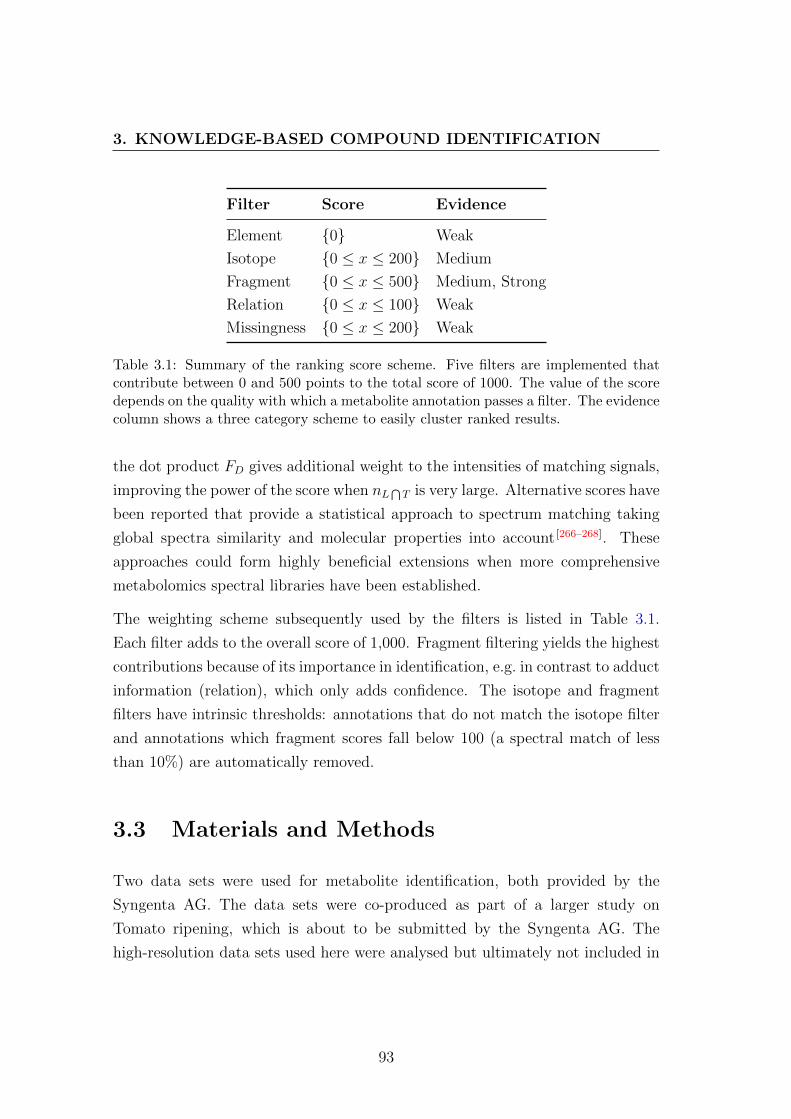
3. KNOWLEDGE-BASED COMPOUND IDENTIFICATION
Filter Score Evidence
Element {0} Weak
Isotope {0 ≤ x ≤ 200} Medium
Fragment {0 ≤ x ≤ 500} Medium, Strong
Relation {0 ≤ x ≤ 100} Weak
Missingness {0 ≤ x ≤ 200} Weak
Table 3.1: Summary of the ranking score scheme. Five filters are implemented thatcontribute between 0 and 500 points to the total score of 1000. The value of the scoredepends on the quality with which a metabolite annotation passes a filter. The evidencecolumn shows a three category scheme to easily cluster ranked results.
the dot product FD gives additional weight to the intensities of matching signals,
improving the power of the score when nL⋂
T is very large. Alternative scores have
been reported that provide a statistical approach to spectrum matching taking
global spectra similarity and molecular properties into account [266–268]. These
approaches could form highly beneficial extensions when more comprehensive
metabolomics spectral libraries have been established.
The weighting scheme subsequently used by the filters is listed in Table 3.1.
Each filter adds to the overall score of 1,000. Fragment filtering yields the highest
contributions because of its importance in identification, e.g. in contrast to adduct
information (relation), which only adds confidence. The isotope and fragment
filters have intrinsic thresholds: annotations that do not match the isotope filter
and annotations which fragment scores fall below 100 (a spectral match of less
than 10%) are automatically removed.
3.3 Materials and Methods
Two data sets were used for metabolite identification, both provided by the
Syngenta AG. The data sets were co-produced as part of a larger study on
Tomato ripening, which is about to be submitted by the Syngenta AG. The
high-resolution data sets used here were analysed but ultimately not included in
93

3. KNOWLEDGE-BASED COMPOUND IDENTIFICATION
the final manuscript. The metadata of the two studies was collected and compiled
for submission to MetaboLights [23]. The study has been submitted to Nature Sci-
entific Data: Beisken et al : Metabolic differences in ripening of wild and mutant
cultivars of Solanum lycopersicum. The following outlines the purpose and design
of the studies.
The ripening behaviour of Solanum lycopersicum and three ripening-inhibited
mutants was explored using a LC-MS2 assay. The plant material was harvested in
five to ten day intervals up to the point of flowering and daily after. Each genotype
was grown in triplicate. Each block of 52 plant samples was measured using a
group-randomization setup with interspersed quality controls: blank injections
(solvent), pooled samples (mix, see table below), and aliquots of a pooled in-
house standard tomato reference. Randomization groups were defined by day of
harvest.
The study resulted in a rich metabolic data set about the ripening behaviour of
wild type and mutant tomato. Quality measures were taken into account dur-
ing study design facilitating data analysis and enabling filtering of unintended
biological variation in the data. A total of 58 distinct reference standards were
measured on the same instrumental setup to aid metabolite identification and
consequently model validation via biological interpretation. The reference com-
pounds are those used by Syngenta for their in-house projects.
3.3.1 Tomato Cultivars
Wild type Solanum lycopersicum (Ailsa Craig, AC++) and three ripening inhib-
ited AC++ mutants were used in this study (Table 3.2): non-ripening (NOR),
ripening-inhibited (RIN), and colourless non-ripe (CNR) tomatoes [269–271]. The
plants were grown in 24 cm-diameter pots in M3 compost (Levington Horticul-
ture, Ipswich, and Suffolk, UK) and watered daily under standard greenhouse
conditions. Flowers were sampled in five to ten day intervals up to anthesis (10,
15, 20, 30, 40) and daily post-anthesis (47, 48, 49, 50, 51, 52, 53, 54). Breaker fruit
were defined as those showing the first signs of ripening-associated colour change
from green to orange. Non-ripe mutants were taken at day 49 as post-anthesis
94

3. KNOWLEDGE-BASED COMPOUND IDENTIFICATION
Name Category Description
AC++ wild type (WT) Alisa Craig variety
NOR monogenic mutant as WT except for non-ripening locus
RIN monogenic mutant ripening inhibited mutant
CNR monogenic mutant colourless non-ripe mutant
Mixed n/a pooled AC++, NOR, RIN, CNR, TomQC sample
TomQC n/a standard in-house tomato aliquots
Blank n/a blank sample with solvent
Table 3.2: Overview of sample types used in the study of different tomato cultivars. Thestudy design included four tomato cultivars: AC++, NOR, RIN, and CNR, interspersedwith pooled samples, quality control aliquots from an in-house standard tomato, andblanks consisting of solvent only.
equivalents to breaker WT fruits. All plant samples were taken at the same time
each day, frozen in liquid nitrogen, and stored at −70 ◦C until required.
3.3.2 Sample preparation
Stock standard solutions were prepared for the analytical reference standards at
a concentration of 1000 µg/mL in 20/80 HPLC analytical grade Ethanol/Water
and then diluted 10x for injection.
Tomato samples were subjected to an untargeted metabolite analysis by LC-
MS/MS of polar extracts. Approximately 30 mg of dried tomato tissue was
extracted with HPLC analytical grade Ethanol/Water 20:80. The polar extracts
were diluted 10:1 with water and injected underivatised. Samples were acquired
in three batches on 17, 20, and 21 September 2010 in positive ion mode and on
23, 24, and 27 September 2010 in negative ion mode.
3.3.3 Chromatography
All 219 samples were run on a Waters AcquityTM UPLC system (Waters Cor-
poration, USA), HSS T3 150 x 2 mm, 1.7 µm particles, UPLC column at 30 ◦C
95

3. KNOWLEDGE-BASED COMPOUND IDENTIFICATION
oven temperature. Each batch consisted of 73 samples with multiple quality
control samples. The solvents used for the assay consisted of 0.2% Formic Acid
(Solvent A) and 98/2/0.2 Acetonitrile/Water/Formic Acid (Solvent B). Gradi-
ent [time (min) / %B] starting at flow rate 0.25 mL/min: 2.5/0, 7.5/10 (flow
rate to 0.4 mL/min), 10.0/100, 12.0/100, 18.0/0, 25.0/0. Aliquots of 2 µL were
injected.
3.3.4 Mass Spectrometry
The compounds were detected using a Thermo LTQ Velos Orbitrap mass spec-
trometer operating in positive and negative Electrospray ionization (ESI) mode
at a resolution of 30,000 with a scan range from 85-900 m/z and 95-900 m/z
respectively. MS/MS spectra were obtained in a data dependent manner through
higher-energy collisional dissociation (HCD, normalized collision energy: 50.0) at
a resolution of 7,500: The two most intense mass spectral peaks detected in each
scan were fragmented to give MS2 spectra (100-900 m/z ). Full scan data was
acquired in FT (accurate mass) mode, MS/MS spectra were acquired in centroid
mode. The LTQ Velos Orbitrap used the Xcalibur control software version 2.1.0
for data acquisition. Reference standards were acquired using the same protocol
and experimental setting.
3.3.5 Reference Standards
Reference standards were commercially purchased from Fluka Analytical, Sigma-
Aldrich, and C/D/N Isotopes or prepared in-house. Pooled in-house standard
tomato reference was prepared from the shop bought Angelle variety: mashed up
in bulk and aliquoted out following the protocol outlined above.
3.3.6 Data Deposition
All samples used in this study have been submitted to MetaboLights at the Eu-
ropean Bioinformatics Institute (EMBL-EBI). Each MetaboLights entry contains
96

3. KNOWLEDGE-BASED COMPOUND IDENTIFICATION
protocols about sample collection, extraction, chromatography, mass spectrome-
try, metabolite identification, and data transformation. The study was metadata
tagged using the Investigation/Study/Assay (ISA) suite [272] in Isatab format a
tab-separated text files for experimental information. In addition, metabolites
identified and/or annotated were stored as mzTab [273] compatible tab separated
file provided as MetaboLights’s IsaCreator plug-in extension.
Data Record: Tomato Study Samples
MetaboLights’s accession MTBLS36 contains the study samples: 442 LC-MS2 files
(.mzML, 64-bit) acquired in continuous mode: 219 in positive and 223 in nega-
tive ion mode. Consistent file names are composed of <acquisitionDate> <run-
Id> <sample> <sampleTime>.
Data Record: Reference Standards
MetaboLights’s accession MTBLS38 contains the reference standards: 71 LC-MS2
files (.mzML, 64-bit) acquired in continuous mode: 43 in positive and 28 in neg-
ative ion mode. Chemical names are used as file names and linked to the ChEBI
database [274].
3.4 Data Processing and Transformation
Processing of raw data was identical for both data sets up to cross-sample fea-
ture alignment. Non-targeted LC-MS datafiles were converted to mzML format
using the program ProteoWizard [230]. Vendor-based peak picking was enabled for
MS1. The resulting mzML files were processed with MassCascade in KNIME (see
Figure 3.2 for an overview of the core workflow).
The data were time and m/z filtered before noise was reduced and features ex-
tracted with 10 ppm mass accuracy. A Durbin-Watson filter was applied with
a lenient threshold of DW = 2.8. Random signals are estimated to be around
97

3. KNOWLEDGE-BASED COMPOUND IDENTIFICATION
Fig
ure
3.2
:E
xtr
act
ofth
ep
roce
ssin
gw
ork
flow
for
met
abol
ite
iden
tifi
cati
onw
ith
Mas
sCasc
ad
ein
KN
IME
.T
he
LC
-MS
/MS
data
isre
adin
via
the
Fil
eR
eader
nod
eb
efor
eth
efe
atu
res
are
extr
acte
dfr
omth
ep
re-fi
lter
edd
ata.
Th
ed
econ
volu
ted
featu
res
are
filt
ered
for
conta
min
ants
an
dgr
oup
edin
toco
mp
oun
dsp
ectr
ath
rou
gha
cosi
ne
corr
elat
ion
matr
ix(C
osi
ne
Com
pil
er.
Isot
op
ean
dad
du
ctan
not
atio
ns
are
add
edb
efor
eth
eco
mp
oun
dsp
ectr
aar
equ
erie
dag
ain
stan
in-h
ou
sed
ata
bas
e(‘
Fea
ture
Iden
tifi
cati
on’,
not
show
n).
98

3. KNOWLEDGE-BASED COMPOUND IDENTIFICATION
Figure 3.3: Annotated correlation heatmap of tomato study features. Pearson correla-tion is indicated from red to green, [−1, 1]. Rows and columns are clustered (re-sorted).They are not ordered by their respective m/z values. Annotated features such as at[M+H]+ = 325.113 (row highlighted in blue) show strong positive correlation withtheir putatively related features. Connections are indicated with vertical blue lines.The main feature in question elutes around 90 seconds and matches multiple sugars inweb-based m/z queries, in accordance with the loss-of-Hexose and loss-of-Hexose-plus-water adduct annotations.
DW = 2. The smoothed (Savitzky-Golay, third order polynomial) features were
deconvoluted using a modified Biemann algorithm with a signal to noise ratio
of one. Common ion traces from contaminants were removed before the features
were aligned cross-sample using Obiwarp. Compound spectra were compiled from
the aligned features using a cosine correlation matrix with a correlation threshold
of ρ = 0.98. Master fragmentation spectra were compiled with a minimum signal
occurrence of two for each parent peak. Isotope and adduct annotations were
added for positive ion mode with 10 ppm mass accuracy tolerance. Figure 3.3
shows a snapshot of cross-aligned features after annotation and demonstrates the
necessity for isotope and adduct annotations to subsequently de-replicate fea-
tures, e.g. for statistical analysis [275].
99

3. KNOWLEDGE-BASED COMPOUND IDENTIFICATION
The resulting features were written out in a feature matrix after gap filling had
been applied. Unresolvable gaps were assigned a default intensity of 10,000 units.
Missingness for the matrix compilation was set to 10%. Two different sample by
feature matrices were compiled: one taking all samples and quality controls into
account (QC-Matrix), and a second matrix with samples only, i.e. NOR, RIN,
AC++, and CNR (Sample-Matrix).
Statistical analysis was carried out in the statistical programming environment
R. Pareto scaling and total signal intensity normalization were found to be op-
timal after several data pre-treatment methods were tested, preserving the data
structure while increasing the effect of small intensity features:
xij =xij − xj√
sj(3.4)
Here, x denotes the feature intensity in the sample by feature (i by j) matrix and
s represents the standard deviation. Missing values that could not be back-filled,
i.e. values with default intensity 10,000, were imputed using a 10-component
PCA model (NIPALS) before PCA was used to inspect the data and discover
trends. Observing the effect on quality control samples, total signal intensity
normalization was applied to remove batch variation and uni- and multivariate
outliers were removed. An orthogonal partial least squares (OPLS) model with
three orthogonal components was built to inspect the ripening trajectories of the
tomato cultivars – characterised by their features (X data table) – over time (Y
data table). The resulting model was subsequently used to identify features for
identification and biological interpretation.
The selected features were run against a total of four different libraries: Syn-
genta’s in-house library, KEGG, ChEBI, and PubChem Compound. These li-
braries were used in three different scenarios in order to evaluate the scoring
framework. All scenarios ran fully automated within the workflow environment.
In each scenario, annotations retrieved from the individual reference libraries
for all previously selected features were ranked to indicate the confidence in the
retrieved annotations.
Each of the three scenarios employs a different set of filters: in the first scenario
100

3. KNOWLEDGE-BASED COMPOUND IDENTIFICATION
no filter was applied. In the second scenario an isotope filter was added. In
the third scenario a fragment filter was added. Features were queried sample
by sample against the individual reference libraries before a ranked consensus
list was built from all samples (excluding control samples) with a m/z tolerance
of 10 ppm, retention time tolerance of 5 seconds, and allowed missingness of
20%. Missingness is listed as a separate filter in Table 3.1 and was applied to all
scenarios when the ranked consensus list was build.
The consensus list contained the identified metabolites ranked by an averaged
score based on the applied filters for isotope patterns, fragmentation (MS2), and
adduct information that were first applied to each sample individually. The
samples were first annotated and ranked individually to place higher emphasis
on individual samples: external effects such as noise or batch effects could distort
alignments and reduce final scores if all samples would be aligned first to generate
a feature matrix. The features in the identity table are condensed to single entries
per feature m/z value with averaged scores.
3.4.1 Known Identification
A reference library was compiled from the KEGG pathway database and com-
bined with an experimentally measured in-house library, which included retention
times of the measured standards. The KEGG library, version 57, was downloaded
in SDFile format. Disconnected structures were reduced to their largest fragment
and charged species were removed before major monoisotopic masses were calcu-
lated for query library generation. Duplicate molecule records or stereoisomers
of the same compound were removed via SMILES line notation comparison, re-
sulting in a reference library of 12,022 entries. Canonical SMILES for compari-
son were computed through the ChemAxon Marvin Extensions KNIME Feature,
2.6.3.v0135. The m/z search tolerance was set to 10 ppm. The in-house refer-
ence library contained 839 entries. The in-house library was originally measured
for metabolites relevant to plant metabolomics. The KEGG pathway database
covers core metabolic pathways.
101

3. KNOWLEDGE-BASED COMPOUND IDENTIFICATION
3.4.2 Known Unknown Identification
The PubChem database was used as reference library and queried for the target
m/z values. The PubChem database contains a range of diverse chemical com-
pounds that are mostly irrelevant for the task of metabolite identification. To
avoid the retrieval of exotic molecular structures that contain elements uncommon
in metabolites, the molecular formulas calculated for the last scenario were used
as filter for retrieved hits via PubChem’s web service. A total of 46,604 unique,
uncharged, and connected compounds were retrieved this way and compiled as
reference library.
3.4.3 Unknown Identification
Molecular formulas were generated for each feature that served as input for an
in silico structure generator (see appendix for a complete list). The molecular
formulas were generated for the selected charge-corrected feature masses with a
tolerance of 0.05 amu and checked for validity with the following rules:
• elements carbon, nitrogen, oxygen, and hydrogen only,
• element frequencies must not exceed 39 (C), 72 (H), 20 (N), and 20 (O) [240],
• compliance to the nitrogen rule [276],
• Ring Double Bond Equivalents (RDBE) values within [−0.5, 30] [248].
Sum formulas violating one or more of the rules were removed. The structure
generator Molgen [277] was run against the list of deduced sum formulas with a 30
min timeout per sum formula. To reduce computational complexity, the number
of cycles was constrained to 0-2, ring-size was limited to 0-10 atoms, and the
maximum number of structures was set to 50. Default values were used for all
other parameters. A total of 11,159 structures were generated and compiled as
reference library.
102

3. KNOWLEDGE-BASED COMPOUND IDENTIFICATION
3.5 Results
Data processing resulted in two matrices of size 219 by 211 (QC-Matrix) and 156
by 189 (Sample-Matrix). The matrices contained 292 (0.64%) and 23 (0.07%)
missing values that could not be back-filled using raw data. They were imputed
through a PCA model approach.
3.5.1 Analysis of the Quality Controls
Initial PCA on the Pareto scaled matrix shows clear batch variation in princi-
pal component 1 and 3 between samples acquired on 17.09 and 20/21.09 (Fig-
ure 3.4a). Total signal intensity normalization reduces observed batch variation
but can not eliminate it completely (Figure 3.4b). The 73 affected samples ac-
quired on 17.09 are dropped before further analysis, removing instrument induced
structure. In the PCA on the trimmed data set Tomato QC samples, blanks, and
pooled samples are each grouped together (Figure 3.4c). The biological sam-
ples are distributed along the third principal component. Expected clustering of
Tomato QC samples, blanks, and pooled samples indicate absence of additional
biological uninduced variation in the data set. Principal components 1 and 3 are
chosen because they illustrate the batch effect most dramatically. Please note,
that the homoscedasticity criteria was explored using 10 pooled samples. Slight
heteroscedasticity is notable but could not be completely removed using power
or log transformations.
3.5.2 Analysis of the Tomato Samples
Following results from the QC-Matrix, samples from 17.09 are dropped from the
Sample-Matrix, which contains the aligned features from the tomato samples.
The matrix is total signal normalized and Pareto scaled before normality of vari-
ables is explored using a skewness measure and a visual representation in the
form of quantile-quantile plots (Q-Q plots), resulting in the removal of 20 vari-
ables after inspection of the corresponding extracted mass chromatograms. Po-
103

3. KNOWLEDGE-BASED COMPOUND IDENTIFICATION
−5000
−3750
−2500
−1250
0
1250
2500
3750
5000
−20000 −13750 −7500 −1250 5000 11250 17500 23750 30000PC1
PC
3
Groups
20100917
20100920
20100921
(a) PCA: Pareto scaled QC-Matrix (acquisition date)
−20.00
−13.75
−7.50
−1.25
5.00
11.25
17.50
23.75
30.00
−70.00 −56.25 −42.50 −28.75 −15.00 −1.25 12.50 26.25 40.00PC1
PC
3
Groups
20100917
20100920
20100921
(b) As (a) plus normalization
−20
−15
−10
−5
0
5
10
15
20
−70.00 −56.25 −42.50 −28.75 −15.00 −1.25 12.50 26.25 40.00PC1
PC
3
Groups
AC.
Bla
CNR
Mix
NOR
RIN
Tom
(c) As (b) minus samples from 17.09
Figure 3.4: Overview of the tomato cultivars data set based on the QC-Matrix: All sam-ples plus blanks, Tomato QC, and pooled samples. All PCAs show the first and thirdprincipal components to illustrate batch effects. The gray circle indicates Hotelling’s T2
statistic for a 95% confidence region. (a) PCA of the Pareto scaled raw data colouredby acquisition date. Blank injections, quality controls, and samples cluster but aresmeared across the third component, exhibiting a batch effect. (b) As (a) with thedata points normalized by total signal intensity. (c) As (b) minus samples acquired on17 September with samples coloured by group.
104

3. KNOWLEDGE-BASED COMPOUND IDENTIFICATION
tential multivariate outliers are found using a PCA-based method by Filzmoser
et al. [278]. After visual inspection of the chromatographic traces, all objects are
kept. The resulting 10 component PCA model explains 50% variance (R2) in the
first two principal components with a goodness of prediction of 37% (Q2), Fig-
ure 3.5. The coefficient of determination R2 is the total ratio of variance that is
being explained by the model. The goodness of prediction Q2 results from inter-
nal seven-fold cross-validation. The applied ‘krzanowski’ type cross-validation [279]
sequentially leaves out rows (features) and columns (samples) of the input matrix
to build fold models that give loadings and scores respectively. Combinations of
these loadings and scores are then used to estimate completely left out values
(for cross-validation). The Q2 can be understood as the ratio of variance that
can be predicted independently by the model. Samples from genotypes AC++
and CNR are dominating the PCA plot. Wild type AC++ samples are spread
about the quadrants I, II, and III quadrant, whereas mutant CNR samples are
most notably in quadrants I, III, and IV. NOR and RIN samples occupy similar
space in the plot. The plot suggests that groups AC and CNR develop through
separate ways. Potential outliers indicated by the Distance to Model (DModX)
plot are kept because they do not exceed the critical threshold of twice the critical
DModX value. Because the DModX values follow a F-distribution, the critical
DModX value can derived for a significance value of 0.05 from a F-distribution
with j = 104 and i = 169 degrees of freedom.
To further investigate the data set and establish a valid model for feature selection
and metabolite identification, an orthogonal partial least squares (OPLS) model
is built (Figure 3.6). Using leave-one-out cross validation, a 1+3 model was
found to be best with a bias-corrected RMSEP of 1.95. Given the nature of
OPLS, the explained covariance between X (the Sample Matrix) and Y (sample
day) is maximized for component 1. The three dimensional OPLS plot shows the
ripening trajectories of all four genotypes. The trajectories of mutants NOR and
RIN follow a similar path. AC++ and CNR trajectories are offset and diverge
after day 30 and occupy different regions along the second and third component
respectively post-anthesis.
105

3. KNOWLEDGE-BASED COMPOUND IDENTIFICATION
−20
−15
−10
−5
0
5
10
15
20
−20.00 −13.75 −7.50 −1.25 5.00 11.25 17.50 23.75 30.00PC1
PC
2
Groups
AC.
CNR
NOR
RIN
(a) PCA: Normalized, Pareto scaled Sample-Matrix minus outliers.
0.0
0.1
0.2
0.3
0.4
0.5
0.6
0.7
0.8
0.9
1.0
0 1 2 3 4 5 6 7 8 9 10 11Component
Val
ue
Statistic
Q2
R2
(b) Goodness of fit and prediction
0.0
0.5
1.0
1.5
2.0
2.5
3.0
1 11 21 31 41 51 61 71 81 91 101Observation
Dis
tanc
e to
Mod
el
(c) Distance to Model plot
Figure 3.5: Final PCA model for the tomato cultivars data set. (a) PCA of the nor-malized and Pareto scaled Sample-Matrix: Genotype samples only. The samples arecoloured by genotype. The gray circle indicates Hotelling’s T2 statistic for a 95% con-fidence region. Wild type AC++ samples are spread about the quadrants I, II, and IIIquadrant, whereas mutant CNR samples are most notably in quadrants I, III, and IV.NOR and RIN samples occupy similar space in the plot. (b) Cumulative plot for thegoodness of fit (R2) and prediction (Q2). (c) Distance to Model plot with a criticalvalue threshold for potential outliers of 1.29866 (green line) and twice the critical valuethreshold for definitive outliers (red line).
106

3. KNOWLEDGE-BASED COMPOUND IDENTIFICATION
(a) OPLS: Genotype time trends (comp 1,2)
(b) OPLS: Genotype time trends (comp 1,3)
Figure 3.6: OPLS model for the tomato cultivars data set. Score plots for the firstvs. second (a) and first vs. third (b) component are shown with a trendline approxi-mated via LOESS. The samples are coloured by genotype and labelled by sample date.Covariance is maximized between the Sample-Matrix and the sample day in the firstcomponent. The trajectories of mutants NOR and RIN follow a similar path. AC++
and CNR trajectories are offset and diverge after day 30 and occupy different regionsalong the second and third component respectively after flowering at day 47.
107

3. KNOWLEDGE-BASED COMPOUND IDENTIFICATION
Observations of mutant CNR spread significantly more than observations of wild
type AC++. Subsequently separate OPLS models are built vs. time for each
genotype to identify biologically relevant targets for metabolite identification.
OPLS is chosen over OPLS-DA (discriminant analysis) because of familiarity
with OPLS and its availability in the R environment. OPLS-DA is an extension
of the OPLS technique that takes class information into account. In general, it
is more suitable for discrimination modelling. Loadings of the first component
of each AC++ - mutant pair are plotted to single out up- and down- regulated
metabolites as identified by the models. The first component encrypts Y – the
sample time – and is thus most revealing for metabolites that change over time
(Figure 3.7). Metabolites below the first quartile of the distribution of AC++ and
above the third quartile of the distribution of a mutant (or vice versa) are chosen
for identification because they exhibit maximum change over time in multivariate
space. That is, metabolites occupying the extreme ends of the wild type and
mutant distributions are chosen so that they have high loading values in one
genotype and low loading values in the other. This procedure results in 13, 2,
and 2 singled out features for AC++ - CNR, AC++ - NOR and AC++ - RIN
models.
3.5.3 Identification
A total of 13 unique features were singled out using the OPLS loadings plot
approach. Missingness and element filters were included by default every time.
They defined the baseline score of 160 for a missingness of 20%.
Known Identification
A total of 18 hits, i.e. distinct molecules, were returned. Grouped by feature, only
six features had metabolite annotations. For those 18 hits, four had retention time
information from the in-house library: valine, betaine, pidolic acid, and citrulline.
With the exception of betaine, retention times matched within four seconds. Lists
of annotations of individual features are shown in the representative Tables 3.3,
108

3. KNOWLEDGE-BASED COMPOUND IDENTIFICATION
(a) Loadings comp. 1: AC++ vs CNR
(b) Loadings comp. 1: AC++ vs NOR (c) Loadings comp. 1: AC++ vs RIN
Figure 3.7: The pairwise loadings of the first component of the individual genotypeOPLS models is shown for (a) AC++ vs CNR, (b) AC++ vs NOR, and (c) AC++
vs RIN. Metabolites that do not change over time center around (0,0). The dashedblue line indicates the diagonal along which metabolite intensities increase or decreasetogether. Metabolites below the first quartile of the distribution of AC++ and above thethird quartile of the distribution of a mutant (or vice versa) are chosen for identificationand are highlighted in red. That is, metabolites occupying the extreme ends of the wildtype and mutant distributions are chosen so that they have high loading values in onegenotype and low loading values in the other.
109

3. KNOWLEDGE-BASED COMPOUND IDENTIFICATION
Name Depiction Score
Frag. Isotope None
pidolic acid†* 554 455 160
1-pyrroline-3-hydroxy-5-carboxylate
554 455 160
4-oxoproline 552 455 160
MS2 spectrum
Table 3.3: Metabolite annotations for m/z 130.05 with cumulative scores for no, isotope,and fragment filtering. Missingness and element filters were always included. Thecalculated score ranks 4-oxoproline lower. All structures are highly similar. †Theextracted MS2 spectrum shown is dominated by a peak at 84.044 (putative structureshown). *Matching retention time in the in-house library at 275 seconds.
3.4, and 3.5. The remaining three tables are in the appendix. The tables list the
scores for the three additive filters. Where present, an extracted MS2 spectrum
is shown with its dominant peak annotated with a putative fragment.
The scoring framework adds discriminatory power to the ranking of metabolite
annotations. The missingness and element filter set a start score of 160; the
score increases if a suitable isotopic envelope is present. It increases further in
the presence of MS2 spectra if fragmentation signals match. The discriminatory
power lies solely within the fragmentation filter. All compounds are very similar
to each other. Their theoretical isotopic abundances fit the measured isotope
signals and their fragmentation spectra are dominated by few signals those m/z
110

3. KNOWLEDGE-BASED COMPOUND IDENTIFICATION
values match multiple charged fragmented substructures of each of the putative
compounds. Retention time from the in-house library is the only factor that can
potentially differentiate identically ranked compounds. However, only four hits
from the KEGG database also had associated retention times in the in-house
library. For increased confidence, all annotations would need associated retention
times to enable comparisons. Betaine (Table 3.5) is the only example of a lower-
ranked compound with a differing retention time.
Name Depiction Score
Frag. Isotope None
asparagine† 351 209 160
3-ureido-propionate
350 209 160
glycylglycine 350 209 160
N-carbamoyl-sarcosine
325 209 160
MS2 spectrum
Table 3.4: Metabolite annotations for m/z 133.061 with cumulative scores for no,isotope, and fragment filtering. Missingness and element filters were always included.The calculated score singles out asparagine. All structures are highly similar. †Theextracted MS2 spectrum shown at the bottom of the table is dominated by a peak at87.055 (putative structure shown).
111

3. KNOWLEDGE-BASED COMPOUND IDENTIFICATION
Name Depiction Score
Frag. Isotope None
valine†* 559 359 160
D-norvaline 559 359 160
2-amino-2-methylbutanoate
559 359 160
4-methyl-aminobutyrate
559 359 160
amyl nitrite 559 359 160
5-amino-pentanoate
557 359 160
betaine 557 359 160
MS2 spectrum
Table 3.5: Metabolite annotations for m/z 118.086 with cumulative scores for no,isotope, and fragment filtering. Missingness and element filters were always included.The calculated score does not allow for selective ranking among the five best structures.With exception of the charged compound betaine, all structures are highly similar. †Theextracted MS2 spectrum shown at the bottom of the table is dominated by its parentpeak (putative structure shown). *Matching retention time information in the in-houselibrary at 154 seconds.
112

3. KNOWLEDGE-BASED COMPOUND IDENTIFICATION
Known Unknown Identification
A total of 261 molecular formulas were generated. Feature 327.117 was elimi-
nated from this scenario at the beginning because the putatively correct molec-
ular formula C14H18N2O7 was missed by the formula generator. Other formulas
calculated for the same feature were removed by the isotope filter because they
did not match the measured isotope pattern.
For known unknowns, i.e. hits from a generic compound database like PubChem
Compound, the framework helps to narrow down the annotation space from sev-
eral to a few hundred annotations but is unable to single out one compound
(Table 3.6). The table lists the rank of the selected metabolite annotations from
the ‘Known Identification’ scenario within the retrieved compound lists. The
compound lists were grouped by score. The fraction of hits with identical scores
to all hits is also listed, i.e. the number of matching references up to the group
that contains the annotation divided by all matching references. For example,
feature 118.086 is thought to represent valine based on the ‘Known Identifica-
tion’ scenario (Table 3.5). Valine is in the highest ranked group of PubChem
Compound retrievals (Rank 1 ), which includes 45% of all matching retrievals
from PubChem Compound for that particular feature. The scoring framework
eliminates 55% of matching compounds.
The scores are identical for all filters if the best scores from the PubChem Com-
pound retrievals are compared to the scores from the previous scenario. Up to the
isotope filter, this is to be expected because the missingness value and molecular-
formula based theoretical isotopic abundances are identical. The highest ranked
compounds have identical molecular formulas.
The only discriminating factor remaining is the fragmentation score. The score
is also identical for all cases except for feature 197.096, which was ranked fourth:
the best fragmentation score is larger by one unit. Given the information from the
data, PubChem does not offer better matching compounds but a list of equally
well matching compounds.
113

3. KNOWLEDGE-BASED COMPOUND IDENTIFICATION
m/z Rank Fraction Score (PubChem/KEGG)
Frag. Isotope None
118.086 1 45% 559/559 359/359 160/160
130.05 1 68% 554/554 455/455 160/160
133.061 1 81% 350/350 209/209 160/160
176.103 1 100% n/a 260/260 160/160
197.096 4 72% 370/369 251/251 160/160
327.117 n/a n/a n/a n/a 160/160
Table 3.6: For the selected features (m/z ), the rank of the group that contains thefeature’s annotation is shown and the fraction of the number of all molecules withinor up to that group in relation to all retrieved hits for that feature. The top-listedannotations from the ‘Known Identification’ scenario were used for ranking. The scorecompares the best score of all retrieved annotations for a feature to the ‘Known Identifi-cation’ scenario. They are identical with exception of feature 197.0.96. Feature 327.117did not yield the required molecular formula during the automated process.
Unknown Unknown Identification
The calculated average score of matching annotations is expected to be worse for
the Molgen library, i.e. lower, than the average score from the ‘Known Identifi-
cation’ scenario because chemical space is traversed at random.
Table 3.7 compares the best hits retrieved from the Molgen library versus previ-
ously retrieved best hits. With exception of feature 197.096, the fragmentation
scores from the Molgen library are worse for all features where fragmentation
spectra exist.
Feature 197.096 matches carbon-rich structures with few hetereoatoms that give
similar fragments if fragmented deterministically. The isotope score contributions
are identical for both scenarios because identical molecular formulas resulted in
the best overall score.
114

3. KNOWLEDGE-BASED COMPOUND IDENTIFICATION
Mol. Formula m/z Depiction Score (Molgen/KEGG)
Frag. Isotope None
C5H11NO2 118.086 557/559 359/359 160/160
C5H7NO3 130.05 553/554 455/455 160/160
C4H8N2O3 133.061 343/351 209/209 160/160
C6H13N3O3 176.103 n/a 260/260 160/160
C14H12O 197.096 369/369 251/251 160/160
Table 3.7: Scored metabolite annotations for the best hits in the Molgen library versusthe best hits in the KEGG library for five selected ion traces. Cumulative scores forno, isotope, and fragment filtering are shown with Molgen/KEGG scores. Missingnessand element filters give a base score of 160. With the exception of feature 197.096,fragmentation scores from the ‘Known Identification’ scenario are greater than scoresfrom the Molgen library.
Feature Analysis
Putative feature identifications were further investigated through biological in-
terpretation based on univariate statistics. Feature abundances across samples,
their distributions, and receiver-operator characteristic (ROC) curves were com-
piled for every genotype.
The feature abundances shown in the scatterplots are sorted by genotype and har-
vest date in ascending order. The trend for the features’ abundances is indicated
through locally weighted scatterplot smoothing. Boxplots show the median (mid-
dle line) and lower (25%) and upper (75%) percentiles of the abundances.
115

3. KNOWLEDGE-BASED COMPOUND IDENTIFICATION
The ROC curves describe the power of the respective features for binary classifi-
cation of either of the three mutant genotypes (RIN, NOR, CNR) versus the wild
type AC++. This statistic supplements the boxplots, indicating how characteris-
tic the total change of a feature is for a genotype compared to AC++.
A complete list of univariate feature statistics for all 13 unique features extracted
from the OPLS loading plots can be found in the appendix, including Pearson’s
correlation matrices for each genotype. Here, the six features that have annota-
tions are discussed because of biological interpretability.
Figure 3.8a summarizes feature 118.086. The relative abundances decline dur-
ing the ripening period in all genotypes. The distributions are similar and the
feature does not appear to have discriminatory power in univariate space. The
importance assigned by the OPLS loadings plot between AC++ and CNR is not
reflected.
Feature 130.05 shows a distinct difference between the AC++/CNR and NOR/RIN
genotypes (Figure 3.8b). The feature abundances are not decreasing over time to
the extend of the wild type and colorless non-ripe feature abundances as indicated
by the trend lines.
In Figure 3.9a, AC++’s level of feature 133.061 rises quicker over time than for the
other genotypes. The overall difference is minor and does not impact significantly
on the ROC curve. The differing behaviour is captured in the OPLS loading plots:
in all three comparisons, the loadings do not indicate correlation.
Feature 176.103 (Figure 3.9b) dramatically drops in abundance for CNR, dis-
tinguishing CNR from the wild type. In Figure 3.10a and 3.10b, the levels of
features 197.096 and 327.118 are spiking compared to the other genotypes.
116

3. KNOWLEDGE-BASED COMPOUND IDENTIFICATION
−20
−15
−10
−5
0
5
10
15
20
0 15 30 45 60 75 90 105Sample Number
Rel
ativ
e A
bund
ance
m/z: 118.086 AC++ CNR NOR RIN
−20
−15
−10
−5
0
5
10
15
20
AC++ CNR NOR RINGenotype
Rel
ativ
e A
bund
ance
0.00
0.25
0.50
0.75
1.00
0.00 0.25 0.50 0.75 1.00False positive rate
True
pos
itive
rat
e
(a) Univariate statistics for feature 118.086
−30.00
−23.75
−17.50
−11.25
−5.00
1.25
7.50
13.75
20.00
0 15 30 45 60 75 90 105Sample Number
Rel
ativ
e A
bund
ance
m/z: 130.05 AC++ CNR NOR RIN
−30.00
−23.75
−17.50
−11.25
−5.00
1.25
7.50
13.75
20.00
AC++ CNR NOR RINGenotype
Rel
ativ
e A
bund
ance
0.00
0.25
0.50
0.75
1.00
0.00 0.25 0.50 0.75 1.00False positive rate
True
pos
itive
rat
e
(b) Univariate statistics for feature 130.05
Figure 3.8: Univariate statistics for features 118.086 (a) and 130.05 (b). The scatterplotshows feature abundances grouped by genotype and sorted by harvest date in ascend-ing order with applied locally weighted smoothing. The boxplots display the median(middle line) and lower (25%) and upper (75%) percentiles of the abundances. TheROC curves indicate the binary classification power of the mutant genotypes versusthe wild type AC++.
117

3. KNOWLEDGE-BASED COMPOUND IDENTIFICATION
−20
−15
−10
−5
0
5
10
15
20
0 15 30 45 60 75 90 105Sample Number
Rel
ativ
e A
bund
ance
m/z: 133.061 AC++ CNR NOR RIN
−20
−15
−10
−5
0
5
10
15
20
AC++ CNR NOR RINGenotype
Rel
ativ
e A
bund
ance
0.00
0.25
0.50
0.75
1.00
0.00 0.25 0.50 0.75 1.00False positive rate
True
pos
itive
rat
e(a) Univariate statistics for feature 133.061
−9−8−7−6−5−4−3−2−1
0123456789
10
0 15 30 45 60 75 90 105Sample Number
Rel
ativ
e A
bund
ance
m/z: 176.103 AC++ CNR NOR RIN
−9
−8
−7
−6
−5
−4
−3
−2
−1
0
1
2
3
4
5
6
7
8
9
10
AC++ CNR NOR RINGenotype
Rel
ativ
e A
bund
ance
0.00
0.25
0.50
0.75
1.00
0.00 0.25 0.50 0.75 1.00False positive rate
True
pos
itive
rat
e
(b) Univariate statistics for feature 176.103
Figure 3.9: Univariate statistics for features 133.061 (a) and 176.103 (b). The scat-terplot shows feature abundances grouped by genotype and sorted by harvest date inascending order with applied locally weighted smoothing. The boxplots display themedian (middle line) and lower (25%) and upper (75%) percentiles of the abundances.The ROC curves indicate the binary classification power of the mutant genotypes versusthe wild type AC++.
118
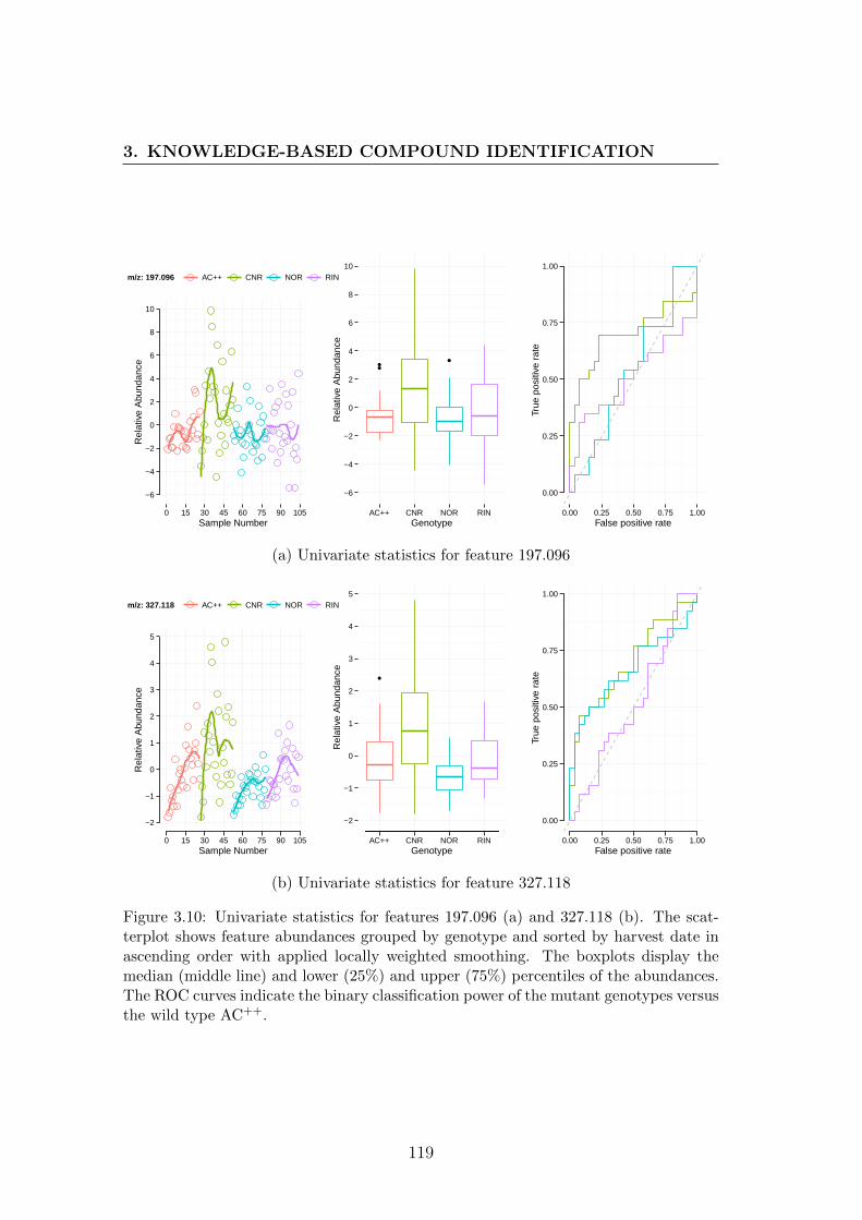
3. KNOWLEDGE-BASED COMPOUND IDENTIFICATION
−6
−4
−2
0
2
4
6
8
10
0 15 30 45 60 75 90 105Sample Number
Rel
ativ
e A
bund
ance
m/z: 197.096 AC++ CNR NOR RIN
−6
−4
−2
0
2
4
6
8
10
AC++ CNR NOR RINGenotype
Rel
ativ
e A
bund
ance
0.00
0.25
0.50
0.75
1.00
0.00 0.25 0.50 0.75 1.00False positive rate
True
pos
itive
rat
e
(a) Univariate statistics for feature 197.096
−2
−1
0
1
2
3
4
5
0 15 30 45 60 75 90 105Sample Number
Rel
ativ
e A
bund
ance
m/z: 327.118 AC++ CNR NOR RIN
−2
−1
0
1
2
3
4
5
AC++ CNR NOR RINGenotype
Rel
ativ
e A
bund
ance
0.00
0.25
0.50
0.75
1.00
0.00 0.25 0.50 0.75 1.00False positive rate
True
pos
itive
rat
e
(b) Univariate statistics for feature 327.118
Figure 3.10: Univariate statistics for features 197.096 (a) and 327.118 (b). The scat-terplot shows feature abundances grouped by genotype and sorted by harvest date inascending order with applied locally weighted smoothing. The boxplots display themedian (middle line) and lower (25%) and upper (75%) percentiles of the abundances.The ROC curves indicate the binary classification power of the mutant genotypes versusthe wild type AC++.
119

3. KNOWLEDGE-BASED COMPOUND IDENTIFICATION
3.6 Discussion
Thirteen features were selected for identification that were believed to be con-
tributing to differences in ripening between the investigated genotypes. Three
scenarios were applied to test the scoring framework. Score contributions from
the missingness, adduct, and isotope filters added little discriminatory power
to the ranking. These filters primarily ensured that highly unlikely compound
annotations were removed from the beginning.
The remaining list of similar compounds, i.e. identical molecular formulas and
presence/absence of cycles, still comprised hundreds of entries for the ‘Known
Unknown’ scenario (using the PubChem Compound database) that could not
be trimmed down further using fragmentation information. This can partially
be explained by poor fragmentation behaviour of the measured ions, e.g. due to
insufficient fragmentation optimization in the instrument, and deficiencies that
result from a deterministic structure fragmentation approach that traverses all
possible fragments without physical constraints to rank and discard unlikely frag-
ments.
For the smaller, biologically relevant database used in the ‘Known Identification’
scenario, the score contribution from the fragmentation filter allowed the discrim-
ination of similar retrieved hits highlighting a single or a few compounds. The
score differences are small but reflect the absence of explainable fragmentation
signals that are important for identification. Currently, the structure fragmenta-
tion tool, which is used in the fragmentation filter, does not predict abundances
of fragments. It only generates fragments and abundances are set to one. Because
the fragmentation filter calculates a score based on the match of the predicted
to the measured fragmentation spectrum that takes abundances into account, a
more elaborate fragmentation tool that also predicts abundances is likely to in-
crease the scoring differences seen. This is exemplified in the ‘Unknown Unknown
Identification’ scenario. If chemical compounds for annotations were computed
randomly, the scores of the best matching annotations were smaller than for the
relevant annotations from the ‘Known Identification’ scenario.
120

3. KNOWLEDGE-BASED COMPOUND IDENTIFICATION
To consolidate the ranked feature annotations and demonstrate correct data pro-
cessing and identification by MassCascade, univariate analysis was carried out.
The features were initially selected based on a multivariate OPLS approach. Be-
cause univariate statistics do not capture co-linearity between variables, not all
features appear to be of importance in their univariate evaluation. The wild
type AC++ and the mutant genotypes CNR, NOR, and RIN have been shown to
share the same compounds but that their concentrations vary during ripening,
resulting in the different trajectories captured in Figure 3.6 [280]. RIN and NOR
mutants never achieve a ripe stage, i.e. their ripening stops before maturity. This
behaviour is also captured in their metabolic profile as can be seen by the OPLS
plot and in the abundances of feature 130.05 (Figure 3.8b), where pidolic acid has
been reported to be closely correlated to ripening [281]. Asparagine concentrations,
feature 133.061 (Figure 3.9a), have been reported to increase during ripening [280]
(major N form in plants), whereas valine concentrations, feature 118.086 (Fig-
ure 3.8a), have been reported to decrease during ripening [282,283]. Citrulline is
closely linked to its precursor arginine, which is regarded as plant growth regulator
in the greater network of polyamine-mediated effects [284], potentially explaining
its complete defect in the CNR genotype. The discussed features identifications
and extracted abundances appear to be reasonable within the outlined biological
context.
3.7 Conclusion
Knowledge-based compound identification can help to reduce the size of lists
of putative metabolite annotations in metabolomics studies. The implemented
approach of information aggregation followed by scoring and ranking based on
adduct, isotope, and fragmentation data helps to discard biologically irrelevant
structures as can be seen in the example scenarios. Annotations could be removed
after initial m/z -based assignment.
Similar structures retrieved from compound databases are more difficult to dif-
ferentiate based on mass spectrometry data alone as demonstrated in the next
121

3. KNOWLEDGE-BASED COMPOUND IDENTIFICATION
section – unless multiple MSn are recorded, a currently infeasible approach for
untargeted studies. As the ‘Known Identification’ scenario indicates, poor frag-
mentation behaviour – due to low ionisation efficiency – and low m/z values
render discrimination, e.g. between valine/norvaline or pidolic acid/1-pyrroline-
3-hydroxy-5-carboxylate impossible. Confidence in metabolite rankings can be
increased by addition of retention time (or retention index) information. How-
ever, this approach is limited by the poor ratio of the maximum feasible size of
any measured in-house library versus the tangible metabolite space. In general,
the addition of orthogonal sources of information increases the ability to rank
putative metabolite annotations.
The study design, data, and processing/analysis processes are captured using
open tools to achieve maximum transparency and reproducibility in line with cur-
rent community-wide efforts in metabolomics. To that end, the complete study
including the in-house library has been deposited in the MetaboLights database
and a Scientific Data article was submitted to the Nature publishing group. The
strength of MassCascade, introduced in chapter 2.1, has been demonstrated by
using it for data processing and analysis including metabolite annotation and
ranking. The created workflow that was used throughout the analysis process is
available online, can easily be shared, and includes all set parameters. Its inte-
gration into the workflow environment KNIME enabled additional functionality,
such as the dereplication of features or the required data transformation for the
compilation of reference libraries. Open data or the formation of a ‘Datument’
has been thoroughly achieved.
Outstanding problems involve the generation of rational fragmentation spectra in
silico that also give predicted signal abundances. This will significantly increase
the power of the scoring framework for annotations from highly similar molecular
species.
122

3. KNOWLEDGE-BASED COMPOUND IDENTIFICATION
3.8 Technical Validation
The identification framework implemented in MassCascade – previously applied
to the analysis of the tomato samples – is validated against a publicly avail-
able benchmark data set to further consolidate the methodology. The C ritical
Assessment of Small M olecule I dentification (CASMI) is an inaugural open con-
test based on a common open dataset to evaluate identification methods for LC-
or GC-MS data. CASMI was founded by Emma L. Schymanski and Steffen Neu-
mann in 2012 and is at the time of writing in its third round (2014) [285].
Test data has been taken from the CASMI contest in 2013 for which the challenge
data and the solutions are available online (http://www.casmi-contest.org/
2013/). For a comprehensive description of the data format, ranking procedures,
and structure of the contest, please see the article by Schymanski et al. [286].
A total of 11 out of 16 challenges are selected from category 2 (best structure
identification). The missing five challenges are centred around data acquired in
negative ion mode, currently not fully supported by the identification framework
in automated mode. ‘Automatic method’ is a boolean flag in the CASMI contest
indicating whether the metabolite identification process has run without man-
ual intervention, the scenario chosen for this technical validation. Category 1
(best molecular formula) has been skipped because it is an inherent part of cat-
egory 2. Following CASMI reporting standards, details per challenge are listed
in Table 3.8. For details on the individual rankings, please see Schymanski et
al. [286].
3.8.1 Methods
Test data is provided as peak lists in flat files. Each challenge contains one peak
list for MS and a separate peak list for MS/MS. No raw data or chromatographic
profiles are provided. The accompanying meta files contain the instrumental
parameters plus a brief description of the challenge including tips such as ‘contains
aromatic structures’ or ‘contains amide bonds’.
123

3. KNOWLEDGE-BASED COMPOUND IDENTIFICATION
For each challenge, both MS and MS/MS peak lists are converted to MassCas-
cade Features and aggregated in a Feature Set. Fragmentation spectra are linked
to their parent peaks either through information provided in the respective meta
files or through manual evaluation of the MS and MS/MS spectra. The gener-
ated Feature Sets serve as starting point for the annotation and identification
process.
Adduct and isotope annotations are calculated using a 10 ppm m/z tolerance
window before the PubChem Compound database is queried through the Chem-
Spider web service for putative structures for the parent peak in MS1. Simulta-
neously, the MS and MS/MS spectra are queried against MassBank with default
parameters. Mass accuracies were adjusted between 3 and 10 ppm guided by the
challenge meta files. Retrieved metabolite annotations are submitted to brute-
force feature fragmentation and MS/MS assignment before candidate ranking is
carried out using all score filters (default parameters).
MassBank spectra deposited by ’CASMI2013 organizers’ are ignored in this exer-
cise. Otherwise, in the case of matching MassBank MS/MS spectra, the fragmen-
tation filter’s score is replaced by half of the score of MassBank’s query score for
the fragmentation spectrum, ensuring that both scores are comparable. Ranked
candidates are further filtered using a SMARTS substructure search based on the
challenge tips that describe structural properties of the correct solution.
3.8.2 Results & Discussion
Parsing and formatting the plain data files were the most time-consuming steps.
The annotation and identification workflow ran fully automated after initial set-
up and deduction of the SMARTS query strings for each challenge. The Chem-
Spider and MassBank web services were reliable but slow in execution. Preference
was given to queries against MassBank over Pubchem Compound because Mass-
Bank is an experimental mass spectral database and thus able to provide better
confidence in putative metabolite annotations.
A total of one MS spectrum with a single associated MS/MS spectrum was gen-
124

3. KNOWLEDGE-BASED COMPOUND IDENTIFICATION
# rank tc bc wc ec rrp p wbc wwc wec wrrp
1 7 2954 0 2947 7 1.00 0.00 0.00 0.99 0.01 0.99
2 1 1278 0 1277 1 1.00 0.00 0.00 1.00 0.00 1.00
4 226 323 0 90 226 0.65 0.00 0.00 0.08 0.92 0.08
5 1 237 0 236 1 1.00 0.00 0.00 1.00 0.00 1.00
7 22 44 0 22 22 0.76 0.04 0.00 0.26 0.86 0.14
8 3 17 0 14 3 0.94 0.14 0.00 0.58 0.42 0.58
9 1 63 0 62 1 1.00 0.02 0.00 0.98 0.02 0.98
10 6 18 1 12 5 0.82 0.12 0.12 0.31 0.58 0.31
13 366 384 0 18 366 0.52 0.00 0.00 0.01 0.99 0.01
14 997 3457 0 2460 997 0.86 0.00 0.00 0.36 0.49 0.51
16 – 1879 – – – – – – – – –
Table 3.8: Results of the technical validation using the CASMI data set of 2013. Resultsare reported following the CASMI reporting standards: #, challenge; rank, absoluterank of correct solution; tc, total number of candidates; bc, number of candidates witha score better than correct solution; wc, number of candidates with a score worse thancorrect solution; ec, number of candidates with same score as the correct solution; rrp,relative ranking position (1.0 is good, 0.0 is not); p, score of correct solution; wbc, sumof scores better than correct solution; wwc, sum of scores worse than correct solution;wec, sum of scores equal to correct solution; wrrp, RRP weighted by the scores (1 isgood).
erated for each challenge. The result of the analyses is summarised in Table 3.8.
Note that challenges 3, 6, 11, 12, and 15 are missing because of issues around the
negative ion mode as explained in the preceding section. Because the filters it-
eratively remove irrelevant candidates, e.g. disconnected structures or structures
that do not match measured isotopic envelopes, and do not report complete lists
of all candidates, removed candidate entries were given a base score of 200 in
order to calculate the normalised scores (p, wbc, wwc, wec, and wrrp) through
the total sum of scores as described by Schymanski et al. [286]. The base score
reflects the score that any candidate would be given by default if it passed the
missingness filter. This can be assumed in this exercise because the data reflects
extracted features of interest.
Similar to other contestants of the CASMI challenge, we used MassBank and Pub-
125

3. KNOWLEDGE-BASED COMPOUND IDENTIFICATION
Chem Compound as query databases to retrieve collections of metabolite struc-
tures as starting point. The results table shows that the identification framework
was able to extract the correct structures from larger sets (up to 3, 500) and rank
them within the top 10 candidate structures in 6 out of 11 cases. The correct
candidate structure was ranked lower in challenges #7 (rank 22), #4 (rank 226),
#13 (rank 366), and #14 (rank 997). The correct solution was not found at all
in challenge #16.
The solution to challenge #7 is a pentameric proanthocyanidin (Cinnamtannin
A3). Similar structures such as other flavanol-based compounds could not be
differentiated from the correct solution due to the repetitive nature of polymeric
compounds, resulting in 22 equal ranked candidates. In challenges #4, #13 and
#14, the high rank also results from limitations of the framework to differentiate
very similar molecular structures, resulting in 226, 366 and 997 equal ranked
candidates. In challenge #16 the correct structure was removed by the isotope
filter: the measured isotopic peak ([M + 1]+) did not fit the value calculated by
the program.
Overall, an evaluation of the absence of better candidates in all but one challenge
combined with the large numbers of equal ranked candidate structures, indicates
the difficulty in metabolite identification using mass spectrometry data alone.
Whereas – with regard to the CASMI contest – the framework’s performance
resides between the (semi-)automated methods of the contestants ES and FA (re-
sults of the contest are available on the official website), the framework performed
poorly compared to the contestants who used more manual methods of investi-
gation and took additional information into account such as species, retention
times, and classifications such as ’natural product’.
126

CHAPTER 4
Computational Workflows for
Cheminformatics
4.1 Introduction
The routine work of a cheminformatician involves the processing of collections
of small molecules. Standardising molecules, e.g. adding hydrogens or removing
unconnected structures, calculation of molecular descriptors, and visualisation of
chemical structures in two- or three-dimensional space are just a few examples of
recurring tasks that are carried out upstream of cheminformatic pipelines. Several
free and open source cheminformatics libraries and tools have been developed to
deal with these tasks, such as the CDK [287], RDKit [191], and OpenBabel [193].
Building a comprehensive pipeline for handling small molecules requires a basic
understanding of a scripting language to concatenate input and output from
different tools or call functions from a cheminformatics library. For experimental
scientists, usage of APIs (application programming interfaces) or programming
languages can add a constraint to more in-depth analysis. Standalone tools suffer
from limited scope, i.e. they mostly do one thing only. Even simple tasks like the
visual characterisation of a chemical library [288] require importing and exporting
127

4. WORKFLOWS FOR CHEMINFORMATICS
of data in various formats using different tools. This poses challenges related to
the maintainability and modularity of custom pipelines that are created for these
tasks.
Workflow environments circumvent the above mentioned challenges to various
degrees by providing a common platform for different tools and have become
popular with the science community [289]. A cheminformatics plug-in, KNIME-
CDK, has been developed based on the Chemistry Development Kit (CDK),
an open-source cheminformatics library. It wraps elements of the library’s core
functionality and exposes it to the user. In contrast to other cheminformatics
plug-ins available in KNIME, the project and its core library are fully open and
community-driven.
KNIME-CDK is part of KNIME’s community contributions and adheres to their
software versioning system. Separate versions exist for the major KNIME re-
leases, 2.7, 2.8, and 2.9, and for the nightly version for active development.
KNIME-CDK is an official ‘Trusted Community Contributions’ since version
2.9.
4.2 KNIME-CDK’s Implementation
KNIME-CDK has been developed in Java R© 1.6 for the KNIME legacy version
2.6 and Java R© 1.7 for all KNIME versions greater than 2.6. Following KNIME’s
data model, individual CDK molecule representations are stored in their own
data cell type, the atomic unit for tabular data transfer from one node to an-
other. Community cheminformatics plug-ins come with their own cell types that
uniquely capture the underlying library’s molecule representations. To make data
cell types of other cheminformatics plug-ins accessible without explicit conversion
on the code level, generic KNIME chemistry types are used as buffer in between
cheminformatics plug-ins. Thus, KNIME-CDK depends on the generic KNIME
chemistry types that serve as a wrapper for common chemistry file formats (see
section 1.2.2).
128

4. WORKFLOWS FOR CHEMINFORMATICS
(a) Plug-in architecture (b) KNIME-CDK node model
Figure 4.1: Overview of the KNIME-CDK architecture and node model. (a) The plug-in forms part of the KNIME Desktop and serves as an interface between the CDKcore library for data processing, JChemPaint for chemical drawing, and Jmol for 3Dvisualisation. (b) The node model enables molecular compounds from any genericchemistry format to be processed within the KNIME-CDK environment. A compoundfrom the RDKit cheminformatics package is processed in CDK (logP calculation) beforeit is further used for a web query that does not form part of the CDK plug-in.
4.2.1 Structure
The KNIME-CDK plug-in follows the classical KNIME node architecture as de-
scribed in section 1.2.4. Nodes run within Java’s R© concurrency framework [229]
with threading enabled for fast execution. KNIME-CDK uses CDK for data pro-
cessing and visualisation, JChemPaint [290] for chemical drawing, and Jmol [291]
for visualisation in 3D space (Figure 4.1a). No direct file input or output nodes
exist. Instead, KNIME tables become usable within the KNIME-CDK environ-
ment after chemistry cell type conversion from a generic format to the internal
KNIME-CDK representation (Figure 4.1b).
4.2.2 Persistence
Data persistence is guaranteed via the Chemical Markup Language (CML) [207]
serializing the molecule when necessary. The underlying CDK molecules are han-
dled and stored within data cells in standardized form, i.e. with implicit hydrogen
atoms added, atom types perceived, and aromaticity detected. This guarantees
129

4. WORKFLOWS FOR CHEMINFORMATICS
consistency across all nodes and simplifies usability of the plug-in by automating
technical details from the user, hence allowing the scientist to focus on the task
at hand.
The nightly build features persistence via the line notation SMILES based on
a recent release of CDK version 1.5.4. In contrast to CML, SMILES – as line
notation system – does not allow for additional information to be stored directly.
Consequently, atom types and aromaticity are perceived every time a molecule
is requested for processing, i.e. at every node. This overhead is balanced out
by advantages of the SMILES system: information density and applicability
within the workflow environment. Two- and three-dimensional coordinates as
well as additional information about substructure highlights (see section 4.3.3)
are stored in vectorised form with the SMILES notations. It should be noted that
a non-canonical version of SMILES is used to increase execution speed: isomeric
SMILES. However, conversion rounds of SMILES to native CDK representation
to SMILES always result in the same SMILES and native CDK representation
because the atom order is preserved in a separate auxiliary array. The array
maps the order of the atoms in the CDK representation to the order in which
the SMILES string is parsed. SMILES and auxiliary information are serialized
to disk in a byte stream.
4.3 KNIME-CDK’s Functionality
The plug-in includes methods for the generation of two- and three-dimensional
coordinates, atom signatures, common fingerprints, e.g. MACCS and Pubchem
Compound, two- and three-dimensional molecular descriptor values including
XLogP, Lipinski’s Rule of Five, offers chemical name to structure conversion
via the webservice OPSIN [196] and SMARTS or substructure search abilities.
The substructure search features exact stereo and charge matching unique to
the KNIME-CDK implementation. In Figure 4.2 a chemical library is filtered
for molecules containing a phenol group before successive hydrogen acceptor and
donor count while being used for MACCS fingerprint and atom signature gene-
130

4. WORKFLOWS FOR CHEMINFORMATICS
ration. The out-port view, i.e. the resulting data table, is shown for the Atom
Signatures node.
Figure 4.2: Screenshot of a KNIME-CDK workflow. a) View of the node repositoryshowing all available nodes. b) Example workflow for descriptor calculation. Themolecule library is read in and filtered for structures containing phenol groups beforecounting the number of hydrogen donors and acceptors (lower path). Simultaneously,MACCS fingerprints and atom signatures are calculated for the atom-filtered molecules(upper path). c) Example row from the out-port view of the Atom Signatures nodeshowing the CDK molecule followed by the ChEBI identifier, name, MACCS fingerprint,atom identifier and corresponding HOSE code.
A part of AMBIT’s [292] functionality – a software for cheminformatic data man-
agement based on CDK – has additionally been added to KNIME-CDK to further
extend its uses. AMBIT’s tautomer generator enumerates tautomeric constitu-
tions in a rule-based fashion [293] and has also been made available as node in
the plug-in: either all viable tautomers or the single best tautomer (measured
in electron volt indicating the energy score) can be generated. This node helps
significantly with molecule library standardization and demonstrates the use of
workflow environments where multiple tools can be pooled together.
4.3.1 Input/Output
The plug-in accepts molecules in CML, SDFile, MDL Mol, InChI, and SMILES
formats [200] via the Molecule to CDK node or directly without explicit conversion.
131

4. WORKFLOWS FOR CHEMINFORMATICS
The plug-in cell type’s back-end supports adapter values. These adapter values
ensure automatic chemistry cell type conversion between formats. Vice versa,
CDK cell types can be written out using the same mechanisms. From KNIME
version 2.9, the original CDKCell has been replaced with CDKCell2 in the nightly
build and cell creators and converters have been updated accordingly. The origi-
nal data cell implementation is based on a BlobDataCell for large binary objects,
significantly slowing down execution because of disk I/O overhead: blob data cells
are registered and buffered separately within the KNIME framework. The newer
CDKCell2 implementation extends a regular DataCell instead, avoiding unneces-
sary separate cell handling for small objects like SMILES strings.
Alternative ways of molecule input include the structure editor JChemPaint
(Structure Sketcher) and implemented web services that return molecular com-
pounds. The JChemPaint project is not actively maintained at the moment but
the project has been updated to the CDK version used in KNIME-CDK. It is
now maintained alongside the plug-in.
On data input, molecular compounds are standardised. This includes, unless
already present, generation of two dimensional coordinates, perception of atom
types, addition of implicit hydrogens, and detection of aromaticity. This ensures
consistency within the CDK environment independent of the processing functions
applied on a compound. For example, not every node requires aromaticity to be
perceived, opening up the possibility to perceive aromaticity on demand only.
This introduces the possibility of subtle errors that outweigh any gain from omit-
ting resource-consuming steps at chemistry cell type conversion. Additionally,
a two-tier hash code is used for fast molecule comparisons. Given the overhead
of hash code generation, a simple hash code based on just the molecular graph
skeleton of depth eight and assigned charges is generated on read-in for initial
comparison. If two hash codes match in a molecule comparison, a more detailed
’comprehensive’ hash code is calculated for in-depth comparison based addition-
ally on stereo-, isotope-, and radical-information.
CDK cells can be copied as cleaned CML. CDK-specific CML elements from
the internal representation are removed, resulting in XML compliant to CML
specifications. For the nightly build, copy actions result in SMILES copies.
132

4. WORKFLOWS FOR CHEMINFORMATICS
4.3.2 Processing
Compounds can either be used for property calculations, which are appended
to the cell row, or manipulated directly. If a compound is manipulated, e.g. by
stripping salts, the original compound representation is replaced. For combination
with adapter values for automatic chemistry cell type conversion, if nodes from
different packages are used in direct succession, the following points need to be
noted:
• The original chemistry type does not change unless the chemical compound
changes.
• Property calculations are always based on the chemistry type of the plug-in
which function is applied. This can go unnoticed on the node I/O level.
• If the chemical compound changes, the chemistry type of the current pack-
age is used in the output.
4.3.3 Visualisation
KNIME-CDK adds the CDK renderer to the set of KNIME chemistry render-
ers. The default renderer for chemical compounds in node tables can be cho-
sen in the general preferences. The renderer has been adapted from the basic
CDK renderer to display annotations including radicals, isotope numbers, and
atom identifiers (Figure 4.3). The implemented KNIME-CDK renderer features
improved hydrogen layouts and smoother molecule depictions, i.e. rectangular
bounding boxes have been replaced by oval bounding boxes, removing ragged cor-
ners and displaced bonds. CDK atom colors have been replaced by the popular
Rasmol/Chime CPK color scheme (Corey, Pauling, and later Koltun). Differing
from CPK colors, carbons and hydrogens are colored black and white because of
the default background color used in the KNIME desktop application. The colors
are defined as light grey in the CPK color code.
Substructures can be highlighted using a KNIME-CDK specific approach that
assigns a pre-defined colour directly on to an atom and bond. This information
133

4. WORKFLOWS FOR CHEMINFORMATICS
(a) KNIME-CDK preferences (b) KNIME-CDK visualisation
Figure 4.3: Overview and demonstration of KNIME-CDK visualisation preferences.(a) Screenshot of KNIME-CDK’s properties tab. Structures can be drawn in eitheraromatic or Kekule form with optional atom numbers on all atoms, or carbon/hydrogenatoms only. (b) Example visualisation of Gallocatechin (CHEBI:68330). The benzylrings are highlighted from an example substructure search using benzole.
is preserved through cycles of disk input and output. It is then globally picked
up by the rendering engine on demand.
The KNIME preference page contains a CDK tab to set global visualisation pref-
erences. Given two- or three-dimensional coordinates, compounds are drawn in
two-dimensional space with optional atom numbers and in either aromatic or
Kekule presentation. Atom numbers can be shown either for all atoms or for
Carbon atoms only. Depending on usage, sequential or canonical numbering can
be selected. E.g. for HOSE code associations, canonical numbering would be pre-
ferred to match atoms to their respective HOSE codes. For visualisation in three
dimensions, a separate 3D Viewer is availabe based on Jmol.
4.4 Evaluation
The KNIME-CDK plug-in was tested using the structurally diverse ChEBI library
with a total of 23,240 manually curated structures [294]. For testing purposes,
the library was used in SDfile format, release 98, because this could arguably
134

4. WORKFLOWS FOR CHEMINFORMATICS
be considered the most common use case. For comparison, the well-established
RDKit plug-in was used. Using the ChEBI SDfile, consistent input-serialization-
output was tested using round tripping. This test ensures that no information is
lost or altered.
From the 23,240 structures, 22,225 structures (95.6%) could successfully be read
in, marginally less than with the RDKit plug-in (22,482 structures, 96.7%). Not
all molecules could be converted into the CDK representation because some
classes are not supported throughout the node’s read process.
Currently the following groups lack support (examples in brackets, depictions
are listed in the appendix section 5): Coordination entities (CHEBI:16304), ex-
otic atoms (CHEBI:27698), complexed porphyrins (CHEBI:27888), some radical
species (CHEBI:33101, CHEBI:33105), and repeated structures (CHEBI:65304).
The structures were read in 43.0±4.5 seconds compared to 12.0±0.7 seconds (RD-
Kit). Even though the KNIME-CDK plug-in is not as fast as RDKit, which uses
a native C++ implementation, its functionality should be seen as complementary
to other plug-ins available and its speed is still adequate.
The ChemAxon Marvin Extensions Feature, 2.6.3.v0135, was used to create
canonical SMILES from the structures that were loaded with KNIME-CDK and
RDKit. For 2794 (12.6%) structures different SMILES were produced, due to
the fact that different internal representations and the nature of the problem,
inescapably produces variation. This highlights one of the benefits of employing
more than one library for processing and analysis tasks. In addition, KNIME-
CDK offers some unique functionality including various molecular descriptors,
fingerprints, and equivalent class calculation.
For the nightly build of KNIME-CDK, the performance test outlined above was
re-run to demonstrate improvements: The ChEBI library SDfile dump, release
112, was used. From the 27780 structures, KNIME-CDK read 27751, 99.9%,
successfully (RDKit: 26961, 97.1%). The 29 unsupported structures contain
coordination entities (CHEBI:16304), complexed porphyrins (CHEBI:27888), and
structures with variable attachment points (CHEBI:51671). The structures were
read in 6.1 ± 0.9 seconds (CDK) compared to 17.4 ± 0.2 seconds (RDKit). The
135

4. WORKFLOWS FOR CHEMINFORMATICS
nightly build has improved seven-fold to the current standard release. It supports
a wider range of chemical classes.
QSPR descriptors are essential for any cheminformatics toolkit. Central descrip-
tors such as the calculated partition coefficient (xlogP [295]) and Lipinki’s Rule of
Five [296] descriptor have been validated against a set of ∼1, 500 measured octanol
water partition coefficients (logP) obtained from the TOXNET database [297] and
a subset of ∼ 120, 000 molecules from the ZINC database [298], set ‘Clean Drug-
Like’ (id:13 p0.0), respectively.
The pairwise comparison of the measured and calculated partition coefficients
shows high agreement between the toolkits (Figure 4.4a). For CDK, with sample
size n = 1589, the root-mean-square deviation yields:
RMSD =
√∑ni=1 (logP − xlogP )2
n≈ 1.21 (4.1)
The comparison with RDKit’s RMSD of 1.22 shows a minor but insignificant
deviation from CDK’s deviation in calculated partition coefficients. The RMSD
represents the standard deviation and summarises the differences between the
measured and predicted logP values. It is a good statistic to indicate the overall
performance of CDK’s xlogP , which works well in KNIME-CDK when compared
to RDKit’s reference and the measured logP values. A RMSD of 1.21 is good for
on demand calculated logP values but it is large when compared to approaches
that use experimental information [299].
The Lipinki’s Rule of Five comparison shows few rule violations to the reference
set (Table 4.1). A total of 4974 rule violations were detected. 24 violations result
from molecules where the rotatable bond count exceeds seven. This was caused by
amide groups being incorrectly included in the count. The high rotational barrier
of amide C-N bonds disqualify these [300]. The descriptor was modified to explic-
itly ignore amide bonds, resulting in zero rule violations. The remaining 4950
rule violations are caused by ’incorrectly’ calculated logP values (Figure 4.4b).
Most of the violating values are close to the defined boundary value: logP ≤ 5.
The number and magnitude of logP violations can not solely be explained by
136
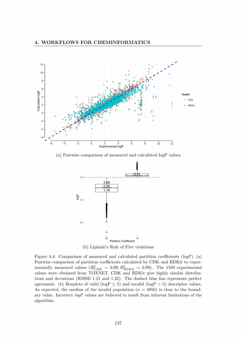
4. WORKFLOWS FOR CHEMINFORMATICS
−6
−4
−2
0
2
4
6
8
10
12
−6 −4 −2 0 2 4 6 8 10 12Experimental logP
Cal
cula
ted
logP Toolkit
CDK
RDKit
(a) Pairwise comparison of measured and calculated logP values
2.65
5.41
3.48
1.76
−5
0
5
Partition Coefficient
logP
≤5 >5
(b) Lipinski’s Rule of Five violations
Figure 4.4: Comparison of measured and calculated partition coefficients (logP). (a)Pairwise comparison of partition coefficients calculated by CDK and RDKit to exper-imentally measured values (R2
CDK = 0.99, R2RDKit = 0.99). The 1589 experimental
values were obtained from TOXNET. CDK and RDKit give highly similar distribu-tions and deviations (RMSD 1.21 and 1.22). The dashed blue line represents perfectagreement. (b) Boxplots of valid (logP ≤ 5) and invalid (logP > 5) descriptor values.As expected, the median of the invalid population (n = 4950) is close to the bound-ary value. Incorrect logP values are believed to result from inherent limitations of thealgorithm.
137

4. WORKFLOWS FOR CHEMINFORMATICS
Rule Violations
logP ≤ 5 4950
rotatable bonds ≤ 7 0 (24)
H−bond donors ≤ 5 0
H−bond acceptors ≤ 10 0
150 ≤ molecular weight ≤ 500 0
Table 4.1: Table of Lipinki’s Rule of Five violations for the ZINC dataset id:13 p0.0(134,322 structures) as calculated by KNIME-CDK. The 24 violations of the rotatablebonds rule result from the inclusion of amide bonds as rotatable bonds. This inclusionis not desirable due to the prohibitively high rotational energy barrier of amide C-Nbonds.
an approximate RMSD of 1.2, i.e. deviation by 1.2. The few large outliers –
beyond deviation – are believed to result from inherent limits of the algorithm.
Inspection of those outliers and cross-comparison with RDKit’s logP supports this
assumption: both toolkits estimate incorrect values for different subsets. Only
785 molecules have incorrect logP values in CDK and RDKit.
4.4.1 Round Tripping
Round tripping is a technique to evaluate information loss. In cheminformatics,
subtle differences in molecules such as inverted stereochemistry or addition/loss
of hydrogen, can significantly change molecular properties. Correct conversion of
one chemistry format into another is of paramount importance.
KNIME-CDK was tested using the same ChEBI set from the first round of eval-
uation (section 4.4). The SDfile was converted to CDK’s molecule representation
and then to CML. The CML was back-converted to CDK’s representation and fi-
nally to a SDfile. To accommodate for issues during SDfile generation, the SDfile
was read in again and converted to CML through CDK’s representation. The re-
sulting chemical representations were then compared to the original SDfile. This
process helped to find and eliminate format conversion errors.
138

4. WORKFLOWS FOR CHEMINFORMATICS
4.4.2 Test Workflows
KNIME-CDK uses workflow tests within the KNIME testing framework for qual-
ity assurance. More than a dozen workflows have been created to ensure correct
node behaviour in a variety of contexts, including different input formats, KNIME
table structures, and execution patterns or structures.
The tests reside on the KNIME testing server and are executed nightly. Different
test suits exist following the versioning system outlined in section 4.1. The con-
tinuous integration software Jenkins is used as integration tool checking builds
and test workflows.
4.4.3 Performance and Scalability
The plug-in performs well for tens of thousands of molecules. Whereas most
use-cases involve less than millions of molecules, KNIME-CDK has been tested
with up to 2,709,359 molecules taken from PubChem. Available memory and
the assigned number of threads are the two key limiting factors with regard to
execution speed.
An additional comparison with RDKit and Indigo [301] shows that the plug-in’s
bottleneck is molecule conversion (Figure 4.5a). Calculation or query performance
on converted molecules are comparable to RDKit and Indigo. Conversion to CML
combined with atom typing and aromaticity perception are the primary causes
for slow molecule conversion. Other toolkits use the one-line SMILES notation
that has high information density. However, SMILES notation does not allow
additional molecule information to be stored, a crucial drawback for CDK that
relies on atom types and perceived aromaticity. An additional speed penalty
comes from the used compression method to reduce disk requirements. Using
ChEBI, a seven fold reduction in CML file size is achieved on average during
serialization (14 kB to 2 kB) at the cost of seven seconds.
The bottleneck described above has been overcome in the nightly version of the
plug-in, which explores the advantages of SMILES: current evidence suggests that
139

4. WORKFLOWS FOR CHEMINFORMATICS
SMILES outperforms CML on the basis of speed and resource requirements. How-
ever, continuous re-perception of aromaticity and atom types – the advantages
of CML – increases the execution time. Increased in-memory execution time ap-
pears preferably over disk IO operations for IO-bound frameworks such as KNIME
(Figure 4.5b). Improvements in the CDK library in combination with improved
KNIME-CDK routines invert the picture seen in the comparison with the stable
builds. The nightly build outperforms RDKit and Indigo integrations.
4.5 Conclusion
KNIME-CDK is a community-driven plug-in with an active user base. The plug-
in is downloaded up to 600 times per month – download statistics are available
from the KNIME website, December 2013. It is actively maintained with efforts
focussing on extending the implemented functionality and improving overall us-
ability by automating standardization tasks. Over the last couple of years, the
underlying methods have been improved dramatically making the plug-in robust
and reliable. Together with improvements in the CDK library, a SMILES-backed
representation of molecular compounds appears to be the future. Molecule nor-
malization, e.g. tautomer selection and pKa calculations, remain dominant chal-
lenges to be addressed by the plug-in and the field of cheminformatics. To this
end, the tautomer generator will be extended and a set of nodes for normalization
will be introduced in the future.
4.6 Software Availability
KNIME-CDK and its JChemPaint, AMBIT, and Jmol dependencies have been
released under the GNU Lesser General Public License version 3. It depends on
the KNIME chemistry types, which are automatically added on installation.
140

4. WORKFLOWS FOR CHEMINFORMATICS
0.00.10.20.30.40.50.60.70.80.91.01.11.21.31.41.51.61.71.81.92.02.12.22.32.42.52.62.72.82.93.03.13.23.33.43.5
Conversion Substructure TotalFunction
Tim
e pe
r M
olec
ule
[ms]
Plugin
CDK
Indigo
RDKit
(a) KNIME execution time comparison: v 2.9
0.000.050.100.150.200.250.300.350.400.450.500.550.600.650.700.750.800.850.900.951.001.051.101.151.20
Conversion Substructure TotalFunction
Tim
e pe
r M
olec
ule
[ms]
Plugin
CDK
Indigo
RDKit
(b) KNIME execution time comparison: nightly build
Figure 4.5: Comparison of average execution times per molecule by cheminformaticsplug-in. The total time measured equals the sum of the molecule conversion and phenylsubstructure search. (a) CDK version 1.4.4, Indigo version 1.1.13, and RDKit version2.2.0 were used for the comparison. KNIME-CDK is five fold slower than the otherplug-ins during conversion and as fast as the other plug-ins during substructure search.Molecule conversion is the bottleneck of KNIME-CDK. (b) Comparison of nightly builds(CDK version 1.5.1, Indigo version 1.1.13, and RDKit version 2.4.0): KNIME-CDK ison average four and a half fold faster than the other plug-ins.
141

4. WORKFLOWS FOR CHEMINFORMATICS
4.6.1 Update Site
The project is part of KNIME’s Community Contributions and hosted on their
servers. It can be installed via the official Community Contributions update sites.
The entry pages are listed below:
• KNIME-CDK: https://bitbucket.org/sbeisken/cdkknime
• KNIME-CDK Support: http://tech.knime.org/community/cdk
• KNIME Update Site:
http://tech.knime.org/update/community-contributions/<version>
4.6.2 Extensions
KNIME-CDK is a community-driven project that develops by improvements on
its core library CDK and feature requests in the KNIME-CDK forum. Node devel-
opment follows the KNIME node development guidelines. Contributions should
be directed to the central KNIME-CDK subversion repository on the KNIME
servers.
• KNIME-CDK Forum: http://tech.knime.org/forum/cdk
4.6.3 Example Workflows
Example workflows illustrating the basics of KNIME-CDK and more advanced
applications, such as R integration and data mining, have been deposited on
MyExperiment [221] under the keyword ‘KNIME-CDK’.
Use cases of workflows using KNIME-CDK include the management and analysis
of chemical libraries through molecular descriptors, conformer analysis via RMSD,
and NMR spectra prediction.
The work has been published in BMC Bioinformatics: Beisken et al.: KNIME-
CDK: Workflow-driven Cheminformatics. BMC Bioinformatics 2013, 14:257.
doi:10.1186/1471-2105-14-257
142

CHAPTER 5
Summary and Discussion
Metabolomics is based on analytical technologies that capture data about low
molecular weight compounds. Information contained in the data can be distilled
through careful data processing and analysis. The high chemical diversity, concen-
tration differences, and dynamics of the metabolome complicate this task.
Detailed electronic logbooks have become fashionable in experimental laborato-
ries. The need to additionally capture the complete digital analysis process as well
is becoming a dominant theme in metabolomics. Transparency and reproducibil-
ity are key elements to guarantee scalable research within the science community.
The ability to share and reuse not only data but also workflows or pipelines is
important. Open, ‘copyleft’, licenses form the foundation for data exchange and
boundary-free informatics in metabolomics.
Tandem mass spectrometry systems coupled to liquid chromatography (LC-MSn)
capture detailed metabolomics snapshots of biological samples under controlled
conditions. The resulting data sets are convoluted, noisy, and their fine struc-
ture is dependent on a plethora of parameters and external factors. Full control
over the applied data processing steps is required. Modularity, i.e. the effective
addition or removal of individual functions, extendibility, and visual feedback
are desirable criteria for any processing tool applied to the task of LC-MSn data
exploration and analysis.
143

5. SUMMARY AND DISCUSSION
Informatics for LC-MSn Analysis: We created MassCascade, a framework to
rapidly analyse and visualise LC-MSn data. The framework covers all processing
steps from data input to the final generation of the feature matrix. It features
a plug-in for the popular workflow platform KNIME, which integrates comple-
mentary statistical, bio- and cheminformatics functionality that can be used in
combination with MassCascade-KNIME. The plug-in offers a structured approach
to data processing in metabolomics that is accessible to bioinformaticians and ex-
perimental scientists alike.
Developed in collaboration with the Syngenta AG, MassCascade does not aim
to reproduce existing processing tools for LC-MSn data but offers a different
approach following the paradigm of visual programming. Its focus on feature fil-
tering with multiple ways to remove irrelevant features and its rapid applicability
to repetitive processing steps, make it useful for calibration exercises or spectral
fingerprinting.
Knowledge-based Compound Identification: We added an identification and scor-
ing framework to MassCascade that also integrates seamlessly into the workflow
plug-in. The framework enables the generation of reference or spectra libraries
for multiple MS level from reference data. It automatically scores and ranks re-
trieved feature annotations from these reference libraries based on information
aggregated during processing, e.g. from isotopic envelopes and from the putative
structures themselves. The ranked lists of annotations for every feature of interest
simplify metabolite identification.
The metabolites extracted from the study on metabolite ripening demonstrates
the use of the methodology and highlights the importance of fragment infor-
mation. The combination of uni- and multivariate statistics with the ability to
rapidly change back to the processing side and fine-tune the workflow using purely
open tools, guarantees flexibility and transparency that dramatically facilitates
data sharing, e.g. study deposition in the MetaboLights repository or submission
of a Nature Scientific Data manuscript.
144

5. SUMMARY AND DISCUSSION
Workflows for Cheminformatics: LC-MSn post-processing relies on cheminfor-
matics for the convenience of handling and visualizing putative metabolites. From
the input of small molecule collections, e.g. from plain files, to the selection of
molecule subsets based on molecular properties or the generation of molecular
formulas from exact molecular masses, cheminformatics has many applications
in the context of metabolomics mass spectrometry. We contributed a cheminfor-
matics plug-in based on the Chemistry Development Kit (CDK) to the workflow
platform that also hosts MassCascade to provide such functionality and facilitate
metabolite identification efforts.
The use cases of the user base exceed far beyond applications in LC-MSn. The
tool is primarily used as solid cheminformatics toolkit. With a broad user base, it
is primarily community driven. Together with our tools and other external plug-
ins, it forms a powerful, consolidated set for applications in the life sciences.
Future work involves fine-tuning and further validation of the implemented meth-
ods. Differences in resolution of mass spectrometers is only one factor that can
have a dramatic impact on data analysis. To provide starting points for data anal-
ysis for different instruments, we aim to establish workflows for these instruments
that may serve as templates.
To improve the metabolite identification pipeline, we will adopt methods to gen-
erate fragmentation spectra (in silico) that also give predicted signal abundances.
As discussed, this is most likely to increase the power of the scoring framework
for annotations from highly similar molecular species.
The KNIME-CDK plug-in evolves continuously together with the CDK core li-
brary. To increase its use, molecule normalisation has been singled out as primary
area for future work. A collection of nodes will be implemented to simplify the
management of sets of molecules.
The high throughput and multivariate data generating nature of metabolomics
experiments requires substantial informatics. It the responsibility of the informat-
ics toolkits to simplify data analysis as far as possible while recording everything
within the processing pipeline. The tools developed and tested here have been
designed to follow these principles. Whereas spectral fingerprinting of biological
145

5. SUMMARY AND DISCUSSION
samples is challenging, the major bottleneck in metabolomics is metabolite identi-
fication. The aggregation and rationalisation of information from mass spectrom-
etry experiments in a structured manner enables the generation of ranked lists of
identifications that also reflect confidence. Identifications with certainty are rare
however and require additional evidence only attainable through laboratory work.
Tools that facilitate the complete process and show the complexity of processing
and ambiguity in identification are small steps in the right direction.
Metabolomics is at a junction. While experimental systems are improving, re-
producible metabolite identification is still challenging in metabolomics studies.
This is particularly true for unknown metabolites that have not been recorded
in previous studies. Whereas some instrumental systems can confidently detect
many small molecules from the core metabolism, going beyond that into truly
untargeted metabolomics will depend on the existence of high quality, large-scale
reference databases and informed information aggregation.
146

Appendix
Univariate Statistics for Feature Analysis
The following figures describe the 13 unique features investigated in chapter 3.5.
Univariate statistics for the seven features not discussed in chapter 3.5.3 are shown
after. Pairwise Person’s correlation matrices were built for each genotype with
asymptotic p-values encoded in a three star asterisk representation.
−10
−5
0
5
10
15
20
0 15 30 45 60 75 90 105Sample Number
Rel
ativ
e A
bund
ance
m/z: 343.296 AC++ CNR NOR RIN
−10
−5
0
5
10
15
20
AC++ CNR NOR RINGenotype
Rel
ativ
e A
bund
ance
0.00
0.25
0.50
0.75
1.00
0.00 0.25 0.50 0.75 1.00False positive rate
True
pos
itive
rat
e
Figure 1: Univariate statistics for feature 343.296. The scatterplot shows feature abun-dances grouped by genotype and sorted by harvest date in ascending order with appliedlocally weighted smoothing. The boxplots display the median (middle line) and lower(25%) and upper (75%) percentiles of the abundances. The ROC curves indicate thebinary classification power of the mutant genotypes versus the wild type AC++.
147

Appendix
−1.000
−0.375
0.250
0.875
1.500
2.125
2.750
3.375
4.000
0 15 30 45 60 75 90 105Sample Number
Rel
ativ
e A
bund
ance
m/z: 140.006 AC++ CNR NOR RIN
−1.000
−0.375
0.250
0.875
1.500
2.125
2.750
3.375
4.000
AC++ CNR NOR RINGenotype
Rel
ativ
e A
bund
ance
0.00
0.25
0.50
0.75
1.00
0.00 0.25 0.50 0.75 1.00False positive rate
True
pos
itive
rat
e(a) Univariate statistics for feature 140.006
−2
−1
0
1
2
3
4
0 15 30 45 60 75 90 105Sample Number
Rel
ativ
e A
bund
ance
m/z: 211.169 AC++ CNR NOR RIN
−2
−1
0
1
2
3
4
AC++ CNR NOR RINGenotype
Rel
ativ
e A
bund
ance
0.00
0.25
0.50
0.75
1.00
0.00 0.25 0.50 0.75 1.00False positive rate
True
pos
itive
rat
e
(b) Univariate statistics for feature 211.169
Figure 2: Univariate statistics for features 140.006 (a) and 211.169 (b). The scatterplotshows feature abundances grouped by genotype and sorted by harvest date in ascend-ing order with applied locally weighted smoothing. The boxplots display the median(middle line) and lower (25%) and upper (75%) percentiles of the abundances. TheROC curves indicate the binary classification power of the mutant genotypes versusthe wild type AC++.
148

Appendix
−7
−5
−3
−1
1
3
5
7
9
0 15 30 45 60 75 90 105Sample Number
Rel
ativ
e A
bund
ance
m/z: 232.114 AC++ CNR NOR RIN
−7
−5
−3
−1
1
3
5
7
9
AC++ CNR NOR RINGenotype
Rel
ativ
e A
bund
ance
0.00
0.25
0.50
0.75
1.00
0.00 0.25 0.50 0.75 1.00False positive rate
True
pos
itive
rat
e
(a) Univariate statistics for feature 232.114
−20.00
−13.75
−7.50
−1.25
5.00
11.25
17.50
23.75
30.00
0 15 30 45 60 75 90 105Sample Number
Rel
ativ
e A
bund
ance
m/z: 299.183 AC++ CNR NOR RIN
−20.00
−13.75
−7.50
−1.25
5.00
11.25
17.50
23.75
30.00
AC++ CNR NOR RINGenotype
Rel
ativ
e A
bund
ance
0.00
0.25
0.50
0.75
1.00
0.00 0.25 0.50 0.75 1.00False positive rate
True
pos
itive
rat
e
(b) Univariate statistics for feature 299.183
Figure 3: Univariate statistics for features 232.114 (a) and 299.183 (b). The scatterplotshows feature abundances grouped by genotype and sorted by harvest date in ascend-ing order with applied locally weighted smoothing. The boxplots display the median(middle line) and lower (25%) and upper (75%) percentiles of the abundances. TheROC curves indicate the binary classification power of the mutant genotypes versusthe wild type AC++.
149

Appendix
−3.00
−1.75
−0.50
0.75
2.00
3.25
4.50
5.75
7.00
0 15 30 45 60 75 90 105Sample Number
Rel
ativ
e A
bund
ance
m/z: 330.009 AC++ CNR NOR RIN
−3.00
−1.75
−0.50
0.75
2.00
3.25
4.50
5.75
7.00
AC++ CNR NOR RINGenotype
Rel
ativ
e A
bund
ance
0.00
0.25
0.50
0.75
1.00
0.00 0.25 0.50 0.75 1.00False positive rate
True
pos
itive
rat
e(a) Univariate statistics for feature 330.009
−10
−5
0
5
10
15
20
0 15 30 45 60 75 90 105Sample Number
Rel
ativ
e A
bund
ance
m/z: 125.112 AC++ CNR NOR RIN
−10
−5
0
5
10
15
20
AC++ CNR NOR RINGenotype
Rel
ativ
e A
bund
ance
0.00
0.25
0.50
0.75
1.00
0.00 0.25 0.50 0.75 1.00False positive rate
True
pos
itive
rat
e
(b) Univariate statistics for feature 125.112
Figure 4: Univariate statistics for features 330.009 (a) and 125.112 (b). The scatterplotshows feature abundances grouped by genotype and sorted by harvest date in ascend-ing order with applied locally weighted smoothing. The boxplots display the median(middle line) and lower (25%) and upper (75%) percentiles of the abundances. TheROC curves indicate the binary classification power of the mutant genotypes versusthe wild type AC++.
150

Appendix
−0.25 0.14 −0.77 −0.30 −0.59 −0.33 −0.45 −0.22 −0.07 −0.60 −0.38 0.01
−0.60 −0.15 0.11 0.06 0.16 0.51 0.52 0.60 0.58 0.35 0.43
−0.03 −0.28 −0.36 −0.41 −0.47 −0.45 −0.78 −0.39 −0.35 −0.55
0.18 0.70 0.19 0.27 −0.05 −0.35 0.36 0.34 0.01
0.30 0.42 0.16 0.25 0.23 0.14 0.05 −0.01
0.31 0.41 0.20 −0.07 0.37 0.34 0.28
0.44 0.34 0.31 0.34 0.52 −0.01
0.79 0.23 0.54 0.78 0.40
0.34 0.41 0.50 0.32
0.27 0.09 0.26
0.42 0.34
0.15
*** *** * ***
*** *** *** *** *** *
* * * *** * ***
***
*
*
* ***
*** *** *** *
* *
*
118.09
125.11
130.05
133.06
140.01
176.1
197.1
211.17
232.11
299.18
327.12
330.01
343.3
−0.5
0.0
0.5
1.0R^2
(a) Pairwise Pearson’s correlation matrix for WT AC++
0.11 0.38 −0.74 0.23 0.45 −0.08 0.03 −0.07 −0.35 0.15 0.02 −0.07
−0.17 −0.26 0.15 −0.35 0.66 0.51 0.45 −0.11 0.57 0.56 0.10
−0.37 0.03 0.67 −0.15 −0.27 −0.35 −0.69 −0.38 −0.37 −0.27
−0.12 −0.42 0.01 0.07 0.16 0.01 −0.08 −0.07 0.10
0.23 0.08 0.08 0.18 −0.27 0.10 0.21 0.27
−0.39 −0.56 −0.56 −0.40 −0.49 −0.44 −0.12
0.66 0.59 −0.25 0.52 0.46 0.19
0.89 −0.19 0.87 0.72 0.16
−0.17 0.75 0.76 0.35
−0.04 −0.06 −0.15
0.71 0.20
0.51
*** *
*** *** * *** ***
*** ***
*
*** *** * * *
*** *** *** *
*** *** ***
*** ***
***
***
118.09
125.11
130.05
133.06
140.01
176.1
197.1
211.17
232.11
299.18
327.12
330.01
343.3
−0.5
0.0
0.5
1.0R^2
(b) Pairwise Pearson’s correlation matrix for mutant CNR
Figure 5: Pearson’s pairwise correlation matrix for wild type AC++ (a) and mutantCNR (b). The asymptotic p-values are encoded using asterisks: p ≤ 0.01 = ∗ ∗ ∗,0.01 < p ≤ 0.05 = ∗. The correlation coefficient ranges from low, R2 ≤ −0.5 (darkblue), to high, R2 ≥ 0.5 (bright red).
151

Appendix
0.23 0.19 −0.53 −0.18 −0.44 −0.23 0.03 0.29 −0.42 −0.40 −0.15 0.10
−0.16 0.04 0.01 0.08 −0.22 0.04 −0.09 −0.33 0.25 −0.13 0.16
−0.55 0.09 −0.14 −0.10 0.13 0.27 −0.30 −0.45 0.14 −0.23
−0.01 0.15 0.05 0.01 −0.31 −0.23 0.69 0.16 0.05
0.27 0.23 0.19 −0.02 −0.05 −0.01 0.13 0.28
0.12 0.01 −0.21 0.01 0.01 0.26 0.29
0.14 −0.08 0.14 0.01 −0.00 −0.01
0.64 −0.26 −0.02 0.45 0.03
−0.17 −0.16 0.43 0.05
−0.12 −0.31 −0.22
0.24 0.18
0.30
*** * * *
*** *
***
*** *
*
118.09
125.11
130.05
133.06
140.01
176.1
197.1
211.17
232.11
299.18
327.12
330.01
343.3
−0.5
0.0
0.5
1.0R^2
(a) Pearson’s pairwise correlation matrix for mutant NOR
0.13 0.11 −0.73 −0.26 −0.49 0.20 −0.10 −0.06 −0.25 −0.38 −0.09 0.16
−0.25 −0.37 −0.20 0.26 0.31 0.55 0.29 0.03 0.15 0.30 0.22
0.09 −0.20 0.06 −0.23 −0.40 −0.32 −0.75 −0.54 −0.10 −0.25
0.11 0.37 −0.39 −0.18 −0.18 −0.24 0.28 −0.24 −0.33
−0.02 −0.22 0.30 0.27 0.26 0.20 0.37 0.19
−0.07 0.17 0.02 −0.18 0.29 0.10 −0.17
0.02 0.09 0.19 0.13 −0.05 −0.20
0.85 0.16 0.45 0.75 0.65
0.13 0.50 0.71 0.69
0.21 0.08 0.11
0.35 0.39
0.66
*** *
***
* *** ***
*** * *** ***
*** *** ***
*
***
118.09
125.11
130.05
133.06
140.01
176.1
197.1
211.17
232.11
299.18
327.12
330.01
343.3
−0.5
0.0
0.5
1.0R^2
(b) Pearson’s pairwise correlation matrix for mutant RIN
Figure 6: Pearson’s pairwise correlation matrix for mutants NOR (a) and RIN (b). Theasymptotic p-values are encoded using asterisks: p ≤ 0.01 = ∗ ∗ ∗, 0.01 < p ≤ 0.05 = ∗.The correlation coefficient ranges from low, R2 ≤ −0.5 (dark blue), to high, R2 ≥ 0.5(bright red).
152

Appendix
Identification
Rankings
Name Depiction Score
Frag. Isotope None
L-citrulline* n/a 260 160
Table 1: Metabolite annotation for m/z 176.103 with cumulative scores for no, isotope,and fragment filtering. Missingness and element filters were always included. Thecalculated score does not allow for selective ranking. All structures are highly similar.*Matching retention time information in the in-house library at 95 seconds.
Name Depiction Score
Frag. Isotope None
trans-4-hydroxystilbene†
369 251 160
cis-stilbene oxide 369 251 160
MS2 spectrum
Table 2: Metabolite annotations for m/z 197.096 with cumulative scores for no, isotope,and fragment filtering. Missingness and element filters were always included. Thecalculated score does not allow for selective ranking. All structures are highly similar.†The extracted MS2 spectrum shown at the bottom of the table is dominated by a peakat 105.033 (putative structure shown).
153

Appendix
Name Depiction Score
Frag. Isotope None
humilixanthin n/a 410 160
Table 3: Metabolite annotations for m/z 327.117 with cumulative scores for no, isotope,and fragment filtering. Missingness and element filters were included by default.
Molecular Formula Generation
Table 4 lists the 13 features that were singled out for identification. Molecular
formulas were calculated for the charge corrected features within a 0.05 amu mass
tolerance (Table 5). Structures were generated via Molgen using the command
below. The ‘badlist’ is contained in the program and contains forbidden structures
to be discarded when encountered during the deterministic structure generation
process.
mgen.exe <file_in> -cycles 0-2 -ringsize 0-10
-o <file_out> -stop 50 -badlist badlist.sdf
Feature m/z Feature m/z
118.086 197.096
125.112 211.169
130.050 232.114
133.061 299.183
140.011 327.118
176.103 330.009
343.296
Table 4: Extracted features for identification.
Molecular Weight Molecular Formula Molecular Weight Molecular Formula
117.029 CH3N5O2 210.141 CH14N12O
117.033 C6H3N3 210.153 H14N14
117.04 H3N7O 231.056 CH9N7O7
117.043 C4H7NO3 231.058 C2H5N11O3
154

Appendix
Molecular Weight Molecular Formula Molecular Weight Molecular Formula
117.054 C3H7N3O2 231.059 C5H13NO9
117.058 C8H7N 231.06 C6H9N5O5
117.065 C2H7N5O 231.062 C7H5N9O
117.076 CH7N7 231.064 C11H9N3O3
117.079 C5H11NO2 231.068 H9N9O6
117.09 C4H11N3O 231.069 CH5N13O2
117.101 C3H11N5 231.07 C4H13N3O8
117.115 C6H15NO 231.072 C5H9N7O4
117.127 C5H15N3 231.073 C6H5N11
124.06 CH8N4O3 231.074 C9H13NO6
124.064 C6H8N2O 231.076 C10H9N5O2
124.071 H8N6O2 231.08 C15H9N3
124.075 C5H8N4 231.08 H5N15O
124.089 C8H12O 231.081 C3H13N5O7
124.1 C7H12N2 231.083 C4H9N9O3
129.006 C4H3NO4 231.086 C8H13N3O5
129.017 C3H3N3O3 231.087 C9H9N7O
129.021 C8H3NO 231.09 C13H13NO3
129.029 C2H3N5O2 231.093 C2H13N7O6
129.033 C7H3N3 231.094 C3H9N11O2
129.04 CH3N7O 231.097 C7H13N5O4
129.043 C5H7NO3 231.098 C8H9N9
129.051 H3N9 231.101 C12H13N3O2
129.054 C4H7N3O2 231.104 CH13N9O5
129.058 C9H7N 231.105 C2H9N13O
129.065 C3H7N5O 231.108 C6H13N7O3
129.076 C2H7N7 231.112 C11H13N5O
129.079 C6H11NO2 231.115 H13N11O4
129.09 C5H11N3O 231.117 CH9N15
132.003 N6O3 231.119 C5H13N9O2
132.006 C4H4O5 231.123 C10H13N7
132.007 C5N4O 231.13 C4H13N11O
132.017 C3H4N2O4 231.142 C3H13N13
132.018 C4N6 298.129 C13H14N8O
132.021 C8H4O2 298.132 C2H14N14O4
132.028 C2H4N4O3 298.136 C7H14N12O2
132.032 C7H4N2O 298.14 C12H14N10
132.04 CH4N6O2 298.148 C6H14N14O
132.042 C5H8O4 326.061 C10H10N6O7
132.044 C6H4N4 326.062 C11H6N10O3
155

Appendix
Molecular Weight Molecular Formula Molecular Weight Molecular Formula
132.051 H4N8O 326.064 C14H14O9
132.053 C4H8N2O3 326.065 C15H10N4O5
132.058 C9H8O 326.067 C3H14N6O12
132.065 C3H8N4O2 326.068 C4H10N10O8
132.069 C8H8N2 326.07 C5H6N14O4
132.076 C2H8N6O 326.071 C8H14N4O10
132.079 C6H12O3 326.072 C9H10N8O6
132.087 CH8N8 326.074 C10H6N12O2
132.09 C5H12N2O2 326.075 C13H14N2O8
132.094 C10H12 326.076 C14H10N6O4
132.101 C4H12N4O 326.078 C15H6N10
138.975 CHNO7 326.078 C2H14N8O11
138.987 HN3O6 326.08 C3H10N12O7
138.991 C5HNO4 326.082 C7H14N6O9
139.002 C4HN3O3 326.084 C8H10N10O5
139.006 C9HNO 326.085 C9H6N14O
139.012 C2H5NO6 326.086 C12H14N4O7
139.013 C3HN5O2 326.088 C13H10N8O3
139.017 C8HN3 326.089 CH14N10O10
139.023 CH5N3O5 326.091 C2H10N14O6
139.024 C2HN7O 326.093 C6H14N8O8
139.027 C6H5NO3 326.095 C7H10N12O4
139.034 H5N5O4 326.097 C11H14N6O6
139.035 CHN9 326.099 C12H10N10O2
139.038 C5H5N3O2 326.101 H14N12O9
139.042 C10H5N 326.105 C5H14N10O7
139.048 C3H9NO5 326.106 C6H10N14O3
139.049 C4H5N5O 326.109 C10H14N8O5
175.045 C2H5N7O3 326.11 C11H10N12O
175.048 C6H9NO5 326.113 C15H14N6O3
175.049 C7H5N5O 326.116 C4H14N12O6
175.057 CH5N9O2 326.12 C9H14N10O4
175.059 C5H9N3O4 326.121 C10H10N14
175.061 C6H5N7 326.124 C14H14N8O2
175.063 C10H9NO2 326.127 C3H14N14O5
175.068 H5N11O 326.131 C8H14N12O3
175.071 C4H9N5O3 326.135 C13H14N10O
175.075 C9H9N3O 326.142 C7H14N14O2
175.082 C3H9N7O2 326.146 C12H14N12
175.084 C7H13NO4 328.962 C5H3N3O14
156

Appendix
Molecular Weight Molecular Formula Molecular Weight Molecular Formula
175.086 C8H9N5 328.966 C10H3NO12
175.093 C2H9N9O 328.973 C4H3N5O13
175.096 C6H13N3O3 328.977 C9H3N3O11
175.1 C11H13NO 328.981 C14H3NO9
175.104 CH9N11 328.984 C3H3N7O12
175.107 C5H13N5O2 328.987 C7H7NO14
175.111 C10H13N3 328.988 C8H3N5O10
175.118 C4H13N7O 328.992 C13H3N3O8
175.129 C3H13N9 328.994 CH7N5O15
196.039 C10H4N4O 328.995 C2H3N9O11
196.043 N14 328.998 C6H7N3O13
196.044 C3H8N4O6 328.999 C7H3N7O9
196.046 C4H4N8O2 329.002 C11H7NO11
196.048 C8H8N2O4 329.003 C12H3N5O7
196.05 C9H4N6 329.005 H7N7O14
196.052 C13H8O2 329.006 CH3N11O10
196.056 C2H8N6O5 329.009 C5H7N5O12
196.057 C3H4N10O 329.01 C6H3N9O8
196.058 C6H12O7 329.013 C10H7N3O10
196.06 C7H8N4O3 329.014 C11H3N7O6
196.064 C12H8N2O 329.017 C15H7NO8
196.067 CH8N8O4 329.018 H3N13O9
196.068 C2H4N12 329.019 C3H11N3O15
196.07 C5H12N2O6 329.02 C4H7N7O11
196.071 C6H8N6O2 329.022 C5H3N11O7
196.074 C10H12O4 329.023 C8H11NO13
196.075 C11H8N4 329.024 C9H7N5O9
196.078 H8N10O3 329.026 C10H3N9O5
196.081 C4H12N4O5 329.028 C14H7N3O7
196.082 C5H8N8O 329.03 C15H3N7O3
196.085 C9H12N2O3 329.03 C2H11N5O14
196.089 C14H12O 329.032 C3H7N9O10
196.092 C3H12N6O4 329.033 C4H3N13O6
196.093 C4H8N10 329.034 C7H11N3O12
196.096 C8H12N4O2 329.036 C8H7N7O8
196.1 C13H12N2 329.037 C9H3N11O4
196.103 C2H12N8O3 329.038 C12H11NO10
196.107 C7H12N6O 329.04 C13H7N5O6
196.114 CH12N10O2 329.041 C14H3N9O2
196.118 C6H12N8 329.041 CH11N7O13
157

Appendix
Molecular Weight Molecular Formula Molecular Weight Molecular Formula
196.126 H12N12O 329.043 C2H7N11O9
210.112 C9H14N4O2 329.044 C3H3N15O5
210.116 C14H14N2 329.046 C6H11N5O11
210.119 C3H14N8O3 329.047 C7H7N9O7
210.123 C8H14N6O 329.048 C8H3N13O3
210.13 C2H14N10O2 329.05 C11H11N3O9
210.134 C7H14N8
Table 5: Molecular formulas calculated from the extracted features within a 0.05 amumass window. Incorrect formulas were filtered out using the seven golden rules de-scribed by Kind et al. [240].
158

Appendix
Unsupported Structures in KNIME-CDK
(a) Cob(II)alamin (CHEBI:16304) (b) Nitrogen dioxide (CHEBI:33101)
(c) Chlorophyll b (CHEBI:2788) (d) Arsanyl (CHEBI:33105)
(e) 14-C-Glycylpeptide (CHEBI:65304) (f) Vanadium (CHEBI:27698)
Figure 7: Examples of chemical classes that lack support in KNIME-CDK. (a)Coordination entities (CHEBI:16304), (b, d) some radical species (CHEBI:33101,CHEBI:33105), (c) complexed porphyrins (CHEBI:27888), (e) repeated structures(CHEBI:65304), and (f) exotic atoms (CHEBI:27698).
159

Appendix
LC-MS Interferents
List of potential interference ions in positive ion mode LC-ESI-MS up to 1000
Da. The list was adapted from Keller et al. [110]. The ion mass, ion type, formula,
and chemical species is provided.
Ion Mass Ion Type Formula or Subunit Species
33.03349 [M+H]+ CH3OH Methanol
42.03383 [M+H]+ CH3CN ACN
59.06037 [M+NH4]+ CH3CN ACN
63.04406 [A1B+H]+ [C2H4O]nH2O PEG
64.01577 [M+Na]+ CH3CN ACN
65.05971 [M2+H]+ CH3OH Methanol
74.06004 [M+H]+ C3H7NO Dimethyl formamide
74.06004 [A1B1+H]+ (CH3CN)n(CH3OH)m Acetonitrile/Methanol
77.05971 [A1B+H]+ [C3H6O]nH2O PPG
79.02121 [M+H]+ C2H6OS DMSO
83.06037 [M2+H]+ CH3CN Acetonitrile
85.02600 [A1B+Na]+ [C2H4O]nH2O PEG
85.05887 [M+H]+ C2D6OS d6-DMSO
88.03931 [A1B1+H]+ (CH3CN)n(HCOOH)m Acetonitrile/Formic Acid
96.04198 [A1B1+Na]+ (CH3CN)n(CH3OH)m Acetonitrile/Methanol
99.04165 [A1B+Na]+ [C3H6O]nH2O PPG
100.07569 [M+H]+ C5H10NO NMP
100.99994 [A1B+K]+ [C2H4O]nH2O PEG
101.00316 [M+Na]+ C2H6OS DMSO
101.08084 [A2B2+H]+ [MeOH]n[H2O]m Methanol/Water
102.05496 [A1B1+H]+ (CH3CN)n(CH3COOH)m Acetonitrile/Acetic Acid
102.12773 [M+H]+ C6H15N TEA
103.95560 [M+H]+ C2H3N ACN
104.99229 [M+Na]+ C2H3O2Na Sodium acetate
105.04232 [M2+Na]+ C2H3N ACN
105.95379 [M+65Cu]+ C2H3N ACN
107.07027 [A2B+H]+ [C2H4O]nH2O PEG
115.01559 [A1B+K]+ [C3H6O]nH2O PPG
115.08659 [A1B1+H]+ (CH3CN)n(C3H7NO)m Acetonitrile/Dimethylformamide
120.04776 [M+CH3CN+H]+ C2H6OS DMSO
122.08117 [M+H]+ C4H11NO3 TRIS
123.06278 [A2B2+Na]+ [MeOH]n[H2O]m Methanol/Water
123.09167 [M+H]+ C7H10N2 DMAP
124.03690 [A1B1+Na]+ (CH3CN)n(CH3COOH)m Acetonitrile/Acetic Acid
129.05222 [A2B+Na]+ [C2H4O]nH2O PEG
130.15903 [M+H]+ C8H19N DIPEA132.90490 M+ Cs Cs-133
133.10705 [A3B2+H]+ [MeOH]n[H2O]m Methanol/Water
135.10157 [A2B+H]+ [C3H6O]nH2O PPG
137.07431 [M+CH3CN+NH4]+ C2H6OS DMSO
142.02971 [M+CH3CN+Na]+ C2H6OS DMSO
144.17468 [M+H]+ C9H21N TPA
144.98215 [M2+63Cu]+ CH3CN ACN
145.02615 [A2B+K]+ [C2H4O]nH2O PEG
146.06887 [M3+Na]+ CH3CN ACN
146.98034 [M2+65Cu]+ CH3CN ACN
160

Appendix
Ion Mass Ion Type Formula or Subunit Species
147.11280 [A2B2+H]+ (CH3CN)n(CH3OH)m Acetonitrile/Methanol
149.02332 [f+H]+ C8H4O3 Pthalic Anhydride
150.12773 [M+H]+ C10H15N Phenyldiethylamine
151.09649 [A3B+H]+ [C2H4O]nH2O PEG
153.13862 [M+H]+ C9H16N2 DBU
155.08900 [A3B2+Na]+ [MeOH]n[H2O]m Methanol/Water
157.03515 [M2+H]+ C2H6OS DMSO
157.08352 [A2B+Na]+ [C3H6O]nH2O PPG
158.96403 [M+Na]+ C2F3O2Na NaTFA
163.03897 [M− CH3OH+H]+ C10H10O4 Dimethyl phthalate
163.13287 [M+H]+ C8H18O3 DGBE
169.09475 [A2B2+Na]+ (CH3CN)n(CH3OH)m Acetonitrile/Methanol
169.11046 [M2+H]+ C2D6OS d6-DMSO
171.00527 [f+Na]+ C8H4O3 Phthalic anhydride
172.03931 [M−H2O+H]+ C10H7NO3 4-HCCA
173.05745 [A2B+K]+ [C3H6O]nH2O PPG
173.07843 [A3B+Na]+ [C2H4O]nH2O PEG
179.01709 [M2+Na]+ C2H6OS DMSO
181.12231 [M+H]+ C11H16O2 BHA
183.08044 [M+H]+ C13H10O DPK
183.14383 [A4B3+H]+ [MeOH]n[H2O]m Methanol/Water
185.11482 [M+Na]+ C8H18O3 GE
186.22163 [M+H]+ C12H27N TBA
189.05237 [A3B+K]+ [C2H4O]nH2O PEG
190.04987 [M+H]+ C10H7NO3 4-HCCA
193.14344 [A3B+H]+ [C3H6O]nH2O PPG
195.06519 [M+H]+ C10H10O4 Dimethyl phthalate
195.12270 [A4B+H]+ [C2H4O]nH2O PEG
203.10425 [M+Na]+ C11H16O2 BHA
205.12578 [A4B3+Na]+ [MeOH]n[H2O]m Methanol/Water
212.03181 [M+Na]+ C10H7NO3 4-HCCA
214.08963 [M+H]+ C10H15NO2S n-BBS
215.12538 [A3B+Na]+ [C3H6O]nH2O PPG
217.10465 [A4B+Na]+ [C2H4O]nH2O PEG
221.18999 [M+H]+ C15H24O BTH
225.19614 [M+H]+ C13H24N2O DCU
228.00575 [M+K]+ C10H7NO3 4-HCCA
231.09932 [A3B+K]+ [C3H6O]nH2O PPG
231.11618 [M+NH4]+ C10H15NO2S n-BBS
233.07858 [A4B+K]+ [C2H4O]nH2O PEG
236.07157 [M+Na]+ C10H15NO2S n-BBS
239.14892 [A5B+H]+ [C2H4O]nH2O PEG
239.22485 [(M.H35Cl)2 − Cl]+ C6H15N TEA.HCl
241.22190 [(M.H37Cl)2 − Cl]+ C6H15N TEA.HCl242.28423 M+ C16H36N TBA243.11683 M+ C19H15 Trityl cation
243.17194 [M+Na]+ C15H24O BTH
251.18530 [A4B+H]+ [C3H6O]nH2O PPG
251.20056 [AB1+H]+ [C14H22O][C2H4O]n Triton
257.03103 [M3+Na]+ C2H6OS DMSO
261.13086 [A5B+Na]+ [C2H4O]nH2O PEG
265.21621 [AB1+H]+ [C15H24O][C2H4O]n Triton
267.17197 [M+H]+ C12H27O4P TBP273.12739 M+ C20H17O MMT
273.16725 [A4B+Na]+ [C3H6O]nH2O PPG
273.18250 [AB1+Na]+ [C14H22O][C2H4O]n Triton
161

Appendix
Ion Mass Ion Type Formula or Subunit Species
277.10480 [A5B+K]+ [C2H4O]nH2O PEG
279.09333 [M+H]+ C18H15OP TPO
279.15909 [M+H]+ C16H22O4 Dibutylphthalate
279.22945 [AB1+Na]+ [C14H28O][C2H4O]n Triton, reduced
282.27914 [M+H]+ C18H35NO Oleamide
283.17513 [A6B+H]+ [C2H4O]nH2O PEG
284.29479 [M+H]+ C18H37NO Stearamide
287.19815 [AB1+Na]+ [C15H24O][C2H4O]n Triton
288.25332 [M+H]+ C16H33NO3 n,n-DDA
289.14118 [A4B+K]+ [C3H6O]nH2O PPG
293.24510 [AB1+Na]+ [C15H30O][C2H4O]n Triton, reduced
295.22677 [AB2+H]+ [C14H22O][C2H4O]n Triton
301.14103 [M+Na]+ C16H22O4 Dibutylphthalate
304.26108 [M+Na]+ C18H35NO Oleamide
305.15708 [A6B+Na]+ [C2H4O]nH2O PEG
306.27673 [M+Na]+ C18H37NO Stearamide
309.22717 [A5B+H]+ [C3H6O]nH2O PPG
309.24242 [AB2+H]+ [C15H24O][C2H4O]n Triton
315.25299 [M+H]+ C18H34O4 DBS
317.11497 [M+K]+ C16H22O4 Dibutylphthalate
317.20872 [AB2+Na]+ [C14H22O][C2H4O]n Triton
321.13101 [A6B+K]+ [C2H4O]nH2O PEG
323.25567 [AB2+Na]+ [C14H28O][C2H4O]n Triton, reduced
325.25847 [M2+H]+ C8H18O3 DGBE
327.07807 [M+H]+ C18H15O4P TPP
327.20135 [A7B+H]+ [C2H4O]nH2O PEG
331.20911 [A5B+Na]+ [C3H6O]nH2O PPG
331.22437 [AB2+Na]+ [C15H24O][C2H4O]n Triton337.11841 [M+H]+; (120Sn+ C13H28O2Sn Tributyl tin formate
337.27132 [AB2+Na]+ [C15H30O][C2H4O]n Triton, reduced
338.34174 [M+H]+ C22H43NO Erucamide
339.25299 [AB3+H]+ [C14H22O][C2H4O]n Triton
347.18305 [A5B+K]+ [C3H6O]nH2O PPG
349.18329 [A7B+Na]+ [C2H4O]nH2O PEG
353.26864 [AB3+H]+ [C15H24O][C2H4O]n Triton
355.06994 [M+H− CH4]+ [C2H6SiO]5 Polysiloxane
355.36829 [M− Cl]+ C22H47N2OCl
360.32368 [M+Na]+ C22H43NO Erucamide
361.23493 [AB3+Na]+ [C14H22O][C2H4O]n Triton
365.15723 [A7B+K]+ [C2H4O]nH2O PEG
367.26903 [A6B+H]+ [C3H6O]nH2O PPG
367.28188 [AB3+Na]+ [C14H28O][C2H4O]n Triton, reduced
368.42508 [M− Cl]+ C25H54NCl BTAC-228
371.10124 [M+H]+ [C2H6SiO]5 Polysiloxane
371.22756 [A8B+H]+ [C2H4O]nH2O PEG
371.31559 [M+H]+ C22H42O4 DEHA
371.31559 [M+H]+ C22H42O4 DOA
375.25058 [AB3+Na]+ [C15H24O][C2H4O]n Triton
379.09246 [M2+H]+ C10H7NO3 4-HCCA
381.29753 [AB3+Na]+ [C15H30O][C2H4O]n Triton, reduced
383.27920 [AB4+H]+ [C14H22O][C2H4O]n Triton
388.12779 [M+NH4]+ [C2H6SiO]5 Polysiloxane
389.25098 [A6B+Na]+ [C3H6O]nH2O PPG
391.28429 [M+H]+ C24H38O4 Diisooctyl phthalate
393.20951 [A8B+Na]+ [C2H4O]nH2O PEG
397.29485 [AB4+H]+ [C15H24O][C2H4O]n Triton
162

Appendix
Ion Mass Ion Type Formula or Subunit Species
405.22491 [A6B+K]+ [C3H6O]nH2O PPG
405.26115 [AB4+Na]+ [C14H22O][C2H4O]n Triton
409.18344 [A8B+K]+ [C2H4O]nH2O PEG
411.30810 [AB4+Na]+ [C14H28O][C2H4O]n Triton, reduced
413.26623 [M+Na]+ C24H38O4 Diisooctyl phthalate
415.25378 [A9B+H]+ [C2H4O]nH2O PEG
419.27680 [AB4+Na]+ [C15H24O][C2H4O]n Triton
425.31090 [A7B+H]+ [C3H6O]nH2O PPG
425.32375 [AB4+Na]+ [C15H30O][C2H4O]n Triton, reduced
427.30542 [AB5+H]+ [C14H22O][C2H4O]n Triton
429.08873 [M+H− CH4]+ [C2H6SiO]6 Polysiloxane
429.24017 [M+K]+ C24H38O4 Diisooctyl phthalate
437.23572 [A9B+Na]+ [C2H4O]nH2O PEG
441.01479 [M3+63Cu(I)]+ C10H7NO3 4-HCCA
441.32107 [AB5+H]+ [C15H24O][C2H4O]n Triton
443.01298 [M3+65Cu(I)]+ C10H7NO3 4-HCCA
445.12003 [M+H]+ [C2H6SiO]6 Polysiloxane
447.29284 [M+H]+ [C3H6O]nH2O PPG
449.28736 [AB5+Na]+ [C14H22O][C2H4O]n Triton
449.38500 [M2+H]+ C13H24N2O DCU
453.20966 [A9B+K]+ [C2H4O]nH2O PEG
453.34353 [M+H]+ C24H44N4O4 nylon
454.29278 [M+CH3CN+Na]+ C24H38O4 Diisooctyl phthalate
455.33431 [AB5+Na]+ [C14H28O][C2H4O]n Triton, reduced
459.27999 [A10B+H]+ [C2H4O]nH2O PEG
462.14658 [M+NH4]+ [C2H6SiO]6 Polysiloxane
463.26678 [A7B+K]+ [C3H6O]nH2O PPG
463.30301 [AB5+Na]+ [C15H24O][C2H4O]n Triton
469.34996 [AB5+Na]+ [C15H30O][C2H4O]n Triton, reduced
471.33163 [AB6+H]+ [C14H22O][C2H4O]n Triton
472.28781 [M+H]+ SLPR Peptide
481.26194 [A10B+Na]+ [C2H4O]nH2O PEG
483.35276 [A8B+H]+ [C3H6O]nH2O PPG
485.34728 [AB6+H]+ [C15H24O][C2H4O]n Triton
493.31358 [AB6+Na]+ [C14H22O][C2H4O]n Triton
494.56593 [M− Cl]+ C34H72NCl DPDMA
497.23587 [A10B+K]+ [C2H4O]nH2O PEG
499.36053 [AB6+Na]+ [C14H28O][C2H4O]n Triton, reduced
503.10752 [M+H− CH4]+ [C2H6SiO]7 Polysiloxane
503.30621 [A11B+H]+ [C2H4O]nH2O PEG
505.33471 [A8B+Na]+ [C3H6O]nH2O PPG
507.32923 [AB6+Na]+ [C15H24O][C2H4O]n Triton
513.37618 [AB6+Na]+ [C15H30O][C2H4O]n Triton, reduced
515.33001 [M+H]+ IQVR Peptide
515.35785 [AB7+H]+ [C14H22O][C2H4O]n Triton
515.41286 [M+H]+ C30H58O4S DDTDP
519.13882 [M+H]+ [C2H6SiO]7 Polysiloxane
521.30864 [A8B+K]+ [C3H6O]nH2O PPG
522.59723 [M− Cl]+ C36H76NCl SPDMA
525.28815 [A11B+Na]+ [C2H4O]nH2O PEG
529.37350 [AB7+H]+ [C15H24O][C2H4O]n Triton
531.40777 [M+H]+ C30H58O5S DDTDP
531.47717 [M+H]+ C35H62O3 Irganox
536.16537 [M+NH4]+ [C2H6SiO]7 Polysiloxane
537.33979 [AB7+Na]+ [C14H22O][C2H4O]n Triton
537.87901 [M6 −6 H+3Fe+O]+ C2H4O2 Acetic acid-Fe-O- complex
163
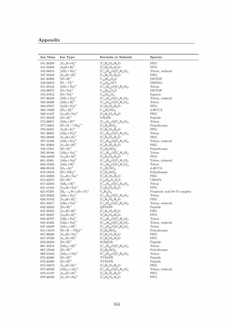
Appendix
Ion Mass Ion Type Formula or Subunit Species
541.26209 [A11B+K]+ [C2H4O]nH2O PEG
541.39463 [A9B+H]+ [C3H6O]nH2O PPG
543.38674 [AB7+Na]+ [C14H28O][C2H4O]n Triton, reduced
547.33242 [A12B+H]+ [C2H4O]nH2O PEG
547.40269 [M+H]+ C30H58O6S DDTDP
550.62853 [M− Cl]+ C38H80NCl DSDMA
551.35544 [AB7+Na]+ [C15H24O][C2H4O]n Triton
553.38972 [M+Na]+ C30H58O5S DDTDP
553.45912 [M+Na]+ C35H62O3 Irganox
557.40239 [AB7+Na]+ [C15H30O][C2H4O]n Triton, reduced
559.38406 [AB8+H]+ [C14H22O][C2H4O]n Triton
563.37657 [A9B+Na]+ [C3H6O]nH2O PPG
568.13506 [M3+H]+ C10H7NO3 4-HCCA
569.31437 [A12B+Na]+ [C2H4O]nH2O PEG
571.35622 [M+H]+ VSLPR Peptide
573.39971 [AB8+H]+ [C15H24O][C2H4O]n Triton
577.12631 [M+H− CH4]+ [C2H6SiO]8 Polysiloxane
579.35051 [A9B+K]+ [C3H6O]nH2O PPG
581.36601 [AB8+Na]+ [C14H22O][C2H4O]n Triton
585.28830 [A12B+K]+ [C2H4O]nH2O PEG
587.41296 [AB8+Na]+ [C14H28O][C2H4O]n Triton, reduced
591.35864 [A13B+H]+ [C2H4O]nH2O PEG
593.15761 [M+H]+ [C2H6SiO]8 Polysiloxane
595.38166 [AB8+Na]+ [C15H24O][C2H4O]n Triton
599.43649 [A10B+H]+ [C3H6O]nH2O PPG
601.42861 [AB8+Na]+ [C15H30O][C2H4O]n Triton, reduced
603.41028 [AB9+H]+ [C14H22O][C2H4O]n Triton
606.09149 [M3+K]+ C10H7NO3 4-HCCA
610.18416 [M+NH4]+ [C2H6SiO]8 Polysiloxane
613.34058 [A13B+Na]+ [C2H4O]nH2O PEG
615.40375 [M+H]+ C32H58N2O7S CHAPS
617.42593 [AB9+H]+ [C15H24O][C2H4O]n Triton
621.41844 [A10B+Na]+ [C3H6O]nH2O PPG
621.97291 [M6 −6 H+3Fe+O]+ C3H6O2 Propionic acid Fe-O complex
625.39222 [AB9+Na]+ [C14H22O][C2H4O]n Triton
629.31452 [A13B+K]+ [C2H4O]nH2O PEG
631.43917 [AB9+Na]+ [C14H28O][C2H4O]n Triton, reduced
633.32023 [M+H]+ QTIASN Peptide
635.38485 [A14B+H]+ [C2H4O]nH2O PEG
637.39237 [A10B+K]+ [C3H6O]nH2O PPG
639.40787 [AB9+Na]+ [C15H24O][C2H4O]n Triton
645.45482 [AB9+Na]+ [C15H30O][C2H4O]n Triton, reduced
647.43649 [AB10+H]+ [C14H22O][C2H4O]n Triton
651.14510 [M+H− CH4]+ [C2H6SiO]9 Polysiloxane
657.36680 [A14B+Na]+ [C2H4O]nH2O PEG
657.47836 [A11B+H]+ [C3H6O]nH2O PPG
659.38350 [M+H]+ SGIQVR Peptide
661.45214 [AB10+H]+ [C15H24O][C2H4O]n Triton
667.17640 [M+H]+ [C2H6SiO]9 Polysiloxane
669.41844 [AB10+Na]+ [C14H22O][C2H4O]n Triton
672.40390 [M+H]+ TVSLPR Peptide
672.40390 [M+H]+ TVSLPR Peptide
673.34073 [A14B+K]+ [C2H4O]nH2O PEG
675.46539 [AB10+Na]+ [C14H28O][C2H4O]n Triton, reduced
679.41107 [A15B+H]+ [C2H4O]nH2O PEG
679.46030 [A11B+Na]+ [C3H6O]nH2O PPG
164
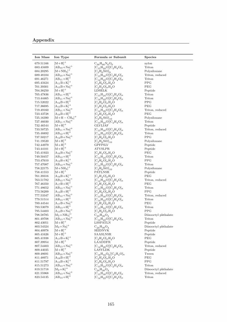
Appendix
Ion Mass Ion Type Formula or Subunit Species
679.51166 [M+H]+ C36H66N6O6 nylon
683.43409 [AB10+Na]+ [C15H24O][C2H4O]n Triton
684.20295 [M+NH4]+ [C2H6SiO]9 Polysiloxane
689.48104 [AB10+Na]+ [C15H30O][C2H4O]n Triton, reduced
691.46271 [AB11+H]+ [C14H22O][C2H4O]n Triton
695.43424 [A11B+K]+ [C3H6O]nH2O PPG
701.39301 [A15B+Na]+ [C2H4O]nH2O PEG
704.38250 [M+H]+ LDSELK Peptide
705.47836 [AB11+H]+ [C15H24O][C2H4O]n Triton
713.44465 [AB11+Na]+ [C14H22O][C2H4O]n Triton
715.52022 [A12B+H]+ [C3H6O]nH2O PPG
717.36695 [A15B+K]+ [C2H4O]nH2O PEG
719.49160 [AB11+Na]+ [C14H28O][C2H4O]n Triton, reduced
723.43728 [A16B+H]+ [C2H4O]nH2O PEG
725.16390 [M+H− CH4]+ [C2H6SiO]10 Polysiloxane
727.46030 [AB11+Na]+ [C15H24O][C2H4O]n Triton
732.46544 [M+H]+ GLVLIAF Peptide
733.50725 [AB11+Na]+ [C15H30O][C2H4O]n Triton, reduced
735.48892 [AB12+H]+ [C14H22O][C2H4O]n Triton
737.50217 [A12B+Na]+ [C3H6O]nH2O PPG
741.19520 [M+H]+ [C2H6SiO]10 Polysiloxane
742.44979 [M+H]+ GPFPILV Peptide
743.44101 [M+H]+ ATVSLPR Peptide
745.41923 [A16B+Na]+ [C2H4O]nH2O PEG
749.50457 [AB12+H]+ [C15H24O][C2H4O]n Triton
753.47610 [A12B+K]+ [C3H6O]nH2O PPG
757.47087 [AB12+Na]+ [C14H22O][C2H4O]n Triton
758.22175 [M+NH4]+ [C2H6SiO]10 Polysiloxane
758.41553 [M+H]+ PATLNSR Peptide
761.39316 [A16B+K]+ [C2H4O]nH2O PEG
763.51782 [AB12+Na]+ [C14H28O][C2H4O]n Triton, reduced
767.46350 [A17B+H]+ [C2H4O]nH2O PEG
771.48652 [AB12+Na]+ [C15H24O][C2H4O]n Triton
773.56209 [A13B+H]+ [C3H6O]nH2O PPG
777.53347 [AB12+Na]+ [C15H30O][C2H4O]n Triton, reduced
779.51514 [AB13+H]+ [C14H22O][C2H4O]n Triton
789.44544 [A17B+Na]+ [C2H4O]nH2O PEG
793.53079 [AB13+H]+ [C15H24O][C2H4O]n Triton
795.54403 [A13B+Na]+ [C3H6O]nH2O PPG
798.58785 [M2+NH4]+ C24H38O4 Diisooctyl phthalate
801.49708 [AB13+Na]+ [C14H22O][C2H4O]n Triton
802.43051 [M+H]+ LSSPATLN Peptide
803.54324 [M2+Na]+ C24H38O4 Diisooctyl phthalate
804.40978 [M+H]+ SEIDNVK Peptide
805.41626 [M+H]+ SAASLNSR Peptide
805.41938 [A17B+K]+ [C2H4O]nH2O PEG
807.39954 [M+H]+ LAADDFR Peptide
807.54403 [AB13+Na]+ [C14H28O][C2H4O]n Triton, reduced
809.44035 [M+H]+ LASYLDK Peptide
809.48691 [AB10+Na]+ [C18H34O6][C2H4O]n Tween
811.48971 [A18B+H]+ [C2H4O]nH2O PEG
811.51797 [A13B+K]+ [C3H6O]nH2O PPG
815.51273 [AB13+Na]+ [C15H24O][C2H4O]n Triton
819.51718 [M2+K]+ C24H38O4 Diisooctyl phthalate
821.55968 [AB13+Na]+ [C15H30O][C2H4O]n Triton, reduced
823.54135 [AB14+H]+ [C14H22O][C2H4O]n Triton
165
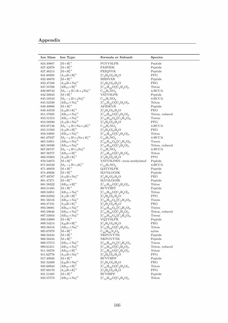
Appendix
Ion Mass Ion Type Formula or Subunit Species
824.49887 [M+H]+ PGVVSLPR Peptide
827.42978 [M+H]+ FASFIDK Peptide
827.46214 [M+H]+ PEIQNVK Peptide
831.60395 [A14B+H]+ [C3H6O]nH2O PPG
832.48870 [M+H]+ SISISVAR Peptide
833.47166 [A18B+Na]+ [C2H4O]nH2O PEG
837.55700 [AB14+H]+ [C15H24O][C2H4O]n Triton
839.09742 [M4 −2 H+K+2Na]+ C10H7NO3 4-HCCA
842.50943 [M+H]+ VATVSLPR Peptide
845.10543 [M4 −3 H+4Na]+ C10H7NO3 4-HCCA
845.52330 [AB14+Na]+ [C14H22O][C2H4O]n Triton
848.49886 [M+H]+ AFIDKVR Peptide
849.44559 [A18B+K]+ [C2H4O]nH2O PEG
851.57025 [AB14+Na]+ [C14H28O][C2H4O]n Triton, reduced
853.51313 [AB11+Na]+ [C18H34O6][C2H4O]n Tween
853.58590 [A14B+Na]+ [C3H6O]nH2O PPG
855.07136 [M4 −2 H+Na+2K]+ C10H7NO3 4-HCCA
855.51593 [A19B+H]+ [C2H4O]nH2O PEG
859.53895 [AB14+Na]+ [C15H24O][C2H4O]n Triton
861.07937 [M4 −3 H+3Na+K]+ C10H7NO3 4-HCCA
865.54951 [AB10+Na]+ [C22H42O6][C2H4O]n Tween
865.58590 [AB14+Na]+ [C15H30O][C2H4O]n Triton, reduced
867.08737 [M4 −4 H+5Na]+ C10H7NO3 4-HCCA
867.56757 [AB15+H]+ [C14H22O][C2H4O]n Triton
869.55983 [A14B+K]+ [C3H6O]nH2O PPG
870.54073 [M+H]+ VATVSLPRN−term·methylated Peptide
871.04530 [M4 −2 H+3K]+ C10H7NO3 4-HCCA
871.49959 [M+H]+ QATVSLPR Peptide
874.49926 [M+H]+ SLVNLGGSK Peptide
877.49787 [A19B+Na]+ [C2H4O]nH2O PEG
881.47271 [M+H]+ SLYGLGGSK Peptide
881.58322 [AB15+H]+ [C15H24O][C2H4O]n Triton
883.51485 [M+H]+ RVYVHPI Peptide
889.54951 [AB15+Na]+ [C14H22O][C2H4O]n Triton
889.64582 [A15B+H]+ [C3H6O]nH2O PPG
891.56516 [AB10+Na]+ [C24H44O6][C2H4O]n Tween
893.47181 [A19B+K]+ [C2H4O]nH2O PEG
893.58081 [AB10+Na]+ [C24H46O6][C2H4O]n Tween
895.59646 [AB15+Na]+ [C14H28O][C2H4O]n Triton, reduced
897.53934 [AB12+Na]+ [C18H34O6][C2H4O]n Tween
899.53089 [M+H]+ VQTVSLPR Peptide
899.54214 [A20B+H]+ [C2H4O]nH2O PEG
903.56516 [AB15+Na]+ [C15H24O][C2H4O]n Triton
905.67979 [M+H]+ C48H88N8O8 nylon
906.50434 [M+H]+ NKPGVYTK Peptide
906.50434 [M+H]+ NKPGVYTK Peptide
909.57573 [AB11+Na]+ [C22H42O6][C2H4O]n Tween
909.61211 [AB15+Na]+ [C15H30O][C2H4O]n Triton, reduced
911.59378 [AB16+H]+ [C14H22O][C2H4O]n Triton
911.62776 [A15B+Na]+ [C3H6O]nH2O PPG
917.49920 [M+H]+ RVYVHPF Peptide
921.52409 [A20B+Na]+ [C2H4O]nH2O PEG
925.60943 [AB16+H]+ [C15H24O][C2H4O]n Triton
927.60170 [A15B+K]+ [C3H6O]nH2O PPG
931.51485 [M+H]+ RVYIHPF Peptide
933.57573 [AB16+Na]+ [C14H22O][C2H4O]n Triton
166

Appendix
Ion Mass Ion Type Formula or Subunit Species
935.59138 [AB11+Na]+ [C24H44O6][C2H4O]n Tween
937.49802 [A20B+K]+ [C2H4O]nH2O PEG
937.60703 [AB11+Na]+ [C24H46O6][C2H4O]n Tween
939.62268 [AB16+Na]+ [C14H28O][C2H4O]n Triton, reduced
941.56556 [AB13+Na]+ [C18H34O6][C2H4O]n Tween
947.59138 [AB16+Na]+ [C15H24O][C2H4O]n Triton
947.68768 [A16B+H]+ [C3H6O]nH2O PPG
950.47305 [M+H]+ YVNWIQQ Peptide
953.60194 [AB12+Na]+ [C22H42O6][C2H4O]n Tween
953.63833 [AB16+Na]+ [C15H30O][C2H4O]n Triton, reduced
955.62000 [AB17+H]+ [C14H22O][C2H4O]n Triton
969.63565 [AB17+H]+ [C15H24O][C2H4O]n Triton
969.66963 [A16B+Na]+ [C3H6O]nH2O PPG
973.53129 [M+H]+ IEISELNR Peptide
977.60194 [AB17+Na]+ [C14H22O][C2H4O]n Triton
979.50949 [M+H]+ GTSYPDVLK Peptide
979.61759 [AB12+Na]+ [C24H44O6][C2H4O]n Tween
981.63324 [AB12+Na]+ [C24H46O6][C2H4O]n Tween
983.64889 [AB17+Na]+ [C14H28O][C2H4O]n Triton, reduced
985.59177 [AB14+Na]+ [C18H34O6][C2H4O]n Tween
985.64356 [A16B+K]+ [C3H6O]nH2O PPG
991.61759 [AB17+Na]+ [C15H24O][C2H4O]n Triton
994.15551 [M5 −H2O−2 H+3Na]+ C10H7NO3 4-HCCA
995.51966 [M+H]+ IKEWYEK Peptide
997.62816 [AB13+Na]+ [C22H42O6][C2H4O]n Tween
997.66454 [AB17+Na]+ [C15H30O][C2H4O]n Triton, reduced
999.64621 [AB18+H]+ [C14H22O][C2H4O]n Triton
167

Appendix
LC-MS Adducts, Losses, and Replacements
List of potential gains, losses, and replacements in positive ion mode LC-ESI-MS.
The list is adapted from Keller et al. [110]. The exact mass difference, ion type,
reaction, and potential origin of the compound is provided.
Mass Difference Ion type Reaction Origin
14.01565 [A: [C3H6ON]↔ [C2H4ON]]+ C3H6ON −−⇀↽−− C2H4ON acrylamide/iodoacetamide
43.94948442[A:79Br↔Cl
]+ 79Br −−⇀↽−− Cl halogen exchange
52.9152631[A:79Br↔CN
]+ 79Br −−⇀↽−− CN halogen exchange
77.9105121[A:79Br↔H
]+ 79Br −−⇀↽−− H halogen exchange
61.9155971[A:79Br↔OH
]+ 79Br −−⇀↽−− OH halogen exchange
45.94743792[A:81Br↔Cl
]+ 81Br −−⇀↽−− Cl halogen exchange
54.9132166[A:81Br↔CN
]+ 81Br −−⇀↽−− CN halogen exchange
79.9084656[A:81Br↔H
]+ 81Br −−⇀↽−− H halogen exchange
63.9135506[A:81Br↔OH
]+ 81Br −−⇀↽−− OH halogen exchange
37.989162 [A:2CN↔2COOH]+ 2 CN −−⇀↽−− 2 COOH nitrile compounds
8.96577868 [A:Cl↔CN]+ Cl −−⇀↽−− CN halogen exchange
33.96102768 [A:Cl↔H]+ Cl −−⇀↽−− H halogen exchange
17.96611268 [A:Cl↔OH]+ Cl −−⇀↽−− OH halogen exchange
18.994581 [A:CN↔COO]+ CN −−⇀↽−− COO nitrile compounds
24.995249 [A:CN↔H]+ CN −−⇀↽−− H nitrile compounds
7.00467078 [A:F↔CN]+ F −−⇀↽−− CN halogen exchange
17.99057822 [A:F↔H]+ F −−⇀↽−− H halogen exchange
1.99566322 [A:F↔OH]+ F −−⇀↽−− OH halogen exchange
91.93562072 [A:I↔Cl]+ I −−⇀↽−− Cl halogen exchange
100.9013994 [A:I↔CN]+ I −−⇀↽−− CN halogen exchange
125.8966484 [A:I↔H]+ I −−⇀↽−− H halogen exchange
109.9017334 [A:I↔OH]+ I −−⇀↽−− OH halogen exchange
37.955881[A:K+↔H+
]+K+ −−⇀↽−− H+ salt adduct
20.929332[A:K+↔NH+
4
]+K+ −−⇀↽−− NH4
+ salt adduct
21.981944[A:Na+↔H+
]+Na+ −−⇀↽−− H+ salt adduct
15.973937[A:Na+↔K+
]+Na+ −−⇀↽−− K+ salt adduct
4.955395[A:Na+↔NH+
4
]+Na+ −−⇀↽−− NH4
+ salt adduct
17.026549[A:NH+
4 ↔H+]+
NH4+ −−⇀↽−− H+ salt adduct
29.97418 [A:NO2↔NH2]+ NO2−−⇀↽−− NH2 nitro compounds
13.979265 [A:O↔2H]+ O −−⇀↽−− 2 H Oxidation
0.984016 [A:OH↔NH2]+ OH −−⇀↽−− NH2 de-amidation
15.977156 [A:S↔O]+ S −−⇀↽−− O sulfur compounds
28.006148 [A−2N]+ nitrogen loss
63.998286 [A−CH3SOH]+ oxidized methionines
33.021464 [A−NH2OH]+ hydroxamic acids
29.997989 [A−NO]+ nitroso compounds
2.01565 [A±2H]+ double bond formation
31.98983 [A±2O]+ oxygen loss
305.068158 [A±C10O6N3SH15]+ glutathione+o-water
307.083808 [A±C10O6N3SH17]+ glutathione
289.073243 [A±C10O5N3SH15]+ glutathione-water
291.095419 [A±C11O8NH17]+ sialic acid
309.105984 [A±C11O9NH19]+ sialic acid
168

Appendix
Mass Difference Ion type Reaction Origin
324.10565 [A±C12O10H20]+ sucrose-water
342.116215 [A±C12O11H22]+ sucrose
28.0313 [A±C2H4]+ natural alkane chains
42.04695 [A±C3H6]+ propylation
56.0626 [A±C4H8]+ butylation
146.05791 [A±C6O4H10]+ deoxy-hexose-water
162.052825 [A±C6O5H10]+ hexose-water
164.068475 [A±C6O5H12]+ deoxy-hexose-water
180.06339 [A±C6O6H12]+ hexose
176.03209 [A±C6O6H8]+ glucuronic acid
194.042655 [A±C6O7H10]+ glucuronic acid
203.079374 [A±C8O5NH13]+ n-acetylhexoseamine
221.089939 [A±C8O6NH15]+ n-acetylhexoseamine
14.01565 [A±CH2]+ methylation
27.994915 [A±CO]+ carbon monoxide
58.00548 [A±CO2CH2]+ ester
43.98983 [A±CO2]+ decarboxylation
42.010565 [A±COCH2]+ acetyl loss/gain
43.005814 [A±CONH]+ acyl amide loss/gain
33.987721 [A±H2S]+ sulfur compounds
97.976897 [A±H3PO4]+ phosphorous compounds
18.010565 [A±H2O]+ water addition/loss
97.967381 [A±H2SO4]+ sulfur compounds
27.010899 [A±HCN]+ nitrile compounds
17.026549 [A±NH3]+ ammonium adduct
15.994915 [A±O]+ oxidation/reduction
31.972071 [A±S]+ sulfur compounds
47.966986 [A±SO]+ sulfur compounds
63.961901 [A±SO2]+ sulfur compounds
79.956816 [A±SO3]+ sulfur compounds
40.0313 [A+(C3H6O−H2O)]+ acetone condensation
58.041865 [A+C3H6O]+ acetone condensation
169


References
[1] Ewa Urbanczyk-Wochniak, Alexander Luedemann, Joachim Kopka, Joachim Selbig, Ute Roessner-Tunali,Lothar Willmitzer, and Alisdair R Fernie. Parallel analysis of transcript and metabolic profiles: a newapproach in systems biology. EMBO reports, 4(10):989–93, October 2003.
[2] C H Waddington. The epigenotype. Endeavour, 1:18–20, 1942.
[3] Haleem J Issaq, Que N Van, Timothy J Waybright, Gary M Muschik, and Timothy D Veenstra. Analyticaland statistical approaches to metabolomics research. Journal of separation science, 32(13):2183–99, July2009.
[4] Tobias Kind, Kwang-Hyeon Liu, Do Yup Lee, Brian DeFelice, John K Meissen, and Oliver Fiehn. Lipid-Blast in silico tandem mass spectrometry database for lipid identification. Nature methods, 10(8):755–8,August 2013.
[5] Manish Sud, Eoin Fahy, and Shankar Subramaniam. Template-based combinatorial enumeration of virtualcompound libraries for lipids. Journal of Cheminformatics, 4(1):23, 2012.
[6] Scott Boyer, Catrin Hasselgren Arnby, Lars Carlsson, James Smith, Viktor Stein, and Robert C Glen.Reaction site mapping of xenobiotic biotransformations. Journal of chemical information and modeling,47(2):583–90, 2007.
[7] Bryson D Bennett, Elizabeth H Kimball, Melissa Gao, Robin Osterhout, Stephen J Van Dien, andJoshua D Rabinowitz. Absolute metabolite concentrations and implied enzyme active site occupancyin Escherichia coli. Nature chemical biology, 5(8):593–9, August 2009.
[8] Neepa Y Choksi, Gloria D Jahnke, Cathy St Hilaire, and Michael Shelby. Role of thyroid hormones inhuman and laboratory animal reproductive health. Birth defects research. Part B, Developmental andreproductive toxicology, 68(6):479–91, December 2003.
[9] E Grouzmann, M Fathi, M Gillet, a de Torrente, C Cavadas, H Brunner, and T Buclin. Disappearance rateof catecholamines, total metanephrines, and neuropeptide Y from the plasma of patients after resectionof pheochromocytoma. Clinical chemistry, 47(6):1075–82, June 2001.
[10] James R Lupski. Genetics. Genome mosaicism–one human, multiple genomes. Science (New York, N.Y.),341(6144):358–9, July 2013.
[11] Xiaojun Feng, Xin Liu, Qingming Luo, and Bi-Feng Liu. Mass spectrometry in systems biology: anoverview. Mass spectrometry reviews, 27(6):635–60, 2008.
[12] Katja Dettmer, P.A. Aronov, and B.D. Hammock. Mass spectrometry-based metabolomics. Mass Spec-trometry Reviews, 26(1):51, 2007.
[13] Vladimir Shulaev. Metabolomics technology and bioinformatics. Briefings in bioinformatics, 7(2):128–39,June 2006.
[14] Oliver Fiehn. Metabolomics–the link between genotypes and phenotypes. Plant molecular biology, 48(1-2):155–71, January 2002.
[15] David I Ellis, Warwick B Dunn, Julian L Griffin, J William Allwood, and Royston Goodacre. Metabolicfingerprinting as a diagnostic tool. Pharmacogenomics, 8(9):1243–66, September 2007.
171

REFERENCES
[16] David S Wishart, Timothy Jewison, An Chi Guo, Michael Wilson, Craig Knox, Yifeng Liu, YannickDjoumbou, Rupasri Mandal, Farid Aziat, Edison Dong, Souhaila Bouatra, Igor Sinelnikov, David Arndt,Jianguo Xia, Philip Liu, Faizath Yallou, Trent Bjorndahl, Rolando Perez-Pineiro, Roman Eisner, Felic-ity Allen, Vanessa Neveu, Russ Greiner, and Augustin Scalbert. HMDB 3.0–The Human MetabolomeDatabase in 2013. Nucleic acids research, 41:801–807, 2012.
[17] Tobias Kind, Martin Scholz, and Oliver Fiehn. How large is the metabolome? A critical analysis of dataexchange practices in chemistry. PloS one, 4(5):e5440, January 2009.
[18] Gary J Patti, Oscar Yanes, and Gary Siuzdak. Innovation: Metabolomics: the apogee of the omics trilogy.Nature reviews. Molecular cell biology, 13(4):263–9, April 2012.
[19] Royston Goodacre. An overflow of. . . what else but metabolism! Metabolomics, 6(1):1–2, February 2010.
[20] Oliver Fiehn, Don Robertson, Jules Griffin, Mariet Werf, Basil Nikolau, Norman Morrison, Lloyd W.Sumner, Roy Goodacre, Nigel W. Hardy, Chris Taylor, Jennifer Fostel, Bruce Kristal, Rima Kaddurah-Daouk, Pedro Mendes, Ben Ommen, John C. Lindon, and Susanna-Assunta Sansone. The metabolomicsstandards initiative (MSI). Metabolomics, 3(3):175–178, August 2007.
[21] Jocelyn Kaiser. Proteomics. Public-private group maps out initiatives. Science (New York, N.Y.), 296(5569):827, May 2002.
[22] Souhaila Bouatra, Farid Aziat, Rupasri Mandal, An Chi Guo, Michael R. Wilson, Craig Knox, Trent C.Bjorndahl, Ramanarayan Krishnamurthy, Fozia Saleem, Philip Liu, Zerihun T. Dame, Jenna Poelzer,Jessica Huynh, Faizath S. Yallou, Nick Psychogios, Edison Dong, Ralf Bogumil, Cornelia Roehring, andDavid S. Wishart. The Human Urine Metabolome. PLoS ONE, 8(9):e73076, September 2013.
[23] Kenneth Haug, Reza M Salek, Pablo Conesa, Janna Hastings, Paula de Matos, Mark Rijnbeek, Te-jasvi Mahendraker, Mark Williams, Steffen Neumann, Philippe Rocca-Serra, Eamonn Maguire, AlejandraGonzalez-Beltran, Susanna-Assunta Sansone, Julian L Griffin, and Christoph Steinbeck. MetaboLights–an open-access general-purpose repository for metabolomics studies and associated meta-data. Nucleicacids research, 41(Database issue):D781–6, January 2013.
[24] Manhoi Hur, Alexis Ann Campbell, Marcia Almeida-de Macedo, Ling Li, Nick Ransom, Adarsh Jose,Matt Crispin, Basil J Nikolau, and Eve Syrkin Wurtele. A global approach to analysis and interpretationof metabolic data for plant natural product discovery. Natural product reports, 30:565–83, 2013.
[25] Nikolas Kessler, Heiko Neuweger, Anja Bonte, Georg Langenkamper, Karsten Niehaus, Tim W Nattkem-per, and Alexander Goesmann. MeltDB 2.0-advances of the metabolomics software system. Bioinformatics(Oxford, England), 29(19):2452–2459, August 2013.
[26] Lionel Blanchet, Agnieszka Smolinska, Amos Attali, Marcel P Stoop, Kirsten Am Ampt, Hans van Aken,Ernst Suidgeest, Tinka Tuinstra, Sybren S Wijmenga, Theo Luider, and Lutgarde Mc Buydens. Fusion ofmetabolomics and proteomics data for biomarkers discovery: case study on the experimental autoimmuneencephalomyelitis. BMC bioinformatics, 12(1):254, June 2011.
[27] J E MacNair, K C Lewis, and J W Jorgenson. Ultrahigh-pressure reversed-phase liquid chromatographyin packed capillary columns. Analytical chemistry, 69(6):983–9, March 1997.
[28] Kamlesh D Patel, Anton D Jerkovich, Jason C Link, and James W Jorgenson. In-depth characterizationof slurry packed capillary columns with 1.0-microm nonporous particles using reversed-phase isocraticultrahigh-pressure liquid chromatography. Analytical chemistry, 76(19):5777–86, October 2004.
[29] John V Seeley and Stacy K Seeley. Multidimensional gas chromatography: fundamental advances andnew applications. Analytical chemistry, 85(2):557–78, January 2013.
[30] Agnieszka Smolinska, Lionel Blanchet, Lutgarde M C Buydens, and Sybren S Wijmenga. NMR andpattern recognition methods in metabolomics: From data acquisition to biomarker discovery: A review.Analytica chimica acta, 750:82–97, October 2012.
[31] Mohamed a. Farag, Andrea Porzel, Jurgen Schmidt, and Ludger a. Wessjohann. Metabolite profilingand fingerprinting of commercial cultivars of Humulus lupulus L. (hop): a comparison of MS and NMRmethods in metabolomics. Metabolomics, 8(3):492–507, August 2011.
[32] K. a. Aliferis and S. Jabaji. 1H NMR and GC-MS metabolic fingerprinting of developmental stages ofRhizoctonia solani sclerotia. Metabolomics, 6(1):96–108, September 2009.
[33] Arjen Lommen, Arjen Gerssen, J. Efraim Oosterink, Harrie J. Kools, Ainhoa Ruiz-Aracama, Ruud J. B.Peters, and Hans G. J. Mol. Ultra-fast searching assists in evaluating sub-ppm mass accuracy enhancementin U-HPLC/Orbitrap MS data. Metabolomics : Official journal of the Metabolomic Society, 7(1):15–24,March 2011.
172

REFERENCES
[34] Jurre J Kamphorst, Jing Fan, Wenyun Lu, Eileen White, and Joshua D Rabinowitz. Liquidchromatography-high resolution mass spectrometry analysis of fatty acid metabolism. Analytical chem-istry, 83(23):9114–22, December 2011.
[35] Haitao Lv. Mass spectrometry-based metabolomics towards understanding of gene functions with a di-versity of biological contexts. Mass spectrometry reviews, 32(2):118–28, 2012.
[36] Sofia Moco, Jacques Vervoort, Raoul J. Bino, Ric C.H. De Vos, and Raoul Bino. Metabolomics technologiesand metabolite identification. TrAC Trends in Analytical Chemistry, 26(9):855–866, October 2007.
[37] Bin Zhou, Jun Feng Xiao, Leepika Tuli, and Habtom W Ressom. LC-MS-based metabolomics. MolecularbioSystems, 8(2):470–81, February 2012.
[38] Monya Baker. Metabolomics: from small molecules to big ideas. Nature Methods, 8(2):117–121, February2011.
[39] Susan D Richardson. Environmental mass spectrometry: emerging contaminants and current issues.Analytical chemistry, 82(12):4742–74, June 2010.
[40] J William Allwood and Royston Goodacre. An introduction to liquid chromatography-mass spectrometryinstrumentation applied in plant metabolomic analyses. Phytochemical analysis : PCA, 21(1):33–47,2010.
[41] Ken Webb, Tony Bristow, and Mike Sargent. Methodology for Accurate Mass Measurement of SmallMolecules Best Practice Guide. Technical report, LGC Ltd., 2004.
[42] Maud M. Koek, Renger H. Jellema, Jan van der Greef, Albert C. Tas, and Thomas Hankemeier.Quantitative metabolomics based on gas chromatography mass spectrometry: status and perspectives.Metabolomics : Official journal of the Metabolomic Society, 7(3):307–328, September 2011.
[43] Liang Cui, Yie Hou Lee, Yadunanda Kumar, Fengguo Xu, Kun Lu, Eng Eong Ooi, Steven R. Tannenbaum,and Choon Nam Ong. Serum Metabolome and Lipidome Changes in Adult Patients with Primary DengueInfection. PLoS Neglected Tropical Diseases, 7(8):e2373, August 2013.
[44] Carsten Denkert, Jan Budczies, Tobias Kind, Wilko Weichert, Peter Tablack, Jalid Sehouli, Silvia Nies-porek, Dominique Konsgen, Manfred Dietel, and Oliver Fiehn. Mass spectrometry-based metabolic pro-filing reveals different metabolite patterns in invasive ovarian carcinomas and ovarian borderline tumors.Cancer research, 66(22):10795–804, November 2006.
[45] Masahiro Sugimoto, David T Wong, Akiyoshi Hirayama, Tomoyoshi Soga, and Masaru Tomita. Capillaryelectrophoresis mass spectrometry-based saliva metabolomics identified oral, breast and pancreatic cancer-specific profiles. Metabolomics : Official journal of the Metabolomic Society, 6(1):78–95, March 2010.
[46] Ghaniah Hassan-Smith, Graham R Wallace, Michael R Douglas, and Alexandra J Sinclair. The role ofmetabolomics in neurological disease. Journal of neuroimmunology, 248(1-2):48–52, July 2012.
[47] Elizabeth J Want, Ian D Wilson, Helen Gika, Georgios Theodoridis, Robert S Plumb, John Shockcor,Elaine Holmes, and Jeremy K Nicholson. Global metabolic profiling procedures for urine using UPLC-MS.Nature protocols, 5(6):1005–18, January 2010.
[48] Xinjie Zhao, Jens Fritsche, Jiangshan Wang, Jing Chen, Kilian Rittig, Philippe Schmitt-Kopplin, AndreasFritsche, Hans-Ulrich Haring, Erwin D. Schleicher, Guowang Xu, and Rainer Lehmann. Metabonomicfingerprints of fasting plasma and spot urine reveal human pre-diabetic metabolic traits. Metabolomics,6(3):362–374, March 2010.
[49] Anna Floegel, Norbert Stefan, Zhonghao Yu, Kristin Muhlenbruch, Dagmar Drogan, Hans-Georg Joost,Andreas Fritsche, Hans-Ulrich Haring, Martin Hrabe de Angelis, Annette Peters, Michael Roden, CorneliaPrehn, Rui Wang-Sattler, Thomas Illig, Matthias B Schulze, Jerzy Adamski, Heiner Boeing, and TobiasPischon. Identification of serum metabolites associated with risk of type 2 diabetes using a targetedmetabolomic approach. Diabetes, 62(2):639–48, February 2013.
[50] Fatima a. Nasrallah, Vladimir J. Balcar, and Caroline Rae. A metabonomic study of inhibition of GABAuptake in the cerebral cortex. Metabolomics, 6(1):67–77, August 2009.
[51] Rima Kaddurah-Daouk, Rebecca A Baillie, Hongjie Zhu, Zhao-Bang Zeng, Michelle M Wiest, Uyen ThaoNguyen, Steven M Watkins, and Ronald M Krauss. Lipidomic analysis of variation in response to simvas-tatin in the Cholesterol and Pharmacogenetics Study. Metabolomics : Official journal of the MetabolomicSociety, 6(2):191–201, June 2010.
173
REFERENCES
[52] Susan Schiavo Bird, Vasant R Marur, Matthew J Sniatynski, Heather K Greenberg, and Bruce S Kristal.Serum lipidomics profiling using LC-MS and high-energy collisional dissociation fragmentation: focus ontriglyceride detection and characterization. Analytical chemistry, 83(17):6648–57, September 2011.
[53] Todd R Sandrin, Jason E Goldstein, and Stephanie Schumaker. MALDI TOF MS profiling of bacteria atthe strain level: a review. Mass spectrometry reviews, 32(3):188–217, 2012.
[54] Jean-Philippe Lavigne, Paula Espinal, Catherine Dunyach-Remy, Nourredine Messad, Alix Pantel, andAlbert Sotto. Mass spectrometry: a revolution in clinical microbiology? Clinical chemistry and laboratorymedicine : CCLM / FESCC, pages 1–14, October 2012.
[55] M. Wink. Plant breeding: importance of plant secondary metabolites for protection against pathogensand herbivores. Theoretical and Applied Genetics, 75(2):225–233, January 1988.
[56] O Fiehn, J Kopka, P Dormann, T Altmann, R N Trethewey, and L Willmitzer. Metabolite profiling forplant functional genomics. Nature biotechnology, 18(11):1157–61, November 2000.
[57] Patricia M Cano, Emilien L Jamin, Souria Tadrist, Pascal Bourdaud’hui, Michel Pean, Laurent De-brauwer, Isabelle P Oswald, Marcel Delaforge, and Olivier Puel. New untargeted metabolic profiling com-bining mass spectrometry and isotopic labeling: application on Aspergillus fumigatus grown on wheat.Analytical chemistry, 85(17):8412–20, September 2013.
[58] Ric C H De Vos, Sofia Moco, Arjen Lommen, Joost J B Keurentjes, Raoul J Bino, and Robert D Hall.Untargeted large-scale plant metabolomics using liquid chromatography coupled to mass spectrometry.Nature protocols, 2(4):778–91, January 2007.
[59] Mark R. Viant and Ulf Sommer. Mass spectrometry based environmental metabolomics: a primer andreview. Metabolomics, 9(S1):144–158, March 2012.
[60] Atsushi Ishihara, Fumio Matsuda, Hisashi Miyagawa, and Kyo Wakasa. Metabolomics for metabolicallymanipulated plants: effects of tryptophan overproduction. Metabolomics, 3(3):319–334, September 2007.
[61] Yaniv Semel, Nicolas Schauer, Ute Roessner, Dani Zamir, and Alisdair Robert Fernie. Metabolite analysisfor the comparison of irrigated and non-irrigated field grown tomato of varying genotype. Metabolomics,3(3):289–295, June 2007.
[62] Georgios Theodoridis, Helen Gika, Pietro Franceschi, Lorenzo Caputi, Panagiotis Arapitsas, MattiasScholz, Domenico Masuero, Ron Wehrens, Urska Vrhovsek, and Fulvio Mattivi. LC-MS based globalmetabolite profiling of grapes: solvent extraction protocol optimisation. Metabolomics, 8(2):175–185,March 2011.
[63] Yozo Okazaki, Yukiko Kamide, Masami Yokota Hirai, and Kazuki Saito. Plant lipidomics based on hy-drophilic interaction chromatography coupled to ion trap time-of-flight mass spectrometry. Metabolomics: Official journal of the Metabolomic Society, 9(Suppl 1):121–131, March 2013.
[64] Jiangjiang Liu, He Wang, R Graham Cooks, and Zheng Ouyang. Leaf spray: direct chemical analysisof plant material and living plants by mass spectrometry. Analytical chemistry, 83(20):7608–13, October2011.
[65] Peter W Carr, Dwight R Stoll, and Xiaoli Wang. Perspectives on recent advances in the speed of high-performance liquid chromatography. Analytical chemistry, 83(6):1890–900, March 2011.
[66] Tania Portoles, Elena Pitarch, Francisco J Lopez, Felix Hernandez, and Wilfried M A Niessen. Use ofsoft and hard ionization techniques for elucidation of unknown compounds by gas chromatography/time-of-flight mass spectrometry. Data Processing, 25:1589–1599, 2011.
[67] Bhagwat Prasad, Amit Garg, Hardik Takwani, and Saranjit Singh. Metabolite identification by liquidchromatography-mass spectrometry. TrAC Trends in Analytical Chemistry, 30(2):360–387, February2011.
[68] Sara Forcisi, Franco Moritz, Basem Kanawati, Dimitrios Tziotis, Rainer Lehmann, and Philippe Schmitt-Kopplin. Liquid chromatography-mass spectrometry in metabolomics research: Mass analyzers in ultrahigh pressure liquid chromatography coupling. Journal of chromatography. A, 1292:51–65, April 2013.
[69] John Draper, Amanda J. Lloyd, Royston Goodacre, and Manfred Beckmann. Flow infusion electro-spray ionisation mass spectrometry for high throughput, non-targeted metabolite fingerprinting: a review.Metabolomics, 9(S1):4–29, July 2012.
[70] Jurgen Hartler, Ravi Tharakan, Harald C Kofeler, David R Graham, and Gerhard G Thallinger. Bioinfor-matics tools and challenges in structural analysis of lipidomics MS/MS data. Briefings in bioinformatics,14(3):375–90, May 2013.
174

REFERENCES
[71] David G Watson. A Rough Guide to Metabolite Identification Using High Resolution Liquid Chro-matography Mass Spectrometry in Metabolomic Profiling in Metazoans. Computational and structuralbiotechnology journal, 4(January):e201301005, January 2013.
[72] Phil Price. Standard definitions of terms relating to mass spectrometry. Journal of the American Societyfor Mass Spectrometry, 2(4):336–348, August 1991.
[73] Ryo Taguchi, Mashahiro Nishijima, and Takao Shimizu. Basic analytical systems for lipidomics by massspectrometry in Japan. Methods in Enzymology, 432:185–211, 2007.
[74] Ambrose Furey, Merisa Moriarty, Vaishali Bane, Brian Kinsella, and Mary Lehane. Ion suppression; Acritical review on causes, evaluation, prevention and applications. Talanta, 115:104–22, October 2013.
[75] Thomas M Annesley. Ion suppression in mass spectrometry. Clinical Chemistry, 49:1041–1044, 2003.
[76] WH McFadden and EA Day. Scan Rate Considerations in Combined Gas Chromatography-Mass Spec-trometry. Analytical Chemistry, 36(12):2362–2363, 1964.
[77] IUPAC. IUPAC Compendium of Chemical Terminology. IUPAC, Research Triagle Park, NC, June 2009.ISBN 0-9678550-9-8.
[78] Michael P Balogh and Waters Corp. Debating Resolution and Mass Accuracy. Journal of the AmericanSociety for Mass Spectrometry, 17(3), 2004.
[79] Gaetan Glauser, Nathalie Veyrat, Bertrand Rochat, Jean-Luc Wolfender, and Ted C J Turlings. Ultra-high pressure liquid chromatography-mass spectrometry for plant metabolomics: a systematic comparisonof high-resolution quadrupole-time-of-flight and single stage Orbitrap mass spectrometers. Journal ofchromatography. A, 1292:151–9, May 2013.
[80] Jeonghoon Lee and Peter T a Reilly. Limitation of Time-of-Flight Resolution in the Ultra High MassRange. Analytical chemistry, pages 5–7, July 2011.
[81] Warwick B Dunn. Current trends and future requirements for the mass spectrometric investigation ofmicrobial, mammalian and plant metabolomes. Physical Biology, 5:011001, 2008.
[82] Seongho Kim, Imhoi Koo, Aiqin Fang, and Xiang Zhang. Smith-Waterman peak alignment for comprehen-sive two-dimensional gas chromatography-mass spectrometry. BMC bioinformatics, 12(1):235, January2011.
[83] Miquel Rojas-Cherto, Julio E Peironcely, Piotr T Kasper, Justin J J van der Hooft, Ric C H de Vos,Rob Vreeken, Thomas Hankemeier, and Theo Reijmers. Metabolite Identification Using AutomatedComparison of High-Resolution Multistage Mass Spectral Trees. Analytical chemistry, June 2012.
[84] Stephen Stein. Mass spectral reference libraries: an ever-expanding resource for chemical identification.Analytical chemistry, 84(17):7274–82, September 2012.
[85] Jiyang Zhang, Jie Ma, Wei Zhang, Changming Xu, Yunping Zhu, and Hongwei Xie. FTDR 2.0: a tool toachieve sub-ppm level recalibrated accuracy in routine LC-MS analysis. July 2013. ISBN 8673184576.
[86] Helen G Gika, Georgios a Theodoridis, Robert S Plumb, and Ian D Wilson. Current practice of liquidchromatography-mass spectrometry in metabolomics and metabonomics. Journal of pharmaceutical andbiomedical analysis, 87:12–25, January 2014.
[87] Igor Nikolskiy, Nathaniel G Mahieu, Ying-Jr Chen, Ralf Tautenhahn, and Gary J Patti. An untargetedmetabolomic workflow to improve structural characterization of metabolites. Analytical chemistry, 85(16):7713–9, August 2013.
[88] Tairo Ogura, Takeshi Bamba, and Eiichiro Fukusaki. Development of a practical metabolite identificationtechnique for non-targeted metabolomics. Journal of Chromatography A, pages 1–7, May 2013.
[89] Esther Sl Chong, Tony K McGhie, Julian a Heyes, and Kathryn M Stowell. Metabolite profiling andquantification of phytochemicals in potato extracts using ultra high performance liquid chromatography-mass spectrometry. Journal of the science of food and agriculture, June 2013.
[90] Julio E Peironcely, Miguel Rojas-Cherto, Albert Tas, Rob Vreeken, Theo Reijmers, Leon Coulier, andThomas Hankemeier. Automated pipeline for de novo metabolite identification using mass-spectrometry-based metabolomics. Analytical chemistry, 85(7):3576–83, April 2013.
[91] Lars J Kangas, Thomas O Metz, Giorgis Isaac, Brian T Schrom, Bojana Ginovska-Pangovska, LuningWang, Li Tan, Robert R Lewis, and John H Miller. In silico identification software (ISIS): a machine
175

REFERENCES
learning approach to tandem mass spectral identification of lipids. Bioinformatics (Oxford, England), 28(13):1705–13, July 2012.
[92] Karen W Phinney, Guillaume Ballihaut, Mary Bedner, Brandi S Benford, Johanna E Camara, Steven JChristopher, W Clay Davis, Nathan G Dodder, Gauthier Eppe, Brian E Lang, Stephen E Long, Mark SLowenthal, Elizabeth a McGaw, Karen E Murphy, Bryant C Nelson, Jocelyn L Prendergast, Jessica LReiner, Catherine a Rimmer, Lane C Sander, Michele M Schantz, Katherine E Sharpless, Lorna TSniegoski, Susan S-C Tai, Jeanice B Thomas, Thomas W Vetter, Michael J Welch, Stephen a Wise,Laura J Wood, William F Guthrie, Charles R Hagwood, Stefan D Leigh, James H Yen, Nien-Fan Zhang,Madhu Chaudhary-Webb, Huiping Chen, Zia Fazili, Donna J LaVoie, Leslie F McCoy, Shahzad S Momin,Neelima Paladugula, Elizabeth C Pendergrast, Christine M Pfeiffer, Carissa D Powers, Daniel Rabinowitz,Michael E Rybak, Rosemary L Schleicher, Bridgette M H Toombs, Mary Xu, Mindy Zhang, and Arthur LCastle. Development of a Standard Reference Material for metabolomics research. Analytical chemistry,85(24):11732–8, December 2013.
[93] Marie Brown, Warwick B. Dunn, David I. Ellis, Royston Goodacre, Julia Handl, Joshua D. Knowles, SteveOHagan, Irena Spasic, and Douglas B. Kell. A metabolome pipeline: from concept to data to knowledge.Metabolomics, 1(1):39–51, March 2005.
[94] Patrick G a Pedrioli, Jimmy K Eng, Robert Hubley, Mathijs Vogelzang, Eric W Deutsch, Brian Raught,Brian Pratt, Erik Nilsson, Ruth H Angeletti, Rolf Apweiler, Kei Cheung, Catherine E Costello, HenningHermjakob, Sequin Huang, Randall K Julian, Eugene Kapp, Mark E McComb, Stephen G Oliver, GilbertOmenn, Norman W Paton, Richard Simpson, Richard Smith, Chris F Taylor, Weimin Zhu, and RuediAebersold. A common open representation of mass spectrometry data and its application to proteomicsresearch. Nature biotechnology, 22(11):1459–66, November 2004.
[95] Sandra Orchard, Luisa Montechi-Palazzi, Eric W Deutsch, Pierre-Alain Binz, Andrew R Jones, NormanPaton, Angel Pizarro, David M Creasy, Jerome Wojcik, and Henning Hermjakob. Five years of progress inthe Standardization of Proteomics Data 4th Annual Spring Workshop of the HUPO-Proteomics StandardsInitiative April 23-25, 2007 Ecole Nationale Superieure (ENS), Lyon, France. Proteomics, 7(19):3436–40,October 2007.
[96] E. Deutsch. mzML: a single, unifying data format for mass spectrometer output. Proteomics, 8(14):2776–2777, 2008.
[97] Eric W Deutsch. File formats commonly used in mass spectrometry proteomics. Molecular & cellularproteomics : MCP, (1):1–32, September 2012.
[98] R Rew and G Davis. NetCDF: an interface for scientific data access. IEEE Computer Graphics andApplications, 10:76–82, 1990.
[99] Sandra Orchard. Data standardization and sharing-the work of the HUPO-PSI. Biochimica et biophysicaacta, 1844(1 Pt A):82–7, January 2014.
[100] Julian L Griffin and Christoph Steinbeck. So what have data standards ever done for us? The view frommetabolomics. Genome medicine, 2(6):38, January 2010.
[101] Shaji Krishnan, Jack T W E Vogels, Leon Coulier, Richard C Bas, Margriet W B Hendriks, ThomasHankemeier, and Uwe Thissen. Instrument and process independent binning and baseline correctionmethods for liquid chromatography-high resolution-mass spectrometry deconvolution. Analytica chimicaacta, 740:12–9, August 2012.
[102] Peijuan Zhu, Wei Ding, Wei Tong, Anima Ghosal, Kevin Alton, and Swapan Chowdhury. A retention-time-shift-tolerant background subtraction and noise reduction algorithm (BgS-NoRA) for extractionof drug metabolites in liquid chromatography/mass spectrometry data from biological matrices. Rapidcommunications in mass spectrometry : RCM, 23(11):1563–72, June 2009.
[103] Haiying Zhang and Yanou Yang. An algorithm for thorough background subtraction from high-resolutionLC/MS data: application for detection of glutathione-trapped reactive metabolites. Journal of massspectrometry, 43(9):1181–1190, 2008.
[104] Zhanfeng Xu, Xiaobo Sun, and Peter De B Harrington. Baseline correction method using an orthogonalbasis for gas chromatography/mass spectrometry data. Analytical chemistry, 83(19):7464–71, October2011.
[105] Kirill A Veselkov, Lisa K Vingara, Perrine Masson, Steven L Robinette, Elizabeth Want, Jia V Li,Richard H Barton, Claire Boursier-Neyret, Bernard Walther, Timothy M Ebbels, Istvan Pelczer, ElaineHolmes, John C Lindon, and Jeremy K Nicholson. Optimized preprocessing of ultra-performance liquidchromatography/mass spectrometry urinary metabolic profiles for improved information recovery. Ana-lytical chemistry, 83(15):5864–72, August 2011.
176

REFERENCES
[106] Willem Windig, J. Martin Phalp, and Alan W. Payne. A Noise and Background Reduction Methodfor Component Detection in Liquid Chromatography/Mass Spectrometry. Analytical Chemistry, 68(20):3602–3606, January 1996.
[107] W Windig. The use of the Durbin-Watson criterion for noise and background reduction of complexliquid chromatography/mass spectrometry data and a new algorithm to determine sample differences.Chemometrics and Intelligent Laboratory Systems, 77:206 – 214, December 2004.
[108] Paul H. C. Eilers and Brian D. Marx. Flexible smoothing with B -splines and penalties. Statistical Science,11(2):89–121, May 1996.
[109] J Luo, K Ying, and J Bai. SavitzkyGolay smoothing and differentiation filter for even number data. SignalProcessing, 85:1429–1434, 2005.
[110] Bernd O Keller, Jie Sui, Alex B Young, and Randy M Whittal. Interferences and contaminants encounteredin modern mass spectrometry. Analytica chimica acta, 627(1):71–81, October 2008.
[111] Xiaoli Wei, Xue Shi, Seongho Kim, Li Zhang, Jeffrey S Patrick, Joe Binkley, Craig McClain, and XiangZhang. Data preprocessing method for liquid chromatography-mass spectrometry based metabolomics.Analytical chemistry, 84(18):7963–71, September 2012.
[112] Jianqiu Zhang, Elias Gonzalez, Travis Hestilow, William Haskins, and Yufei Huang. Review of peakdetection algorithms in liquid-chromatography-mass spectrometry. Current genomics, 10(6):388–401,September 2009.
[113] S.E. Stein. An integrated method for spectrum extraction and compound identification from gas chro-matography/mass spectrometry data. Journal of the American Society for Mass Spectrometry, 10(8):770–781, August 1999.
[114] B.N. Colby. Spectral deconvolution for overlapping GC/MS components. Journal of the American Societyfor Mass Spectrometry, 3(5):558–562, 1992.
[115] Miso Project for the creation of high-quality interactive storytelling and data visualisation content.
[116] Tianwei Yu and Hesen Peng. Quantification and deconvolution of asymmetric LC-MS peaks using thebi-Gaussian mixture model and statistical model selection. BMC bioinformatics, 11(1):559, November2010.
[117] Renger H. Jellema, Shaji Krishnan, Margriet M.W.B. Hendriks, Bas Muilwijk, and Jack T.W.E. Vogels.Deconvolution using signal segmentation. Chemometrics and Intelligent Laboratory Systems, 104(1):132–139, November 2010.
[118] J Jiang. Principles and methodologies in self-modeling curve resolution. Chemometrics and IntelligentLaboratory Systems, 71(1):1–12, April 2004.
[119] Pan Du, Warren a Kibbe, and Simon M Lin. Improved peak detection in mass spectrum by incorporatingcontinuous wavelet transform-based pattern matching. Bioinformatics (Oxford, England), 22(17):2059–65,September 2006.
[120] Bernd Fischer, Jonas Grossmann, Volker Roth, Wilhelm Gruissem, Sacha Baginsky, and Joachim M Buh-mann. Semi-supervised LC/MS alignment for differential proteomics. Bioinformatics (Oxford, England),22(14):e132–40, July 2006.
[121] John T Prince and Edward M Marcotte. Chromatographic alignment of ESI-LC-MS proteomics data setsby ordered bijective interpolated warping. Analytical chemistry, 78(17):6140–52, September 2006.
[122] Q Peter He, Jin Wang, James a Mobley, Joshua Richman, and William E Grizzle. Self-calibrated warpingfor mass spectra alignment. Cancer informatics, 10:65–82, January 2011.
[123] Stan Salvador and Philip Chan. Toward accurate dynamic time warping in linear time and space. Intel-ligent Data Analysis, 11:561–580, 2007.
[124] Venura Perera, Marta Torres Zabala, Hannah Florance, Nicholas Smirnoff, Murray Grant, and Zheng RongYang. Aligning extracted LC-MS peak lists via density maximization. Metabolomics, 8(S1):175–185,December 2011.
[125] Rudolf Fruehwirth, D. R. Mani, and Saumyadipta Pyne. Clustering with position-specific constraints onvariance: Applying redescending M-estimators to label-free LC-MS data analysis. BMC Bioinformatics,12(1):358, 2011.
177

REFERENCES
[126] Radka Stoyanova, Andrew W Nicholls, Jeremy K Nicholson, John C Lindon, and Truman R Brown.Automatic alignment of individual peaks in large high-resolution spectral data sets. Journal of magneticresonance (San Diego, Calif. : 1997), 170(2):329–35, October 2004.
[127] Frans M van der Kloet, Margriet Hendriks, Thomas Hankemeier, and Theo Reijmers. A new approachto untargeted integration of high resolution liquid chromatography-mass spectrometry data. Analyticachimica acta, 801:34–42, November 2013.
[128] Y M Tikunov, S Laptenok, R D Hall, A Bovy, and R C H de Vos. MSClust: a tool for unsupervised massspectra extraction of chromatography-mass spectrometry ion-wise aligned data. Metabolomics : Officialjournal of the Metabolomic Society, 8(4):714–718, August 2012.
[129] Carsten Kuhl, Ralf Tautenhahn, Christoph Bottcher, Tony R Larson, and Steffen Neumann. CAMERA:an integrated strategy for compound spectra extraction and annotation of liquid chromatography/massspectrometry data sets. Analytical chemistry, 84(1):283–9, January 2012.
[130] Shaji Krishnan, Elwin E R Verheij, Richard C Bas, Margriet W B Hendriks, Thomas Hankemeier, UweThissen, and Leon Coulier. Pre-processing liquid chromatography/high-resolution mass spectrometrydata: extracting pure mass spectra by deconvolution from the invariance of isotopic distribution. Rapidcommunications in mass spectrometry : RCM, 27(9):917–923, May 2013.
[131] Masahiro Sugimoto, Masato Kawakami, Martin Robert, Tomoyoshi Soga, and Masaru Tomita. Bioinfor-matics Tools for Mass Spectroscopy-Based Metabolomic Data Processing and Analysis. Current bioinfor-matics, 7(1):96–108, March 2012.
[132] Tytus D Mak, Evagelia C Laiakis, Maryam Goudarzi, and Albert J Fornace. MetaboLyzer: a novelstatistical workflow for analyzing Postprocessed LC-MS metabolomics data. Analytical chemistry, 86(1):506–13, January 2014.
[133] Ai-Hua Zhang, Hui Sun, Ying Han, Guang-Li Yan, Ye Yuan, Gao-Chen Song, Xiao-Xia Yuan, Ning Xie,and Xi-Jun Wang. Ultraperformance liquid chromatography-mass spectrometry based comprehensivemetabolomics combined with pattern recognition and network analysis methods for characterization ofmetabolites and metabolic pathways from biological data sets. Analytical chemistry, 85(15):7606–12,August 2013.
[134] Barry K Lavine and Jerome Workman. Chemometrics. Analytical chemistry, 85(2):705–14, January 2013.
[135] Robert a van den Berg, Huub C J Hoefsloot, Johan a Westerhuis, Age K Smilde, and Mariet J van der Werf.Centering, scaling, and transformations: improving the biological information content of metabolomicsdata. BMC genomics, 7:142, January 2006.
[136] Grant Hughes, Charmion Cruickshank-Quinn, Richard Reisdorph, Sharon Lutz, Irina Petrache, NicholeReisdorph, Russell Bowler, and Katerina Kechris. MSPrep–Summarization, normalization and diagnosticsfor processing of mass spectrometry-based metabolomic data. Bioinformatics (Oxford, England), 30(1):133–134, November 2013.
[137] Charles R. Warren. Use of chemical ionization for GCMS metabolite profiling. Metabolomics, 9(S1):110–120, August 2011.
[138] Martin a Ott and Gert Vriend. Correcting ligands, metabolites, and pathways. BMC bioinformatics, 7:517, January 2006.
[139] Royston Goodacre, David Broadhurst, Age K. Smilde, Bruce S. Kristal, J. David Baker, Richard Beger,Conrad Bessant, Susan Connor, Giorgio Capuani, Andrew Craig, Tim Ebbels, Douglas B. Kell, CesareManetti, Jack Newton, Giovanni Paternostro, Ray Somorjai, Michael Sjostrom, Johan Trygg, and FlorianWulfert. Proposed minimum reporting standards for data analysis in metabolomics. Metabolomics, 3(3):231–241, August 2007.
[140] Denis V. Rubtsov, Helen Jenkins, Christian Ludwig, John Easton, Mark R. Viant, Ulrich Gunther, Ju-lian L. Griffin, and Nigel Hardy. Proposed reporting requirements for the description of NMR-basedmetabolomics experiments. Metabolomics, 3(3):223–229, September 2007.
[141] Reza M Salek, Christoph Steinbeck, Mark R Viant, Royston Goodacre, and Warwick B Dunn. The roleof reporting standards for metabolite annotation and identification in metabolomic studies. GigaScience,2(1):13, October 2013.
[142] NIH. The Metabolomics Data Center and Workbench (MDCW).
[143] Christoph Steinbeck, Pablo Conesa, Kenneth Haug, Tejasvi Mahendraker, Mark Williams, EamonnMaguire, Philippe Rocca-Serra, Susanna-Assunta Sansone, Reza M. Salek, and Julian L. Griffin. Metabo-
178

REFERENCES
Lights: towards a new COSMOS of metabolomics data management. Metabolomics : Official journal ofthe Metabolomic Society, 8(5):757–760, October 2012.
[144] Raphael Aggio, Silas Granato Villas-Boas, and Katya Ruggiero. Metab: an R package for high-throughputanalysis of metabolomics data generated by GC-MS. Bioinformatics (Oxford, England), 27(16):2316–8,August 2011.
[145] Jianguo Xia, Nick Psychogios, Nelson Young, and David S Wishart. MetaboAnalyst: a web server formetabolomic data analysis and interpretation. Nucleic acids research, 37(Web Server issue):W652–60,July 2009.
[146] Xiaoli Wei, Wenlong Sun, Xue Shi, Imhoi Koo, Bing Wang, Jun Zhang, Xinmin Yin, Yunan Tang, BogdanBogdanov, Seongho Kim, Zhanxiang Zhou, Craig McClain, and Xiang Zhang. MetSign: a computationalplatform for high-resolution mass spectrometry-based metabolomics. Analytical chemistry, 83(20):7668–75, October 2011.
[147] Tomas Pluskal, Sandra Castillo, Alejandro Villar-Briones, and Matej Oresic. MZmine 2: modular frame-work for processing, visualizing, and analyzing mass spectrometry-based molecular profile data. BMCbioinformatics, 11:395, January 2010.
[148] So Jeong Yun, Ji-Won Park, Il Ju Choi, Byeongsoo Kang, Hark Kyun Kim, Dae Won Moon, Tae GeolLee, and Daehee Hwang. TOFSIMS-P: A web-based platform for analysis of large-scale TOF-SIMS data.Analytical chemistry, November 2011.
[149] Sean O’Callaghan, David P De Souza, Andrew Isaac, Qiao Wang, Luke Hodkinson, Moshe Olshansky, TimErwin, Bill Appelbe, Dedreia L Tull, Ute Roessner, Antony Bacic, Malcolm J McConville, and Vladimir ALikic. PyMS: a Python toolkit for processing of gas chromatography-mass spectrometry (GC-MS) data.Application and comparative study of selected tools. BMC bioinformatics, 13:115, January 2012.
[150] A Bertsch, C Gropl, K Reinert, and O Kohlbacher. OpenMS and TOPP: open source software for LC-MSdata analysis. Methods in molecular biology (Clifton, N.J.), 696:353–367, 2011.
[151] Patrick Kiefer, Uwe Schmitt, and Julia a Vorholt. eMZed: an open source framework in Python for rapidand interactive development of LC/MS data analysis workflows. Bioinformatics (Oxford, England), 29(7):963–4, April 2013.
[152] Zhentian Lei, Haiquan Li, Junil Chang, Patrick X. Zhao, and Lloyd W. Sumner. MET-IDEA version 2.06;improved efficiency and additional functions for mass spectrometry-based metabolomics data processing.Metabolomics, February 2012.
[153] Karsten Hiller, Jasper Hangebrauk, Christian Jager, Jana Spura, Kerstin Schreiber, and Dietmar Schom-burg. MetaboliteDetector: comprehensive analysis tool for targeted and nontargeted GC/MS basedmetabolome analysis. Analytical chemistry, 81(9):3429–39, May 2009.
[154] Eugene Melamud, Livia Vastag, and Joshua D Rabinowitz. Metabolomic analysis and visualization enginefor LC-MS data. Analytical chemistry, 82(23):9818–26, December 2010.
[155] Andris Jankevics, Maria Elena Merlo, Marcel de Vries, Roel J. Vonk, Eriko Takano, and Rainer Breitling.Separating the wheat from the chaff: a prioritisation pipeline for the analysis of metabolomics datasets.Metabolomics : Official journal of the Metabolomic Society, 8(Suppl 1):29–36, June 2012.
[156] Erik Tengstrand, Johan Lindberg, and K Magnus Aberg. TracMass 2 - a modular suite of tools forprocessing chromatography-full scan mass spectrometry data. Analytical chemistry, March 2014.
[157] Francesc Fernandez-Albert, Rafael Llorach, Cristina Andres-Lacueva, and Alexandre Perera. An R pack-age to analyse LC/MS metabolomic data: MAIT (Metabolite Automatic Identification Toolkit). Bioin-formatics (Oxford, England), pages 2–3, March 2014.
[158] Colin a Smith, Elizabeth J Want, Grace O’Maille, Ruben Abagyan, and Gary Siuzdak. XCMS: pro-cessing mass spectrometry data for metabolite profiling using nonlinear peak alignment, matching, andidentification. Analytical chemistry, 78(3):779–87, February 2006.
[159] Arjen Lommen. MetAlign: interface-driven, versatile metabolomics tool for hyphenated full-scan massspectrometry data preprocessing. Analytical chemistry, 81(8):3079–86, April 2009.
[160] Ralf Tautenhahn, Gary J Patti, Duane Rinehart, and Gary Siuzdak. XCMS Online: a web-based platformto process untargeted metabolomic data. Analytical chemistry, 84(11):5035–9, June 2012.
[161] Alvaro Cuadros-Inostroza, Camila Caldana, Henning Redestig, Miyako Kusano, Jan Lisec, Hugo PenaCortes, Lothar Willmitzer, and Matthew a Hannah. TargetSearch–a Bioconductor package for the efficientpreprocessing of GC-MS metabolite profiling data. BMC bioinformatics, 10:428, January 2009.
179

REFERENCES
[162] Yuliya V Karpievitch, Elizabeth G Hill, Adam J Smolka, Jeffrey S Morris, Kevin R Coombes, Keith aBaggerly, and Jonas S Almeida. PrepMS: TOF MS data graphical preprocessing tool. Bioinformatics(Oxford, England), 23(2):264–5, January 2007.
[163] Hiroki Takahashi, Takuya Morimoto, Naotake Ogasawara, and Shigehiko Kanaya. AMDORAP: Non-targeted metabolic profiling based on high-resolution LC-MS. BMC Bioinformatics, 12(1):259, 2011.
[164] Francesco Gullo, Giovanni Ponti, Andrea Tagarelli, Giuseppe Tradigo, and Pierangelo Veltri. MaSDA:a system for analyzing mass spectrometry data. Computer methods and programs in biomedicine, 95(2Suppl):S12–21, August 2009.
[165] Xiaojing Huang, Ying-Jr Chen, Kevin Cho, Igor Nikolskiy, Peter A Crawford, and Gary J Patti. X13CMS:global tracking of isotopic labels in untargeted metabolomics. Analytical chemistry, 86(3):1632–9, Febru-ary 2014.
[166] Florence Nicole, Yann Guitton, Elodie A Courtois, Sandrine Moja, Laurent Legendre, and MartineHossaert-McKey. MSeasy: unsupervised and untargeted GC-MS data processing. Bioinformatics (Oxford,England), 28(17):2278–80, September 2012.
[167] Lochana C Menikarachchi, Shannon Cawley, Dennis W Hill, L Mark Hall, Lowell Hall, Steven Lai, JanineWilder, and David F Grant. MolFind: a software package enabling HPLC/MS-based identification ofunknown chemical structures. Analytical chemistry, 84(21):9388–94, November 2012.
[168] John Draper, David P Enot, David Parker, Manfred Beckmann, Stuart Snowdon, Wanchang Lin, andHassan Zubair. Metabolite signal identification in accurate mass metabolomics data with MZedDB, aninteractive m/z annotation tool utilising predicted ionisation behaviour ’rules’. BMC bioinformatics, 10:227, January 2009.
[169] Michael Gerlich and Steffen Neumann. MetFusion: integration of compound identification strategies.Journal of mass spectrometry : JMS, 48(3):291–8, March 2013.
[170] Miguel Rojas-Cherto, Michael van Vliet, Julio E Peironcely, Ronnie van Doorn, Maarten Kooyman, Timte Beek, Marc a van Driel, Thomas Hankemeier, and Theo Reijmers. MetiTree: a web application toorganize and process high-resolution multi-stage mass spectrometry metabolomics data. Bioinformatics(Oxford, England), 28(20):2707–9, October 2012.
[171] Julio E Peironcely, Miguel Rojas-Cherto, Albert Tas, Rob Vreeken, Theo Reijmers, Leon Coulier, andThomas Hankemeier. Automated pipeline for de novo metabolite identification using mass-spectrometry-based metabolomics. Analytical chemistry, 85(7):3576–83, April 2013.
[172] Igor Nikolskiy, Nathaniel G Mahieu, Ying-Jr Chen, Ralf Tautenhahn, and Gary Joseph Patti. An untar-geted metabolomic workflow to improve structural characterization of metabolites. Analytical chemistry,85(16):7713–9, August 2013.
[173] Robert Cho, Yingying Huang, Jae C. Schwartz, Yan Chen, Timothy J. Carlson, and Ji Ma. MS(M), anefficient workflow for metabolite identification using hybrid linear ion trap Orbitrap mass spectrometer.Journal of the American Society for Mass Spectrometry, 23(5):880–8, May 2012.
[174] Steffen Neumann, Andrea Thum, and Christoph Bottcher. Nearline acquisition and processing of liquidchromatography-tandem mass spectrometry data. Metabolomics, 9(S1):84–91, February 2012.
[175] Mikko Katajamaa and Matej Oresic. Data processing for mass spectrometry-based metabolomics. Journalof chromatography. A, 1158(1-2):318–28, July 2007.
[176] Perttu Haimi, Andreas Uphoff, Martin Hermansson, and Pentti Somerharju. Software tools for analysisof mass spectrometric lipidome data. Analytical chemistry, 78(24):8324–31, December 2006.
[177] Vivien Marx. Biology: The big challenges of big data. Nature, 498(7453):255–260, June 2013.
[178] Seongho Kim and Xiang Zhang. Comparative analysis of mass spectral similarity measures on peakalignment for comprehensive two-dimensional gas chromatography mass spectrometry. Computationaland mathematical methods in medicine, 2013:509761, January 2013.
[179] Arjen Lommen, Henk J van der Kamp, Harrie J Kools, Martijn K van der Lee, Guido van der Weg, andHans G J Mol. metAlignID: A high-throughput software tool set for automated detection of trace level con-taminants in comprehensive LECO two-dimensional gas chromatography time-of-flight mass spectrometrydata. Journal of chromatography. A, September 2012.
[180] Cheolhwan Oh, Xiaodong Huang, Fred E Regnier, Charles Buck, and Xiang Zhang. Comprehensive two-dimensional gas chromatography/time-of-flight mass spectrometry peak sorting algorithm. Journal ofchromatography. A, 1179(2):205–15, February 2008.
180

REFERENCES
[181] Christos A Ouzounis. Rise and demise of bioinformatics? Promise and progress. PLoS computationalbiology, 8(4):e1002487, January 2012.
[182] Peter Willett. Chemoinformatics: A history. Wiley Interdisciplinary Reviews: Computational MolecularScience, 1(1):46–56, January 2011.
[183] David B. Searls. The Roots of Bioinformatics. PLoS Computational Biology, 6(6):e1000809, June 2010.
[184] Christopher M Dobson. Chemical space and biology. Nature, 432(7019):824–8, December 2004.
[185] Evan E Bolton, Yanli Wang, Paul A Thiessen, and Stephen H Bryant. PubChem: Integrated Platform ofSmall Molecules and Biological Activities. Annual Reports in Computational Chemistry, 4, 2008.
[186] Harry E Pence and Antony Williams. ChemSpider: An Online Chemical Information Resource. Journalof Chemical Education, 87:1123–1124, 2010.
[187] Joerg Kurt Wegner, Egon Willighagen, Aaron Sterling, Rajarshi Guha, Andreas Bender, Jean-LoupFaulon, Janna Hastings, Noel O’Boyle, John Overington, and Herman Van Vlijmen. Cheminformatics.Communications of the ACM, 55(11):65, November 2012.
[188] Egon L Willighagen, Noel M O’Boyle, Harini Gopalakrishnan, Dazhi Jiao, Rajarshi Guha, ChristophSteinbeck, and David J Wild. Userscripts for the life sciences. BMC bioinformatics, 8:487, January 2007.
[189] Luc Patiny and Alain Borel. ChemCalc: a building block for tomorrow’s chemical infrastructure. Journalof chemical information and modeling, 53(5):1223–8, May 2013.
[190] Stefan Hock and Rainer Riedl. chemf: A purely functional chemistry toolkit. Journal of cheminformatics,4(1):38, December 2012.
[191] Greg Landrum. RDKit.
[192] Christoph Steinbeck, Christian Hoppe, Stefan Kuhn, Matteo Floris, Rajarshi Guha, and Egon L Wil-lighagen. Recent developments of the chemistry development kit (CDK) - an open-source java library forchemo- and bioinformatics. Current pharmaceutical design, 12(17):2111–20, January 2006.
[193] Noel M O’Boyle, Michael Banck, Craig a James, Chris Morley, Tim Vandermeersch, and Geoffrey RHutchison. Open Babel: An open chemical toolbox. Journal of cheminformatics, 3(1):33, October 2011.
[194] D. Fourches, E. Muratov, and A. Tropsha. Trust, but verify: on the importance of chemical structurecuration in cheminformatics and QSAR modeling research. Journal of chemical information and modeling,50(7):1189–1204, 2010.
[195] Kevin R Lawson and Jonty Lawson. LICSS - A chemical spreadsheet in Microsoft Excel. Journal ofcheminformatics, 4(1):3, February 2012.
[196] Daniel M Lowe, Peter T Corbett, Peter Murray-Rust, and Robert C Glen. Chemical Name to Structure:OPSIN, an Open Source Solution. Journal of chemical information and modeling, 51(3):739–53, March2011.
[197] Jon Chambers, Mark Davies, Anna Gaulton, Anne Hersey, Sameer Velankar, Robert Petryszak, JannaHastings, Louisa Bellis, Shaun McGlinchey, and John P Overington. UniChem: a unified chemical struc-ture cross-referencing and identifier tracking system. Journal of cheminformatics, 5(1):3, January 2013.
[198] Ola Spjuth, Jonathan Alvarsson, Arvid Berg, Martin Eklund, Stefan Kuhn, Carl Masak, Gilleain Torrance,Johannes Wagener, Egon L Willighagen, Christoph Steinbeck, and Jarl E S Wikberg. Bioclipse 2: ascriptable integration platform for the life sciences. BMC bioinformatics, 10:397, January 2009.
[199] Matthias Hilbig, Sascha Urbaczek, Inken Groth, Stefan Heuser, and Matthias Rarey. MONA - Interactivemanipulation of molecule collections. Journal of Cheminformatics, 5(1):38, 2013.
[200] WA Warr. Representation of chemical structures. Wiley Interdisciplinary Reviews: Computational, 1(August):557–579, 2011.
[201] William J. Wiswesser. How the WLN began in 1949 and how it might be in 1999. Journal of ChemicalInformation and Modeling, 22(2):88–93, May 1982.
[202] Jacques Emile Dubois and Yves Sobel. DARC system for documentation and artificial intelligence inchemistry. Journal of Chemical Information and Modeling, 25(3):326–333, August 1985.
[203] Rajarshi Guha, Michael T Howard, Geoffrey R Hutchison, Peter Murray-Rust, Henry Rzepa, ChristophSteinbeck, Jorg Wegner, and Egon L Willighagen. The Blue Obelisk-interoperability in chemical infor-matics. Journal of chemical information and modeling, 46(3):991–8, 2006.
181

REFERENCES
[204] Noel M O’Boyle. Towards a Universal SMILES representation - A standard method to generate canonicalSMILES based on the InChI. Journal of Cheminformatics, 4(1):22, 2012.
[205] Stephen Heller, Alan McNaught, Stephen Stein, Dmitrii Tchekhovskoi, and Igor Pletnev. InChI - theworldwide chemical structure identifier standard. Journal of cheminformatics, 5(1):7, January 2013.
[206] IUPAC. InChI FAQ.
[207] Stefan Kuhn, Tobias Helmus, Robert J Lancashire, Peter Murray-Rust, Henry S Rzepa, Christoph Stein-beck, and Egon L Willighagen. Chemical Markup, XML, and the World Wide Web. 7. CMLSpect, anXML vocabulary for spectral data. Journal of chemical information and modeling, 47(6):2015–34, 2007.
[208] Peter Ertl and Bernhard Rohde. The Molecule Cloud - compact visualization of large collections ofmolecules. Journal of Cheminformatics, 4(1):12, 2012.
[209] Martin Gutlein, Andreas Karwath, and Stefan Kramer. CheS-Mapper - Chemical Space Mapping andVisualization in 3D. Journal of cheminformatics, 4(1):7, January 2012.
[210] David Hoksza, Petr koda, Milan Vorilak, and Daniel Svozil. Molpher: a software framework for systematicchemical space exploration. Journal of Cheminformatics, 6(1):7, 2014.
[211] Vincent Le Guilloux, Lionel Colliandre, Stephane Bourg, Guillaume Guenegou, Julie Dubois-Chevalier,and Luc Morin-Allory. Visual characterization and diversity quantification of chemical libraries: 1. creationof delimited reference chemical subspaces. Journal of chemical information and modeling, 51(8):1762–74,August 2011.
[212] Wendy A Warr and Wendy Warr. Integration, Analysis and Collaboration. An Update on Workflow andPipelining in Cheminformatics. pages 1–7, 2007.
[213] John Shon, Hitomi Ohkawa, and Juergen Hammer. Scientific workflows as productivity tools for drugdiscovery. Current opinion in drug discovery & development, 11(3):381–8, May 2008.
[214] V. Curcin and M. Ghanem. Scientific workflow systems - can one size fit all? In 2008 Cairo InternationalBiomedical Engineering Conference, pages 1–9. IEEE, December 2008. ISBN 978-1-4244-2694-2.
[215] M H Ebell. Visual programming languages. M.D. computing : computers in medical practice, 10(5):305–11, 1993.
[216] Jeremy Goecks, Anton Nekrutenko, and James Taylor. Galaxy: a comprehensive approach for supportingaccessible, reproducible, and transparent computational research in the life sciences. Genome biology, 11(8):R86, January 2010.
[217] Tom Oinn, Matthew Addis, Justin Ferris, Darren Marvin, Martin Senger, Mark Greenwood, Tim Carver,Kevin Glover, Matthew R Pocock, Anil Wipat, and Peter Li. Taverna: a tool for the composition andenactment of bioinformatics workflows. Bioinformatics (Oxford, England), 20(17):3045–54, November2004.
[218] Michael R Berthold, Nicolas Cebron, Fabian Dill, Thomas R Gabriel, Tobias Kotter, Thorsten Meinl,Peter Ohl, Christoph Sieb, Kilian Thiel, and Bernd Wiswedel. KNIME: The Konstanz InformationMiner. In Studies in Classification, Data Analysis, and Knowledge Organization (GfKL 2007). Springer,2007. ISBN 978-3-540-78239-1.
[219] Michael A Kappler. Software for rapid prototyping in the pharmaceutical and biotechnology industries.Current opinion in drug discovery & development, 11(3):389–92, May 2008.
[220] Andreas Hildebrandt, Anna Katharina Dehof, Alexander Rurainski, Andreas Bertsch, Marcel Schumann,Nora C Toussaint, Andreas Moll, Daniel Stockel, Stefan Nickels, Sabine C Mueller, Hans-Peter Lenhof, andOliver Kohlbacher. BALL–biochemical algorithms library 1.3. BMC bioinformatics, 11(1):531, January2010.
[221] Carole a Goble, Jiten Bhagat, Sergejs Aleksejevs, Don Cruickshank, Danius Michaelides, David Newman,Mark Borkum, Sean Bechhofer, Marco Roos, Peter Li, and David De Roure. myExperiment: a repositoryand social network for the sharing of bioinformatics workflows. Nucleic acids research, 38(Web Serverissue):W677–82, July 2010.
[222] Bernd Jagla, Bernd Wiswedel, and Jean-Yves Coppee. Extending KNIME for next-generation sequencingdata analysis. Bioinformatics (Oxford, England), 27(20):2907–9, October 2011.
[223] Pierre Lindenbaum, Solena Le Scouarnec, Vincent Portero, and Richard Redon. Knime4Bio: a set ofcustom nodes for the interpretation of next-generation sequencing data with KNIME. Bioinformatics(Oxford, England), 27(22):3200–1, November 2011.
182

REFERENCES
[224] Hendrik Strobelt, Enrico Bertini, Joachim Braun, Oliver Deussen, Ulrich Groth, Thomas U Mayer, andDorit Merhof. HiTSEE KNIME: a visualization tool for hit selection and analysis in high-throughputscreening experiments for the KNIME platform. BMC bioinformatics, 13 Suppl 8(Suppl 8):S4, January2012.
[225] KNIME. Konstanz Information Miner - Professional Open-Source Software.
[226] Geir Kjetil Sandve, Anton Nekrutenko, James Taylor, and Eivind Hovig. Ten Simple Rules for Repro-ducible Computational Research. PLoS Computational Biology, 9(10):e1003285, October 2013.
[227] Mingshe Zhu, Haiying Zhang, and W Griffith Humphreys. Drug metabolite profiling and identificationby high-resolution mass spectrometry. The Journal of biological chemistry, 286(29):25419–25, July 2011.
[228] Arno Knorr, Aurelien Monge, Markus Stueber, Andre Stratmann, Daniel Arndt, Elyette Martin, and PavelPospisil. Computer-assisted structure identification (CASI)–an automated platform for high-throughputidentification of small molecules by two-dimensional gas chromatography coupled to mass spectrometry.Analytical chemistry, 85(23):11216–24, December 2013.
[229] Brian Goetz, Tim Peierls, Joshua Bloch, Joseph Bowbeer, David Holmes, and Doug Lea. Java Concur-rency in Practice. Addison Wesley, 1 edition, 2006. ISBN 0321349601.
[230] Darren Kessner, Matt Chambers, Robert Burke, David Agus, and Parag Mallick. ProteoWizard: opensource software for rapid proteomics tools development. Bioinformatics (Oxford, England), 24(21):2534–6,November 2008.
[231] Ralf Tautenhahn, Christoph Bottcher, and Steffen Neumann. Highly sensitive feature detection for highresolution LC/MS. BMC bioinformatics, 9:504, January 2008.
[232] Marcel van Herk. A fast algorithm for local minimum and maximum filters on rectangular and octagonalkernels. Pattern Recognition Letters, 13(7):517–521, July 1992.
[233] W Windig and W F Smith. Chemometric analysis of complex hyphenated data. Improvements of thecomponent detection algorithm. Journal of chromatography. A, 1158(1-2):251–7, July 2007.
[234] E Michael Thurman and Imma Ferrer. The isotopic mass defect: a tool for limiting molecular formulasby accurate mass. Analytical and bioanalytical chemistry, 397(7):2807–16, August 2010.
[235] David S Wishart, Dan Tzur, Craig Knox, Roman Eisner, An Chi Guo, Nelson Young, Dean Cheng, KevinJewell, David Arndt, Summit Sawhney, Chris Fung, Lisa Nikolai, Mike Lewis, Marie-Aude Coutouly, IanForsythe, Peter Tang, Savita Shrivastava, Kevin Jeroncic, Paul Stothard, Godwin Amegbey, David Block,David D Hau, James Wagner, Jessica Miniaci, Melisa Clements, Mulu Gebremedhin, Natalie Guo, YingZhang, Gavin E Duggan, Glen D Macinnis, Alim M Weljie, Reza Dowlatabadi, Fiona Bamforth, DerrickClive, Russ Greiner, Liang Li, Tom Marrie, Brian D Sykes, Hans J Vogel, and Lori Querengesser. HMDB:the Human Metabolome Database. Nucleic acids research, 35(Database issue):D521–6, January 2007.
[236] M Eichler and Till Francke. The GOLM-database standard-a framework for time-series data managementbased on free software. EGU General Assembly . . . , 11:EGU2009–8070, 2009.
[237] Hisayuki Horai, Masanori Arita, Shigehiko Kanaya, Yoshito Nihei, Tasuku Ikeda, Kazuhiro Suwa, YuyaOjima, Kenichi Tanaka, Satoshi Tanaka, Ken Aoshima, Yoshiya Oda, Yuji Kakazu, Miyako Kusano,Takayuki Tohge, Fumio Matsuda, Yuji Sawada, Masami Yokota Hirai, Hiroki Nakanishi, Kazutaka Ikeda,Naoshige Akimoto, Takashi Maoka, Hiroki Takahashi, Takeshi Ara, Nozomu Sakurai, Hideyuki Suzuki,Daisuke Shibata, Steffen Neumann, Takashi Iida, Ken Tanaka, Kimito Funatsu, Fumito Matsuura, To-moyoshi Soga, Ryo Taguchi, Kazuki Saito, and Takaaki Nishioka. MassBank: a public repository forsharing mass spectral data for life sciences. Journal of mass spectrometry : JMS, 45(7):703–14, July2010.
[238] Colin A Smith, Grace O’Maille, Elizabeth J Want, Chuan Qin, Sunia A Trauger, Theodore R Brandon,Darlene E Custodio, Ruben Abagyan, and Gary Siuzdak. METLIN: a metabolite mass spectral database.Therapeutic Drug Monitoring, 27:747–751, 2005.
[239] C J Van Rijsbergen. Information Retrieval, volume 30. 1979. ISBN 0408709294.
[240] Tobias Kind and Oliver Fiehn. Seven Golden Rules for heuristic filtering of molecular formulas obtainedby accurate mass spectrometry. BMC bioinformatics, 8:105, January 2007.
[241] Tobias Kind and Oliver Fiehn. Metabolomic database annotations via query of elemental compositions:mass accuracy is insufficient even at less than 1 ppm. BMC bioinformatics, 7:234, January 2006.
[242] Richard Baran and Trent R Northen. Robust automated mass spectra interpretation and chemical formulacalculation using mixed integer linear programming. Analytical chemistry, 85(20):9777–84, October 2013.
183

REFERENCES
[243] Steffen Neumann and Sebastian Bocker. Computational mass spectrometry for metabolomics: Identifica-tion of metabolites and small molecules. Analytical and bioanalytical chemistry, pages 2779–2788, October2010.
[244] Angelika Galezowska, Mark W Harrison, Julie M Herniman, Chris-Kriton Skylaris, and G John Langley.A predictive science approach to aid understanding of electrospray ionisation tandem mass spectrometricfragmentation pathways of small molecules using density functional calculations. Rapid communicationsin mass spectrometry : RCM, 27(9):964–970, May 2013.
[245] Sebastian Wolf, Stephan Schmidt, Matthias Muller-Hannemann, and Steffen Neumann. In silico frag-mentation for computer assisted identification of metabolite mass spectra. BMC bioinformatics, 11:148,January 2010.
[246] Piotr T. Kasper, Miguel Rojas-Cherto, Robert Mistrik, Theo Reijmers, Thomas Hankemeier, and Rob J.Vreeken. Fragmentation trees for the structural characterisation of metabolites. Rapid communicationsin mass spectrometry : RCM, 26(19):2275–86, October 2012.
[247] Gelio Alves, Aleksey Y Ogurtsov, and Yi-Kuo Yu. RAId aPS: MS/MS analysis with multiple scoringfunctions and spectrum-specific statistics. PloS one, 5(11):e15438, January 2010.
[248] Tomas Pluskal, Taisuke Uehara, and Mitsuhiro Yanagida. Highly accurate chemical formula predictiontool utilizing high-resolution mass spectra, MS/MS fragmentation, heuristic rules, and isotope patternmatching. Analytical chemistry, 84(10):4396–403, May 2012.
[249] Harald Barsnes, Ingvar Eidhammer, and Lennart Martens. FragmentationAnalyzer: an open-source toolto analyze MS/MS fragmentation data. Proteomics, 10(5):1087–90, March 2010.
[250] Sven Degroeve and Lennart Martens. MS2PIP: a tool for MS/MS peak intensity prediction. Bioinformatics(Oxford, England), 29(24):3199–203, December 2013.
[251] Murray-Rust P and Rzepa HS. The Next Big Thing: From Hypermedia to Datuments. Journal of DigitalInformation, 5:248, 2004.
[252] Barend Mons, Herman van Haagen, Christine Chichester, Peter-Bram ’T Hoen, Johan T den Dunnen,Gertjan van Ommen, Erik van Mulligen, Bharat Singh, Rob Hooft, Marco Roos, Joel Hammond, BruceKiesel, Belinda Giardine, Jan Velterop, Paul Groth, and Erik Schultes. The value of data. Nature genetics,43(4):281–3, January 2011.
[253] David Shotton, Katie Portwin, Graham Klyne, and Alistair Miles. Adventures in semantic publishing:exemplar semantic enhancements of a research article. PLoS computational biology, 5(4):e1000361, April2009.
[254] Henry S Rzepa. Chemical datuments as scientific enablers. Journal of Cheminformatics, 4(1):30, 2012.
[255] Henry S Rzepa. The past, present and future of Scientific discourse. Journal of cheminformatics, 3(1):46, January 2011.
[256] Bjorn J a Berendsen, Linda a M Stolker, and Michel W F Nielen. The (un)certainty of selectivity in liquidchromatography tandem mass spectrometry. Journal of the American Society for Mass Spectrometry, 24(1):154–63, January 2013.
[257] Kerstin Scheubert, Franziska Hufsky, and Sebastian Bocker. Computational mass spectrometry for smallmolecules. Journal of cheminformatics, 5(1):12, March 2013.
[258] Lars Ridder, Justin Johan Jozias van der Hooft, Stefan Verhoeven, Ric C H de Vos, Raoul J Bino, andJacques Vervoort. Automatic chemical structure annotation of an LC-MS(n) based metabolic profile fromgreen tea. Analytical chemistry, 85(12):6033–40, June 2013.
[259] Thomas H Miller, Alessandro Musenga, David A Cowan, and Leon P Barron. Prediction of chromato-graphic retention time in high-resolution anti-doping screening data using artificial neural networks. An-alytical chemistry, 85(21):10330–7, November 2013.
[260] Haiwei Gu, G A Nagana Gowda, Fausto Carnevale Neto, Mark R Opp, and Daniel Raftery. RAMSY:ratio analysis of mass spectrometry to improve compound identification. Analytical chemistry, 85(22):10771–9, November 2013.
[261] Tim De Meyer, Davy Sinnaeve, Bjorn Van Gasse, Elena Tsiporkova, Ernst R Rietzschel, Marc L DeBuyzere, Thierry C Gillebert, Sofie Bekaert, Jose C Martins, and Wim Van Criekinge. NMR-basedcharacterization of metabolic alterations in hypertension using an adaptive, intelligent binning algorithm.Analytical chemistry, 80(10):3783–90, May 2008.
184

REFERENCES
[262] Sophie Bourcier and Yannik Hoppilliard. Use of diagnostic neutral losses for structural information onunknown aromatic metabolites: an experimental and theoretical study. Rapid Communications in MassSpectrometry, 23(1):93–103, 2009.
[263] Markus Heinonen, Huibin Shen, Nicola Zamboni, and Juho Rousu. Metabolite identification and molec-ular fingerprint prediction through machine learning. Bioinformatics (Oxford, England), 28(18):2333–41,September 2012.
[264] Stephen E. Stein and Donald R. Scott. Optimization and testing of mass spectral library search algorithmsfor compound identification. Journal of the American Society for Mass Spectrometry, 5(9):859–866,September 1994.
[265] S E Stein. Estimating probabilities of correct identification from results of mass spectral library searches.Journal of the American Society for Mass Spectrometry, 5(4):316–23, April 1994.
[266] Jaesik Jeong, Xue Shi, Xiang Zhang, Seongho Kim, and Changyu Shen. An empirical Bayes modelusing a competition score for metabolite identification in gas chromatography mass spectrometry. BMCbioinformatics, 12(1):392, October 2011.
[267] Melissa a Bodnar Willard, Ruth Waddell Smith, and Victoria L McGuffin. Statistical approach to establishequivalence of unabbreviated mass spectra. Rapid communications in mass spectrometry : RCM, 28(1):83–95, January 2014.
[268] Fumio Matsuda, Hiroshi Tsugawa, and Eiichiro Fukusaki. Method for assessing the statistical significanceof mass spectral similarities using basic local alignment search tool statistics. Analytical chemistry, 85(17):8291–7, September 2013.
[269] Kenneth Manning, Mahmut Tor, Mervin Poole, Yiguo Hong, Andrew J Thompson, Graham J King,James J Giovannoni, and Graham B Seymour. A naturally occurring epigenetic mutation in a geneencoding an SBP-box transcription factor inhibits tomato fruit ripening. Nature genetics, 38(8):948–52,August 2006.
[270] S. Moore. Use of genomics tools to isolate key ripening genes and analyse fruit maturation in tomato.Journal of Experimental Botany, 53(377):2023–2030, October 2002.
[271] Julia Vrebalov, Diane Ruezinsky, Veeraragavan Padmanabhan, Ruth White, Diana Medrano, RachelDrake, Wolfgang Schuch, and Jim Giovannoni. A MADS-box gene necessary for fruit ripening at thetomato ripening-inhibitor (rin) locus. Science (New York, N.Y.), 296(5566):343–6, April 2002.
[272] Philippe Rocca-Serra, Marco Brandizi, Eamonn Maguire, Nataliya Sklyar, Chris Taylor, Kimberly Begley,Dawn Field, Stephen Harris, Winston Hide, Oliver Hofmann, Steffen Neumann, Peter Sterk, Weida Tong,and Susanna-Assunta Sansone. ISA software suite: supporting standards-compliant experimental anno-tation and enabling curation at the community level. Bioinformatics (Oxford, England), 26:2354–2356,2010.
[273] Johannes Griss, Timo Sachsenberg, Mathias Walzer, Oliver Kohlbacher, Andrew R. Jones, Henning Her-mjakob, and Juan Antonio Vizcaino. mzTab: exchange format for proteomics and metabolomics results.Technical report, PSI Proteomics Informatics Workgroup, 2013.
[274] Janna Hastings, Paula de Matos, Adriano Dekker, Marcus Ennis, Bhavana Harsha, Namrata Kale,Venkatesh Muthukrishnan, Gareth Owen, Steve Turner, Mark Williams, and Christoph Steinbeck. TheChEBI reference database and ontology for biologically relevant chemistry: enhancements for 2013. Nu-cleic acids research, 41(Database issue):D456–63, January 2013.
[275] Francesc Fernandez-Albert, Rafael Llorach, Cristina Andres-Lacueva, and Alexandre Perera-Lluna. PeakAggregation as an Innovative Strategy for Improving the Predictive Power of LC-MS Metabolomic Profiles.Analytical chemistry, February 2014.
[276] V Pellegrin. Molecular formulas of organic compounds: the nitrogen rule and degree of unsaturation.Journal of Chemical Education, pages 626–633, 1983.
[277] C. Benecke, T. Gruner, A. Kerber, R. Laue, and T. Wieland. MOLecular structure GENeration withMOLGEN, new features and future developments. Fresenius’ Journal of Analytical Chemistry, 359(1):23–32, August 1997.
[278] Peter Filzmoser, Ricardo Maronna, and Mark Werner. Outlier identification in high dimensions. Compu-tational Statistics & Data Analysis, 52(3):1694–1711, January 2008.
[279] W. J. Krzanowski. Cross-Validation in Principal Component Analysis. Biometrics, 43(3):575, September1987.
185

REFERENCES
[280] Anatoly P. Sobolev, Donatella Capitani, Donato Giannino, Chiara Nicolodi, Giulio Testone, Flavio San-toro, Giovanna Frugis, Maria a. Iannelli, Autar K. Mattoo, Elvino Brosio, Raffaella Gianferri, IreneDAmico, and Luisa Mannina. NMR-Metabolic Methodology in the Study of GM Foods. Nutrients, 2(1):1–15, January 2010.
[281] Gemma Oms-Oliu, M.L.a.T.M. Hertog, B. Van de Poel, J. Ampofo-Asiama, A.H. Geeraerd, and B.M.Nicolaı. Metabolic characterization of tomato fruit during preharvest development, ripening, and posthar-vest shelf-life. Postharvest Biology and Technology, 62(1):7–16, October 2011.
[282] Autar K Mattoo, Anatoli P Sobolev, Anil Neelam, Ravinder K Goyal, Avtar K Handa, and Anna L Segre.Nuclear magnetic resonance spectroscopy-based metabolite profiling of transgenic tomato fruit engineeredto accumulate spermidine and spermine reveals enhanced anabolic and nitrogen-carbon interactions. Plantphysiology, 142(4):1759–70, December 2006.
[283] Sonia Osorio, Rob Alba, Cynthia M B Damasceno, Gloria Lopez-Casado, Marc Lohse, Maria Ines Zanor,Takayuki Tohge, Bjorn Usadel, Jocelyn K C Rose, Zhangjun Fei, James J Giovannoni, and Alisdair RFernie. Systems biology of tomato fruit development: combined transcript, protein, and metabolite anal-ysis of tomato transcription factor (nor, rin) and ethylene receptor (Nr) mutants reveals novel regulatoryinteractions. Plant physiology, 157(1):405–25, September 2011.
[284] Xinhua Zhang, Lin Shen, Fujun Li, Demei Meng, and Jiping Sheng. Hot air treatment-induced argininecatabolism is associated with elevated polyamines and proline levels and alleviates chilling injury inpostharvest tomato fruit. Journal of the science of food and agriculture, 93(13):3245–51, October 2013.
[285] Emma L Schymanski and Steffen Neumann. CASMI: And the Winner is . . . Metabolites, 3(2):412–39,January 2013.
[286] Emma L Schymanski and Steffen Neumann. The Critical Assessment of Small Molecule Identification(CASMI): Challenges and Solutions. Metabolites, 3(3):517–38, January 2013.
[287] Christoph Steinbeck, Yongquan Han, Stefan Kuhn, Oliver Horlacher, Edgar Luttmann, and Egon Wil-lighagen. The Chemistry Development Kit (CDK): an open-source Java library for Chemo- and Bioinfor-matics. Journal of chemical information and computer sciences, 43(2):493–500, 2003.
[288] Vincent Le Guilloux, Lionel Colliandre, Stephane Bourg, Guillaume Guenegou, Julie Dubois-Chevalier,and Luc Morin-Allory. Visual characterization and diversity quantification of chemical libraries: 1. creationof delimited reference chemical subspaces. Journal of chemical information and modeling, 51(8):1762–74,August 2011.
[289] Wendy a Warr. Scientific workflow systems: Pipeline Pilot and KNIME. Journal of computer-aidedmolecular design, 26(7):801–4, July 2012.
[290] Stefan Krause, Egon Willighagen, and Christoph Steinbeck. JChemPaint - Using the Collaborative Forcesof the Internet to Develop a Free Editor for 2D Chemical Structures. Molecules, 5(1):93–98, January 2000.
[291] The Jmol Team. Jmol: an open-source Java viewer for chemical structures in 3D., 2007.
[292] Nina Jeliazkova and Vedrin Jeliazkov. AMBIT RESTful web services: an implementation of the OpenToxapplication programming interface. Journal of Cheminformatics, 3(1):18, 2011.
[293] Nikolay T. Kochev, Vesselina H. Paskaleva, and Nina Jeliazkova. Ambit-Tautomer: An Open Source Toolfor Tautomer Generation. Molecular Informatics, 32(5-6):481–504, June 2013.
[294] Paula de Matos, Rafael Alcantara, Adriano Dekker, Marcus Ennis, Janna Hastings, Kenneth Haug, In-maculada Spiteri, Steve Turner, and Christoph Steinbeck. Chemical Entities of Biological Interest: anupdate. Nucleic acids research, 38(Database issue):D249–54, January 2010.
[295] Renxiao Wang, Ying Gao, and Luhua Lai. Calculating partition coefficient by atom-additive method.Persp. Drug Discov. Design, 19:47–66, 2000.
[296] Christopher A. Lipinski. Lead- and drug-like compounds: the rule-of-five revolution. Drug DiscoveryToday: Technologies, 1(4):337–341, December 2004.
[297] P Wexler. TOXNET: an evolving web resource for toxicology and environmental health information.Toxicology, 157(1-2):3–10, January 2001.
[298] John J Irwin, Teague Sterling, Michael M Mysinger, Erin S Bolstad, and Ryan G Coleman. ZINC: A FreeTool to Discover Chemistry for Biology. Journal of chemical information and modeling, June 2012.
186

REFERENCES
[299] Nan An, Farid Van Der Mei, and Adelina Voutchkova-Kostal. Global Model for Octanol-Water PartitionCoefficients from Proton Nuclear Magnetic Resonance Spectra. Molecular Informatics, 33(4):286–292,April 2014.
[300] Daniel F Veber, Stephen R Johnson, Hung-Yuan Cheng, Brian R Smith, Keith W Ward, and Kenneth DKopple. Molecular properties that influence the oral bioavailability of drug candidates. Journal of medic-inal chemistry, 45(12):2615–23, June 2002.
[301] Indigo Toolkit: a universal organic chemistry toolkit. GGA Software Services.
187