
Informatica Vol. 2, No. 2, 2010
124
-
Upload
acta-universitatis-sapientiae -
Category
Documents
-
view
228 -
download
6
description
The International Scientific Journal of Sapientia Hungarian University of Transylvania (Romania), publishes original papers in English in several areas of sciences. Acta Universitatis Sapientiae Series Informatica is indexed by io-port.net, Zentralblatt für Mathematik and is included in AMS Digital Mathematics Registry.
Transcript of Informatica Vol. 2, No. 2, 2010


Acta Universitatis SapientiaeThe scientific journal of Sapientia University publishes original papers and surveys
in several areas of sciences written in English.Information about each series can be found at
http://www.acta.sapientia.ro.
Editor-in-ChiefAntal BEGE
Main Editorial Board
Zoltan A. BIRO Zoltan KASA Andras KELEMENAgnes PETHO Emod VERESS
Acta Universitatis Sapientiae, InformaticaExecutive Editor
Zoltan KASA (Sapientia University, Romania)[email protected]
Editorial BoardLaszlo DAVID (Sapientia University, Romania)
Dumitru DUMITRESCU (Babes-Bolyai University, Romania)Horia GEORGESCU (University of Bucuresti, Romania)
Antal IVANYI (Eotvos Lorand University, Hungary)Attila PETHO (University of Debrecen, Hungary)
Ladislav SAMUELIS (Technical University of Kosice, Slovakia)
Contact address and subscription:Acta Universitatis Sapientiae, Informatica
RO 400112 Cluj-NapocaStr. Matei Corvin nr. 4.
Email: [email protected]
Each volume contains two issues.
Sapientia University Scientia Publishing House
ISSN 1844-6086http://www.acta.sapientia.ro

Acta Universitatis Sapientiae
InformaticaVolume 2, Number 2, 2010
Sapientia Hungarian University of Transylvania
Scientia Publishing House


Contents
P. Jakubco, S. Simonak, N. AdamCommunication model of emuStudio emulation platform . . . . . . 117
A. Ivanyi, B. NovakTesting of sequences by simulation . . . . . . . . . . . . . . . . . . . . . . . . . . . . 135
N. PatakiTesting by C++ template metaprograms . . . . . . . . . . . . . . . . . . . . . 154
M. Antal, L. Eros, A. ImreComputerized adaptive testing: implementation issues . . . . . . . . 168
S. Pirzada, G. Zhou, A. IvanyiScore lists in multipartite hypertournaments . . . . . . . . . . . . . . . . . 184
G. Horvath, B. NagyPumping lemmas for linear and nonlinear context-freelanguages . . . . . . . . . . . . . . . . . . . . . . . . . . . . . . . . . . . . . . . . . . . . . . . . . . . . .194
Z. KataiModelling dynamic programming problems by generalizedd-graphs . . . . . . . . . . . . . . . . . . . . . . . . . . . . . . . . . . . . . . . . . . . . . . . . . . . . . 210
Contents Volume 2, 2010 . . . . . . . . . . . . . . . . . . . . . . . . . . . . . . . . . . . . . . . 231
115


Acta Univ. Sapientiae, Informatica, 2, 2 (2010) 117–134
Communication model of emuStudio
emulation platform
Peter JakubcoDepartment of Computers and Informatics
Faculty of Electrical Engineering and InformaticsTechnical University of Kosice
email: [email protected]
Slavomır SimonakDepartment of Computers and
InformaticsFaculty of Electrical Engineering and
InformaticsTechnical University of Kosice
email: [email protected]
Norbert AdamDepartment of Computers and
InformaticsFaculty of Electrical Engineering and
InformaticsTechnical University of Kosice
email: [email protected]
Abstract. Within the paper a description of communication model ofplug-in based emuStudio emulation platform is given. The platform men-tioned above allows the emulation of whole computer systems, config-urable to the level of its components, represented by the plug-in modulesof the platform. Development tasks still are in progress at the home in-stitution of the authors. Currently the platform is exploited for teachingpurposes within subjects aimed at machine-oriented languages and com-puter architectures. Versatility of the platform, given by its plug-in basedarchitecture is a big advantage, when used as a teaching support tool. Thepaper briefly describes the emuStudio platform at its introductory partand then the mechanisms of inter-module communication are described.
1 Introduction
Emulation is an imitation of internal structure of the system, by which wesimulate its behavior or functionality. An emulator can be implemented in
Computing Classification System 1998: D.0Mathematics Subject Classification 2010: 68N01Key words and phrases: emulation, plug-ins, communication
117

118 P. Jakubco, S. Simonak, N. Adam
a form of software, which emulates computer hardware its architecture andfunctionality as well.
Development of a fully-fledged emulator is connected with many areas ofcomputer science, like a theory of compilers (needed mainly at instructionsdecoding in emulated processor), theory of emulation (includes different al-gorithms of emulation, methods of abstraction of real hardware into its soft-ware model), programming languages and programming techniques (requiredfor performance improvements) and obviously detailed knowledge of emulatedhardware.
The goal of our effort connected with the emuStudio was an emulation plat-form able to emulate different computers, which are similar by their structure.Such a tool was intended to be a valuable utility supporting the teaching pro-cess in areas like machine-oriented languages and computer architectures, sosimplicity and configurability were the properties also considered. Thanks tothe universal model of plug-in communication, we were able to create emula-tors of different computers like a real MITS Altair8800 [7] in two variations,or an abstract RAM machine [6], and others. More information on this topiccan be found in [8, 4].
Not too much universal emulators are available nowadays. Partial successwith standardizing emulated hardware was achieved within a project M.A.M.E.[2], which is oriented toward preserving historical games for video game con-soles. In 2009 a medium scale research project co-financed by the EuropeanUnion’s Seventh Framework Programme started with the aim to develop anEmulation Access Platform (KEEP) [3]. As far as we know, the ability providedby the emuStudio platform to choose the configuration of emulated system bythe user dynamically is unique.
2 Architectures for emulation
Computer architecture is a system characteristic, which unifies the functionand the structure of its components [5]. Most widely known architectures areHarvard architecture [9] and Princeton architecture (also known as von Neu-mann architecture) [1], which is the core of most modern computers.
Versatility of the platform is oriented towards a liberty in choosing theconfiguration, rather than architecture of emulated computer. Configurationchoice is given by the selection of components (plug-in modules) and theirconnections (a way of communication).
As a basic architecture for emulation, the von Neumann architecture type

Communication model of emuStudio emulation platform 119
CPU OP. MEMORY
I/O DEVICES
Figure 1: Computer architecture of von Neumann type
was chosen (Figure 1). Communication model (methods, protocol) thus wasadapted for this type of architecture.
The core component of the architecture is a processor (CPU), which ex-ecutes instructions, communicates with main memory, from which it fetchesinstructions to execute. Main memory, except the instructions mentioned, alsostores data. CPU also communicates with peripheral devices. An extension ofthe emulator, compared to a basic von Neumann concept is that peripheraldevices are allowed to communicate each other without the interaction of CPUand also with main memory.
The selection of computer configuration to emulate is left to the user. Re-quired configuration thus can be composed by picking and connecting availablecomponents by the user. From the configuration composed a platform createsan instance, when the one is selected at the startup. By this selection, thevirtual architecture arises, ready for emulation.
CPU
INSTRUCTIONS
I/O DEVICES
DATA
Figure 2: Computer architecture of Harvard type

120 P. Jakubco, S. Simonak, N. Adam
The fact that the communication model is adapted for configurations of vonNeumann type, does not guarantee any support for creating architectures ofdifferent type, but also it does not exclude it. As an example can serve theimplementation of RAM machine emulator at our platform, which in fact usesthe architecture of Harvard type.
Main difference between the two architectures mentioned is, that computerswith Harvard architecture (Figure 2) use two types of memory first for storinginstructions, second for storing data.
3 The structure of the platform
Basic components of a computer from any of architecture types mentionedabove can be subdivided into three types:
• Processor (CPU),
• Operating memory,
• Input/output peripheral devices.
Particular components of real computers are interconnected by communi-cation elements, like buses. Except that, components make use a number ofsupport circuits, performing auxiliary functions.
When abstractions of real computers are considered (what emulators surelyare), such elements usually are omitted, because they are not essential forproper functionality at given level of abstraction. Although emulation of buseswould take us closer to real computer structure, the communication of compo-nents emulated would be non-effective (bus as a useless component in betweenother components) and can introduce possible difficulties (e.g. when data ofgreater size than the bus width are to be transferred). That’s why buses arenot used and components emulated use different way of communication (e.g.direct call of components’ operations). When identifying, what would be andwhat would be not implemented in an emulator, it is necessary to take intoaccount the emulator properties required. When, for example, the communi-cation path tracking is required, then emulation of buses and communicationelements is necessary.
The structure of emuStudio platform is depicted in Figure 3. Within thescheme, the arrow direction has the following meaning: let’s have two objectsO1 and O2 from the scheme. When the arrow points from O1 to O2, (O1 →O2), then object O1 is allowed to call operations of object O2, but not in the

Communication model of emuStudio emulation platform 121
Configuration
file
COMPILER
ARCHITECTURELOADER ARCHITECTUREEDITOR
ARCHITECTUREHANDLER SOURCECODEEDITOR
EMULATIONCONTROLLER
CPU
DEVICE1 DEVICE2
OP. MEMORY
MAIN MODULE
DEVICECONTEXTDEVICECONTEXT
MEMORYCONTEXTCPUCONTEXT
Figure 3: The structure of emuStudio platform
opposite direction (O2 only can return the result of an operation). Accordingto the scheme, four types of plug-in modules exist in the platform:
• Processors (CPU),• Memories,• Input/output peripheral devices,• Compilers.
The emuStudio platform is implemented using the Java programming lan-guage, so one of advantages is the portability at a machine-code (byte-code)level. On the other side, Java programs itself are emulated too, by the Javavirtual machine, so the emulator performance is decreased by this choice.

122 P. Jakubco, S. Simonak, N. Adam
3.1 Context
As it can be seen in Figure 3, plug-in modules, except the compiler, containa special component called context. Lines connecting modules, start from theedge of the module (e.g. Device2), but point to the context of another module(CpuContext). It means that plug-in module, which requests another one,has no full access to this module. It can access the context of this module only.
Reasons for creating a component context are three: safety, functionalityencapsulation and allowing for non-standard functionality of plug-in modules.
Plug-in module within the emuStudio platform is safe, if its functionalitycannot be abused. We mean by this the functionality of module itself (e.g.unwanted change of internal parameters of the module, defined by the user),but also the functionality of the platform as a whole (e.g. controlling theemulation, terminating the application, or unwanted ”dynamic” changes invirtual configuration).
For that reason the main module is the only one that has an access to allplug-in operations, and plug-ins consider the main module to be trusted.
Besides, communication model and API (Application programming inter-face) of plug-ins are open and free, so practically the plug-ins can be designedby anyone, by what the credibility of plug-in decreases. The safe functionalitytherefore should be separated, what has implied to context creation.
On the other hand, it is also not good idea if the plug-ins allow to use afunctionality by another plug-ins that the other side doesn’t need. The trans-parency fades out and there again arises the risk of improper use of the op-erations. The encapsulation principle used in Object oriented programmingparadigm therefore claims to hide such operations, what is solved by the useof the context, too.
It is enough if the context will define only the standard functionality (inthe form of communication operations) for plug-ins of equal types. However asituation can arise there, wherein this communication standard doesn’t haveto universally cover all the requirements of each concrete plug-in.
The context is therefore an ideal environment, where such non-standardfunctionality can be implemented. The fact that the context is realized insidea plug-in, enables to add operations that are not included in the standardcontext, into the plug-in implementation. Plug-ins that use the non-standardfunctionality have to know the form of a non-standard context - otherwisethey cannot use the non-standard functionality.

Communication model of emuStudio emulation platform 123
3.2 Main module
The core of the platform is the main module. It consists of several components:
ArchitectureLoader - the configuration manager. It manages configurationfile (stores and loads defined computer configurations), and creates an in-stance of virtual configuration (through ArchitectureHandler com-ponent).
ArchitectureEditor - configuration editor. The user uses this componentto choose and connect components of defined computer architecture.This selection and connection is realized in a visual way by drawing ofabstract schemas. The component allows creating, editing and deletingthe abstract schemas, and it cooperates with ArchitectureLoadercomponent.
ArchitectureHandler - the virtual architecture instance manager. It offersplug-ins instances to other components (other plug-ins) and implementsan interface for storing/loading of plug-ins’ settings.
SourceCodeEditor - the source code editor. It allows creating and editingthe source code for chosen compiler, it supports syntax highlighting,rows labeling and directly communicates with the compiler (throughArchitectureHandler component).
EmulationController - the emulation manager. It controls the whole em-ulation process, and it stands in the middle of the interaction betweenvirtual architecture and the user.
3.3 Compiler
The compiler plug-in represents a translator of source code into a machinecode for concrete CPU. The structure of compiler’s language is not limited atall, therefore the language doesn’t have to be an assembler.
The compiler is chosen by the user in the configuration design process ofemulated computer (such as other components are). The logical is a choiceof compiler that compiles the source code into machine code for a processorchosen.
The output of the compiler should be a file with a machine code and op-tionally the output is redirected into operating memory, too. It depends on aconcrete compiler, how the output will be realized.

124 P. Jakubco, S. Simonak, N. Adam
3.4 CPU
Central processing unit (CPU) is a component of digital computer that in-terprets instructions of computer program and process data. CPU providesfundamental computer property of programmability, and it is one of the mostsignificant components found in computers of each era, together with operatingmemory and I/O devices.
CPU plug-in represents a virtual processor. It is a base for whole emulation,because the control of emulation run in the main module actually means thecontrol of processor run. The main activity of a CPU is the instruction execu-tion. These instructions can be emulated by arbitrary emulation technique [8](depending on implementation of a concrete plug-in).
The plug-in contains a special component called processor context, opera-tions of what are specific for concrete CPU (besides the standard operations,there can be specified more operations by the programmer). Devices that needto have an access to the CPU get only its context available. Therefore the con-text for devices represents a ”sandbox” that prohibits interfering with sensiblesettings and the control of processor’s run. If such a device has to be connectedwith CPU, the context should contain operations that allow device connec-tions.
3.5 Operating memory
The operating memory (OP) represents a virtual main store (storage spacefor data and instructions). Generally an OP consists from cells, where format,type, size and value of cells are not closely defined. Cells are placed sequentially,therefore it is possible to determine unique location of any cell in the memory(the location is called an address).
OP contains a component called memory context that besides the standardoperations (reading from and writing to memory cells) can include specificoperations (e.g. support of segmentation, paging and other techniques), too,of a concrete plug-in.
Devices (and a compiler) that need to have an access to OP (e.g. devicesthat use direct access into memory), get only this memory context. Devicesget the context in a virtual architecture initialization process, and compiler(when needs to write compiled code directly into memory) when calling thecompile method. Therefore operations in the context have to be safe (fromusability’s point of view) for other plug-ins.

Communication model of emuStudio emulation platform 125
3.6 Peripheral devices
Peripheral devices are virtual devices that emulate functionality of real devices.Generally the purpose of the devices is not closely defined, nor standardized,so plug-ins do not really need represent real devices.
The main idea of device communication is that all information within thecommunication process go into the device though its input(s) and go out fromthe device as one or more outputs. The devices then can be input, output, orinput/output.
In some detail (that detail is not limited), the devices can work indepen-dently (and reacts to events of connected plug-ins), eventually interacts withthe user. Devices can communicate with CPU, and/or OP, and/or other de-vices.
The communication model supports hierarchical device connections (thedevices are therefore enabled to communicate to each other without the CPUattention/support).
Every device (following the Figure 3) contains one or more components,called device context. The device context can be extended by a concrete plug-in with non-standard operations. Other devices that need an access to thisdevice get one or more contexts of the device (that mechanism ensures thatone device can be connected to more devices). The operations available in thecontext have to be safe (from usability’s point of view) for other plug-ins.
4 Communication realization in emuStudioplatform
As could be seen, plug-in contexts solve some concrete problems of communi-cation module. In this section, communication model will be described in moredetail, and a way how the communication is realized between the main moduleand plug-ins. The communication model represents a collection of standard-ized methods, and by calling of them individual sides will communicate witheach other.
Let’s consider two objects that want to communicate with each other. In thecase when communication sides are independent and separated systems (oneside cannot directly call the other side), it is necessary to design a communica-tion protocol and realization mechanism of the communication (e.g. medium)that are somewhat ”bridge above the communication gap” (e.g. network) be-tween the objects (Figure 4).
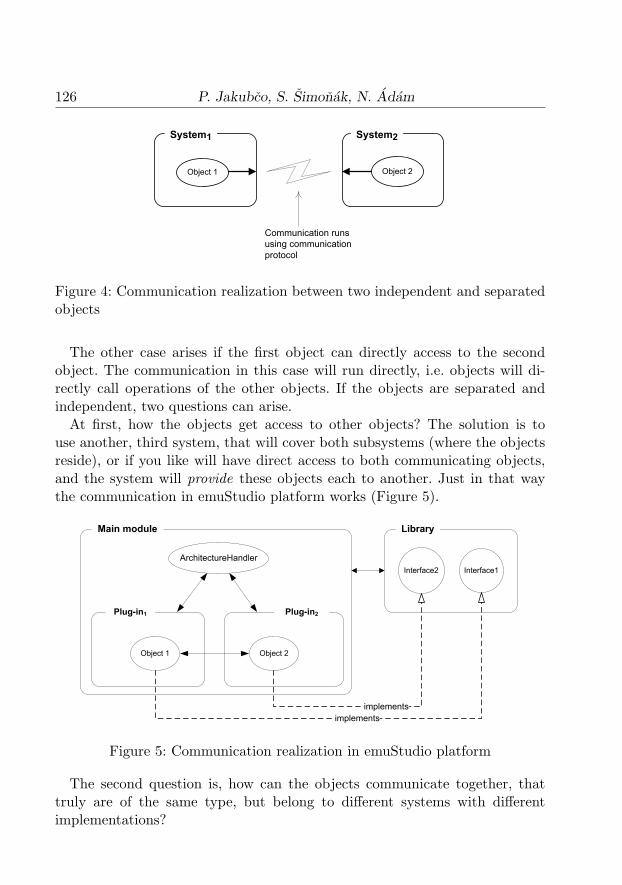
126 P. Jakubco, S. Simonak, N. Adam
Communication runs
using communication
protocol
Object 2Object 1
System1 System2
Figure 4: Communication realization between two independent and separatedobjects
The other case arises if the first object can directly access to the secondobject. The communication in this case will run directly, i.e. objects will di-rectly call operations of the other objects. If the objects are separated andindependent, two questions can arise.
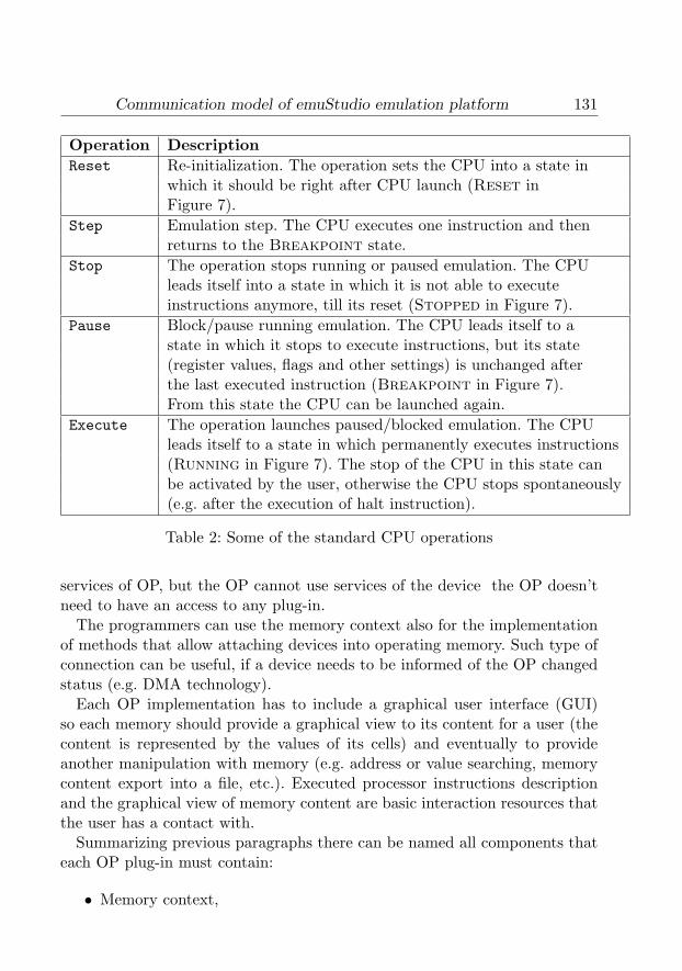
At first, how the objects get access to other objects? The solution is touse another, third system, that will cover both subsystems (where the objectsreside), or if you like will have direct access to both communicating objects,and the system will provide these objects each to another. Just in that waythe communication in emuStudio platform works (Figure 5).
ArchitectureHandler
Object 1 Object 2
Main module
Plug-in1 Plug-in2
Interface1Interface2
implements
implements
Library
Figure 5: Communication realization in emuStudio platform
The second question is, how can the objects communicate together, thattruly are of the same type, but belong to different systems with differentimplementations?

Communication model of emuStudio emulation platform 127
The solution is to create a standard model of operations that all the ob-jects of given type will implement and it will be well-known to all objects.This model has to unify both the syntax and semantics of communicationoperations.
The main module represents a system of higher level, covering subsystemsplug-ins. The objects of plug-ins the main module will get in virtual architec-ture instance creation process.
Communication operations are well-known both by the main module andby plug-ins. This is ensured by the fact that prototypes of the operationslies in external library, where the access is granted to both the main moduleand plug-ins. The operations are ordered according to the plug-in type intointerfaces (an interface is defined as a structure containing a list of operationswithout their implementation). Each plug-in type has its own set of interfacesthat corresponding plug-in has to implement.
4.1 External library structure
Figure 6 shows the structure of the external library, and contains all the pro-totypes (interfaces) for plug-ins.
Besides the packages and interfaces intended for the plug-ins to use, it con-tains a class called runtime.StaticDialogs, too. The class contains staticmethods that should disburden the plug-ins from common, fundamental andvery often used methods implementation.
4.2 Standard operations – Compiler
Every compiler generally consists of these parts:
• Lexical analyzer,• Syntactic analyzer (parser) that builds abstract syntactic tree,• Semantic analyzer that verifies types usage and other semantic informa-
tion,• Code generator that generates a machine code using abstract syntactic
tree.
Only some of these parts are important for interaction with the main mod-ule and plug-ins. Lexical and syntactic analyzer need to have the access tothe source code itself. Semantic analyzer can work with knowledge gainedfrom the phase of syntactic analysis (abstract syntactic tree), it means that

128 P. Jakubco, S. Simonak, N. Adam
plugins
runtime
memory device
StaticDialogs
+showErrorMessage(message:String):void
+showMessage(message:String):void
+getModelVersion():int
+getModelMinor():int
IMemory IMemoryContext IDevice IDeviceContext
ISettingsHandler IPlugin IContext
ILexer ICompiler ICPU ICPUContext
IDebugColumnIMessageReporterIToken
compiler cpu
Figure 6: Library structure
semantic analyzer won’t be in direct interaction with main module or otherplug-ins. Therefore it is possible to skip all considerations of assigning it intoa communication model.
Machine code generator can have an access to operating memory, too if theuser asks to redirect the compiler output into operating memory. On the otherhand, the main module needs to have an access to lexical analyzer, in orderto make possible to use syntax highlighting in source code editor. Finally, themain module needs to call the compile operation itself.

Communication model of emuStudio emulation platform 129
In Table 1 basic standard operations are described that are important fromthe communication point of view.
Operation DescriptionCompile Source code compilingGetLexer Gets an lexical analyzer objectGetStartAddress Gets absolute starting address of compiled program.
The address can be later used as starting address forthe program counter after the CPU Reset signal.
Table 1: Standard compiler operations
4.3 Standard CPU operations
Processor, or if you like the CPU, is a core of the architecture. It realizesthe execution of the whole emulation, because its main activity is instructionexecution. It also interacts with peripheral devices and with operating memory.Communication model does not limit the usage of the emulation technique forthe processor emulation.
The CPU plug-in in the emuStudio platform besides the emulation itself,it has to co-operate with the user by the interaction using debugger andstatus windows (however operations related to the interaction will not be de-scribed here). In the status window the CPU should show the values of itsregisters, flags, actual CPU’s running state and eventually other character-istics. The plug-in includes complete status window implementation so withdifferent CPU the content of the status window will change accordingly.
Generally each CPU plug-in consists of following parts:
• The processor emulation implementation,• Processor context that extends its functionality,• Instruction disassembler,• Status window GUI.
The CPU plug-in design demands the programmer to know the hardwarethat he is going to implement and to ”answer the questions correctly” whenthe interface methods implementation are considered.
The work-flow cycle of each processor plug-in for the emuStudio platformis shown in Figure 7. As it can be seen from the figure, the processor canbe found in one of four states. The Reset state is that state in which the

130 P. Jakubco, S. Simonak, N. Adam
processor re-initializes itself and immediately after finishing that it sets itselfto the Breakpoint state.
For the processor execution only the three states are meaningful:
• Breakpoint - the processor is temporally inactive (paused)• Running - the processor is running (executing instructions)• Stopped - the processor is stopped (waits for Reset signal)
RESET
RUNNING
BREAKPOINT
STOPPED
Start
End
End of emulation?
[pause]
[stop]
[run]
[stop]
[yes]
[no]
Figure 7: Processor work-flow cycle
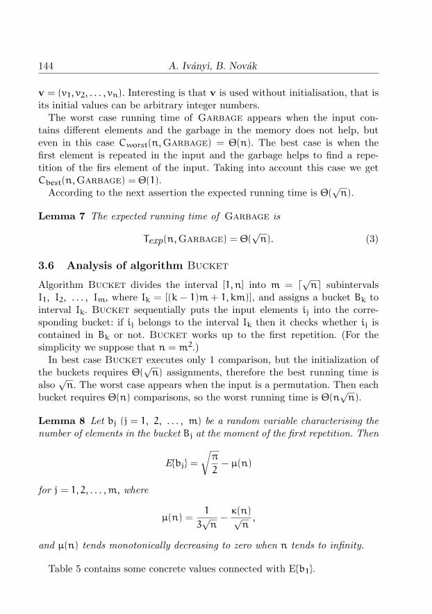
The Table 2 describes basic operations to control the processor execution inthe communication model. These operations tell how the CPU behavior can beinfluenced. However all of the operations are not supported in the real CPU’sworld and by contrast there definitely exist some CPU control operations thatare not covered by the communication model. But mostly such operations arenot common for all CPUs; therefore their support is optional within the scopeof CPU context.
4.4 Standard operations – Operating memory
Operating memory (OP) is not a computer component that directly affectsother computer components. It means that the memory is not “demanding”for services it is not acting like a communication initiator with the CPU, norwith the other devices (according to von Neumann conception). This fact iscovered by the communication model all connections with the OP are one-directional, and the OP is always plugged into the device (or into a processor),and not in the other way. It means that the device (or processor) can use
Communication model of emuStudio emulation platform 131
Operation DescriptionReset Re-initialization. The operation sets the CPU into a state in
which it should be right after CPU launch (Reset inFigure 7).
Step Emulation step. The CPU executes one instruction and thenreturns to the Breakpoint state.
Stop The operation stops running or paused emulation. The CPUleads itself into a state in which it is not able to executeinstructions anymore, till its reset (Stopped in Figure 7).
Pause Block/pause running emulation. The CPU leads itself to astate in which it stops to execute instructions, but its state(register values, flags and other settings) is unchanged afterthe last executed instruction (Breakpoint in Figure 7).From this state the CPU can be launched again.
Execute The operation launches paused/blocked emulation. The CPUleads itself to a state in which permanently executes instructions(Running in Figure 7). The stop of the CPU in this state canbe activated by the user, otherwise the CPU stops spontaneously(e.g. after the execution of halt instruction).
Table 2: Some of the standard CPU operations
services of OP, but the OP cannot use services of the device the OP doesn’tneed to have an access to any plug-in.
The programmers can use the memory context also for the implementationof methods that allow attaching devices into operating memory. Such type ofconnection can be useful, if a device needs to be informed of the OP changedstatus (e.g. DMA technology).
Each OP implementation has to include a graphical user interface (GUI)so each memory should provide a graphical view to its content for a user (thecontent is represented by the values of its cells) and eventually to provideanother manipulation with memory (e.g. address or value searching, memorycontent export into a file, etc.). Executed processor instructions descriptionand the graphical view of memory content are basic interaction resources thatthe user has a contact with.
Summarizing previous paragraphs there can be named all components thateach OP plug-in must contain:
• Memory context,

132 P. Jakubco, S. Simonak, N. Adam
• Implementation of main interface - the memory functionality itself,
• Graphical user interface (GUI).
Basic operations that have to be implemented in each operating memoryare described in Table 3.
Operation DescriptionRead Reading from operating memory - either one or more cells at
once starting from given address.Write Writing into operating memory - either one or more cells at
once starting from given address.ShowGUI The operation shows graphical user interface (GUI) of
memory content.
Table 3: Some of the operating memory standard operations
4.5 Standard operations - Peripheral devices
There are known input, output and input-output devices. Their category canbe identified easily according to a way how they are connected with other com-ponents of the configuration and to the direction of the connection (directionof data flow).
It is possible to implement virtual devices that communicate with real de-vices, but also fictive and abstract devices can be implemented. The devicecan interact with the user through its own graphical interface (GUI). Not alldevices have to have GUI, but on the other hand there are such devices thattheir input and/or output are realized using the user interaction (e.g. termi-nals, displays). The devices can communicate with CPU, OP and with otherdevices, too.
A single device can be connected multiple times with other components.For this reason the devices can have several contexts, with possible differentimplementations. For example a serial card can have several physical ports,into which it is possible to plug in various devices (into each port can beplugged a single device, and each port is represented by a single context).
Communication model solves the following problems:
• How to connect devices to each other,
• How to realize input/output.

Communication model of emuStudio emulation platform 133
The basic idea of interconnection of two devices in the meaning of implemen-tation is their contexts exchange with each other. All input/output operationsthat the devices will use for the communication resides in the context. In sucha way the bidirectional connection is realized. Each device contains an oper-ation intended for attaching of another device (op. attachDevice), that as aparameter takes the context of connecting device. This connection operationdoes not reside in the context, in order to ensure that the plug-ins couldn’tchange the structure of the virtual architecture. The connection job itself doesthe main module that performs the interconnection only in the virtual archi-tecture creation process.
The input and output operations (in and out) reside in the device context,because by calling them the communication is performed. Transferred datatype in these operations is not specified in the communication model, but it isdefined by the plug-ins. The java Objects are therefore transferred (they arereturned by the in method and the out method uses it as a parameter).
5 Conclusions
As far as we know, the emuStudio platform is the first attempt of the imple-mentation of both the universal and interactive emulation platform with theemulated components realized via plug-ins. In the present time the platformis used as a teaching support tool for chosen subjects at the Department ofComputers and Informatics, Faculty of Electrical Engineering and Informat-ics, Technical University of Kosice, Slovakia, in its still expanding form formore than two years.
The versatility and configurability allows creating plug-ins of various lev-els of quality and purpose - they can be intended for pedagogic or even forscientific purposes - e.g. the implementation of plug-ins that emulate the realhardware with the support of measurement of various characteristics, or asone of the phases of design of new hardware or for its testing, etc.
For ensuring the platform’s versatility it is important to stabilize the require-ments, to standardize components and mainly to design a way of communica-tion in the form of communication protocol, language or other mechanism.
The paper describes the mechanism of communication used in the emuStu-dio platform at the basic level. The communication mechanism still is not inits final form. Till the present time the 8-bit architectures (MITS Altair8800and its modification) and two abstract machines (Random Access Machine,BrainDuck - our own architecture) are implemented only.

134 P. Jakubco, S. Simonak, N. Adam
We believe that in the future the platform will be enhanced and the com-munication model finished and formally verified. There still is a free space forexpanding the platform by adding new emulated computer architectures.
References
[1] J. von Neumann, First Draft of a Report on the EDVAC, 1945. ⇒118
[2] N. Salmoria et al., MAME. The official site of the MAME developmentteam. ⇒118
[3] E. Freyre et al., Keeping emulation environments portable (KEEP). ⇒118
[4] P. Jakubco, S. Simonak, emuStudio – a plugin based emulation platform,J. Information, Control and Management Systems, 7, 1 (2009) 33–46. ⇒118
[5] M. Jelsina, Architectures of computer systems: principles, structuring or-ganisation, function (in Slovak), Elfa, Kosice, 2002, 567 p. ⇒118
[6] T. Kasai, Computational complexity of multitape Turing machines andrandom access machines, Publ. Res. Inst. Math. Sci., 13, 2 (1977) 469–496. ⇒118
[7] MITS, Inc., Altair 8080 Operators Manual , 1975. ⇒118
[8] S. Simonak, P. Jakubco, Software based CPU emulation, Acta Electrotech-nica et Informatica, 8, 4 (2008) 50–59. ⇒118, 124
[9] L. Vokorokos et al., Digital computer principles (in Slovak), Elfa, Kosice,2008, 322 p. ⇒118
Received: March 12, 2010 • Revised: June 25, 2010

Acta Univ. Sapientiae, Informatica, 2, 2 (2010) 135–153
Testing of sequences by simulation
Antal IvanyiEotvos Lorand University
Department of Computer AlgebraH-1117, Budapest, Hungary
Pazmany setany 1/Cemail: [email protected]
Balazs NovakEotvos Lorand University
Department of Computer AlgebraH-1117, Budapest, Hungary
Pazmany setany 1/Cemail: [email protected]
Abstract. Let ξ be a random integer vector, having uniform distribution
P{ξ = (i1, i2, . . . , in) = 1/nn} for 1 ≤ i1, i2, . . . , in ≤ n.
A realization (i1, i2, . . . , in) of ξ is called good, if its elements are dif-ferent. We present algorithms Linear, Backward, Forward, Tree,Garbage, Bucket which decide whether a given realization is good.We analyse the number of comparisons and running time of these algo-rithms using simulation gathering data on all possible inputs for smallvalues of n and generating random inputs for large values of n.
1 Introduction
Let ξ be a random integer vector, having uniform distribution
P{ξ = (i1, i2, . . . , in)} = 1/nn
for 1 ≤ i1, i2, . . . , in ≤ n.A realization (i1, i2, . . . , in) of ξ is called good, if its elements are different.
We present six algorithms which decide whether a given realization is good.This problem arises in connection with the design of agricultural [4, 5, 57, 72]
and industrial [34] experiments, with the testing of Latin [1, 9, 22, 23, 27, 32,
Computing Classification System 1998: G.2.2Mathematics Subject Classification 2010: 68M20Key words and phrases: random sequences, analysis of algorithms, Latin squares, sudokusquares
135

136 A. Ivanyi, B. Novak
53, 54, 63, 64] and sudoku [3, 4, 6, 12, 13, 14, 15, 16, 17, 20, 21, 22, 26, 29,30, 31, 41, 42, 44, 46, 47, 51, 55, 59, 61, 64, 66, 67, 68, 69, 70, 72, 74] squares,with genetic sequences and arrays [2, 7, 8, 18, 24, 28, 35, 36, 37, 38, 45, 48,49, 50, 56, 65, 71, 73, 75], with sociology [25], and also with the analysis of theperformance of computers with interleaved memory [11, 33, 39, 40, 41, 43, 52].
Section 2 contains the pseudocodes of the investigated algorithms. In Section3 the results of the simulation experiments and the basic theoretical resultsare presented. Section 4 contains the summary of the paper.
Further simulation results are contained in [62]. The proofs of the lemmasand theorems can be found in [43].
2 Pseudocodes of the algorithms
This section contains the pseudocodes of the investigated algorithms Linear,Backward, Forward, Tree, Garbage, and Bucket. The psudocode con-ventions described in the book [19] written by Cormen, Leiserson, Rivest, andStein are used.
The inputs of the following six algorithms are n (the length of the sequences) and s = (s1, s2, . . . , sn), a sequence of nonnegative integers with 0 ≤ si ≤ nfor 1 ≤ i ≤ n) in all cases. The output is always a logical variable g (its valueis True, if the input sequence is good, and False otherwise).
The working variables are usually the cycle variables i and j.
2.1 Definition of algorithm Linear
Linear writes zero into the elements of an n length vector v = (v1, v2,
. . . , vn), then investigates the elements of the realization and if v[si] > 0
(signalising a repetition), then stops, otherwise adds 1 to v[s[i]].
Linear(n, s)
01 g← True02 for i← 1 to n03 do v[i]← 0
04 for i← 1 to n05 do if v[s[i]] > 006 then g← False07 return g08 else v[s[i]]← v[s[i]] + 1
09 return g

Testing of sequences by simulation 137
2.2 Definition of algorithm Backward
Backward compares the second (i2), third (i3), . . . , last (in) element of therealization s with the previous elements until the first collision or until thelast pair of elements.
Backward(n, s)
01 g← True02 for i← 2 to n03 do for j← i− 1 downto 104 do if s[i] = s[j]
05 then g← False06 return g07 return g
2.3 Definition of algorithm Forward
Forward compares the first (s1), second (s2), . . . , last but one (sn−1) elementof the realization with the following elements until the first collision or untilthe last pair of elements.
Forward(n, s)
01 g← True02 for i← 1 to n− 1
03 do for j← i+ 1 to n04 do if s[i] = s[j]
05 then g← False06 return g07 return g
2.4 Definition of algorithm Tree
Tree builds a random search tree from the elements of the realization andfinishes the construction of the tree if it finds the following element of therealization in the tree (then the realization is not good) or it tested the lastelement too without a collision (then the realization is good).
Tree(n, s)
01 g← True02 let s[1] be the root of a tree03 for i← 2 to n

138 A. Ivanyi, B. Novak
04 if [s[i] is in the tree05 then g← False06 return07 else insert s[i] in the tree08 return g
2.5 Definition of algorithm Garbage
This algorithm is similar to Linear, but it works without the setting zerosinto the elements of a vector requiring linear amount of time.
Beside the cycle variable i Garbage uses as working variable also a vectorv = (v1, v2, . . . , vn). Interesting is that v is used without initialisation, that isits initial values can be arbitrary integer numbers.
The algorithm Garbage was proposed by Gabor Monostori [58].
Garbage(n, s)
01 g← True02 for i← 1 to n03 do if v[s[i]] < i and s[v[s[i]]] = s[i]
04 then g← False05 return g06 else v[s[i]]← i
07 return g
2.6 Definition of algorithm Bucket
Bucket handles the array Q[1 : m, 1 : m] (where m = d√ne and puts the
element si into the rth row of Q, where r = dsi/me and it tests using linearsearch whether sj appeared earlier in the corresponding row. The elements ofthe vector c = (c1, c2, . . . , cm) are counters, where cj (1 ≤ j ≤ m) shows thenumber of elements of the ith row.
For the simplicity we suppose that n is a square.
Bucket(n, s)
01 g← True02 m← √n03 for j← 1 to m04 do c[j]← 1
05 for i← 1 to n06 do r← ds[i]/mem

Testing of sequences by simulation 139
07 for j← 1 to c[r] − 1
08 do if s[i] = Q[r, j]
09 then g← False10 return g11 else Q[r, c[r]]← s[i]
12 c[r]← c[r] + 1
13 return g
3 Analysis of the algorithms
3.1 Analysis of algorithm Linear
The first algorithm is Linear. It writes zero into the elements of an n lengthvector v = (v1, v2, . . . , vn), then investigates the elements of the realiza-tion sequentially and if ij = k, then adds 1 to vk and tests whether vk > 0
signalizing a repetition.In best case Linear executes only two comparisons, but the initialization of
the vector v requires Θ(n) assignments. It is called Linear, since its runningtime is Θ(n) in best, worst and so also in expected case.
Theorem 1 The expected number Cexp(n,Linear) = CL of comparisons ofLinear is
CL = 1−n!
nn+
n∑k=1
n!k2
(n− k)!nk+1
=
√πn
2+2
3+ κ(n) −
n!
nn,
where
κ(n) =1
3−
√πn
2+
n∑k=1
n!k
(n− k)!nk+1
tends monotonically decreasing to zero when n tends to infinity. n!/nn alsotends monotonically decreasing to zero, but their difference δ(n) = κ(n) −
n!/nn is increasing for 1 ≤ n ≤ 8 and is decreasing for n ≥ 8.
Theorem 2 The expected running time Texp(n,Linear) = TL of Linear is
TL = n+√2πn+
7
3+ 2δ(n),

140 A. Ivanyi, B. Novak
n CL√πn/2+ 2/3 n!/nn κ(n) δ(n)
1 1.000000 1.919981 1.000000 0.080019 −0.919981
2 2.000000 2.439121 0.500000 0.060879 −0.439121
3 2.666667 2.837470 0.222222 0.051418 −0.170804
4 3.125000 3.173295 0.093750 0.045455 −0.048295
5 3.472000 3.469162 0.038400 0.041238 +0.002838
6 3.759259 3.736647 0.015432 0.038045 +0.022612
7 4.012019 3.982624 0.006120 0.035515 +0.029395
8 4.242615 4.211574 0.002403 0.033444 +0.031040
9 4.457379 4.426609 0.000937 0.031707 +0.030770
10 4.659853 4.629994 0.000363 0.030222 +0.029859
Table 1: Values of CL,√πn/2 + 2/3, n!/nn, κ(n), and δ(n) = κ(n) − n!/nn
for n = 1, 2, . . . , 10
whereδ(n) = κ(n) −
n!
nn
tends to zero when n tends to infinity, further
δ(n+ 1) > δ(n) for 1 ≤ n ≤ 7 and δ(n+ 1) < δ(n) for n ≥ 8.
Table 1 shows some concrete values connected with algorithm Linear.
3.2 Analysis of algorithm Backward
The second algorithm is Backward. This algorithm is a naive comparison-based one. Backward compares the second (i2), third (i3), . . . , last (in)
element of the realization with the previous elements until the first repetitionor until the last pair of elements.
The running time of Backward is constant in the best case, but it isquadratic in the worst case.
Theorem 3 The expected number Cexp(n,Backward) = CB of comparisonsof the algorithm Backward is
CB = n+
√πn
8+2
3− α(n),
where α(n) = κ(n)/2+ (n!/nn)((n+ 1)/2) monotonically decreasing tends tozero when n tends to ∞.

Testing of sequences by simulation 141
Table 2 shows some concrete values characterizing algorithm Backward.
n CB n−√πn/8+ 2/3 (n!/nn)((n+ 1)/2) κ(n) α(n)
1 0.000000 1.040010 1.000000 0.080019 1.040010
2 1.000000 1.780440 0.750000 0.060879 0.780440
3 2.111111 2.581265 0.444444 0.051418 0.470154
4 3.156250 3.413353 0.234375 0.045455 0.257103
5 4.129600 4.265419 0.115200 0.041238 0.135819
6 5.058642 5.131677 0.054012 0.038045 0, 073035
7 5.966451 6.008688 0.024480 0.035515 0.042237
8 6.866676 6.894213 0.010815 0.033444 0.027536
9 7.766159 7.786695 0.004683 0.031707 0.020537
10 8.667896 8.685003 0.001996 0.030222 0.017107
Table 2: Values of CB, n−√πn/8+2/3, (n!/nn)((n+1)/2), κ(n), and α(n) =
κ(n)/2+ (n!/nn)((n+ 1)/2) for n = 1, 2, . . . , 10
The next assertion gives the expected running time of algorithm Back-ward.
Theorem 4 The expected running time Texp(n,Backward) = TB of the al-gorithm Backward is
TB = n+
√πn
8+4
3− α(n),
where α(n) = κ(n)/2+ (n!/nn)((n+ 1)/2) monotonically decreasing tends tozero when n tends to ∞.
3.3 Analysis of algorithm Forward
Forward compares the first (s1), second (s2), . . . , last but one (sn−1) elementof the realization with the next elements until the first collision or until thelast pair of elements.
Taking into account the number of the necessary comparisons in line 04 ofForward, we get Cbest(n,Forward) = 1 = Θ(1), and Cworst(n,Forward) =
B(n, 2) = Θ(n2).The next assertion gives the expected running time.

142 A. Ivanyi, B. Novak
Theorem 5 The expected running time Texp(n,Forward) = TF of the algo-rithm Forward is
TF = n+Θ(√n). (1)
Although the basic characteristics of Forward and Backward are iden-tical, as Table 3 shows, there is a small difference in the expected behaviour.
n number of sequences number of good sequences CF CW2 4 2 1.000000 1.000000
3 27 6 2.111111 2.111111
4 256 24 3.203125 3.156250
5 3 125 120 4.264000 4.126960
6 46 656 720 5.342341 5.058642
7 823 543 5 040 6.326760 5.966451
8 16 777 216 40 320 7.342926 6.866676
9 387 420 489 362 880 8.354165 7.766159
Table 3: Values of n, the number of possible input sequences, number of goodsequences, expected number of comparisons of Forward (CF) and expectednumber of comparisons of Backward (CW) for n = 2, 3, . . . , 9
3.4 Analysis of algorithm Tree
Tree builds a random search tree from the elements of the realization andfinishes the construction of the tree if it finds the following element of therealization in the tree (then the realization is not good) or it tested the lastelement too without a collision (then the realization is good).
The worst case running time of Tree appears when the input containsdifferent elements in increasing or decreasing order. Then the result is Θ(n2).The best case is when the first two elements of s are equal, so Cbest(n,Tree) =
1 = Θ(1).Using the known fact that the expected height of a random search tree is
Θ(lgn) we can get that the order of the expected running time is√n logn.
Theorem 6 The expected running time TT of Tree is
TT = Θ(√n lgn). (2)

Testing of sequences by simulation 143
n number of good inputs number of comparisons number of assignments1 100 000.000000 0.000000 1.000000
2 49 946.000000 1.000000 1.499460
3 22 243.000000 2.038960 1.889900
4 9 396.000000 2.921710 2.219390
5 3 723.000000 3.682710 2.511409
6 1 569.000000 4.352690 2.773160
7 620.000000 4.985280 3.021820
8 251.000000 5.590900 3.252989
9 104 6.148550 3.459510
10 33 6.704350 3.663749
11 17 7.271570 3.860450
12 3 7.779950 4.039530
13 3 8.314370 4.214370
14 0 8.824660 4.384480
15 2 9.302720 4.537880
16 0 9.840690 4.716760
17 0 10.287560 4.853530
18 0 10.719770 4.989370
19 0 11.242740 5.147560
20 0 11.689660 5.279180
Table 4: Values of n, number of good inputs, number of comparisons, numberof assignments of Tree for n = 1, 2, . . . , 10
Table 4 shows some results of the simulation experiments (the number ofrandom input sequences is 100 000 in all cases).
Using the method of the smallest squares to find the parameters of theformula a
√n log2 n we received the following approximation formula for the
expected number of comparisons:
Cexp(n,Tree) = 1.245754√n log2 n− 0.273588.
3.5 Analysis of algorithm Garbage
This algorithm is similar to Linear, but it works without the setting zerosinto the elements of a vector requiring linear amount of time.
Beside the cycle variable i Garbage uses as working variable also a vector
144 A. Ivanyi, B. Novak
v = (v1, v2, . . . , vn). Interesting is that v is used without initialisation, that isits initial values can be arbitrary integer numbers.
The worst case running time of Garbage appears when the input con-tains different elements and the garbage in the memory does not help, buteven in this case Cworst(n,Garbage) = Θ(n). The best case is when thefirst element is repeated in the input and the garbage helps to find a repe-tition of the firs element of the input. Taking into account this case we getCbest(n,Garbage) = Θ(1).
According to the next assertion the expected running time is Θ(√n).
Lemma 7 The expected running time of Garbage is
Texp(n,Garbage) = Θ(√n). (3)
3.6 Analysis of algorithm Bucket
Algorithm Bucket divides the interval [1, n] into m = d√ne subintervals
I1, I2, . . . , Im, where Ik = [(k − 1)m + 1, km)], and assigns a bucket Bk tointerval Ik. Bucket sequentially puts the input elements ij into the corre-sponding bucket: if ij belongs to the interval Ik then it checks whether ij iscontained in Bk or not. Bucket works up to the first repetition. (For thesimplicity we suppose that n = m2.)
In best case Bucket executes only 1 comparison, but the initialization ofthe buckets requires Θ(
√n) assignments, therefore the best running time is
also√n. The worst case appears when the input is a permutation. Then each
bucket requires Θ(n) comparisons, so the worst running time is Θ(n√n).
Lemma 8 Let bj (j = 1, 2, . . . , m) be a random variable characterising thenumber of elements in the bucket Bj at the moment of the first repetition. Then
E{bj} =
√π
2− µ(n)
for j = 1, 2, . . . ,m, where
µ(n) =1
3√n
−κ(n)√n,
and µ(n) tends monotonically decreasing to zero when n tends to infinity.
Table 5 contains some concrete values connected with E{b1}.

Testing of sequences by simulation 145
n E{b1}√π/2 1/(3
√n) κ(n)/
√n µ(n)
1 1.000000 1.253314 0.333333 0.080019 0.2533142 1.060660 1.253314 0.235702 0.043048 0.1926543 1.090055 1.253314 0.192450 0.029686 0.1627644 1.109375 1.253314 0.166667 0.022727 0.1439405 1.122685 1.253314 0.149071 0.018442 0.1306296 1.132763 1.253314 0.136083 0.015532 0.1205517 1.147287 1.253314 0.125988 0.013423 0.1125658 1.147287 1.253314 0.117851 0.011824 0.1060279 1.152772 1.253314 0.111111 0.010569 0.10054210 1.157462 1.253314 0.105409 0.009557 0.095852
Table 5: Values of E{b1},√π/2, 1/(3
√n), κ(n)/
√n, and µ(n) = 1/(3
√n) −
κ(n)/√n of Bucket for n = 1, 2, . . . , 10
Lemma 9 Let fn be a random variable characterising the number of compar-isons executed in connection with the first repeated element. Then
E{fn} = 1+
√π
8− η(n),
where
η(n) =13 +
√π8 −
κ(n)2√
n+ 2,
and η(n) tends monotonically decreasing to zero when n tends to infinity.
Theorem 10 The expected number Cexp(n,Bucket) = CB of comparisonsof algorithm Bucket in 1 bucket is
CB =√n+
1
3−
√π
8+ ρ(n),
where
ρ(n) =5/6−
√9π/8− 3κ(n)/2√n+ 1
tends to zero when n and tends to infinity.

146 A. Ivanyi, B. Novak
Index and Algorithm Cbest(n) Cworst(n) Cexp(n)
1. Linear Θ(1) Θ(n) Θ(√n)
2. Backward Θ(1) Θ(n2) Θ(n)
3. Forward Θ(1) Θ(n2) Θ(n)
4. Tree Θ(1) Θ(n2) Θ(√n lgn)
5. Garbage Θ(1) Θ(n) Θ(√n)
6. Bucket Θ(√n) Θ(n
√n) Θ(
√n)
Table 6: The number of necessary comparisons of the investigated algorithmsin best, worst and expected cases
Theorem 11 The expected running time TB(n,Bucket) = TB of Bucket is
TB =
(3+ 3
√π
2
)√n+
√25π
8+ φ(n),
where
φ(n) = 3κ(n) − ρ(n) − 3η(n) −n!
nn−3√π/8− 1/3− 3κ(n)/2√
n+ 1
and φ(n) tends to zero when n tends to infinity.
It is worth to remark that simulation experiments of B. Novak [62] showthat the expected running time of Garbage is a few percent better, then theexpected running time of Bucket.
4 Summary
Table 6 contains the number of necessary comparisons in best, worst andexpected cases for all investigated algorithms.Table 7 contains the running time in best, worst and expected cases for allinvestigated algorithms.
Acknowledgements. The authors thank Tamas F. Mori [60] for provingLemma 8 and 9 and Peter Burcsi [10] for useful information on references,both are teachers of Eotvos Lorand University.
The European Union and the European Social Fund have provided finan-cial support to the project under the grant agreement no. TAMOP 4.2.1/B-09/1/KMR-2010-0003.

Testing of sequences by simulation 147
Index and Algorithm Tbest(n) Tworst(n) Texp(n)
1. Linear Θ(n) Θ(n) n+Θ(√n)
2. Backward Θ(1) Θ(n2) Θ(n)
3. Forward Θ(1) Θ(n2) Θ(n)
5. Tree Θ(1) Θ(n2) Θ(√n lgn)
6. Garbage Θ(1) Θ(n) Θ(√n)
7. Bucket Θ(√n) Θ(n
√n) Θ(
√n)
Table 7: The running times of the investigated algorithms in best, worst andexpected cases
References
[1] P. Adams, D. Bryant, M. Buchanan, Completing partial Latin squareswith two filled rows and two filled columns, Electron. J. Combin. 15, 1(2008), Research paper 56, 26 p. ⇒136
[2] M.-C. Anisiu, A. Ivanyi, Two-dimensional arrays with maximal complex-ity, Pure Math. Appl. (PU.M.A.) 17, 3–4 (2006) 197–204. ⇒136
[3] C. Arcos, G. Brookfield, M. Krebs, Mini-sudokus and groups, Math. Mag.83, 2 (2010) 111–122. ⇒136
[4] R. A. Bailey, R. Cameron, P. J. Connelly, Sudoku, gerechte designs, reso-lutions, affine space, spreads, reguli, and Hamming codes, American Math.Monthly 115, 5 (2008) 383–404. ⇒135, 136
[5] W. U. Behrens, Feldversuchsanordnungen mit verbessertem Ausgleichder Bodenunterschiede, Zeitschrift fur Landwirtschaftliches Versuchs- undUntersuchungswesen, 2 (1956) 176–193. ⇒135
[6] D. Berthier, Unbiased statistics of a constraint satisfaction problem –a controlled-bias generator, in: S. Tarek et al. (eds.), Innovations incomputing sciences and software engineering, Proc. Second InternationalConference on Systems, Computing Sciences and Software Engineering(SCSS’2009, December 4–12, 2009, Dordrecht). Springer, Berlin, 2010.pp. 91–97. ⇒136
[7] S. Brett, G. Hurlbert, B. Jackson, Preface [Generalisations of de Bruijncycles and Gray codes], Discrete Math., 309, 17 (2009) 5255–5258. ⇒136

148 A. Ivanyi, B. Novak
[8] A. A. Bruen, R. A. Mollin, Cryptography and shift registers, Open Math.J., 2 (2009) 16–21. ⇒136
[9] H. L. Buchanan, M. N. Ferencak, On completing Latin squares, J. Com-bin. Math. Combin. Comput., 34 (2000) 129–132. ⇒136
[10] P. Burcsi, Personal communication. Budapest, March 2009. ⇒146
[11] G. J. Burnett, E. G. Coffman, Jr., Combinatorial problem related tointerleaved memory systems, J. ACM, 20, 1 (1973) 39–45. ⇒136
[12] P. J. Cameron, Sudoku – an alternative history, Talk to the Archimedeans,Queen Mary University of London, February 2007. ⇒136
[13] A. Carlos, G. Brookfield, M. Krebs, Mini-sudokus and groups, Math.Mag., 83, 2 (2010) 111–122. ⇒136
[14] J. Carmichael, K. Schloeman, M. B. Ward, Cosets and Cayley-sudokutables, Math. Mag., 83, 2 (2010) 130–139. ⇒136
[15] Ch.-Ch. Chang, P.-Y. Lin, Z.-H. Wang, M.-Ch. Li, A sudoku-based secretimage sharing scheme with reversibility, J. Commun., 5, 1 (2010) 5–12.⇒136
[16] Z. Chen, Heuristic reasoning on graph and game complexity of sudoku,ARXIV.org, 2010. 6 p. ⇒136
[17] Y.-F. Chien, W.-K. Hon, Cryptographic and physical zero-knowledgeproof: From sudoku to nonogram, in: P. Boldi (ed.), Fun with Algorithms,(5th International Conference, FUN 2010, Ischia, Italy, June 2–4, 2010.)Springer, Berlin, 2010, Lecture Notes in Comput. Sci., 6099 (2010) 102–112. ⇒136
[18] J. Cooper, C. Heitsch, The discrepancy of the lex-least de Bruijn sequence,Discrete Math., 310, 6–7 (2010), 1152–1159. ⇒136
[19] T. H. Cormen, C. E. Leiserson, R. L. Rivest, C. Stein, Introduction toAlgorithms, Third edition. The MIT Press, Cambridge, 2009. ⇒136
[20] J. F. Crook, A pencil-and-paper algorithm for solving sudoku puzzles,Notices Amer. Math. Soc., 56 (2009) 460–468. ⇒136
[21] G. Dahl, Permutation matrices related to sudoku, Linear Algebra Appl.,430 (2009), 2457–2463. ⇒136

Testing of sequences by simulation 149
[22] J. Denes, A. D. Keedwell, Latin squares. New developments in the theoryand applications, North-Holland, Amsterdam, 1991. ⇒136
[23] T. Easton, R. G. Parker, On completing Latin squares, Discrete Appl.Math., 113, 2–3 (2001) 167–181. ⇒136
[24] C. H. Elzinga, S. Rahmann, H. Wung, Algorithms for subsequence com-binatorics, Theor. Comput. Sci., 409, 3 (2008) 394–404. ⇒136
[25] C. H. Elzinga, Complexity of categorial time series, Sociological Methods& Research, 38, 3 (2010) 463–481. ⇒136
[26] M. Erickson, Pearls of discrete mathematics, Discrete Mathematics andits Applications, CRC Press, Boca Raton, FL, 2010. ⇒136
[27] R. Euler, On the completability of incomplete Latin squares, EuropeanJ. Combin. 31 (2010) 535–552. ⇒136
[28] S. Ferenczi, Z. Kasa, Complexity for finite factors of infinite sequences,Theoret. Comput. Sci. 218, 1 (1999) 177–195. ⇒136
[29] R. Fontana, F. Rapallo, M. P. Rogantin, Indicator function and sudokudesigns, in: P. Gibilisco, E. Ricco-magno, M. P. Rogantin, H. P. Wynn(eds.) Algebraic and Geometric Methods in Statistics, pp. 203–224. Cam-bridge University Press, Cambridge, 2010. ⇒136
[30] R. Fontana, F. Rapallo, M. P. Rogantin, Markov bases for sudoku grids.Rapporto interno N. 4, marzo 2010, Politecnico di Torino. ⇒136
[31] A. F. Gabor, G. J. Woeginger, How *not* to solve a Sudoku. OperationResearch Letters, 38, 6 (2010) 582–584. ⇒136
[32] I. Hajirasouliha, H. Jowhari, R. Kumar, R. Sundaram, On completingLatin squares, Lecture Notes in Comput. Sci., 4393 (2007), 524–535.Springer, Berlin, 2007. ⇒136
[33] H. Hellerman, Digital computer system principles. Mc Graw Hill, NewYork, 1967. ⇒136
[34] A. Heppes, P. Revesz, A new generalization of the concept of latin squaresand orthogonal latin squares and its application to the design of exper-iments (in Hungarian), Magyar Tud. Akad. Mat. Int. Kozl., 1 (1956)379–390. ⇒135

150 A. Ivanyi, B. Novak
[35] M. Horvath, A. Ivanyi, Growing perfect cubes, Discrete Math., 308, 19(2008) 4378–4388. ⇒136
[36] A. Ivanyi, On the d-complexity of words, Ann. Univ. Sci. Budapest. Sect.Comput. 8 (1987) 69–90 (1988). ⇒136
[37] A. Ivanyi, Construction of infinite de Bruijn arrays, Discrete Appl. Math.22, 3 (1988/89), 289–293. ⇒136
[38] A. Ivanyi, Construction of three-dimensional perfect matrices, (TwelfthBritish Combinatorial Conference, Norwich, 1989). Ars Combin. 29C(1990) 33–40. ⇒136
[39] A. Ivanyi, I. Katai, Estimates for speed of computers with interleavedmemory systems, Ann. Univ. Sci. Budapest. Sect. Math., 19 (1976) 159–164. ⇒136
[40] A. Ivanyi, I. Katai, Processing of random sequences with priority, ActaCybern. 4, 1 (1978/79) 85–101. ⇒136
[41] A. Ivanyi, I. Katai, Quick testing of random variables, Proc. ICAI’2010(Eger, January 27–30, 2010). To appear. ⇒136
[42] A. Ivanyi, I. Katai, Testing of uniformly distributed vectors, in: AbstractsJanos Bolyai Memorial Conference, (Budapest, August 28–30, 2010), p.47. ⇒136
[43] A. Ivanyi, I. Katai, Testing of random matrices, Ann. Univ. Sci. Budapest.Sect. Comput. (submitted). ⇒136
[44] A. Ivanyi, B. Novak, Testing of random sequences by simulation, in: Ab-stracts 8th MACS (Komarno, July 14–17, 2010). ⇒136
[45] A. Ivanyi, Z. Toth, Existence of de Bruijn words, Second Conferenceon Automata, Languages and Programming Systems (Salgotarjan, 1988),165–172, DM, 88-4, Karl Marx Univ. Econom., Budapest, 1988. ⇒136
[46] I. Kanaana, B. Ravikumar, Row-filled completion problem for sudoku,Util. Math. 81 (2010) 65–84. ⇒136
[47] Z. Karimi-Dehkordi, K. Zamanifar, A. Baraani-Dastjerdi, N. Ghasem-Aghaee, Sudoku using parallel simulated annealing, in: Y. Tan et al.
Testing of sequences by simulation 151
(eds.), Advances in Swarm Intelligence (Proc. First International Con-ference, ICSI 2010, Beijing, China, June 12–15, 2010, Part II. LectureNotes in Comput. Sci., 6146 (2010) 461–467, Springer, Berlin, 2010. ⇒136
[48] Z. Kasa, Computing the d-complexity of words by Fibonacci-like se-quences, Studia Univ. Babes-Bolyai Math. 35, 3 (1990) 49–53. ⇒136
[49] Z. Kasa, Pure Math. Appl. On the d-complexity of strings, (PU.M.A.) 9,1–2 (1998) 119–128. ⇒136
[50] Z. Kasa, Super-d-complexity of finite words, Proc. 8th Joint Conferenceon Mathematics and Computer Science, (Komarno, Slovakia, July 14–17),2010, To appear. ⇒136
[51] A. D. Keedwell, Constructions of complete sets of orthogonal diagonalsudoku squares, Australas. J. Combin. 47 (2010) 227–238. ⇒136
[52] D. E. Knuth, The art of computer programming, Vol. 1. Fundamentalalgorithms (third edition). Addison–Wesley, Reading, MA, 1997. ⇒136
[53] J. S. Kuhl, T. Denley, On a generalization of the Evans conjecture, Dis-crete Math. 308, 20 (2008), 4763–4767. ⇒136
[54] S. R. Kumar S., A. Russell, R. Sundaram, Approximating Latin squareextensions, Algorithmica 24, 2 (1999) 128–138. ⇒136
[55] L. Lorch, Mutually orthogonal families of linear sudoku solutions, J. Aust.Math. Soc., 87, 3 (2009) 409–420. ⇒136
[56] M. Matamala, F. Moreno, Minimum Eulerian circuits and minimum deBruijn sequences, Discrete Math., 309, 17 (2009) 5298–5304. ⇒136
[57] H.-D. Mo, R.-G. Xu, Sudoku square – a new design in field, Acta Agro-nomica Sinica, 34, 9 (2008) 1489–1493. ⇒135
[58] G. Monostori, Personal communication, Budapest, May 2010. ⇒138
[59] T. K. Moon, J. H. Gunther, J. J. Kupin, Sinkhorn solves sudoku,IEEETrans. Inform. Theory , 55, 4 (2009) 1741–1746. ⇒136
[60] T. Mori, Personal communication, Budapest, April 2010. ⇒146

152 A. Ivanyi, B. Novak
[61] P. K. Newton, S. A. deSalvo, The Shannon entropy of sudoku matrices,Proc. R. Soc. Lond. Ser. A, Math. Phys. Eng. Sci. 466 (2010) 1957-1975.⇒136
[62] B. Novak, Analysis of sudoku algorithms (in Hungarian), MSc thesis,Eotvos Lorand University, Fac. of Informatics, Budapest, 2010. ⇒ 136,146
[63] L.-D. Ohman, A note on completing Latin squares, Australas. J. Combin.,45 (2009) 117–123. ⇒136
[64] R. M. Pedersen, T. L. Vis, Sets of mutually orthogonal sudoku Latinsquares. College Math. J., 40, 3 (2009) 174–180. ⇒136
[65] R. Penne, A note on certain de Bruijn sequences with forbidden subse-quences, Discrete Math., 310, 4 (2010) 966–969. ⇒136
[66] J. S. Provan, Sudoku: strategy versus structure, Amer. Math. Monthly ,116, 8 (2009), 702–707. ⇒136
[67] T. Sander, Sudoku graphs are integral, Electron. J. Combin., 16, 1 (2009),Note 25, 7 p. ⇒136
[68] Y. Sato, H. Inoue, Genetic operations to solve sudoku puzzles, Proc.12th Annual Conference on Genetic and Evolutionary ComputationGECCO’10, July 7–11, 2010, Portland, OR, pp. 2111–21012. ⇒136
[69] M. J. Soottile, T. G. Mattson, C. E. Rasmussen, Introduction to concur-rency in programming languages, Chapman & Hall/CRC ComputationalScience Series. CRC Press, Boca Raton, FL, 2010. ⇒136
[70] D. Thom, SUDOKU ist NP-vollstandig, PhD Dissertation, Stuttgart,2007. ⇒136
[71] O. G. Troyanskaya, O. Arbell, Y. Koren, G. M. Landau, A. Bolshoy, Se-quence complexity profiles of prokaryotic genomic sequences: A fast algo-rithm for calculating linguistic complexity, Bioinformatics, 18, 5 (2002)679–688. ⇒136
[72] E. R. Vaughan, The complexity of constructing gerechte designs, Electron.J. Combin., 16, 1 (2009), paper R15, 8 p. ⇒135, 136
[73] X. Xu, Y. Cao, J.-M. Xu, Y. Wu, Feedback numbers of de Bruijn digraphs,Comput. Math. Appl., 59, 4 (2010), 716–723. ⇒136

Testing of sequences by simulation 153
[74] C. Xu, W. Xu, The model and algorithm to estimate the difficulty levelsof sudoku puzzles, J. Math. Res. 11, 2 (2009), 43–46. ⇒136
[75] W. Zhang, S. Liu, H. Huang, An efficient implementation algorithm forgenerating de Bruijn sequences, Computer Standards & Interfaces, 31, 6(2009) 1190–1191. ⇒136
Received: August 20, 2010 • Revised: October 15, 2010

Acta Univ. Sapientiae, Informatica, 2, 2 (2010) 154–167
Testing by C++ template metaprograms
Norbert PatakiDept. of Programming Languages and CompilersFaculty of Informatics, Eotvos Lorand University
Pazmany Peter setany 1/C H-1117 Budapest,Hungary
email: [email protected]
Abstract. Testing is one of the most indispensable tasks in software en-gineering. The role of testing in software development has grown signifi-cantly because testing is able to reveal defects in the code in an early stageof development. Many unit test frameworks compatible with C/C++code exist, but a standard one is missing. Unfortunately, many unsolvedproblems can be mentioned with the existing methods, for example usu-ally external tools are necessary for testing C++ programs.
In this paper we present a new approach for testing C++ programs.Our solution is based on C++ template metaprogramming facilities, so itcan work with the standard-compliant compilers. The metaprogrammingapproach ensures that the overhead of testing is minimal at runtime. Thisapproach also supports that the specification language can be customizedamong other advantages. Nevertheless, the only necessary tool is thecompiler itself.
1 Introduction
Testing is the most important method to check programs’ correct behaviour.Testing can reveal many problems within the code in development phase. Test-ing is cruicial from the view of software quality [5]. Many purposes of testingcan be, for instance, quality assurance, verification and validation, or reliabilityestimation. Nonetheless, testing is potentially endless. It can never completely
Computing Classification System 1998: D.2.5Mathematics Subject Classification 2010: 62N03Key words and phrases: testing, C++, template metaprogramming
154

Testing by C++ template metaprograms 155
identify all the defects within the software. The main task is is to deliverfaultless software [20].
Correctness testing and reliability testing are two major areas of testing.However, many different testing levels are used. In this paper we deal withunit tests that is about correctness. The goal of unit testing is to isolate eachpart of the program and to show that the individual parts are correct. A unittest provides a strict, written contract that the piece of code must satisfy.As a result, it affords several benefits. Unit tests find problems early in thedevelopment phase. Unfortunately, most frameworks need external tools [10].
A testing framework is proposed in [3, 4] which is based on the C++0x – theC++ forthcoming standard. The framework takes advantage of concepts andaxioms. These constructs support the generic programming in C++ as theyenable to write type constraints in template parameters. By now, these con-structs are removed from the draft of the next standard. Metaprogram testingframework has already been developed [16] too, but it deals with metaprogams,it is just the opposite of our approach.
C++ template metaprogramming is an emerging paradigm which enablesto execute algorithms when ordinary C++ programs are compiled. The styleof C++ template metaprograms is very similar to the functional program-ming paradigm. Metaprograms have many advantages that we can harness.Metalevel often subserves the validation [8].
Template metaprograms run at compilation-time, whereupon the overheadat runtime is minimal. Metaprograms’ “input” is the runtime C++ programitself, therefore metaprograms are able to retrieve information about the host-ing program. This way we can check many properties about the programsduring compilation [12, 14, 21, 22].
Another important feature of template metaprograms is the opportunity ofdomain-specific languages. These special purpose languages are integrated intoC++ by template metaprograms [7, 9]. Libraries can be found that support thedevelopment of domain-specific languages [11]. New languages can be figuredout to write C++ template metaprograms [18]. Special specification languagescan be used for testing C++ programs without external tools.
In this paper we present a new approach to test C++ code. Our frameworkis based on the metaprogramming facility of C++. We argue for testing bymeta-level because of numerous reasons.
The rest of this paper is organized as follows. In Section 2 C++ templatemetaprograms are detailed. In Section 3 we present the basic ideas behind ourapproach, after that in Section 4 we analyze the advantages and disadvantagesof our framework. Finally, the future work is detailed in Section 5.

156 N. Pataki
2 C++ template metaprogramming
The template facility of C++ allows writing algorithms and data structuresparametrized by types. This abstraction is useful for designing general algo-rithms like finding an element in a list. The operations of lists of integers,characters or even user defined classes are essentially the same. The only dif-ference between them is the stored type. With templates we can parametrizethese list operations by type, thus, we have to write the abstract algorithmonly once. The compiler will generate the integer, double, character or userdefined class version of the list from it. See the example below:
template<typename T>struct list{
void insert( const T& t );// ...
};
int main(){
list<int> l; //instantiation for intlist<double> d; // and for doublel.insert( 42 ); // usaged.insert( 3.14 ); // usage
}
The list type has one template argument T. This refers to the parametertype, whose objects will be contained in the list. To use this list we haveto generate an instance assigning a specific type to it. The process is calledinstantiation. During this process the compiler replaces the abstract type Twith a specific type and compiles this newly generated code. The instantiationcan be invoked explicitly by the programmer but in most cases it is doneimplicitly by the compiler when the new list is first referred to.
The template mechanism of C++ enables the definition of partial and fullspecializations. Let us suppose that we would like to create a more spaceefficient type-specific implementation of the list template for the bool type.We may define the following specialization:
template<>struct list<bool>

Testing by C++ template metaprograms 157
{//type-specific implementation
};
The implementation of the specialized version can be totally different fromthe original one. Only the names of these template types are the same. If duringthe instantiation the concrete type argument is bool, the specific version oflist<bool> is chosen, otherwise the general one is selected.
Template specialization is an essential practice for template metaprogram-ming too [1]. In template metaprograms templates usually refer to other tem-plates, sometimes from the same class with different type argument. In thissituation an implicit instantiation will be performed. Such chains of recur-sive instantiations can be terminated by a template specialization. See thefollowing example of calculating the factorial value of 5:
template<int N>struct Factorial{
enum { value=N*Factorial<N-1>::value };};
template<>struct Factorial<0>{
enum { value = 1 };};
int main(){
int result = Factorial<5>::value;}
To initialize the variable result here, the expression Factorial<5>::valuehas to be evaluated. As the template argument is not zero, the compiler in-stantiates the general version of the Factorial template with 5. The definitionof value is N * Factorial<N-1>::value, hence the compiler has to instan-tiate Factorial again with 4. This chain continues until the concrete valuebecomes 0. Then, the compiler chooses the special version of Factorial wherethe value is 1. Thus, the instantiation chain is stopped and the factorial of

158 N. Pataki
5 is calculated and used as initial value of the result variable in main. Thismetaprogram “runs” while the compiler compiles the code.
Template metaprograms therefore stand for the collection of templates, theirinstantiations and specializations, and perform operations at compilation time.The basic control structures like iteration and condition appear in them ina functional way [17]. As we can see in the previous example iterations inmetaprograms are applied by recursion. Besides, the condition is implementedby a template structure and its specialization.
template<bool cond,class Then,class Else>struct If{
typedef Then type;};
template<class Then, class Else>struct If<false, Then, Else>{
typedef Else type;};
The If structure has three template arguments: a boolean and two abstracttypes. If the cond is false, then the partly-specialized version of If will beinstantiated, thus the type will be bound to Else. Otherwise the generalversion of If will be instantiated and type will be bound to Then.
With the help of If we can delegate type-related decisions from design timeto instantiation (compilation) time. Let us suppose, we want to implement amax(T,S) function template comparing values of type T and type S returningthe greater value. The problem is how we should define the return value.Which type is “better” to return the result? At design time we do not knowthe actual type of the T and S template parameters. However, with a smalltemplate metaprogram we can solve the problem:
template <class T, class S>typename If<sizeof(T)<sizeof(S),S,T>::type
max( T x, S y){
return x > y ? x : y;}

Testing by C++ template metaprograms 159
Complex data structures are also available for metaprograms. Recursivetemplates store information in various forms, most frequently as tree struc-tures, or sequences. Tree structures are the favorite forms of implementationof expression templates [24]. The canonical examples for sequential data struc-tures are typelist [2] and the elements of the boost::mpl library [11].
We define a typelist with the following recursive template:
class NullType {};
typedef Typelist<char,Typelist<signed char,Typelist<unsigned char,NullType> > >
Charlist;
In the example we store the three character types in a typelist. We can usehelper macro definitions to make the syntax more readable.
#define TYPELIST_1(x)Typelist< x, NullType>
#define TYPELIST_2(x, y)Typelist< x, TYPELIST_1(y)>
#define TYPELIST_3(x, y, z)Typelist< x, TYPELIST_2(y,z)>
// ...typedefTYPELIST_3(char,signed char,unsigned char)
Charlist;
Essential helper functions – like Length, which computes the size of a listat compilation time – have been defined in Alexandrescu’s Loki library [2]in pure functional programming style. Similar data structures and algorithmscan be found in the metaprogramming library [11].
The examples presented in this section expose the different approaches oftemplate metaprograms and ordinary runtime programs. Variables are rep-resented by static constants and enumeration values, control structures areimplemented via template specializations, functions are replaced by classes.We use recursive types instead of the usual data structures. Fine visualizertools can help a lot to comprehend these structures [6].

160 N. Pataki
3 Testing framework
In this section we present the main ideas behind our testing framework whichtakes advantage of the C++ template metaprogramming.
First, we write a simple type which makes connection between the compilation-time and the runtime data. This is the kernel of the testing framework. If thecompilation-time data is not equal to the runtime data, we throw an exceptionto mark the problem.
struct _Invalid{
// ...};
template < int N >class _Test{
const int value;
public:
_Test( int i ) : value( i ){
if ( value!=N )throw _Invalid();
}
int get_value() const{
return value;}
};
Let us consider that a runtime function is written, that calculates the fac-torial of its argument. This function is written in an iterative way:
int factorial( int n ){
int f = 1;for( int i = 1; i <= n; ++i)

Testing by C++ template metaprograms 161
{f *= i;
}return f;
}
It is easy to test the factorial function:
template <int N>_Test<Factorial<N>::value> factorial_test( const _Test<N>& n ){
return factorial( n.get_value() );}
When factorial test is called, it takes a compile-time and runtime pa-rameter. The constructor of Test guarantees, that the two parameters areequal. We take advantage of the parameter conversions of C++. When aninteger is passed as Test, it automatically calls the constructor of Testwhich tests if the runtime and compilation time parameters are the same.If the runtime and compilation time parameters disagree, an exception israised. The return type of factorial test describes that it must compute theFactorial<N>. When it returns a value, it also calls the constructor of Test.At compilation time it is computed what the return should be according tothe metaprogram specification – e.g. what the Factorial<N> is. Because thefactorial test takes a Test parameter, two parameters cannot be different.When the factorial test returns it is also evaluates if the result of compi-lation time algorithm is the same with the result of the runtime algorithm,and an exception raised if it fails. So, we have a runtime and compilation timeinput, first we calculate the result at compilation time from the compilationtime input. At runtime we have the very same input and a runtime function,and evaluates if the runtime algorithm results in the very same output. If itfails an exception is thrown.
Of course, we have to call the factorial test function:
int main(){
factorial_test< 6 >( 6 );}
In this case, we write Factorial metafunction that counts the factorial atcompilation time, but we do not have to write this metafunction with metapro-

162 N. Pataki
grams. This metaprogram can be generated by the compiler from a specifica-tion that can be defined in EClean [18, 17], Haskell, or other domain-specificlanguage [15].
Instead of return value, references are often used to transmit data to thecaller:
void inc( int& i ){
++i;}
At this point, we cannot wrap the call of this function into a tester function.Hence, in this case we deal with a new local variable to test.
template < int N >_Test<N+1> inc_test( const _Test<N>& n ){
int i = n.get_value();inc( i );return i;
}
Since doubles cannot be template arguments we have to map doubles tointegers. The natural way to do this mapping is the usage of the significandand exponent. Here is an example, that presents this idea:
template <int A, int B>struct MetaDouble{};
double f( double d ){
return d*10;}
template < int A, int B >class _Test{

Testing by C++ template metaprograms 163
const double d;public:
_Test( double x ): d( x ){
if ( get_value() != d )throw _Invalid();
}
double get_value() const{
return A * pow( 10.0L, B );}
};
template <int A, int B>_Test<A,B+1> f_test(MetaDouble<A, B> d){
double dt = A*pow( 10.0L, B );return f( dt );
}
This framework can be easily extended in the way of C++ Standard Tem-plate Library (STL) [19]. We may use functor objects instead of the equalityoperator to make the framework more flexible because it can test more re-lations. We can take advantage of default template parameters of templateclasses. The following code snippet can be applied to the integers:
template <int N, class relation = std::equal_to<int> >class _Test{
const int value;const relation rel;
public:_Test( int i ) : value( i ){
if ( rel(N, value) )throw _Invalid();
}

164 N. Pataki
int get_value() const{
return value;}
};
4 Evaluation
In this section we argue for our approach. We describe pros and cons andpresent scenarios where our method is more powerful then the existing ones.
One the most fundamental advantages is that our framework does not needexternal tools, the only necessary tool is the compiler itself. Nevertheless,another important feature, that we compute the result at compilation time, sothe runtime overhead is minimal. Of course, the compilation time is increased.The performance analysis of C++ template metaprograms is detailed in [13].
Our approach is able to detect and pursue the changes external APIs’ inter-face. For instance, the type of return value has been changed, we do not needto modify the specifications. Just like the max example in 2 section, metapro-grams can determine the type of return values, etc.
Domain-specific languages can be developed with the assistance of templatemetaprograms. Therefore, specification languages can be easily adopted to ourapproach. Users can select a specification language from the exisiting ones ordevelop new domain-specific languages for the specification [23]. The usualspecification methods support only one specification language at all.
Moreover, metaprograms are written in an functional way, but runtime C++programs are written in an imperative way. Therefore, testing approach andimplementation is quite different. It is easy to focus on the results this way. Avery useful advantage is that that our framework can be used for legacy codetoo.
Albeit there are some typical approaches which cannot be tested with ourmethod. For instance, metaprograms cannot access database servers and metapro-grams cannot deal with other runtime inputs. Files and requests cannot bemanaged with metaprograms. On the other hand, we can test the businesslogic of the programs: is the result correct if the input would be the specifi-cated one. Also, calls of virtual methods cannot be handled at compilationtime.
Our approach cannot facilitate the testing of multithreaded programs. Test-

Testing by C++ template metaprograms 165
ing concurrent programs is hard, but the compiler acts as a single-threadednon-deterministic interpreter.
5 Conclusions and future work
Testing is one of the most important methods to ensures programs’ correctness.In this paper we argue for a new approach to test C++ programs. Our solutiontakes advantage of C++ template metaprogramming techniques in many ways.We have examined the pros and cons of our method.
After all, the most important task is to work out a set of special specificationlanguages and generate standard compliant C++ metaprograms from thesespecifications.
In this paper we argue for a method that manages runtime entities at com-pilation time. With this method we tested runtime functions. Many other in-teresting properties should be managed in this way, for instance, the runtimecomplexity or the prospective exceptions.
Another important task is developing mapping between the runtime andcompile time advanced datastructures. Node-based datastructures (like trees,linked lists) are also available in metalevel, but we have not mapped thesestructures to runtime akins. User-defined classes also may be mapped to thetheir compilation-time counterparts.
An other opportunity is that we take advantage of the metalevel and gen-erate testcases at compilation time. In our approach the users specificate thetest cases. It would be more convenient if the compiler could generate testcaseswhich covers most of execution paths.
References
[1] D. Abrahams, A. Gurtovoy, C++ template metaprogramming, Addison-Wesley, Reading, MA, 2004. ⇒157
[2] A. Alexandrescu, Modern C++ design: Generic programming and designpatterns applied, Addison-Wesley, Reading, MA, 2001. ⇒159
[3] A. H. Bagge, V. David, M. Haveraaen, The axioms strike back: Testingwith concepts and axioms in C++, Proc. 5th International Conference onGenerative Programming and Component Engineering (GPCE’09), Den-ver, CO, 2009, The ACM Digital Library, 15–24. ⇒155

166 N. Pataki
[4] A.H. Bagge, M. Haveraaen, Axiom-based transformations: Optimisationand testing, Electronic Notes in Theoret. Comput. Sci., 238, 5 (2009)17–33. ⇒155
[5] M. Biczo, K. Pocza, Z. Porkolab, I. Forgacs, A new concept of effectiveregression test generation in a C++ specific environment, Acta Cybern.,18 (2008) 481–512. ⇒154
[6] Z. Borok-Nagy, V. Majer, J. Mihalicza, N. Pataki, Z. Porkolab, Visual-ization of C++ template metaprograms, Proc. Tenth IEEE InternationalWorking Conference on Source Code Analysis and Manipulation (SCAM2010), Timisoara, Romania, 2010, pp. 167–176. ⇒159
[7] K. Czarnecki, J. T. O’Donnell, J. Striegnitz, W. Taha, DSL implementa-tion in MetaOCaml, template Haskell, and C++, Lecture Notes in Com-put. Sci., 3016 (2004) 51–72. ⇒155
[8] G. Devai, Meta programming on the proof level, Acta Univ. SapientiaeInform., 1, 1 (2009) 15–34. ⇒155
[9] J. (Y). Gil, K. Lenz, Simple and safe SQL queries with C++ templates,Science of Computer Programming, 75, 7 (2010) 573–595. ⇒155
[10] P. Hamill, Unit test frameworks, O’Reilly Media, Inc., Sebastopol, CA,2004. ⇒155
[11] B. Karlsson, Beyond the C++ standard library: An introduction to boost,Addison-Wesley, Reading, MA, 2005. ⇒155, 159
[12] J. Mihalicza, N. Pataki, Z. Porkolab, A. Sipos, Towards more sophisti-cated access control, Proc. 11th Symposium on Programming Languagesand Software Tools and 7th Nordic Workshop on Model Driven SoftwareEngineering, Tampere, Finland, 2009, pp. 117–131. ⇒155
[13] Z. Porkolab, J. Mihalicza, N. Pataki, A. Sipos, Analysis of profiling tech-niques for C++ template metaprograms, Ann. Univ. Sci. Budapest. Sect.Comput. 30 (2009) 97–116. ⇒164
[14] Z. Porkolab, J. Mihalicza, A. Sipos, Debugging C++ template metapro-grams, Proc. 5th International Conference on Generative Programmingand Component Engineering (GPCE’06), Portland, OR, 2006, The ACMDigital Library, 255–264. ⇒155

Testing by C++ template metaprograms 167
[15] Z. Porkolab, A. Sinkovics, Domain-specific language integration withcompile-time parser generator library, Proc. 9th International Confer-ence on Generative Programming and Component Engineering (GPCE’10), Eindhoven, The Netherlands, 2010, The ACM Digital Library, pp.137–146. ⇒162
[16] A. Sinkovics, Unit testing of C++ template metaprograms, Abstracts 8thJoint Conference on Mathematics and Computer Science (MACS’10),Komarno, Slovakia, June 14–17, 2010. ⇒155
[17] A. Sipos, Z. Porkolab, N. Pataki, V. Zsok, Meta<Fun> - Towards afunctional-style interface for C++ template metaprograms, Proc. 19th In-ternational Symposium of Implementation and Application of FunctionalLanguages (IFL 2007), Freiburg, Germany, 2007, 489–502. ⇒158, 162
[18] A. Sipos, V. Zsok, EClean – An embedded functional language, ElectronicNotes in Theoret. Comput. Sci., 238, 2 (2009) 47–58. ⇒155, 162
[19] B. Stroustrup, The C++ programming language (Special edition),Addison-Wesley, Reading, MA, 2000. ⇒163
[20] Cs. Szabo, L. Samuelis, Observations on incrementality principle withinthe test preparation process, Acta Univ. Sapientiae Inform., 1, 1 (2009)63–70. ⇒155
[21] Z. Szugyi, N. Pataki, J. Mihalicza, Z. Porkolab, C++ method utilities,Proc. Tenth International Scientific Conference on Informatics (Infor-matics 2009), Herl’any, Slovakia, pp. 112–117. ⇒155
[22] Z. Szugyi, N. Pataki, Sophisticated methods in C++, Proc. InternationalScientific Conference on Computer Science and Engineering (CSE 2010),Kosice, Slovakia, pp. 93–100. ⇒155
[23] N. Vasudevan, L. Tratt, Comparative study of DSL tools, Proc. Workshopon Generative Technologies 2010 (WGT 2010), Paphos, Cyprus, pp. 67–76. ⇒164
[24] T. L. Veldhuizen, Expression templates, C++ Report, 7, 5 (1995) 26–31.⇒159
Received: August 5, 2010 • Revised: October 15, 2010

Acta Univ. Sapientiae, Informatica, 2, 2 (2010) 168–183
Computerized adaptive testing:
implementation issues
Margit AntalSapientia Hungarian University of
Transylvania, Department ofMathematics and Informatics
Tırgu Muresemail: [email protected]
Levente ErosSapientia Hungarian University of
Transylvania, Department ofMathematics and Informatics
Tırgu Muresemail: [email protected]
Attila ImreSapientia Hungarian University of Transylvania,
Department of Human SciencesTırgu Mures
email: [email protected]
Abstract. One of the fastest evolving field among teaching and learn-ing research is students’ performance evaluation. Computer based testingsystems are increasingly adopted by universities. However, the implemen-tation and maintenance of such a system and its underlying item bankis a challenge for an inexperienced tutor. Therefore, this paper discussesthe advantages and disadvantages of Computer Adaptive Test (CAT)systems compared to Computer Based Test systems. Furthermore, a fewitem selection strategies are compared in order to overcome the itemexposure drawback of such systems. The paper also presents our CATsystem along its development steps. Besides, an item difficulty estima-tion technique is presented based on data taken from our self-assessmentsystem.
Computing Classification System 1998: K.3.1Mathematics Subject Classification 2010: 97U50Key words and phrases: computerized adaptive testing, item response theory
168

Computerized adaptive testing: implementation issues 169
1 Introduction
One of the fastest evolving field among teaching and learning research is stu-dents’ performance evaluation. Web-based educational systems with integratedcomputer based testing are the easiest way of performance evaluation, so theyare increasingly adopted by universities [3, 4, 9]. With the rapid growth of com-puter communications technologies, online testing is becoming more and morecommon. Moreover, limitless opportunities of computers will cause the disap-pearance of Paper and Pencil (PP) tests. Computer administered tests presentmultiple advantages compared to PP tests. First of all, various multimedia canbe attached to test items, which is almost impossible in PP tests. Secondly, testevaluation is instantaneous. Moreover, computerized self-assessment systemscan offer various hints, which help students’ exam preparation.
This paper is structured in more sections. Section 2 presents Item ResponseTheory (IRT) and discusses the advantages and disadvantages of adaptive testsystems. Section 3 is dedicated to the implementation issues. The presentationof the item bank is followed by simulations for item selection strategies inorder to overcome the item exposure drawback. Then the architecture of ourweb-based CAT system is presented, which is followed by a proposal for itemdifficulty estimation. Finally, we present further research directions and giveour conclusions.
2 Item Response Theory
Computerized test systems reveal new testing opportunities. One of them isthe adaptive item selection tailored to the examinee’s ability level, which isestimated iteratively through the answered test items. Adaptive test adminis-tration consists in the following steps: (i) start from an initial ability level, (ii)selection of the most appropriate test item and (iii) based on the examinee’sanswer re-estimation of their ability level. The last two steps are repeated untilsome ending conditions are satisfied. Adaptive testing research started in 1952when Lord made an important observation: ability scores are test indepen-dent whereas observed scores are test dependent [6]. The next milestone wasin 1960 when George Rasch described a few item response models in his book[11]. One of the described models, the one-parameter logistic model, becameknown as the Rasch model. The next decades brought many new applicationsbased on Item Response Theory.
In the following we present the three-parameter logistic model. The basic

170 M. Antal, L. Eros, A. Imre
component of this model is the item characteristic function:
P(Θ) = c+(1− c)
1+ e−Da(Θ−b), (1)
where Θ stands for the examinee’s ability, whose theoretical range is from −∞to ∞, but practically the range −3 to +3 is used. The three parameters are: a,discrimination; b, difficulty; c, guessing. Discrimination determines how wellan item differentiates students near an ability level. Difficulty shows the placeof an item along the ability scale, and guessing represents the probability ofguessing the correct answer of the item [2]. Therefore guessing for a true/falseitem is always 0.5. P(Θ) is the probability of a correct response to the item asa function of ability level [6]. D is a scaling factor and typically the value 1.7is used.
Figure 1 shows item response function for an item having parameters a =
1, b = 0.5, c = 0.1. For a deeper understanding of the discrimination pa-rameter, see Figure 2, which illustrates three different items with the samedifficulty (b = 0.5) and guessing (c = 0.1) but different discrimination param-eters. The steepest curve corresponds to the highest discrimination (a = 2.8),and in the middle of the curve the probability of correct answer changes veryrapidly as ability increases [2].
The one- and two-parameter logistic models can be obtained from equation(1), for example setting c = 0 results in the two-parameter model, while settingc = 0 and a = 1 gives us the one-parameter model.
Compared to the classical test theory, it is easy to realize the benefits ofthe former, which is able to propose the most appropriate item, based on itemstatistics reported on the same scale as ability [6].
Another component of the IRT model is the item information function,which shows the contribution of a particular item to the assessment of ability[6]. Item information functions are usually bell shaped functions, and in thispaper we used the following (recommended in [12]):
Ii(Θ) =P′i(Θ)2
Pi(Θ)(1− Pi(Θ)), (2)
where Pi(Θ) is the probability of a correct response to item i computed byequation (1), P
′i(Θ) is the first derivative of Pi(Θ), and Ii(Θ) is the item infor-
mation function for item i.High discriminating power items are the best choice as shown in Figure 3,
which illustrates the item information functions for the three items shown in

Computerized adaptive testing: implementation issues 171
−3 −2 −1 0 1 2 30
0.1
0.2
0.3
0.4
0.5
0.6
0.7
0.8
0.9
1Item Response Function
Θ
P(Θ
)
a = 1.0b = 0.5c = 0.1
Figure 1: A three-parameter logistic model item characteristic function
Figure 2. All three functions are centered around the ability Θ = 0.5, which isthe same as the item difficulty.
Test information function Irr is defined as the sum of item informationfunctions. Two such functions are shown for a 20-item test selected by ouradaptive test system: one for a high ability student (Figure 4) and anotherfor a low ability student (Figure 5). The test shown in Figure 4 estimatesstudents’ ability near Θ = 2.0, while the test in Figure 5 at Θ = −2.0.
Test information function is also used for ability estimation error computa-tion as shown in the following equation:
SE(Θ) =1√Irr. (3)
This error is associated with maximum likelihood ability estimation and isusually used for the stopping condition of adaptive testing.
For learner proficiency estimation Lord proposes an iterative approach [10],which is a modified version of the Newton-Raphson iterative method for solv-ing equations. This approach starts with an initial ability estimate (usually arandom value). After each item the ability is adjusted based on the response

172 M. Antal, L. Eros, A. Imre
−3 −2 −1 0 1 2 30
0.1
0.2
0.3
0.4
0.5
0.6
0.7
0.8
0.9
1Item Response Function
Θ
P(Θ
)
a = 2.8
a = 1.0
a = 0.8
Figure 2: Item characteristic functions
given by the examinee. For example, after n questions the estimation is madeaccording to the following equation:
Θn+1 = Θn +
n∑i=1
Si(Θn)
n∑i=1
Ii(Θn)
(4)
where Si(Θ) is computed using the following equation:
Si(Θ) = (ui − Pi(Θ))P′i(Θ)
Pi(Θ)(1− Pi(Θ)). (5)
In equation (5) ui represents the correctness of the ith answer, which is 0 forincorrect and 1 for correct answer. Pi(Θ) is the probability of correct answerfor the ith item having the ability Θ (equation (2)), and P
′i(Θ) is its first
derivative.

Computerized adaptive testing: implementation issues 173
−3 −2 −1 0 1 2 30
0.5
1
1.5
2
2.5
3
3.5
4
4.5
5Item Information Function
Θ
I(Θ
)
a = 2.8
a = 1.0a = 0.8
Figure 3: Item information functions
2.1 Advantages
In adaptive testing the best test item is selected at each step: the item havingmaximum information at the current estimate of the examinee’s proficiency.The most important advantage of this method is that high ability level test-takers are not bored with easy test items, while low ability ones are not facedwith difficult test items. A consequence of adapting the test to the examinee’sability level is that the same measurement precision can be realized with fewertest items.
2.2 Disadvantages
Along with the advantages offered by IRT, there are some drawbacks as well.The first drawback is the impossibility to estimate the ability in case of allcorrect or zero correct responses. These are the cases of either very high orvery low ability students. In such cases the test item administration must bestopped after administering a minimum number of questions.
The second drawback is that the basic IRT algorithm is not aware of thetest content, the question selection strategy does not take into consideration

174 M. Antal, L. Eros, A. Imre
−3 −2 −1 0 1 2 30
1
2
3
4
5
6
7
8Test Information Function
Θ
Info
rmat
ion
Figure 4: Test information function for a 20-item test generated for high abilitystudents
−3 −2 −1 0 1 2 30
1
2
3
4
5
6
7
8
9
10Test Information Function
Θ
Info
rmat
ion
Figure 5: Test information function for a 20-item test generated for low abilitystudents

Computerized adaptive testing: implementation issues 175
−3 −2 −1 0 1 2 30
5
10
15
20
25
30Item Bank − Test Information Function
Θ
Info
rmat
ion
Figure 6: Test information function for all test items
to which topic a question belongs. However, sometimes this may be a require-ment for generating tests assessing certain topics in a given curriculum. Huangproposed a content-balanced adaptive testing algorithm [7]. Another solutionto the content balancing problem is the testlet approach proposed by Wainerand Kiely [15]. A testlet is a group of items from a single curriculum topic,which is developed as a unit. If an adaptive algorithm selects a testlet, thenall the items belonging to that testlet will be presented to the examinee.
The third drawback, which is also the major one, is that IRT algorithmsrequire serious item calibration. Despite the fact that the first calibrationmethod was proposed by Alan Birnbaum in 1968 and has been implementedin computer programs such as BICAL (Wright and Mead, 1976) and LOGIST(Wingersky, Barton and Lord, 1982), the technique needs real measurementdata in order to accurately estimate the parameters of the items. However, realmeasurement data are not always available for small educational institutions.
The fourth drawback is that several items from the item bank will be over-exposed, while other test items will not be used at all. This requires itemexposure control strategies. A good review of these strategies can be foundin [5], discussing the strengths and weaknesses of each strategy. Stocking [13]made one of the first overviews of item exposure control strategies and clas-sified them in two groups: (i) methods using a random component along the

176 M. Antal, L. Eros, A. Imre
Figure 7: Item information clusters and their size
item selection method and (ii) methods using a parameter for each item tocontrol its exposure. Randomization strategies control the frequency of itemadministration by selecting the next item from a group of items (e.g. out ofthe 5 best items). The second item exposure control strategy uses an exposurecontrol parameter. In case of an item selection—due to its maximum informa-tion for the examinee’s ability level—, the item will be administered only ifits exposure control parameter allows it.
3 CAT implementation
3.1 The item bank
We have used our own item bank from our traditional computer based testsystem ”Intelligent” [1]. The item bank parameters (a - discrimination, b -difficulty, c - pseudo guessing) were initialized by the tutor. We used 5 levelsof difficulty from very easy to very difficult, which were scaled to the [-3,3]interval. The guessing parameter of an item was initialized by the ratio of thenumber of possible correct answers to the total number of possible answers.For example, it is 0.1 for an item having two correct answers out of five possibleanswers. Discrimination is difficult to set even for a tutor, therefore we useda = 1 for each item.

Computerized adaptive testing: implementation issues 177
3.2 Simulations
In our implementation we have tried to overcome the disadvantages of IRT. Westarted to administer items adaptively only after the first five items. Ability(Θ) was initialized based on the number of correct answers given to these fiveitems, which had been selected to include all levels of difficulty.
We used randomization strategies to overcome item exposure. Two random-ization strategies were simulated. In the first one we selected the top ten items,i.e. the ten items having the highest item information. However, this is betterthan choosing the single best item, thus one must pay attention to the selectionof the top ten items. There may be more items having the same item informa-tion for a given ability, therefore it is not always the best strategy choosingthe first best item from a set of items with the same item information. Toovercome this problem, in the second randomization strategy we computedthe item information for all items that were not presented to the examineeand clustered the items having the same item information. The top ten itemswere selected using the items from these clusters. If the best cluster had lessthan ten items, the remainder items were selected from the next best cluster.If the best cluster had more than ten items, the ten items were selected ran-domly from the best cluster. For example, Figure 7 shows the 26 clusters ofitem information values constructed from 171 items for the ability of Θ = 0.5.The best 10 items were selected by taking the items from the first two clusters(each having exactly 1 item) and selecting randomly another 8 items out of13 from the third cluster.
Figure 8 shows the results from a simulation where we used an item bankwith 171 items (test information function is shown in Figure 6 for all the 171items), and we simulated 100 examinees using three item selection strategies:(i) best item (ii) random selection from the 10 best items (iii) random selectionfrom the 10 best items and clustering. The three series in figure 8 are thefrequencies of items obtained from the 100 simulated adaptive tests. Testswere terminated either when the number of administered items had exceeded30 or the ability estimate had fallen outside the ability range. The latter werenecessary for very high and very low ability students, where adaptive selectioncould not be used [2]. The examinee’s answers were simulated by using auniform random number generator, where the probability of correct answerwas set to be equal to the probability of incorrect answer.
In order to be able to compare these item exposure control strategies, wecomputed the standard deviance of the frequency series shown in Figure 8.The standard deviance is σ = 17.68 for the first series not using any item
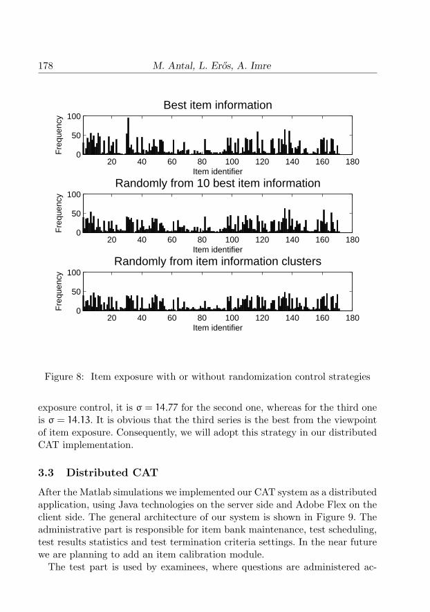
178 M. Antal, L. Eros, A. Imre
20 40 60 80 100 120 140 160 1800
50
100
Item identifier
Fre
quen
cy
Best item information
20 40 60 80 100 120 140 160 1800
50
100
Item identifier
Fre
quen
cy
Randomly from 10 best item information
20 40 60 80 100 120 140 160 1800
50
100
Item identifier
Fre
quen
cy
Randomly from item information clusters
Figure 8: Item exposure with or without randomization control strategies
exposure control, it is σ = 14.77 for the second one, whereas for the third oneis σ = 14.13. It is obvious that the third series is the best from the viewpointof item exposure. Consequently, we will adopt this strategy in our distributedCAT implementation.
3.3 Distributed CAT
After the Matlab simulations we implemented our CAT system as a distributedapplication, using Java technologies on the server side and Adobe Flex on theclient side. The general architecture of our system is shown in Figure 9. Theadministrative part is responsible for item bank maintenance, test scheduling,test results statistics and test termination criteria settings. In the near futurewe are planning to add an item calibration module.
The test part is used by examinees, where questions are administered ac-

Computerized adaptive testing: implementation issues 179
Figure 9: CAT-architecture
cording to settings. After having finished the test, the examinee may viewboth their test results and knowledge report.
3.4 Item difficulty estimation
Due to the lack of measurement data necessary for item calibration, we werenot able to calibrate our item bank. However, 165 out of 171 items of our itembank were used in our self-assessment test system ”Intelligent” in the previousterm. Based on the data collected from this system, we propose a method fordifficulty parameter estimation. Although there were no restrictions in usingthe self-assessment system, i.e. users could have answered an item several

180 M. Antal, L. Eros, A. Imre
20 40 60 80 100 120 140 1600
0.2
0.4
0.6
0.8
1
1.2Item difficulty calibration
Item identifiers
Sca
led
diffi
culti
es
OriginalFirst answers
Figure 10: Item difficulty calibration
times, we consider that the first answer of each user could be relevant to thedifficulty of the item.
Figure 10 shows the original item difficulty (set by the tutor) and the diffi-culty estimated by the first answer of each user. The original data series uses 5difficulty levels scaled to the [0, 1] interval. The elements of the “first answers”series were computed by the equation: all incorrect answersall answers . We computed themean difficulty for both series, and we obtained 0.60 for the original one and0.62 for the estimated one. Conspicuous differences were found at the veryeasy and very difficult item difficulties.
4 Further research
At present we are working on the parameter estimation part of our CATsystem. Although there are several item parameter calibration programs, thistask must be taken very seriously because it influences measurement precision

Computerized adaptive testing: implementation issues 181
directly. Item parameter estimation error is an active research topic, especiallyfor fixed computer tests. For adaptive testing, this problem has been addressedby paper [8].
Researchers have empirically observed that examinees suitable for item dif-ficulty estimations are almost useless when estimating item discrimination.Stocking [14] analytically derived the relationship between the examinee’s abil-ity and the accuracy of maximum likelihood item parameter estimation. Sheconcluded that high ability examinees contribute more to difficulty estima-tion of difficult and very difficult items and less on easy and very easy items.She also concluded that only low ability examinees contribute to the esti-mation of guessing parameter and examinees, who are informative regardingitem difficulty estimation, are not good for item discrimination estimation.Consequently, her results seem to be useful in our item calibration module.
5 Conclusions
In this paper we have described a computer adaptive test system based onItem Response Theory along its implementation issues. Our CAT system wasimplemented after one year experience with a computer based self-assessmentsystem, which proved useful in configuring the parameters of the items. Westarted with the presentation of the exact formulas used by our working CATsystem, followed by some simulations for item selection strategies in order tocontrol item overexposure. We also presented the exact way of item parameterconfiguration based on the data taken from the self-assessment system.
Although we do not present measurements on a working CAT system, theimplementation details presented in this paper could be useful for small insti-tutions planning to introduce such a system for educational measurements ona small scale.
In the near future we would like to add an item calibration module to theadministrative part of the system, taking into account the limited possibilitiesof small educational institutes.

182 M. Antal, L. Eros, A. Imre
References
[1] M. Antal, Sz. Koncz, Adaptive knowledge testing systems, Proc.SZAMOKT XIX, October 8–11, 2009, Tırgu Mures, Romania, pp. 159–164. ⇒176
[2] F. B. Baker, The Basics of Item Response Theory, ERIC Clearinghouseon Assessment and Evaluation, College Park, University of Maryland,2001. ⇒170, 177
[3] M. Barla, M. Bielikova, A. B. Ezzeddinne, T. Kramar, M. Simko, O.Vozar, On the impact of adaptive test question selection for learningefficiency, Computers & Educations, 55, 2 (2010) 846–857. ⇒169
[4] A. Baylari, G. A. Montazer, Design a personalized e-learning system basedon item response theory and artificial neural network approach, ExpertSystems with Applications, 36, 4 (2009) 8013–8021. ⇒169
[5] E. Georgiadou, E. Triantafillou, A. Economides, A review of item expo-sure control strategies for computerized adaptive testing developed from1983 to 2005, Journal of Technology, Learning, and Assessment, 5, 8(2007) 33 p. ⇒175
[6] R. K. Hambleton, R. W. Jones, Comparison of classical test theory anditem response theory and their applications to test development, ITEMS– Instructional Topics in Educational Measurement, 253–262. ⇒169, 170
[7] S. Huang, A content-balanced adaptive testing algorithm for computer-based training systems, in: Intelligent Tutoring Systems (eds. C. Frasson,G. Gauthier, A. Lesgold), Springer, Berlin, 1996, pp. 306–314. ⇒175
[8] W. J. Linden, C. A. W. Glas, Capitalization on item calibration error incomputer adaptive testing, LSAC Research Report 98-04, 2006, 14 p. ⇒181
[9] M. Lilley, T. Barker, C. Britton, The development and evaluation of asoftware prototype for computer-adaptive testing, Computers & Educa-tion, 43, 1–2 (2004) 109–123. ⇒169
[10] F. M. Lord, Application of item response theory to practical testing prob-lems, Lawrence Erlbaum Publishers, NJ, 1980. ⇒171

Computerized adaptive testing: implementation issues 183
[11] G. Rasch, Probabilistic models for some intelligence and attainment tests,Danish Institute for Educational Research, Copenhagen, 1960. ⇒169
[12] L. M. Rudner, An online, interactive, computer adaptive testing tutorial,1998, http://echo.edres.org:8080/scripts/cat/catdemo.htm ⇒170
[13] M. L. Stocking, Controlling item exposure rates in a realistic adaptivetesting paradigm, Technical Report RR 3-2, Educational Testing Service,Princeton, NJ, 1993. ⇒175
[14] M. L. Stocking, Specifying optimum examinees for item parameter esti-mation in item response theory, Psychometrika, 55, 3 (1990) 461–475. ⇒181
[15] H. Wainer, G. L. Kiely, Item clusters and computerized adaptive testing:A case for testlets, Journal of Educational Measurement, 24, 3 (1987)185–201. ⇒175
Received: August 23, 2010 • Revised: November 3, 2010

Acta Univ. Sapientiae, Informatica, 2, 2 (2010) 184–193
Score lists in multipartite
hypertournaments
Shariefuddin PirzadaDepartment of Mathematics, University
of Kashmir, India, and King FahdUniversity of Petroleum and Minerals,
Saudi Arabiaemail: [email protected]
Guofei ZhouDepartment of Mathematics, Nanjing
University, Nanjing, Chinaemail: [email protected]
Antal IvanyiDepartment of Computer Algebra
Eotvos Lorand University, Budapest, Hungaryemail: [email protected]
Abstract. Given non-negative integers ni and αi with 0 ≤ αi ≤ ni
(i = 1, 2, . . . , k), an [α1, α2, . . . , αk]-k-partite hypertournament on∑k
1 ni
vertices is a (k+ 1)-tuple (U1, U2, . . . , Uk, E), where Ui are k vertex setswith |Ui| = ni, and E is a set of
∑k1 αi-tuples of vertices, called arcs, with
exactly αi vertices from Ui, such that any∑k
1 αi subset ∪k1U
′i of ∪k
1Ui, E
contains exactly one of the(∑k
1 αi
)!∑k
1 αi-tuples whose entries belong
to ∪k1U
′i. We obtain necessary and sufficient conditions for k lists of non-
negative integers in non-decreasing order to be the losing score lists andto be the score lists of some k-partite hypertournament.
1 Introduction
Hypergraphs are generalizations of graphs [1]. While edges of a graph are pairsof vertices of the graph, edges of a hypergraph are subsets of the vertex set,
Computing Classification System 1998: G.2.2Mathematics Subject Classification 2010: 05C65Key words and phrases: hypergraph, hypertournament, multi hypertournament, score,losing score.
184

Score lists in multipartite hypertournaments 185
consisting of at least two vertices. An edge consisting of k vertices is calleda k-edge. A k-hypergraph is a hypergraph all of whose edges are k-edges.A k-hypertournament is a complete k-hypergraph with each k-edge endowedwith an orientation, that is, a linear arrangement of the vertices contained inthe hyperedge. Instead of scores of vertices in a tournament, Zhou et al. [13]considered scores and losing scores of vertices in a k-hypertournament, andderived a result analogous to Landau’s theorem [6]. The score s(vi) or si of avertex vi is the number of arcs containing vi and in which vi is not the lastelement, and the losing score r(vi) or ri of a vertex vi is the number of arcscontaining vi and in which vi is the last element. The score sequence (losingscore sequence) is formed by listing the scores (losing scores) in non-decreasingorder.
The following characterizations of score sequences and losing score sequencesin k-hypertournaments can be found in G. Zhou et al. [12].
Theorem 1 Given two positive integers n and k with n ≥ k > 1, a non-decreasing sequence R = [r1, r2, . . . , rn] of non-negative integers is a losingscore sequence of some k-hypertournament if and only if for each j,
j∑i=1
ri ≥(j
k
),
with equality when j = n.
Theorem 2 Given positive integers n and k with n ≥ k > 1, a non-decreasingsequence S = [s1, s2, . . . , sn] of non-negative integers is a score sequence ofsome k-hypertournament if and only if for each j,
j∑i=1
si ≥ j(n− 1
k− 1
)+
(n− j
k
)−
(n
k
),
with equality when j = n.
Some recent work on the reconstruction of tournaments can be found inthe papers due to A. Ivanyi [3, 4]. Some more results on k-hypertournamentscan be found in [2, 5, 9, 10, 11, 13]. The analogous results of Theorem 1 andTheorem 2 for [h, k]-bipartite hypertournaments can be found in [7] and for[α,β, γ]-tripartite hypertournaments in [8].
Throughout this paper i takes values from 1 to k and ji takes values from 1to ni, unless otherwise stated.

186 S. Pirzada, G. Zhou, A. Ivanyi
A k-partite hypergraph is a generalization of k-partite graph. Given non-negative integers ni and αi, (i = 1, 2, . . . , k) with ni ≥ αi ≥ 0 for each i, an[α1, α2, . . . , αk]-k-partite hypertournament (or briefly k-partite hypertourna-ment) M of order
∑k1 ni consists of k vertex sets Ui with |Ui| = ni for each i,
(1 ≤ i ≤ k) together with an arc set E, a set of∑k1 αi-tuples of vertices, with
exactly αi vertices from Ui, called arcs such that any∑k1 αi subset ∪k1U′
i of
∪k1Ui, E contains exactly one of the(∑k
1 αi
) ∑k1 αi-tuples whose αi entries
belong to U′i.
Let e = (u11, u12, . . . , u1α1, u21, u22, . . . , u2α2
, . . . , uk1, uk2, . . . , ukαk), with
uiji ∈ Ui for each i, (1 ≤ i ≤ k, 1 ≤ ji ≤ αi), be an arc in M and let h < t, welet e(u1h, u1t) denote to be the new arc obtained from e by interchanging u1hand u1t in e. An arc containing αi vertices from Ui for each i, (1 ≤ i ≤ k) iscalled an (α1, α2, . . . , αk)-arc.
For a given vertex uiji ∈ Ui for each i, 1 ≤ i ≤ k and 1 ≤ ji ≤ αi, the scored+M(uiji) (or simply d+(uiji)) is the number of
∑k1 αi-arcs containing uiji and
in which uiji is not the last element. The losing score d−M(uiji) (or simply
d−(uiji)) is the number of∑k1 αi-arcs containing uiji and in which uiji is the
last element. By arranging the losing scores of each vertex set Ui separatelyin non-decreasing order, we get k lists called losing score lists of M and theseare denoted by Ri = [riji ]
niji=1
for each i, (1 ≤ i ≤ k). Similarly, by arrangingthe score lists of each vertex set Ui separately in non-decreasing order, we getk lists called score lists of M which are denoted as Si = [siji ]
niji=1
for each i(1 ≤ i ≤ k).
2 Main results
The following two theorems are the main results.
Theorem 3 Given k non-negative integers ni and k non-negative integersαi with 1 ≤ αi ≤ ni for each i (1 ≤ i ≤ k), the k non-decreasing listsRi = [riji ]
niji=1
of non-negative integers are the losing score lists of a k-partitehypertournament if and only if for each pi (1 ≤ i ≤ k) with pi ≤ ni,
k∑i=1
pi∑ji=1
riji ≥k∏i=1
(pi
αi
), (1)
with equality when pi = ni for each i (1 ≤ i ≤ k).

Score lists in multipartite hypertournaments 187
Theorem 4 Given k non-negative integers ni and k non-negative integersαi with 0 ≤ αi ≤ ni for each i (1 ≤ i ≤ k), the k non-decreasing listsSi = [siji ]
niji=1
of non-negative integers are the score lists of a k-partite hyper-tournament if and only if for each pi, (1 ≤ i ≤ k) with pi ≤ ni
k∑i=1
pi∑ji=1
siji ≥
(k∑i=1
αipi
ni
)(k∏i=1
(ni
αi
))+
k∏i=1
(ni − piαi
)−
k∏i=1
(ni
αi
), (2)
with equality when pi = ni for each i (1 ≤ i ≤ k).
We note that in a k-partite hypertournamentM, there are exactly∏ki=1
(niαi
)arcs and in each arc only one vertex is at the last entry. Therefore,
k∑i=1
ni∑ji=1
d−M(uiji) =
k∏i=1
(ni
αi
).
In order to prove the above two theorems, we need the following Lemmas.
Lemma 5 If M is a k-partite hypertournament of order∑k1 ni with score lists
Si = [siji ]niji=1
for each i (1 ≤ i ≤ k), then
k∑i=1
ni∑ji=1
siji =
[(k∑1=1
αi
)− 1
]k∏i=1
(ni
αi
).
Proof. We have ni ≥ αi for each i (1 ≤ i ≤ k). If riji is the losing score ofuiji ∈ Ui, then
k∑i=1
ni∑ji=1
riji =
k∏i=1
(ni
αi
).
The number of [αi]k1 arcs containing uiji ∈ Ui for each i, (1 ≤ i ≤ k), and
1 ≤ ji ≤ ni is
αi
ni
k∏t=1
(nt
αt
).

188 S. Pirzada, G. Zhou, A. Ivanyi
Thus,
k∑i=1
ni∑ji=1
siji =
k∑i=1
ni∑ji=1
(αi
ni
) k∏1
(nt
αt
)−
(ni
αi
)
=
(k∑i=1
αi
)k∏1
(nt
αt
)−
k∏1
(ni
αi
)
=
[(k∑1=1
αi
)− 1
]k∏1
(ni
αi
).
�
Lemma 6 If Ri = [riji ]niji=1
(1 ≤ i ≤ k) are k losing score lists of a k-partitehypertournament M, then there exists some h with r1h < α1
n1
∏k1
(np
αp
)so that
R′1 = [r11, r12, . . . , r1h+1, . . . , r1n1
], R′s = [rs1, rs2, . . . , rst−1, . . . , rsns ] (2 ≤ s ≤
k) and Ri = [riji ]niji=1
, (2 ≤ i ≤ k), i 6= s are losing score lists of some k-partitehypertournament, t is the largest integer such that rs(t−1) < rst = . . . = rsns.
Proof. Let Ri = [riji ]niji=1
(1 ≤ i ≤ k) be losing score lists of a k-partite hyper-tournament M with vertex sets Ui = {ui1, ui2, . . . , uiji} so that d−(uiji) = rijifor each i (1 ≤ i ≤ k, 1 ≤ ji ≤ ni).
Let h be the smallest integer such that
r11 = r12 = . . . = r1h < r1(h+1) ≤ . . . ≤ r1n1
and t be the largest integer such that
rs1 ≤ rs2 ≤ . . . ≤ rs(t−1) < rst = . . . = rsns
Now, letR′1 = [r11, r12, . . . , r1h + 1, . . . , r1n1
],
R′s = [rs1, rs2, . . . , rst − 1, . . . , rsns
(2 ≤ s ≤ k), and Ri = [riji ]niji=1
, (2 ≤ i ≤ k), i 6= s.Clearly, R′
1 and R′s are both in non-decreasing order.
Since r1h < α1n1
∏k1
(np
αp
), there is at least one [αi]
k1-arc e containing both u1h
and ust with ust as the last element in e, let e′ = (u1h, ust). Clearly, R′1, R
′s

Score lists in multipartite hypertournaments 189
and Ri = [riji ]niji=1
for each i (2 ≤ i ≤ k), i 6= s are the k losing score lists ofM′ = (M− e) ∪ e′. �
The next observation follows from Lemma 6, and the proof can be easilyestablished.
Lemma 7 Let Ri = [riji ]niji=1
, (1 ≤ i ≤ k) be k non-decreasing sequences ofnon-negative integers satisfying (1). If r1n1
< α1n1
∏k1
(nt
αt
), then there exists s
and t (2 ≤ s ≤ k), 1 ≤ t ≤ ns such that R′1 = [r11, r12, . . . , r1h + 1, . . . , r1n1
],R′s = [rs1, rs2, . . . , rst−1, . . . , rsns ] and Ri = [riji ]
niji=1
, (2 ≤ i ≤ k), i 6= s satisfy(1).
Proof of Theorem 3. Necessity. Let Ri, (1 ≤ i ≤ k) be the k losing scorelists of a k-partite hypertournament M(Ui, 1 ≤ i ≤ k). For any pi with αi≤ pi ≤ ni, let U′
i = {uiji}piji=1
(1 ≤ i ≤ k) be the sets of vertices such thatd−(uiji) = riji for each 1 ≤ ji ≤ pi, 1 ≤ i ≤ k. Let M′ be the k-partitehypertournament formed by U′
i for each i (1 ≤ i ≤ k).Then,
k∑i=1
pi∑ji=1
riji ≥k∑i=1
pi∑ji=1
d−M′(uiji)
=
k∏1
(ptαt
).
Sufficiency. We induct on n1, keeping n2, . . . , nk fixed. For n1 = α1, theresult is obviously true. So, let n1 > α1, and similarly n2 > α2, . . . , nk > αk.Now,
r1n1=
k∑i=1
ni∑ji=1
riji −
n1−1∑j1=1
r1j1 +
k∑i=2
ni∑ji=1
riji
≤
k∏1
(ntαt
)−
(n1 − 1
α1
) k∏2
(ntαt
)
=
[(n1α1
)−
(n1 − 1
α1
)] k∏2
(ntαt
)
=
(n1 − 1
α1 − 1
) k∏2
(ntαt
).

190 S. Pirzada, G. Zhou, A. Ivanyi
We consider the following two cases.
Case 1. r1n1=
(n1 − 1
α1 − 1
)∏k2
(ntαt
). Then,
n1−1∑j1=1
r1j1 +
k∑i=2
ni∑ji=1
riji =
k∑i=1
ni∑ji=1
riji − r1n1
=
k∏1
(ntαt
)−
(n1 − 1
α1 − 1
) k∏2
(ntαt
)
=
[(n1α1
)−
(n1 − 1
α1 − 1
)] k∏2
(ntαt
)
=
(n1 − 1
α1
) k∏2
(ntαt
).
By induction hypothesis [r11, r12, . . . , r1(n1−1)], R2, . . . , Rk are losing score
lists of a k-partite hypertournament M′(U′1, U2, . . . , Uk) of order
(∑ki=1 ni
)−
1. Construct a k-partite hypertournament M of order∑ki=1 ni as follows. In
M′, let U′1 = {u11, u12, . . . , u1(n1−1)}, Ui = {uiji}
niji=1
for each i, (2 ≤ i ≤k). Adding a new vertex u1n1
to U′1, for each
(∑ki=1 αi
)-tuple containing
u1n1, arrange u1n1
on the last entry. Denote E1 to be the set of all these(n1 − 1
α1 − 1
)∏k2
(ntαt
) (∑ki=1 αi
)-tuples. Let E(M) = E(M′) ∪ E1. Clearly,
Ri for each i, (1 ≤ i ≤ k) are the k losing score lists of M.
Case 2. r1n1<
(n1 − 1
α1 − 1
)∏k2
(ntαt
).
Applying Lemma 7 repeatedly on R1 and keeping each Ri, (2 ≤ i ≤ k) fixeduntil we get a new non-decreasing list R′
1 = [r′11, r′12, . . . , r
′1n1
] in which now
′1n1
=
(n1 − 1
α1 − 1
)∏k2
(ntαt
). By Case 1, R′
1, Ri (2 ≤ i ≤ k) are the losing
score lists of a k-partite hypertournament. Now, apply Lemma 6 on R′1, Ri
(2 ≤ i ≤ k) repeatedly until we obtain the initial non-decreasing lists Ri foreach i (1 ≤ i ≤ k). Then by Lemma 6, Ri for each i (1 ≤ i ≤ k) are the losingscore lists of a k-partite hypertournament. �
Proof of Theorem 4. Let Si = [siji ]niji=1
(1 ≤ i ≤ k) be the k score lists ofa k-partite hypertournament M(Ui, 1 ≤ i ≤ k), where Ui = {uiji}
niji=1
with

Score lists in multipartite hypertournaments 191
d+M(uiji) = siji , for each i, (1 ≤ i ≤ k). Clearly,
d+(uiji) + d−(uiji) = αini
∏k1
(ntαt
), (1 ≤ i ≤ k, 1 ≤ ji ≤ ni).
Let ri(ni+1−ji) = d−(uiji), (1 ≤ i ≤ k, 1 ≤ ji ≤ ni).Then Ri = [riji ]
niji=1
(i = 1, 2, . . . , k) are the k losing score lists of M. Con-versely, if Ri for each i (1 ≤ i ≤ k) are the losing score lists of M, thenSi for each i, (1 ≤ i ≤ k) are the score lists of M. Thus, it is enough toshow that conditions (1) and (2) are equivalent provided siji + ri(ni+1−ji) =(αini
)∏k1
(ntαt
), for each i (1 ≤ i ≤ k and 1 ≤ ji ≤ ni).
First assume (2) holds. Then,
k∑i=1
pi∑ji=1
riji =
k∑i=1
pi∑ji=1
(αi
ni
)( k∏1
(ntαt
))−
k∑i=1
pi∑ji=1
si(ni+1−ji)
=
k∑i=1
pi∑ji=1
(αi
ni
)( k∏1
(ntαt
))−
k∑i=1
ni∑ji=1
riji −
k∑i=1
ni−pi∑ji=1
siji
≥
k∑i=1
pi∑ji=1
(αi
ni
)( k∏1
(ntαt
))−
[((k∑1
αi
)− 1
)k∏1
(niαi
)]
+
k∑i=1
(ni − pi)
(αi
ni
) k∏1
(ntαt
)
+
k∏1
(ni − (ni − pi)
αi
)−
k∏1
(niαi
)
=
k∏1
(niαi
),
with equality when pi = ni for each i (1 ≤ i ≤ k). Thus (1) holds.Now, when (1) holds, using a similar argument as above, we can show that
(2) holds. This completes the proof. �

192 S. Pirzada, G. Zhou, A. Ivanyi
Acknowledgements
The research of the third author was supported by the European Union andthe European Social Fund under the grant agreement no. TAMOP 4.2.1/B-09/1/KMR-2010-0003.
References
[1] C. Berge, Graphs and hypergraphs, translated from French by E. Minieka,North-Holland Mathematical Library 6, North-Holland Publishing Co.,Amsterdam, London, 1973. ⇒184
[2] D. Brcanov, V. Petrovic, Kings in multipartite tournaments and hy-pertournaments, Numerical Analysis and Applied Mathematics: Interna-tional Conference on Numerical Analysis and Applied Mathematics 2009 :1, 2, AIP Conference Proceedings, 1168 (2009) 1255–1257. ⇒185
[3] A. Ivanyi Reconstruction of complete interval tournaments, Acta Univ.Sapientiae Inform., 1, 1 (2009) 71–88. ⇒185
[4] A. Ivanyi, Reconstruction of complete interval tournaments II, Acta Univ.Sapientiae Math., 2, 1 (2010) 47–71. ⇒185
[5] Y. Koh, S. Ree, Score sequences of hypertournament matrices, On k-hypertournament matrices, Linear Algebra Appl., 373 (2003) 183–195.⇒185
[6] H. G. Landau, On dominance relations and the structure of animal soci-eties. III. The condition for a score structure, Bull. Math. Biophys., 15(1953) 143–148. ⇒185
[7] S. Pirzada, T. A. Chishti, T. A. Naikoo, Score lists in [h, k]-bipartitehypertournaments, Discrete Math. Appl., 19, 3 (2009) 321–328. ⇒185
[8] S. Pirzada, T. A. Naikoo, G. Zhou, Score lists in tripartite hypertourna-ments, Graphs and Comb., 23, 4 (2007) 445–454. ⇒185
[9] S. Pirzada G. Zhou, Score sequences in oriented k-hypergraphs, Eur. J.Pure Appl. Math., 1, 3 (2008) 10–20. ⇒185
[10] S. Pirzada, G. Zhou, On k-hypertournament losing scores, Acta Univ.Sapientiae Inform., 2, 1 (2010) 5–9. ⇒185

Score lists in multipartite hypertournaments 193
[11] C. Wang, G. Zhou, Note on degree sequences of k-hypertournaments.Discrete Math., 308, 11 (2008) 2292–2296. ⇒185
[12] G. Zhou, T. Yao, K. Zhang, On score sequences of k-tournaments. Euro-pean J. Comb., 21, 8 (2000) 993–1000. ⇒185
[13] G. Zhou, On score sequences of k-tournaments. J. Appl. Math. Comput.,27 (2008) 149–158. ⇒185
Received: June 23, 2010 • Revised: October 21, 2010

Acta Univ. Sapientiae, Informatica, 2, 2 (2010) 194–209
Pumping lemmas for linear and nonlinear
context-free languages
Dedicated to Pal Domosi on his 65th birthday
Geza HorvathUniversity of Debrecen
email: [email protected]
Benedek NagyUniversity of Debrecen
email: [email protected]
Abstract. Pumping lemmas are created to prove that given languagesare not belong to certain language classes. There are several known pump-ing lemmas for the whole class and some special classes of the context-freelanguages. In this paper we prove new, interesting pumping lemmas forspecial linear and context-free language classes. Some of them can be usedto pump regular languages in two place simultaneously. Other lemma canbe used to pump context-free languages in arbitrary many places.
1 Introduction
The formal language theory and generative grammars form one of the basicsof the field of theoretical computer science [5, 9]. Pumping lemmas play im-portant role in formal language theory [3, 4]. One can prove that a languagedoes not belong to a given language class. There are well-known pumping lem-mas, for example, for regular and context-free languages. The first and mostbasic pumping lemma is introduced by Bar-Hillel, Perles, and Shamir in 1961for context-free languages [3]. Since that time many pumping lemmas are in-troduced for various language classes. Some of them are easy to use/prove,some of them are more complicated. Sometimes a new pumping lemma is in-troduced to prove that a special language does not belong to a given language
Computing Classification System 1998: F.4.3Mathematics Subject Classification 2010: 68Q45Key words and phrases: context-free languages, linear languages, pumping lemma, deriva-tion tree, regular languages
194

Pumping lemmas for linear and nonlinear languages 195
class. Several subclasses of context-free languages are known, such as deter-ministic context-free and linear languages. The linear language class is strictlybetween the regular and the context-free ones. In linear grammars only the fol-lowing types of rules can be used: A → w, A → uBv (A,B are non-terminals,w,u, v ∈ V∗). In the sixties, Amar and Putzolu defined and analysed a specialsubclass of linear languages, the so-called even-linear ones, in which the ruleshas a kind of symmetric shape [1] (in a rule of shape A → uBv, i.e., withnon-terminal at the right hand side, the length of u must equal to the lengthof v). The even-linear languages are intensively studied, for instance, they playspecial importance in learning theory [10]. In [2] Amar and Putzolu extendedthe definition to any fix-rated linear languages. They defined the k-rated lineargrammars and languages, in which the ratio of the lengths of v and u equalsto a fixed non-negative rational number k for all rules of the grammar contain-ing non-terminal in the right-hand-side. They used the term k-linear for thegrammar class and k-regular for the generated language class. In the literaturethe k-linear grammars and languages are frequently used for the metalineargrammars and languages [5], as they are extensions of the linear ones (havingat most k nonterminals in the sentential forms). Therefore, for clarity, we pre-fer the term fix-rated (k-rated) linear for those restricted linear grammars andlanguages that are introduced in [2]. The classes k-rated linear languages arestrictly between the linear and regular ones for any rational value of k. More-over their union the set of all fixed-linear languages is also strictly included inthe class of linear languages. In special case k = 1 the even-linear grammarsand languages are obtained; while the case k = 0 corresponds to the regulargrammars and languages. The derivation-trees of the k-rated linear grammarsform pine tree shapes. In this paper we investigate pumping lemmas for theselanguages also. These new pumping lemmas work for regular languages as well,since every regular language is k-rated linear for every non-negative rationalk. In this way the words of a regular language can be pumped in two placesin a parallel way. There are also extensions of linear grammars. A context-freegrammar is said to be k-linear if it has the form of a linear grammar plus oneadditional rule of the form S → S1S2 . . . Sk, where none of the symbols Si mayappear on the right-hand side of any other rule, and S may not appear in anyother rule at all. A language is said to be k-linear if it can be generated by ak-linear grammar, and a language is said to be metalinear if it is k-linear forsome positive integer k. The metalinear language family is strictly betweenthe linear and context-free ones. In this paper we also introduce a pumpinglemma for not metalinear context-free languages, which can be used to provethat the given language belongs to the class of the metalinear languages.

196 G. Horvath, B. Nagy
2 Preliminaries
In this section we give some basic concepts and fix our notation. Let N denotethe non-negative integers and Q denote the non-negative rationals through thepaper.
A grammar is an ordered quadruple G = (N,V, S,H), where N,V are thenon-terminal and terminal alphabets. S ∈ N is the initial letter. H is a finiteset of derivation rules. A rule is a pair written in the form v → w withv ∈ (N ∪ V)∗N(N ∪ V)∗ and w ∈ (N ∪ V)∗.
Let G be a grammar and v,w ∈ (N∪V)∗. Then v ⇒ w is a direct derivationif and only if there exist v1, v2, v
′, w ′ ∈ (N ∪ V)∗ such that v = v1v′v2, w =
v1w′v2 and v ′ → w ′ ∈ H. The transitive and reflexive closure of ⇒ is denoted
by ⇒∗.The language generated by a grammar G is L(G) = {w|S ⇒∗ w∧w ∈ V∗}.
Two grammars are equivalent if they generate the same language modulo theempty word (λ). (From now on we do not care whether λ ∈ L or not.)
Depending on the possible structures of the derivation rules we are interestedin the following classes [2, 5].• type 1, or context-sensitive (CS) grammars: for every rule the next schemeholds: uAv → uwv with A ∈ N and u, v,w ∈ (N ∪ V)∗, w 6= λ.• type 2, or context-free (CF) grammars: for every rule the next scheme holds:A → v with A ∈ N and v ∈ (N ∪ V)∗.• linear (Lin) grammars: each rule is one of the next forms: A → v, A → vBw;where A,B ∈ N and v,w ∈ V∗.• k-linear (k-Lin) grammars: it is a linear grammar plus one additional ruleof the form S → S1S2 . . . Sk, where S1, S2, . . . , Sk ∈ N, and none of the Si mayappear on the right-hand side of any other rule, and S may not appear in anyother rule at all.• metalinear (Meta) grammars: A grammar is said to be metalinear if it isk-linear for some positive integer k.• k-rated linear (k-rLin) grammars: it is a linear grammar with the followingproperty: there exists a rational number k such that for each rule of the form:A → vBw: |w|
|v| = k (where |v| denotes the length of v).Specially with k = 1:• even-linear (1-rLin) grammars.
Specially with k = 0:• type 3, or regular (Reg) grammars: each derivation rule is one of the followingforms: A → w, A → wB; where A,B ∈ N and w ∈ V∗.
The language family regular/linear etc. contains all languages that can be
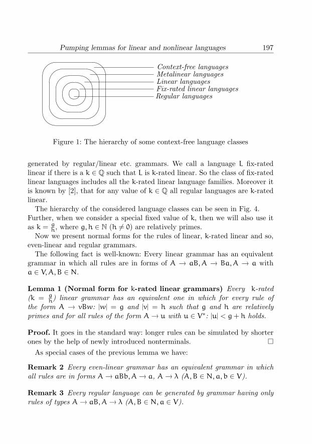
Pumping lemmas for linear and nonlinear languages 197'
&
$
%
'
&
$
%
'
&
$
%������
Context-free languagesMetalinear languagesLinear languagesFix-rated linear languagesRegular languages
Figure 1: The hierarchy of some context-free language classes
generated by regular/linear etc. grammars. We call a language L fix-ratedlinear if there is a k ∈ Q such that L is k-rated linear. So the class of fix-ratedlinear languages includes all the k-rated linear language families. Moreover itis known by [2], that for any value of k ∈ Q all regular languages are k-ratedlinear.
The hierarchy of the considered language classes can be seen in Fig. 4.Further, when we consider a special fixed value of k, then we will also use itas k = g
h , where g, h ∈ N (h 6= 0) are relatively primes.Now we present normal forms for the rules of linear, k-rated linear and so,
even-linear and regular grammars.The following fact is well-known: Every linear grammar has an equivalent
grammar in which all rules are in forms of A → aB,A → Ba,A → a witha ∈ V,A, B ∈ N.
Lemma 1 (Normal form for k-rated linear grammars) Every k-rated(k = g
h) linear grammar has an equivalent one in which for every rule ofthe form A → vBw: |w| = g and |v| = h such that g and h are relativelyprimes and for all rules of the form A → u with u ∈ V∗: |u| < g+ h holds.
Proof. It goes in the standard way: longer rules can be simulated by shorterones by the help of newly introduced nonterminals. �
As special cases of the previous lemma we have:
Remark 2 Every even-linear grammar has an equivalent grammar in whichall rules are in forms A → aBb,A → a, A → λ (A,B ∈ N,a, b ∈ V).
Remark 3 Every regular language can be generated by grammar having onlyrules of types A → aB,A → λ (A,B ∈ N,a ∈ V).

198 G. Horvath, B. Nagy
Derivation trees are widely used graphical representations of derivations incontext-free grammars. The root of the tree is a node labelled by the initialsymbol S. The terminal labelled nodes are leaves of the tree. The nonterminals,as the derivation continues from them, have some children nodes. Since thereis a grammar in Chomsky normal form for every context-free grammar, everyword of a context-free language can be generated such that its derivation treeis a binary tree.
In linear case, there is at most one non-terminal in every level of the tree.Therefore the derivation can go only in a linear (sequential) manner. There isonly one main branch of the derivation (tree); all the other branches terminateimmediately. Observing the derivations and derivation trees for linear gram-mars, they seem to be highly related to the regular case. The linear (and so,specially, the even-linear and fixed linear) languages can be accepted by finitestate machines [1, 7, 8]. Moreover the k-rated linear languages are acceptedby deterministic machines [8].
By an analysis of the possible trees and iterations of nonterminals in aderivation (tree) one can obtain pumping (or iteration) lemmas.
Further in this section we recall some well-known iteration lemmas.The most famous iteration lemma works for every context-free languages [3].
Lemma 4 (Bar-Hillel lemma) Let a context-free language L be given. Thenthere exists an integer n ∈ N such that any word p ∈ L with |p| ≥ n, admits afactorization p = uvwxy satisfying
1. uviwxiy ∈ L for all i ∈ N2. |vx| > 0
3. |vwx| ≤ n.
Example 5 Let L = {aibici | i ∈ N}. It is easy to show with the Bar-Hillellemma that the language L is not context-free.
The next lemma works for linear languages [5].
Lemma 6 (Pumping lemma for linear languages) Let L be a linear lan-guage. Then there exists an integer n such that any word p ∈ L with |p| ≥ n,admits a factorization p = uvwxy satisfying
1. uviwxiy ∈ L for all integer i ∈ N2. |vx| > 0
3. |uvxy| ≤ n.
Example 7 It is easy to show by using Lemma 6 that the languageL = {aibicjdj|i, j ∈ N} is not linear.
Pumping lemmas for linear and nonlinear languages 199
In [6] there is a pumping lemma for non-linear context-free languages thatcan also be effectively used for some languages.
Lemma 8 (Pumping lemma for non-linear context-free languages) LetL be a non-linear context-free language. Then there exist infinite many wordsp ∈ L which admit a factorization p = rstuvwxyz satisfying
1. rsituivwjxyjz ∈ L for all integer i, j ≥ 02. |su| 6= 0
3. |wy| 6= 0.
Example 9 LetH ⊆ {12, 22, 32, . . .}
be an infinite set, and let
LH = {akbkalbl} | k, l ≥ 1; k ∈ H or l ∈ H} ∪ {ambm | m ≥ 1}.
The language LH satisfies the Bar-Hillel condition. Therefore we can notapply the Bar-Hillel Lemma to show that LH is not context-free. However theLH language does not satisfy the condition of the pumping lemma for linearlanguages. Thus LH is not linear. At this point we can apply Lemma 8, and thelanguage LH does not satisfy its condition. This means LH is not context-free.
Now we recall the well-known iteration lemma for regular case (see, forinstance, [5]).
Lemma 10 (Pumping lemma for regular languages) Let L be a regularlanguage. Then there exists an integer n such that any word p ∈ L with |p| ≥ n,admits a factorization p = uvw satisfying
1. uviw ∈ L for all integer i ∈ N2. |v| > 0
3. |uv| ≤ n.
Example 11 By the previous lemma one can easily show that the language{anbn|n ∈ N} is not regular.
Pumping lemmas are strongly connected to derivation trees, therefore theyworks for context-free languages (and for some special subclasses of the context-free languages).
In the next section we present pumping lemmas for the k-rated linear lan-guages and for the not metalinear context-free languages.

200 G. Horvath, B. Nagy
3 Main results
Let us consider a k-rated linear grammar. Based on the normal form (Lemma1) every word of a k = g
h -rated linear language can be generated by a ‘pine-tree’ shape derivation tree (see Fig. 2).
�����
�������
���
�������
���������
@@@
@@
@@@
@@
@@@
@@@
����
BBBB
v2 w2
vn wn
v1 w1
u
S
A1
A2
:
An
Figure 2: A ‘pine-tree’ shape derivation tree in a fix-rated linear grammar
Now we are ready to present our pumping lemmas for these languages.
Theorem 12 Let L be a (gh = k)-rated linear language. Then there exists
an integer n such that any word p ∈ L with |p| ≥ n, admits a factorizationp = uvwxy satisfying
1. uviwxiy ∈ L for all integer i ∈ N2. 0 < |u|, |v| ≤ n h
g+h
3. 0 < |x|, |y| ≤ n gg+h
4. |x||v| =
|y||u| = g
h = k.
Proof. Let G = (N,V, S,H) be a k-rated linear grammar in normal form thatgenerates the language L. Then let n = (|N|+1) · (g+h). In this way any wordp with length at least n cannot be generated without any repetition of a non-terminal in the sentential form. Moreover, by the pigeonhole principle, thereis a nonterminal in the derivation which occurs in the sentential forms duringthe first |N| steps of the derivation and after the first occurrence it occurs also

Pumping lemmas for linear and nonlinear languages 201
�����
������
HHH
HH
������
�����
HHH
HH
HHHH
H
������
�����v x
w
u y
S
A
A
:
:
:
Figure 3: Pumping the subwords between the two occurrences of the non-terminal A.
in the next |N| sentential forms. Considering the first two occurrences of thisnonterminal A in the derivation tree, the word p can be partitioned to fiveparts in the following way. Let u and y be the prefix and suffix (respectively)generated by the first steps till the first occurrence of A. Let v and x be thesubwords that are generated from the first occurrence of A till it appears sec-ondly in the sentential form. Finally let w be the subword that is generatedfrom the second occurrence of A in the derivation. (See also Fig. 3.) In thisway the conditions 2, 3 and 4 of the theorem are fulfilled for the lengths ofthe partitions. Now let us consider the derivation steps between the first twooccurrences of A. They can be omitted from the derivation; in this way theword uwy is obtained. This sequence of steps can also be repeated any time,in this way the words of the form uviwxiy are obtained for any i ∈ N. Thusthe theorem is proved. �
Theorem 13 Let L be a (gh = k)-rated linear language. Then there exists
an integer n such that any word p ∈ L with |p| ≥ n, admits a factorizationp = uvwxy satisfying
1. uviwxiy ∈ L for all integer i ∈ N2. 0 < |v| ≤ n h
g+h
3. 0 < |x| ≤ n gg+h
4. 0 < |w| ≤ n5. |x|
|v| =|y||u| = g
h = k.
Proof. Let G = (N,V, S,H) be a k-rated linear grammar in normal form that

202 G. Horvath, B. Nagy
generates the language L. Then let n = (|N| + 1) · (g + h). In this way anyword p with length at least n cannot be generated without any repetition ofa nonterminal in the sentential form. Moreover there is a nonterminal A inthe derivation which occurs twice among the non-terminals of the last |N+ 1|
sentential forms of the derivation. Considering these last two occurrences ofA in the derivation tree the word p can be partitioned to five parts in thefollowing way. Let u and y be the prefix and suffix (respectively) generatedfrom the first steps till that occurrence of A which is the last but one duringthe derivation. Let v and x be the subwords that are generated by the stepsbetween the last two occurrences of A. Finally let w be the subword that isgenerated from the last occurrence of A in the derivation. In this way theconditions 2, 3, 4 and 5 are fulfilled for the lengths of the partitions. Now letus consider the derivation steps between the these two occurrences of A. Theycan be omitted from the derivation; in this way the word uwy is obtained.This sequence of steps can also be repeated any time, in this way the words ofthe form uviwxiy are obtained for any i ∈ N. Thus the theorem is proved. �
Remark 14 In case of k = 0 the previous theorems give the well-known pump-ing lemmas for regular languages.
Now we are presenting an iteration lemma for another special subclass ofthe context-free language family.
Theorem 15 Let L be a context-free language which does not belong to anyk-linear language for a given positive integer k. Then there exist infinite manywords w ∈ L which admit a factorization w = uv0w0x0y0 . . . vkwkxkyk satis-fying
1. uvi00 w0x
i00 y0 . . . v
ikk wkx
ikk yk ∈ L for all integer i0, . . . , ik ≥ 0
2. |vjxj| 6= 0 for all 0 ≤ j ≤ k.
Proof. Let G = (N,V, S,H) be a context-free grammar such that L(G) = L,and let GA = (N,V,A,H) for all A ∈ N. Because L is not k-linear, there existsA0, . . . , Ak ∈ VN and α,β0, . . . , βk ∈ V∗ such that S ⇒∗ αA0β0 . . . Akβk,where all of the languages L(GAl
), 0 ≤ l ≤ k are infinite. Then the words{α}L(GA0
){β0} . . . L(GAk){βk} ⊆ L, and applying the Bar-Hillel Lemma for
all L(GAl) we receive αa0b
i00 c0d
i00 e0β0 . . . akb
ikk ckd
ikk ekβk ⊆ L for all i0 ≥
0, . . . , ik ≥ 0. Let u = αa0, vl = bl, wl = cl, xl = dl, yl = elβl, and we havethe above form. �

Pumping lemmas for linear and nonlinear languages 203
Remark 16 With k = 1 we have a pumping lemma for non-linear context-freelanguages.
Knowing that every k-linear language is metalinear for any k ∈ N, we have:
Proposition 17 Let L be a not metalinear context-free language. For all in-tegers k ≥ 1 there exist infinite many words w ∈ L which admit a factorizationw = uv0w0x0y0 . . . vkwkxkyk satisfying
1. uvi00 w0x
i00 y0 . . . v
ikk wkx
ikk yk ∈ L for all integer i0, . . . , ik ≥ 0
2. |vjxj| 6= 0 for all 0 ≤ j ≤ k.
4 Applications of the new iteration lemmas
As pumping lemmas are usually used to show that a language does not belongto a language class, we present an example for this type of application.
Example 18 The DYCK language (the language of correct bracket expres-sions) is not k-linear for any value of k over the alphabet {(, )}. Let k 6= 1 befixed as g
h . Let us consider the word of the form ((g+h)(n+2))(g+h)(n+2). ThenTheorem 12 does not work (if k 6= 1), the pumping deletes or introduces dif-ferent number of (’s and )’s. To show that the DYCK language is not 1-rated(i.e., even-)linear let us consider the word (2n)2n(2n)2n. Using Theorem 13 thenumber of inner brackets can be pumped. In this way such words are obtainedin which there are prefixes with more letters ) than (. Since these words do notbelong to the language, this language is not k-linear.
In the previous example we showed that the DYCK language is not fixedlinear.
In the next example we consider a deterministic linear language.
Example 19 Let L = {ambm|m ∈ N} ∪ {amcb2m|m ∈ N} over the alphabet{a, b, c}. Let us assume that the language is fixed linear. First we show that thislanguage is not fixed linear with ratio other than 1. On the contrary, assumethat it is, with k = g
h ∈ Q such that k 6= 1. Let n be given by Theorem 12.Then consider the words of the form am(g+h)bm(g+h) with m > n. By thetheorem any of them can be factorized to uvwxy such that |uv| ≤ 2nh
g+h . Sinceg + h > 2 (remember that g, h ∈ N, relatively primes and g 6= h), |uv| < nh,and therefore both u and v contains only a’s. By a similar argument on thelength of xy, x and y contains only b’s. Since the ratio |x|
|v| (it is fixed by the

204 G. Horvath, B. Nagy
theorem) is not 1, by pumping we get words outside of the language. Now weshow that this language is not even-linear. Assume that it is 1-rated linear(g = h = 1). Let n be the value from Theorem 12. Let us consider the words ofshape amcb2m with m > n. Now we can factorize these words in a way, that|uv| ≤ n and |xy| ≤ n and |v| = |x|. By pumping we get words am+jcb2m+j
with some positive values of j, but they are not in L. We have a contradictionagain. So this language is not fixed linear.
In the next example we show a fixed-linear language that can be pumped.
Example 20 Let L be the language of palindromes, i.e., of the words over{a, b} that are the same in reverse order (p = pR). We show that our pumpinglemmas work for this language with the value k = 1. Let p ∈ L, then p =
uvwxy according to Theorem 12 or Theorem 13, such that |u| = |y| and |v| =
|x|. Therefore, by applying the main property of the palindromes, we have u =
yR, v = xR and w = wR. By i = 0 the word uwy is obtained which is in Laccording to the previous equalities. By further pumping the words uviwxiy
are obtained, they are also palindromes. To show that this language cannotbe pumped with any other values, let us consider words of shape ambam. ByTheorem 12 it can be shown in analogous way that we showed in Example 19that enough long words cannot be pumped with ratio k 6= 1.
Besides our theorems work for regular languages with k = 0 there is a non-standard application of them. As we already mentioned, all regular languagesare k-rated linear for any values of k ∈ Q. Therefore every new pumpinglemma works for any regular language with any values of k. Now we showsome examples.
Example 21 Let the regular language (ab)∗aa(bbb)∗a be given. Then weshow, that our theorems work for, let us say, k = 1
2 . Every word of the lan-guage is of the form (ab)naa(bbb)ma (with n,m ∈ N). For words that arelong enough either n or m (or both of them) are sufficiently large. Now wedetail effective factorizations p = uvwxy of the possible cases. We give onlythose words of the factorization that have maximized lengths due to the ap-plied theorem, the other words can easily be found by the factorization and,at Theorem 13, by taking into account the fixed ratio of some lengths in thefactorization.
• Theorem 12 for k = 12 :
if n > 3 and m > 0 : let u = ab, v = ababab, x = bbb, y = a,if m = 0 : let u = ababab, v = abab, x = ab, y = aaa,

Pumping lemmas for linear and nonlinear languages 205
if n = 3 : let u = abababaa, v = bb, x = b, y = bbba,if n = 2 : let u = ababaa, v = bb, x = b, y = bba,if n = 1 : let u = abaa, v = bb, x = b, y = ba,if n = 0 : let u = aa, v = bb, x = b, y = a.
• Theorem 13 for k = 12 :
if n ≤ 3m− 4 : let v = bb, w = b x = b,if n = 3m− 3 : let v = ababab, w = aabbbb x = bbb,if n = 3m− 2 : let v = ababab, w = abaabbbb x = bbb,if n = 3m− 1 : let v = ababab, w = ababaabbbb x = bbb,if n = 3m : let v = ababab, w = aab x = bbb,if n = 3m+ 1 : let v = ababab, w = abaab, x = bbb,if n = 3m+ 2 : let v = ababab, w = ababaab, x = bbb,if n = 3m+ 3 : let v = ababab, w = abababaab, x = bbb,if n = 3m+ 4 : let v = ababab, w = ababababaab, x = bbb,if n = 3m+ 5 : let v = ababab, w = abababababaab, x = bbb,if n ≥ 3m+ 6, n ≡ 0(mod3) : let v = abab, w = λ, x = ab,if n ≥ 3m+ 7, n ≡ 1(mod3) : let v = abab, w = ab, x = ab,if n ≥ 3m+ 8, n ≡ 2(mod3) : let v = abab, w = abab, x = ab.
In similar way it can be shown that pumping the words of a regular languagein two places simultaneously with other values of k (for instance, 1, 5, 7
3 etc.)works.
In the next example we show that there are languages that can be pumpedby the usual pumping lemmas for regular languages, but they cannot be regularsince we prove that there is a value of k such that one of our theorems doesnot work.
Example 22 Let L = {arbaqbm|r, q,m ≥ 2, ∃j ∈ N : q = j2}. By the usualpumping lemmas for regular languages, i.e., by fixing k as 0, one cannot inferthat this language is not regular. By k = 0, x = y = λ and so p = uvw. Dueto the a’s in the beginning, Theorem 12 works: u = a, v = a; and due to theb’s in the end Theorem 13 also works: v = b,w = b.Now we show that L is not even-linear. Contrary, let us assume that Theorem13 works for k = 1. Let n be the value for this language according to thetheorem. Let p = a2ba(2n+5)2
b3. By the conditions of the theorem, it can befactorized to uvwxy such that |v|, |w|, |x| ≤ n and |u| = |y|. In this way vwxmust be a subword of a(2n+5)2
, and so, the pumping decreases/increases onlyq. Since |v|, |x| ≤ n in the first round of pumping p ′ = a2ba(2n+5)2+|vx|b3 is

206 G. Horvath, B. Nagy
obtained. But (2n + 5)2 < (2n + 5)2 + |vx| ≤ (2n + 5)2 + 2n < (2n + 6)2,therefore p ′ 6∈ L.Thus L is not even-linear, and therefore it cannot be regular. Our pumpinglemma was effective to show this fact.
Usually pumping lemmas can be used only to show that some languagesdo not belong to the given class of languages. One may ask what we can sayif a language satisfy our theorems. Now we present an example which showsthat we cannot infer about the language class if a language satisfies our newpumping lemmas.
Example 23 Let L = {0j1m0r1i0l1i0r1m0j|j,m, i, l, r ≥ 1, r is prime}. Onecan easily show that this language satisfies both Theorem 12 and Theorem 13with k = 1: one can find subwords to pump in the part of outer 0’s or 1’s(pumping their number form a given j or m to arbitrary high values), or inthe middle part 0’s or 1’s (pumping their number from i or l to arbitraryhigh values), respectively. But this language is not even context-free, sinceintersected by the regular language 010∗1010∗10 a non semi-linear languageis obtained. Since context-free languages are semi-linear (due to the Parikhtheorem) and the class of context-free languages are closed under intersectionwith regular languages, we just proved that L cannot be linear or fix-rated linear.
It is a more interesting question what we can say about a language forwhich there are values k1 6= k2 such that all its enough long words can bepumped both as k1-rated and k2-rated linear language. We have the followingconjecture.
Conjecture 24 If a language L satisfies any of our pumping lemmas for twodifferent values of k, then L is regular.
If the previous conjecture is true, then exactly the regular languages form theintersection of the k-rated linear language families (for k ∈ Q).
Regarding iteration lemma for the not metalinear case, we show two exam-ples.
Example 25 This is a very simple example, we can use our lemma to showthat the language
L1 = {alblambmanbn | l,m,n ≥ 0}
is metalinear.

Pumping lemmas for linear and nonlinear languages 207
First of all, it is easy to show that L1 is context-free. The language L1 doesnot satisfy the condition of the pumping lemma for not metalinear context-freelanguages, (Proposition 17,) so L1 must be a metalinear context-free language.
In our next example we show a more complicated language which satisfiesthe Bar-Hillel condition, and we use our pumping lemma to show that thelanguage is not context-free.
Example 26 LetH ⊆ {2k | k ∈ N}
be an infinite set, and let
L2 = {alblambmanbn | l,m, n ≥ 1; l ∈ H or m ∈ H or n ∈ H}∪
∪{aibiajbj | i, j ≥ 1}.
L2 satisfies the Bar-Hillel condition. Therefore we can not apply the Bar-Hillel Lemma to show that L2 is not context-free. However it is easy to showthat L2 is not 3-linear language. Now we can apply Theorem 15, and the lan-guage L2 does not satisfy its condition with k = 3. This means L2 does notbelong to the not 3-linear context-free languages, so the language L2 is notcontext-free.
5 Conclusions
In this paper some new pumping lemmas are proved for special context-freeand linear languages. In fix-rated linear languages the lengths of the pumpedsubwords of a word depend on each other, therefore these pumping lemmasare more restricted than the ones working on every linear or every context-freelanguages. Since all regular languages are k-rated linear for any non-negativerational value of k, these lemmas also work for regular languages. The questionwhether only regular languages satisfy our pumping lemmas at least for twodifferent values of k (or for all values of k) is remained open as a conjecture. Wealso investigated a special subclass of context-free language family and intro-duced iteration conditions which is satisfied only not metalinear context-freelanguages. These conditions can be used in two different ways. First they canbe used to proove that a language is not context-free. On the other hand, wecan also use them to show that the given language is belong to the metalinearlanguage family.

208 G. Horvath, B. Nagy'
&
$
%
'
&
$
%
'
&
$
%����
���
�
�
�
�
�
�
�
�
�
�
�
�
���
����������
Context-sensitive languagesContext-free languagesMetalinear languagesFix-rated linear languages
Figure 4: The target language classes of the new iteration lemmas
Acknowledgements
The work is supported by the Czech-Hungarian bilateral project (TeT) and theTAMOP 4.2.1/B-09/1/KONV-2010-0007 project. The project is implementedthrough the New Hungary Development Plan, co-financed by the EuropeanSocial Fund and the European Regional Development Fund.
References
[1] V. Amar, G. R. Putzolu, On a family of linear grammars, Informationand Control, 7, 3 (1964) 283–291. ⇒195, 198
[2] V. Amar, G. R. Putzolu, Generalizations of regular events, Informationand Control, 8, 1 (1965) 56–63. ⇒195, 196, 197
[3] Y. Bar-Hillel, M. Perles, and E. Shamir, On formal properties of simplephrase structure grammars, Z. Phonetik. Sprachwiss. Komm., 14 (1961)143–172. ⇒194, 198
[4] P. Domosi, M. Ito, M. Katsura, C. Nehaniv, New pumping property ofcontext-free languages, Combinatorics, Complexity an Logic, Proc. Inter-national Conference on Discrete Mathemtics and Theoretical ComputerScience – DMTCS’96, Springer, Singapore, pp. 187–193. ⇒194
[5] J. E. Hopcroft, J. D. Ullman, Introduction to automata theory, languages,and computation, (2nd edition), Addison-Wesley, Reading, MA, 1979. ⇒194, 195, 196, 198, 199
[6] G. Horvath, New pumping lemma for non-linear context-free languages,Proc. 9th Symposium on Algebras, Languages and Computation, ShimaneUniversity, Matsue, Japan, 2006, pp. 160–163. ⇒199

Pumping lemmas for linear and nonlinear languages 209
[7] R. Lokunova, Linear context free languages, Proc. ICTAC 2007, LectureNotes in Comput. Sci., 4711 (2007) 351–365. ⇒198
[8] B. Nagy, On 5 ′ → 3 ′ sensing Watson-Crick finite automata, DNA 13,Revised selected papers, Lecture Notes in Comput. Sci., 4848 (2008)256–262. ⇒198
[9] G. Rozenberg, A. Salomaa, (eds.) Handbook of formal languages, Springer,Berlin, Heidelberg, 1997. ⇒194
[10] J. M. Sempere, P. Garcıa, A characterization of even linear languagesand its application to the learning problem, Proc. Second InternationalColloquium, ICGI-94, Lecture Notes in Artificial Intelligence, 862 (1994)38–44. ⇒195
Received: October 5, 2010 • Revised: November 2, 2010

Acta Univ. Sapientiae, Informatica, 2, 2 (2010) 210–230
Modelling dynamic programming problems
by generalized d-graphs
Zoltan KataiSapientia Hungarian University of TransylvaniaDepartment of Mathematics and Informatics,
Tg. Mures, Romaniaemail: katai [email protected]
Abstract. In this paper we introduce the concept of generalized d-graph(admitting cycles) as special dependency-graphs for modelling dynamicprogramming (DP) problems. We describe the d-graph versions of threefamous single-source shortest algorithms (The algorithm based on thetopological order of the vertices, Dijkstra algorithm and Bellman-Fordalgorithm), which can be viewed as general DP strategies in the case ofthree different class of optimization problems. The new modelling methodalso makes possible to classify DP problems and the corresponding DPstrategies in term of graph theory.
1 Introduction
Dynamic programming (DP) as optimization method was proposed by RichardBellman in 1957 [1]. Since the first book in applied dynamic programmingwas published in 1962 [2] DP has become a current problem solving methodin several fields of science: Applied mathematics [2], Computer science [3],Artificial Intelligence [6], Bioinformatics [4], Macroeconomics [13], etc. Evenin the early book on DP [2] the authors drew attention to the fact that somedynamic programming strategies can be formulated as graph search problems.Later this subject was largely researched. As recent examples: Georgescu andIonescu introduced the concept of DP-tree [7]; Katai [8] proposed d-graphs
Computing Classification System 1998: D.1Mathematics Subject Classification 2010: 68W40, 90C39, 68R10, 05C12Key words and phrases: dynamic programming, graph theory, shortest path algorithms
210

Dynamic programming and d-graphs 211
as special hierarchic dependency-graphs for modelling DP problems; Lew andMauch [14, 15, 16] used specialized Petri Net models to represent DP problems(Lew called his model Bellman-Net).
All the above mentioned modelling tools are based on cycle free graphs.As Mauch [16] states, circularity is undesirable if Petri Nets represent DPproblem instances. On the other hand, however, there are DP problems with“cyclic functional equation” (the chain of recursive dependences of the func-tional equation is cyclic). Felzenszwalb and Zabih [5] in their survey entitledDynamic programming and graph algorithms in computer vision recall thatmany dynamic programming algorithms can be viewed as solving a shortestpath problem in a graph (see also [9, 11, 12]. But, interestingly, some shortestpath algorithms work in cyclic graphs too. Katai, after he has been analyz-ing the three most common single-source shortest path algorithms (The algo-rithm based on the topological order of the vertices, Dijkstra algorithm andBellman-Ford algorithm), concludes that all these algorithms apply cousin DPstrategies [10, 17]. Exploiting this observation Katai and Csiki [12] developedgeneral DP algorithms for discrete optimization problems that can be mod-elled by simple digraphs (see also [11]). In this paper, modelling finite discreteoptimization problems by generalized d-graphs (admitting cycles), we extendthe previously mentioned method for a more general class of DP problems. Thepresented new modelling method also makes possible to classify DP problemsand the corresponding DP strategies in term of graph theory.
Then again the most common approach taken today for solving real-worldDP problems is to start a specialized software development project for everyproblem in particular. There are several reasons why is benefiting to use themost specific DP algorithm possible to solve a certain optimization problem.For instance this approach commonly results in more efficient algorithms. Buta number of researchers in the above mentioned various fields of applicationsare not experts in programming. Dynamic programming problem solving pro-cess can be divided into two steps: (1) the functional equation of the problem isestablished (a recursive formula that implements the principle of the optimal-ity); (2) a computer program is elaborated that processes the recursive formulain a bottom-up way [12]. The first step is reachable for most researchers, butthe second one not necessary. Attaching graph-based models to DP problemsresults in the following benefits:
• it moves DP problems to a well research area: graph theory,• it makes possible to class DP strategies in terms of graph theory,• as an intermediate representation of the problem (that hides, to some

212 Z. Katai
degree, the variety of DP problems) it enables to automate the program-ming part of the problem-solving process by an adequately developedsoftware-tools [12],
• a general software-tool that automatically solves DP problems (gettingas input the functional equation) should be able to save considerablesoftware development costs [16].
2 Modelling dynamic programming problems
DP can be used to solve optimization problems (discrete, finite space) thatsatisfy the principle of the optimality: The optimal solution of the originalproblem is built on optimal sub-solutions respect to the corresponding sub-problems. The principle of the optimality implicitly suggests that the problemcan be decomposed into (or reduced to) similar sub-problems. Usually thisoperation can be performed in several ways. The goal is to build up the optimalsolution of the original problem from the optimal solutions of its smaller sub-problems. Optimization problems can often be viewed as special version ofmore general problems that ask for all solutions, not only for the optimal one(A so-called objective function is defined on the set of sub-problems, whichhas to be optimized). We will call this general version of the problem, all-solutions-version.
The set of the sub-problems resulted from the decomposing process canadequately be modelled by dependency graphs (We have proposed to modelthe problem on the basis of the previously established functional equationthat can be considered the output of the mathematical part and the inputof the programming part of the problem solving process). The vertices (con-tinuous/dashed line squares in the optimization/all-solutions version of theproblem; see Figures 2.a,b,c) represent the sub-problems and directed arcs thedependencies among them. We introduce the following concepts:
• Structural-dependencies: We have directed arc from vertex A to vertexB if solutions of sub-problem A may directly depend on solutions of sub-problem B (dashed arcs; see Figure 2.a).
• Optimal-dependencies: We have directed arc from vertex A to vertex Bif the optimal solution of sub-problem A directly depends on the optimalsolution of the smaller (respect to the optimization process) sub-problemB (continuous arcs; see Figure 2.b).
• Optimization-dependencies: We have directed arc from vertex A to ver-tex B if the optimal solutions of sub-problem A may directly depend on

Dynamic programming and d-graphs 213
the optimal solution of the smaller (respect to the optimization process)sub-problem B (dotted arcs; see Figure 2.c).
Since structural dependencies reflect the structure of the problem, the struc-tural-dependencies-graph can be considered as input information (It can bebuilt up on the basis of the functional equation of the problem). This graphmay contain cycles (see Figure 2.a). According to the principle of the optimal-ity the optimal-dependencies-graph is a rooted sub-tree (acyclic sub-graph) ofthe structural-dependencies-graph. Representing the structure of the optimalsolution the optimal-dependencies-graph can be viewed as output informa-tion. Since optimization-dependencies are such structural-dependencies thatare compatible with the principle of the optimality, the optimization-dependen-cies-graph is a maximal rooted sub-tree of the structural-dependencies-graphthat includes the optimal-dependencies-tree. Accordingly, the vertices of theoptimization-dependencies-graph (and implicitly the vertices of the optimal-dependencies-graph too) can be arranged on levels (hierarchic structure) insuch a way that all its arcs are directed downward. The original problem (orproblem-set) is placed on the highest level and the trivial ones on the lowestlevel. We consider that a sub-problem is structurally trivial if cannot be de-composed into, or reduced to smaller sub-sub-problems. A sub-problem is con-sidered to be trivial regarding the optimization process if its optimal solutiontrivially results from the input data. If the structural-dependencies-graph con-tains cycles, then completing the hierarchic optimization-dependencies-graphto the structural-dependencies-graph some added arcs will be directed upward.
Let us consider, as an example, the following problem: Given the weightedundirected triangle graph OAB determine
• all paths from vertex O (origin) to the all vertices (O, A, B) of the graph(Figure 1.a),
• the maximal length paths from vertex O (origin) to the all vertices ofthe graph (|OA| = 10, |OB| = 10, |AB| = 100) (Figure 1.b),
• the minimal length paths from vertex O (origin) to the all vertices of thegraph (|OA| = 100, |OB| = 10, |AB| = 10) (Figure 1.c).
Since path (O,A,B) includes path (O,A) and, conversely, path (O,B,A) in-cludes path (O,B) the structural-dependencies-graph that can be attached tothe problem is not cycle free (Figure 2.a). We have bidirectional arcs betweenvertices representing sub-problems A (determine all paths to vertex A) and B(determine all paths to vertex B). Since the maximizing version of the prob-lem does not satisfy the principle of the optimality (the maximal path (O,B,A)

214 Z. Katai
uA uB@@@@@u
O
�����
(a)
uA uB@@@@@u
O
��
���
100
10 10
(b)
uA uB@@@@@u
O
���
��
10
100 10
(c)
Figure 1: The triangle graph
includes path (O,B) that is not a maximal path too), in case b the optimal-dependencies-tree and the optimization-dependencies-tree are not defined. Fig-ures 2.b and 2.c present the optimal- and optimization-dependencies-graphsattached to the minimizing version of the problem.
Figure 2: Structural/Optimal/Optimization-dependencies-graphs
3 d-graphs as special dependency graphs
Since decomposing usually means that the current problem is broken downinto two or more immediate sub-problems (1 → N dependency) and sincethis operation can often be performed in several ways, Katai [8] introducedd-graphs as special dependency graphs for modelling such problems. In thispaper we define a generalized form of d-graphs as follows:

Dynamic programming and d-graphs 215
Definition 1 The connected weighted bipartite finite digraph Gd(V, E, C) is ad-graph if:
• V = Vp⋃
Vd and E = Ep⋃
Ed, where
– Vp is the set of the p-vertices,
– Vd is the set of the d-vertices,
– all in/out neighbours of the p-vertices (excepting the source/sinkvertices) are d-vertices; each d-vertex has exactly one p-in-neighbour;each d-vertex has at least one p-out-neighbour,
– Ep is the set of p-arcs (from p-vertices to d-vertices),
– Ed is the set of d-arcs (from d-vertices to p-vertices),
• function C : Ep → R associates a cost to every p-arc. We consider d-arcsof zero cost.
If a d-graph is cycle-free, then its vertices can be arranged on levels (hi-erarchic structure) (see Figure 3). In [8] Katai defines, respect to hierarchicd-graphs, the following related concepts: d-sub-graph, d-tree, d-sub-tree, d-spanning-tree, optimal d-spanning-tree and optimally weighted d-graph.
4 Modelling optimization problems by d-graphs
According to Katai [8] a hierarchic d-graph can be viewed as representing theoptimization-dependences-graph corresponding to the original problem and d-sub-graphs to the sub-problems. Since there is a one-to-one correspondencebetween p-vertices and d-sub-graph [8], these vertices also represent the sub-problems. The source p-vertex (or vertices) is attached to the original problem(or original problem-set), and the sink vertices to the structurally trivial sub-problems. A p-vertex has as many d-sons as the number of possibilities todecompose the corresponding sub-problem into its smaller immediate sub-sub-problems. A d-vertex has as many p-sons as the number of immediatesmaller sub-problems (N) resulted through the corresponding breaking-downstep (1 → N dependency between the p-grandfather-problem and the corre-sponding p-grandson-problems). We will say that a grandfather-problem isreduced to its grandson-problem if the intermediary d-vertex has a single p-son (1 → 1 dependency). Parallel decomposing processes may result in iden-tical sub-problems, and, consequently, the corresponding p-vertex has multi-ple p-grandfathers (through different d-fathers). Due to this phenomenon the

216 Z. Katai
Figure 3: Hierarchic d-graph. p- and d-vertices are represented by rectanglesand circles, respectively (We used bolded lines to emphasize the optimal d-spanning-(sub)trees)
number of the sub-problems may depend on the size of the input polynomi-ally. The d-spanning-trees of the d-(sub)graphs represent the corresponding(sub)solutions, more exactly their tree-structure. The number of all solutionsof the problem usually depends on the size of the input exponentially.
For example, if a p-vertex has n d-sons, these d-sons have m1, m2, . . . , mn p-sons, and these p-son-problems have (r1,1, r1,2, . . . , r1,m1), (r1,1, r1,2, . . . , r1,m2),
(r1,1, r1,2, . . . , r1,mn) solutions, respectively, then from the∑ ∑
rij solution ofthe p-grandson-problems results
∑ ∏rij solution for the common p-grandfa-
ther-problem. The number of solutions exponentially exceeds the number ofsub-problems. The
∑-operator reflects the OR-connection between d-brothers
and the∏
-operator the AND-connection between p-brothers.
5 Dynamic programming strategy on theoptimization-dependencies d-graph
In the case of optimization problems we are interested only in the optimalsolution of the original problem. Dynamic programming means building up

Dynamic programming and d-graphs 217
the optimal solutions of the larger sub-problems from the optimal solutionof the already solved smaller sub-problems (starting with the optimal solu-tion of the trivial sub-problems). Accordingly, (1) DP works on the hierarchicoptimization-dependencies d-graph that can be attached to the problem, and(2) it deals with one solution per sub-problem, with the optimal one (DPstrategies usually result in polynomial algorithms).
In line with this Katai [8] defines two weight-functions (wp : Vp → R, wd :
Vd → R) on the sets of p- and d-vertices of the attached hierarchic d-graph.Whereas the weight of a p-vertex is defined as the optimum (minimum/maxi-mum) of the weights of its d-sons, the weight of a d-vertex is a function (de-pending on the problem to be modelled) of the weights of its p-sons. We con-sider the weight of a d-vertex to be optimal if is based on optimal the weightsof its p-sons. The optimal weight of a p-vertex (excluding the sink vertices)is equal with the minimum/maximum of the optimal weights of its d-sons.The optimal weights of the p-sinks trivially result from the input data of theproblem. Accordingly: the optimal weights of the p-vertices are computed (1)in optimal way, (2) on the basis of the optimal weights of their p-descendents.This means bottom-up strategy. Computing the optimal weights of the p-vertices we implicitly have their optimal d-sons (It is characteristic to DPalgorithms that during the bottom-up building process it stores the alreadycomputed optimal p-weights in order to have them at hand in case they areneeded to compute further optimal p-weights. If we also store the optimal d-sons of the p-vertices, then this information allows a quick reconstruction ofthe optimal d-spanning-tree in top-down way [17, 18]).
Defining the costs of the p-arcs as the absolute value of the weight-differenceof its endpoints we get an optimally weighted d-graph with zero-cost mini-mal d-spanning-tree. We denote these kinds of p-arc-cost-functions by C∗ [8].Modelling optimization problems by a d-graphs Gd(V, E, C∗) includes choosingfunctions wp and wd in such a way as the optimal weights of the p-vertices torepresent the optimum values of the objective function respect to the corre-sponding sub-problems (These functions can be established on the basis of thefunctional equation of the problem; input information regarding the modellingprocess).
Proposition 2 If an optimization problem can be modelled by a hierarchicd-graph Gd(V, E, C∗) (as we described above), then it can be solved by dynamicprogramming.
Proof. Since in an optimally weighted d-graph d-sub-trees of an optimal d-spanning-tree are also optimal d-spanning-trees respect to the d-sub-graphs

218 Z. Katai
defined by their root-vertices, computing the optimal p- and d-weights ac-cording to a reverse topological order of the vertices (based on optimization-dependencies) implicitly identifies the optimal d-spanning-tree of the d-graph.This bottom-up strategy means DP and the optimal solution of the originalproblem will be represented by the weight of the source vertex (as value) andby the minimal d-spanning-tree (as structure). �
Computing the optimal weight of a p-vertex (expecting vertices representingtrivial sub-problems) can be implemented as a gradual updating process basedon the weights of its d-sons. The weights of p-vertices representing trivialsub-problems receive as starting-value their input optimal value. For otherp-vertices we choose a proper starting-value according to the nature of theoptimization problem (The weights of d-vertices are recomputed before everyuse). We define the following types of updating operations along p-arcs (if theweight of a certain d-son is “better” than the weight of his p-father, then thefather’s weight is replaced with the son’s weight):
• Complete: based on the optimal value of the corresponding d-son.• Partial: based on an intermediate value of the corresponding d-son.• Effective: effectively improves the weight of the corresponding p-vertex.• Null: dose not adjusts the weight of the corresponding p-vertex.• Optimal: sets the optimal weight for the corresponding p-vertex. Optimal
updates are complete and effective too.
6 d-graph versions of three famous single-sourceshortest-path algorithms
As we mentioned above, Katai concludes that the three famous single-sourceshortest-path algorithms in digraphs (The algorithm based on the topologicalorder of the vertices, Dijkstra algorithm and Bellman-Ford algorithm) applycousin DP strategies [10, 17]. The common representative core of these DPalgorithms is that the optimal weights (representing the optimal lengths tothe corresponding vertices) are computed on account of updating these valuesalong the arcs of the shortest-paths-tree according to their topological order(optimal-updating-sequence). Since this optimal tree is unknown (it repre-sents the solution of the problem) all the three algorithms generate updating-sequences which contain, as subsequence, an optimal-updating-sequence nec-essary for the dynamic programming building process. The basic difference

Dynamic programming and d-graphs 219
4(4) 1(1)
2(2)
3(3)
5(6) 6(5)
50(1) 100(4)
10(7)
40(8)
80(11)
50(5) 150(9) 60(6)
120(3) 30(10)
110(2) [0]
[50]
[110] [100]
[150]
[160]
4(6) 1(1)
2(2)
5(3) 6(4)
50(1)
100(4)
10(8)
40(9)
80(7)
50(5) 150(10)
60(6)
120(3) 30(11)
110(2) [0]
[50]
[110] [100]
[150]
[160]
4(6):2 1(1):0
2(2):1
3(4):2
5(5):2 6(3):2
50(9):1
100(5):2
10(8):2
40(7)
80(4)
50(6):2 150(10)
60(1):2
120(3) 30(11)
110(2) [0]
[50]
[110] [100]
[150]
[160]
(1,2), (1,5), (1,6), (2,3), (2,5), (2,6), (3,4), (3,5), (3,6), (4,5), (6,5)
(1,2), (1,5), (1,6), (2,3), (2,5), (2,6), (6,5), (3,4), (3,5), (3,6), (4,5)
1: (2,6), (1,5), (1,6), (6,5), (2,3), (2,5), (3,5), (3,4), (1,2), (3,6), (4,5)
2: (2,6), (1,5), (1,6), (6,5), (2,3), (2,5), (3,5), (3,4), (1,2), (3,6), (4,5)
3(5)
Figure 4: The strategies of the (a) Topological, (b) Dijkstra and (c) Bellman-Ford algorithms (we bolded the optimal-arc-subsequence of the generated arc-sequences)

220 Z. Katai
among the three algorithms is the way they generate a proper arc-sequenceand the corresponding updating-sequence.
In case the input digraph is acyclic we get a proper arc-sequence by orderingall the arcs of the graph topologically (this order can even be determined inadvance). Dijkstra algorithm (working in cyclic graphs too, but without neg-ative weighted arcs) determines the needed arc-sequence on the fly (parallelwith the updating process). After the current weight of the next closest vertexhas been confirmed as optimal value (greedy decision), the algorithm performsupdating operations along the out-arcs of this vertex (This greedy choice canbe justified as follows: if other out-neighbours of the growing shortest-paths-tree are farther - from the source vertex - than the currently closest one, thenthrough these vertices cannot lead shortest paths to this). Bellman-Ford algo-rithm (working in cyclic graphs with negative weighted arcs too, but withoutfeasible negative weighted cycles) goes through (in arbitrary order) all thearcs of the graph again and again until the arc-sequence generated in this wayfinally will contains, as sub-sequence, an optimal-updating-sequence (see Fig-ure 4, [10]). The following d-graph algorithms implement DP strategies thatexploit the core idea behind the above described single-source shortest-pathsalgorithms.
6.1 Building-up the optimization-dependencies d-graph inbottom-up way
Our basic goal is to perform updating operation along the p-arcs of theoptimal-dependencies-tree according to their reverse topological order. We willcall such arc sequences optimal-arc-sequence and the corresponding updatingsequences optimal-updating-sequence. An optimal-updating-sequence surelyresults in building up the optimal value representing the optimal solution ofthe problem. Since the optimal-dependencies-tree is unknown (it representsthe structure of the optimal solution to be determined), we should try toelaborate complete arc sequences that includes the desired optimal-updating-sequence (gratuitous updating operations have, at the worst, null effects).
We introduce the following colouring-convention:
• Initially all vertices are white.• A p-vertex changes its colour to grey after the first attempt to update
its weight. d-vertices automatically change their colour to grey if theydo not have any more white p-sons.
• When the weight of a vertex riches its optimal value its colour is auto-matically changed to black.

Dynamic programming and d-graphs 221
We are facing a gratuitous updating operation if:
• along the corresponding p-arc was previously performed a complete up-date,
• the corresponding p-father is already black,• the corresponding d-son is still grey or white.
Since the optimal values of trivial sub-problems automatically results fromthe input data of the problem, the corresponding p-vertices are automaticallycoloured with black.
The following propositions can be viewed as theoretical support for the be-low strategies that build up the optimal-dependencies d-graph (on the basis ofthe structural-dependencies-graph that can be considered input information)level-by-level in bottom-up way (At the beginning all p-vertices are places atlevel 0. All effective updates along the corresponding p-arcs move their p-endto higher level than the highest p-son of their d-end.).
Proposition 3 If the structural-dependencies d-graph attached to an opti-mization problem that satisfies the principle of the optimality has no blackp-sources, then there exists at least one p-arc corresponding to an effectivecomplete updating operation.
Proof. Since the optimization problem satisfies the principle of the optimalitythe optimal-updating-sequence there exists and continuously warrants (whileno black p-sources still exist) the existence of optimal updating operations,which are effective and complete too. �
Proposition 4 Any p-arcs sequence (of the structural-dependencies d-graphattached to an optimization problem that satisfies the principle of the optimal-ity) that continuously applies non-repetitive complete updates (while such up-dating operations still exist) warrants that all p-sources become black-coloured.These p-arcs sequences contain arcs representing optimization-dependenciesand surely include an optimal-arc-sequence.
Proof. Since the optimization problem satisfies the principle of the optimal-ity the optimal-updating-sequence there exists and warrants the continuousexistence of optimal updating operations (which are also effective and com-plete) while no black p-sources still exist. Accordingly any p-arcs sequence thatcontinuously applies non-repetitive complete updates includes an optimal-arc-sequence, and consequently results in colouring all p-sources with black. �

222 Z. Katai
Proposition 5 If the structural-dependencies d-graph attached to an opti-mization problem that satisfies the principle of the optimality is cycle-free,then any reverse topological order of the all p-arcs continuously applies non-repetitive complete updates, and consequently, results in building up the optimalsolution of the problem.
Proof. Since the colours of the d-vertices surely become black after all their p-sons have already become black, any reverse topological order of all p-arcs con-tinuously applies non-repetitive complete updates. According to the previousproposition these arc-sequences surely include an optimal-arc-sequence, andconsequently results in building up the optimal solution of the problem. �
Proposition 6 If an optimization problem satisfies the principle of the op-timality, then there exists a finite multiple complete arc-sequence of the at-tached structural-dependencies d-graph that includes an optimal-arc-sequence,and consequently, the corresponding updating-sequence results in building upthe optimal solution of the problem.
Proof. The existence of such an arc-sequence immediately results from thefacts that: (1) Any complete arc-sequence contains all arcs of the optimal-dependencies-tree; (2) The optimal-dependencies-tree is finite. If we repeat acomplete arc-sequence that includes the arcs of the optimal-dependencies-treeaccording to their topological order (worst case), then we need as many upda-ting-tours as the number of the p-arcs of the optimal-dependencies-tree is.�
6.1.1 Algorithm d-TOPOLOGICAL
If the structural-dependencies d-graph attached to the problem is cycle free(called: structurally acyclic DP problems), then this input graph can also beviewed as optimization-dependencies-graph. Considering a reverse topologicalorder of the all vertices, all updating operations (along the corresponding p-arc-sequence) will be complete (see Proposition 5). Additionally, along thearcs of the optimal d-spanning-tree we have optimal updates. Accordingly,this algorithm (called d-TOPOLOGICAL) results in determining the optimalsolution of the problem.
6.1.2 Algorithm d-DIJKSTRA
If the structural-dependencies d-graph contains cycles a proper vertices or-der involving complete updates along the corresponding p-arc-sequence can-

Dynamic programming and d-graphs 223
not be structurally established. In this case we should try to build up theoptimization-dependencies d-graph (more exactly a reverse topological orderof its all p-arcs) on the fly, parallel with the bottom-up optimization process.
Implementing a sequence of continuous complete updates presumes to iden-tify at each stage of the building process the black d-vertices based on whichwe have not performed complete updating operations (Proposition 3 guar-anties that such d-vertices exist continuously). A d-vertex is black only ifall its p-sons are already black. Consequently, the basic question is: Can weidentify the black p-vertices at each stage of the building process? As we men-tioned above a p-vertex is certainly black after we have performed completeupdates based on all its d-sons (The last effective update was performed onthe basis of optimal d-son). Algorithms based on the topological order of theall arcs exploit this structural condition. However, a p-vertex may have be-come black before we have performed complete updating operation along allits p-out-arcs. Conditions making perceptible such black p-vertices may alsobe deduced from the principle of the optimality. For example, if the DP prob-lem has a greedy character too, then it may work the following condition: the“best” d-vertex (having relatively optimal weight) among those based on whichwe have not performed complete updating operations can be considered black(Called: Cyclic DP problems characterized by greedy choices). Since Dijkstraalgorithm applies this strategy, we call this algorithm: d-DIJKSTRA.
6.1.3 Algorithm d-BELLMAN-FORD
If we cannot establish one complete arc-sequence including an optimal-arc-sequence (we will call such problems: DP problems without ’negative cycles’),we are forced to repeat the updating-tour along a complete (even arbitrary)arc-sequence of the input graph (structural-dependencies d-graph) until thismultiple arc-sequence will include the desired optimal updating sequence (seeProposition 6). An extra tour without any effective updates indicates thatthe optimal solution has been built up. If the arbitrary arc-sequence we havechosen includes the arcs of the optimal-dependencies-tree in topological order(worst case), then we need as many updating-tours as the number of the p-arcsof the optimal-dependencies-tree is. Since Bellman-Ford algorithm applies thisstrategy, we call this algorithm: d-BELLMAN-FORD.
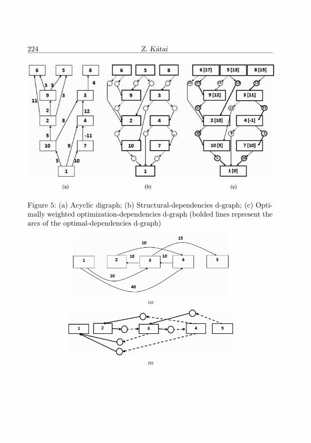
224 Z. Katai
Figure 5: (a) Acyclic digraph; (b) Structural-dependencies d-graph; (c) Opti-mally weighted optimization-dependencies d-graph (bolded lines represent thearcs of the optimal-dependencies d-graph)
(a)
(b)

Dynamic programming and d-graphs 225
Figure 6: (a) Cyclic digraph without negative weighted arcs; (b) Cyclicstructural-dependencies d-graph; (c) The bottom-up building-up process ofthe optimally weighted optimization-dependencies d-graph (bolded lines rep-resent the arcs of the optimal-dependencies d-graph)

226 Z. Katai

Dynamic programming and d-graphs 227
Figure 7: (a) Cyclic digraph with negative weighted arcs, but without negativecycles; (b) Cyclic structural-dependencies d-graph; The bottom-up building-upprocess of the optimally weighted optimization-dependencies d-graph (boldedlines represent the arcs of the optimal-dependencies d-graph): (c1–c4) firstupdating-tour, (d) second updating-tour

228 Z. Katai
6.1.4 A relevant sample problem
As an example we consider the single-source shortest problem: Given a weighteddigraph determine the shortest paths from a source vertex to all the othervertices (destination vertices). The attached figures (see Figures 5, 6, 7) il-lustrate the level by level building process of the optimization-dependenciesd-graph concerning to the algorithms d-TOPOLOGICAL, d-DIJKSTRA andd-BELLMAN-FORD (Regarding this problem we have only 1 → 1 dependen-cies between neighbour p-vertices).
7 Conclusions
Introducing the generalized version of d-graphs we received a more effectivetool for modelling a larger class of DP problems (Hierarchic d-graphs intro-duced in [8] and Petri-net based models [14, 15, 16] work only in the case ofstructurally acyclic problems; Classic digraphs [11, 12] can be applied whenduring the decomposing process at each step the current problem is reducedto only one sub-problem). The new modelling method also makes possibleto classify DP problems (Structurally acyclic DP problems; Cyclic DP prob-lems characterized by greedy choices; DP problems without ’negative cycles’)and the corresponding DP strategies (d-TOPOLOGICAL, d-DIJKSTRA, d-BELLMAN-FORD) in term of graph theory.
If we have proposed to develop a general software-tool that automaticallysolves DP problems (getting as input the functional equation) we should com-bine the above algorithms as follows:
• We represent explicitly the d-graph described implicitly by the functionalequation.
• We try to establish the reverse topological order of the vertices by a DFSlike algorithm (d-DFS). This algorithm can also detect possible cycles.
• If the graph is cycle free, we apply algorithm d-TOPOLOGICAL, elsewe try to apply algorithm d-DIJKSTRA.
• If no mathematical guarantees that we reached the optimal solution, thenchoosing as complete arc-sequence for algorithm d-BELLMAN-FORDthe arc-sequence generated by algorithm d-DIJKSTRA (completed withunused arcs) in the first updating-tour we verify the d-DIJKSTRA result.We repeat the updating tours until no more effective updates.
Such a software-application should be able to save considerable softwaredevelopment costs.

Dynamic programming and d-graphs 229
8 Acknowledgements
This research was supported by the Research Programs Institute of SapientiaFoundation, Cluj, Romania.
References
[1] R. Bellman, Dynamic programming, Princeton University Press, Prince-ton, NJ, 1957. ⇒210
[2] R. Bellman, S. Dreyfus, Applied dynamic programming, Princeton Uni-versity Press, Princeton, NJ, 1962. ⇒210
[3] T. H. Cormen, C. E. Leiserson, R. L. Rivest, C. Stein, Introduction toalgorithms, 3rd edition, The MIT Press, Cambridge, MA, USA, 2009. ⇒210
[4] R. Durbin, S. Eddy, A. Krogh, G. Mitchison, Biological sequence analysis,Cambridge University Press, Cambridge, UK, 1998. ⇒210
[5] P. F. Felzenszwalb, R. Zabih, Dynamic programming and graph algo-rithms in computer vision, IEEE Transactions on Pattern Analysis andMachine Intelligence, Preprint, 19 July 2010, 51 p.http://doi.ieeecomputersociety.org/10.1109/TPAMI.2010.135 ⇒211
[6] Z. Feng, R. Dearden, N Meuleau, R. Washington, Dynamic programmingfor structured continuous Markov decision problems, Proc. 20th Confer-ence on Uncertainty in Artificial Intelligence, ACM International Con-ference Proceeding Series, AUAI Press, 70 (2004) pp. 154–161. ⇒210
[7] H. Georgescu, C. Ionescu, The dynamic programming method, a newapproach, Studia Univ. Babes-Bolyai Inform., 43, 1 (1998) 23–38. ⇒210
[8] Z. Katai, Dynamic programming and d-graphs, Studia Univ. Babes-BolyaiInform., 51, 2 (2006) 41–52. ⇒210, 214, 215, 217, 228
[9] Z. Katai, Dynamic programming strategies on the decision tree hiddenbehind the optimizing problems, Informatics in Education, 6, 1 (2007)115–138. ⇒211
[10] Z. Katai, The single-source shortest paths algorithms and the dynamicprogramming, Teaching Mathematics and Computer Science, 6, SpecialIssue (2008) 25–35. ⇒211, 218, 220

230 Z. Katai
[11] Z. Katai, Dynamic programming as optimal path problem in weighteddigraphs, Acta Math. Acad. Paedagog. Nyhazi, 24, 2 (2008) 201–208. ⇒211, 228
[12] Z. Katai, A. Csiki, Automated dynamic programming, Acta Univ. Sapi-entiae Inform., 1, 2 (2009) 149–164. ⇒211, 212, 228
[13] I. King, A simple introduction to dynamic programming in macroeco-nomic models, 2002.http://researchspace.auckland.ac.nz/bitstream/handle/2292/190/230.pdf⇒210
[14] A. Lew, A Petri net model for discrete dynamic programming, Proc. 9thBellman Continuum: International Workshop on Uncertain Systems andSoft Computing, Beijing, China, July 24–27, 2002, pp. 16–21. ⇒211, 228
[15] A. Lew, H. Mauch, Bellman nets: A Petri net model and tool for dy-namic programming, Proc. 5th Int. Conf. Modelling, Computation andOptimization in Information Systems and Management Sciences (MCO),Metz, France, 2004, pp. 241–248. ⇒211, 228
[16] H. Mauch, DP2PN2Solver: A flexible dynamic programming solver soft-ware tool, Control Cybernet., 35, 3 (2006) 687–702. ⇒211, 212, 228
[17] M. Sniedovich, Dijkstra’s algorithm revisited: the dynamic programmingconnexion, Control Cybernet., 35, 3 (2006) 599–620. ⇒211, 217, 218
[18] D. Vagner, Power programming: dynamic programming, The Mathemat-ica Journal, 5, 4 (1995) 42–51. ⇒217
Received: September 1, 2010 • Revised: November 10, 2010

Contents
Volume 2, 2010
S. Pirzada, G. ZhouOn k-hypertournament losing scores . . . . . . . . . . . . . . . . . . . . . . . . . . . . 5
P. Burcsi, A. Kovacs, A. TatraiStart-phase control of distributed systems written inErlang/OTP . . . . . . . . . . . . . . . . . . . . . . . . . . . . . . . . . . . . . . . . . . . . . . . . . . . 10
S. Korecko, B. SobotaUsing Coloured Petri Nets for design of parallel raytracingenvironment . . . . . . . . . . . . . . . . . . . . . . . . . . . . . . . . . . . . . . . . . . . . . . . . . . . 28
P. Vaclavık, J. Poruban, M. MezeiAutomatic derivation of domain terms and concept locationbased on the analysis of the identifiers . . . . . . . . . . . . . . . . . . . . . . . . . 40
A. AchsA multivalued knowledge-base model . . . . . . . . . . . . . . . . . . . . . . . . . . 51
P. Fornai, A. IvanyiFIFO anomaly is unbounded . . . . . . . . . . . . . . . . . . . . . . . . . . . . . . . . . . . 80
B. Sobota, M. GuzanMacro and micro view on steady states in state space . . . . . . . . . . 90
Gy. MartonPublic-key cryptography in functional programming context . . . 99
P. Jakubco, S. Simonak, N. AdamCommunication model of emuStudio emulation platform . . . . . . 117
231

A. Ivanyi, B. NovakTesting of sequences by simulation . . . . . . . . . . . . . . . . . . . . . . . . . . . . 135
N. PatakiTesting by C++ template metaprograms . . . . . . . . . . . . . . . . . . . . . 154
M. Antal, L. Eros, A. ImreComputerized adaptive testing: implementation issues . . . . . . . . 168
S. Pirzada, G. Zhou, A. IvanyiScore lists in multipartite hypertournaments . . . . . . . . . . . . . . . . . 184
G. Horvath, B. NagyPumping lemmas for linear and nonlinear context-freelanguages . . . . . . . . . . . . . . . . . . . . . . . . . . . . . . . . . . . . . . . . . . . . . . . . . . . . .194
Z. KataiModelling dynamic programming problems by generalizedd-graphs . . . . . . . . . . . . . . . . . . . . . . . . . . . . . . . . . . . . . . . . . . . . . . . . . . . . . 210
232

Information for authors
Acta Universitatis Sapientiae, Informatica publishes original papers and sur-veys in various fields of Computer Science. All papers are peer-reviewed.
Papers published in current and previous volumes can be found in Portable DocumentFormat (pdf) form at the address: http://www.acta.sapientia.ro.
The submitted papers should not be considered for publication by other journals. Thecorresponding author is responsible for obtaining the permission of coauthors and ofthe authorities of institutes, if needed, for publication; the Editorial Board disclaimsany responsibility.
Submission must be made by email ([email protected]) only, using theLATEX style and sample file at the address: http://www.acta.sapientia.ro. Besidethe LATEX source a pdf format of the paper is needed too.
Prepare your paper carefully, including keywords, ACM Computing Classification Sys-tem codes (http://www.acm.org/about/class/1998) and AMS Mathematics Sub-ject Classification codes (http://www.ams.org/msc/).
References should be listed alphabetically based on the Intructions for Authors foundat the address: http://www.acta.sapientia.ro.
Illustrations should be given in Encapsulated Postscript (eps) format.
One issue is offered each author free of charge. No reprints will be available.
Publication supported by
Printed by Gloria Printing HouseDirector: Peter Nagy