INFORM A TION TECHNOLOGY SERV ICES

I N FO RM A T I O N T EC H N O L O GY S ERV I C ES

M I CROSOFT Ex ce l 2 0 1 0

Ex c e l D a t a A n a l y s i s ( L4 )

LEARNING

GUIDE

Massey University Information Technology Services Microsoft Excel 2010 Data Analysis Learning Guide

1

Workshop Information

Information Technology Services is happy to provide you with this training opportunity. We hope you enjoy it and the time you invest in participating is valuable to your work here at Massey University.

Learning Outcomes

In this workshop you will:

Understand how to use 3D referencing.

Learn how to use named ranges.

Understand how to sub-total data.

Learn how to extract text from a string.

Make use of Excel’s “What-If Analysis” tools.

Understand how to use group and outline and consolidate data.

Learn how to use tools to find errors in formulas.

Learn how to look up information in a list or database

Note: All exercises in this workshop use the Excel4 Workbook.xlsx file.

Format Face to face workshop, duration approximately 2 hours.

Additional Resources

Training courses for Excel 2010

http://office.microsoft.com/en-nz/excel-help/training-courses-for-excel-2010-HA104039038.aspx?CTT=1

Help For further assistance please contact ITS Service Desk on extension 82111.

Feedback After this workshop please complete our online ITS Training Feedback form. Your feedback is appreciated. Hearing from you about your training experience allows us to improve the relevance and quality of this training.

http://www.massey.ac.nz/itstraining/feedback/

A digital copy of this document is available online. ITS thanks you for considering the environment before printing.



http://www.massey.ac.nz/itstraining/feedback/


2

Contents

Workshop Information ......................................................................................................................... 1

Learning Outcomes ....................................................................................................................................................... 1

Format ........................................................................................................................................................................... 1

Additional Resources .................................................................................................................................................... 1

Help ............................................................................................................................................................................... 1

Feedback ....................................................................................................................................................................... 1

3D Referencing ..................................................................................................................................... 4

Create a 3D Reference .................................................................................................................................................. 4

Exercise Data Tables – One Input tables ....................................................................................................................... 5

Named Ranges ..................................................................................................................................... 6

Creating named ranges using the name box ................................................................................................................. 6

Naming a selected range ............................................................................................................................................... 7

Creating multiple names from a selection .................................................................................................................... 7

Moving to a name ......................................................................................................................................................... 8

Inserting a name into a Formula ................................................................................................................................... 9

Make a name refer to a value ..................................................................................................................................... 10

Named ranges exercise ............................................................................................................................................... 11

Sub Totals ........................................................................................................................................... 13

Sub totalling data ........................................................................................................................................................ 13

Exercise Subtotals ....................................................................................................................................................... 15

Text Functions .................................................................................................................................... 16

Manipulate text ........................................................................................................................................................... 16

Exercise text manipulation .......................................................................................................................................... 18

Exercise concatenation ............................................................................................................................................... 20

Data Tables ......................................................................................................................................... 21

One-variable data table .............................................................................................................................................. 21

Two variable data table ............................................................................................................................................... 23

Exercise – One input table .......................................................................................................................................... 24

Exercise – Two input table .......................................................................................................................................... 24

Data Form ........................................................................................................................................... 25

Add Form button ......................................................................................................................................................... 25

Using data forms ......................................................................................................................................................... 26

The Form Window ....................................................................................................................................................... 26

Exercise – Data Forms ................................................................................................................................................. 27

Consolidation ..................................................................................................................................... 28

Consolidate Multiple Ranges ...................................................................................................................................... 28

Exercise consolidation ................................................................................................................................................. 29


3

Formula Auditing ................................................................................................................................ 30

Formula auditing tools ................................................................................................................................................ 30

Comments ................................................................................................................................................................... 31

Evaluate formula ......................................................................................................................................................... 32

Watch window ............................................................................................................................................................ 32

Goal Seek ............................................................................................................................................ 33

Goal seek introduction ................................................................................................................................................ 33

Using goal seek ............................................................................................................................................................ 33

Exercise Goal Seek....................................................................................................................................................... 34

Group and Outline Data ..................................................................................................................... 35

Group and outline introduction .................................................................................................................................. 35

Auto Outline ................................................................................................................................................................ 35

Group .......................................................................................................................................................................... 36

Exercise Auto Outline .................................................................................................................................................. 37

Exercise Manual Outline ............................................................................................................................................. 37

Scenarios ............................................................................................................................................ 38

Creating Scenarios ....................................................................................................................................................... 38

Editing Scenarios ......................................................................................................................................................... 39

Creating Scenario Reports ........................................................................................................................................... 39

Using Scenario Manager ............................................................................................................................................. 40

Exercise Scenarios ....................................................................................................................................................... 42

Lookup - Vlookup ............................................................................................................................... 43

Using VLookup ............................................................................................................................................................ 43

More Information on Vlookup .................................................................................................................................... 44

Exercise Vlookup ......................................................................................................................................................... 45

Exercise 2 Vlookup ...................................................................................................................................................... 46


4

3D Referencing

3D Reference, introduction

A reference that refers to the same cell or range on multiple sheets is called a 3D reference. A 3D reference is useful and convenient way to reference several worksheets that follow the same pattern and cells on each worksheet contain the same type of data, such as when you consolidate budget data from different departments in your organization.

Create a 3D Reference

Step Action

1 Click the cell where you want to enter the function.

2 Type = (equal sign), enter the name of the function, and then type an opening parenthesis. You can also use the AutoSum function on the Ribbon.

3 Click the tab for the first worksheet that you want to reference.

4 Hold down Shift and click the tab for the last worksheet that you want to reference.

5 Select the cell or range of cells that you want to reference.

6 Complete the formula, and then press Enter.

7 Check in the formula bar to see that your 3D reference has been correctly constructed.


5

Exercise Data Tables – One Input tables

In this exercise we are going to create a one input data table.

Step Action

1 Open the Excel4 Workbook.

2 Select cell B5 of the Monthly Report worksheet.

3 Click the AutoSum button.

4 Click onto the Week1 worksheet.

5

Press the Shift button on your keyboard and click onto the Week4 worksheet. The worksheets Week1, Week2, Week3 and Week4 should now all be selected. The formula bar should now contain the formula =SUM(‘Week1:Week4’!).

6 Click onto cell G5 and then press Enter on your keyboard.

7 You should now be back on the Monthly Report worksheet.

8 Autofill B5:B27


6

Named Ranges

Named ranges, introduction

By using names, you can make your formulas easier to understand and maintain.

You can define a name for a cell range, function, constant, or table. Names are

used to make sheets more understandable .You can easily update, audit, and

manage these names.

You can create names from the Formulas tab, under the Defined Names group, or

by using the Name Box on the formula bar.

Names can also be given constant values, for example GST, an exchange rate, or a

commission rate. These constants can then be used in formulas.

Creating named ranges using the name box

Step Action

1 Select the area that you want to name.

2

Click once into the Name box on the formula bar, type the name and press Enter.

Note: For your named range you can use both upper and lower case. You cannot use a space or start with a number.


7

Naming a selected range

Step Action

1 Select the range of cells that you want to name.

2

On the Formulas tab, under the Defined Names group, choose the arrow to the right of Define Name and select the Define Name button.

3 In the Name box, type the desired name for the Range. Check that the correct cells(s) are identified in the Refers to box. Click OK.

Creating multiple names from a selection

You can get Excel to define multiple names based on a selected range using the heading labels.

Step Action

1

Select the cells to be named, including the headings.

2

On the Formulas tab in the Defined Names group, choose the Create from Selection button.

3

Select the appropriate options for the locations of the text for the names.

Choose OK.


8

Moving to a name Step Action

1

Click on the down arrow to the right of the Name box and choose the name of the cells you want to go to.

Or

Press F5 (or Ctrl + G) to display the Go To dialog box and select the name.


9

Inserting a name into a Formula

Step Action

1 Select the cell that is going to have a formula in it.

2 Start typing the formula i.e. =sum(

3

Press F3 or on the Formulas tab, under the Defined Names group, choose Use in Formula to bring up a list of the defined names..

4

Select the correct name from the list.

5 Complete the formula by typing a ) bracket.

6 Press Enter.


10

Make a name refer to a value

Step Action

1

On the Formula tab, in the Defined Names group choose the arrow to the right of the Define Name button and select Define Name.

2

Type the range name in the Name box, and in the Refers to box enter the value, for example, =15%.

3 Click OK.

Note: By default names are created at the Workbook level. This means that they

refer to the one range of cells throughout the entire workbook:


11

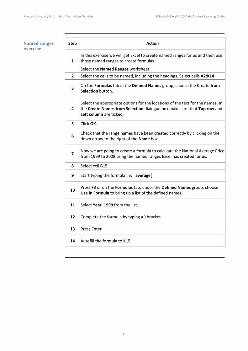
Named ranges exercise

Step Action

1 In this exercise we will get Excel to create named ranges for us and then use those named ranges to create formulas

Select the Named Ranges worksheet.

2 Select the cells to be named, including the headings. Select cells A2:K14.

3

On the Formulas tab in the Defined Names group, choose the Create from Selection button.

4 Select the appropriate options for the locations of the text for the names. In the Create Names from Selection dialogue box make sure that Top row and Left column are ticked.

5 Click OK.

6

Check that the range names have been created correctly by clicking on the down arrow to the right of the Name box.

7

Now we are going to create a formula to calculate the National Average Price from 1999 to 2008 using the named ranges Excel has created for us.

8 Select cell B15.

9 Start typing the formula i.e. =average(

10

Press F3 or on the Formulas tab, under the Defined Names group, choose Use in Formula to bring up a list of the defined names..

11 Select Year_1999 from the list.

12 Complete the formula by typing a ) bracket.

13 Press Enter.

14 Autofill the formula to K15.


12

Named ranges exercise, continued

Step Action

15 Select cell C15 and in the forrmula bar, left click Year_1999 to select it.

16

Click your right mouse button and from the shortcut menu select Pick from Drop-down list.

17 Double click on Year_2000 to select it.

18 Make sure that only Year_2000 appears in the brackets.

19 Repeat steps 15 – 18 for the rest of the years.


13

Sub Totals

Sub Totals introduction

You can use Excel 2010's Subtotals feature to subtotal data in a sorted list. To

subtotal a list, you first sort the list on the field for which you want the subtotals,

and then you designate the field that contains the values you want summed — these

don't have to be the same fields that you sorted on.

Sub totalling data Step Action

1

1 Sort the list on the field for which you want subtotals inserted.

2

On the Data tab in the Outline group click the Subtotal button.

3

Select the field for which the subtotals are to be calculated in the At Each Change in drop-down list.


14

Sub totalling data, continued

Step Action

4

Specify the type of totals you want to insert in the Use Function drop-down list. When you use the Subtotals feature, you aren't restricted to having the values in the designated field added together with the SUM function.

5 Select the check boxes for the field(s) you want to total in the Add Subtotal to list box.

6

Click OK.


15

Exercise Subtotals In this exercise we are going to create sub-totals by Location.

Step Action

1 Open the sub totalling worksheet.

Sort by Location (ascending or descending).

2 On the Data tab in the Outline group click the Subtotal button.

3

Select the field for which the subtotals are to be calculated in the At Each Change in drop-down list. In this instance it will be Location.

4 In the Use Function drop-down list ensure SUM is selected.

5 In the Add Subtotal to list box make sure, # Delivered Semester 1, # of Participants Semester 1, # Delivered Semester 2 and # of Participants Semester 2 have been selected.

6 Click OK.

7

The outline view can now be collapsed/expanded to show 1 Grand Total, 2 A total for each of the regions, 3 A breakdown per region.

Remove the sub totals by clicking into the data. On the Data tab in the Outline group click the Subtotal button. In the Subtotal dialogue box click Remove All.


16

Text Functions

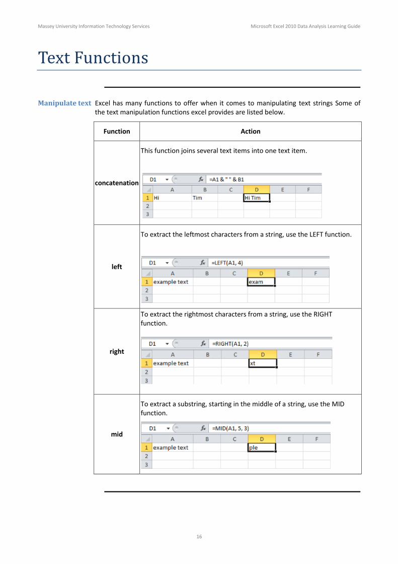
Manipulate text Excel has many functions to offer when it comes to manipulating text strings Some of the text manipulation functions excel provides are listed below.

Function Action

concatenation

This function joins several text items into one text item.

left

To extract the leftmost characters from a string, use the LEFT function.

right

To extract the rightmost characters from a string, use the RIGHT function.

mid

To extract a substring, starting in the middle of a string, use the MID function.


17

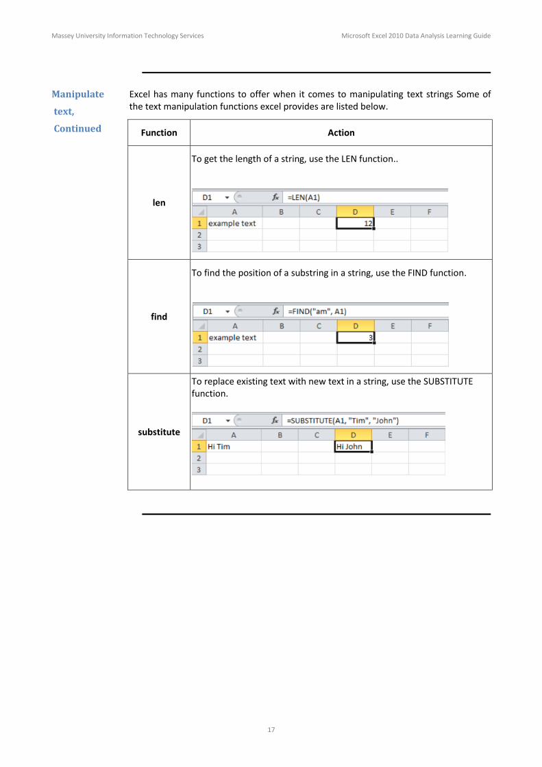
Manipulate

text,

Continued

Excel has many functions to offer when it comes to manipulating text strings Some of the text manipulation functions excel provides are listed below.

Function Action

len

To get the length of a string, use the LEN function..

find

To find the position of a substring in a string, use the FIND function.

substitute

To replace existing text with new text in a string, use the SUBSTITUTE function.


18

Exercise text manipulation

Select the text manipulation worksheet. In this practice we will extract the First Names, Last Name, Employee No and Job Title from a text string. We will then combine first names and last name into Full Name. Select the worksheet text manipulation.

Step Action

1 We first need to identify the fields in the text string that we want to extract. To do this we will need to determine the character positions of the “$”, “,” and “%” symbols, as well as the length of entire string.

2 Select cell H2.

3

Click the button on the Formula Bar to bring up the Insert Function dialog.

4

Select the Text category from the drop down arrow.

5 Select the Find function and click on OK.

6

In the function arguments dialogue box enter the information you are looking for:

Find_text: “$”

Within_text: A2

Start_num: 1

Click OK.

8 Repeat steps 3 – 7 for “,” and “%”.

10

Select cell K2, then click the button on the Formula Bar to bring up the Insert Function dialog.

11 Under the Text category select the LEN function.

12 Select cell A2 and then click on OK.


19

Exercise text manipulation, continued

Step Action

13 Now we can extract the person’s employee number using the left function.

14 Select cell B2.

15

Use the Insert Function button and select the left function from the Text group.,

16 Select A3 for the Text field.

17

For the Num_chars field enter H2 – 1. (we don’t want to include the $ symbol in our extracted string). Click OK.

18 In order to extract the Last Name field we will use the mid function.

19 Click into cell C2.

20

Use the Insert Function button and select the mid function from the Text group

21

Enter the following values for each of the arguments:

22

Perform the same process above using the mid function to extract the persons First Name.


20

Exercise text manipulation, continued

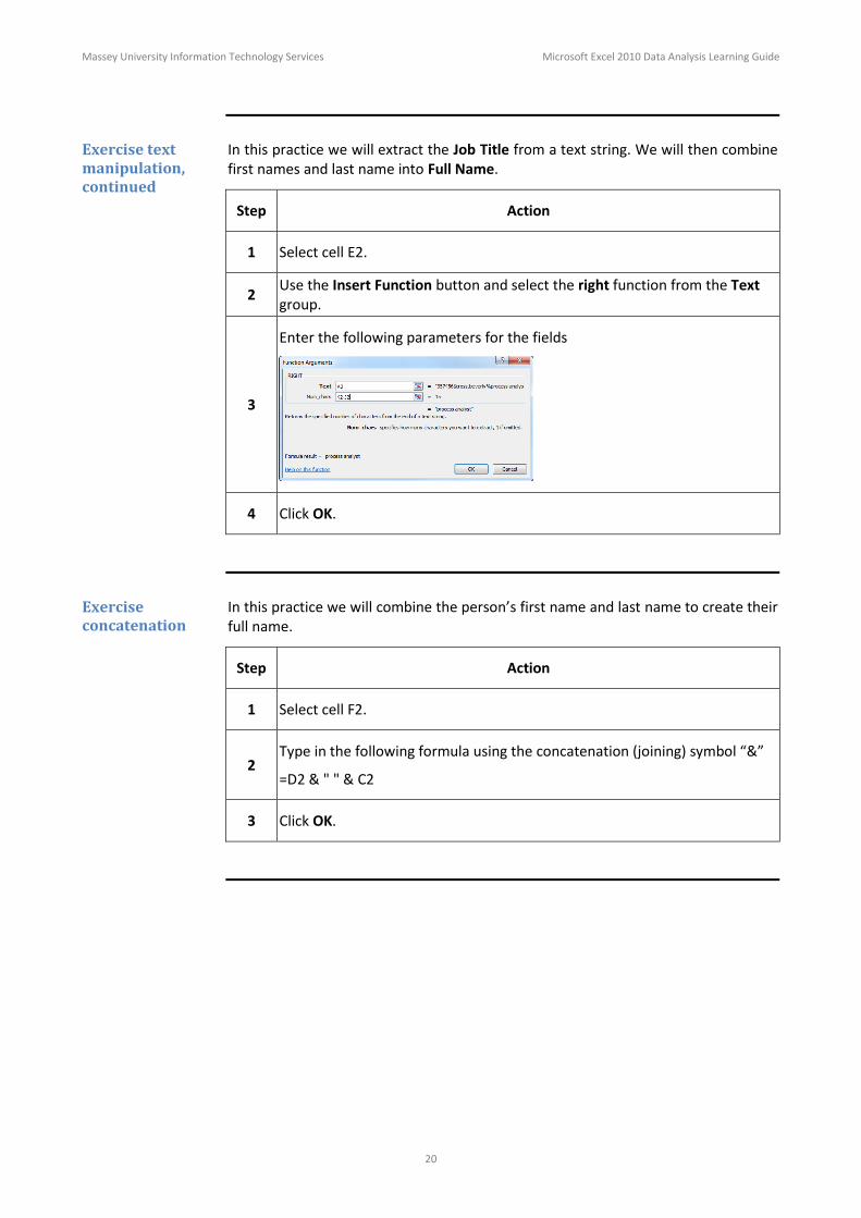
In this practice we will extract the Job Title from a text string. We will then combine first names and last name into Full Name.

Step Action

1 Select cell E2.

2

Use the Insert Function button and select the right function from the Text group.

3

Enter the following parameters for the fields

4 Click OK.

Exercise concatenation

In this practice we will combine the person’s first name and last name to create their full name.

Step Action

1 Select cell F2.

2 Type in the following formula using the concatenation (joining) symbol “&”

=D2 & " " & C2

3 Click OK.


21

Data Tables

Introduction Data tables help you explore a set of possible outcomes. When you use data tables, you are doing what-if analysis. What-if analysis is the process of changing the values in cells to see how those changes will affect the outcome of formulas on the worksheet. For example, you can use a data table to vary the interest rate and term length that are used in a loan to determine possible monthly payment amounts.

One-variable data table

If you want to see how different values of one variable in one or more formulas will

change the results of those formulas. For example, you can use a one-variable data

table to see how different interest rates affect a monthly mortgage payment by

using the PMT function. You enter the variable values in one column or row, and the

outcomes are displayed in an adjacent column or row. You can have multiple

formulas across the top row one (1) or down column A (2)

Step Action

1

A one-variable data table has input values that are listed either down a column (1 - column-oriented) or across a row (2 - row-oriented). Formulas that are used in a one-variable data table must refer to only one input cell.

In the following illustration, cells D2 (column input cell) or A8 (row input cell) contains the payment formula, =PMT(B3/12,B4,-B5), which refers to the input cell B3.

Type the list of values that you want to substitute in the input cell either down one column (1) or across one row (2).


22

One variable data table, continued

Step Action

2

Do one of the following:

If the data table is column-oriented (your variable values are in a column), type the formula in the cell one row above and one cell to the right of the column of values. Number 1in the illustration above is column-oriented.

If the data table is row-oriented (your variable values are in a row), type the formula in the cell one column to the left of the first value and one cell below the row of values. Number 2 in the illustration above is column-oriented.

3 Select the range of cells that contains the formulas and values that you want to substitute. If you are using layout 1 then, this range is C2:D5. If you are using layout 2 then this range is A7:D8.

4

On the Data tab, in the Data Tools group, click What-If Analysis, and then

click Data Table.

5

Do one of the following:

If the data table is column-oriented, type the cell reference for the

input cell in the Column input cell box. Using the example shown in

the first illustration, the input cell is B3.

If the data table is row-oriented, type the cell reference for the input

cell in the Row input cell box.

javascript:AppendPopup(this,'452225644_3')


23

Two variable data table

This allows for changing values for two variables (column A and row 1 in the example

below), but only has one formula (cell A1 in the example below).

Cell A1 contains the formula for the Data Table, range A2:A4 contains the first input variable, range B1:D1 contains the second input variables, and range A1:D4 is the Data Table range.

Enter the formula for the Data Table.

Using a two variable data table

Step Action

1 Select the Data Table Range (A1:D4)

2

On the Data tab, in the Data Tools group click the dropdown arrow next to

What-If Analysis and select Data Table.

3

Enter or select the Row Input Cell (for two-input tables only): This is the top

row values that we want substituted for the corresponding cell

reference/value the data table formula uses. Select the cell the formula uses

and the data table will substitute that value with those in the top row of the

table

4

Enter or select the Column Input Cell: This is the left column values that we

want substituted for the corresponding cell reference/value the data table

formula uses. Select the cell the formula uses and the data table will

substitute that value with those in the left column of the table.

5 Select OK.


24

Exercise – One input table

Step Action

1 Open the Data Tables workbook and select the one variable table worksheet.

2 Column E contains the values to be substituted for the interest rate used in the data table formula. The formula is in cell C10 and the interest rate it uses is in cell C7.

3 Select E3:F10 as the data table range.

4

On the Data tab, in the Data Tools group, select the drop down arrow to the right of What-If Analysis and then choose Data Table.

5 Select C7 as the column input cell and click OK.

6

Change the purchase price in cell C3 and some of the interest rates in column E and observe the recalculations.

Exercise – Two input table

1 Switch to the two variable table worksheet.

2 Select E3:I10 as the data table range.

3

On the Data tab, in the Data Tools group, select the drop down arrow to the right of What-If Analysis and then choose Data Table.

4 Select C8 (yrs.) as the Row input cell.

5 Select C7 (int. rate) as the Column input cell.

6 Click OK.

7

Change some of the years in row 3 and interest rates in column E and notice the changes.


25

Data Form

Introduction Data forms enables user to create a form for entering data. The Data Input Form feature lets you fill all the cells’ values of a single record quickly. With this feature, you no longer need to move to the required cell in the spreadsheet manually and enter the data. It lets you move through the entered data using the next and previous buttons. You can easily edit the data, delete a record and create a new record from within the data input form dialog box.

Add Form button Follow the steps below to add the Form button to the Quick Access Toolbar.

Step Action

1

Open the Excel Options window by clicking the File tab > Options. Select the Quick Access Toolbar in the left hand panel.

Click the drop down arrow to the right of Choose commands from and select All Commands.

Select the Form button and click Add to add it to the Quick Access Toolbar.

Click OK to close the window.


26

Using data forms Follow the steps below to use a Data Form:

Step Action

1

Click in a new record on a worksheet that you wish to populate using a data form. (An example worksheet is shown below).

2 Click the Form button on the Quick Access Toolbar.

The Form Window The Forms data tools are described below:

Step Action

1

The Find Prev and Find Next buttons - these allow you to scroll forward and back through the database one record at a time.

The Delete button - this is used to delete records from the database.

The Restore button - This button can be used to undo changes to a record that is being edited.

The Criteria button allows you to search the database for records based on specific criteria, such as name, age, or program.


27

Exercise – Data Forms

In this exercise we are going to use a data form to: find a record, modify it and then

delete it.

Step Action

1 Select the Data Forms worksheet. Click any cell in the data base.

2 Click on the form button that you have added to the quick access toolbar

(see step1 at the beginning of the topic).

3

Click on the Criteria button to enter search criteria.

4 In the Data Forms dialogue box type logan into the Name field and select

Find Next.

5 Once the record has been found change the department from Legal to

Salary and Finance.

6 Click on the New button. Enter any details for the new record. Click Close.

7 Check that your records have been modified and added in the database.

8

Click into the database and select the Form tool from the Quick Access

Toolbar again

9 Find the record that has IL as the State/Province/Country.

10

Click the Delete button. A message box will display saying Displayed record

will be permanently deleted. Click OK

11 Close the form dialogue box and check that the record has been deleted.


28

Consolidation

Introduction This feature allows data from multiple ranges on multiple workbooks to be

summarized on to one spreadsheet. The default consolidation uses the SUM

function. However, other functions such as AVERAGE, MAX, and MIN, are also

available.

Up to 255 source areas can be consolidated, as a once off event or linked to the

source data for immediate update.

Consolidate Multiple Ranges

Step Action

1 Select the destination cell for the consolidation.

2

On the Data tab in the Data Tools group click the Consolidate button.

3

Select the range of data (including top row and left column headings) from the first source file, and then click on Add.

Repeat for all other source files.

4

In the Use labels in box click on Top row and/or Left column. If you do not check these Excel will match the row numbers of each source file. This will summarize data incorrectly if one or more source files have more rows than the others

5 To link the summarized data to the source files, click on Create Links To

source data. This will automatically create all links.

6 Select OK.


29

Exercise consolidation

Step Action

1 Create a new worksheet. Call the new worksheet Consolidation.

2 Select cell A1 in the Consolidation worksheet.

3 On the Data tab, under the Data Tools group, choose Consolidate.

4 For the first reference select the Week1 worksheet.

5 Select cells A4:G27 and then click on Add.

6 Repeat steps 4 and 5 above for the worksheets Week2, Week3 and Week4.

7 Click on Top row and Left column in the Use labels in box.

8 Click OK.


30

Formula Auditing

Formula auditing The Formula Auditing Tool allows you to track down cells that are causing Excel errors to be displayed. By tracing the relationships between the formulas in the cells you can test formulas to see which cells, called direct precedents, directly feed the formulas, and which cells, called dependents, depend on the results of the formulas. Excel also lets you visually backtrack to the potential sources of an error value in the formula of a particular cell.

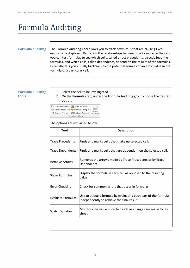
Formula auditing tools

1. Select the cell to be investigated 2. On the Formulas tab, under the Formula Auditing group choose the desired

option.

The options are explained below:

Tool Description

Trace Precedents Finds and marks cells that make up selected cell.

Trace Dependents Finds and marks cells that are dependent on the selected cell.

Remove Arrows

Removes the arrows made by Trace Precedents or by Trace Dependents.

Show Formulas

Display the formula in each cell as opposed to the resulting value.

Error Checking Check for common errors that occur in formulas.

Evaluate Formulas

Use to debug a formula by evaluating each part of the formula independently to achieve the final result.

Watch Window

Monitors the value of certain cells as changes are made to the sheet.


31

Comments A comment can be identified in a worksheet by a red triangle marking in the top

corner of a cell. To add a new comment follow the steps below

Step Action

1

On the Review tab, in the Comments group, click on the New Comment button.

2 Type the comments.

Edit or delete comments

A comment can be identified in a worksheet by a red triangle marking in the top

corner of a cell. To add a new comment follow the steps below

Step Action

1

On the Review tab, in the Comments group, click on either the Edit Comment button or the Delete button.


32

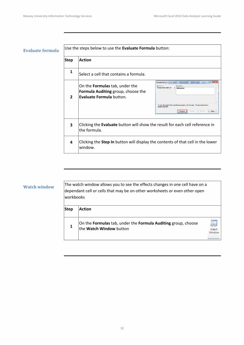
Evaluate formula Use the steps below to use the Evaluate Formula button:

Step Action

1 Select a cell that contains a formula.

2

On the Formulas tab, under the Formula Auditing group, choose the Evaluate Formula button.

3 Clicking the Evaluate button will show the result for each cell reference in the formula.

4 Clicking the Step In button will display the contents of that cell in the lower

window.

Watch window The watch window allows you to see the effects changes in one cell have on a

dependant cell or cells that may be on other worksheets or even other open

workbooks

Step Action

1 On the Formulas tab, under the Formula Auditing group, choose the Watch Window button


33

Goal Seek

Goal seek introduction

If you know the result that you want from a formula, but you are not sure what input

values the formula requires to get that result, you can use the Goal Seek feature. For

example, if you were considering purchasing a new car and knew the maximum

monthly payment you could make, it would be possible to use “Goal Seek” to

determine what size loan you could afford. You work backwards from an answer to

determine the input values needed to achieve that answer.

Using goal seek Step Action

1 On the Data tab, in the Data Tools group, click the arrow next to What-If

Analysis and select Goal Seek.

2

Set cell – Select the cell that will show the target value. This cell must contain a formula. To value – Enter the target amount. By changing cell – Select the cell that will show the required value to achieve the target value specified. This cell must not contain a formula.


34

Exercise Goal Seek In this practice we will see what effect two different revenues and two different interest rates have on our cash flow

Step Action

1 Select the Loan worksheet.

2

Use Goal Seek to calculate the maximum loan you can afford. (i.e. how much could you afford to pay back per month for 15 years at 7.02% interest rate?).


35

Group and Outline Data

Group and outline introduction

An outline that lets you hide or show levels of detail. It lets you display only the rows

or columns that provide summaries for each group of data. Outline looks for

formulas and groups together the columns and/or rows before those formula.

Summary columns should be to the left or right of the details data, and summary

rows should be either below or above the detail data. Summary columns or rows

must not be mixed with the detail data.

Auto Outline

Auto Outline will outline all sets of data on the active worksheet

Step Action

1

On the Data tab in the Outline group, choose Auto Outline.

2

The outline can be collapsed or expanded by clicking the + or – sign. The amount of detail displayed can also be chosen by clicking on the appropriate outline numbers. (e.g. 1, 2 or 3) with outline 3 showing the most detail.

3 To clear all outlines on the active worksheet, on the Data tab in the Outline

group, select the arrow below Ungroup and Clear Outline


36

Group If you want to control how groups are determined, you can manually create groups

and outlines.

Step Action

1

On the worksheet, select the detail data level for rows or columns.

2

On the Data tab in the Outline group, click the arrow below Group and select Group.

3

The Group dialogue box will display and depending on your selected data, choose if you want to group the selection by rows or columns.

4 To clear all outlines on the active worksheet, on the Data tab in the Outline group, select the arrow below Ungroup and Clear Outline.


37

Exercise Auto Outline

Step Action

1 Open the Group & Outline worksheet.

2 On the Data tab under the Outline group, choose the Group arrow and then Auto Outline.

3 Experiment with the outline buttons on the margins of the sheet.

Exercise Manual Outline

Step Action

In this exercise we will manually create groupings.

1 Select columns D to G.

2 On the Data tab, under the Outline group, choose the Group button.

3 Select rows 5 to 25

4 On the Data tab, under the Outline group, choose the Group button.

5

On the Data tab, under the Outline group, choose Ungroup and choose Clear Outline

6 Save.


38

Scenarios

Introduction A scenario is a set of values that Excel saves and can substitute automatically in cells

on a worksheet. You can create and save different groups of values on a worksheet

and then switch to any of these new scenarios to view different results.

When using Goal Seek you cannot easily compare several different outcomes.

Scenarios are used to show various outcomes based on applying different

conditions.

Creating Scenarios Step Action

1 Select the cell that has the value that you want to change.

2

On the Data tab, under the Data Tools group, choose the What-If Analysis button and choose Scenario Manager.

Click Add.

3

Enter a Name for the first scenario, for example, Low Revenue.

4 Ensure the Changing Cell is the same as the one selected in step 1. Above

and then click OK.

5 Enter the value for the Changing Cell.

6 To enter additional scenarios, click Add or click OK to return to the Scenario

Manager dialog box..


39

Editing Scenarios Step Action

1 On the Data tab, under the Data Tools group, choose the What-If Analysis button and choose Scenario Manager

2 Select the Scenario Name you want to edit, and then click Edit.

Creating Scenario Reports

Step Action

1 On the Data tab, under the Data Tools group, choose the What-If Analysis button and choose Scenario Manager

2 Click on Summary.

3 Choose the Report Type required and the Result Cells then click OK


40

Using Scenario Manager

Follow the example below to use Scenario Manager

Step Action

1

Open the Sales Forecast worksheet.

The example uses three scenarios based on the following sets of values for

the three changing cells: (COGS = Cost of Goods Sold)

Most Likely, where the Sales_Growth percentage is 5%, COGS is 20%, and Expenses is 25%

Best Case, where the Sales_Growth percentage is 8%, COGS is 18%, and Expenses is 20%

Worst Case, where the Sales_Growth percentage is 2%, COGS is 25%, and Expenses is 35%.

Select cells H3 (Sales), H4 (Cost of Goods Sold) and H6 (Expenses).

2 On the Data tab in the Data Tools group, choose What-If-Analysis and then

Scenario Manager.

3

To create a scenario, click the Add button.

4 Type the name of the scenario (Most Likely, in this example) in the Scenario Name text box, specify the Changing Cells (if they weren't previously selected), and click OK.


41

Scenario Manager, continued

Step Action

5

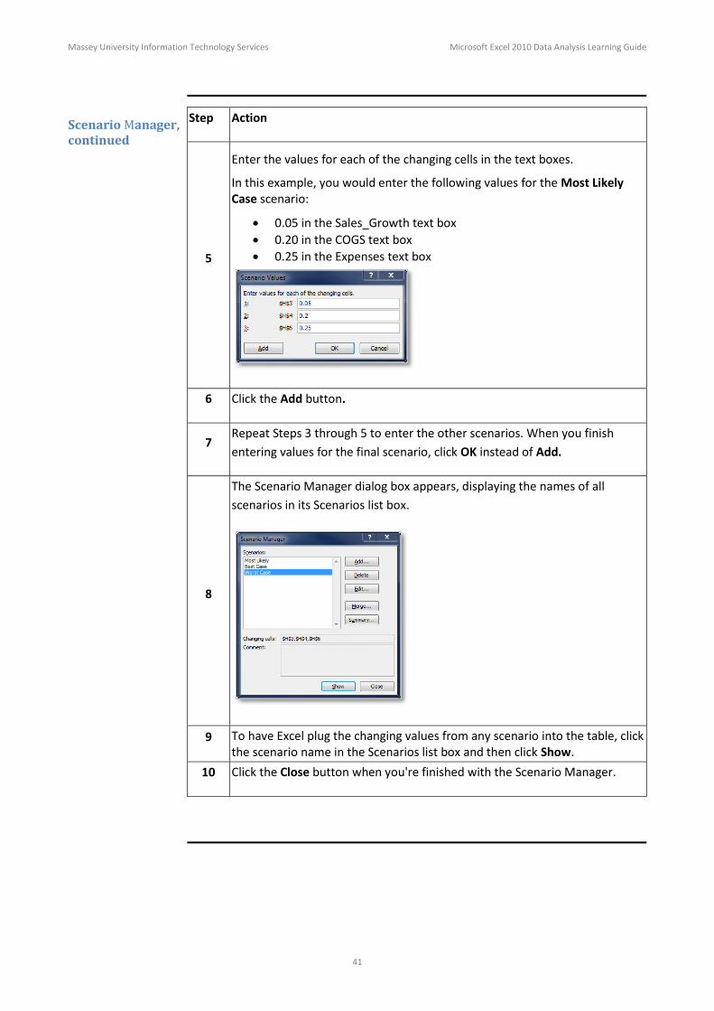
Enter the values for each of the changing cells in the text boxes.

In this example, you would enter the following values for the Most Likely Case scenario:

0.05 in the Sales_Growth text box

0.20 in the COGS text box

0.25 in the Expenses text box

6 Click the Add button.

7 Repeat Steps 3 through 5 to enter the other scenarios. When you finish

entering values for the final scenario, click OK instead of Add.

8

The Scenario Manager dialog box appears, displaying the names of all

scenarios in its Scenarios list box.

9 To have Excel plug the changing values from any scenario into the table, click the scenario name in the Scenarios list box and then click Show.

10 Click the Close button when you're finished with the Scenario Manager.


42

Exercise Scenarios In this practice we will see what effect two different revenues and two different interest rates have on our cash flow

Step Action

1 Open the sheet Scenario in the workbook What If Analysis.

2 Select cells E4 & H3.

3

On the Data tab, under the Data Tools group, choose the What-If Analysis button and choose Scenario Manager.

4 Click on Add.

5 Name this scenario Standard Revenue Standard Interest. Click OK.

6 Ensure that the Changing Cells are E4, H3. Click OK.

7

The values in this next dialog should have set themselves to the current value of cell E4 and H3, which is what we want.

Click Add. We shall add another scenario.

8 Name this Scenario Low Revenue Normal Interest. Click OK.

9 Enter 375000 as the value for E4 and leave the value for H3 as 0.825

10 Click Add. Name the third scenario Normal Revenue Low Interest.

11 Click OK. Leave E4 at 500000 and enter 0.05 for H3.

12 Click Add. Name the fourth scenario Low Revenue Low Interest.

13 Click OK. Enter 375000 as the value for E4 and 0.05 for H3.

14 Click OK.

15

Select the different scenarios and click Show to view the changes on the worksheet.

16

For a summary of the different scenarios, select cell E21 and then click on the Summary button.


43

Lookup - Vlookup

Introduction Excel contains several lookup functions, which can go to a table of data and bring

back items of information you ask for. For example, you would use this function if

you entered a product code into cell A1 and wanted Excel to immediately display the

description and price of that product in cells B1 and C1.

The VLOOKUP function searches for a value in the leftmost column of a table and

returns a value in the same row from a column you specify in the table. The

HLOOKUP does the same sort of thing except that it searches across a row and

returns values from the same column.

Using VLookup The format of a VLOOKUP is as follows:

=VLOOKUP(lookup value, table array, col number, range lookup).

or in simpler terms:

=VLOOKUP(What to look up, Where to find it, Which Column Number to return , No error if not found? (True).

Argument Name Description

Lookup Value

Data that is to be looked up. Exists in the first column of the

Table Array.

Table Array (or Range

to look up)

The range that contains the Lookup Value and associated

details.

Column Number

Column number of the cell that has the answer to be

displayed.

Range Lookup TRUE or FALSE. Use FALSE if you want an error message if

the lookup value is not found.

Note: If the range lookup argument is not used it defaults to TRUE. The first column in the table array must be sorted in ascending order


44

More Information on Vlookup

The column number argument is a number. This refers to the column the data you want to retrieve is in. Columns in the table array are numbered from left to right starting from 1. Ignore column letters such as A, B, C. If your database is contained in the area D10:I30 and column I (the fiveth column) contains the items you want, then specify 5 as column number.

Warning: A VLOOKUP cannot look to the left of the lookup value column.

Place the active cell where you want the value to be returned and enter the VLOOKUP formula based on the details given above.

Tip:

1) Name your table array.

2) Check your column number value before you start building the formula


45

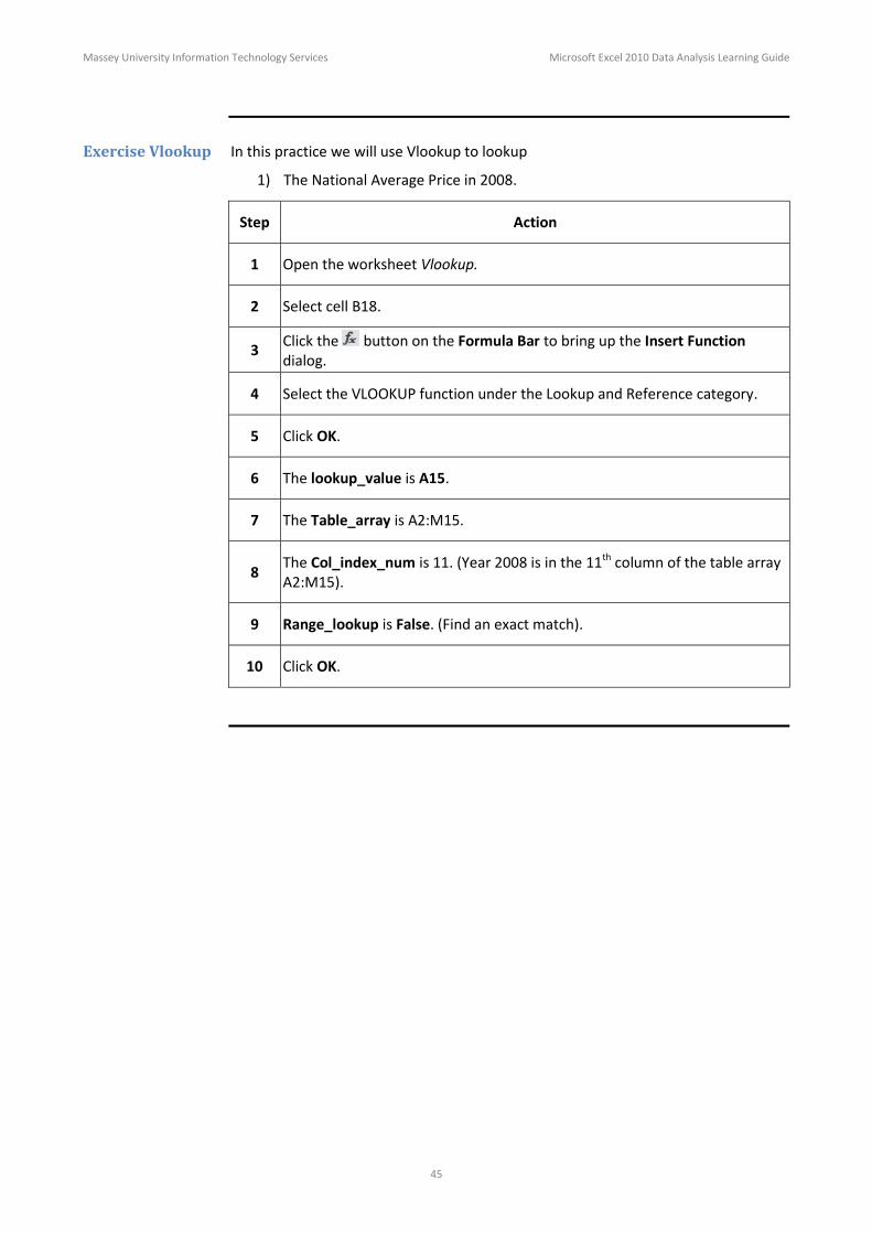
Exercise Vlookup In this practice we will use Vlookup to lookup

1) The National Average Price in 2008.

Step Action

1 Open the worksheet Vlookup.

2 Select cell B18.

3


4 Select the VLOOKUP function under the Lookup and Reference category.

5 Click OK.

6 The lookup_value is A15.

7 The Table_array is A2:M15.

8

The Col_index_num is 11. (Year 2008 is in the 11th column of the table array A2:M15).

9 Range_lookup is False. (Find an exact match).

10 Click OK.


46

Exercise 2 Vlookup In this practice we will use Vlookup to lookup the median price in 2002 in Taranaki

Step Action

1 Open the sheet Vlookup in the workbook What If Analysis.

2 Select cell B19.

3


4 Select the VLOOKUP function under the Lookup and Reference category.

5 Click OK.

6 The lookup value is A13.

7 The Table_array is A2:M15.

The Col_index_num is 5. (Year 2002 is in the 5th column of the table array A2:M15).

Range_lookup is False. (find an exact match).

Click OK.

INFORM A TION TECHNOLOGY SERV ICES

Documents

Transcript of INFORM A TION TECHNOLOGY SERV ICES