Influence of viscoelasticity on drop deformation andorientation in shear flow, part 1: Stationary statesVerhulst, K.; Cardinaels, R.M.; Moldenaers, P.; Renardy, Y.; Afkhami, S.

Published in:Journal of Non-Newtonian Fluid Mechanics

DOI:10.1016/j.jnnfm.2008.06.007

Published: 01/01/2009

Document VersionAccepted manuscript including changes made at the peer-review stage

Please check the document version of this publication:

• A submitted manuscript is the author's version of the article upon submission and before peer-review. There can be important differencesbetween the submitted version and the official published version of record. People interested in the research are advised to contact theauthor for the final version of the publication, or visit the DOI to the publisher's website.• The final author version and the galley proof are versions of the publication after peer review.• The final published version features the final layout of the paper including the volume, issue and page numbers.

Link to publication

Citation for published version (APA):Verhulst, K., Cardinaels, R. M., Moldenaers, P., Renardy, Y., & Afkhami, S. (2009). Influence of viscoelasticityon drop deformation and orientation in shear flow, part 1: Stationary states. Journal of Non-Newtonian FluidMechanics, 156(1-2), 29-43. DOI: 10.1016/j.jnnfm.2008.06.007

General rightsCopyright and moral rights for the publications made accessible in the public portal are retained by the authors and/or other copyright ownersand it is a condition of accessing publications that users recognise and abide by the legal requirements associated with these rights.

• Users may download and print one copy of any publication from the public portal for the purpose of private study or research. • You may not further distribute the material or use it for any profit-making activity or commercial gain • You may freely distribute the URL identifying the publication in the public portal ?

Take down policyIf you believe that this document breaches copyright please contact us providing details, and we will remove access to the work immediatelyand investigate your claim.

Download date: 16. Sep. 2018

Influence of viscoelasticity on drop deformation and orientation in shear flow

Part 1. Stationary states

K. Verhulst, R. Cardinaels, P. Moldenaers

Lab for Applied Rheology and Polymer Processing

Department of Chemical Engineering

KU Leuven

Willem de Croylaan 46, Box 2423, B-3001 Leuven, Belgium

Paula.Moldenaers@cit.kuleuven.be

Y. Renardy, S. Afkhami

Department of Mathematics and ICAM

Virginia Polytechnic Institute and State University

460 McBryde Hall, Blackburg , VA24061-0123, USA

Renardyy@aol.com

Final accepted draft

Cite as: K. Verhulst, R. Cardinaels, P. Moldenaers, Y. Renardy, S. Afkhami, J. Non-Newt. Fluid

Mech., 156(1-2), pp. 29-43 (2009)

The original publication is available at:

http://www.sciencedirect.com/science/article/pii/S037702570800116X

Influence of viscoelasticity on drop

deformation and orientation in shear flow

Part 1: Stationary states

Kristof Verhulst a Ruth Cardinaels a Paula Moldenaers a

aKatholieke Universiteit Leuven, Department of Chemical Engineering, W. deCroylaan 46 - B 3001 Heverlee (Leuven), Belgium

Yuriko Renardy b Shahriar Afkhami b

bDepartment of Mathematics and ICAM, 460 McBryde Hall, Virginia PolytechnicInstitute and State University, Blackburg VA 24061-0123, USA

Abstract

The influence of matrix and droplet viscoelasticity on the steady deformation andorientation of a single droplet subjected to simple shear is investigated micro-scopically. Experimental data are obtained in the velocity-vorticity and velocity-velocity gradient plane. A constant viscosity Boger fluid is used, as well as a shear-thinning viscoelastic fluid. These materials are described by means of an Oldroyd-B,Giesekus, Ellis, or multi-mode Giesekus constitutive equation. The drop-to-matrixviscosity ratio is 1.5. The numerical simulations in 3D are performed with a volume-of-fluid algorithm and focus on capillary numbers 0.15 and 0.35. In the case of aviscoelastic matrix, viscoelastic stress fields, computed at varying Deborah num-bers, show maxima slightly above the drop tip at the back and below the tip at thefront. At both capillary numbers, the simulations with the Oldroyd-B constitutiveequation predict the experimentally observed phenomena that matrix viscoelasticitysignificantly suppresses droplet deformation and promotes droplet orientation, twoeffects that saturate at high Deborah numbers. Experimentally, this correspondsto decreasing the droplet radius with other parameters unchanged. At the highercapillary and Deborah numbers, the use of the Giesekus model with a small amountof shear-thinning dampens the stationary state deformation slightly and increasesthe angle of orientation. Droplet viscoelasticity on the other hand hardly affects thesteady droplet deformation and orientation, both experimentally and numerically,even at moderate to high capillary and Deborah numbers.

Key words: drop deformation, Oldroyd-B model, volume-of-fluid method, blendmorphology, viscoelasticity

Preprint submitted to Elsevier 15 February 2008

1 Introduction

Dilute polymeric blends commonly form a droplet-matrix interface [1, 2]. Thefinal material properties are significantly influenced by the deformation, break-up and coalescence of droplets during flow. Control of these processes is there-fore essential in the development of high performance blends. The investigationof single droplet dynamics in simple shear is a contribution toward this goal.In fact, theoretical and experimental studies on the single droplet problemrecently include the effects of component viscoelasticity [3]. Perturbation the-ories for small deformation [4, 5] predict that viscoelasticity hardly affectsthe steady droplet deformation at low flow intensity. Steady droplet orienta-tion towards the (shear) flow direction is predicted to be highly promoted bymatrix viscoelasticity. The effect of droplet viscoelasticity on the orientationof the droplet is less pronounced. Several experimental studies confirm thesetrends [6, 7, 8].

The small deformation theories are modified and extended to handle largerdroplet deformations in recent phenomenological models. In the case of steadydroplet deformation, quantitative agreement is found for low to moderatedroplet deformations. At high droplet deformations, the discrepancy with ex-perimental results is more pronounced. [8, 9, 10, 11, 12, 13, 14].

In planar extensional flow [15] and uniaxial elongational flow [16], matrixelasticity promotes droplet deformation at stationary states for viscosity ra-tios (λ = drop to matrix ratio) less than or equal to one. In the case ofdroplet elasticity, the opposite is found [16, 17]. For λ > 1, experiments onplanar extensional flow with various non-Newtonian droplet systems result instationary shapes that resemble corresponding Newtonian-Newtonian systems[18]. Less attention has been given to the study of simple shear. Experimentalresults of Guido et al. [7] demonstrate that matrix viscoelasticity suppressesdroplet deformation at high flow intensities at viscosity ratios 0.1, 1 and 4.7.This result is confirmed by Verhulst et al. [8] at viscosity ratio 0.75 and isin qualitative agreement with the predictions of the phenomenological models[9, 10, 11]. On the contrary, several authors conclude the opposite, i.e. matrixelasticity enhances droplet deformation [19, 20, 21]. The numerical investi-gation of Yue et al. [22] clarifies the interaction between the various stresscomponents and pressure acting on the surface of the droplet, and explainsthe differences according to the level of matrix elasticity. In addition, Verhulstet al. [8] demonstrate that similar materials, studied at moderate to high shearrates, can yield different steady droplet deformations under the same exper-imental conditions; i.e. when the same dimensionless parameters (borrowed

1 Corresponding author:Email address: renardyy@aol.com Y. Renardy

2

from small deformation theory) are studied for different materials.

Experimental studies on the deformation of a viscoelastic droplet in a New-tonian matrix have only been performed at a viscosity ratio of one in thepapers of Lerdwijitjarud et al. [23, 24] and Sibillo et al. [13]. In the latter, theexperimental results are compared with a model equation. Numerical simula-tions are conducted in [25] for an Oldroyd-B droplet in a Newtonian matrixunder simple shear. The drop is found to deform less as the Deborah numberincreases, while at high capillary numbers, the deformation increases with in-creasing Deborah number. A first-order ordinary differential equation is usedas a phenomenological model [25]. It describes an overdamped system, in whichthe viscous stretching force is proportional to the shear rate, a damping termis proportional to viscosity, and a restoring force is proportional to the firstnormal stress difference. The latter creates an elastic force which acts to even-tually decrease deformation, but it predicts greater decrease than observed inthe numerical results. Moreover, the model can not predict the critical curvein the Ca vs. λ parameters for the Stokes regime, nor the transient over-shoot which results from strong initial conditions [26], or predict results fora Newtonian drop in a viscoelastic matrix. The suppression of deformationwith increasing drop elasticity is also noted in the theoretical and numericalstudies of [9, 22, 27, 28].

In this paper, the influence of both matrix and droplet viscoelasticity on thesteady deformation and orientation of a single droplet subjected to a ho-mogeneous shear flow is investigated at a viscosity ratio of 1.5. The studyis performed for a broad range of the relevant dimensionless parameters,which allows the examination of the dependence on matrix elasticity in 3Dat high Deborah numbers. The 2D study of [22] finds a numerically smallnon-monotonic dependence of stationary state deformation on the matrix Deb-orah number, which is not noticeable in 3D for the specific parameters of thisstudy. Throughout this paper, the experimental results are compared withthree-dimensional simulations performed with a volume-of-fluid algorithm forviscoelastic liquid-liquid systems.

2 Numerical simulations

The governing equations are as follows. The liquids are density-matched. Foreach liquid, the solvent viscosity is denoted ηs, polymeric viscosity ηp, totalviscosity η = ηs + ηp, relaxation time τ , shear rate γ̇, and the initial elasticmodulus G(0) = ηp/τ . Additional subscripts ‘d’ and ‘m’ denote the dropand matrix liquids. The governing equations include incompressibility andmomentum transport:

3

∇ · u= 0,

ρ(∂u

∂t+ u · ∇u) =∇ · T −∇p + ∇ · (ηs(∇u + (∇u)T )) + F, (1)

where T denotes the extra stress tensor. The total stress tensor is τ = −pI +T + ηs[∇u + (∇u)T ]. Each liquid is identified with a color function,

C(x, t) ={

0 in the matrix liquid1 in the drop

(2)

which advects with the flow. The position of the interface is given by thediscontinuities in the color function. The interfacial tension force is formulatedas a body force

F = Γκ̃nδS, κ̃ = −∇ · n, (3)

where Γ denotes the surface tension, n the normal to the interface, δS thedelta-function at the interface, and κ̃ the curvature. In (3), n = ∇C/|∇C|,δS = |∇C|.

The drop and matrix liquids are governed by the Giesekus constitutive equa-tions, which has had reasonable success in comparisons of two-layer channelflow with actual data [29]. One feature that distinguishes the Giesekus modelfrom others is the non-zero second normal stress difference N2. This is rele-vant to the flow of two immiscible liquids because it has been shown that adiscontinuity in N2 affects interfacial stability [30]. In one limit, the Giesekusmodel reduces to the simpler Oldroyd-B constitutive equation. The experi-mental data which are addressed in this paper are as a first approximation,Oldroyd-B liquids [8]. However, the Oldroyd-B model is a difficult one to im-plement because it overpredicts the growth of stresses at large deformationrates and lead to numerical instability. The Giesekus constitutive equation is

τ(∂T

∂t+ (u · ∇)T − (∇u)T − T(∇u)T

)+ T + τκT2

= τG(0)(∇u + (∇u)T ). (4)

The dimensionless parameters are the viscosity ratio (based on total viscosi-ties) λ = ηd

ηm, a capillary number Ca = R0γ̇ηm

Γ, a Weissenberg number per fluid

We = γ̇τ , and retardation parameter per fluid β = ηs

η. A Reynolds number

based on the matrix liquid Re =ργ̇R2

0

ηmis in the range .01 to .05, chosen small

so that inertia is negligible.

Alternatively, let Ψ1 denote the first normal stress coefficient, equivalent to2ηpτ , and define the Deborah number by

4

D̃e =Ψ1Γ

2R0η2; (5)

i.e., D̃ed = (1 − βd)We/(λCa), and D̃em = (1 − βm)We/Ca. Numerical andexperimental results in later sections are presented in terms of the Deborahnumbers, and dimensionless capillary time

tΓ

ηmR0

=tγ̇

Ca, (6)

hereinafter denoted t̂. The rescaled Giesekus parameter

τκG(0) (7)

is relabeled κ̂. The physically viable range is 0 ≤ κ̂ < 0.5 [30]. The Oldroyd-Bmodel is κ̂ = 0.

The governing equations are discretized with the volume-of-fluid (VOF) methodgiven in Ref. [26]. The interfacial tension force (3) is approximated by eitherthe continuum surface force formulation (CSF) or the parabolic representa-tion of the interface for the surface tension force (PROST). The reader isreferred to Refs. [31, 32, 28] for these algorithms. Both VOF-PROST andVOF-CSF codes are parallelized with OpenMP. The efficiency of the paral-lelization for the Newtonian part of the code is discussed in [33]; the viscoelas-tic part has analogous properties. A typical computation presented in thispaper is ∆x = R0/16, ∆t̂ = 0.00005/Ca, Lx = 16R0, Ly = 8R0, Lz = 8R0,for which one timestep takes 1.2 seconds with 64 processors on the SGI Altix3700 supercluster at Virginia Tech. A simulation from dimensionless capillarytime 0 to 11, with 64 nodes takes roughly 25 hours.

2.1 Boundary conditions

The computational domain is denoted 0 ≤ x ≤ Lx, 0 ≤ y ≤ Ly, 0 ≤ z ≤ Lz.The boundaries at z = 0, Lz are walls which move with speeds ±U0. Thisresults in the velocity field (U(z), 0, 0) in the absence of the drop, whereU(z) = U0(2z − Lz)/Lz. The shear rate is γ̇ = U ′(z) = 2U0/Lz. Spatial pe-riodicity is imposed in the x and y directions, at x = 0, Lx and y = 0, Ly,respectively. Additional boundary conditions are not needed for the extrastress components. For computational efficiency, Lx, Ly and Lz are chosento minimize the effect of neighboring drops and that of the walls. Typically,the distance between the walls is eight times the drop radius, as is the span-wise period, and the period in the flow direction is chosen dependent on dropextension. In these and prior (Newtonian) simulations, the influence of the

5

boundaries is negligible under these circumstances. Experimental results onthe effect of confinement are consistent with this [34].

2.2 Initial conditions

The drop is initially spherical with radius R0. The top and bottom wallsare impulsively set into motion from rest. This requires that the viscoelasticstress tensor and velocity are initially zero. Since the velocity field is essen-tially governed by a parabolic PDE close to Stokes flow, the velocity adjustsimmediately to simple shear so that whether the initial velocity field is zeroor simple shear makes no difference in the numerical simulations. The initialviscoelastic stress values do, on the other hand, influence drop deformation.For example, if the drop were placed in a pre-existing shear flow, the initialviscoelastic stress is equal to the values which would prevail in the correspond-ing simple shear flow with the given shear rate. Figure 4 of [26] shows thata drop placed in an already established flow immediately experiences a largeviscoelastic stress and the deformation may overshoot. On the other hand, ifthe matrix fluid is viscoelastic with zero initial viscoelastic stress, then evenwith an established velocity field, it starts out with lower viscous stress dueto the absence of polymer viscosity. This lowers the magnitude of stress in thematrix fluid, which pulls the drop more gently.

2.3 Drop diagnostics

We report the drop diagnostics with the same notation as in [8, 35]. The slicethrough the center in the x− z plane, or the velocity-velocity gradient plane,provides the drop length L and breadth B. The angle of inclination to the flowdirection is denoted θ. When viewed from above the drop, the slice throughthe center of the drop in the x− y plane, or the velocity-vorticity plane, givesthe drop width W and length Lp. The Taylor deformation parameters areD = (L − B)/(L + B) and Dp = (Lp − W )/(Lp + W ). The viscoelastic stressfields displayed in this paper are generated from contour values of the trace ofthe extra stress tensor, tr (T). This is directly proportional to the extensionof the polymer molecules, and is meaningful to plot from the direct numericalsimulations. This quantity is directly related to experimental measurementson stress fields with birefringence techniques. Contour values are given on thenumerical plots in order to provide a comparison among the plots.

6

0 5 10 15 20 25 30

1

1.1

1.2

1.3

1.4

1.5

1.6

1.7

1.8

1.9

2

L/2R

0

t̂

Fig. 1. Newtonian reference system with viscosity ratio 1.5 (system 4 of table 2).Experimental data (− ·−) at Ca = 0.156 (lower), 0.363 (upper) are compared withnumerical simulations with the boundary integral code of [36] (−−) and VOF-CSF(—).

2.4 Accuracy

Computational accuracy for the Oldroyd-B portion is discussed in [28] for the2D code, and in [26] for the 3D version. Figure 1 is a comparison of the exper-imental data (-.-) on the sideview length for the Newtonian reference system4 of table 2. Two numerical methods, the VOF-CSF (-) and the boundaryintegral scheme of Ref. [36], are used to provide quantitative agreement.

Tests for convergence with spatial and temporal refinements are performed todecide on optimal meshing. Table 1 shows deformation and angle of inclinationfor an Oldroyd-B drop in Newtonian matrix with the CSF formulation atCa = 0.35, D̃ed = 2.6, λ = 1.5 and Re = 0.05. The computational box isLx = 16R0, Ly = 8R0, Lz = 8R0. The results are also close for the PROSTalgorithm; since PROST is more CPU intensive, CSF is used for later results.

Figure 2 shows viscoelastic stresses computed for the vertical cross-sectionthrough the center of a Oldroyd-B drop. The first row is t̂ = 5, the secondrow is t̂ = 10 and the third is t̂ = 15. With ∆tγ̇ = 0.0001, the mesh is variedfrom ∆x = R0/8 for the first column, ∆x = R0/12 for the middle columnand R0/16 for the third column. The middle column is chosen as optimal:

7

0.75 0.8 0.85 0.9 0.95 1 1.050.35

0.4

0.45

0.5

0.55

0.6

0.15

0.2

0.25

0.3

0.35

0.4

0.45

0.5

0.55

0.75 0.8 0.85 0.9 0.95 1 1.050.35

0.4

0.45

0.5

0.55

0.6

0.15

0.2

0.25

0.3

0.35

0.4

0.45

0.5

0.55

0.75 0.8 0.85 0.9 0.95 1 1.050.35

0.4

0.45

0.5

0.55

0.6

0.15

0.2

0.25

0.3

0.35

0.4

0.45

0.5

0.55

0.75 0.8 0.85 0.9 0.95 1 1.050.35

0.4

0.45

0.5

0.55

0.6

0.15

0.2

0.25

0.3

0.35

0.4

0.45

0.5

0.55

0.75 0.8 0.85 0.9 0.95 1 1.050.35

0.4

0.45

0.5

0.55

0.6

0.15

0.2

0.25

0.3

0.35

0.4

0.45

0.5

0.55

0.75 0.8 0.85 0.9 0.95 1 1.050.35

0.4

0.45

0.5

0.55

0.6

0.15

0.2

0.25

0.3

0.35

0.4

0.45

0.5

0.55

0.75 0.8 0.85 0.9 0.95 1 1.050.35

0.4

0.45

0.5

0.55

0.6

0.15

0.2

0.25

0.3

0.35

0.4

0.45

0.5

0.55

0.75 0.8 0.85 0.9 0.95 1 1.050.35

0.4

0.45

0.5

0.55

0.6

0.15

0.2

0.25

0.3

0.35

0.4

0.45

0.5

0.55

0.75 0.8 0.85 0.9 0.95 1 1.050.35

0.4

0.45

0.5

0.55

0.6

0.15

0.2

0.25

0.3

0.35

0.4

0.45

0.5

0.55

Fig. 2. Contour plots for viscoelastic stress for a Oldroyd-B drop in Newtonianmatrix, Ca = 0.35, D̃ed = 2.6, λ = 1.5, t̂ = 5 (row 1), 10 (row 2), 15 (row 3);refinement left to right ∆x = R0/8, R0/12, R0/16.

∆x = R0/12 for Ca = 0.35, D̃ed = 2.6, λ = 1.5. The temporal mesh is alsovaried to optimize the timestep. The stresses vary steeply close to the interfaceand the contours are constructed from an interpolation of the values from thesimulations. This procedure may contribute to some inaccuracy in the shapeof the contours, and also that they cross the interface. It is clear therefore thatmesh refinement reduces these features. A sensitivity study on the Reynoldsnumber is performed at Ca = 0.35, D̃ed = 0, D̃em = 1.8, βm = 0.68, λ = 1.5,Lx = 16R0, Ly = 8R0, Lz = 8R0, ∆x = R0/12. The following produce similarresults: (i) Re = 0.05, ∆t̂ = 0.00003, (ii) Re = 0.01, ∆t̂ = 0.00003, (iii)Re = 0.05, ∆t̂ = 0.000014, all with CSF, and (iv) Re = 0.05, ∆t̂ = 0.00003with PROST. Re = 0.05 is chosen as optimal.

3 Materials and experimental methods

Table 2 lists the interfacial tension and viscosity ratio for the droplet-matrixsystems used in this study. The first two blends carry a viscoelastic droplet

8

Fig. 3. Rheological characterization of the viscoelastic fluids at a reference temper-ature of 25 ◦C. (a) PIB Boger fluid BF2. First normal stress difference: M, viscos-ity: ♦, first normal stress coefficient: ◦; Lines are the Oldroyd-B model. (b) BranchedPDMS BR16. Open symbols are dynamic data, 2G′/(ωaT )2: ◦, dynamic viscosity: ♦,2G′: M; filled symbols are steady shear data, first normal stress coefficient: •, vis-cosity: ¨, first normal stress difference: N; Lines are the Ellis model.

phase; the third blend contains a viscoelastic matrix phase; and the fourthone acts as the reference system, containing only Newtonian components.

The viscoelastic material is either a branched polydimethylsiloxane (PDMS)named BR16, or a polyisobuthylene Boger fluid (PIB) named BF2 which isdescribed in detail in [8]. Preparation of the Boger fluid requires the additionof 0.2 weight percentage of a high molecular weight rubber (Oppanol B200)to a Newtonian PIB (Infineum S1054), which acts as the non-volatile solvent.As Newtonian materials, various mixtures of linear PDMS (Rhodorsil) or PIB(Infineum or Parapol) are used in order to obtain the desired viscosity ratioof 1.5. In addition, the PDMS used as the matrix fluid is saturated with alow molecular weight polyisobuthylene (Indopol H50). This saturation stepis necessary to avoid diffusion of PIB molecules, which would lead to dropletshrinkage and a time-dependent interfacial tension [37]. The interfacial tensionin table 2 is measured with two independent methods, which both agree towithin experimental error: (i) fitting the droplet deformation at small flowintensity to the second-order theory of Greco [4] and (ii) the pendant dropmethod.

The rheology of the blend components is discussed in detail in section III.Aof Ref. [8]. Briefly, all Rhodorsil PDMS mixtures, the Parapol 1300, and theInfineum mixture are Newtonian in the results of this paper. The steady shearrheological data of the PIB Boger fluid at 25 ◦C is shown in fig. 3a. The viscos-ity and first normal stress coefficient are clearly constants. Thus, the Oldroyd-B constitutive model is appropriate to describe the steady shear rheology,where the solvent viscosity equals that of the non-volatile solvent (InfineumS1054).

9

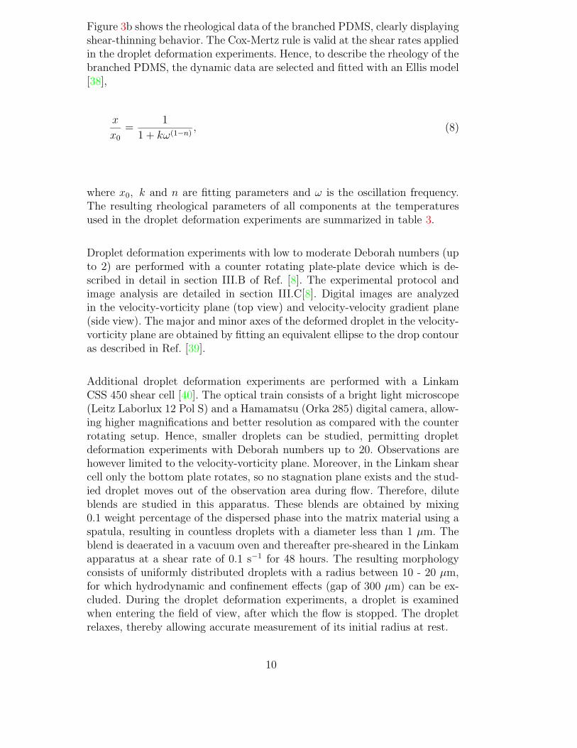
Figure 3b shows the rheological data of the branched PDMS, clearly displayingshear-thinning behavior. The Cox-Mertz rule is valid at the shear rates appliedin the droplet deformation experiments. Hence, to describe the rheology of thebranched PDMS, the dynamic data are selected and fitted with an Ellis model[38],

x

x0

=1

1 + kω(1−n), (8)

where x0, k and n are fitting parameters and ω is the oscillation frequency.The resulting rheological parameters of all components at the temperaturesused in the droplet deformation experiments are summarized in table 3.

Droplet deformation experiments with low to moderate Deborah numbers (upto 2) are performed with a counter rotating plate-plate device which is de-scribed in detail in section III.B of Ref. [8]. The experimental protocol andimage analysis are detailed in section III.C[8]. Digital images are analyzedin the velocity-vorticity plane (top view) and velocity-velocity gradient plane(side view). The major and minor axes of the deformed droplet in the velocity-vorticity plane are obtained by fitting an equivalent ellipse to the drop contouras described in Ref. [39].

Additional droplet deformation experiments are performed with a LinkamCSS 450 shear cell [40]. The optical train consists of a bright light microscope(Leitz Laborlux 12 Pol S) and a Hamamatsu (Orka 285) digital camera, allow-ing higher magnifications and better resolution as compared with the counterrotating setup. Hence, smaller droplets can be studied, permitting dropletdeformation experiments with Deborah numbers up to 20. Observations arehowever limited to the velocity-vorticity plane. Moreover, in the Linkam shearcell only the bottom plate rotates, so no stagnation plane exists and the stud-ied droplet moves out of the observation area during flow. Therefore, diluteblends are studied in this apparatus. These blends are obtained by mixing0.1 weight percentage of the dispersed phase into the matrix material using aspatula, resulting in countless droplets with a diameter less than 1 µm. Theblend is deaerated in a vacuum oven and thereafter pre-sheared in the Linkamapparatus at a shear rate of 0.1 s−1 for 48 hours. The resulting morphologyconsists of uniformly distributed droplets with a radius between 10 - 20 µm,for which hydrodynamic and confinement effects (gap of 300 µm) can be ex-cluded. During the droplet deformation experiments, a droplet is examinedwhen entering the field of view, after which the flow is stopped. The dropletrelaxes, thereby allowing accurate measurement of its initial radius at rest.

10

Fig. 4. Steady state droplet deformations and orientation. Open symbols: Bogerfluid droplet - Newtonian matrix system (System 1 of table 2) at various D̃ed; filledsymbols: Newtonian reference system.

4 Results and discussion

4.1 Boger fluid droplet system

The effects of droplet viscoelasticity on the droplet deformation and orien-tation are systematically studied over a wide range of Deborah and capillarynumbers and thus contribute to the scarce data on viscoelastic droplet systems.Figure 4 shows the stationary droplet deformations D and Dp, and orientationof a Boger fluid droplet in a Newtonian matrix (System 1, table 2). The New-tonian/Newtonian reference (System 4, table 2) is also plotted for comparison.The range of Deborah number is achieved by varying the radius of the droplet.The counter-rotating setup was used, yielding the complete 3D picture of thedeformed droplet. The figure shows hardly any difference between the elasticdroplet system (open symbols) and the Newtonian/Newtonian reference sys-tem (filled symbols) at the same capillary number, beyond what one expectsas the range of small deformation. Moreover, an increase in the Deborah num-ber, i.e elasticity, does not result in any change in the steady deformationand orientation, at least within experimental error. Thus, even for Deborahnumbers up to almost 3, which represents strong elasticity beyond the smalldeformation limit, the elastic drop behaves like a Newtonian one.

Numerical simulations and experimental data are compared in fig. 5 at D̃ed =1.54 for Ca = 0.14 and 0.32. At the lower capillary number, the viscoelas-tic droplet simulation is similar to the Newtonian droplet simulation. For thehigher Ca, the viscoelastic droplet simulation and data show less deformation

11

0 5 10 15 20 25 300

0.1

0.2

0.3

0.4

D

a

b

5 10 15 20 25 30

20

30

40

θ

t̂

1

a

b

(a)

0.8 0.85 0.9 0.95 1 1.050.35

0.4

0.45

0.5

0.55

0.6

0.18

0.2

0.22

0.24

0.26

0.28

0.3

0.32

0.34

(b)

0.8 0.85 0.9 0.95 1 1.050.35

0.4

0.45

0.5

0.55

0.6

0.4

0.45

0.5

0.55

0.6

0.65

Fig. 5. Side view deformation, 3D VOF-CSF simulation (—) and experimental

data (o) at fixed D̃ed = 1.54, for varying Ca = (a) 0.14; (b) 0.32, and NewtonianCSF simulation (−−). The contours for viscoelastic stresses at stationary states aregiven.

than the Newtonian simulation. For fixed Deborah number, the magnitude ofviscoelastic stress increases with capillary number. The location of the max-imum viscoelastic stress migrates to slightly above the drop tip at the back,and slightly below the drop tip at the front when stationary state is reached.

Figure 6a shows the steady droplet deformation of the Boger fluid dropletsystem against the capillary number at higher Deborah numbers (D̃ed upto almost 20), measured with the Linkam shear cell. This setup only allowsobservations in the velocity-vorticity plane, therefore only information on theaxes W and Lp is presented. Figure 6a also includes the results at smaller

D̃ed, measured with the counter-rotating setup; and the Newtonian referencesystem, all at a viscosity ratio of 1.5. It is clear that, even at these very largeDeborah numbers, the effect of droplet elasticity is insignificant. One couldargue on the basis of figure 6a that at the large D̃ed numbers the dropletelasticity has the tendency to suppress the droplet deformation by a small

12

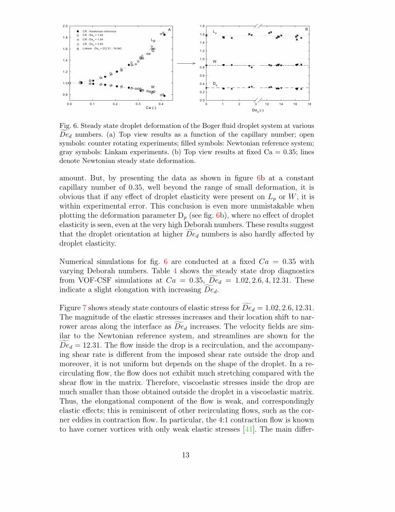
Fig. 6. Steady state droplet deformation of the Boger fluid droplet system at variousD̃ed numbers. (a) Top view results as a function of the capillary number; opensymbols: counter rotating experiments; filled symbols: Newtonian reference system;gray symbols: Linkam experiments. (b) Top view results at fixed Ca = 0.35; linesdenote Newtonian steady state deformation.

amount. But, by presenting the data as shown in figure 6b at a constantcapillary number of 0.35, well beyond the range of small deformation, it isobvious that if any effect of droplet elasticity were present on Lp or W , it iswithin experimental error. This conclusion is even more unmistakable whenplotting the deformation parameter Dp (see fig. 6b), where no effect of dropletelasticity is seen, even at the very high Deborah numbers. These results suggestthat the droplet orientation at higher D̃ed numbers is also hardly affected bydroplet elasticity.

Numerical simulations for fig. 6 are conducted at a fixed Ca = 0.35 withvarying Deborah numbers. Table 4 shows the steady state drop diagnosticsfrom VOF-CSF simulations at Ca = 0.35, D̃ed = 1.02, 2.6, 4, 12.31. Theseindicate a slight elongation with increasing D̃ed.

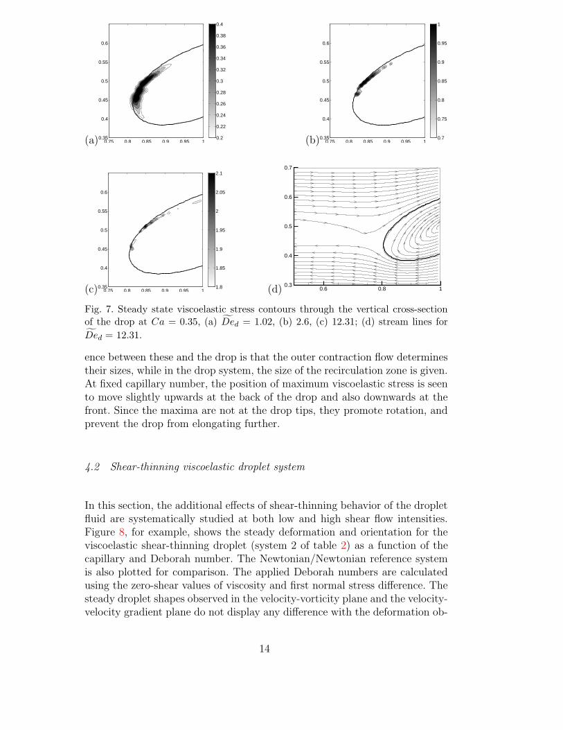
Figure 7 shows steady state contours of elastic stress for D̃ed = 1.02, 2.6, 12.31.The magnitude of the elastic stresses increases and their location shift to nar-rower areas along the interface as D̃ed increases. The velocity fields are sim-ilar to the Newtonian reference system, and streamlines are shown for theD̃ed = 12.31. The flow inside the drop is a recirculation, and the accompany-ing shear rate is different from the imposed shear rate outside the drop andmoreover, it is not uniform but depends on the shape of the droplet. In a re-circulating flow, the flow does not exhibit much stretching compared with theshear flow in the matrix. Therefore, viscoelastic stresses inside the drop aremuch smaller than those obtained outside the droplet in a viscoelastic matrix.Thus, the elongational component of the flow is weak, and correspondinglyelastic effects; this is reminiscent of other recirculating flows, such as the cor-ner eddies in contraction flow. In particular, the 4:1 contraction flow is knownto have corner vortices with only weak elastic stresses [41]. The main differ-

13

(a)

0.75 0.8 0.85 0.9 0.95 10.35

0.4

0.45

0.5

0.55

0.6

0.2

0.22

0.24

0.26

0.28

0.3

0.32

0.34

0.36

0.38

0.4

(b)

0.75 0.8 0.85 0.9 0.95 10.35

0.4

0.45

0.5

0.55

0.6

0.7

0.75

0.8

0.85

0.9

0.95

1

(c)

0.75 0.8 0.85 0.9 0.95 10.35

0.4

0.45

0.5

0.55

0.6

1.8

1.85

1.9

1.95

2

2.05

2.1

(d) 0.6 0.8 10.3

0.4

0.5

0.6

0.7

Fig. 7. Steady state viscoelastic stress contours through the vertical cross-sectionof the drop at Ca = 0.35, (a) D̃ed = 1.02, (b) 2.6, (c) 12.31; (d) stream lines for

D̃ed = 12.31.

ence between these and the drop is that the outer contraction flow determinestheir sizes, while in the drop system, the size of the recirculation zone is given.At fixed capillary number, the position of maximum viscoelastic stress is seento move slightly upwards at the back of the drop and also downwards at thefront. Since the maxima are not at the drop tips, they promote rotation, andprevent the drop from elongating further.

4.2 Shear-thinning viscoelastic droplet system

In this section, the additional effects of shear-thinning behavior of the dropletfluid are systematically studied at both low and high shear flow intensities.Figure 8, for example, shows the steady deformation and orientation for theviscoelastic shear-thinning droplet (system 2 of table 2) as a function of thecapillary and Deborah number. The Newtonian/Newtonian reference systemis also plotted for comparison. The applied Deborah numbers are calculatedusing the zero-shear values of viscosity and first normal stress difference. Thesteady droplet shapes observed in the velocity-vorticity plane and the velocity-velocity gradient plane do not display any difference with the deformation ob-

14

Fig. 8. Steady state droplet deformation and orientation. Open symbols:Shear-thinning viscoelastic branched fluid droplet - Newtonian matrix system (Sys-

tem 2 of table 2) at various D̃ed0 numbers; filled symbols: Newtonian referencesystem.

served for the Newtonian/Newtonian reference system. Also the orientation ofthe droplet is similar to that observed for the Newtonian reference system. Thedrop thus behaves like the Newtonian case, just as the Boger fluid droplet ofthe previous section, even at capillary numbers beyond the small deformationlimit.

Figure 9a shows the steady droplet deformation of the viscoelastic shear-thinning droplet, observed in the velocity-vorticity plane at very high Deborahnumbers, i.e. smaller droplets. The data are obtained with the Linkam shearcell, studying individual droplets. The steady droplet deformations, measuredwith the counter rotating setup are also displayed. It is shown that even atvery large Deborah numbers (D̃ed0 up to 12), or equivalent imposed shearrates up to 3 s−1, the effect of droplet elasticity and shear-thinning behavioris insignificant, although somewhat more scatter is observed in the Linkamexperiments. This becomes more obvious if the results are plotted versus the

15

Fig. 9. Steady state droplet deformation of the shear-thinning viscoelastic branchedfluid droplet system at various D̃ed0 numbers. (a) Top view results as a functionof the capillary number; open symbols: counter rotating experiments; filled sym-bols: Newtonian reference system; gray symbols: Linkam experiments. (b) Top viewresults at fixed Ca = 0.35; lines denote Newtonian steady state deformation.

Deborah number, as shown in figure 9b at a constant capillary number of0.35. The lines represent the corresponding Newtonian steady deformation. Itis obvious that if any effect of droplet elasticity and shear-thinning behaviorwould be present, it is small and within experimental error.

As in the previous section (e.g., fig. 5), numerical simulations with the Oldroyd-B model at βd0 = 0.6 produce similar droplet history as the Newtonian case.Introducing the shear-thinning by means of a Giesekus model, thereby resem-bling the rheology fitted with the Ellis model as exactly as possible, does nothave a pronounced effect on the resulting steady deformation and orientation.Therefore, the numerical results are omitted here since they mirror those ofthe previous section. This result is however not surprising, the shear rate in-side the droplet is much smaller than the imposed shear rate, and the elasticstresses generated by the recirculation inside the droplet are small, similar towhat is shown for the Boger fluid droplet system (see fig. 7).

4.3 Boger fluid matrix system

In figure 10, the steady droplet deformation and orientation for a Newtoniandrop - Boger fluid matrix (system 3 of table 2) are plotted as a function ofcapillary and Deborah number, together with the Newtonian reference sys-tem. This clearly shows two primary effects of introducing matrix elasticity,comparable to the results at other viscosity ratios [7, 8]: (i) to promote droporientation towards the flow direction even at low flow intensities, and (ii) tosuppress droplet deformation at higher capillary numbers. These and previ-ous data, do however not allow validation of the non-monotonous dependencyof the stationary droplet deformation on matrix viscoelasticity as obtainedwith the 2D simulations by Yue et al [22]. Therefore, the stationary droplet

16

Fig. 10. Steady state droplet deformation and orientation. Open symbols: Newtoniandroplet - Boger fluid matrix system (System 3 of table 2) at various D̃em numbers;filled symbols: Newtonian reference system.

deformation and orientation at higher Deborah numbers are addressed in fig-ure 11a .

Figure 11a shows the steady droplet deformation of the Boger fluid matrixsystem, observed in the velocity-vorticity plane, plotted as a function of theDeborah number (up to 16) at Ca = 0.35. It is shown that at D̃em ≈ 2, theeffect of matrix elasticity saturates. The dependency at lower Deborah number(< 2) is similar to that obtained for the BF2 matrix system with a viscosityratio of 0.75, studied in Verhulst et al. [8], and replotted here in figure 11b.Both experiments thus qualitatively yield the same results. At D̃em < 2, adecrease in droplet size, or equivalently, an increase in the applied D̃em, resultsin a decrease of the steady droplet deformation. A sigmoidal dependency onthe Deborah number is seen with an inflexion point around D̃em ≈ 1; thepoint where non-Newtonian effects are expected to become visible [4].

These experimentally observed trends are at least qualitatively predicted by

17

Fig. 11. Steady state droplet deformation of Boger fluid matrix system at variousD̃em numbers. (a) Steady droplet deformation observed in the velocity-vorticityplane at Ca = 0.35, lines denote Newtonian steady state deformation. (b) BF2 datataken from [8] at Ca = 0.35 and viscosity ratio 0.75.

the various phenomenological models presented in literature [8, 9, 10, 11],although they are predicting a monotonous decrease of the droplet deformationwith increasing D̃em. Hence, the quantitative prediction of these models athigh capillary numbers is less satisfying. Verhulst et al. [8] attribute this tothe simplicity of the rheological model used by [10]. Hence, in the numericalsimulations, the Oldroyd-B model is chosen to describe the rheology of theBoger fluid. Numerical simulations are conducted at Ca = 0.154, 0.35, or0.361, and compared with the data of figures 10 and 11a.

Simulations at low capillary number agree quite well with experimental data,as exemplified by fig. 12 at Ca = 0.154 and D̃em = 1.89, with λ = 1.5,βm = 0.68. Both deformation and angle of inclination are shown to be closelypredicted. Contours of viscoelastic stresses at t̂ = 10, 15, 30 are also shownin the figure. As time progresses, the area of largest viscoelastic stress movesfrom the drop tip slightly upwards. In figure 13, simulations with Ca = 0.154,and a D̃em increasing from 0 to 4, are shown because the experimental datashow saturation in D as the Deborah number increases. For higher Deborahnumbers, more mesh refinement is required and the initial transient takeslonger. Numerical results in fig. 13 also show little change in the stationarydeformation between D̃em = 0.5 and 2, and a slight decrease thereafter. Dueto spatial periodicity of the drop in the x-direction, contours may enter fromthe left boundary, as for the case D̃em = 6. To obtain fig. 13, higher numericalrefinements are used for D̃em ≥ 1.89.

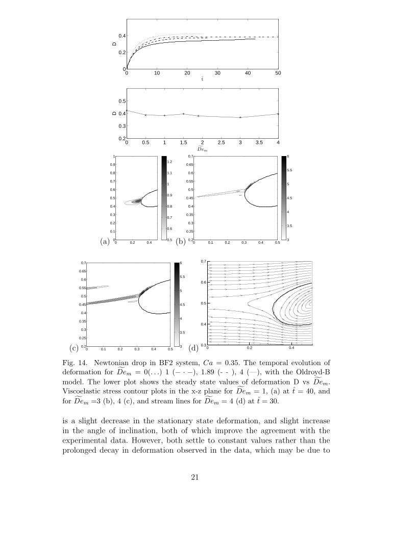
At higher capillary number, Ca = 0.35, simulations with the Oldroyd-B modelalso show saturation for the higher Deborah numbers, as shown in fig. 14. Theupper plot shows the evolution of deformation for D̃em = 0(. . .) 1 (−·−), 1.89(- - ), 4 (—), with the Oldroyd-B model. Again, the transients take longer tosettle with increasing Deborah number and D̃em = 4 is still slightly elongatingin the figure. In the lower figure, the deformation values vs D̃em show littlechange for the higher Deborah numbers, as in the 2D simulations of [22]. The

18

0 10 20 30 40 500

0.05

0.1

0.15

0.2

D

0 10 20 30 40 5025

30

35

40

45

θ

t̂

1

0 0.2 0.40

0.1

0.2

0.3

0.4

0.5

0.6

0.7

0.8

0.9

1

0.3

0.35

0.4

0.45

0.5

0.55

0.6

0.65

0.7

0.75

0.8

0 0.2 0.40

0.1

0.2

0.3

0.4

0.5

0.6

0.7

0.8

0.9

1

0.3

0.35

0.4

0.45

0.5

0.55

0.6

0.65

0.7

0.75

0.8

0 0.2 0.40

0.1

0.2

0.3

0.4

0.5

0.6

0.7

0.8

0.9

1

0.3

0.35

0.4

0.45

0.5

0.55

0.6

0.65

0.7

0.75

0.8

Fig. 12. Newtonian drop in an Oldroyd-B matrix with Ca = 0.154, D̃em = 1.89,λ = 1.5, βm = 0.68; o experimental data, — VOF-CSF simulation. Drop shapes andviscoelastic stress levels through the vertical cross-section at drop center are shownat t̂ = 10, 15, 30.

viscoelastic stress contours are shown at D̃em = 1, 3, 4 at fixed t̂ = 40. Thelocation of the maxima lie slightly above the drop tip at the back of the droprather than at the drop tips, directly at the interface. The streamlines areshown in the x − z cross-section for D̃em = 4, and the dividing streamlineappears to correspond with the high viscoelastic stresses that come off of thedrop in a narrow region.

Figure 15 shows temporal evolution for the particular case of Ca = 0.35,D̃em = 1.89, for experimental data (o) against the 3D Oldroyd B model (—)and the Giesekus model with κ̂m = 0.01. There is a slight decay in deformationin the Oldroyd B simulation for large time, but it essentially saturates to aconstant value of deformation and angle. The Giesekus model displays moredamping in the deformation and gives a better fit to the data. The data showsadditional damping as time progresses, which may reflect the presence of morethan one relaxation time. The effect of changing the retardation parameter in

19

0 5 10 15 20 25 30 35 400

0.05

0.1

0.15

0.2

D

t̂

1

0 0.5 1 1.5 2 2.5 3 3.5 40.1

0.15

0.2

D

D̃em

1

0 0.1 0.2 0.3 0.4 0.50.2

0.25

0.3

0.35

0.4

0.45

0.5

0.55

0.6

0.65

0.7

0.2

0.25

0.3

0.35

0.4

0.45

0.5

0 0.1 0.2 0.3 0.4 0.50.3

0.35

0.4

0.45

0.5

0.55

0.6

0.65

0.7

0.6

0.7

0.8

0.9

1

1.1

1.2

1.3

1.4

1.5

0 0.1 0.2 0.3 0.4 0.50.3

0.35

0.4

0.45

0.5

0.55

0.6

0.65

0.7

0.6

0.7

0.8

0.9

1

1.1

1.2

1.3

1.4

1.5

0 0.1 0.2 0.3 0.4 0.50.3

0.35

0.4

0.45

0.5

0.55

0.6

0.65

0.7

0.6

0.7

0.8

0.9

1

1.1

1.2

1.3

1.4

1.5

Fig. 13. Newtonian drop in BF2 system, modelled with Oldroyd-B. Ca = 0.154.The temporal evolution of deformation for D̃em = 0 (. . . ), 1 (− · −), 1.89 (−−),

4 (–), together with the steady state values of deformation D vs D̃em. Viscoelastic

stress contours for D̃em = 1, 1.89, 4, 6 at t̂ = 30.

the 3D simulations is that increasing from βm = 0.26 to βm = 0.8 decreasesthe maximum deformation. This provides a check that the value βm = 0.68deduced from table 3 is consistent.

The introduction of shear-thinning in the 3D simulation relieves the overallstress as shown in fig. 16. The left hand column shows the viscoelastic stressgrowing in intensity, while the addition of κ̂m = 0.01 is shown on the rightat the corresponding times. The effect of introducing the Giesekus parameter

20

0 10 20 30 40 500

0.2

0.4

D

t̂

1

0 0.5 1 1.5 2 2.5 3 3.5 40.2

0.3

0.4

0.5

D

D̃em

1

(a)

0 0.2 0.40

0.1

0.2

0.3

0.4

0.5

0.6

0.7

0.8

0.9

1

0.5

0.6

0.7

0.8

0.9

1

1.1

1.2

(b)

0 0.1 0.2 0.3 0.4 0.50.2

0.25

0.3

0.35

0.4

0.45

0.5

0.55

0.6

0.65

0.7

3

3.5

4

4.5

5

5.5

6

(c)

0 0.1 0.2 0.3 0.4 0.50.2

0.25

0.3

0.35

0.4

0.45

0.5

0.55

0.6

0.65

0.7

3

3.5

4

4.5

5

5.5

6

(d) 0 0.2 0.40.3

0.4

0.5

0.6

0.7

Fig. 14. Newtonian drop in BF2 system, Ca = 0.35. The temporal evolution ofdeformation for D̃em = 0(. . .) 1 (− · −), 1.89 (- - ), 4 (—), with the Oldroyd-B

model. The lower plot shows the steady state values of deformation D vs D̃em.Viscoelastic stress contour plots in the x-z plane for D̃em = 1, (a) at t̂ = 40, and

for D̃em =3 (b), 4 (c), and stream lines for D̃em = 4 (d) at t̂ = 30.

is a slight decrease in the stationary state deformation, and slight increasein the angle of inclination, both of which improve the agreement with theexperimental data. However, both settle to constant values rather than theprolonged decay in deformation observed in the data, which may be due to

21

0 10 20 30 40 500

0.1

0.2

0.3

0.4

D

0 10 20 30 40 5010

20

30

40

θ

t̂

1

Fig. 15. Newtonian drop in BF2 matrix with Ca = 0.36, D̃em = 1.89, λ = 1.5,βm = 0.68. Experimental data o; 3D Oldroyd-B model —; Giesekus model withκ̂m = 0.01 −·.

multiple relaxation times. The use of, for example, a 5-mode Giesekus modelthat accurately describes the linear viscoelasticity, the steady shear rheology,and steady and transient extensional rheology could be appropriate. Such afive mode Giesekus description of the BF2 is given in the Appendix. Notethat the simulations of [26] at the higher capillary numbers with the Oldroyd-B model overpredicts the viscoelastic stresses, and they use a Giesekus modelin order to compare with experimental data. In fact, this is due to an error intheir code which has been corrected for this paper.

5 Conclusion

The influence of matrix and droplet viscoelasticity on the steady deformationand orientation of a single droplet subjected to a homogeneous shear flow isinvestigated microscopically. The viscosity ratio is 1.5 and we focus on cap-illary numbers around 0.15 and 0.35, outside the range of small deformationasymptotics. Droplet viscoelasticity has hardly any effect on the steady dropletdeformation and orientation, even at moderate to high capillary and Debo-rah numbers. Matrix elasticity, on the other hand, significantly suppressesdroplet deformation and promotes droplet orientation, two effects that sat-urate at high Deborah numbers. This corresponds to decreasing the dropletradius under the same physical conditions. These experimental results are inquantitative agreement with 3D simulations performed with the Oldroyd-Bmodel; accurate results for the higher capillary number are obtained numeri-cally for the first time. The 3D simulations also show for the first time that thestationary value of deformation saturates at higher matrix Deborah numbers,

22

t̂ = 5

0 0.1 0.2 0.3 0.4 0.50.2

0.25

0.3

0.35

0.4

0.45

0.5

0.55

0.6

0.65

0.7

0.15

0.2

0.25

0 0.1 0.2 0.3 0.4 0.50.2

0.25

0.3

0.35

0.4

0.45

0.5

0.55

0.6

0.65

0.7

0.15

0.2

0.25

t̂ = 10

0 0.1 0.2 0.3 0.4 0.50.2

0.25

0.3

0.35

0.4

0.45

0.5

0.55

0.6

0.65

0.7

0.6

0.7

0.8

0.9

1

1.1

1.2

1.3

1.4

1.5

0 0.1 0.2 0.3 0.4 0.50.2

0.25

0.3

0.35

0.4

0.45

0.5

0.55

0.6

0.65

0.7

0.6

0.7

0.8

0.9

1

1.1

1.2

1.3

1.4

1.5

t̂ = 30

0 0.1 0.2 0.3 0.4 0.50.2

0.25

0.3

0.35

0.4

0.45

0.5

0.55

0.6

0.65

0.7

1.5

2

2.5

3

0 0.1 0.2 0.3 0.4 0.50.2

0.25

0.3

0.35

0.4

0.45

0.5

0.55

0.6

0.65

0.7

1

1.1

1.2

1.3

1.4

1.5

1.6

1.7

1.8

1.9

2

Fig. 16. Viscoelastic stress contours through the vertical cross-section of a drop forfig. 15. Newtonian drop in an Oldroyd-B fluid (left) with Ca = 0.361, D̃em = 1.89,λ = 1.5, βm = 0.68, and Giesekus model with κ̂m = 0.01 (right) at t̂ = 5, 10, 30.

which is also observed in the experimental data. The introduction of someshear-thinning in the matrix fluid by means of a Giesekus model yields thetrend that the deformation is lower and the angle is higher, both of whichare in the direction of the data. Additionally, the experimental data show agreater decay in stationary state deformation over a longer time scale than isdescribed by the rheological models used in the numerical simulations. Thisis reconciled by the presence of more than one relaxation time. Indeed, the5-mode Giesekus model is developed for the BF2 liquid which gives a moreaccurate prediction of the linear viscoelasticity, the steady shear rheology, andsteady and transient extensional rheology.

23

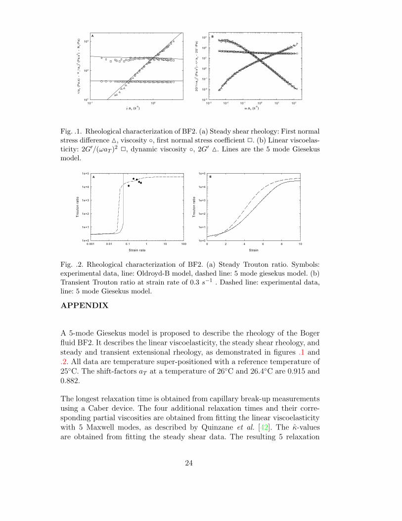
Fig. .1. Rheological characterization of BF2. (a) Steady shear rheology: First normalstress difference M, viscosity ◦, first normal stress coefficient 2. (b) Linear viscoelas-ticity: 2G′/(ωaT )2 2, dynamic viscosity ◦, 2G′ M. Lines are the 5 mode Giesekusmodel.

Fig. .2. Rheological characterization of BF2. (a) Steady Trouton ratio. Symbols:experimental data, line: Oldroyd-B model, dashed line: 5 mode giesekus model. (b)Transient Trouton ratio at strain rate of 0.3 s−1 . Dashed line: experimental data,line: 5 mode Giesekus model.

APPENDIX

A 5-mode Giesekus model is proposed to describe the rheology of the Bogerfluid BF2. It describes the linear viscoelasticity, the steady shear rheology, andsteady and transient extensional rheology, as demonstrated in figures .1 and.2. All data are temperature super-positioned with a reference temperature of25◦C. The shift-factors aT at a temperature of 26◦C and 26.4◦C are 0.915 and0.882.

The longest relaxation time is obtained from capillary break-up measurementsusing a Caber device. The four additional relaxation times and their corre-sponding partial viscosities are obtained from fitting the linear viscoelasticitywith 5 Maxwell modes, as described by Quinzane et al. [42]. The κ̂-valuesare obtained from fitting the steady shear data. The resulting 5 relaxation

24

times and their corresponding partial viscosities and κ̂-values; and the solventviscosity are given in table 5.

25

Acknowledgements

This research is supported by NSF-DMS-0456086, NCSA CTS060022, GOA03/06 and FWO-Vlaanderen for a fellowship for Ruth Cardinaels. The authorswould like to thank Prof. Shridhar of Monash University for measuring theextensional rheology of our samples, and Pascal Gillioen & Dr. Jorg Laugerof Anton Paar for their help with the counter rotating device.

References

[1] R.G. Larson. The structure and rheology of complex fluids. Oxford Uni-versity Press, 1999.

[2] L. A. Utracki. Polymer alloys and blends. Hanser Munich, 1989.[3] S. Guido and F. Greco. Dynamics of a liquid drop in a flowing immiscible

liquid. In D. M. Binding and K. Walters, editors, Rheology Reviews, pages99–142. British Society of Rheology, 2004.

[4] F. Greco. Drop deformation for non-Newtonian fluids in slow flows. J.

Non-Newtonian Fluid Mech., 107:111–131, 2002.[5] W. Yu, M. Bousmina, C. Zhou, and C. L. Tucker. Theory for drop de-

formation in viscoelastic systems. J. Rheol., 48(2):417–438, 2004.[6] S. Guido, M. Simeone, and F. Greco. Effects of matrix viscoelasticity

on drop deformation in dilute polymer blends under slow shear flow.Polymer, 44:467–471, 2003.

[7] S. Guido, M. Simeone, and F. Greco. Deformation of a Newtonian dropin a viscoelastic matrix under steady shear flow. Experimental validationof slow flow theory. J. Non-Newtonian Fluid Mech., 114:65–82, 2003.

[8] K. Verhulst, P. Moldenaers, and M. Minale. Drop shape dynamics of aNewtonian drop in a non-Newtonian matrix during transient and steadyshear flow. J. Rheol., 51:261–273, 2007.

[9] P. L. Maffettone and F. Greco. Ellipsoidal drop model for single dropdynamics with Non-Newtonian fluids. J. Rheol., 48:83–100, 2004.

[10] M. Minale. Deformation of a non-Newtonian ellipsoidal drop in anon-Newtonian matrix: extension of Maffettone-Minale model. J. Non-

Newtonian Fluid Mech., 123:151–160, 2004.[11] W. Yu, C. Zhou, and M. Bousmina. Theory of morphology evolution in

mixtures of viscoelastic immiscible components. J. Rheol., 49:215–236,2005.

[12] P. L. Maffettone, F. Greco, M. Simeone, and S. Guido. Analysis of start-up dynamics of a single drop through an ellipsoidal drop model for non-Newtonian fluids. J. Non-Newtonian Fluid Mech., 126:145–151, 2005.

[13] V. Sibillo, S. Guido, F. Greco, and P.L. Maffettone. Single drop dynamics

26

under shearing flow in systems with a viscoelastic phase. In Times of

Polymers, Macromolecular Symposiam 228, pages 31–39. Wiley, 2005.[14] V. Sibillo, M. Simeone, S. Guido, F. Greco, and P.L. Maffettone. Start-

up and retraction dynamics of a Newtonian drop in a viscoelastic matrixunder simple shear flow. J. Non-Newtonian Fluid Mech., 134:27–32, 2006.

[15] D. C. Tretheway and L. G. Leal. Deformation and relaxation of Newto-nian drops in planar extensional flow of a Boger fluid. J. Non-Newtonian

Fluid Mech., 99:81–108, 2001.[16] F. Mighri, A. Ajji, and P. J. Carreau. Influence of elastic properties on

drop deformation in elongational flow. J. Rheol., 41(5):1183–1201, 1997.[17] H. B. Chin and C. D. Han. Studies on droplet deformation and breakup.

i. droplet deformation in extensional flow. J. Rheol., 23(5):557–590, 1979.[18] W. J. Milliken and L. G. Leal. Deformation and breakup of viscoelastic

drops in planar extensional flows. J. Non-Newtonian Fluid Mech., 40:355–379, 1991.

[19] H. Vanoene. Modes of dispersion of viscoelastic fluids in flow. J. Colloid

Interface Sci., 40(3):448–467, 1972.[20] J. J. Elmendorp and R. J. Maalcke. A study on polymer blending mi-

crorheology: Part 1. Polym. Eng. Sci., 25:1041–1047, 1985.[21] F. Mighri, P. J. Carreau, and A. Ajji. Influence of elastic properties on

drop deformation and breakup in shear flow. J. Rheol., 42:1477–1490,1998.

[22] P. Yue, J. J. Feng, C. Liu, and J. Shen. Viscoelastic effects on dropdeformation in steady shear. J. Fluid Mech., 540:427 – 437, 2005.

[23] W. Lerdwijitjarud, R. G. Larson, A. Sirivat, and M. J. Solomon. Influ-ence of weak elasticity of dispersed phase on droplet behavior in shearedpolybutadiene/poly(dimethyl siloxane) blends. J. Rheol., 47(1):37–58,2003.

[24] W. Lerdwijitjarud, A. Sirivat, and R. G. Larson. Influence of dispersed-phase elasticity on steady-state deformation and breakup of droplets insimple shearing flow of immiscible polymer blends. J. Rheol., 48(4):843–862, 2004.

[25] N. Aggarwal and K. Sarkar. Deformation and breakup of a viscoelasticdrop in a Newtonian matrix under steady shear. J. Fluid Mech., 584:1–21,2007.

[26] D. Khismatullin, Y. Renardy, and M. Renardy. Development and imple-mentation of VOF-PROST for 3d viscoelastic liquid-liquid simulations.J. Non-Newtonian Fluid Mech., 140:120–131, 2006.

[27] S. B. Pillapakkam and P. Singh. A level-set method for computing solu-tions to viscoelastic two-phase flow. J. Comp. Phys., 174:552–578, 2001.

[28] T. Chinyoka, Y. Renardy, M. Renardy, and D. B. Khismatullin. Two-dimensional study of drop deformation under simple shear for Oldroyd-Bliquids. J. Non-Newtonian Fluid Mech., 130:45–56, 2005.

[29] H. K. Ganpule and B. Khomami. A theoretical investigation of interfacialinstabilities in the three layer superposed channel flow of viscoelastic

27

fluids. J. Non-Newtonian Fluid Mech., 79:315–360, 1998.[30] Y. Renardy and M. Renardy. Instability due to second normal stress

jump in two-layer shear flow of the Giesekus fluid. J. Non-Newtonian

Fluid Mech., 81:215–234, 1999.[31] J. Li, Y. Renardy, and M. Renardy. Numerical simulation of breakup of

a viscous drop in simple shear flow through a volume-of-fluid method.Phys. Fluids, 12(2):269–282, 2000.

[32] Y. Renardy and M. Renardy. PROST: a parabolic reconstruction of sur-face tension for the volume-of-fluid method. J. Comp. Phys., 183(2):400–421, 2002.

[33] Y. Renardy and J. Li. Parallelized simulations of two-fluid dispersions.SIAM News, 33(10):1, 2000.

[34] A. Vananroye, P. Van Puyvelde, and P. Moldenaers. Effect of confinementon droplet breakup in sheared emulsions. Langmuir, 22:3972–3974, 2006.

[35] A. Vananroye, P. Van Puyvelde, and P. Moldenaers. Effect of confine-ment on the steady-state behavior of single droplets during shear flow. J.

Rheol., 51(1):139–153, 2007.[36] V. Cristini, J. Blawzdziewicz, and M. Loewenberg. Drop breakup in

three-dimensional viscous flows. Phys. fluids, 10(8):1781–1783, 1998.[37] S. Guido, M. Simeone, and M. Villone. Diffusion effects on the interfacial

tension of immiscible polymer blends. Rheol. Acta, 38(4):287–296, 1999.[38] C. W. Macosko. Rheology principles, Measurements and Applications.

VCH Publishers, Inc., New York, 1994.[39] S. Guido and M. Villone. Three-dimensional shape of a drop under simple

shear flow. J. Rheol., 42:395–415, 1998.[40] A. Vananroye, P. Van Puyvelde, and P. Moldenaers. Structure develop-

ment in confined polymer blends: steady-state shear flow and relaxation.Langmuir, 22:2273–2280, 2006.

[41] P. Wapperom and M. F. Webster. Simulation for viscoelastic flow by afinite volume/element method. Computer Methods in Applied Mech. and

Engng., 180:281–304, 1999.[42] L.M. Quinzani, G.H. McKinley, R.A. Brown, and R.C. Armstrong. Mod-

eling the rheology of polyisobutylene solutions. J. Rheol., 34(5):705–748,1990.

28

Tables

∆x/R0 ∆tγ̇ D θ◦

1/8 0.0003 0.41 23.0

1/12 0.00014 0.40 23.5

1/16 0.00014 0.39 23.6

Table 1Tests for accuracy at D̃ed = 2.6, Ca = 0.35, t̂ = 30, λ = 1.5, Re = 0.05. The fluidpair is system 1 of table 2

Droplet Droplet phase Matrix phase Temp. Γ λ

-Matrix [◦C] [mN/m] [-]

1 VE–NE BF2 Saturated Rhodorsil 26.00±0.10 2.2±0.1 1.5

2 VE–NE BR16 Infineum mix 24.45±0.03 2.65±0.05 1.5

3 NE–VE Rhodorsil mix 1 BF2 26.40±0.04 2.0±0.1 1.5

4 NE–NE Rhodorsil mix 2 Parapol 1300 25.50±0.05 2.7±0.1 1.5

Table 2Blend characteristics at experimental conditions

Polymer Grade Temp. ηp ηs Ψ1 τ

[◦C] [Pa.s] [Pa.s] [Pa.s2] [s]

PIB Parapol 1300 25.50 83.5 . . . . . . . . .

Infineum mix 24.45 59.1 . . . . . . . . .

BF2 26.00 12.2 25.7 212 8.7

BF2 26.40 11.7 24.8 197 8.4

PDMS Rhodorsil mix 1 26.40 53.8 . . . . . . . . .

Rhodorsil mix 2 25.50 125 . . . . . . . . .

Saturated Rhodorsil 26.00 25.2 . . . . . . . . .

BR16 24.45 88.6a . . . 317b 1.8

Table 3Rheology of the blend components at experimental conditions. a The tabulated

viscosity is the zero shear viscosity obtained from a linear fit with Eq. 8, wherek = 0.4992 and n = 0.5430. b The tabulated Ψ1 is the zero shear first normalstress coefficient obtained from a logaritmic fit with Eq. 8, where k = 9.3550 andn = −0.0988.

29

D̃ed Lp W Dp L B D Angle

1.02 1.51 0.88 0.26 1.63 0.71 0.39 23

2.6 1.53 0.85 0.29 1.65 0.7 0.40 23

4 1.58 0.84 0.31 1.7 0.68 0.43 24

12.31 1.64 0.82 0.33 1.75 0.69 0.43 22

Table 4Numerical simulations for steady state of the elastic drop (system 1, table 2) at

Ca = 0.35. D̃ed = 1.02 (∆x = R0

8 ), 2.6 (∆x = R0

16 ), 4 (∆x = R0

8 ), 12.31 (∆x = R0

12 ).

Mode τ(s) ηp (Pa.s) κ̂

1 49 2.66 0.2

2 16.9 7.43 0.00001

3 2.03 5.82 0.00001

4 0.187 2.69 0.2

5 0.0131 1.39 0.2

Solvent - 27.2 -

Table 5Giesekus description with 5 relaxation modes of the BF2 fluid.

30

Figure captions

(1) Newtonian reference system with viscosity ratio 1.5 (system 4 of table 2).Experimental data (− · −) at Ca = 0.156 (lower), 0.363 (upper) arecompared with numerical simulations with the boundary integral code of[36] (−−) and VOF-CSF (—).

(2) Contour plots for viscoelastic stress for a Oldroyd-B drop in Newtonianmatrix, Ca = 0.35, D̃ed = 2.6, λ = 1.5, t̂ = 5 (row 1), 10 (row 2), 15(row 3); refinement left to right ∆x = R0/8, R0/12, R0/16.

(3) Rheological characterization of the viscoelastic fluids at a reference tem-perature of 25 ◦C. (a) PIB Boger fluid BF2. First normal stress dif-ference: M, viscosity: ♦, first normal stress coefficient: ◦; Lines are theOldroyd-B model. (b) Branched PDMS BR16. Open symbols are dy-namic data, 2G′/(ωaT )2: ◦, dynamic viscosity: ♦, 2G′: M; filled symbolsare steady shear data, first normal stress coefficient: •, viscosity: ¨, firstnormal stress difference: N; Lines are the Ellis model.

(4) Steady state droplet deformations and orientation. Open symbols: Bogerfluid droplet - Newtonian matrix system (System 1 of table 2) at variousD̃ed; filled symbols: Newtonian reference system.

(5) Side view deformation, 3D VOF-CSF simulation (—) and experimentaldata (− · −) at fixed D̃ed = 1.54, for Ca = (a) 0.14; (b) 0.32, andNewtonian CSF simulation (−−). The contours for viscoelastic stressesat stationary states are given.

(6) Steady state droplet deformation of the Boger fluid droplet system atvarious D̃ed numbers. (a) Top view results as a function of the capil-lary number; open symbols: counter rotating experiments; filled symbols:Newtonian reference system; gray symbols: Linkam experiments. (b) Topview results at fixed Ca = 0.35; lines denote Newtonian steady statedeformation.

(7) Steady state viscoelastic stress contours through the vertical cross-sectionof the drop at Ca = 0.35, D̃ed = 1.02 (a), 2.6 (b), 12.31(c), and streamlines for D̃ed = 12.31 (d).

(8) Steady state droplet deformation and orientation. Open symbols: Shear-thinning viscoelastic branched fluid droplet - Newtonian matrix system(System 2 of table 2) at various D̃ed0 numbers; filled symbols: Newtonianreference system.

(9) Steady state droplet deformation of the shear-thinning viscoelastic branchedfluid droplet system at various D̃ed0 numbers. (a) Top view results as afunction of the capillary number; open symbols: counter rotating experi-ments; filled symbols: Newtonian reference system; gray symbols: Linkamexperiments. (b) Top view results at fixed Ca = 0.35; lines denote New-tonian steady state deformation.

(10) Steady state droplet deformation and orientation. Open symbols: Newto-nian droplet - Boger fluid matrix system (System 3 of table 2) at variousD̃em numbers; filled symbols: Newtonian reference system.

31

(11) Steady state droplet deformation of Boger fluid matrix system at variousD̃em numbers. (a) Steady droplet deformation observed in the velocity-vorticity plane at Ca = 0.35, lines denote Newtonian steady state defor-mation. (b) BF2 data taken from [8] at a Ca = 0.35 and a viscosity ratioof 0.75.

(12) Newtonian drop in an Oldroyd-B matrix with Ca = 0.154, D̃em = 1.89,λ = 1.5, βm = 0.68; o experimental data, — VOF-CSF simulation. Dropshapes and viscoelastic stress levels through the vertical cross-section atdrop center are shown at t̂ = 10, 15, 30.

(13) Newtonian drop in BF2 system, modelled with Oldroyd-B. Ca = 0.154.The temporal evolution of deformation for D̃em = 0 (· · ·), 1 (− ·−), 1.89(−−), 4 (–), together with the steady state values of deformation D vsD̃em. Viscoelastic stress contours for D̃em = 1, 1.89, 4, 6 at t̂ = 30.

(14) Newtonian drop in BF2 system, Ca = 0.35. The temporal evolution ofdeformation for D̃em = 0(. . .) 1 (− · −), 1.89 (- - ), 4 (—), with theOldroyd-B model. The lower plot shows the steady state values of defor-mation D vs D̃em. Viscoelastic stress contour plots in the x-z plane forD̃em = 1, (a) at t̂ = 40, and for D̃em =3 (b), 4 (c), and stream lines forD̃em = 4 (d) at t̂ = 30.

(15) Newtonian drop in BF2 matrix with Ca = 0.36, D̃em = 1.89, λ = 1.5,βm = 0.68. Experimental data o; 3D Oldroyd-B model —; Giesekus modelwith κ̂m = 0.01 −·.

(16) Viscoelastic stress contours through the vertical cross-section of a dropfor fig. 15. Newtonian drop in an Oldroyd-B fluid (left) with Ca = 0.361,D̃em = 1.89, λ = 1.5, βm = 0.68, and Giesekus model with κ̂m = 0.01(right) at t̂ = 5, 10, 30.

(17) Viscoelastic stress contours through the vertical cross-section for 2D Oldroyd-B simulation in fig. 15. Newtonian drop in an Oldroyd-B fluid (left) withCa = 0.361, D̃em = 1.89, λ = 1.5, βm = 0.68, t̂ = 15, close to stationarystate.

(1) (Appendix) Rheological characterization of BF2. (a) Steady shear rhe-ology: First normal stress difference M, viscosity ◦, first normal stresscoefficient 2. (b) Linear viscoelasticity: 2G′/(ωaT )2

2, dynamic viscos-ity ◦, 2G′ M. Lines are the 5 mode Giesekus model.

(2) (Appendix) Rheological characterization of BF2. (a) Steady Trouton ra-tio. Symbols: experimental data, line: Oldroyd-B model, dashed line: 5mode giesekus model. (b) Transient Trouton ratio at strain rate of 0.3 s−1

. Dashed line: experimental data, line: 5 mode Giesekus model.

32