Engineering Fracture Mechanics 104 (2013) 29–40

Contents lists available at SciVerse ScienceDirect

Engineering Fracture Mechanics

journal homepage: www.elsevier .com/locate /engfracmech

Influence of the load history on the edge strength of glasswith arrised and ground edge finishing

0013-7944/$ - see front matter � 2013 Elsevier Ltd. All rights reserved.http://dx.doi.org/10.1016/j.engfracmech.2013.03.016

⇑ Corresponding author at: Laboratory for Research on Structural Models, Department of Structural Engineering, Ghent University, TechnoloZwijnaarde 904, B-9052 Ghent, Belgium. Tel.: +32 486154876.

E-mail address: marc.vandebroek@UGent.be (M. Vandebroek).

Marc Vandebroek a,b,⇑, Jan Belis a, Christian Louter c, Robby Caspeele d

a Laboratory for Research on Structural Models, Department of Structural Engineering, Ghent University, Technologiepark-Zwijnaarde 904, B-9052 Ghent, Belgiumb Faculty of Design Sciences, Artesis University College, Antwerp University Association, Mutsaardstraat 31, B-2000 Antwerp, Belgiumc Steel Structures Laboratory (ICOM), École Polytechnique Fédérale de Lausanne (EPFL), School of Architecture, Civil and Environmental Engineering (ENAC), GCB3 505, Station 18, CH-1015 Lausanne, Switzerlandd Magnel Laboratory for Concrete Research, Department of Structural Engineering, Ghent University, Technologiepark-Zwijnaarde 904, B-9052 Ghent, Belgium

a r t i c l e i n f o

Article history:Received 30 April 2012Received in revised form 27 December 2012Accepted 19 March 2013Available online 30 March 2013

Keywords:Structural glassEdge strengthLoad historyFracture mechanicsStress corrosion

a b s t r a c t

The edge strength of glass is affected by the load history. To quantify this effect, 12 series ofglass specimens were subjected to either linearly increased (reference value), constant orcyclic loading. For constant loading the experimental values could be accurately predictedby linear elastic fracture mechanics (LEFM). However, for cyclic loading the LEFM predic-tion was 4–8% more conservative than the test results. Furthermore, a comparison of theexperimental results with the prediction method provided in the standards shows thatfor cyclic loading the number of cycles should be taken into account in the rules of thestandards.

� 2013 Elsevier Ltd. All rights reserved.

1. Introduction

Designers tend to use glass more and more as a structural element. Consequently, the edges may be subjected to signif-icant tensile stresses, as in structural glass beams or façade mullions. In secondary construction elements such as windows,the edges may be subjected to considerable tensile stresses due to e.g. thermal actions. However, the edge strength, which ishighly dependent on the edge finishing, is – in contrast to the surface strength – insufficiently documented in literature andacknowledged in the existing standards [1,2]. In particular, experimental results of cyclic testing are scarcely documented inliterature.

Prior to thermal fracture, the edges of a pane are usually subjected to an enormous number of cycles during the lifetime ofthe pane. These cycles provoke static fatigue due to stress corrosion. In order to decide whether the largest stress during thelife of a pane or the much lower equivalent cyclic stress is more relevant, a precise estimation of the strength under cyclicloading is of major importance.

In this study, 12 series of specimens, with either arrised or ground edge finishing and a thickness of either 4 or 8 mm,were tested in a four-point bending setup. First, four series were subjected to a linearly increased loading (constant stressrate, strength f). Then four series of specimens, identical to the previous series, were tested under constant loading (constantstress, strength fct). Finally, four series were tested under cyclic loading (cyclic constant stress, strength fcycl).

giepark-

Nomenclature

a flaw depthaci initial critical flaw depthac(t) critical flaw depth at time tb width of the specimend distance between the load and the supportf tensile strength corresponding to a constant stress ratefct tensile strength corresponding to a constant loadingfcycl tensile strength corresponding to a cyclic loadingfinert inert strengthh height of the specimenkmod factor for the load durationKI stress intensity factor in mode IKIc fracture toughness of modern soda-lime silica glassKth crack growth thresholdl inner span of the specimen (load span)L outer span of the specimenn crack velocity parameterP total loadPf experimental failure loadt timetf time period during which the flaw can resist the stress historytload load duration of the actionttest load duration of the testv crack velocityv0 crack velocity, when KI = KIc�x; s sample mean and sample standard deviationY geometry factorh,b parameters of the 2-parameter Weibull distribution

h_

,b_

estimated parameters of the 2-parameter Weibull distributionl,r parameters of the 2-parameter Lognormal distribution

l_;r_

estimated parameters of the 2-parameter Lognormal distributionrn maximum tensile stress, constant within the load spanrn(t) stress normal to the plane of the flaw at time t

30 M. Vandebroek et al. / Engineering Fracture Mechanics 104 (2013) 29–40

The first objective of this investigation is to assess if a methodology based on fracture mechanics and fracture statisticsthat explicitly incorporates slow growth of cracks can conservatively predict failure of glass under constant or cyclic load.

The second objective is to explore whether the test results correspond to the normative guidelines mentioned in thestandards.

For both objectives, the experimental data will be fitted to the Weibull and the lognormal distribution, to see whether theconclusions are depending upon the chosen distribution.

2. Test specimens and method

The nominal sizes of the soda lime silica glass specimens were 110 mm � 12.5 mm � 4 mm and 170 mm � 18.75 mm � 8 mm,see Figs. 1 and 2. The outer and inner span (or load span l) lengths were 100 mm and 40 mm, respectively, for the 4 mm spec-

Fig. 1. Schematic overview of the in-plane four-point bending test.

Fig. 2. (a) In-plane four-point bending test setup. (b) Detail of the in-plane four-point bending test setup.

Fig. 2. (continued)

M. Vandebroek et al. / Engineering Fracture Mechanics 104 (2013) 29–40 31

imens and 150 mm and 60 mm, respectively, for the 8 mm specimens. The edges had an arrised or ground edge finishing aslisted in Table 1. Before processing the edge, the cutting was performed by a qualified glass processer using a standard auto-mated cutting process. The latter was subjected to a strict protocol, according to which e.g. the scoring of the specimens oc-curred at the air side, i.e. the surface which is exposed to the air (atmosphere) during the float process. Grinding was donewith a diamond-grit wheel (D151, D91) and arrising was done with a belt sander (Corundum P80).

The specimens under study were subjected to in-plane four-point bending tests in an Instron 3369 testing machine at atest temperature of 20 �C ± 2 �C and a relative humidity of 65% ± 4%, with the air (atmospheric) side of the glass always in thesame position (Fig. 2). The specimens of 4 mm were loaded either at a stress rate of 2 MPa/s, a constant stress or a cyclicconstant stress (Fig. 3). For the cyclic constant stress, the holding phase amounted to 3 s and the time between the cyclesamounted to 5 s. The transition between the constant stress and no stress was performed at a stress rate of 50 MPa/s.The specimens of 8 mm were loaded at a stress rate of 0.08 MPa/s, a constant stress and a cyclic constant stress (Fig. 4).

0

10

20

30

40

50

60

70

0 100 200 300 400 500 600 700

stress rate: 0.08 MPa/sconstant stresscyclic constant stress

σ [MPa]

time [s]

failure

loading time: 3 s

load of 20N during 20 s

loading and unloading at 50 MPa/s

Fig. 4. Loading at constant stress rate, constant stress and cyclic constant stress, specimens of 8 mm (series G to L).

0

10

20

30

40

50

60

70

0 10 20 30 40

stress rate: 2 MPa/s constant stresscyclic constant stress

σ [MPa]

time [s]

failure

3 s loading and unloading at 50MPa/s

load of 20 N during 5 s

Fig. 3. Loading at constant stress rate, constant stress and cyclic constant stress, specimens of 4 mm (series A to F).

Table 1Overview of the test series.

Specimen thickness Edge finishing Stress rate (MPa/s) Number of specimens Series

4 mm Arrised Stress rate: 2 MPa/s 60 AConstant stress 30 BCyclic constant stress 30 C

Ground Stress rate: 2 MPa/s 60 DConstant stress 30 ECyclic constant stress 30 F

8 mm Arrised Stress rate: 0.08 MPa/s 60 GConstant stress 30 HCyclic constant stress 30 I

Ground Stress rate: 0.08 MPa/s 60 JConstant stress 30 KCyclic constant stress 30 L

32 M. Vandebroek et al. / Engineering Fracture Mechanics 104 (2013) 29–40

For the cyclic constant stress, the holding phase amounted to 3 s and the time between the cycles amounted to 20 s. Thetransition between the constant stress and no stress was performed at a stress rate of 50 MPa/s.

M. Vandebroek et al. / Engineering Fracture Mechanics 104 (2013) 29–40 33

An overview of these test series is given in Table 1. At least 90 days elapsed between processing the edge and testingthe specimens. During the 14 days before testing, the specimens were kept at a temperature of 20 �C ± 2 �C and a relativehumidity of 65% ± 4%, the same as the test conditions.

For a specific thickness and edge finishing, all the specimens (60 + 30 + 30) of the three series (constant stress rate, con-stant stress and cyclic stress: see Table 1) are prepared out of identical panes, of which the edge was processed on the sameday with the same machine and the same processing parameters. Consequently, for the comparison of the three loading his-tories for a certain thickness and edge finishing, one can assume the same flaw population caused by processing the edge.

During testing at a constant stress rate (Table 1: series A, D, G, J), the load P in function of the time was recorded, as well asthe time to failure tf. The specimens which failed outside the load span were excluded from the study.

During testing, the stress rn was given in function of the load P by:

rn ¼ðP=2Þ � dðb � h2Þ=6

¼ 3 � P � db � h2 ð1Þ

rn (MPa) is the maximum tensile stress, constant within the load span (Fig. 1), P (N) the total load (Fig. 1), d (mm) the dis-tance between the load and the support (Fig. 1), b (mm) the width of the specimen (Fig. 1) and h (mm) is the height of thespecimen (Fig. 1).

After testing, the failure stress values or tensile strength values f were calculated based on the failure loads Pf for series A,D, G, J (Table 1) with following equation:

f ¼ ðPf =2Þ � dðb � h2Þ=6

¼ 3 � Pf � db � h2 ð2Þ

f (MPa) is the tensile strength corresponding to a linearly increased loading (experimental result: specimen loaded at a con-stant stress rate) and Pf (N) is the experimental failure load

3. Fracture mechanics and stress corrosion

The theory of linear elastic fracture mechanics (LEFM) describes the relation between the tensile strength and the flawparameters, i.e. the flaw geometry and the flaw dimension.

Since Griffith [3] demonstrated that flaws determine the strength of glass, and because glass shows a perfectly elasticbehavior until failure, the linear elastic fracture mechanics (LEFM) theory is generally accepted in describing glass failurestrength.

According to the latter theory, at inert conditions, i.e. when no subcritical crack growth occurs, the general relationshipbetween the stress intensity factor KI (mode I), the constant tensile stress normal to the flaws plane rn, the geometry factor Yand the flaw depth a is given by Eq. (3) [4–7]:

KI ¼ Y � rn � ðp � aÞ1=2 ð3Þ

KI (MPa m1/2) is the stress intensity factor in mode I, Y (�) the geometry factor, rn (MPa) the tensile stress normal to theplane of the flaw (Fig. 5) and a (m) the flaw depth (Fig. 5)

Furthermore, according to LEFM, the critical stress intensity factor or fracture toughness is the stress intensity factorwhich leads to instantaneous failure (i.e. corresponding to the inert or short-term strength) [1,3,4]:

Thus KIc ¼ Y � finert � ðp � aciÞ1=2 ð4Þ

KIc = 0.75 MPa m1/2 is the fracture toughness of modern soda-lime silica glass [1,8], finert (MPa) the inert strength, aci (m) isthe initial critical flaw depth.

Fig. 5. Schematic view of the flaw, rn denotes the tensile stress normal to the flaws plane.

log v

v = v0(KI / KIc)n

Kth

II

log KI

III

KIc

v0

I

Fig. 6. Relationship between crack velocity and stress intensity [1].

34 M. Vandebroek et al. / Engineering Fracture Mechanics 104 (2013) 29–40

Considering stress corrosion and subcritical crack growth, the relation between the crack velocity v and the stress inten-sity factor KI is given by (Fig. 6: region I) [1,9,10]:

v ¼ v0 � ðKI=KIcÞn ð5Þ

v (m/s) is the crack velocity, v0 (m/s) the crack velocity, when KI = KIc and n (�) the crack velocity parameter: constant valueof 16 [11]

Since structural elements are generally expected to be in service for several years, only region I in Fig. 6 is of interest, i.e.the region with extremely slow subcritical crack growth. The contribution of regions II and III to an element’s lifetime is neg-ligible [12].

To find the relation between two different stress histories which result in the same crack growth, the differential equationof crack growth is integrated [1,6].

Eq. (5) can be written as follows:

v ¼ da=dt ¼ v0 � ðKI=KIcÞn ð6Þ

t (s) is the time.Using Eq. (3), integration of Eq. (6) yields [1,6]:

Z acðtÞ

aci

a�n=2da ¼Z t

0v0 � K�n

Ic ðY � p1=2Þn � rnnðtÞ � dt ð7Þ

aci (m) is the initial critical flaw depth, ac(t) (m) the critical flaw depth at time t and rn(t) (MPa) the stress normal to the planeof the flaw at time t.

Thus, with n being constant, Eq. (7) yields:

Z t

0rn

nðtÞ � dt ¼ 2

ðn� 2Þ � v0 � K�nIc ðY � p1=2Þn � aðn�2Þ=2

ci

ð1� ðaci=acðtÞÞðn�2Þ=2Þ ð8Þ

At failure time tf (or lifetime of the flaw under consideration), ac(t) equals ac(tf):

Z tf

0rn

nðtÞ � dt ¼ 2

ðn� 2Þ � v0 � K�nIc ðY � p1=2Þn � aðn�2Þ=2

ci

ð1� ðaci=acðtf ÞÞðn�2Þ=2Þ ð9Þ

tf (s) is the time period during which the flaw can resist the stress history.As n is large and assuming ac(tf)� aci, Eq. (9) yields [1,6]:

Z tf

0rn

nðtÞ � dt ¼ 2

ðn� 2Þ � v0 � K�nIc ðY � p1=2Þn � aðn�2Þ=2

ci

ð10Þ

Eq. (10) means that two stress histories rn1(t), t e [0,tf1] and rn2(t), t e [0, tf2] cause the same crack growth if:

Z tf 1

0rn

n1ðtÞ � dt ¼Z tf 2

0rn

n2ðtÞ � dt ð11Þ

The value of these integrals increases from 0 at the beginning of the loading to the value of Eq. (10) at failure [12]. The inte-gration will be performed for values of KI > Kth, Kth being the crack growth threshold [1,12,13].

M. Vandebroek et al. / Engineering Fracture Mechanics 104 (2013) 29–40 35

Comparing the strength values of two specimens tested at a different constant stress i.e. assuming a constant value ofrn1(t) = fct,1 and rn2(t) = fct,2, Eq. (11) yields:

fct;1=fct;2 ¼ ðtf ;ct;2=tf ;ct;1Þ1=n ð12Þ

4. Theoretical and experimental strength values

To compare theoretical and experimental strength values for the three different load histories, two different approachesare considered.

– In the first approach testing could be conducted at a constant stress rate at inert conditions (high stress rate and no influ-ence of humidity). Using Eq. (4), the distribution of the initial critical flaw depth aci can be determined if the geometryfactor Y is well known. However, in literature, the value of Y is not given for an edge flaw population. This could beachieved by measuring the initial critical flaw depth aci by means of microscopy. Unfortunately, this measurement is verydifficult to carry out. Next, using Eqs. (6), (10), failure times and their distribution for the specific loading history (constantstress rate) can be calculated, taking into account slow crack growth. However, the values of the stress corrosion param-eters n and v0 must be known in order to calculate the failure times. The first one is well known (n = 16) but the secondone v0 is not well known in literature for laboratory conditions. Again, this parameter v0 can be assessed by testing atambient conditions (at a constant stress rate i.e. linearly increased loading) by applying Eq. (10). The calculated failuretime distributions can then be compared with failure time distributions measured under constant load or cyclic loadexperiments.

– In the second approach testing could be conducted at ambient conditions (at a constant stress rate i.e. linearly increasedloading). Next, the measured failure time distributions of this linearly increased loading at ambient conditions are com-pared to those of the constant load or cyclic load experiments. All three load histories are executed under the same ambi-ent conditions (temperature of 20 �C ± 2 �C and relative humidity of 65% ± 4%), without assessment of the stress corrosionparameters.

Summarizing, for this article the second approach is followed, because:

(a) For the first approach, the geometry factor Y is not well known, and consequently the initial critical flaw depth aci ofeach specimen has to be measured by means of microscopy, which is very difficult.

(b) Testing with a linearly increased loading at ambient conditions is needed for both approaches. However, for the firstapproach this is needed additionally to the inert testing to determine the stress corrosion parameter v0. Consequently,the double amount of tests would be required to obtain the same goal.

(c) In both approaches, the assumption of the same flaw distribution for the three load histories has to be made, even ifone of them is measured (see point a above related) and the other two are implicitly reflected in the strength valuesand time to failure values (first approach). Also in the second approach, the same flaw distribution is reflected in thestrength values and the failure time values for the three load histories, as they are cut out of identical glass panes (seeSection 2). More precisely, the assumption which is made in the second approach is that the mean value of the dis-tribution of aci is identical for the three load histories (which are compared to each other). This assumption is reason-able, as the specimens are prepared from identical panes (see Section 2). Individual specimens are not comparedbetween two load histories, as the initial critical flaw depth aci can vary considerably between individual specimensin one series or in the other.

Applying the second approach, first, the series A, D, G and J were tested at a constant stress rate (ambient conditions at astress rate of 2 MPa/s or 0.08 MPa/s). These tests resulted in the experimental strength f. Then the series B, E, H and K weretested at a constant stress (load controlled testing). Theoretically, the magnitude of this constant stress was determined bymeans of Eq. (11). Therefore, experiments were first executed under the latter constant stress, aiming at the same time tofailure as the test with a constant stress rate, see Figs. 3 and 4. If the mean failure time of a certain number of specimenswas higher than the mean value of the corresponding series, tested at a constant stress rate, the level of the constant stresswas increased, and vice versa. In this way, the experimental strength fct was determined.

As the height of the individual specimens varied, the corresponding constant stress varied similarly when a constant loadwas applied for one series. However, as the variation of the height was similar for each load history and only the mean valueof the strength values and failure time values of all specimens of one serie was compared between different load histories,the followed procedure does not influence the accuracy.

Finally, the same procedure was followed for series C, F, I and L, which determined the experimental strength fcycl.The experimental results of f, fct, fcycl and the corresponding failure times tf, tf,ct, tf,cycl for series A to L were fitted to the 2-

parameter Weibull distribution (Eq. (13): probability density function with parameters h and b) and the 2-parameter lognor-mal distribution (Eq. (14): probability density function with parameters l and r), using the Maximum Likelihood Estimation(MLE) method:

Table 4Experim

Serie

CFIL

Table 2Experim

Serie

ADGJ

Table 3Experim

Serie

BEHK

36 M. Vandebroek et al. / Engineering Fracture Mechanics 104 (2013) 29–40

f ðxÞ ¼ bh� x

h

� �b�1exp � x

h

� �b� �

for x > 0 ð13Þ

f ðxÞ ¼ 1x � r �

ffiffiffiffiffiffiffi2pp � exp �1

2� ln x� l

r

� �2 !

for x > 0 ð14Þ

The Kolmogorov–Smirnov test was carried out to compare the goodness-of-fit to these two different distributions. In order tocompare the two distributions, the p-values were calculated. The p-value denotes the threshold value of the significance le-vel in the sense that the null hypothesis (H0: the data follow the specified distribution) will be accepted for all values of thesignificance level less than the p-value. In other words, the p-value is the smallest level of significance that would lead torejection of the null hypothesis H0 with the given data. For structural applications, a significance level of 5% is suggested,which is equivalent to a minimum p-value of 5%.

Considering these two distributions, the estimation of the mean value for the strength value f, or fct or fcycl was calculatedfor all test series. Subsequently, the estimation of the mean values for the time to failure tf, or tf,ct, or tf,cycl was calculated forall test series.

Theoretically, the magnitude of the constant strength value fct was calculated from Eq. (11) (rn1(t) being the stress history,testing under constant stress rate, failing after a period of time tf1; rn2(t) being the constant stress history by which the spec-imens fail after the same period of time tf,ct,2 = tf1). Thus, the theoretical ratio fct/f was calculated. This ratio was compared tothe experimental ratio. In the same way, the theoretical ratio fcycl/f, by using Eq. (11), was compared to the correspondingexperimental ratio. The results of this comparison are provided and discussed in Section 6.

5. Results

For all specimens, the origin of the failure was located.It was observed that for the arrised edges 74% of the failures occurred at the edges, 26% at the inclined surface between

two edges. For the three different load histories this ratio was similar (failures at the edge: constant stress rate: 69%, constantstress: 78%, cyclic constant stress: 75%).

It was observed that for the ground edges 79% of the failures occurred at the edges, 21% at the inclined surface betweentwo edges. For the three different load histories this ratio was similar (failures at the edge: constant stress rate: 81%, constantstress: 79%, cyclic constant stress: 75%).

For every series, the number of specimens, the sample mean �x of the strength and the time to failure and the correspond-ing sample standard deviation s are listed in Tables 2–4.

ental results of series C, F, I and L.

s Number of specimens [�] fcycl �x (MPa) s (MPa) tf,cycl �x (s) s (s)

30 45.5 1.3 28.3 22.130 61.9 1.5 32.9 35.330 45.1 0.7 571 27430 49.8 1.0 645 307

ental results of series A, D, G and J.

s Number of specimens (�) f �x (MPa) s (MPa) tf �x (s) s (s)

60 47.7 5.2 23.4 2.960 64.9 7.3 32.0 4.160 45.1 3.6 559 4960 49.9 3.2 616 38

ental results of series B, E, H and K.

s Number of specimens (�) fct �x (MPa) s (MPa) tf,ct �x (s) s (s)

30 40.4 1.0 25.7 26.730 54.5 0.9 37.8 48.030 37.8 0.8 581 40830 41.8 0.9 632 300

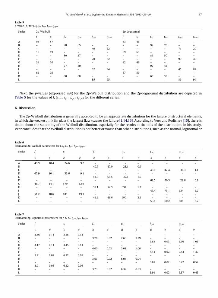
Table 5p-Value (%) for f, tf, fct, tf,ct, fcycl, tf,cycl.

Series 2p-Weibull 2p-Lognormal

f tf fct tf,ct fcycl tf,cycl f tf fct tf,ct fcycl tf,cycl

A 95 87 – – – – 53 46 – – – –B – – 98 65 – – – – 97 70 – –C – – – – 49 22 – – – – 71 20D 18 19 – – – – 69 65 – – – –E – – 80 27 – – – – 86 50 – –F – – – – 70 62 – – – – 90 40G 34 50 – – – – 42 49 – – – –H – – 77 80 – – – – 97 42 – –I – – – – 62 94 – – – – 45 82J 66 95 – – – – 87 59 – – – –K – – 90 68 – – – – 68 39 – –L – – – – 85 95 – – – – 86 94

M. Vandebroek et al. / Engineering Fracture Mechanics 104 (2013) 29–40 37

Next, the p-values (expressed in%) for the 2p-Weibull distribution and the 2p-lognormal distribution are depicted inTable 5 for the values of f, tf, fct, tf,ct, fcycl, tf,cycl for the different series.

6. Discussion

The 2p-Weibull distribution is generally accepted to be an appropriate distribution for the failure of structural elements,in which the weakest link (in glass the largest flaw) causes the failure [1,14,16]. According to Veer and Rodichev [15], there isdoubt about the suitability of the Weibull distribution, especially for the results at the tails of the distribution. In his study,Veer concludes that the Weibull distribution is not better or worse than other distributions, such as the normal, lognormal or

Table 6Estimated 2p-Weibull parameters for f, tf, fct, tf,ct, fcycl, tf,cycl.

Series f tf fct tf,ct fcycl tf,cycl

h_

b_

h_

b_

h_

b_

h_

b_

h_

b_

h_

b_

A 49.9 10.4 24.6 9.2 – – – – – – – –B – – – – 40.7 47.0 23.1 0.9 – – – –C – – – – – – – – 46.0 42.4 30.3 1.1D 67.9 10.1 33.6 9.1 – – – – – – – –E – – – – 54.9 69.5 32.1 1.0 – – – –F – – – – – – – – 62.5 50.5 29.6 0.9G 46.7 14.1 579 12.9 – – – – – – – –H – – – – 38.1 54.3 634 1.2 – – – –I – – – – – – – – 45.4 75.1 624 2.2J 51.2 18.6 631 19.1 – – – – – – – –K – – – – 42.3 49.6 690 2.2 – – – –L – – – – – – – – 50.1 60.2 688 2.7

Table 7Estimated 2p-lognormal parameters for f, tf, fct, tf,ct, fcycl, tf,cycl.

Series f tf fct tf,ct fcycl tf,cycl

l_

r_

l_

r_

l_

r_

l_

r_

l_

r_

l_

r_

A 3.86 0.11 3.15 0.13 – – – – – – – –B – – – – 3.70 0.02 2.60 1.29 – – – –C – – – – – – – – 3.82 0.03 2.96 1.03D 4.17 0.11 3.45 0.13 – – – – – – – –E – – – – 4.00 0.02 3.01 1.06 – – – –F – – – – – – – – 4.13 0.02 2.83 1.32G 3.81 0.08 6.32 0.09 – – – – – – – –H – – – – 3.63 0.02 6.04 0.94 – – – –I – – – – – – – – 3.81 0.02 6.22 0.52J 3.91 0.06 6.42 0.06 – – – – – – – –K – – – – 3.73 0.02 6.32 0.53 – – – –L – – – – – – – – 3.91 0.02 6.37 0.45

Table 8Corresponding mean values for f, tf, fct, tf,ct, fcycl, tf,cycl.

Series 2p-Weibull 2p-Lognormal

f (MPa) tf (s) fct (MPa) tf (s) fcycl (MPa) tf (s) f (MPa) tf (s) fct (MPa) tf (s) fcycl (MPa) tf (s)

A 47.6 23.3 – – – – 47.8 23.4 – – – –B – – 40.3 24.7 – – – – 40.4 30.7 – –C – – – – 45.4 29.7 – – – – 45.5 32.7D 64.6 31.9 – – – – 64.9 32.0 – – – –E – – 54.5 31.9 – – – – 54.5 35.5 – –F – – – – 61.8 32.1 – – – – 61.9 40.3G 45.0 556 – – – – 45.2 559 – – – –H – – 37.7 599 – – – – 37.8 654 – –I – – – – 45.1 553 – – – – 45.1 578J 49.8 614 – – – – 49.9 616 – – – –K – – 41.8 611 – – – – 41.8 641 – –L – – – – 49.7 612 – – – – 49.7 645

Table 9Theoretical and experimental ratio of fct/f and fcycl/f.

Series Theoretical 2p-Weibull 2p-Lognormal

Experimental dev. (%) Theoretical Experimental dev. (%)

fct/f (%) fcycl/f (%) fct/f (%) fcycl/f (%) fct/f (%) fcycl/f (%) fct/f (%) fcycl/f (%)

A–B 0.837 – 0.847 – 1.2 0.837 – 0.845 – 1A–C – 0.887 – 0.954 7.6 – 0.887 – 0.952 7.3D–E 0.837 – 0.843 – 0.7 0.837 – 0.84 – 0.4D–F – 0.906 – 0.956 5.5 – 0.906 – 0.954 5.3G–H 0.838 – 0.839 – 0.1 0.838 – 0.837 – –0.1G–I – 0.954 – 1.002 5 – 0.955 – 1 4.7J–K 0.838 – 0.839 – 0.1 0.838 – 0.838 – 0J–L – 0.956 – 0.998 4.4 – 0.956 – 0.997 4.3

38 M. Vandebroek et al. / Engineering Fracture Mechanics 104 (2013) 29–40

extreme value distribution. However, in other studies on structural glass also the 2p-lognormal distribution is used [13]. Asthe strength of glass is caused by the geometrical value of the flaw-depth, the latter distribution seems to be a suitableassumption as well.

In the current study, both distributions i.e. the Weibull distribution and the lognormal distribution are considered. Asshown in Table 5, most series resulted in the same magnitude of p-values for the 2p-Weibull distribution fitting and the2p-lognormal distribution fitting. As the p-values for these two distributions are all significantly larger than 5% (minimumsignificance level for structural applications), the 2p-Weibull distribution and the 2p-lognormal distribution are both accept-able probabilistic models for this study. Therefore, the following analysis was performed with both distribution types in or-der to illustrate the small differences in final results. The estimated 2p-Weibull parameters (h

_

and b_

) and 2p-lognormalparameters (l

_and r

_) for f, tf, fct, tf,ct, fcycl, tf,cycl are listed in Tables 6 and 7, respectively. Next, the corresponding mean values

for f, tf, fct, tf,ct, fcycl, tf,cycl are depicted in Table 8 (based on MLE).Applying Eq. (11), the theoretical ratio fct/f was calculated for the different series (see Table 9). This ratio was compared to

the experimental ratio, provided in Table 8. In the same way, the theoretical ratio fcycl/f was compared to the experimentalvalue. The deviation between the experimental ratio and the theoretical ratio was calculated:

dev: ¼ 100 � ðexperimental ratio� theoretical ratioÞ=theoretical ratio

It can be concluded from Table 9 that Eq. (11) yields a ratio of fct/f which is only 0.1% less to 1.2% more conservative thanthe experimental values (bold values of the dev.). Both the theoretical and experimental values of fct/f are all very close to thevalue found by Mencik [17], i.e. (1/(n + 1))1/n = 0.838. However, Eq. (11) yields a ratio fcycl/f which is 5.3% to 7.6% more con-servative than the experimental values, tested with 3–4 cycles (series C and F). Tested with about 25 cycles (series I and L),Eq. (11) yields a ratio fcycl/f which is 4.3–5.0% more conservative than the experimental values.

For the latter deviations (fct/f and fcycl/f), little difference was found between the arrised and ground edge finishing.According to prEN13474-3 [2], the design strength is calculated using kmod, which considers the load duration of an action

(e.g. for wind loads i.e. 600 s) and is given by Eq. (15), which is basically derived from Eq. (12):

kmod ¼ttest

tload

� �1=n

ð15Þ

kmod (�) is the factor for the load duration, ttest (s) the load duration of the test and tload (s) the load duration of the action.In case these guidelines are used for incorporating the effects of cyclic loading, a discrepancy occurs.

Table 10Estimated mean experimental values for fct, fct,1cycle and fcycl.

Series 2p-Weibull 2p-Lognormal

fct (MPa) fct,1cycle (MPa) fcycl (MPa) dev. (%) fct (MPa) fct,1cycle (MPa) fcycl (MPa) dev. (%)

B 40.3 44.5 – – 40.4 44.6 – –C – – 45.4 2 – – 45.5 2E 54.5 60.9 – – 54.5 61 – –F – – 61.8 1.5 – – 61.9 1.5H 37.7 50.9 – – 37.8 51 – –I – – 45.1 –11.4 – – 45.1 �11.6K 41.8 56.5 – – 41.8 56.6 – –L – – 49.7 �12 – – 49.7 �12.2

Table 11Estimated mean experimental values for fct, fct,all cycles and fcycl.

Series 2p-Weibull 2p-Lognormal

fct (MPa) fct,all cycles (MPa) fcycl (MPa) dev (%) fct (MPa) fct,all cycles (MPa) fcycl (MPa) dev. (%)

B 40.3 41.5 – – 40.4 41.6 – –C – – 45.4 9.4 – – 45.5 9.4E 54.5 56.9 – – 54.5 57 – –F – – 61.8 8.6 – – 61.9 8.6H 37.7 41.8 – – 37.8 41.9 – –I – – 45.1 7.9 – – 45.1 7.6K 41.8 46.2 – – 41.8 46.3 – –L – – 49.7 7.6 – – 49.7 7.3

M. Vandebroek et al. / Engineering Fracture Mechanics 104 (2013) 29–40 39

Applying Eqs. (12) or (15), the strength fct,1 cycle which corresponds to the time of one cycle equals: fct,1 cycle =fct� (tf,ct/tf,ct,1cycle)1/n and delivers the values listed in Table 10 for series B, E, H and K. Consequently, the deviation between

fcycl and fct,1 cycle was calculated and listed in Table 10:

dev: ¼ 100 � ðfcycle � fct;1cycleÞ=fct;1cycle

Table 10 shows that the approach used in the standards is conservative (dev. of 1.5–2.0%), as the cyclic load is consideredwith a few cycles (3–4) (series C and F). However, when the number of cycles is about 25 (series I and L), the guidelinesin the standard overestimates the strength by 11.4–12.2%, compared to the experimental values.

Next, the experimental values of fcycl are compared to the values fct,all cycles considering all cycles.Applying Eqs. (12), (15), the strength fct,all cycles which corresponds to the total time of all cycles together is given by

fct,all cycles = fct� (tf,ct/tf,ct,all cycles)1/n. Table 11 delivers the values for series B, E, H, and K. Consequently, the deviation between

fcycl and fct,all cycles was calculated and listed in Table 11: dev. = 100⁄(fcycle � fct,all cycles)/fct,all cycles.Table 11 shows values which are in all cases conservative (dev. of 7.3–9.4%). The deviation varies very little, nor with the

edge finishing, nor with the time between two cycles or the number of cycles.

7. Conclusions

The conclusions from the current study are provided hereafter. It should be noted that all conclusions are valid both whenthe experimental data are fitted to a 2p-Weibull and to a 2p-lognormal distribution. Furthermore, the conclusions are validfor both tested edge finishings (arrised and ground).

Testing the same specimens at a constant stress rate and at a constant stress shows that the theoretical assessment of theratio fct/f, according to Eq. (11), yields theoretical values which are only 0.1% less to 1.2% more conservative compared to theexperimental values of this study. Thus, the assessment seems sufficiently accurate. Testing the same specimens at a con-stant stress rate and at a constant cyclic stress shows that the theoretical assessment of the ratio fcycl/f, according to Eq.(11), yields theoretical values which are 4.3–7.6% more conservative compared to the experimental values. Eq. (11) is tooconservative in this case.

In case the guidelines in the aforementioned standards are also used for incorporating the effect of cyclic loading, adiscrepancy occurs. Applying these guidelines to the cyclic loading test results with a few cycles (series C and F), the valuescalculated according to the standards under investigation were found to be 1.5–2.0% more conservative. However, ifthe number of cycles was about 25 (series I and L), the strength values calculated according to the standards were11.4–12.2% less conservative than the test results.

Yet, if the number of the corresponding cycles was considered in the calculation, the assessed strength values were7.3%–9.4% more conservative compared to the experimental values, in all cases (series C, F, I and L). Indeed, these deviations

40 M. Vandebroek et al. / Engineering Fracture Mechanics 104 (2013) 29–40

are in the same order of magnitude despite the number of cycles. Thus, considering the number of cycles will be a good basisfor a strength calculation method for cyclic loading.

Acknowledgements

The study was conducted with the assistance of the testing equipment provided by the Laboratory of Textile (UGent).In addition, the COST Action TU0905 ‘‘Structural Glass – Novel Design Methods and Next Generation Products’’ and the

FKG (Fachverband Konstruktiver Glasbau e.V.) are gratefully acknowledged for facilitating the research network and provid-ing the material for this study.

References

[1] Haldimann M, Luible A, Overend M. Structural engineering document 10: structural use of glass. Zürich: IABSE/ETH Zürich; 2008.[2] prEN 13474-3:2009. Glass in building – determination of the strength of glass panes – Part 3: general method of calculation and determination of

strength of glass by testing. CEN; 2009.[3] Griffith AA. The phenomena of rupture and flow in solids. Philos Trans A 1920;221:163–98.[4] Irwin G. Analysis of stresses and strains near the end of a crack traversing a plate. J Appl Mech 1957;24:361–4.[5] Anderson TL. Fracture mechanics – fundamentals and applications. 2nd ed. Florida: CRC Press; 1995.[6] Wörner J-D, Schneider J, Fink A. Glasbau: Grundlagen, Berechnung, Konstruktion. ISBN 3-540-66881-0. Springer-Verlag, Berlin Heidelberg, New York;

2001.[7] Weller B, Nicklisch F, Thieme S, Weimar T. Glasbau-Praxis: Konstruktion und Bemessung 2 Aufl. Berlin: Bauwerk; 2010.[8] Porter M. Thesis: aspects of structural design with glass. Oxford: Trinity; 2001.[9] Wiederhorn SM, Bolz LH. Stress corrosion and static fatigue of glass. J Am Ceram Soc 1970;53:543–8.

[10] Lawn BR. Fracture of brittle solids. 2nd ed. Cambridge: Cambridge University Press; 1993.[11] Charles RJ. Static fatigue of glass II. J Appl Phys 1958;29(11):1554–60.[12] Haldimann M. Thèse n 3671: fracture strength of structural glass elements – analytical and numerical modelling, testing and design. Lausanne: EPFL;

2006.[13] Fink A. Dissertation D17: Ein Beitrag zum Einsatz von Floatglas als Dauerhaft tragender Konstruktionswerkstoff im Bauwesen. Technische Universität

Darmstadt, Institut für Statik, Bericht Nr. 21; 2000.[14] Weibull W. A statistical theory of the strength of materials. Roy Swed Inst Eng Res 1939;151.[15] Veer FA, Rodichev YM. The structural strength of glass: hidden damage. Strength Mater May 2011;43(3).[16] Phillips CJ. Fracture of glass, fracture – an advanced treatise. Liebowitz H, editor. vol. VII. New York: Academic Press; 1972.[17] Mencik J. Strength and fracture of glass and ceramics. Glass Sci Technol 1992:12.