Influence of Slab Milling Process Parameters on Surface Integrity of HSLA- A Multi-performance...

8/3/2019 Influence of Slab Milling Process Parameters on Surface Integrity of HSLA- A Multi-performance Characteristics Opti…

http://slidepdf.com/reader/full/influence-of-slab-milling-process-parameters-on-surface-integrity-of-hsla- 1/13

ORIGINAL ARTICLE

Influence of slab milling process parameters on surface

integrity of HSLA: a multi-performance

characteristics optimization

Pankul Goel & Zahid A. Khan &

Arshad Noor Siddiquee & Shahrul Kamaruddin &

Rajeev Kumar Gupta

Received: 29 April 2011 /Accepted: 7 November 2011# Springer-Verlag London Limited 2011

Abstract An attempt has been made in this paper todetermine the optimal setting of slab milling process

parameters. Four process parameters, i.e. cutting fluid, cutting

speed, feed and depth-of-cut each at three levels except the

cutting fluid at two levels, were considered. The multi-

performance characteristics of the process were measured in

terms of surface integrity defined by surface roughness,

surface strain and micro-hardness of the work-piece.

Eighteen experiments, as per Taguchi’s L18 orthogonal

array, were performed on high-strength low-alloy steel.

Grey relational analysis, being a widely used technique for

multi-performance optimization, was used to determine

Grey relational grade. Subsequently, Taguchi responsetable method and ANOVA were used for data analysis.

Confirmation experiment was conducted to determine the

improvement in the surface integrity using this approach.

Results revealed that machining done in the presence of

cutting fluid, at a cutting speed of 1,800 r.p.m. with a feedof 150 mm/min and depth-of-cut of 0.23 mm, yielded the

optimum multi-performance characteristics of the slab

milling process. Further, the results of ANOVA indicated

that all four machining parameters significantly affected

the multi-performance with maximum contribution from

depth-of-cut (33.76%) followed by feed (24.02%), cutting

speed (16.29%) and cutting fluid (13.21%).

Keywords Slab milling . Surface integrity . Grey relational

grade . Multi-performance . Optimization

1 Introduction

Milling machine is a versatile machine tool and it is used to

machine many industrial components such as those used in

construction and farm machineries, mining and rail road

cars, various types of commercial and passenger vehicles,

earthmover barge and barrages. Most of these components

are produced from HSLA steels. The reliability of these

components to perform intended functions when put to

service depends to a greater extent on the machined

components’ surface integrity (SI). SI is concerned with

the quality and condition of the surface and subsurface of

the machined components. Field and Kahles [1] have

defined SI as the relationship between the physical

properties and the functional behaviour of a surface. SI is

determined by the geometrical values of the surface such as

surface roughness (for example, Ra and Rt ), the physical

properties such as residual stresses, hardness and structure

of the surface layers. In order to maintain a high production

rate with an acceptable quality level of the machined parts,

it is important to select the optimum combination of

P. Goel

Department of Mechanical Engineering,

Vidya College of Engineering,

Baghpat Road,

Meerut, Uttar Pradesh, India

Z. A. Khan : A. N. Siddiquee (*)

Department of Mechanical Engineering,Jamia Millia Islamia (A Central University),

New Delhi, India

e-mail: [email protected]

S. Kamaruddin

School of Mechanical Engineering, University Science Malaysia,

Nibong Tebal, Penang, Malaysia

R. K. Gupta

Delhi Institute of Tool Engineering,

Okhla,

New Delhi, India

Int J Adv Manuf Technol

DOI 10.1007/s00170-011-3763-y



machining parameters such as feed, cutting fluid, cutting

speed and depth-of-cut as these parameters have impact on

the multi-performance characteristics of the process like

surface roughness, strain hardening, micro-hardness and

microstructure which are indeed constituents of SI.

Literature reveals that there has been growing interest

amongst researchers to explore various aspects of SI of the

machined components. Sun and Guo [2] conducted a seriesof end milling experiments to comprehensively characterize

SI of Ti – 6Al – 4 V and concluded that (1) surface roughness

value increased with feed and radial depth-of-cut but had

much less variation in the selected cutting speed range, (2)

compressive residual normal stresses occurred in both

cutting and feed directions, while the influences of cutting

speed and feed on residual stress trend were quite different

and (3) the milled surface micro-hardness was about 70 –

90% higher than the bulk material in the subsurface. Gallab

and Sklad [3] studied the SI of Al – 20% SiC particulate

metal – matrix composites (PMMC) machined by polycrys-

talline diamond tools and observed that machining of PMMC is most economical and safe at a speed of 894 m

min−1, a depth-of-cut of 1.5 mm and feed rates as high as

0.45 mm rev−1 for which surface roughness Rmax should not

exceed 2.5 μ m. Khabeery et al. [4] studied the effect of

milling roller – burnishing parameters on SI of 6061-T6

aluminium alloy and observed that the optimum number of

passes should be three or four with maximum burnishing

speed 120 m/min to obtain high surface quality. Haron [ 5]

reported that the surface of titanium alloy Ti-6246 (Ti – 6Al –

2Sn – 4Zr – 6Mo) is easily damaged due to poor machinability

and also observed severe plastic deformation and hardening

after prolonged machining time with worn tools, especially

under dry cutting condition. Axinte and Dewes [6] conducted

SI study on hardened AISI H13 hot work tool steel by using

solid carbide ball nose-end mills coated with TiAlN on high

speed milling and concluded that (1) Ra values increased

when cutting speed increased and feed per tooth decreased

due to higher process instability. However, Ra values

decreased with 60° work-piece angle due to absence of the

rubbing effect caused by the centre of the tool at 0° for a

measured range of Ra 0.36 – 2.18 μ m; (2) No significant

white layers or other heat-affected zones were found below

the machined surface in all the tests and none of the variable

parameters affected micro-hardness significantly; (3)

Compressive stress decreased for two reasons: one

higher work-piece angle due to absence of the rubbing

(mechanical) effect caused by the centre of ball nose-

end mill and second for increasing cutting speed and

feed per tooth due to an increase in thermal effect on

the machined surface. Dhar et al. [7] found significant

improvement in the surface finish and dimensional

accuracy under cryogenic cooling. Novovic et al. [8]

performed conventional and non-conventional machining

processes on a variety of work-piece materials and

observed that machined surface roughness in excess of

0.1 μ m Ra has a strong influence on fatigue life in the

absence of residual stress, but for the range 2.5 – 5 μ m Ra ,

fatigue life is primarily dependent on work-piece residual

stress and surface microstructure. They, however, observed

that the presence of inclusions larger in size than the machined

surface roughness generally overrides the effect of surfacetopography. Dhar et al. [9] reported that surface rough-

ness of AISI-4340 steel was significantly reduced when

turning was performed with minimum quantity lubrica-

tion. Basavarajappa et al. [10] conducted drilling tests on

Al2219 – 15% SiCp and Al2219 – 15% SiCp – 3% graphite

(hybrid) composites and found that the surface roughness

decreased with the increase in cutting speed but increased

with the increase in feed rate. They also observed that

subsurface deformation extends up to a maximum of

120 μ m below the machined surface for Al2219/15%

SiCp – 3% Gr composite when compared to 150 μ m in

Al2219/15% SiCp composite. Javidi et al. [11] conductedan experimental study on 34CrNiMo6 where the effect of

turning showed that the residual stress on fatigue life is

more pronounced than the effect of surface roughness.

They also observed that plastic deformation of the grain

boundaries was found at the first 3 – 4 μ m of the subsurface

layer after machining.

Keeping in view the wide range of application of HSLA

milled components, an attempt has been made in this study to

optimize milling parameters such as feed, cutting fluid, cutting

speed and depth-of-cut for multi-performance characteristics

of the slab milling process defined by the work-piece surface

roughness, surface strain and micro-hardness. Taguchi-based

Grey relational analysis is used to determine Grey relational

grade which reflects multi-performance characteristics of

milling operation. Analysis of variance (ANOVA) is

employed to determine the machining parameters that

significantly affect the multi-performance and also the

percentage contribution of these parameters. Finally, the

confirmation test is carried out to validate the results of the

present study.

2 Experiments

2.1 Material, test condition and measurement

K-series solid carbide tool (Fig. 1) was used to perform slab

down milling operation. The cutting tool specifications were

as follows: type — ball nose tool, length=150 mm, number of

cutting teeth=04 and helix angle=30°. ASTM A572-grade

50 HSLA plates 700×400×100 mm in size were used as

work-piece material. The chemical composition of the work-

piece material is shown in Table 1.




The experimental studies were performed on a CNC

milling machine (make: MCM, Italy; model: connection;tool movement: X — 600 mm, Y — 680 mm, Z — 650 mm and

22 kW/3,500 rpm). The experimental setup is shown in

Fig. 2. A water-soluble mineral oil (trade name: BD68,

origin: Indian Oil Corporation Limited, India) was used as

cutting fluid. Different settings of cutting fluid, cutting

speed, feed and depth-of-cut were used in the experiments

(Table 2). The surface roughness of all the specimens was

measured using the Taylor – Hobson SurfCom instrument

(Fig. 3) for a sampling length of 5 mm as per the

recommendations of ASME B-46.1-2002. In order to

measure surface strain of the machined surface, square grid

of size 1×1 mm was formed on the entire surface of thespecimen with the help of a pantograph before machining.

During machining, the grids were plastically deformed due

to cutting force exerted by the tool. The amount of

deformation was measured using Mitutoyo profile projector

(×10) (Fig. 4) at three different points on the machined

surface. Out of three values of the measured deformation,

the maximum value was considered which represented the

surface strain. Prior to the measurement of micro-hardness,

the metallographic finish of each specimen was done on a

disc polishing machine by using abrasive (grit sizes 200,

300, 500, 800, 1,000, 1,500 and 2,000, respectively) and

Al2O3 (grades III, II and I, respectively). Subsequently,micro-hardness of specimens was measured by using

Mitutoyo micro-hardness tester (Fig. 5).

After performing machining operations on the speci-

mens, the micrograph of each specimen in the region of

maximum shear strain was also obtained to study the

surface microstructure. The micrographs were taken at ×400

magnification using a Rsamet Unitrom optical microscope.

The micrographs of the specimens for the 18 experiments are

shown in Fig. 6.

2.2 Design of experiment based on Taguchi method

The experiments were conducted based on Taguchi’s

experimental design for which an appropriate orthogonal

array was selected. To select an appropriate orthogonal

array for the experiments, the total degrees of freedom are

computed. The degrees of freedom are defined as the

number of comparisons between design parameters that

need to be made to determine which level is better and

specifically how much better it is. For example, a three-

level design parameter counts for two degrees of freedom.

The degrees of freedom associated with the interaction

between two design parameters are given by the product of

the degrees of freedom for the two design parameters.

Therefore, there are seven degrees of freedom owing to

there being four machining parameters in the slab down-

milling operation. Once the required degrees of freedom are

Fig. 2 Experimental setup

Fig. 1 Carbide tool

Table 1 Material composition

Element Concentration

(% by weight)

Element Concentration

(% by weight)

Iron 98.31 Aluminium 0.004

Carbon 0.187 Copper 0.011

Silicon 0.039 Tin 0.000

Manganese 1.35 Niobium 0.001

Sulphur 0.025 Cobalt 0.002

Phosphorous 0.027 Boron 0.000

Nickel 0.012 Lead 0.001

Chromium 0.010 Vanadium 0.001

Molybdenum 0.014 Zirconium 0.001

Table 2 Machining settings used in the experiments

Factor

identifier

Factor Unit Level 1 Level 2 Level 3

A Cutting fluid – Absent Present –

B Cutting speed r.p.m. 1,800 2,300 2,800

C Feed mm/min 150 225 300

D Depth of cut mm 0.13 0.18 0.23




k no wn , the n ex t s te p is to s elec t a n a pp ro pria te

orthogonal array to fit the specific task. Basically, the

degrees of freedom for the orthogonal array should be

greater than or at least equal to those for the design

parameters. In this study, an L18 orthogonal array with

18 rows (corresponding to the number of experiments)

was chosen for the experiments (Table 3). L18 array has a

special property that the two-way interactions between the

various parameters are partially confounded with various

columns and hence their effect on the assessment of the

main effects of the various parameters is minimized. With

L18 array, the main effects of different process parameters

can be assessed with reasonable accuracy. According to

the scheme of the experimentation outlined in L18 OA

(Table 3), slab milling operations were performed on

HSLA work-piece.

3 Analysis method

3.1 Signal-to-noise ratio

Taguchi method is one of the simplestand effective approaches

for parameter design and experimental planning [12]. In thismethod, the term ‘signal’ represents the desirable value

(mean) for the output characteristic and the term ‘noise’

represents the undesirable value (S.D.) for the output

characteristic. Therefore, the S / N ratio is the ratio of the

mean to the S.D. There are three types of S / N ratio depending

on the type of characteristics — the lower the better, the higher

the better, and the nominal the better. The S / N ratio with a

“the lower the better ” characteristic can be expressed as [13]:

hij ¼ À10 log1

n Xn

j ¼1

y2ij

!ð1Þ

The S / N ratio with a “the nominal the better ” characteristic

can be expressed as [13]:

hij ¼ À10 log1

ns

Xn

j ¼1

y2ij

!ð2Þ

The S / N ratio with a “the higher the better ” characteristic

can be expressed as [13]:

hij ¼ À10 log1

n

Xn

j ¼1

1

y2ij

!ð3Þ

where yij is the ith experiment at the j th test, n is the total

number of the tests and s is the standard deviation.

Regardless of category of the performance characteristics,

a greater η value corresponds to a better performance.

3.2 Data pre-processing

In Grey relational analysis, the function of factors is

neglected in situations where the range of the sequence is

large or the standard value is enormous. However, thisFig. 4 Mitutoyo profile projector

Fig. 3 Taylor – Hobson SurfCom instrument Fig. 5 Mitutoyo micro-hardness tester




analysis might produce incorrect results if the factors, goals

and directions are different. Therefore, one has to pre-process

the data which are related to a group of sequences, which is

called “Grey relational generation” [13]. Data preprocessing

is a process of transferring the original sequence to a

comparable sequence. For this purpose, the experimental

results are normalized in the range between zero and one.

The normalization can be done from three different

approaches [14]. If the target value of original sequence is

infinite, then it has a characteristic of “the larger the better ”.

The original sequence can be normalized as follows [14]:

x»

i ðk Þ ¼x»

i ðk Þ À min x0i ðk Þ

max x0i ðk Þ À min x0

i ðk Þð4Þ

If the expectancy is “the smaller the better ”, then the

original sequence should be normalized as follows:

x»

i ðk Þ ¼max x0

i ðk Þ À x0i ðk Þ

max x0

i

ðk Þ À min x0

i

ðk Þð5Þ

However, if there is a definite target value to be

achieved, the original sequence will be normalized in the

form:

x»

i ðk Þ ¼ 1 Àx0

i ðk Þ À x0

max x0i ðk Þ À x0

ð6Þ

or the original sequence can be simply normalized by

the most basic methodology, i.e. let the values of

Fig. 6 Micrographs of the specimens: a Experiment no. 1. b

Experiment no. 2. c Experiment no. 3. d Experiment no. 4. e

Experiment no. 5. f Experiment no. 6. g Experiment no. 7.

h Experiment no. 8. i Experiment no. 9. j Experiment no. 10. k

Experiment no. 11. l Experiment no. 12. m Experiment no. 13. n

Experiment no. 14. o Experiment no. 15. p Experiment no. 16. q

Experiment no. 17. r Experiment no. 18




original sequence be divided by the first value of

sequence:

x»

i ðk Þ ¼x0

i ðk Þ

x0i ð1Þ

ð7Þ

where x»

iðk Þ is the value after Grey relation generation

(data pre-processing), max x0

iðk Þ is the largest value

of x0

i ðk Þ, min x0

i ðk Þ is the smallest value of x0

i ðk Þ and x0

is the desired value.

3.3 Grey relational coefficient and Grey relational grade

Following data pre-processing, a Grey relational coefficient

is calculated to express the relationship between the ideal

and actual normalized experimental results. The Grey

relational coefficient can be expressed as follows [14]:

xiðk Þ ¼Δmin þ " :Δmax

Δ0iðk Þ þ " :Δmax

ð8Þ

where Δ0i(k ) is the deviation sequence of the reference

sequence x»

0ðk Þ and the comparability sequence x

»

iðk Þ,

namely,

Δ0iðk Þ ¼ x»

0ðk Þ À x»

i ðk Þ ;

Δmax ¼ max8 j "i

max8k

x»

0ðk Þ À x»

j ðk Þ ;

Δmin ¼ min8 j "i

min8k

x»

0ðk Þ À x»

j ðk Þ ;

" is distinguishing or identification coefficient: " ∈[0,1], " =

0.5 is generally used.

After obtaining the Grey relational coefficient, its

average is calculated to obtain the Grey relational grade.

The Grey relational grade is defined as follows14:

g i ¼1

n Xn

k ¼1

xiðk Þ ð9Þ

However, since in real application the effect of each

factor on the system is not exactly same, Eq. 9 can be

modified as:

g i ¼Xn

k ¼1

wk :xiðk ÞXn

k ¼1

wk ¼ 1 ð10Þ

where wk represents the normalized weighting value of

factor k . Given the same weights, Eqs. 9 and 10 are equal.

In Grey relational analysis, the Grey relational grade is used

to show the relationship among the sequences. If the two

sequences are identical, then the value of Grey relational grade

is equal to 1. The Grey relational grade also indicates the degree

of influence that the comparability sequence could exert over

the reference sequence. Therefore, if a particular comparability

sequence is more important than the other comparability

sequence to the reference sequence, then the Grey relational

grade for that comparability sequence and reference sequence

will be higher than other Grey relational grades [15]. In this

study, the importance of both the comparability sequence and

reference sequence is treated as equal.

Table 3 Experimental design

using L18 orthogonal Experiment no. A B C D Surface roughness,

Ra (μ m)

Max surface strain Micro-hardness HV

1 1 1 1 1 0.2427 0.3180 162

2 1 1 2 2 0.2419 0.3230 163

3 1 1 3 3 0.2538 0.3895 160

4 1 2 1 1 0.2224 0.3120 161

5 1 2 2 2 0.2212 0.2970 153

6 1 2 3 3 0.2889 0.2820 163

7 1 3 1 2 0.2948 0.2830 167

8 1 3 2 3 0.2413 0.3000 165

9 1 3 3 1 0.2638 0.3110 166

10 2 1 1 3 0.3121 0.2980 176

11 2 1 2 1 0.2337 0.3180 169

12 2 1 3 2 0.2697 0.2670 174

13 2 2 1 2 0.2365 0.2720 179

14 2 2 2 3 0.261 0.2520 173

15 2 2 3 1 0.2635 0.2460 161

16 2 3 1 3 0.2775 0.2470 179

17 2 3 2 1 0.2434 0.2450 168

18 2 3 3 2 0.2998 0.2730 167




4 Analysis and discussion of experimental results

4.1 Optimal parameter combination

The work-piece surface roughness, surface strain and

micro-hardness for different combinations of milling

parameters of 18 experimental runs are listed in Table 3.

The following sequential steps were adopted to determinethe optimal combination of the slab milling process

parameters based on Grey relational analysis:

1. S / N ratios for the experimental data were calculated.

2. The S / N ratios were normalized.

3. Corresponding Grey relational coefficients were calculated.

4. The Grey relational grades were calculated.

5. ANOVA was carried out to determine the significant

contribution of the factors.

6. Confirmation test was carried out to check the validity

of the results.

As far as SI is concerned, the lower surface roughness,the lower surface strain and the lower micro-hardness are

indications of better performance. The S / N ratios of the

work-piece surface roughness, surface strain and micro-

hardness for 18 experimental runs calculated using Eq. 1

are listed in Table 4.

The values of surface roughness, surface strain and micro-

hardness are set to be the reference x»

0ðk Þ, k=1 - 3. Moreover;

the results of 18 experiments were the comparability

sequences x»

iðk Þ , i=1,2,3…18, k=1 - 3. Table 5 lists all of

the sequences following data pre-processing of surface

roughness, surface strain and micro-hardness by using Eq. 5.Table 4 The S / N ratio

Experiment no. A B C D S / N ratio (dB)

Surface

roughness

Max surface

strain

Micro-

hardness

1 1 1 1 1 12.30 9.95 −44.19

2 1 1 2 2 12.33 9.82 −44.24

3 1 1 3 3 11.91 8.19 −44.08

4 1 2 1 1 13.06 10.12 −44.14

5 1 2 2 2 13.10 10.54 −43.69

6 1 2 3 3 10.79 11.00 −44.24

7 1 3 1 2 10.61 10.96 −44.45

8 1 3 2 3 12.35 10.46 −44.35

9 1 3 3 1 11.57 10.14 −44.40

10 2 1 1 3 10.11 10.52 −44.91

11 2 1 2 1 12.63 9.95 −44.56

12 2 1 3 2 11.38 11.47 −44.81

13 2 2 1 2 12.52 11.31 −45.06

14 2 2 2 3 11.67 11.97 −44.76

15 2 2 3 1 11.58 12.18 −44.14

16 2 3 1 3 11.13 12.15 −45.06

17 2 3 2 1 12.27 12.22 −44.51

18 2 3 3 2 10.46 11.28 −44.45

Table 5 The sequences of each performance characteristic after data

pre-processing

Experiment no. Surface

roughness

Surface

strain

Micro-hardness

Reference sequence 1.0000 1.0000 1.0000

1 0.2694 0.5625 0.3642

2 0.2599 0.5962 0.40343 0.3994 1.0000 0.2850

4 0.0157 0.5214 0.3247

5 0.0000 0.4152 0.0000

6 0.7756 0.3034 0.4034

7 0.8343 0.3110 0.5579

8 0.2526 0.4368 0.4811

9 0.5116 0.5145 0.5196

10 1.0000 0.4224 0.8923

11 0.1597 0.5625 0.6337

12 0.5759 0.1855 0.8195

13 0.1943 0.2255 1.0000

14 0.4806 0.0608 0.7828

15 0.5083 0.0088 0.3247

16 0.6587 0.0175 1.0000

17 0.2778 0.0000 0.5959

18 0.8832 0.2334 0.5579

Table 6 The deviation sequences

Deviation sequences Δ0i(1) Δ0i(2) Δ0i(3)

Experiment no. 1 0.7306 0.4375 0.6358

Experiment no. 2 0.7401 0.4038 0.5966

Experiment no. 3 0.6006 0.0000 0.7150

Experiment no. 4 0.9843 0.4786 0.6753

Experiment no. 5 1.0000 0.5848 1.0000

Experiment no. 6 0.2244 0.6966 0.5966

Experiment no. 7 0.1657 0.6890 0.4421

Experiment no. 8 0.7474 0.5632 0.5189

Experiment no. 9 0.4884 0.4855 0.4804

Experiment no. 10 0.0000 0.5776 0.1077

Experiment no. 11 0.8403 0.4375 0.3663

Experiment no. 12 0.4241 0.8145 0.1805

Experiment no. 13 0.8057 0.7745 0.0000

Experiment no. 14 0.5194 0.9392 0.2172

Experiment no. 15 0.4917 0.9912 0.6753

Experiment no. 16 0.3413 0.9825 0.0000

Experiment no. 17 0.7222 1.0000 0.4041

Experiment no. 18 0.1168 0.7666 0.4421




Also, the deviation sequences Δ0i, Δmax(k) and Δmin(k)

for i=1 – 18 and k =1 – 3 can be calculated as follows:

Δ01ð1Þ ¼ x»

0ð1Þ À x»

1ð1Þ

¼ 1:0000 À 0:2694j j ¼ 0:7306

Δ01ð2Þ ¼ x»

0ð2Þ À x»

1ð2Þ ¼ 1:0000 À 0:5625j j ¼ 0:4375

Δ01ð3Þ ¼ x»

0ð3Þ À x»

1ð3Þ ¼ 1:0000 À 0:3642j j ¼ 0:6358

So, Δ01(1)=(0.7306,0.4375,0.6358)

T he res ults o f a ll Δ0i for i = 1 – 18 are given in

Table 6. Using Table 6, Δmax and Δmin can be found as

follows:

Δmax ¼ Δ05ð1Þ ¼ Δ17ð2Þ ¼ Δ05ð3Þ ¼ 1:0000

Δmin ¼ Δ10ð1Þ ¼ Δ03ð2Þ ¼ Δ13ð3Þ ¼ 0:0000

The distinguishing coefficient ζ can be substituted for

the Grey relational coefficient in Eq. 8. If all the process

parameters have equal weighting, ζ is 0.5. Table 7 lists

the Grey relational coefficient and grade for each

experiment of the L18 orthogonal array by applying

Eqs. 8 and 10. According to performed experiment

design, it is clearly observed from Table 7 and the Grey

relational grade graph (Fig. 7) which shows the change

in the response when the factors go from one level to

other that the milling parameters’ setting of experiment

no. 10 has the highest Grey relation grade. Thus, the

tenth experiment gives the best multi-performance

characteristics of the slab milling process among the 18

experiments.

The response table of Taguchi method was employed

to calculate the average Grey relational grade for each

factor level. The procedure was to group the relational

Fig. 7 Graph of Grey relational grade Fig. 8 Effect of milling parameter levels on multi-performance

Table 8 Response table for Grey relational grade

Symbol Milling machining

parameter

Level 1 Level 2 Level 3 Max – min

A Cutting fluid 0.4849 0.5543 – 0.0694

B Cutting speed 0.5603 0.4678 0.5306 0.0924

C Feed 0.5683 0.4564 0.5339 0.1119

D Depth of cut 0.4501 0.5228 0.5858 0.1358

Table 7 The calculated Grey relational coefficient and Grey relational

grade and its orders for 18 comparability sequences

Experiment

no.

Grey relational coefficients Grey

relational

grade

Orders

Surface

roughness

Maximum

surface strain

Micro-

hardness

1 0.4063 0.5334 0.4402 0.4600 13

2 0.4032 0.5532 0.4560 0.4708 12

3 0.4543 1.0000 0.4115 0.6219 3

4 0.3369 0.3917 0.4254 0.3847 17

5 0.3333 0.4609 0.3333 0.3759 18

6 0.6902 0.4178 0.4560 0.5213 8

7 0.7511 0.4205 0.5307 0.5675 6

8 0.4008 0.4703 0.4907 0.4540 14

9 0.5059 0.5074 0.5100 0.5077 10

10 1.0000 0.4640 0.8228 0.7623 1

11 0.3730 0.5334 0.5772 0.4945 11

12 0.5410 0.3804 0.7347 0.5521 7

13 0.3829 0.3923 1.0000 0.5917 414 0.4905 0.3474 0.6971 0.5117 9

15 0.5042 0.3353 0.4254 0.4216 16

16 0.5943 0.3373 1.0000 0.6439 2

17 0.4091 0.3333 0.5530 0.4318 15

18 0.8106 0.3948 0.5307 0.5787 5




grades firstly by factor level for each column in theorthogonal array and then to average them. For instance,

the Grey relational grade for factor A at level 1 and level2 can be calculated as follows:

A1 ¼ 0:4600 þ 0:4708 þ 0:6219 þ 0:3847 þ 0:3759 þ 0:5213 þ 0:5675 þ 0:4540 þ 0:5077ð Þ=9 ¼ 0:4849

A2 ¼ 0:7623 þ 0:4945 þ 0:5521 þ 0:5917 þ 0:5117 þ 0:4216 þ 0:6439 þ 0:4318 þ 0:5787ð Þ=9 ¼ 0:5543

Using the same method, calculations were performed for

each milling parameter level and the response table was

constructed as shown in Table 8. Since the Grey relational

grades represented the level of correlation between the

reference and the comparability sequences, the larger Greyrelational grade means the comparability sequence exhibits

a stronger correlation with the reference sequence. There-

fore, the comparability sequence has a larger value of Grey

relational grade for the surface roughness, surface strain

and micro-hardness. Based on this hypothesis, this study

selects the level that provides the largest average response.

Figure 8 is the response graph for the milling parameters

and shows the mean value of Grey relational grade at

different levels of each milling parameter. The dashed line

in this figure is the value of the total mean of the Grey

relational grade. Basically, the larger the Grey relational

grade, the better are the multi-performance characteristics.From Table 8 and Fig. 8, it can be seen that A2, B1, C 1 and

D3 show the largest value of Grey relational grade for

factors A, B, C and D, respectively. Therefore, A2 B1C 1 D3 is

the condition for the optimal parameter combination for the

multi-performance characteristic of the slab milling process.

The optimum cutting condition obtained in the present

study that yields the smallest surface roughness, smallest

surface strain and smallest micro-hardness appears to be

quite logical. In the presence of cutting fluid, the effective

friction is low, which in turn increases the shear angle. The

increase in shear angle reduces the shear strain. Further, as

the down milling operation was performed with a helicalslab milling cutter, the chip thickness as well as the cutting

forces per teeth increased gradually and the surface

roughness obtained was less. When cutting speed and feed

at low level, i.e. level one, are used, then the feed per tooth

is small and this condition leads to reduced surface finish

and reduced surface residual strain.

When the last column of Table 8 was compared, it isobserved that the difference between the maximum and

minimum value of the Grey relational grade for factor D is

the largest followed by factors C , B and A. This indicates

that the depth-of-cut has a stronger effect on the multi-

performance characteristics followed by feed, cutting

speed and cutting fluid.

To estimate parameter interaction effects, interaction tables

were used [16]. Tables 9, 10, 11, 12, 13 and 14 display the

interaction response for A× B, A×C , A× D, B×C , B× D and

C × D, respectively. Here A – L1 denotes factor A at level 1,

with similar nomenclature for the others. The data shown in

the interaction response tables are calculated from Table 7.As an example, the data under A – L1 and B – L1 in Table 9

are the averages of the results of experiment trials 1 – 3 where

A was at level 1 and, at the same time, B was also at level 1.

The data in the other positions of the table were determined

using the same procedure [17]. These tables are also shown

in graphical form in Figs. 9, 10, 11, 12, 13 and 14,

respectively. If the lines on the interaction plots are non-

parallel interactions occur, and if the lines cross strong

interactions occur between factors [16]. It can be seen that

Figs. 9 and 11 reveal no interaction, while Figs. 10, 12, 13

and 14 exhibit a strong interaction, respectively. Because the

interaction response for A× B as well as A× D is not obvious,these interactions were not considered in the present study.

Table 12 Interaction response for B×C

B×C B — L1 B — L2 B — L3

C — L1 0.6112 0.4882 0.6057

C — L2 0.4827 0.4438 0.4429

C — L3 0.5870 0.4715 0.5432

A×C A — L1 A — L2

C — L1 0.4707 0.6659

C — L2 0.4336 0.4793

C — L3 0.5503 0.5175

Table 10 Interaction response

for A×C

A× D A — L1 A — L2

D — L1 0.4508 0.5742

D — L2 0.4714 0.4793

D — L3 0.5324 0.6393


for A×D A× B A — L1 A — L2

B — L1 0.5176 0.6029

B — L2 0.4273 0.5083

B — L3 0.5097 0.5514


for A×B




Figure 10 reveals that when machining is done in the

presence of cutting fluid at low speed, then the multi-

performance, i.e. the Grey relational grade, is maximum.

Figure 10 further shows that, on increase of speed, the Grey

relational grade drops at intermediate level of speed and

subsequently stabilizes. When the machining is performed

in the absence of cutting fluid, the grade is lower at lower

speed but it increases slightly when speed is increased. It is

also interesting to observe that the multi-performance

characteristic of the process is marginally affected by the

cutting speed when the machining is performed in the

absence of cutting fluid (Fig. 10). At lower cutting speed,the cutting fluid plays a predominant role as a lubricant and

it leads to better surface finish, which is one of the response

variables, while on increasing cutting speed the cutting

forces are lower and the rise in cutting temperature is

contained by the cooling action, causing the strain

hardening and residual strain to increase. This results in

the drop in Grey relational grade. On further increase in

cutting speed from intermediate level to higher level, the

temperature rises as the response time for the cutting

fluid decreases. The lower machining forces and higher

temperature at higher cutting speed result in lower strain

and residual stress but higher surface finish, and thusthe Grey relational grade is marginally improved.

During machining in the absence of cutting fluid,

friction is higher and the increase in cutting speed

reduces force and improves the surface finish, while the

rise in temperature further increases the friction. The

effect of temperature rise and cutting speed mutually

contradict each other and the effect of increase in

cutting speed affects the Grey relational grade marginally.

Figure 12 depicts that the interaction between cutting

speed and feed has a strong effect on the Grey relational

grade. It shows that machining at high speed with low as

well as intermediate feed (translated into 53 and 80 μ m per revolution, respectively) causes low surface roughness and

also low strain (due to higher machining temperature).

Thus, at higher levels of speed, highest Grey grade is

observed when the feed is low. It is only expected that

under these machining conditions the surface finish and

machining forces (and hence the residual stress) both cause

the grade to increase. At intermediate speed, however, theunstable built-up-edge condition prevails, causing the Grey

grade to be kept low, and for all levels of feed at

intermediate speed the Grey grade does not change much

and remains lowest.

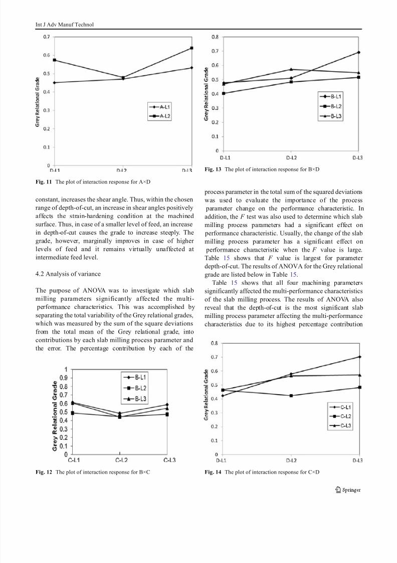
Figure 13 exhibits a strong interaction effect of cutting

speed and depth-of-cut on the Grey relational grade. The

increase in surface residual strain and surface roughness

during increase in the depth coupled with the higher levels

of machining speed gets compounded and consequently the

Grey grade reduces. Machining at lower speed and at

higher values of the depth-of-cut causes increase in shear

angle, which consequently reduces the residual stresses.Thus, an improvement in Grey relational grade is seen on

increase in depth-of-cut when machining is done at lower

levels of speed.

Figure 14 displays a strong interaction effect of feed and

depth-of-cut on the Grey relational grade. The grade

remains virtually unaffected with respect to increase in

depth-of-cut at intermediate feed. At lower feed, a

continuous increase in grade is seen as depth-of-cut is

increased. The increase in grade is, however, marginal at

higher feed levels. The smaller feed gives better surface

finish but an increase in depth-of-cut, keeping the feed

Fig. 10 The plot of interaction response for A×C

Fig. 9 The plot of interaction response for A×B

Table 14 Interaction response for C×D

C × D C — L1 C — L2 C — L3

D — L1 0.4224 0.4632 0.4647

D — L2 0.5796 0.4234 0.5654

D — L3 0.7031 0.4829 0.5716

Table 13 Interaction response for B×D

B× D B — L1 B — L2 B — L3

D — L1 0.4773 0.4032 0.4698

D — L2 0.5115 0.4838 0.5731

D — L3 0.6921 0.5165 0.5489




constant, increases the shear angle. Thus, within the chosen

range of depth-of-cut, an increase in shear angles positively

affects the strain-hardening condition at the machined

surface. Thus, in case of a smaller level of feed, an increase

in depth-of-cut causes the grade to increase steeply. The

grade, however, marginally improves in case of higher

levels of feed and it remains virtually unaffected at

intermediate feed level.

4.2 Analysis of variance

The purpose of ANOVA was to investigate which slab

milling parameters significantly affected the multi-

performance characteristics. This was accomplished by

separating the total variability of the Grey relational grades,

which was measured by the sum of the square deviations

from the total mean of the Grey relational grade, into

contributions by each slab milling process parameter and

the error. The percentage contribution by each of the

process parameter in the total sum of the squared deviations

was used to evaluate the importance of the process

parameter change on the performance characteristic. In

addition, the F test was also used to determine which slab

milling process parameters had a significant effect on

performance characteristic. Usually, the change of the slab

milling process parameter has a significant effect on

performance characteristic when the F value is large.

Table 15 shows that F value is largest for parameter

depth-of-cut. The results of ANOVA for the Grey relational

grade are listed below in Table 15.

Table 15 shows that all four machining parameters

significantly affected the multi-performance characteristics

of the slab milling process. The results of ANOVA also

reveal that the depth-of-cut is the most significant slab

milling process parameter affecting the multi-performance

characteristics due to its highest percentage contribution

Fig. 14 The plot of interaction response for C×D

Fig. 13 The plot of interaction response for B×D

Fig. 12 The plot of interaction response for B×C

Fig. 11 The plot of interaction response for A×D




amongst the selected process parameters. Table 9 further

shows that the percentage contribution of other parameters

in decreasing order is feed (24.01%), cutting speed

(16.29%) and cutting fluid (13.21%).

The micrographs shown in Fig. 6 suggest that in all

cases the grains have been elongated in the direction of

machining. It also appears that in all such experimental

conditions where cutting fluid was not applied (experi-ment numbers 5 to 9) and cutting speed, depth-of-cut and

feed are relatively higher, the strain is less and grain size is

large. It may be inferred that dynamic strain relieving

occurred in all such cases. Further, when the cutting fluid

was used at a relatively higher speed the temperature rose

quickly, but due to the cooling effect of the cutting fluid

the temperature decreased rapidly. This might have caused

lower strains and formation of small-sized elongated

grains. Such conditions are observed in experimental

conditions 16 to 18.

4.3 Confirmation test

After obtaining the optimal level of the slab milling process

parameters, the next step is to verify the percentage change

of Grey relational grade between predicted and experimental

values for the optimal combination. Table 16 compares the

results of the confirmation experiments using the optimal

slab milling process parameters ( A2 B1C 1 D3) obtained by the

proposed method.

As shown in Table 10, that Grey relational grade

improved from 0.7100 to 0.7623 (an improvement of

7.36%), which shows that optimal combination of the slab

milling process parameters is good enough to meet the

requirement.

5 Conclusion

This paper has presented an effective approach for theoptimization of the slab milling process of HSLA steel

with multi-performance characteristics based on the

combined Taguchi method and Grey relational analysis.

Based on the results of the present study, the following

conclusions are drawn:

& The optimum combination of slab milling parameters

and their levels for the optimum multi-performance

characteristics of the slab milling process are A2 B1C 1 D3

(i.e. cutting fluid — present, cutting speed — 1,800 r.p.m.,

feed — 150 mm/min and depth-of-cut — 0.23 mm).

& All four machining parameters, i.e. cutting fluid,

cutting speed, feed and depth-of-cut, significantly

affect the multi-performance characteristics of the

slab milling process investigated in this study. The

percent contributions of depth-of-cut, feed, cutting

speed and cutting fluid are 33.76, 24.01, 16.29 and

13.21, respectively.

& An improvement of 7.36% in the multi-performance

characteristics, i.e. Grey relational grade, was achieved

through this approach.

& The grains get elongated in the direction of machining.

The grain growth is restricted owing to the use of

cutting fluid as it reduces the after effects of heat

produced during machining.

& The absence of cutting fluid during machining leads to

grain growth due to prevailing higher temperature

during machining, which indeed alters the surface

microstructure.

& The interactions between cutting fluid and feed ( A×C ),

cutting speed and feed ( B ×C ), cutting speed and depth-

of-cut ( B× D) and feed and depth-of-cut (C × D) signifi-

cantly affect the multi-performance characteristic, i.e.

Grey relational grade.

Table 15 Results of the analysis of variance

Symbol Machining parameters Degrees of freedom Sum of square Mean square F ratio P -value Contribution (%)

A Cutting fluid 1 0.0217 0.0217 10.38 0.0091 13.21

B Cutting speed 2 0.0267 0.0134 6.40 0.0162 16.29

C Feed 2 0.0394 0.0197 9.43 0.005 24.02

D Depth of cut 2 0.0554 0.0277 13.26 0.0015 33.76

Error 10 0.0209 0.0021 12.73

Total 17 0.1641 100.00

Table 16 Results of confirmation test

Optimal machining parameters

Prediction Experiment % improvement

Level A2 B1C 1 D3 A2 B1C 1 D3

Surface roughness 1.0000

Shear strain 0.4640

Micro-hardness 0.8228

Grey relational grade 0.7100 0.7623 7.36




References

1. Field M, Kahles J (1971) Review of surface integrity of machined

components. Ann CIRP 20(2):153 – 163

2. Sun J, Guo YB (2009) A comprehensive experimental study on

surface integrity by end milling Ti – 6Al – 4V. J Mater Process

Technol 41(12):1705 – 1719

3. El-Gallab M, Sklad M (1998) Machining of Al/SiC particulate

metal matrix composites: part II: workpiece surface integrity. JMater Process Technol 209(8):4036 – 4042

4. El-Khabeery MM, El-Axir MH (2001) Experimental techniques

for studying the effects of milling roller-burnishing parameters on

surface integrity. Int J Mach Tool Manuf 41(12):1705 – 1719

5. Che-Haron CH (2001) Tool life and surface integrity in turning

titanium alloy. J Mater Process Technol 118(1 – 3):231 – 237

6. Axinte DA, Dewes RC (2002) Surface integrity of hot work tool

steel after high speed milling — experimental data and empirical

models. J Mater Process Technol 127(3):325 – 335

7. Dhar NR, Paul S, Chattopadhayay AB (2002) Machining of AISI

4140 steel under cryogenic cooling — tool wear, surface roughness

and dimensional deviation. J Mater Proc Technol 123(3):483 – 489

8. Novovic D, Dewes RC, Aspinwall DK, Voice W, Bowen P (2004)

The effect of machined topography and surface integrity on

fatigue life. Int J Mach Tool Manuf 44(2 – 3):125 – 1349. Dhar NR, Kamruzzaman M, Mahiuddin A (2006) Effect of

minimum quantity lubrication (MQL) on tool wear and surface

roughness in turning AISI-4340 steel. J Mater Process Technol

172(2):299 – 304

10. Basavarajappa S, Chandramohan G, Prabu M, Mukund K,

Ashwin M (2007) Drilling of hybrid metal matrix composites —

workpiece surface integrity. Int J Mach Tool Manuf 47(1):92 – 96

11. Javidi A, Rieger U, Eichlseder W (2008) The effect of machining

on the surface integrity and fatigue life. Intern J Fatigue 30

(10 – 11):2050 – 2055

12. Ross PJ (1988) Taguchi techniques for quality engineering.

McGraw-Hill, New York 13. Siddiquee AN, Khan ZA, Mallick Z (2010) Grey relational

analysis coupled with principal component analysis for optimization

design of the process parameters in in-feed centreless cylindrical. Int

J Adv Manuf Technol 46:983 – 992

14. Khan ZA, Kamaruddin S, Siddiquee AN (2010) Feasibility study

of use of recycled high density polyethylene and multi response

optimization of injection moulding parameters using combined

Grey relational and principal component analyses. Mater Des

31:2925 – 2931

15. Yang YY, Shie JR, Huang CH (2006) Optimization of dry

machining parameters for high purity graphite in end-milling

process. Mater Manuf Process 21:832 – 837

16. Phadke SM (1989) Quality engineering using robust design.

Prentice-Hall, New York

17. Unal R, Stanley DO, Joyner CR (1993) Propulsion system designoptimization using the Taguchi method. IEEE Trans Eng Manag

40:315 – 322


Influence of Slab Milling Process Parameters on Surface Integrity of HSLA- A Multi-performance...

Documents

Transcript of Influence of Slab Milling Process Parameters on Surface Integrity of HSLA- A Multi-performance...