Influence of ozone recovery and greenhouse gas increases...

Influence of ozone recovery and greenhouse gas increaseson Southern Hemisphere circulation

Alexey Y. Karpechko,1,2 Nathan P. Gillett,3 Lesley J. Gray,4 and Mauro Dall’Amico5,6

Received 27 April 2010; revised 6 September 2010; accepted 13 September 2010; published 24 November 2010.

[1] Stratospheric ozone depletion has significantly influenced the tropospheric circulationand climate of the Southern Hemisphere (SH) over recent decades, the largest trendsbeing detected in summer. These circulation changes include acceleration of theextratropical tropospheric westerly jet on its poleward side and lowered Antarctic sea levelpressure. It is therefore expected that ozone changes will continue to influence climateduring the 21st century when ozone recovery is expected. Here we use two contrastingfuture ozone projections from two chemistry‐climate models (CCMs) to force 21st centurysimulations of the HadGEM1 coupled atmosphere‐ocean model, along with A1Bgreenhouse gas (GHG) concentrations, and study the simulated response in the SHcirculation. According to several studies, HadGEM1 simulates present troposphericclimate better than the majority of other available models. When forced by the larger ozonerecovery trends, HadGEM1 simulates significant deceleration of the tropospheric jet on itspoleward side in the upper troposphere in summer, but the trends in the lower troposphereare not significant. In the simulations with the smaller ozone recovery trends the zonalmean zonal wind trends are not significant throughout the troposphere. The response of theSH circulation to GHG concentration increases in HadGEM1 includes an increase inpoleward eddy heat flux in the stratosphere and positive sea level pressure trends insoutheastern Pacific. The HadGEM1‐simulated zonal wind trends are considerablysmaller than the trends simulated by the CCMs, both in the stratosphere and inthe troposphere, despite the fact that the zonal mean ozone trends are thesame between these simulations.

Citation: Karpechko, A. Y., N. P. Gillett, L. J. Gray, and M. Dall’Amico (2010), Influence of ozone recovery and greenhousegas increases on Southern Hemisphere circulation, J. Geophys. Res., 115, D22117, doi:10.1029/2010JD014423.

1. Introduction

[2] Antarctic stratospheric ozone depletion caused byanthropogenic halogens significantly contributed to theobserved acceleration of the Southern Hemisphere (SH)extratropical tropospheric westerly jet on its poleward sideduring the last decades of the 20th century [Kindem andChristiansen, 2001; Sexton, 2001; Gillett and Thompson,2003]. As the release of the ozone depleting substances(ODSs) to the atmosphere slowed following the Montrealprotocol, their atmospheric concentration has started to

decline [World Meteorological Organization (WMO),2007]. It is expected that the removal of anthropogenicODSs from the atmosphere will lead to the recovery ofstratospheric ozone layer by the mid‐21st century [e.g.,Eyring et al., 2007]. The beginning of ozone recovery mayalready have been detected [e.g., Stolarski and Frith, 2006].[3] Whether or not ozone recovery will be followed by the

reversal of the tropospheric circulation changes remains anopen question. Fyfe et al. [1999] and Kushner et al. [2001]showed that the increase of greenhouse gas (GHG) concen-tration, which is expected to continue throughout the 21stcentury, can lead to an acceleration of the SH troposphericjet and an accompanied positive trend of the SouthernAnnular Mode (SAM). While during the 20th century bothGHG concentration increase and ozone depletion forced thecirculation toward a more positive SAM, their effects duringthe period of ozone recovery will compete with each other.The matter is complicated by the fact that changes in strato-spheric temperature and dynamics related to the GHG con-centration increases will influence the ozone evolution, andozone concentrations may not be the same as in the preozonehole period even when the anthropogenic ODSs have beenremoved from the atmosphere [Waugh et al., 2009a].

1Climatic Research Unit, School of Environmental Sciences, Universityof East Anglia, Norwich, UK.

2Now at Arctic Research Unit, Finnish Meteorological Institute,Helsinki, Finland.

3Canadian Centre for Climate Modelling and Analysis, EnvironmentCanada, Victoria, British Columbia, Canada.

4Climate Directorate, National Centre for Atmospheric Sciences,Meteorology Department, University of Reading, Reading, UK.

5Deutsches Zentrum für Luft‐ und Raumfahrt, Institut für Physik derAtmosphäre, Oberpfaffenhofen, Germany.

6Now at Astrium GmbH, Ottobrunn, Germany.

Copyright 2010 by the American Geophysical Union.0148‐0227/10/2010JD014423

JOURNAL OF GEOPHYSICAL RESEARCH, VOL. 115, D22117, doi:10.1029/2010JD014423, 2010

D22117 1 of 15

http://dx.doi.org/10.1029/2010JD014423

[4] The combined effect of GHG increases and ozonerecovery on the SH circulation was first studied by Shindelland Schmidt [2004] in an atmosphere‐ocean general circu-lation model (AOGCM) with relatively coarse resolution. Intheir model the effects of ozone recovery and GHG increasesroughly balanced each other resulting in insignificant trendsin the tropospheric circulation. Further studies withAOGCMs showed significant positive trends of the SAM insummer [Arblaster and Meehl, 2006; Miller et al., 2006],suggesting a dominant influence of the GHG concentrationincrease. However, future ozone changes in some of thesemodels were obtained from simple regression modelsbased on projected ODSs concentrations [Stott et al., 2006]while some other models suffered from erroneously specifiedozone forcing [Miller et al., 2006].[5] A different perspective is given by coupled chemistry

climate models (CCMs). Some CCMs simulate a decelera-tion of the tropospheric jet stream and a negative SAM trendin summer [Perlwitz et al., 2008; Son et al., 2008, Waughet al., 2009b], although the spread across the CCMs pre-dictions is large and the most recent CCMVal‐2 simulationsshow no significant jet location trend in the summer onaverage [Baldwin et al., 2010; Son et al., 2010]. The modelsused in these studies were run with prescribed sea surfacetemperatures (SSTs), constraining the possible troposphericresponse, although Sigmond et al. [2010] did not find sig-nificant difference between the SAM response to ozonedepletion in a model forced by prescribed SSTs and a modelcoupled to a full ocean.[6] The present study is aimed at modeling the SH cir-

culation changes during the period of ozone recovery and isdesigned to overcome some of the deficiencies identified inthe previous studies. In this study we use a high‐resolutionAOGCM forced by both GHG concentration increases andozone recovery scenarios based on CCM simulations. Wechoose a model which, according to several studies, simu-lates many aspects of present tropospheric climate betterthan the majority of other available AOGCMs. The modelhas a fully coupled ocean, which means that its response toan applied forcing is not constrained by prescribed SSTs. Toaccount for uncertainties in future ozone evolution, twocontrasting ozone recovery scenarios are considered inaddition to the scenario in which no ozone recovery istaking place.

2. Model and Methods

[7] The Hadley Centre global environmental model ver-sion 1 (HadGEM1) described by Martin et al. [2006],Ringer et al. [2006], and Johns et al. [2006] is used in thisstudy. The atmospheric component of the model has hori-zontal resolution of 1.25° latitude by 1.875° longitude and38 levels from the surface to about 39 km with 16 levelstypically located above 300 hPa. The oceanic component ofthe model has a horizontal resolution of 1° (the meridionalresolution is 1° between the poles and 30° latitude, fromwhere it increases smoothly to 1/3° at the equator) and 40unevenly spaced vertical levels. Several studies [Miller et al.,2006; Connolley and Bracegirdle, 2007; Karpechko et al.,2009] have shown that HadGEM1 ranks as one of thebest AOGCMs in its simulation of global and Antarctic cli-mates, SAM spatial structure, as well as climate impacts of

the SAM across the CMIP3 models used in the IPCC AR4assessment.[8] The model is run to simulate climate change from

1 December 1978 to 1 December 2049, which comprises theperiods of ozone depletion and recovery. Simulations of thepast climate were forced by observed changes in well mixedGHGs, tropospheric and stratospheric ozone, aerosols, landuse, solar irradiance and stratospheric volcanic aerosols.Implementation of the forcing, except ozone forcing, isdescribed in detail by Stott et al. [2006]. Implementation ofozone forcing is described by Dall’Amico et al. [2010a]. Inthese simulations ozone is prescribed as zonal meanmonthly mean values based on satellite observations, insteadof the monthly climatology with an imposed linear trendcomponent, as is usually employed in AOGCM experi-ments. It therefore includes significant interannual vari-ability such as that associated with the Quasi‐BiennialOscillation (QBO) and 11 year solar cycle. The model alsoimplements a relaxation toward the observed QBO instratospheric winds. The implemented changes result insome improvements of the simulated climate variability andtrends as described by Dall’Amico et al. [2010a, 2010b].Altogether six 20 year simulations (1 December 1978 to1 December 1999), referred to as ‘Observed_O3’ experi-ments, are considered in this study, three of which are partsof the ‘baseline+ozone+QBO’ simulations discussed byDall’Amico et al. [2010a, 2010b] and another three identicalsimulations that have been conducted at a different com-puting facility. The end points of the latter three simulationsare used as starting points for the scenario simulations.[9] The scenario simulations include three main experi-

ments, each consisting of three ensemble members coveringthe period from 1 December 1999 to 1 December 2049.The experiments differ in the prescribed ozone forcing butare identical otherwise. The forcing in these experimentsincludes GHG concentration increases following the SRESA1B emission scenario and changes in aerosols and land useas described by Stott et al. [2006]. The relaxation toward theQBO is not included in these experiments. Scenario ozonefields for two of the experiments are taken from CCMsimulations which have been accomplished as a part of theChemistry‐Climate Model Validation (CCMVal‐1) activityin support of WMO ozone assessment 2006 [WMO, 2007].The CCM simulations are described in detail by Eyringet al. [2007], where they are referred to as REF2 simula-tions. Ozone outputs of two CCMs, GEOSCCM [Pawsonet al., 2008] and CMAM [Fomichev et al., 2007], areused in our experiments referred to as ‘GEOSCCM_O3’ and‘CMAM_O3’, respectively. Like all models these twoCCMs have biases; however comparison with observationsshow that these two CCMs are among the better performingmodels of those which participated in the CCMVal‐1activity [Eyring et al., 2006; Waugh and Eyring, 2008;Karpechko et al., 2010]. GEOSCCM simulates one of thelargest while CMAM simulates one of the smallest ozonetrends (negative during ozone depletion and positive duringozone recovery) across the CCMVal‐1 models [Eyringet al., 2006, 2007; Karpechko et al., 2010]. Analyzingsimulations with two contrasting ozone evolutions allowsus to better assess uncertainties in future tropospheric cli-mate changes associated with future ozone.

KARPECHKO ET AL.: OZONE RECOVERY AND SH CIRCULATION D22117D22117

2 of 15

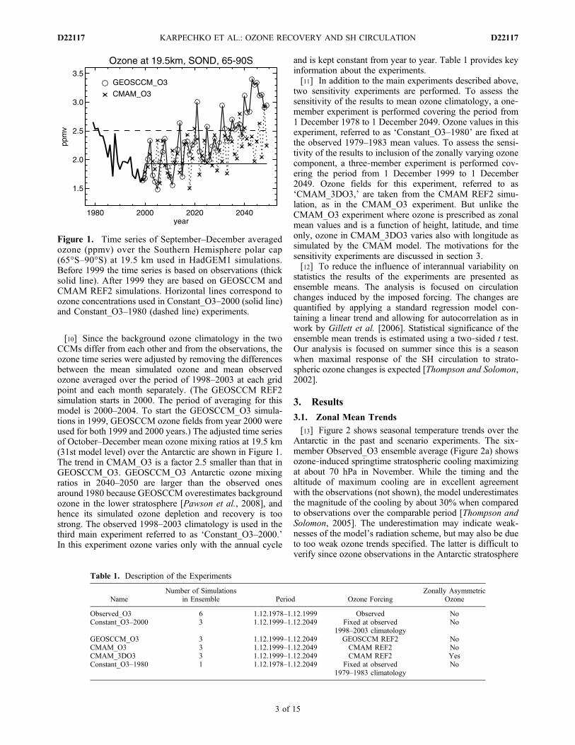
[10] Since the background ozone climatology in the twoCCMs differ from each other and from the observations, theozone time series were adjusted by removing the differencesbetween the mean simulated ozone and mean observedozone averaged over the period of 1998–2003 at each gridpoint and each month separately. (The GEOSCCM REF2simulation starts in 2000. The period of averaging for thismodel is 2000–2004. To start the GEOSCCM_O3 simula-tions in 1999, GEOSCCM ozone fields from year 2000 wereused for both 1999 and 2000 years.) The adjusted time seriesof October–December mean ozone mixing ratios at 19.5 km(31st model level) over the Antarctic are shown in Figure 1.The trend in CMAM_O3 is a factor 2.5 smaller than that inGEOSCCM_O3. GEOSCCM_O3 Antarctic ozone mixingratios in 2040–2050 are larger than the observed onesaround 1980 because GEOSCCM overestimates backgroundozone in the lower stratosphere [Pawson et al., 2008], andhence its simulated ozone depletion and recovery is toostrong. The observed 1998–2003 climatology is used in thethird main experiment referred to as ‘Constant_O3–2000.’In this experiment ozone varies only with the annual cycle

and is kept constant from year to year. Table 1 provides keyinformation about the experiments.[11] In addition to the main experiments described above,

two sensitivity experiments are performed. To assess thesensitivity of the results to mean ozone climatology, a one‐member experiment is performed covering the period from1 December 1978 to 1 December 2049. Ozone values in thisexperiment, referred to as ‘Constant_O3–1980’ are fixed atthe observed 1979–1983 mean values. To assess the sensi-tivity of the results to inclusion of the zonally varying ozonecomponent, a three‐member experiment is performed cov-ering the period from 1 December 1999 to 1 December2049. Ozone fields for this experiment, referred to as‘CMAM_3DO3,’ are taken from the CMAM REF2 simu-lation, as in the CMAM_O3 experiment. But unlike theCMAM_O3 experiment where ozone is prescribed as zonalmean values and is a function of height, latitude, and timeonly, ozone in CMAM_3DO3 varies also with longitude assimulated by the CMAM model. The motivations for thesensitivity experiments are discussed in section 3.[12] To reduce the influence of interannual variability on

statistics the results of the experiments are presented asensemble means. The analysis is focused on circulationchanges induced by the imposed forcing. The changes arequantified by applying a standard regression model con-taining a linear trend and allowing for autocorrelation as inwork by Gillett et al. [2006]. Statistical significance of theensemble mean trends is estimated using a two‐sided t test.Our analysis is focused on summer since this is a seasonwhen maximal response of the SH circulation to strato-spheric ozone changes is expected [Thompson and Solomon,2002].

3. Results

3.1. Zonal Mean Trends

[13] Figure 2 shows seasonal temperature trends over theAntarctic in the past and scenario experiments. The six‐member Observed_O3 ensemble average (Figure 2a) showsozone‐induced springtime stratospheric cooling maximizingat about 70 hPa in November. While the timing and thealtitude of maximum cooling are in excellent agreementwith the observations (not shown), the model underestimatesthe magnitude of the cooling by about 30% when comparedto observations over the comparable period [Thompson andSolomon, 2005]. The underestimation may indicate weak-nesses of the model’s radiation scheme, but may also be dueto too weak ozone trends specified. The latter is difficult toverify since ozone observations in the Antarctic stratosphere

Figure 1. Time series of September–December averagedozone (ppmv) over the Southern Hemisphere polar cap(65°S–90°S) at 19.5 km used in HadGEM1 simulations.Before 1999 the time series is based on observations (thicksolid line). After 1999 they are based on GEOSCCM andCMAM REF2 simulations. Horizontal lines correspond toozone concentrations used in Constant_O3–2000 (solid line)and Constant_O3–1980 (dashed line) experiments.

Table 1. Description of the Experiments

NameNumber of Simulations

in Ensemble Period Ozone ForcingZonally Asymmetric

Ozone

Observed_O3 6 1.12.1978–1.12.1999 Observed NoConstant_O3–2000 3 1.12.1999–1.12.2049 Fixed at observed

1998–2003 climatologyNo

GEOSCCM_O3 3 1.12.1999–1.12.2049 GEOSCCM REF2 NoCMAM_O3 3 1.12.1999–1.12.2049 CMAM REF2 NoCMAM_3DO3 3 1.12.1999–1.12.2049 CMAM REF2 YesConstant_O3–1980 1 1.12.1978–1.12.2049 Fixed at observed

1979–1983 climatologyNo


3 of 15

are scarce, which explains why Antarctic ozone trends inobservation‐based data sets differ significantly [Karpechkoet al., 2010]. The data set employed in this study showsthe smallest ozone trends during austral spring across thethree data sets analyzed by Karpechko et al. [2010]. Whenforced by an ozone data set with larger ozone trends[Dall’Amico et al., 2010a, 2010b], HadGEM1 simulatescooling that is in a good agreement with observations(not shown).[14] The scenario simulations forced by ozone recovery

scenarios reveal warming of the lower stratosphere with amaximum at 100 hPa in December (Figures 2b and 2c).Consistent with the larger ozone trends in the GEOSCCM_O3simulations, the warming is larger in these simulations thanin CMAM_O3. The ratio of warming in GEOSCCM_O3 tothat in CMAM_O3 is close to the ratio of the correspondingozone trends. Statistically significant warming in the lowerstratosphere in November–January is also simulated in theConstant_O3–2000 experiment, which is somewhat surpris-ing, given the constant ozone forcing in these simulations. Aswill be shown below this warming is attributable to thedynamical heating caused by increased planetary wave prop-agation into the stratosphere associated with increases inGHG concentrations.[15] Figure 3 shows the zonal mean zonal wind trends

in the SH in the past and scenario experiments averagedover December–February. The Observed_O3 simulations(Figure 3a) reproduce the strengthening of the stratosphericwinds and the acceleration of the tropospheric jet stream onthe polarward side seen in the ERA‐40 reanalysis data [Son

et al., 2008], although with a smaller magnitude thanobserved, which is, at least partly, due to the under-estimated stratospheric cooling. The poleward shift of thetropospheric jet stream is consistent with a positive SAMtrend. Positive trends are also simulated equatorward of40°S both in the stratosphere and in the troposphere, whichare not seen in the ERA‐40 reanalysis [Son et al., 2008].[16] Both ozone recovery experiments reveal a weakening

of the stratospheric winds, but this is only significant inGEOSCCM_O3 (Figures 3b and 3c). GEOSCCM_O3 showsan equatorward shift of the tropospheric jet stream at 50°S,with the negative trends at 60°S extending to the surface butnot statistically significant below 400 hPa. The jet streamshift is not simulated in CMAM_O3. Significant negativetrends in polar stratospheric winds are simulated in Con-stant_O3–2000 (Figure 3d), which is consistent with thelower stratospheric warming in these simulations. There isalso an insignificant deceleration of the tropospheric jet onthe poleward side in Constant_O3–2000. The opposite windtrends in the subtropical stratosphere between Con-stant_O3_2000 and the ozone recovery experiments may beattributed, at least partly, to differential meridional heatingdue to ozone trends in the ozone recovery experiments,where ozone recovery in the midlatitude stratosphere anda weak ozone depletion in the tropical stratosphere (likelydue to intensified meridional circulation in the CCM simu-lations, not shown) result in an easterly thermal wind trendin the subtropical stratosphere.[17] Based on previous studies [Miller et al., 2006; Son

et al., 2008] it was expected that, in the absence of ozone

Figure 2. Seasonal cycle of linear trends in temperature (K per decade) over the Southern Hemispherepolar cap (65°S–90°S) in (a) Observed_O3, (b) GEOSCCM_O3, (c) CMAM_O3, and (d) Constant_O3–2000 experiments. Shading denotes trends significant at the 5% level allowing for autocorrelation.


4 of 15

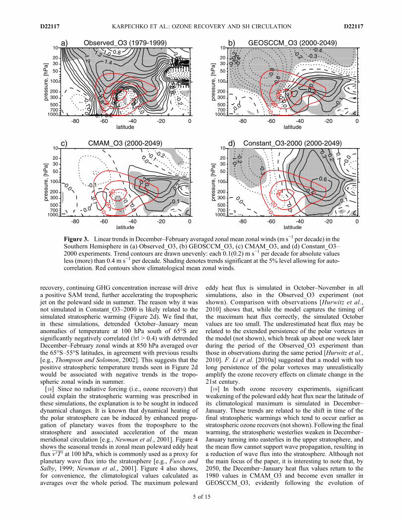
recovery, continuing GHG concentration increase will drivea positive SAM trend, further accelerating the troposphericjet on the poleward side in summer. The reason why it wasnot simulated in Constant_O3–2000 is likely related to thesimulated stratospheric warming (Figure 2d). We find that,in these simulations, detrended October–January meananomalies of temperature at 100 hPa south of 65°S aresignificantly negatively correlated (∣r∣ > 0.4) with detrendedDecember–February zonal winds at 850 hPa averaged overthe 65°S–55°S latitudes, in agreement with previous results[e.g., Thompson and Solomon, 2002]. This suggests that thepositive stratospheric temperature trends seen in Figure 2dwould be associated with negative trends in the tropo-spheric zonal winds in summer.[18] Since no radiative forcing (i.e., ozone recovery) that

could explain the stratospheric warming was prescribed inthese simulations, the explanation is to be sought in induceddynamical changes. It is known that dynamical heating ofthe polar stratosphere can be induced by enhanced propa-gation of planetary waves from the troposphere to thestratosphere and associated acceleration of the meanmeridional circulation [e.g., Newman et al., 2001]. Figure 4shows the seasonal trends in zonal mean poleward eddy heatflux v 0T 0 at 100 hPa, which is commonly used as a proxy forplanetary wave flux into the stratosphere [e.g., Fusco andSalby, 1999; Newman et al., 2001]. Figure 4 also shows,for convenience, the climatological values calculated asaverages over the whole period. The maximum poleward

eddy heat flux is simulated in October–November in allsimulations, also in the Observed_O3 experiment (notshown). Comparison with observations [Hurwitz et al.,2010] shows that, while the model captures the timing ofthe maximum heat flux correctly, the simulated Octobervalues are too small. The underestimated heat flux may berelated to the extended persistence of the polar vortexes inthe model (not shown), which break up about one week laterduring the period of the Observed_O3 experiment thanthose in observations during the same period [Hurwitz et al.,2010]. F. Li et al. [2010a] suggested that a model with toolong persistence of the polar vortexes may unrealisticallyamplify the ozone recovery effects on climate change in the21st century.[19] In both ozone recovery experiments, significant

weakening of the poleward eddy heat flux near the latitude ofits climatological maximum is simulated in December–January. These trends are related to the shift in time of thefinal stratospheric warmings which tend to occur earlier asstratospheric ozone recovers (not shown). Following the finalwarming, the stratospheric westerlies weaken in December–January turning into easterlies in the upper stratosphere, andthe mean flow cannot support wave propagation, resulting ina reduction of wave flux into the stratosphere. Although notthe main focus of the paper, it is interesting to note that, by2050, the December–January heat flux values return to the1980 values in CMAM_O3 and become even smaller inGEOSCCM_O3, evidently following the evolution of

Figure 3. Linear trends in December–February averaged zonal mean zonal winds (m s−1 per decade) in theSouthern Hemisphere in (a) Observed_O3, (b) GEOSCCM_O3, (c) CMAM_O3, and (d) Constant_O3–2000 experiments. Trend contours are drawn unevenly: each 0.1(0.2) m s−1 per decade for absolute valuesless (more) than 0.4 m s−1 per decade. Shading denotes trends significant at the 5% level allowing for auto-correlation. Red contours show climatological mean zonal winds.


5 of 15

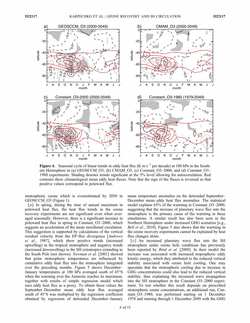
stratospheric ozone which is overestimated by 2050 inGEOSCCM_O3 (Figure 1).[20] In spring, during the time of annual maximum in

poleward heat flux, the heat flux trends in the ozonerecovery experiments are not significant even when aver-aged seasonally. However, there is a significant increase inpoleward heat flux in spring in Constant_O3–2000, whichsuggests an acceleration of the mean meridional circulation.This suggestion is supported by calculations of the verticalresidual velocity from the EP‐flux divergence [Andrewset al., 1987], which show positive trends (increasedupwelling) in the tropical stratosphere and negative trends(increased downwelling) in the SH extratropics extending tothe South Pole (not shown). Newman et al. [2001] showedthat polar stratospheric temperatures are influenced bycumulative eddy heat flux into the stratosphere integratedover the preceding months. Figure 5 shows December–January temperatures at 100 hPa averaged south of 65°Swhen the warming over the Antarctic reaches its maximum,together with results of simple regression model whichuses eddy heat flux as a proxy. To obtain these values theSeptember–December mean eddy heat flux averagedsouth of 45°S was multiplied by the regression coefficientobtained by regression of detrended December–January

mean temperature anomalies on the detrended September–December mean eddy heat flux anomalies. The statisticalmodel explains 65% of the warming in Constant_O3–2000,suggesting that the increase of planetary wave flux into thestratosphere is the primary cause of the warming in thesesimulations. A similar result has also been seen in theNorthern Hemisphere under increased GHG scenarios [e.g.,Bell et al., 2010]. Figure 5 also shows that the warming inthe ozone recovery experiments cannot be explained by heatflux changes alone.[21] An increased planetary wave flux into the SH

stratosphere under ozone hole conditions has previouslybeen reported by Rind et al. [2009]. In their model theincrease was associated with increased tropospheric eddykinetic energy, which they attributed to the reduced verticalstability associated with ozone hole cooling. One mayspeculate that the stratospheric cooling due to increase inGHG concentrations could also lead to the reduced verticalstability, thus explaining the increased wave propagationinto the SH stratosphere in the Constant_O3–2000 experi-ment. To test whether this result depends on prescribedstratospheric ozone concentrations, an additional run, Con-stant_O3–1980, was performed starting on 1 December1978 and running through 1 December 2049 with the GHG

Figure 4. Seasonal cycle of linear trends in eddy heat flux (K m s−1 per decade) at 100 hPa in the South-ern Hemisphere in (a) GEOSCCM_O3, (b) CMAM_O3, (c) Constant_O3–2000, and (d) Constant_O3–1980 experiments. Shading denotes trends significant at the 5% level allowing for autocorrelation. Redcontours show climatological mean eddy heat fluxes. Note that the sign of the fluxes is reversed so thatpositive values correspond to poleward flux.


6 of 15

forcing identical to that in the past and scenario simulationsdescribed above but with ozone concentrations fixed at1979–1983 mean values (see Figure 1). Figure 4d showsthat in Constant_O3–1980 there are positive poleward heatflux trends between August and December with magnitudessomewhat lower than those in the Constant_O3–2000ensemble mean. The heat flux trend in Constant_O3–1980 isstatistically significant at the 5% level when averaged overSeptember–December (Figure 5d). The result suggests thatthe increase in SH polarward heat flux is a robust responseto increased GHG concentrations in HadGEM‐1. Themagnitude of the heat flux trend in Constant_O3–1980 isonly half of the ensemble mean trend in Constant_O3–2000,but one of the three Constant_O3–2000 ensemble membersshows a trend of comparable magnitude to that in Con-stant_O3–1980. Therefore the statistics does not allow usto conclude whether or not the eddy heat flux increasedepends on stratospheric ozone concentration. Consistentwith the heat flux trend, a lower stratosphere warmingis observed in Constant_O3–1980 in late spring andearly summer peaking at 0.3K per decade at 100 hPain November, although it is not statistically significant ineither month.

3.2. Surface Trends

[22] Marshall [2003] reported a significant positive trendin the SAM in the late 20th century associated with loweredmean sea level pressure (MSLP) over the Antarctic andincreased MSLP in midlatitudes. Figure 6 shows mean sealevel pressure trends in the past and scenario simulationsaveraged over December–February. In the Observed_O3experiment, MSLP decreases over high latitudes (south of55°S) and increases in the midlatitude belt strongly projecton the positive SAM phase, consistent with observations.The scenario experiments (Figures 6b–6d) reveal littleannular component, consistent with the absence of signifi-cant zonal wind trends near the surface (Figures 3b–3d).Figure 6 shows a strong nonannular component of the futuretrends in high latitudes dominated by positive pressuretrends centered in the southeastern Pacific, north of theAmundsen and Bellingshausen Seas (ABS).[23] Neff et al. [2008] and Turner et al. [2009] recently

showed that the response of circulation to ozone depletionincludes a zonally asymmetric component. Turner et al.[2009] found a significant decrease of geopotential heightat 500 hPa in austral autumn centered in the southeastern

Figure 5. Time series of December–January averaged temperature over the Southern Hemispherepolar cap (65°S–90°S, solid lines) and synthetic temperature based on regression on September–December eddy heat flux averaged over 45°S–90°S (dotted lines) in (a) GEOSCCM_O3, (b) CMAM_O3,(c) Constant_O3–2000, and (d) Constant_O3–1980 experiments. Straight lines show linear trend fits.


7 of 15

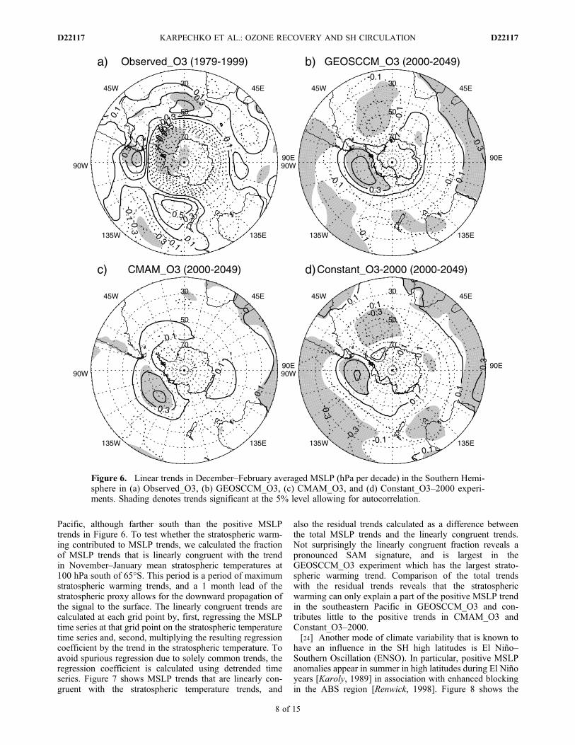
Pacific, although farther south than the positive MSLPtrends in Figure 6. To test whether the stratospheric warm-ing contributed to MSLP trends, we calculated the fractionof MSLP trends that is linearly congruent with the trendin November–January mean stratospheric temperatures at100 hPa south of 65°S. This period is a period of maximumstratospheric warming trends, and a 1 month lead of thestratospheric proxy allows for the downward propagation ofthe signal to the surface. The linearly congruent trends arecalculated at each grid point by, first, regressing the MSLPtime series at that grid point on the stratospheric temperaturetime series and, second, multiplying the resulting regressioncoefficient by the trend in the stratospheric temperature. Toavoid spurious regression due to solely common trends, theregression coefficient is calculated using detrended timeseries. Figure 7 shows MSLP trends that are linearly con-gruent with the stratospheric temperature trends, and

also the residual trends calculated as a difference betweenthe total MSLP trends and the linearly congruent trends.Not surprisingly the linearly congruent fraction reveals apronounced SAM signature, and is largest in theGEOSCCM_O3 experiment which has the largest strato-spheric warming trend. Comparison of the total trendswith the residual trends reveals that the stratosphericwarming can only explain a part of the positive MSLP trendin the southeastern Pacific in GEOSCCM_O3 and con-tributes little to the positive trends in CMAM_O3 andConstant_O3–2000.[24] Another mode of climate variability that is known to

have an influence in the SH high latitudes is El Niño–Southern Oscillation (ENSO). In particular, positive MSLPanomalies appear in summer in high latitudes during El Niñoyears [Karoly, 1989] in association with enhanced blockingin the ABS region [Renwick, 1998]. Figure 8 shows the

Figure 6. Linear trends in December–February averaged MSLP (hPa per decade) in the Southern Hemi-sphere in (a) Observed_O3, (b) GEOSCCM_O3, (c) CMAM_O3, and (d) Constant_O3–2000 experi-ments. Shading denotes trends significant at the 5% level allowing for autocorrelation.


8 of 15

trends that are linearly congruent with the El Niño 3.4 indexused as a proxy of ENSO variability, and the residual trends.In high latitudes, the linearly congruent fraction includespositive trends in the southeastern Pacific, which resemblethe total trend patterns and the residual trends in this regionare insignificant. We also note that SSTs in the El Niño 3.4index increase at a similar rate across the experiments.[25] The link between tropical SSTs and the extratropical

circulation anomalies is however complicated. Several au-thors [e.g., Harangozo, 2004; Grassi et al., 2009] showedthat the regions of anomalous convection, which triggers theteleconnection pattern in the extratropics by exciting plan-etary Rossby waves, may not coincide with the area ofstrongest SST anomalies. S. Li et al. [2010] demonstratedthat a teleconnection pattern linking tropical Pacific with theextratropics may be triggered by a warming of the tropicalIndian Ocean. They speculated that the response in thePacific may be associated with the Walker cell anomalylinked to the Indian Ocean forcing. Consistent with thefindings by S. Li et al. [2010], we find that a patternessentially similar to that shown in Figure 8 can be obtainedusing the Indian Ocean SSTs averaged over the area used byS. Li et al. [2010] (5°S to 5°N, 40°E to 110°E), instead ofthe El Nino 3.4 index (not shown). Our results thereforestrongly suggest that the warming of the tropical oceanscontributed to the MSLP changes in high latitudes seen in

Figure 6; however it is not possible within our experimentsto attribute the extratropical changes to warming in a spe-cific tropical region.[26] Figure 9 shows comparison of the December–

February SAM index evolution in our experiments to thatin the multimodel CMIP3 database [Miller et al., 2006; Sonet al., 2008]. Following Miller et al. [2006] the SAM isdefined as the first empirical orthogonal function of MSLPand the SAM index is defined as projection of MSLP onthe SAM. The anomalies are calculated with respect to theperiod 1995–2005, which facilitates comparison of theindexes during the 21st century. Figure 9 shows that ourozone recovery simulations agree well with the CMIP3simulations, suggesting that the carefully chosen ozoneforcing in our experiments does not make a big difference forsimulation of the future SAM relative to the previousAOGCM simulations discussed by Son et al. [2008]. On theother hand, the Constant_O3_2000 ensemble mean divergessignificantly from the corresponding CMIP3 ensemble,which we attribute to the simulated stratospheric dynamicalwarming in Constant_O3_2000 (see section 3.1).[27] Raphael [2003] reported a significant influence of

Antarctic sea ice on the SAM in austral summer; therefore itis also necessary to discuss the evolution of sea ice. Inour experiments, December–February mean sea ice areadecreases at the average rate of 0.38 × 106 km2 per decade,

Figure 7. (a, b, c) Trends in December–February averaged MSLP (hPa per decade) in the SouthernHemisphere that are linearly congruent with November–January averaged polar cap temperaturetrends at 100 hPa and (d, e, f) the residual trends calculated as a difference between the total trends(Figures 6b–6d) and the linearly congruent trends in GEOSCCM_O3 (Figures 7a and 7d), CMAM_O3(Figures 7b and 7e), and Constant_O3–2000 (Figures 7c and 7f) experiments. Shading in Figures 7d–7fdenotes trends significant at the 5% level allowing for autocorrelation.


9 of 15

Figure 8. (a, b, c) Trends in December–February averaged MSLP (hPa per decade) in the SouthernHemisphere that are linearly congruent with December–February averaged El Niño 3.4 index trendsand (d, e, f) the residual trends calculated as a difference between the total trends (Figures 6b–6d) andthe linearly congruent trends in GEOSCCM_O3 (Figures 8a and 8d), CMAM_O3 (Figures 8b and 8e),and Constant_O3–2000 (Figures 8c and 8f) experiments. Shading in Figures 8d–8f denotes trendssignificant at the 5% level allowing for autocorrelation.

Figure 9. Time series of December–February averaged SAM index (hPa) in the HadGEM1 simulationspresented in this paper and in the CMIP‐3 multimodel data sets. Shown are anomalies with respect to theperiod of 1995–2005. (a) CMIP3 models that have no ozone recovery and Constant_O3_2000. (b) CMIP3models that have ozone recovery, GEOSCCM_O3, and CMAM_O3. Three members of the Observed_O3ensemble that were continued in the 21st century are shown for convenience in Figures 9a and 9b. Thickblack lines show multimodel mean index averaged across individual CMIP3 models; shaded area shows 5to 95% interval across individual CMIP3 simulations. Individual HadGEM1 simulations are shown withthin red lines, and their average is shown with thick red lines.


10 of 15

consistently across the experiments, and constitutes, by theend of the simulations, ∼87% of the values at the begin-ning of the 21st century. According to Raphael [2003], a3% decrease in the sea ice area is sufficient to induce asignificant SAM index increase; therefore the effects of thefuture decreased sea ice oppose to the influence of ozonerecovery. However, the lack of positive SAM response inConstant_O3_2000 suggests that the sea ice evolution isnot a major driver of the SAM in our experiments.

3.3. Comparison With CCM Simulations

[28] Previous studies showed that while CCMs simulate asignificant westerly jet deceleration throughout the tropo-sphere as a response to ozone recovery, AOGCMs typicallysimulate weaker zonal wind trends that do not reach thesurface [Perlwitz et al., 2008; Son et al., 2008]. There areseveral structural differences between CCMs and AOGCMs.While CCMs include coupled interactive chemistry andextend to the mesosphere or above, thus fully resolving thestratosphere, they generally impose SSTs at the lowerboundary. AOGCMs, on the other hand, have a fully cou-pled ocean but no interactive chemistry and do not fullyresolve the stratosphere. Differences in their responses aretherefore difficult to attribute. However, one reason for thedifference that can be investigated in these simulationsmight be that the ozone trends in CCMs and in AOGCMsare different. Figure 10 shows seasonal trends in SH polar

cap temperatures and December–February averaged trendsin SH zonal wind for GEOSCCM and CMAM simulationsthat provided the ozone fields used in the HadGEM1GEOSCCM_O3 and CMAM_O3 experiments correspond-ingly. Despite identical zonal mean ozone trends the CCMssimulate larger stratospheric warming than the correspond-ing HadGEM‐1 experiments (Figures 2b and 2c). Consis-tently, both CCMs simulate considerably larger (by factor2–3) negative trends in the extratropical stratosphericwinds than HadGEM‐1 does (Figures 3b and 3c). CMAMdoes not simulate deceleration in the tropospheric winds,but the trends in the GEOSCCM simulation are significantand reach the surface, in contrast to the GEOSCCM_O3experiment.[29] Recently, attention was drawn to the fact that the

simulated response of atmospheric circulation is sensitiveto whether ozone is prescribed as a zonal mean or asa zonally asymmetric quantity [Gabriel et al., 2007; Crooket al., 2008; Gillett et al., 2009]. Waugh et al. [2009b]showed that a model driven by zonal mean ozone trendsunderestimates temperature and wind responses whencompared to the same model but driven by zonally asym-metric ozone trends. To test whether the differencesbetween the HadGEM‐1 experiments and the CCMs maybe explained by the lack of zonal asymmetries in ozonefields in HadGEM‐1, another experiment, CMAM_3DO3,was performed, in which HadGEM‐1 was forced by

Figure 10. (a, c) Seasonal cycle of linear trends in temperature (K per decade) over the Southern Hemi-sphere polar cap (65°S–90°S) and (b, d) linear trends in December–February averaged zonal mean zonalwinds (m s−1 per decade) in the Southern Hemisphere in GEOSCCM REF2 (Figures 10a and 10b) andCMAM REF2 (Figures 10c and 10d) simulations. Trend contours in Figures 10b and 10d are drawnunevenly: each 0.1(0.2) m s−1 per decade for absolute values less (more) than 0.4 m s−1 per decade. Shad-ing denotes trends significant at the 5% level allowing for autocorrelation. Red contours in Figures 10band 10d show climatological mean zonal winds.


11 of 15

three‐dimensional (i.e., including zonal asymmetries)monthly mean ozone fields from the CMAM REF2 simula-tion. Note that zonally averaged ozone fields fromCMAM_3DO3 are identical to those in CMAM_O3. Ozonezonal asymmetry in CMAM_3DO3, as represented by thestandard deviation around zonal mean value, maximizes overthe SH polar cap in November and decreases significantlytoward the end of simulations following the ozone holerecovery. By prescribing ozone values, this experiment stillmisses possible chemistry‐climate feedbacks in the strato-sphere, which is an important difference from the study byWaugh et al. [2009a] which employed a fully coupledchemistry‐climate model. However, a qualitative agreementbetween the result by Waugh et al. [2009a] and those by

Crook et al. [2008] who, similarly to our experiment, used amodel with prescribed ozone values, justifies our approach.[30] Seasonal trends in SH polar cap temperatures and

December–February averaged zonal wind trends forCMAM_3DO3 are shown in Figure 11. These plots are verysimilar to the analogous plots for the CMAM_O3 experi-ment (Figures 2c and 3c), suggesting that the lack of ozonezonal asymmetry in the HadGEM‐1 experiments does notexplain the difference with the CCM results.

4. Discussion and Conclusions

[31] Figure 12 illustrates the relationships between lowerstratospheric ozone and temperature trends and midtropo-

Figure 11. (a) Seasonal cycle of linear trends in temperature (K per decade) over the Southern Hemi-sphere polar cap (65°S–90°S) and (b) linear trends in December–February averaged zonal mean zonalwinds (m s−1 per decade) in the Southern Hemisphere in the CMAM_3DO3 experiment. Trend contoursin Figure 11b are drawn unevenly: each 0.1 (0.2) m s−1 per decade for absolute values less (more) than0.4 m s−1 per decade. Shading denotes trends significant at the 5% level allowing for autocorrelation. Redcontours in Figure 11b show climatological mean zonal winds.

Figure 12. Scatterplots of November–January temperature trends at 100 hPa averaged south of 65°S and(left) September–December ozone mixing ratio at 19.5 km averaged south of 65°S and (right) December–February zonal wind trends at 500 hPa quantified by the difference in zonal winds at 60°S and 45°S. Neg-ative (positive) values of the wind difference denote the deceleration (acceleration) of westerlies on thepoleward side of the maximum wind. Ensemble mean values are shown with solid circles; individualmembers are shown with open circles.


12 of 15

spheric zonal wind trends across the HadGEM1 experi-ments. Despite considerable internal variability in the tro-pospheric response to the stratospheric forcing revealed bythe spread across the individual ensemble members, ourHadGEM1 simulations demonstrate sensitivity of the SHcirculation response to ozone recovery trends: larger ozonetrends induce a stronger circulation response which projectsmore strongly on the SAM, consistent with results of Sonet al. [2008]. However, even when HadGEM1 is forced byozone recovery trends that are among the largest plausibleaccording to projections by up‐to‐date CCMs, the simu-lated response in tropospheric zonal winds is not signifi-cant in the lower troposphere, in contrast to the ensemble‐mean response across seven CCMs studied by Son et al.[2008]. So in our model future SH ozone evolution doesnot appear to be very important for SH surface climatechange. Note that the latest generation of CCMs [Baldwinet al., 2010; Son et al., 2010] also does not show a sig-nificant trend in the lower tropospheric winds in the 21stcentury, in contrast to the previous assessment [Son et al.,2008], but consistent with our results.[32] Side‐by‐side comparison with CCMs that have

identical ozone trends reveals that HadGEM1 simulates aweaker response in stratospheric temperature and zonalwind than the CCMs. Several factors could be responsiblefor the difference, including a low upper boundary inHadGEM1, the lack of a dynamical ocean in the CCMs, ormore subtle differences between the models. Here we testeda possibility that the different response may be explained bythe lack of zonal asymmetries in ozone trends prescribedin HadGEM1. Contrary to several previous studies [Gabrielet al., 2007; Crook et al., 2008; Gillett et al., 2009; Waughet al., 2009b], we found that the inclusion of zonal asym-metries in ozone does not affect the model’s response. Onepossible explanation for this contradiction may be that inthis study we employed a model with a low upper boundarywhereas the above studies all used models with upperboundaries located in the mesosphere.[33] Apart from stratospheric ozone forcing other factors,

which are not considered here, can influence the troposphericresponse. Differences in the tropospheric zonal wind clima-tology between HadGEM1 and the CCMs (compare Figures 3and 10) can lead to different annular responses [Kidston andGerber, 2010; Son et al., 2010]. However, a simple linkbetween the simulated wind climatology and the annularresponse is difficult to establish in austral summer,whenmodeldifferences in the treatment of the stratosphere become moreimportant [Kidston and Gerber, 2010]. The troposphericresponsemay also be influenced by differences inmodel SSTs.However, the influence of different SSTs on the results shouldbe minimal at least in the case of GEOSCCM, since theGEOSCCM simulation is forced by SSTs from the Had-GEM1 SRES A1B experiment [Eyring et al., 2007] whichhas an SST warming pattern similar to our experiments.[34] We find that HadGEM1 simulates a significant

increase in eddy wave flux into the stratosphere in spring asa response to GHG increase similar to those seen in NHstudies [e.g., Bell et al., 2010]. The increase leads to a weaklower stratospheric warming over the SH polar cap in latespring–early summer even in simulations without ozonerecovery implying a strengthening of the stratosphericmeridional circulation in these simulations. The increase in

the wave flux is not seen in the simulations where bothozone recovery and GHG increases were prescribed. Thissuggests that the increased wave flux is associated withchanges in vertical wave propagation rather than withchanges in wave generation in the troposphere associatedwith, e.g., increased ocean‐land temperature contrast. SinceHadGEM1 does not have a well‐resolved stratosphere, thesimulated changes in the stratospheric meridional circulationshould be interpreted with caution and require further inves-tigation, especially taking into account that some models witha well‐resolved stratosphere simulate a weakened BD circu-lation in the Antarctic stratosphere as a response to GHGincreases [McLandress and Shepherd, 2009].[35] At the surface our simulations show little annular

response in MSLP but instead reveal positive trends centeredin southeastern Pacific. The trends appear in all experiments,suggesting that they are a robust response to the GHG con-centration increase in HadGEM1. While the trends might bepartly attributable to ozone‐induced stratospheric warming insome of the simulations, our results also suggest that they areconsistent with anomalies expected during El Niño eventsas a result of teleconnections. Yamaguchi and Noda [2006]demonstrated that El Niño–like changes are simulated by themajority of the CMIP3 AOGCM reviewed in the IPCC AR4assessment, including HadGEM1, during the 21st century as aresponse to GHG increase. On the other hand, DiNezio et al.[2010] argued that the projected changes in the tropicalPacific depart substantially from an ENSO analogy. Further,some studies [e.g., S. Li et al., 2010] demonstrated that theextratropical SH response may also be triggered by thewarming in the tropical Indian Ocean, consistent with ourcalculations. Whether or not the high‐latitude MSLP responseto the positive trend in the tropical SSTs is a robust responseacross AOGCM remains to be investigated. The MSLP trendsand associated circulation changes in the southeastern Pacificmay have important consequences for sea ice distribution[Stammerjohn et al., 2008; Turner et al., 2009].[36] In this study we have demonstrated the response of the

summertime SH circulation to GHG concentration increaseand realistic ozone recovery scenarios in a high‐resolutionAOGCM that was previously shown to be one of the bestacross the available AOGCM in simulating present tropo-spheric climate. One of the weaknesses of our model is a rel-atively low upper boundary (about 39 km), which potentiallymay influence the planetary wave propagation in the strato-sphere and so distort the atmospheric response to imposedozone trends.We plan to repeat these experiments with a high‐top version of the model once it becomes available.

[37] Acknowledgments. This work is supported by NERC ProjectNE/E006787/1. A.K. was also partly supported by Finnish Academythrough a personal postdoctoral grant and SAARA project. We acknowl-edge the GEOSCCM and CMAM modeling groups for making their simu-lations available for this analysis, the CCMVal activity for WCRP’sSPARC project for organizing and coordinating the model data analysisactivity, the BADC for collecting and archiving the CCMVal model output,and the Program for Climate Model Diagnosis and Intercomparison(PCMDI) and the WCRP’s Working Group on Coupled Modeling(WGCM) for their roles in making available the WCRP CMIP3 multimodeldata set. Support of this data set is provided by the Office of Science, U.S.Department of Energy. We thank David Plummer for providing 3‐D ozonefields from CMAM simulation, Karen Rosenlof for providing ozone dataset, the Met Office for use of HadGEM1, Scott Osprey, Lois Steenman‐


13 of 15

Clark, and Jeff Cole for help with running the model, and two anonymousreviewers for constructive comments.

ReferencesAndrews, D. G., J. R. Holton, and C. B. Leovy (1987), Middle AtmosphereDynamics, 489 pp., Academic, San Diego, Calif.

Arblaster, J. M., and G. A. Meehl (2006), Contributions of external for-cings to Southern Annular Mode trends, J. Clim., 19, 2896–2905,doi:10.1175/JCLI3774.1.

Baldwin, M. P., et al. (2010), Effects of the stratosphere on the troposphere,in SPARC CCMVal Report on the Evaluation of Chemistry‐ClimateModels, edited by V. Eyring, T. G. Shepherd, and D. W. Waugh, chap.10, pp. 379–412, WCRP, Geneva, Switzerland. (Available at http://www.atmosp.physics.utoronto.ca/SPARC/ccmval_final/PDFs_CCMVal%20June%2015/ch10.pdf)

Bell, C. J., L. J. Gray, and J. Kettleborough (2010), Changes in NorthernHemisphere stratospheric variability under increased CO2 concentrations,Q. J. R. Meteorol. Soc., 136, 1181–1190, doi:10.1002/qj.633.

Connolley, W. M., and T. J. Bracegirdle (2007), An Antarctic assessmentof IPCC AR4 coupled models, Geophys. Res. Lett., 34, L22505,doi:10.1029/2007GL031648.

Crook, J. A., N. P. Gillett, and S. P. E. Keeley (2008), Sensitivity of South-ern Hemisphere climate to zonal asymmetry in ozone, Geophys. Res.Lett., 35, L07806, doi:10.1029/2007GL032698.

Dall’Amico, M., L. J. Gray, K. H. Rosenlof, A. A. Scaife, K. P. Shine, andP. A. Stott (2010a), Stratospheric temperature trends: Impact of ozonevariability and the QBO, Clim. Dyn., 34, 381–398, doi:10.1007/s00382-009-0604-x.

Dall’Amico, M., P. A. Stott, A. A. Scaife, L. J. Gray, K. H. Rosenlof, andA. Y. Karpechko (2010b), Impact of stratospheric variability on troposphericclimate change, Clim. Dyn., 34, 399–417, doi:10.1007/s00382-009-0580-1.

DiNezio, P., A. Clement, and G. A. Vecchi (2010), Reconciling differing viewsof tropical Pacific climate change, Eos Trans. AGU, 91(16), 141–142,doi:10.1029/2010EO160001.

Eyring, V., et al. (2006), Assessment of temperature, trace species, andozone in chemistry‐climate model simulations of the recent past, J. Geo-phys. Res., 111, D22308, doi:10.1029/2006JD007327.

Eyring, V., et al. (2007), Multimodel projections of stratospheric ozone in the21st century, J. Geophys. Res., 112, D16303, doi:10.1029/2006JD008332.

Fomichev, V. I., et al. (2007), Response of the middle atmosphere toCO2 doubling: Results from the Canadian Middle Atmosphere Model,J. Clim., 20, 1121–1144, doi:10.1175/JCLI4030.1.

Fusco, A. C., and M. L. Salby (1999), Interannual variations of total ozoneand their relationship to variations of planetary wave activity, J. Clim.,12, 1619–1629, doi:10.1175/1520-0442(1999)012<1619:IVOTOA>2.0.CO;2.

Fyfe, J. C., G. Boer, and G. Flato (1999), The Arctic and Antarctic oscilla-tions and their projected changes under global warming, Geophys. Res.Lett., 26, 1601–1604, doi:10.1029/1999GL900317.

Gabriel, A., D. Peters, I. Kirchner, and H.‐F. Graf (2007), Effect of zonallyasymmetric ozone on stratospheric temperature and planetary wave prop-agation, Geophys. Res. Lett., 34, L06807, doi:10.1029/2006GL028998.

Gillett, N. P., and D. W. J. Thompson (2003), Simulation of recent South-ern Hemisphere climate change, Science, 302, 273–275, doi:10.1126/science.1087440.

Gillett, N. P., T. D. Kell, and P. D. Jones (2006), Regional climate impactsof the Southern Annular Mode, Geophys. Res. Lett., 33, L23704,doi:10.1029/2006GL027721.

Gillett, N. P., J. F. Scinocca, D. A. Plummer, and M. C. Reader (2009),Sensitivity of climate to dynamically consistent zonal asymmetries inozone, Geophys. Res. Lett., 36, L10809, doi:10.1029/2009GL037246.

Grassi, B., G. Redaelli, and G. Visconti (2009), Evidence for tropical SSTinfluence on Antarctic polar atmospheric dynamics, Geophys. Res. Lett.,36, L09703, doi:10.1029/2009GL038092.

Harangozo, S. A. (2004), The relationship of Pacific deep tropical convec-tion to the winter and springtime extratropical atmospheric circulation ofthe South Pacific in El Niño events, Geophys. Res. Lett., 31, L05206,doi:10.1029/2003GL018667.

Hurwitz, M. M., P. A. Newman, F. Li, L. D. Oman, O. Morgenstern,P. Braesicke, and J. A. Pyle (2010), Assessment of the breakup of the Ant-arctic polar vortex in two new chemistry‐climate models, J. Geophys.Res., 115, D07105, doi:10.1029/2009JD012788.

Johns, T. C., et al. (2006), The newHadleyCentre climatemodel (HadGEM1):Evaluation of coupled simulations, J. Clim., 19, 1327–1353, doi:10.1175/JCLI3712.1.

Karoly, D. J. (1989), Southern Hemisphere circulation features associatedwith El Niño–Southern Oscillation events, J. Clim., 2, 1239–1252,doi:10.1175/1520-0442(1989)002<1239:SHCFAW>2.0.CO;2.

Karpechko, A. Y., N. P. Gillett, G. J. Marshall, and J. A. Screen (2009),Climate impacts of the Southern Annular Mode simulated by the CMIP3models, J. Clim., 22, 3751–3768, doi:10.1175/2009JCLI2788.1.

Karpechko, A. Y., N. P. Gillett, B. Hassler, K. H. Rosenlof, and E. Rozanov(2010), Quantitative assessment of Southern Hemisphere ozone in chem-istry‐climate model simulations, Atmos. Chem. Phys., 10, 1385–1400,doi:10.5194/acp-10-1385-2010.

Kidston, J., and E. P. Gerber (2010), Intermodel variability of the polewardshift of the austral jet stream in the CMIP3 integrations linked to biases in20th century climatology, Geophys. Res. Lett., 37, L09708, doi:10.1029/2010GL042873.

Kindem, I. T., and B. Christiansen (2001), Tropospheric response to strato-spheric ozone loss, Geophys. Res. Lett., 28, 1547–1550, doi:10.1029/2000GL012552.

Kushner, P. J., I. M. Held, and T. L. Delworth (2001), Southern Hemi-sphere atmospheric circulation response to global warming, J. Clim.,14, 2238–2249, doi:10.1175/1520-0442(2001)014<0001:SHACRT>2.0.CO;2.

Li, F., P. A. Newman, and R. S. Stolarski (2010), Relationships betweenthe Brewer‐Dobson circulation and the Southern Annular Mode duringaustral summer in coupled chemistry‐climate model simulations, J. Geo-phys. Res., 115, D15106, doi:10.1029/2009JD012876.

Li, S., J. Perlwitz, M. P. Hoerling, and X. Chen (2010), Opposite annularresponses of the Northern and Southern Hemisphere to Indian Oceanwarming, J. Clim., 23, 3720–3738, doi:10.1175/2010JCLI3410.1.

Marshall, G. J. (2003), Trends in the Southern Annular Mode from obser-vations and reanalyses, J. Clim., 16, 4134–4143.

Martin, G. M., M. A. Ringer, V. D. Pope, A. Jones, C. Dearden, and T. J.Hinton (2006), The Physical properties of the atmosphere in the newHadley Centre global environmental model (HadGEM1). Part I: Modeldescription and global climatology, J. Clim., 19 , 1274–1301,doi:10.1175/JCLI3636.1.

McLandress, C., and T. G. Shepherd (2009), Simulated anthropogenicchanges in the Brewer‐Dobson circulation, including its extension tohigh latitudes, J. Clim., 22, 1516–1540, doi:10.1175/2008JCLI2679.1.

Miller, R. L., G. A. Schmidt, and D. T. Shindell (2006), Forced annularvariations in the 20th century Intergovernmental Panel on ClimateChange Fourth Assessment Report models, J. Geophys. Res., 111,D18101, doi:10.1029/2005JD006323.

Neff, W., J. Perlwitz, and M. Hoerling (2008), Observational evidence forasymmetric changes in tropospheric heights over Antarctica on decadaltime scales, Geophys. Res. Lett., 35, L18703, doi:10.1029/2008GL035074.

Newman, P. A., E. R. Nash, and J. E. Rosenfield (2001), What controls thetemperature of the Arctic stratosphere during the spring?, J. Geophys.Res., 106, 19,999–20,010, doi:10.1029/2000JD000061.

Pawson, S., R. S. Stolarski, A. R. Douglass, P. A. Newman, J. E. Nielsen,S. M. Frith, and M. L. Gupta (2008), Goddard Earth Observing Systemchemistry‐climate model simulations of stratospheric ozone‐temperaturecoupling between 1950 and 2005, J. Geophys. Res., 113, D12103,doi:10.1029/2007JD009511.

Perlwitz, J., S. Pawson, R. L. Fogt, J. E. Nielsen, and W. D. Neff (2008),Impact of stratospheric ozone hole recovery on Antarctic climate, Geo-phys. Res. Lett., 35, L08714, doi:10.1029/2008GL033317.

Raphael, M. N. (2003), Impact of observed sea‐ice concentration on theSouthern Hemisphere extratropical atmospheric circulation in summer,J. Geophys. Res., 108(D22), 4687, doi:10.1029/2002JD003308.

Renwick, J. A. (1998), ENSO‐related variability in the frequency of SouthPacific blocking, Mon. Weather Rev., 126, 3117–3123, doi:10.1175/1520-0493(1998)126<3117:ERVITF>2.0.CO;2.

Rind, D., J. Jonas, S. Stammerjohn, and P. Lonergan (2009), The Antarcticozone hole and the Northern Annular Mode: A stratospheric interhemi-spheric connection, Geophys. Res. Lett., 36, L09818, doi:10.1029/2009GL037866.

Ringer, M. A., et al. (2006), The physical properties of the atmosphere inthe New Hadley Centre global atmospheric model (HadGEM1), Part II:Global variability and regional climate, J. Clim., 19, 1302–1326,doi:10.1175/JCLI3713.1.

Sexton, D. M. H. (2001), The effect of stratospheric ozone depletion onthe phase of the Antarctic Oscillation, Geophys. Res. Lett., 28(19),3697–3700, doi:10.1029/2001GL013376.

Shindell, D. T., and G. A. Schmidt (2004), Southern Hemisphere climateresponse to ozone changes and greenhouse gas increases, Geophys.Res. Lett., 31, L18209, doi:10.1029/2004GL020724.

Sigmond, M., J. C. Fyfe, and J. F. Scinocca (2010), Does the ocean impactthe atmospheric response to stratospheric ozone depletion?, Geophys.Res. Lett., 37, L12706, doi:10.1029/2010GL043773.

Son, S.‐W., L. M. Polvani, D. W. Waugh, H. Akiyoshi, R. Garcia,D. Kinnison, S. Pawson, E. Rozanov, T. G. Shepherd, and K. Shibata(2008), The impact of stratospheric ozone recovery on the Southern


14 of 15

Hemisphere westerly jet, Science, 320, 1486–1489, doi:10.1126/science.1155939.

Son, S.‐W., et al. (2010), Impact of stratospheric ozone on Southern Hemi-sphere circulation change: A multimodel assessment, J. Geophys. Res.,115, D00M07, doi:10.1029/2010JD014271.

Stammerjohn, S. E., D. G. Martinson, R. C. Smith, X. Yuan, and D. Rind(2008), Trends in Antarctic annual sea ice retreat and advance and theirrelation to El Niño–Southern Oscillation and Southern Annular Modevariability, J. Geophys. Res., 113, C03S90, doi:10.1029/2007JC004269.

Stolarski, R. S., and S. M. Frith (2006), Search for evidence of trend slow‐down in the long‐term TOMS/SBUV total ozone data record: The impor-tance of instrument drift uncertainty, Atmos. Chem. Phys., 6, 4057–4065,doi:10.5194/acp-6-4057-2006.

Stott, P. A., G. S. Jones, J. A. Lowe, P. Thorne, C. Durman, T. C. Johns,and J.‐C. Thelen (2006), Transient climate simulations with theHadGEM1 climate model: Causes of past warming and future climatechange, J. Clim., 19, 2763–2782, doi:10.1175/JCLI3731.1.

Thompson, D. W. J., and S. Solomon (2002), Interpretation of recentSouthern Hemisphere climate change, Science, 296, 895–899, doi:10.1126/science.1069270.

Thompson, D. W. J., and S. Solomon (2005), Recent stratospheric cli-mate trends: Global structure and tropospheric linkages, J. Clim., 18,4785–4795, doi:10.1175/JCLI3585.1.

Turner, J., J. C. Comiso, G. J. Marshall, T. A. Lachlan‐Cope, T. Bracegirdle,T. Maksym, M. P. Meredith, Z. Wang, and A. Orr (2009), Non‐annularatmospheric circulation change induced by stratospheric ozone depletionand its role in the recent increase of Antarctic sea ice extent,Geophys. Res.Lett., 36, L08502, doi:10.1029/2009GL037524.

Waugh, D. W., and V. Eyring (2008), Quantitative performance metrics forstratospheric‐resolving chemistry‐climate models, Atmos. Chem. Phys.,8, 5699–5713, doi:10.5194/acp-8-5699-2008.

Waugh, D. W., L. Oman, S. R. Kawa, R. S. Stolarski, S. Pawson, A. R.Douglass, P. A. Newman, and J. E. Nielsen (2009a), Impacts of climatechange on stratospheric ozone recovery, Geophys. Res. Lett., 36, L03805,doi:10.1029/2008GL036223.

Waugh, D. W., L. Oman, P. A. Newman, R. S. Stolarski, S. Pawson, J. E.Nielsen, and J. Perlwitz (2009b), Effect of zonal asymmetries in strato-spheric ozone on simulated Southern Hemisphere climate trends, Geo-phys. Res. Lett., 36, L18701, doi:10.1029/2009GL040419.

World Meteorological Organization (WMO) (2007), Scientific Assessmentof Ozone Depletion: 2006, Global Ozone Res. and Monit. Proj. Rep., 50,Geneva, Switzerland.

Yamaguchi, K., and A. Noda (2006), Global warming patterns over theNorth Pacific: ENSO vs AO, J. Meteorol. Soc. Jpn., 84, 221–241,doi:10.2151/jmsj.84.221.

M. Dall’Amico, Astrium GmbH, D‐85521, Ottobrunn, Germany.N. P. Gillett, Canadian Centre for Climate Modelling and Analysis,

Environment Canada, Victoria, BC V8W 3V6, Canada.L. J. Gray, Climate Directorate, National Centre for Atmospheric

Sciences, Meteorology Department, University of Reading, Reading RG66BB, UK.A. Y. Karpechko, Arctic Research Unit, Finnish Meteorological Institute,

PO Box 503, FI‐00101 Helsinki, Finland. ([email protected])


15 of 15

Influence of ozone recovery and greenhouse gas increases...

Documents

Transcript of Influence of ozone recovery and greenhouse gas increases...