1

Influence of Bulk Microphysics Schemes upon Weather Research and 1 Forecasting (WRF) Version 3.6.1 Nor'easter Simulations 2

Stephen D. Nicholls1,2, Steven G. Decker3, Wei-Kuo Tao1, Stephen E. Lang1,4, Jainn J. Shi1,5, and Karen I. 3 Mohr1 4 1NASA-Goddard Space Flight Center, Greenbelt, 20716, United States of America 5 2Joint Center for Earth Systems Technology, University of Maryland, Baltimore, 21250, United States of America 6 3Department of Environmental Sciences, Rutgers University, New Brunswick, 08850, United States of America 7 4Science Systems and Applications, Inc., Lanham, 20706, United States of America 8 5Goddard Earth Sciences Technology and Research, Morgan State University, 21251, United States of America 9 Correspondence to: Stephen D. Nicholls (stephen.d.nicholls@nasa.gov) 10

Abstract. This study evaluated the impact of five, single- or double- moment bulk microphysics schemes (BMPSs) on Weather 11 Research and Forecasting model (WRF) simulations of seven, intense winter time cyclones impacting the Mid-Atlantic United 12 States. Five-day long WRF simulations were initialized roughly 24 hours prior to the onset of coastal cyclogenesis off the North 13 Carolina coastline. In all, 35 model simulations (5 BMPSs and seven cases) were run and their associated microphysics-related 14 storm properties (hydrometer mixing ratios, precipitation, and radar reflectivity) were evaluated against model analysis and 15 available gridded radar and ground-based precipitation products. Inter-BMPS comparisons of column-integrated mixing ratios and 16 mixing ratio profiles reveal little variability in non-frozen hydrometeor species due to their shared programming heritage, yet their 17 assumptions concerning snow and graupel intercepts, ice supersaturation, snow and graupel density maps, and terminal velocities 18 lead to considerable variability in both simulated frozen hydrometeor species and radar reflectivity. WRF-simulated precipitation 19 fields exhibit minor spatio-temporal variability amongst BMPSs, yet their spatial extent is largely conserved. Compared to ground-20 based precipitation data, WRF-simulations demonstrate low-to-moderate (0.217–0.414) threat scores and a rainfall distribution 21 shifted toward higher values. Finally, an analysis of WRF and gridded radar reflectivity data via contoured frequency with altitude 22 (CFAD) diagrams reveals notable variability amongst BMPSs, where better performing schemes favored lower graupel mixing 23 ratios and better underlying aggregation assumptions. 24

1 Introduction 25

Bulk microphysical parameterization schemes (BMPSs), within numerical modern weather prediction models (e.g., Weather 26 Research and Forecasting model [WRF; Skamarock et al., 2008]), have become increasingly complex and computationally 27 expensive. Presently, WRF offers BMPS options varying from simplistic, warm rain physics (Kessler, 1969) to multi-phase, six-28 class, two-moment microphysics (Morrison et al., 2009). Microphysics and cumulus parameterizations drive cloud and 29 precipitation processes within WRF and similar models, which has consequences for radiation, moisture, aerosols, and other 30 simulated meteorological processes. Tao et al. (2011) highlighted the importance of BMPSs in models by summarizing more than 31 36 published, microphysics-focused studies ranging from idealized simulations to hurricanes to mid-latitude convection. More 32 recently, the observation-based studies of Stark (2012) and Ganetis and Colle (2015) investigated microphysical species variability 33 within United States (U.S.) east coast winter-time cyclones (locally called “nor’easters”) and have called for further investigation 34 into how BMPSs impact these cyclones, which motivates this nor’easter study. 35

A “nor’easter” is a large (~2000 km), mid-latitude cyclone occurring from October to April and is capable of bringing 36 punishing winds, copious precipitation, and potential coastal flooding to the Northeastern U.S. (Kocin and Uccellini 2004; Jacobs 37

https://ntrs.nasa.gov/search.jsp?R=20170003720 2020-05-12T14:00:05+00:00Z

2

et al., 2005; Ashton et al., 2008). This region is home to over 65 million people and produces 16 billion U.S. dollars of daily 38 economic output (Morath, 2016). Given its high economic output, nor’easter-related damages and disruptions can be extreme. Just 39 ten strong, December nor’easters, between 1980 and 2011, produced 29.3 billion U.S. dollars in associated damages (Smith and 40 Katz, 2013). 41

Recent nor’easter studies are scarce given the extensive research efforts of the 1980s. These historical studies addressed key 42 environmental drivers including frontogenesis and baroclinicity (Bosart, 1981; Forbes et al., 1987; Stauffer and Warner, 1987), 43 anticyclones (Uccelini and Kocin, 1987), latent heat release (Uccelini et al., 1987), and moisture transport by the low-level jet 44 (Uccellini and Kocin, 1987; Mailhot and Chouinard, 1989). Despite extensive observational analyses, little attention has been 45 given to role of BMPSs in mid-latitude winter cyclones. 46

Reisner et al. (1998) ran several Mesoscale Model Version 5 winter storm simulations with multiple BMPS options that 47 impacted the Colorado Front Range during the Winter Icing and Storms Project. Double-moment BMPSs produced more accurate 48 simulations of super cooled water and ice mixing ratios than single-moment BMPSs. However, single-moment BMPS based 49 simulations vastly improved when the snow-size distribution intercepts were derived from a diagnostic equation rather than from 50 a fixed value. 51

Wu and Pretty (2010) investigated how five, six-class BMPSs affected WRF simulations of four polar-low events (two over 52 Japan, two over the Nordic Sea). Their simulations yielded nearly identical storm tracks, but notable cloud top temperature and 53 precipitation errors. Overall, the WRF single-moment BMPS (Hong and Lim, 2006) produced marginally better cloud and 54 precipitation process simulations than those from other BMPSs. For warmer, tropical cyclones, Tao et al. (2011) investigated how 55 four, six-class BMPSs impacted WRF simulations of Hurricane Katrina. They found BMPS choice minimally impacted storm 56 track, yet sea-level pressure varied up to 50 hPa. 57

Shi et al. (2010) evaluated several WRF single-moment BMPSs during a lake-effect snow event. Simulated radar reflectively 58 and cloud top temperature validation revealed that WRF accurately simulated the onset, termination, cloud cover, and band extent 59 of a lake-effect snow event, however snowfall totals at fixed points were less accurate due to interpolation of the mesoscale grid. 60 Inter-BMPS simulation differences were small because low temperatures and weak vertical velocities prevented graupel 61 generation. Reeves and Dawson (2013) investigated WRF sensitivity to eight BMPSs during a December 2009 lake-effect snow 62 event. Simulated precipitation rates and snowfall coverage were particularly sensitive to BMPSs because vertical velocities 63 exceeded hydrometeor terminal fall speeds in half of their simulations. Vertical velocity differences were attributed to varying 64 BMPS frozen hydrometeor assumptions concerning snow density values, temperature-dependent snow-intercepts, and graupel 65 generation terms. 66

This study will evaluate WRF nor’easter simulations and their sensitivity to six- and seven-class BMPSs with a focus on 67 microphysical properties and precipitation. The remainder of this paper is divided into three sections. Section 2 explains the 68 methodology and analysis methods. Section 3 shows the results. Finally section 4 describes the conclusions, its implications, and 69 prospects for future research. 70

2 Methods 71

2.1 Study design 72

WRF version 3.6.1 (hereafter W361) solves a set of fully-compressible, non-hydrostatic, Eulerian equations in terrain-73 following coordinates (Skamarock et al., 2008). Figure 1 shows the four-domain WRF grid configuration for this study with a 45-74

3

, 15-, 5-, and 1.667-km horizontal grid spacing, respectively. Additionally, this configuration includes 61 vertical levels, a 50-hPa 75 (~20 km) model top, two-way domain feedback, and cumulus parametrization is turned off for Domains 3 and 4, which are 76 convection permitting. Notably, the location of Domain 4 adjusts for each case (Fig. 1). Global Forecasting System model 77 operational analysis (GMA) data was used for WRF boundary conditions. The above model configuration (except for the 4th 78 domain) and parameterizations are derived from Nicholls and Decker (2015). Model parameterizations include: 79

Longwave radiation: New Goddard Scheme (Chou and Suarez, 1999; Chou and Suarez, 2001) 80 Shortwave radiation: New Goddard Scheme (Chou and Suarez, 1999) 81 Surface layer: Eta similarity (Monin and Obukhov, 1954; Janjic, 2002) 82 Land surface: NOAH (Chen and Dudhia, 2001) 83 Boundary layer: Mellor-Yamada-Janjic (Mellor and Yamada 1982; Janjic 2002) 84 Cumulus parameterization: Kain-Fritsch (Kain, 2004) 85 This study investigates the seven nor’easter cases described in Table 1 and shown in Fig. 1. These cases are identical to those 86

in Nicholls and Decker (2015) and represent a small, diverse sample of nor’easter events of varying intensity and seasonal timing. 87 In Table 1, the Northeast Snowfall Impact Scale (NESIS) value serves as proxy for storm severity (1 = notable, 5 = extreme) and 88 is based upon storm duration, population impacted, area affected, and snowfall severity (Kocin and Uccellini, 2004). Early and 89 late season storms (Cases 1, 2, and 7) did not have snow and thus lack a NESIS rating. 90

Five-day, WRF model simulations for this study were initialized 24 hours prior to the first precipitation impacts in the highly 91 populated Mid-Atlantic region and prior to the onset of rapid, coastal cyclogenesis off of the North Carolina coastline. This starting 92 point provides sufficient time to establish mesoscale circulations, surface baroclinic zones, and sensible and latent heat fluxes 93 (Bosart, 1981; Uccelini and Kocin, 1987; Kuo et al., 1991; Mote et al., 1997; Kocin and Uccellini, 2004; Yao et al., 2008, Kleczek 94 et al., 2014). The first nor’easter-associated precipitation impacts are defined as the first 0.5 mm (~0.02 inch) precipitation reading 95 from the New Jersey Weather and Climate Network (D. A. Robinson, pre-print, 2005) related to the cyclone. A smaller threshold 96 was not used to avoid capturing isolated showers occurring well ahead of the primary precipitation shield. 97

To investigate BMPS influence upon W361 nor’easter simulations, five BMPS are used (Table 2). These BMPSs include 98 three, six-class, three-ice, single-moment schemes (Lin [Lin6; Lin et al., 1983; Rutledge and Hobbs, 1984], Goddard Cumulus 99 Ensemble [GCE6; Tao et al., 1989; Lang et al., 2007], and WRF single moment [WSM6; Hong and Lim 2006]), a seven-class, 100 four-ice, single-moment Goddard Cumulus Ensemble scheme (GCE7; Lang et al. 2014), and finally, the six-class, three-ice, WRF 101 double-moment scheme (WDM6; Lim and Hong 2010)). In total, 35 model simulations were completed (7 nor’easters x 5 BMPSs). 102

2.2 Evaluation and analysis techniques 103

Model evaluation efforts involved comparing WRF model output to GMA, Stage IV precipitation (StIV; Fulton et al. 1998; 104 Y. Lin and K.E. Mitchell, preprints, 2005), and Multi-Radar, Multi-Sensor (MRMS) 3D volume radar reflectivity (Zhang et al. 105 2016). GMA offers six-hourly, gridded dynamical fields, including water vapor, with global coverage. StIV is a six-hourly, 4-km 106 resolution, gridded, combined radar and rain gauge precipitation product covering the United States. Finally, MRMS is two minute, 107 1.3-km resolution, gridded 3D volume radar mosaic product derived from S- and C-band radars covering the United States and 108 Southern Canada (Zhang et al. 2016) and it is the operational successor to the National Mosaic and Multi-Sensor QPE (NMQ; 109 Zhang et al. 2011) product. Both StIV and MRMS, however are limited by the detection range of their surface-based assets. All 110 cross comparisons between WRF and these evaluation data were conducted at identical grid resolution. 111

Analysis of WRF model microphysical, precipitation, and simulated radar output was comprised of three main parts: 112 precipitable mixing ratios and domain-averaged mixing ratio profiles, simulated precipitation, and simulated radar reflectivity. 113

4

Precipitable mixing ratios are calculated for all six microphysical species (vapor, cloud ice, cloud water, snow, rain, and graupel) 114 using the equation for precipitable water: 115

𝑃𝑃𝑃𝑃𝑃𝑃 = 1𝜌𝜌𝜌𝜌 ∫ 𝑤𝑤𝑃𝑃𝑠𝑠𝑠𝑠𝑠𝑠

𝑃𝑃𝑡𝑡𝑡𝑡𝑡𝑡𝑑𝑑𝑑𝑑 (1) 116

In Eq. (1), PMR is the precipitable mixing ratio in mm, ρ is the density of water (1,000 kg m-3); g is the gravitational constant 117 (9.8 m s-2); psfc is the surface pressure (Pa), ptop is the model top pressure (Pa); w is the mixing ratio (kg kg-1); dp is the change in 118 atmospheric pressure between model levels (Pa). Only water vapor PMR’s are evaluated because all other GMA mixing ratio 119 species are nonexistent and ground and space validation microphysical data are lacking, especially over the data-poor North 120 Atlantic (Li et al., 2008; Lebsock and Su, 2014). Similarly, mixing ratio profiles will only be inter-compared amongst BMPSs 121 because satellite-derived cloud ice profile products (e.g., CloudSat 2C-ICE; Deng et al. 2013) do not directly overpass Domain 4 122 during coastal cyclogenesis for any case. WRF-simulated precipitation fields and their distribution were evaluated against StIV 123 and simulation error was quantified via bias and threat score (critical success index; Wilks, 2011) values. Finally, contoured 124 frequency with altitude diagrams (CFADs) were used to validate WRF-simulated radar reflectivity relative to MRMS similar to 125 the radar validation efforts of Yuter and Houze (1995), Lang et al. (2011) and Lang et al. (2014). A CFAD offers the advantage of 126 preserving frequency distribution information, yet is insensitive to spatio-temporal errors. Additionally, CFAD-based scores were 127 calculated for each height level and with time using Eq (2). 128

𝐶𝐶𝐶𝐶 = 1 − ∑ |𝑃𝑃𝑃𝑃𝑃𝑃𝑚𝑚−𝑃𝑃𝑃𝑃𝑃𝑃𝑡𝑡|ℎ 200

(2) 129

In (2), CS is the CFAD score and PDFm and PDFo (%) are the probability density functions (PDF) at constant height from 130 WRF and MRMS, respectively. The CFAD score ranges between 0 (no PDF overlap) to 1 (identical PDFs). 131

3. Results 132

3.1 Hydrometeor species analysis 133

Figure 2 displays six classes (water vapor, cloud water, graupel, cloud ice, rain, and snow) of precipitable mixing ratios (mm) 134 from each WRF simulation and GMA and Fig. 3 shows corresponding simulated radar reflectivity (no MRMS on this date) at 135 4,000 m above mean sea level (AMSL) from Case 5, Domain 4 at 06 UTC February 2010. At this time, storm track errors are 136 negligible, the cyclone is centralized within Domain 4, and mixing ratio profiles (Fig. 4) show all hydrometeor species to coincide 137 at 4,000 m AMSL and that snow and graupel mixing ratios approach their maximum values at this height. Figure 5, shows the 138 seven-case composite mixing ratios derived from hourly data during the residence time each nor’easter case in Domain 4 (24-30 139 hours). This composite illustrates that mixing ratio profiles largely preserve their shape, maximum mixing ratio heights, and mixing 140 ratio tendencies (i.e., higher snow mixing ratios in GCE6 and GCE7), but hourly mixing ratio values themselves can vary up to 141 3.5 times higher (QRAIN; WDM6) at a given height than in the seven case composite (Fig. 5). Figures 4 and 5 also contain two 142 black dashed lines denoting the 0°C and -40°C heights, which denote the region where super-cooled water may occur. Although 143 both the super-cooled water fraction and these temperature heights vary hourly, the latter demonstrates little to no inter-BMPS 144 variability. Comparing Figs. 2 and 3 reveals a strong correspondence between radar reflectivity signatures at 4,000 m AMSL and 145 precipitable hydrometeor species, especially rain, graupel, and snow. As seen in Fig. 4, all cloud water and rain above 3,500 m 146 AMSL is super-cooled. Stronger nor’easter-related convection (reflectivity > 35 dBZ) in Fig. 3 best corresponds to precipitable 147 rain and then graupel (Fig. 2) despite the near non-existence of the former at 4,000 m AMSL (Fig. 4). This apparent discrepancy 148 suggests localized enhancement of rain mixing ratios where stronger vertical velocities near convection likely drive the freezing 149

5

level higher than Fig. 4 indicates. Within the broader precipitation shield (20-35 dBZ), radar reflectivity patterns best correspond 150 to precipitable snow and then precipitable graupel (Fig. 2) for all BMPSs except for Lin6 where this trend is reversed. Although 151 Fig. 4 shows that all five BMPSs loosely agree on amount and height of maximum graupel at 4,000 m AMSL, Lin6 has little to 152 any snow at this level, which likely explains the trend reversal. Inter-BMPS mixing ratio variability both at this level and throughout 153 the troposphere is due to identifiable trends within the underlying assumptions made by BMPSs and will be explained in more 154 detail below. 155

All evaluated BMPSs share a common heritage with the Lin scheme (Note: Lin6 is a modified form of the original Lin scheme). 156 Amongst the BMPSs, only WDM6 explicitly forecasts cloud condensation nuclei, rain, and cloud water number concentrations, 157 the remaining schemes apply derivative equations for these quantities (Hong et al., 2010). Aside from the above, all five BMPS 158 differ primarily in their treatment of frozen hydrometeors, which is most evident from the nearly identical (exception: WDM6) 159 rain mixing ratio profiles (Figs. 4 and 5) and precipitable water vapor (Fig. 2) and is a result consistent with Wu and Petty (2010). 160 Comparing WSM6 to WDM6 reveals the second moment has little to no effect on precipitable rain coverage area (Fig. 2) yet, 161 precipitable rain is enhanced (Fig.2) and rain mixing ratios drop sharply near the surface. 162

Similar to rain, precipitable cloud water extent (Fig. 2) and maximum cloud water height (Figs. 4 and 5) barely change, yet 163 mixing ratio amounts (Figs. 2, 4, 5) did vary amongst the BMPSs. These cloud water mixing ratio differences are likely associated 164 with both varying ice supersaturation allowances as described for the Goddard schemes by Chern et al. (2016) and for the WRF 165 schemes by Hong et al. (2010) and assumed cloud water number concentrations (300 cm-3 for WSM6). Although WDM6 borrows 166 much of its source code from WSM6, forecasts of cloud condensation nuclei and cloud water number concentrations alter inter-167 hydrometeor species interactions, which in turn alter cloud water mixing ratios (Hong et al. 2010). The similarly between WSM6 168 and WDM6 in Figs. 2-4 indicate that forecasted cloud number concentrations for Case 5 are likely close to the 300 cm-3 value 169 assumed by WSM6. For the other cases, cloud water mixing ratios did vary between WSM6 and WDM6 indicating that WDM6 170 cloud water number concentrations did stray from 300 cm-3 and therefore cause the apparent differences in composite cloud water 171 mixing ratios (Fig. 5). 172

Figures 2, 4, and 5 show that precipitable snow and snow mixing ratios vary considerably amongst the BMPSs with Lin6 and 173 GCE6 having the smallest and largest snow amounts, respectively. Dudhia et al. (2008) and Tao et al. (2011) attribute the low 174 snow mixing ratios in Lin6 to its high rates of dry collection of snow by graupel, its low snow size distribution intercept (decreased 175 surface area), and its auto-conversion of snow to either graupel or hail at high mixing ratios. GCE6 turns off dry collection of snow 176 and ice by graupel, greatly increasing the snow mixing ratios at the expense of graupel and reducing snow riming efficiency relative 177 to Lin6 (Lang et al. 2007). Snow growth in GCE6 is further augmented by its assumption of water saturation for the vapor growth 178 of cloud ice to snow (Reeves and Dawson, 2013; Lang et al. 2014). GCE7 addressed the vapor growth issue of GCE6 by 179 introducing snow size and density mapping, snow breakup interactions, a relative humidity (RH)-based correction factor, and a 180 new vertical-velocity-dependent ice super saturation assumption (Lang el al., 2007; Lang et al., 2011; Lang et al., 2014; Chern et 181 al., 2016; Tao et al., 2016). Despite the reduced efficiency of vapor growth of cloud ice to snow due to both the new RH correction 182 factor and the ice super saturation adjustment, the new snow mapping and enhanced cloud ice-to-snow auto-conversion in GCE7 183 offset this potential reduction, which kept GCE snowfall mixing ratios higher than those in non-GCE BMPSs. Unlike Lin6, WSM6 184 and WDM6 assume that grid cell graupel and snow fall speeds are identical (Dudhia et al., 2008) and that ice nuclei concentration 185 is a function of temperature (Hong et al., 2008). These two aspects, effectively eliminate the accretion of snow by graupel and 186 increase snow mixing ratios at lower temperatures (Dudhia et al., 2008; Hong et al., 2008). Figures 4 and 5 show the maximum 187 snow mixing ratio height is roughly conserved in all non-Lin6 BMPSs. Lin6’s assumption of non-uniform graupel and snow fall 188

6

speeds and dry collection of snow by graupel reduces snow mixing ratios in the middle troposphere and raises its maximum snow 189 mixing ratio height. 190

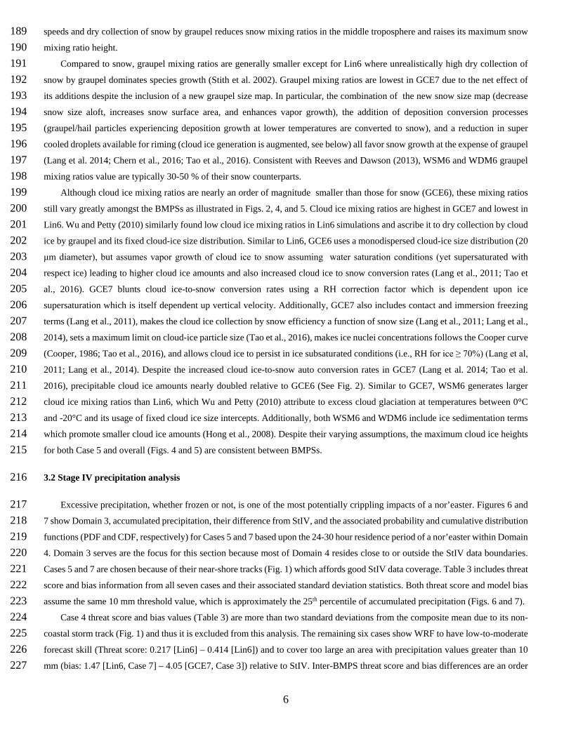
Compared to snow, graupel mixing ratios are generally smaller except for Lin6 where unrealistically high dry collection of 191 snow by graupel dominates species growth (Stith et al. 2002). Graupel mixing ratios are lowest in GCE7 due to the net effect of 192 its additions despite the inclusion of a new graupel size map. In particular, the combination of the new snow size map (decrease 193 snow size aloft, increases snow surface area, and enhances vapor growth), the addition of deposition conversion processes 194 (graupel/hail particles experiencing deposition growth at lower temperatures are converted to snow), and a reduction in super 195 cooled droplets available for riming (cloud ice generation is augmented, see below) all favor snow growth at the expense of graupel 196 (Lang et al. 2014; Chern et al., 2016; Tao et al., 2016). Consistent with Reeves and Dawson (2013), WSM6 and WDM6 graupel 197 mixing ratios value are typically 30-50 % of their snow counterparts. 198

Although cloud ice mixing ratios are nearly an order of magnitude smaller than those for snow (GCE6), these mixing ratios 199 still vary greatly amongst the BMPSs as illustrated in Figs. 2, 4, and 5. Cloud ice mixing ratios are highest in GCE7 and lowest in 200 Lin6. Wu and Petty (2010) similarly found low cloud ice mixing ratios in Lin6 simulations and ascribe it to dry collection by cloud 201 ice by graupel and its fixed cloud-ice size distribution. Similar to Lin6, GCE6 uses a monodispersed cloud-ice size distribution (20 202 μm diameter), but assumes vapor growth of cloud ice to snow assuming water saturation conditions (yet supersaturated with 203 respect ice) leading to higher cloud ice amounts and also increased cloud ice to snow conversion rates (Lang et al., 2011; Tao et 204 al., 2016). GCE7 blunts cloud ice-to-snow conversion rates using a RH correction factor which is dependent upon ice 205 supersaturation which is itself dependent up vertical velocity. Additionally, GCE7 also includes contact and immersion freezing 206 terms (Lang et al., 2011), makes the cloud ice collection by snow efficiency a function of snow size (Lang et al., 2011; Lang et al., 207 2014), sets a maximum limit on cloud-ice particle size (Tao et al., 2016), makes ice nuclei concentrations follows the Cooper curve 208 (Cooper, 1986; Tao et al., 2016), and allows cloud ice to persist in ice subsaturated conditions (i.e., RH for ice ≥ 70%) (Lang et al, 209 2011; Lang et al., 2014). Despite the increased cloud ice-to-snow auto conversion rates in GCE7 (Lang et al. 2014; Tao et al. 210 2016), precipitable cloud ice amounts nearly doubled relative to GCE6 (See Fig. 2). Similar to GCE7, WSM6 generates larger 211 cloud ice mixing ratios than Lin6, which Wu and Petty (2010) attribute to excess cloud glaciation at temperatures between 0°C 212 and -20°C and its usage of fixed cloud ice size intercepts. Additionally, both WSM6 and WDM6 include ice sedimentation terms 213 which promote smaller cloud ice amounts (Hong et al., 2008). Despite their varying assumptions, the maximum cloud ice heights 214 for both Case 5 and overall (Figs. 4 and 5) are consistent between BMPSs. 215

3.2 Stage IV precipitation analysis 216

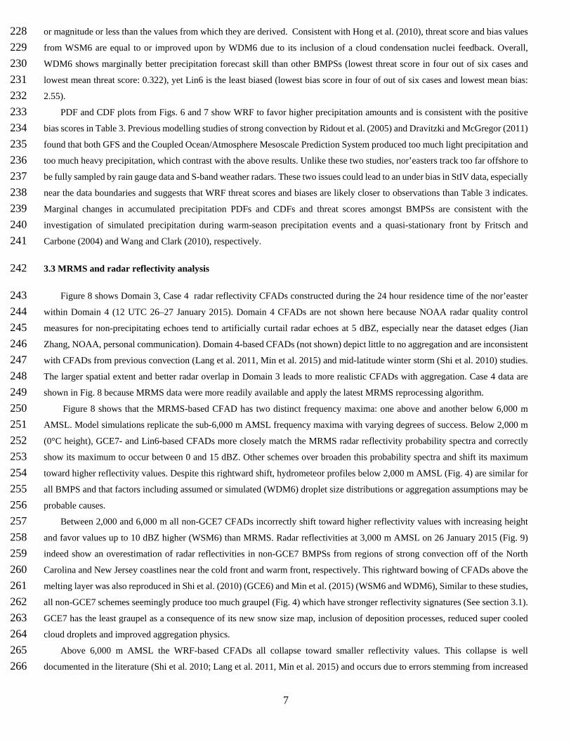
Excessive precipitation, whether frozen or not, is one of the most potentially crippling impacts of a nor’easter. Figures 6 and 217 7 show Domain 3, accumulated precipitation, their difference from StIV, and the associated probability and cumulative distribution 218 functions (PDF and CDF, respectively) for Cases 5 and 7 based upon the 24-30 hour residence period of a nor’easter within Domain 219 4. Domain 3 serves are the focus for this section because most of Domain 4 resides close to or outside the StIV data boundaries. 220 Cases 5 and 7 are chosen because of their near-shore tracks (Fig. 1) which affords good StIV data coverage. Table 3 includes threat 221 score and bias information from all seven cases and their associated standard deviation statistics. Both threat score and model bias 222 assume the same 10 mm threshold value, which is approximately the 25th percentile of accumulated precipitation (Figs. 6 and 7). 223

Case 4 threat score and bias values (Table 3) are more than two standard deviations from the composite mean due to its non-224 coastal storm track (Fig. 1) and thus it is excluded from this analysis. The remaining six cases show WRF to have low-to-moderate 225 forecast skill (Threat score: 0.217 [Lin6] – 0.414 [Lin6]) and to cover too large an area with precipitation values greater than 10 226 mm (bias: 1.47 [Lin6, Case 7] – 4.05 [GCE7, Case 3]) relative to StIV. Inter-BMPS threat score and bias differences are an order 227

7

or magnitude or less than the values from which they are derived. Consistent with Hong et al. (2010), threat score and bias values 228 from WSM6 are equal to or improved upon by WDM6 due to its inclusion of a cloud condensation nuclei feedback. Overall, 229 WDM6 shows marginally better precipitation forecast skill than other BMPSs (lowest threat score in four out of six cases and 230 lowest mean threat score: 0.322), yet Lin6 is the least biased (lowest bias score in four of out of six cases and lowest mean bias: 231 2.55). 232

PDF and CDF plots from Figs. 6 and 7 show WRF to favor higher precipitation amounts and is consistent with the positive 233 bias scores in Table 3. Previous modelling studies of strong convection by Ridout et al. (2005) and Dravitzki and McGregor (2011) 234 found that both GFS and the Coupled Ocean/Atmosphere Mesoscale Prediction System produced too much light precipitation and 235 too much heavy precipitation, which contrast with the above results. Unlike these two studies, nor’easters track too far offshore to 236 be fully sampled by rain gauge data and S-band weather radars. These two issues could lead to an under bias in StIV data, especially 237 near the data boundaries and suggests that WRF threat scores and biases are likely closer to observations than Table 3 indicates. 238 Marginal changes in accumulated precipitation PDFs and CDFs and threat scores amongst BMPSs are consistent with the 239 investigation of simulated precipitation during warm-season precipitation events and a quasi-stationary front by Fritsch and 240 Carbone (2004) and Wang and Clark (2010), respectively. 241

3.3 MRMS and radar reflectivity analysis 242

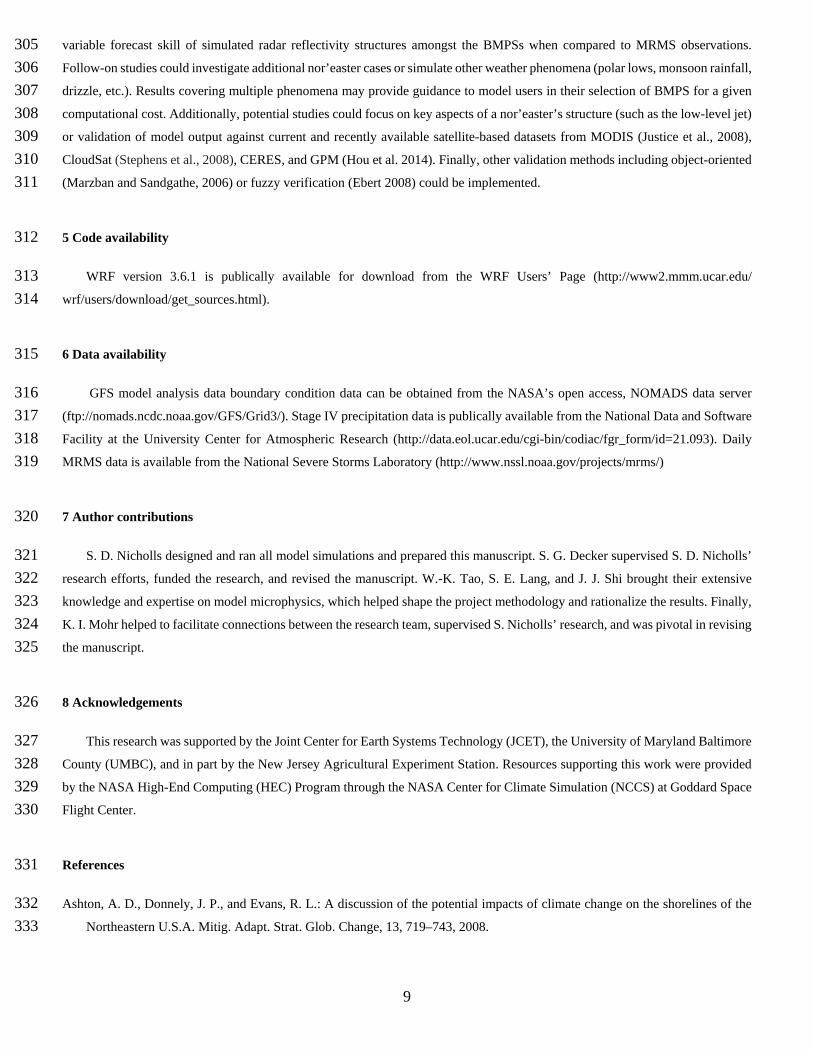
Figure 8 shows Domain 3, Case 4 radar reflectivity CFADs constructed during the 24 hour residence time of the nor’easter 243 within Domain 4 (12 UTC 26–27 January 2015). Domain 4 CFADs are not shown here because NOAA radar quality control 244 measures for non-precipitating echoes tend to artificially curtail radar echoes at 5 dBZ, especially near the dataset edges (Jian 245 Zhang, NOAA, personal communication). Domain 4-based CFADs (not shown) depict little to no aggregation and are inconsistent 246 with CFADs from previous convection (Lang et al. 2011, Min et al. 2015) and mid-latitude winter storm (Shi et al. 2010) studies. 247 The larger spatial extent and better radar overlap in Domain 3 leads to more realistic CFADs with aggregation. Case 4 data are 248 shown in Fig. 8 because MRMS data were more readily available and apply the latest MRMS reprocessing algorithm. 249

Figure 8 shows that the MRMS-based CFAD has two distinct frequency maxima: one above and another below 6,000 m 250 AMSL. Model simulations replicate the sub-6,000 m AMSL frequency maxima with varying degrees of success. Below 2,000 m 251 (0°C height), GCE7- and Lin6-based CFADs more closely match the MRMS radar reflectivity probability spectra and correctly 252 show its maximum to occur between 0 and 15 dBZ. Other schemes over broaden this probability spectra and shift its maximum 253 toward higher reflectivity values. Despite this rightward shift, hydrometeor profiles below 2,000 m AMSL (Fig. 4) are similar for 254 all BMPS and that factors including assumed or simulated (WDM6) droplet size distributions or aggregation assumptions may be 255 probable causes. 256

Between 2,000 and 6,000 m all non-GCE7 CFADs incorrectly shift toward higher reflectivity values with increasing height 257 and favor values up to 10 dBZ higher (WSM6) than MRMS. Radar reflectivities at 3,000 m AMSL on 26 January 2015 (Fig. 9) 258 indeed show an overestimation of radar reflectivities in non-GCE7 BMPSs from regions of strong convection off of the North 259 Carolina and New Jersey coastlines near the cold front and warm front, respectively. This rightward bowing of CFADs above the 260 melting layer was also reproduced in Shi et al. (2010) (GCE6) and Min et al. (2015) (WSM6 and WDM6), Similar to these studies, 261 all non-GCE7 schemes seemingly produce too much graupel (Fig. 4) which have stronger reflectivity signatures (See section 3.1). 262 GCE7 has the least graupel as a consequence of its new snow size map, inclusion of deposition processes, reduced super cooled 263 cloud droplets and improved aggregation physics. 264

Above 6,000 m AMSL the WRF-based CFADs all collapse toward smaller reflectivity values. This collapse is well 265 documented in the literature (Shi et al. 2010; Lang et al. 2011, Min et al. 2015) and occurs due to errors stemming from increased 266

8

entrainment of ambient air near cloud top and underlying aggregation assumptions made by each BMPS. Although each scheme 267 fully collapses by 7,500 m AMSL, the Goddard-based CFADs indicate a considerably steeper tilt in the maximum frequency core 268 as compared to other schemes, which is a likely byproduct of its higher snowfall mixing ratios (Fig. 4). Once above, 8,000 m 269 AMSL, MRMS radar reflectivity values show a second frequency maxima above 15 dBZ which is not replicated by WRF. Radar 270 reflectivities at 9,000 m AMSL on 26 January 2015 (Fig. 10) show precipitating echoes to occur offshore where the non-271 precipitating echo filtering applied in MRMS removed weak reflectivities and artificially shifting the CFAD toward higher values. 272

Finally, CFAD scores (Eq 2) with height and time (Fig. 11) provides a means to evaluate hourly forecast skill at each higher 273 level relative to MRMS. Figure 11 shows Lin6 and GCE7 to have notably improved forecast skill, especially between 2,000 and 274 4,850 m AMSL where increased graupel mixing ratios and droplet sizes which produced radar reflectivities higher than those from 275 MRMS. Despite their similar CFAD scores, CFAD structures (Fig. 8) and 3,000 m AMSL radar reflectivities (Fig. 9) do suggest 276 that GCE7 produces more realistic results than Lin6 where the rate of dry collection of snow by graupel is unrealistically high. In 277 short, Lin6 produces the right answer for the wrong reason, whereas GCE7 produces the correct answer with a more realistic 278 solution. Between 6,300 and 7,000 and m AMSL, GCE7 CFAD scores fall below all other schemes as a consequence of overly 279 small droplets from its aggregation simulations and cloud entrainment which cut off cloud tops at lower heights. The other six 280 cases produce similar tendencies in their CFAD and CFAD scores as noted above for Case 4, except cloud heights become higher 281 and CFADs become wider with the introduction of stronger convection in early and late season events. 282

4 Conclusions 283

The role and impact of five bulk microphysics schemes (BMPSs; Table 2) upon seven, Weather Research and Forecasting 284 model (WRF) winter time cyclone (“nor’easter”) simulations (Table 1) are investigated and validated against GFS model analysis 285 (GMA), Stage IV rain gauge and radar estimated precipitation, and the radar-derived, Multi-Radar, Multi-Sensor (MRMS) 3D 286 volume radar reflectivity product. Tested BMPSs include three single-moment, six class BMPSs (Lin6, GCE6, and WSM6), one 287 single-moment, seven class BMPS (GCE7), and one double-moment, six-class BMPS (WDM6). Simulated hydrometer mixing 288 ratios show general similarities for non-frozen hydrometeor species (cloud water and rain) due to their common Lin BMPS heritage. 289 However, frozen hydrometeor species (snow, graupel, cloud ice) demonstrate considerably larger variability amongst BMPSs. This 290 variability results from different assumptions concerning snow and graupel intercepts, degree of allowable ice supersaturation, 291 snow and graupel density maps, and terminal velocities made by each BMPS. WRF-simulated precipitation fields exhibit similar 292 coverage, but tend to favor higher precipitation amounts relative to Stage IV observations resulting in low-to-moderate threat 293 scores (0.217–0.414). Inter-model differences are an order of magnitude or less than the threat score values, but WDM6 does 294 demonstrate marginally better overall forecast skill. Finally, MRMS-based contoured frequency with altitude diagrams (CFADs) 295 and CFAD scores show Lin6 and GCE7 are best in the lower half of the troposphere, where GCE7 most realistically reproduced 296 the maximum frequency core between 5 and 15 dBZ due to its temperature and mixing ratio dependent aggregation and new snow 297 map. However, the overly large growth of graupel by dry collection of snow by graupel does suggest that Lin6 obtains high CFAD 298 scores with a less realistic solution than GCE7. Above 6,300 m AMSL, model simulations approach or exceed their cloud tops 299 where entrainment and hydrometeor sizes differences alter cloud top heights and reflectivity fields and non-precipitating echo 300 filtering in MRMS data make evaluations less meaningful with increasing height above cloud top. 301

This study has shown that although BMPS choice has minimal impact to the large-scale simulated environment, its effect upon 302 microphysical and precipitation properties of a nor’easter is more profound. No single BMPS demonstrated consistently improved 303 precipitation forecast skill as compared to other schemes, yet differences in their underlying microphysical assumptions does yield 304

9

variable forecast skill of simulated radar reflectivity structures amongst the BMPSs when compared to MRMS observations. 305 Follow-on studies could investigate additional nor’easter cases or simulate other weather phenomena (polar lows, monsoon rainfall, 306 drizzle, etc.). Results covering multiple phenomena may provide guidance to model users in their selection of BMPS for a given 307 computational cost. Additionally, potential studies could focus on key aspects of a nor’easter’s structure (such as the low-level jet) 308 or validation of model output against current and recently available satellite-based datasets from MODIS (Justice et al., 2008), 309 CloudSat (Stephens et al., 2008), CERES, and GPM (Hou et al. 2014). Finally, other validation methods including object-oriented 310 (Marzban and Sandgathe, 2006) or fuzzy verification (Ebert 2008) could be implemented. 311

5 Code availability 312

WRF version 3.6.1 is publically available for download from the WRF Users’ Page (http://www2.mmm.ucar.edu/ 313 wrf/users/download/get_sources.html). 314

6 Data availability 315

GFS model analysis data boundary condition data can be obtained from the NASA’s open access, NOMADS data server 316 (ftp://nomads.ncdc.noaa.gov/GFS/Grid3/). Stage IV precipitation data is publically available from the National Data and Software 317 Facility at the University Center for Atmospheric Research (http://data.eol.ucar.edu/cgi-bin/codiac/fgr_form/id=21.093). Daily 318 MRMS data is available from the National Severe Storms Laboratory (http://www.nssl.noaa.gov/projects/mrms/) 319

7 Author contributions 320

S. D. Nicholls designed and ran all model simulations and prepared this manuscript. S. G. Decker supervised S. D. Nicholls’ 321 research efforts, funded the research, and revised the manuscript. W.-K. Tao, S. E. Lang, and J. J. Shi brought their extensive 322 knowledge and expertise on model microphysics, which helped shape the project methodology and rationalize the results. Finally, 323 K. I. Mohr helped to facilitate connections between the research team, supervised S. Nicholls’ research, and was pivotal in revising 324 the manuscript. 325

8 Acknowledgements 326

This research was supported by the Joint Center for Earth Systems Technology (JCET), the University of Maryland Baltimore 327 County (UMBC), and in part by the New Jersey Agricultural Experiment Station. Resources supporting this work were provided 328 by the NASA High-End Computing (HEC) Program through the NASA Center for Climate Simulation (NCCS) at Goddard Space 329 Flight Center. 330

References 331

Ashton, A. D., Donnely, J. P., and Evans, R. L.: A discussion of the potential impacts of climate change on the shorelines of the 332 Northeastern U.S.A. Mitig. Adapt. Strat. Glob. Change, 13, 719–743, 2008. 333

10

Bosart, L. F.: The Presidents' Day Snowstorm of 18–19 February 1979: A subsynoptic-scale event, Mon. Wea. Rev., 109, 1542–334 1566, 1981. 335

Chen, F., and Dudhia, J.: Coupling an advanced land-surface/ hydrology model with the Penn State/ NCAR MM5 modeling system. 336 Part I: Model description and implementation, Mon. Wea. Rev., 129, 569–585, 2001. 337

Chern, J.-D., Tao, W.-K., Lang, S. E., Matsui, T., Li, J.-L. F., Mohr, K. I., Skofronick-Jackson, G. M., and Peters-Lidard, C. D.: 338 Performance of the Goddard multiscale modeling framework with Goddard ice microphysical schemes, J. Adv. Model. 339 Earth Syst., 7, doi:10.1002/2015MS000469, 2016. 340

Chou, M.-D. and Suarez, M. J.: A solar radiation parameterization for atmospheric research studies. NASA Tech, Memo 341 NASA/TM-1999-104606, 40 pp., 1999. 342

Chou, M.-D., and Suarez, M. J.: A thermal infrared radiation parameterization for atmospheric studies, NASA Tech. Rep. 343 NASA/TM-1999-10466, vol. 19, 55 pp., 2001. 344

Deng, M., Mace, G. G., Wang, Z., and Lawson, R. P.: Evaluation of several A-Train ice cloud retrieval products with in situ 345 measurements collected during the SPARTICUS campaign, J. Appl. Meteor. Climatol., 52, 1014–1030, 2013. 346

Dravitzki, S., and McGregor, J.: Predictability of heavy precipitation in the Waikato River Basin of New Zealand, Mon. Wea. 347 Rev., 139, 2184–2197, 2011. 348

Dudhia, J., Hong, S.-Y., and Lim, K.-S.: A new method for representing mixed-phase particle fall speeds in bulk microphysics 349 parameterizations, J. Meteor. Soc. Japan, 86A, 33–44, 2008. 350

Ebert, E. E.: Fuzzy verification of high-resolution gridded forecasts: A review and a proposed framework, Meteor. Applic., 15, 51-351 64, 2008. 352

Forbes, G. S., Thomson, D. W., and Anthes, R. A.: Synoptic and mesoscale aspects of an Appalachian ice storm associated with 353 cold-air damming, Mon. Wea. Rev., 115, 564–591, 1987. 354

Fulton, R. A., Breidenbach, J. P., Seo, D.-J., Miller, D. A., and O’Bannon, T.: The WSR-88D rainfall algorithm. Wea. 355 Forecasting, 13, 377–395. 1998. 356

Fritsch, J. M., and Carbone, R. E.: Improving quantitative precipitation forecasts in the warm season: A USWRP research and 357 development strategy, Bull. Amer. Meteor. Soc., 85, 955–965, 2004. 358

Ganetis, S. A. and Colle, B. A.: The thermodynamic and microphysical evolution of an intense snowband during the Northeast 359 U.S. blizzard of 8–9 February 2013. Mon. Wea. Rev., 143, 4104-4125, 2015. 360

Hong, S -Y., and Lim, J.-O. J.: The WRF single-moment 6-class microphysics scheme (WSM6), J. Korean Meteor. Soc., 42, 129-361 151, 2006. 362

Hong, S.-Y., Lim, K.-S. S., Lee, Y.-H., Ha, J.-C., Kim, H.-W., Ham, S.-J., and Dudhia, J.: Evaluation of the WRF double-363 moment 6-class microphysics scheme for precipitating convection, Adv. Meteor., 2010, doi:10.1155/2010/707253, 2010. 364

Hou, A. Y., Kakar, R. K., Neeck, S., Azarbarzin, A. A., Kummerow, C. D., Kojima, M., Oki, R., Nakamura, K., and Iguchi, T.: 365 The Global Precipitation Measurement Mission, Bull. Amer. Meteor. Soc., 95, 701–722, 2014. 366

Jacobs, N. A., Lackmann, G. M., and Raman, S.: The combined effects of Gulf Stream-induced baroclinicity and upper-level 367 vorticity on U.S. East Coast extratropical cyclogenesis, Mon. Wea. Rev., 133, 2494–2501, 2005. 368

Janjic, Z. I.: Nonsingular implementation of the Mellor–Yamada level 2.5 scheme in the NCEP meso model, NCEP Office Note 369 437, 61 pp., 2002. 370

Justice, C. O., Vermote, E., Townshend, J. R. G., Defries, R., et al.: The Moderate Resolution Imaging Spectroradiometer 371 (MODIS): land remote sensing for global change research, IEEE Transactions on Geoscience and Remote Sensing, 36, 372 1228–1249, 1998. 373

11

Kain, J. S.: The Kain–Fritsch Convective Parameterization: An Update, J. Appl. Meteor., 43, 170–181, 2004. 374 Kessler, E.: On the distribution and continuity of water substance in atmospheric circulation, Meteor. Monogr., 32, Amer. Meteor. 375

Soc., 84 pp, 1969. 376 Kleczek, M. A., Steenveld, G.-J., and Holtslag, A. A. M.: Evaluation of the Weather Research and Forecasting Mesoscale 377

Model for GABLS3: Impact of boundary-layer schemes, boundary conditions and spin-up, Boundary-Layer Meteorol, 152, 378 213–243, 2014. 379

Kocin, P. J. and Uccellini, L. W.: Northeast snowstorms. Vols. 1 and 2, Meteor. Monogr., No. 54., Amer. Met. Soc., 818 pp., 2004. 380 Kuo, Y. H., Low-Nam, S., and Reed, R. J.: Effects of surface energy fluxes during the early development and rapid intensification 381

stages of seven explosive cyclones in the Western Atlantic. Mon. Wea. Rev., 119, 457–476, 1991. 382 Lang, S., Tao, W.-K., Cifelli, R., Olson, W., Halverson, J., Rutledge, S., and Simpson, J.: Improving simulations of convective 383

system from TRMM LBA: Easterly and westerly regimes, J. Atmos. Sci., 64, 1141–1164, 2007. 384 Lang, S. E., Tao, W.-K., Zeng, X., and Li, Y.: Reducing the biases in simulated radar reflectivities from a bulk microphysics 385

scheme: Tropical convective systems, J. Atmos. Sci., 68, 2306–2320, 2011. 386 Lang, S. E., Tao, W.-K., Chern, J.-D., Wu, D., and Li, X.: Benefits of a fourth ice class in the simulated radar reflectivities of 387

convective systems using a bulk microphysics scheme, J. Atmos. Sci., 71, 3583–3612, doi:10.1175/JAS-D-13-0330.1, 2014. 388 Lebsock, M., and Su, H: Application of active spaceborne remote sensing for understanding biases between passive cloud water 389

path retrievals, J. Geophys. Res. Atmos., 119, 8962–8979, doi:10.1002/2014JD021568, 2014. 390 Li, J.-L. F., Waliser, D., Woods, C., Teixeira, J., Bacmeister, J., Chern, J.-D., Shen, B.-W., Tompkins, A., Tao, W.-K., and 391

Kohler, M.: Comparisons of satellites liquid water estimates to ECMWF and GMAO analyses, 20th century IPCC AR4 392 climate simulations, and GCM simulations, Geophys. Res. Lett., 35, L19710, doi:10.1029/2008GL035427, 2008. 393

Lim, K.-S. and Hong, S.-Y.: Development of an effective double-moment cloud microphysics scheme with prognostic cloud 394 condensation nuclei (CCN) for weather and climate models, Mon. Wea. Rev., 138, 1587–1612, 2010. 395

Lin, Y.-L., Farley, R. D., and Orville, H. D.: Bulk parameterization of the snow field in a cloud model, J. Climate Appl. Meteor., 396 22, 1065–1092, 1983. 397

Mailhot, J. and Chouinard, C.: Numerical forecasts of explosive winter storms: Sensitivity experiments with a meso-scale model, 398 Mon Wea. Rev., 117, 1311–1343, 1989. 399

Marzban, C., and Sandgathe, S.: Cluster analysis for verification of precipitation fields, Wea. Forecasting, 21, 824–838, 2006. 400 Mellor, G. L., and Yamada, T.: Development of a turbulence closure model for geophysical fluid problems, Rev. Geophys. Space 401

Phys., 20, 851–875, 1982. 402 Min, K.-H., S. Choo, D. Lee, and G. Lee: Evaluation of WRF cloud microphysics schemes using radar observations. Weather and 403

Forecasting, 30, 1571–1589, 2015. 404 Monin, A. S., and Obukhov, A. M.: Basic laws of turbulent mixing in the surface layer of the atmosphere. Tr. Akad. Nauk SSSR 405

Geophiz. Inst., 24, 163–187, 1954. 406 Morath, E.: Will a blizzard freeze U.S. economic growth for the third straight year, Wall Street Journal, 20 Jan. 2016. 407 Morrison, H., Thompson, G., and Tatarskii, V.: Impact of cloud microphysics on the development of trailing stratiform 408

precipitation in a simulated squall line: Comparison of one- and two-moment schemes, Mon. Wea. Rev., 137, 991–1007, 2009. 409 Mote, T. L., Gamble, D. W., Underwood, S. J., and Bentley, M. L.: Synoptic-scale features common to heavy snowstorms in the 410

Southeast United States, Wea. Forecasting, 12, 5–23, 1997. 411 Nicholls, S. D. and Decker, S. G.: Impact of coupling an ocean model to WRF nor’easter simulations, Mon. Wea. Rev., 143, 4997–412

5016, 2015. 413

12

Reeves, H. D. and Dawson II, D. T.: The dependence of QPF on the choice of microphysical parameterization for lake-effect 414 snowstorms, J. Appl. Meteor. Climatol., 52, 363–377, 2013. 415

Reisner, J. R., Rasmussen, R. M., and Bruintjes, R .T.: Explicit forecasting of super cooled liquid water in winter storms using the 416 MM5 mesoscale model. Quar. J. Roy. Met. Soc., 124, 1071–1107, 1998. 417

Ridout, J. A., Y. Jin, and Liou, C.-S.: A cloud-base quasi-balance constraint for parameterized convection: Application to the 418 Kain–Fritsch cumulus scheme, Mon. Wea. Rev., 133, 3315–3334, 2005. 419

Rutledge, S. A., and Hobbs, P. V.: The mesoscale and microscale structure and organization of clouds and precipitation in mid-420 latitude cyclones. XII: A diagnostic modeling study of precipitation development in narrow cloud-frontal rainbands. J. Atmos. 421 Sci., 20, 2949–2972, 1984. 422

Shi, J. J. et al.: WRF simulations of the 20-22 January 2007 snow events of Eastern Canada: Comparison with in situ and satellite 423 observations, J. Appl. Meteor. Climatol., 49, 2246–2266, 2010. 424

Skamarock, W.C., Klemp, J. P., Dudhia, J., Gill, D. O., Barker, D. M., Duda, M. G., Huang, X.-Y., Wang, W., and Powers, J. G.: 425 A description of the advanced research WRF version 3, NCAR Tech. Note NCAR/TN–475+STR, 125 pp., 2008. 426

Smith, A. B., and Katz, R. W.: US billion-dollar weather and climate disasters: Data sources, trends, accuracy and biases, 427 Natural Hazards, 67, 387–410, 2013. 428

Stark, D.: Field observations and modeling of the microphysics within winter storms over Long Island, NY. M.S. thesis, School 429 of Marine and Atmospheric Sciences, Stony Brook University, 132 pp., 2012. 430

Stauffer, D. R., and Warner, T. T.: A numerical study of Appalachian cold-air damming and coastal frontogenesis, Mon. Wea. 431 Rev., 115, 799–821, 1987. 432

Stephens, G. L., et al.: CloudSat mission: Performance and early science after the first year of operation, J. Geophys. Res., 113, 433 D00A18, doi:10.1029/2008JD009982, 2008. 434

Stith, J. L., Dye, J. E., Bansemer, A., Heymsfield, A. J., Grainger, C. A., Petersen, W. A, and Clfelli, R.: Microphysical 435 observations of tropical clouds, J. Appl. Meteor., 41, 97–117, 2002. 436

Tao, W.-K., Simpson, J. and McCumber, M.: An ice-water saturation adjustment, Mon. Wea. Rev., 117, 231–235, 1989. 437 Tao, W.-K., Shi, J. J., Chen, S. S., Lang, S., Lin, P.-L., Hong, S.-Y., Peters-Lidard, C., and Hou, A.: The impact of microphysical 438

schemes on hurricane intensity and track, Asia-Pacific J. Atmos. Sci., 47, 1–16, 2011. 439 Tao, W.-K., Wu, D., Lang, S., Chern, J.-D., Peters-Lidard, C., Fridlind, A., and Matsui, T.: High-resolution NU-WRF simulations 440

of a deep convective-precipitation system during MC3E: Further improvements and comparisons between Goddard 441 microphysics schemes and observations, J. Geophys. Res. Atmos., 121, 1278–1305, doi:10.1002/2015JD023986, 2016. 442

Uccellini, L. W. and Kocin, P. J.: The Interaction of jet streak circulations during heavy snow events along the east coast of the 443 United States, Wea. Forecasting, 2, 289–308, 1987. 444

Wang, S.-Y., and Clark, A. J.: NAM Model forecasts of warm-season quasi-stationary frontal environments in the Central United 445 States, Wea. Forecasting, 25, 1281–1292, 2010. 446

Wilks, D. S.: Statistical methods in the atmospheric sciences, third edition, Academic Press, Oxford, in press., 2011. 447 Wu, L., and Petty, G. W.: Intercomparison of bulk microphysics schemes in model simulations of polar lows, Mon. Wea. Rev., 448

138, 2211–2228, 2010. 449 Yao, Y., Pierre, W., Zhang, W., and Jiang, J.: Characteristics of atmosphere-ocean interactions along North Atlantic extratropical 450

storm tracks, J. Geophys. Res., 113, doi:10.1029/2007JD008854, 2008. 451 Yuter, S. E., and Houze, R. A.: Three-dimensional kinematic and microphysical evolution of Florida cumulonimbus part II: 452

frequency distributions of vertical velocity, reflectivity, and differential reflectivity, Mon. Wea. Rev., 123, 1941–1963. 453

13

Zhang, J., Howard, K., Langston, C., Vasiloff, S., Kaney, B., Arthur, A., et al.: National mosaic and multi-sensor QPE (NMQ) 454 system: description, results, and future plans. Bulletin of the American Meteorological Society, 92, 1321-1338, 2011. 455

Zhang, J., Howard, K., Langston, C., Kaney, B., Qi, Y., Tang, L., Grams, H., Wang, Y., Cocks, S., Martinaitis, S., and Arthur, A.: 456 Multi-radar multi-sensor (MRMS) quantitative precipitation estimation: Initial operating capabilities. Bull. Amer. Meteor. 457 Soc., 97, 621–638, 2016. 458

14

Table 1. Nor’easter case list. The NESIS number is included for storm severity reference. Mean sea-level pressure (MSLP) indicates 459 maximum cyclone intensity in GMA. The last two columns denote the first and last times for each model run. GMA storm tracks are 460 displayed in Fig. 1. 461 462

Case

Number NESIS

MSLP

(hPa) Event Dates

Model Run Start

Date

Model Run End

Date

1 N/A 991.5 15–16 Oct 2009 10/15 00UTC 10/20 00UTC

2 N/A 989.5 07–09 Nov 2012 11/06 18UTC 11/11 18UTC

3 4.03 972.6 19–20 Dec 2009 12/18 18UTC 12/23 18UTC

4 2.62 980.5 26–28 Jan 2015 01/25 12UTC 01/30 12 UTC

5 4.38 979.7 05–07 Feb 2010 02/05 06UTC 02/10 06UTC

6 1.65 1005.5 02–03 Mar 2009 03/01 00UTC 03/06 00UTC

7 N/A 993.5 12–14 Mar 2010 03/11 18UTC 03/16 18UTC

463 464

15

Table 2. Applied bulk microphysics schemes and their characteristics. The below table indicates simulated mixing ratio species and 465 number of moments. Mixing ratio species include: QV = water vapor, QC = cloud water, QH = hail, QI = cloud ice, QG = graupel, QR 466 = rain, QS = snow. 467

Microphysics

Scheme QV QC QH QI QG QR QS Moments Citation

Lin6 X X X X X X 1 Lin et al. (1983);

Rutledge and Hobbs (1984)

GCE6 X X X X X X 1 Tao et al. (1989);

Lang et al. (2007)

GCE7 X X X X X X X 1 Lang et al. (2014)

WSM6 X X X X X X 1 Hong and Lim (2006)

WDM6 X X X X X X 2 (QC, QR) Lim and Hong (2010)

468

16

Table 3. Domain 3, Stage IV-relative, accumulated precipitation threat scores and biases assuming a threshold value of 10 mm (25th 469 percentile of 24 hour accumulated precipitation). Bolded value denote the model simulation with the threat score closest to 1 (perfect 470 forecast) or a bias values closest to 1 (number of forecasted cells matches observations). The lower two panels indicate the number of 471 standards deviations (stdev) each threat score and bias value deviates from the composite (all models + all cases) mean. 472

Threat Score 1 2 3 4 5 6 7 Mean Mean w/o 4

Lin6 0.289 0.217 0.291 0.091 0.414 0.304 0.332 0.277 0.308 GCE6 0.286 0.243 0.320 0.091 0.406 0.291 0.356 0.285 0.317 GCE7 0.288 0.235 0.319 0.096 0.405 0.300 0.337 0.283 0.314 WSM6 0.293 0.237 0.315 0.093 0.404 0.292 0.356 0.284 0.316 WDM6 0.290 0.243 0.329 0.094 0.411 0.299 0.357 0.289 0.322

Bias 1 2 3 4 5 6 7 Mean Mean w/o 4 Lin6 2.47 3.53 2.72 7.82 2.22 2.9 1.47 3.30 2.55

GCE6 2.37 3.88 2.85 8.09 2.26 2.93 1.64 3.43 2.65 GCE7 2.52 4.05 2.85 7.75 2.23 2.82 1.57 3.40 2.67 WSM6 2.47 3.75 2.86 8.13 2.26 2.93 1.62 3.43 2.64 WDM6 2.37 3.8 2.76 8.09 2.23 2.82 1.57 3.37 2.59

T. Score

Stats: All

Stdev 0.094 All Mean 0.284

Threat Score 1 2 3 4 5 6 7

Lin6 0.06 -0.71 0.08 -2.05 1.39 0.22 0.52

GCE6 0.03 -0.43 0.39 -2.05 1.31 0.08 0.77

GCE7 0.05 -0.52 0.38 -2.00 1.29 0.18 0.57

WSM6 0.10 -0.50 0.34 -2.03 1.28 0.09 0.77

WDM6 0.07 -0.43 0.48 -2.02 1.36 0.16 0.78

Bias Stats All Stdev 2.007 All

Mean 3.389

Bias 1 2 3 4 5 6 7

Lin6 -0.46 0.07 -0.33 2.21 -0.58 -0.24 -0.96

GCE6 -0.51 0.24 -0.27 2.34 -0.56 -0.23 -0.87

GCE7 -0.43 0.33 -0.27 2.17 -0.58 -0.28 -0.91

WSM6 -0.46 0.18 -0.26 2.36 -0.56 -0.23 -0.88

WDM6 -0.51 0.21 -0.31 2.34 -0.58 -0.28 -0.91

473

474

17

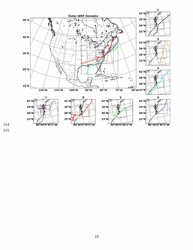
List of Figure Captions 475 476 Figure 1. Nested WRF configuration used in simulations. The large panel shows the first 3 model domains (45-, 15-, 5- km 477 grid spacing, respectively). The smaller panels show the location of domain 4 (1.667-km resolution) for each of the seven 478 cases. The colored lines show the cyclone track as indicated by GMA for each nor’easter case. 479

Figure 2. Domain 4 (1.667 km grid spacing), precipitable mixing ratios (mm) at 06 UTC 06 February 2010. Shown 480 abbreviations for mixing ratios include: QV = water vapor, QC = cloud water, QG = graupel, QI = cloud ice, QR = rain, 481 QS = snow. 482

Figure 3. Simulated radar reflectivity (dBZ) at 4,000 m above mean sea level and their difference at the same time as Fig. 483 2. 484

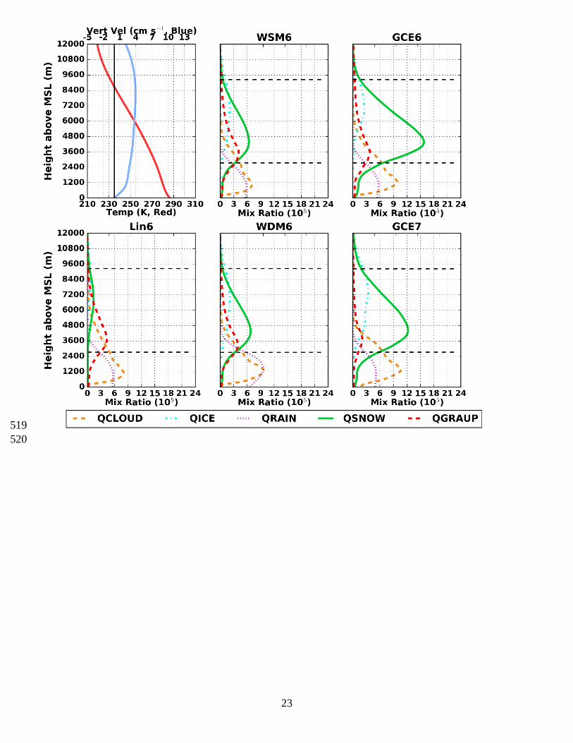
Figure 4. Domain 4-averaged (1.167-km grid spacing) mixing ratios (kg kg-1), temperature (K), and vertical velocity (cm s-1) 485 at the same time as Fig. 2. . The black dashed lines denote the height above mean sea level (MSL) where the air temperature 486 is 0°C or -40°C. The upper-left panel shows composited and model-averaged profiles of temperature (red line) and vertical 487 velocity (blue). Mixing ratio species abbreviations are QCLOUD (cloud water), QGRAUP (graupel), QICE (cloud ice), 488 QRAIN (rain), QSNOW (snow) and QHAIL (hail). 489

Figure 5. Domain 4-averaged (1.167-km grid spacing), composite mixing ratios (kg kg-1), temperature (K), and vertical 490 velocities (cm s-1) composited over all seven nor’easter events. The black dashed lines denote the height above mean sea level 491 (MSL) where the air temperature is 0°C or -40°C. The upper-left panel shows composited and model-averaged profiles of 492 temperature (red line) and vertical velocity (blue). Mixing ratio species abbreviations are QCLOUD (cloud water), QGRAUP 493 (graupel), QICE (cloud ice), QRAIN (rain), QSNOW (snow) and QHAIL (hail). 494

Figure 6. Case 5, 24-hour precipitation accumulation and their differences (mm, small panels) and corresponding 495 probability density and cumulative distribution functions (big panel) of these same data derived from Stage IV and WRF 496 model output. Accumulation period is from 00 UTC 06 February 2010 – 00 UTC 07 February 2010. Shown differences are 497 model - Stage IV (StIV). 498

Figure 7. Case 7, 24-hour precipitation accumulation and their differences (mm, small panels) and corresponding 499 probability density and cumulative distribution functions (big panel) of these same data derived from Stage IV and WRF 500 model output. Accumulation period is from 18 UTC 12 March 2010 – 18 UTC 13 March 2010. Shown differences are 501 model - Stage IV (StIV). 502

Figure 8. Domain 3 (5 km grid spacing), contoured frequency with altitude diagram (CFAD) of radar reflectivity and 503 indicated differences from Case 4 (January 2015). Data accumulation period spans 12 UTC 26 January 2015 – 12 UTC 27 504 January 2015 during the transit of the nor’easter through Domain 4. The y-axis shows height above mean sea level (HMSL). 505

Figure 9. MRMS radar reflectivity and WRF simulated radar reflectivity (dBZ) at 3,000 m above sea level at 18 UTC 26 506 January 2015. Show radar reflectivity differences are as indicated. 507

Figure 10. MRMS observed radar and WRF simulated radar reflectivity (dBZ) at 9,000 m above sea level at 18 UTC 26 508 January 2015. Show radar reflectivity differences are as indicated. 509

18

Figure 11. Domain 3, (5 km grid spacing), hourly CFAD scores (See Eq. 2) of radar reflectivity and indicated differences 510 from Case 4 starting 12 UTC 26 January 2015 and ending on 12 UTC 27 January 2015. The time period corresponds to 511 the same time period as in Figure 5. The y-axis shows height above mean sea level (m). 512

513

19

514 515

20

516

21

517

22

518

23

519 520

24

521

25

522

26

523

27

524

28

525

29

526