INFLUENCE OF COMPRESSION RATIO ON THE PERFORMANCE ...
185
INFLUENCE OF COMPRESSION RATIO ON THE PERFORMANCE CHARACTERISTICS OF A SPARK IGNITION ENGINE By AINA TOPE DEPARTMENT OF MECHANICAL ENGINEERING AHMADU BELLO UNIVERSITY, ZARIA NIGERIA FEBRUARY, 2012
Transcript of INFLUENCE OF COMPRESSION RATIO ON THE PERFORMANCE ...
INFLUENCE OF COMPRESSION RATIO ON THE PERFORMANCE
CHARACTERISTICS OF A SPARK IGNITION ENGINE
By
AINA TOPE
DEPARTMENT OF MECHANICAL ENGINEERING
AHMADU BELLO UNIVERSITY, ZARIA
NIGERIA
FEBRUARY, 2012
ii
INFLUENCE OF COMPRESSION RATIO ON THE PERFORMANCE
CHARACTERISTICS OF A SPARK IGNITION ENGINE
BY
AINA TOPE
MSC/ENG/11404/2007-08
A THESIS SUBMITTED TO THE POST GRADUATE SCHOOL, AHMADU
BELLO UNIVERSITY, ZARIA
IN PARTIAL FULFILMENT OF THE AWARD OF MASTERS OFSCIENCE IN MECHANICAL ENGINEERING (ENERGY)
MECHANICAL ENGINEERING DEPARMENT
FACULTY OF ENGINEERING
AHMADU BELLO UNIVERSITY
ZARIA
FEBRUARY, 2012
iii
DECLARATION
I declare that the work in this thesis titled ‘’INFLUENCE OF COMPRESSION RATIO
ON THE PERFORMANCE CHARACTERISTICS OF A SPARK IGNITION ENGINE’’
has been performed by me in the Department of Mechanical Engineeringunder the
supervision of Prof. C.O. Folayan and Dr. G.Y. Pam.
The information derived from the literature has been duly acknowledged in the text and a
list of references provided. No part of this work has been presented for another degree or
diploma at any university.
Aina, Tope
Name of student (Signature) (Date)
iv
CERTIFICATION
This thesis entitled ‘’INFLUENCE OF COMPRESSION RATIO ON THE PERFORMANCE
CHARACTERISTICS OF A SPARK IGNITION ENGINE’’ by Aina, Topemeets the
regulations governing the award of the degree of Master of Science ofAhmadu Bello
University, Zaria, and is approved for its contribution to knowledge and literary presentation.
Prof. C.O. Folayan Chairman, Supervisory Committee (Signature) (Date)
Dr. G.Y. Pam Member, Supervisory Committee (Signature) (Date)
Dr. D.S. Yawas Head of Department (Signature) (Date)
Prof. A. A. Joshua Dean, School of Postgraduate Studies (Signature) (Date)
v
ACKNOWLEDGEMENTS
I give glory and honour to Almighty God for His immeasurable help at every time of my
need. I thank God so much for seeing me through the course of this research.
I wish to express my profound gratitude to my able supervisors, Prof. C.O. Folayan and Dr.
G.Y. Pam both of the department of Mechanical Engineering, Ahmadu Bello University,
Zaria for their immense contributions and guidance in ensuring the successful completion of
this research.
Special thanks to all my lecturers in Mechanical Engineering Department especially the
head of department in the person of Dr. D.S. Yawas, Dr. F.O. Anafiand Dr. Mrs. R.B.O
Suleiman (for her encouragement and support with the Engineering Equation Solver (EES)
computer programme used in this research). Further, my sincere gratitude goes to all the
non-academic staff of the department especially AlhajiShehuModele for all the valuable
ideas and assistance in the departmental laboratory.
My appreciation goes to my brothers and sisters:Mr. AnthonyOluwasegunAina, Engr.
ToyinAinaand Mrs. Beatrice MopelolaAdedayo. I also appreciate the efforts of my
friends:Miss. ObiageliNnekaNze, Mr. Bakare Samuel and Kehinde Adebayo.
This section will lack completeness without mentioning my “parents”, Mrs. C.A. Akolo
and Mr. J. Joriah
vi
ABSTRACT
The need to improve the performance characteristics of the gasoline engine has necessitated
the present research. Increasing the compression ratio below detonating values to improve
on the performance is an option. The compression ratio is a factor that influences the
performance characteristics of internal combustion engines. This work is a an experimental
and theoretical investigation of the influence of the compression ratio on the brake power,
brake thermal efficiency, brake mean effective pressure and specific fuel consumption of
aRicardo variable compression ratio spark ignition engine. A range of compression ratios of
5, 6, 7, 8 and 9, and engine speeds of1100 to 1600rpm, in increments of 100rpm, were
utilised. The results showsthat as the compression ratio increases, the actual fuel
consumption decreasesaveragely by 7.75%, brake thermal efficiency improves by 8.49 %
and brake power also improves by 1.34%. The optimum compression ratio corresponding to
maximum brake power, brake thermal efficiency, brake mean effective pressure and lowest
specific fuel consumption is 9.The theoretical values were compared with experimental
values. The grand averages of the percentage errorsbetween the theoretical and experimental
valuesfor all the parameters were evaluated. The small values of the percentage errors
between the theoretical and experimental values show that there is agreement between the
theoretical and experimental performance characteristics of the engine.
vii
TABLE OF CONTENTS
TITLE PAGE
COVER PAGE . . . . . . . . i
TITLE PAGE . . . . . . . . . iii
DECLARATION . . . . . . . . iv
CERTIFICATION . . . . . . . . v
ACKNOWLEDGEMENTS . . . . . . . vi
ABSTRACT . . . . . . . . . vii
TABLE OF CONTENTS . . . . . . . viii
LIST OF FIGURES . . . . . . . . xiii
LIST OF TABLES . . . . . . . . xix
LIST OF PLATES . . . . . . . . xxiv
LIST OF APPENDICES . . . . . . . xxv
ABBREVIATIONS AND SYMBOLS . . . . . xxvi
viii
CHAPTER ONE: INTRODUCTION
1.1 Advantages and Applications of Internal Combustion (IC)
Engines . . . . . . . . 2
1.2 Thermal efficiency of IC engines . . . . . 3
1.3 Effect of Compression Ratio on the Thermal Efficiency of SI Engine 5
1.4 Statement of the problem . . . . . . 6
1.5 The Present Research . . . . . . . 7
1.6 Aim and Objectives . . . . . . 7
1.7 Significant of Research . . . . . . 8
CHAPTER TWO: LITERATURE REVIEW
2.1 Review of Related Past Works . . . . . 9
2.2 The Four Stroke Internal Combustion (IC) Engine . . 15
2.2.1 Structure and operation of a four stroke SI engine . . 15
2.3 Engine Performance Parameters . . . . 17
2.3.1 Definition of essential parameters . . . . 18
CHAPTER THREE: MATERIALS AND METHODS
3.1 Description of Test Engine . . . . . . 22

ix
3.2 Experimental Set-up of the Ricardo Variable Compression Ratio Engine. 22
3.3 The Engine . . . . . . . . 24
3.4 The Fuel System. . . . . . . . 25
3.5 Repairs of the Ricardo Engine . . . . . 25
3.5.1 Repairs of the central cooling system into the laboratory . 26
3.5.2 Repairs on the electric motor . . . . 26
3.5.3 Repairs of the fuel system . . . . 26
3.5.4 Repairs of the ignition system. . . . . 27
3.5.5 Replacement of the conveyor belt for the Tachometer . 27
3.6 Variation of the Compression Ratio . . . . . 27
3.7 Experimental Procedure . . . . . . 29
3.7.1 Calibration of the Ricardo engine . . . . 29
3.7.2 Test Procedure . . . . . . 30
3.8 Calculation of Mass Flow Rate of the Fuel . . . . 31
3.9 Measurement of Air Consumption . . . . . 32
3.10 Operation of the Ricardo Engine and Measurement of Break Load 33
3.11 Theoretical Determination of Performance Characteristics . . 34
x
3.11.1 Calculation of torque gain/loss . . . . 34
3.11.2 Error analysis . . . . . . 36
CHAPTER FOUR: RESULTS AND DISCUSSION
4.1 Discussion of Results . . . . . . 48
4.1.1 Effect of varying experimental compression ratio on the engine
brake power . . . . . . . 48
4.1.2 Effect of varying experimental compression ratio on the engine
brakethermal efficiency . . . . . 48
4.1.3 Effect of varying the experimental compression ratio on
brake mean effective pressure. . . . . 49
4.1.4 Effect of varying experimental compression ratio on the
fuel consumption parameters . . . . . 50
4.1.5 Effect of varying experimental compression ratio on
the volumetric efficiency . . . . . 50
4.2 Improvement in the Engine Performance Characteristics from
Increase in the Compression Ratio . . . . 51
xi
4.3 Comparison between the Experimental and Theoretical values . 53
4.4 Comparison between Experimental and Theoretical Performance . 80
4.4.1 Brake power . . . . . . . 80
4.4.2 Brake thermal efficiency . . . . . 81
4.4.3 Specific fuel consumption . . . . . 81
4.4.4 Brake mean effective pressure . . . . 82
CHAPTER FIVE: SUMMARY, CONCLUSIONS AND RECOMMENDATIONS
5.1 Summary . . . . . . . . 83
5.2 Conclusions . . . . . . . . 85
5.3 Recommendations . . . . . . . 86
REFERENCES . . . . . . . . 87
APPENDICES . . . . . . . . 90
xii
LIST OF FIGURES
Figure 1.1. Electric power generation by IC engine . . . 2
Figure 1.2. Engine classification chart. . . . . . 3
Figure 2.1. Schematic diagram of the Retrofit test engine. . . 11
Figure 2.2. Main components of an IC engine . . . . 15
Figure 2.3. The operations of an engine on four stroke cycle . . 16
Figure 3.1. Schematic diagram of the Ricardo variable compression ratio engine
. . . . . . . 23
Figure 3.2. Schematic diagram of the fuel system . . . 25
Figure 3.3. Schematic diagram showing the cylinder head, clearance volume and the
displaced volume in a spark ignition (SI) engine. . 28
Figure 4.1. Variation of experimental brake power with compression ratio
for different engine speeds . . . . . 43
Figure 4.2. Variation of experimental brake power with engine speed for different
compression ratios . . . . . 44
Figure 4.3. Variation of experimental thermal efficiency with compression ratio for
different engine speeds . . . . 44
Figure 4.4. Variation of experimental thermal efficiency with engine speed for
different compression ratios . . . 45
xiii
Figure 4.5. Variation of brake mean effective pressure with compression ratio
for different engine speeds . . . . . 45
Figure 4.6. Variation of brake mean effective pressure with engine speed fordifferent
compression ratios . . . . . 46
Figure 4.7. Variation of experimental specific fuel consumption with compression ratio
for different engine speeds . . 46
Figure 4.8. Variation of experimental specific fuel consumption with engine speed for
different compression ratios . . . 47
Figure 4.9. Variation of experimental volumetric efficiency with compression ratio for
different engine speeds . . . . 47
Figure 4.10. Variation of brake power with compression ratio at engine speed of
1100 rpm. . . . . . . . 58
Figure 4.11. Variation of brake power with compression ratio at engine speed of
1200 rpm. . . . . . . . 58
Figure 4.12. Variation of brake power with compression ratio at engine speed of
1300 rpm. . . . . . . . 59
Figure 4.13. Variation of brake power with compression ratio at engine speed of
1400 rpm. . . . . . . . 59
Figure 4.14. Variation of brake power with compression ratio at engine speed of
1500 rpm. . . . . . . . 60
xiv
Figure 4.15. Variation of brake power with compression ratio at engine speed of
1600 rpm. . . . . . . . 60
Figure 4.16. Variation of brake thermal efficiency with compression ratio at
engine speedof 1100 rpm . . . . . 61
Figure 4.17. Variation of brake thermal efficiency with compression ratio at
engine speed of 1200 rpm . . . . . 61
Figure 4.18. Variation of brake thermal efficiency with compression ratio at
engine speed of 1300 rpm . . . . . 62
Figure 4.19. Variation of brake thermal efficiency with compression ratio at engine
speed of 1400 rpm . . . . . . 62
Figure 4.20. Variation of brake thermal efficiency with compression ratio at
engine speed of 1500 rpm . . . . . 63
Figure 4.21. Variation of brake thermal efficiency with compression ratio at
engine speed of 1600 rpm . . . . . 63
Figure 4.22. Variation of specific fuel consumption with compression ratio at
engine speed of 1100 rpm . . . . . 64
Figure 4.23. Variation of specific fuel consumption with compression ratio at
enginespeed of 1200 rpm . . . . . 64
Figure 4.24. Variation of specific fuel consumption with compression ratio at enginespeed
of 1300 rpm . . . . . 65
xv
Figure 4.25. Variation of specific fuel consumption with compression ratio at
engine speed of 1400 rpm . . . . . 65
Figure 4.26. Variation of specific fuel consumption with compression ratio at
engine speed of 1500 rpm . . . . . 66
Figure 4.27. Variation of specific fuel consumption with compression ratio at
engine speed of 1600 rpm . . . . . 66
Figure 4.28. Variation of brake mean effective pressure with compression ratio at
engine speed of 1100 rpm . . . . . 67
Figure 4.29. Variation of brake mean effective pressure with compression ratio at
engine speed of 1200 rpm . . . . . 67
Figure 4.30. Variation of brake mean effective pressure with compression ratio at
engine speed of 1300 rpm . . . . . 68
Figure 4.31. Variation of brake mean effective pressure with compression ratio at
engine speed of 1400 rpm . . . . . 68
Figure 4.32. Variation of brake mean effective pressure with compression ratio at
engine speed of 1500 rpm . . . . . 69
Figure 4.33. Variation of brake mean effective pressure with compression ratio at
engine speed of 1600 rpm . . . . . 69
Figure 4.34. Variation of brake power with engine speed at compression ratio of 5
. . . . . . . . . 70
xvi
Figure 4.35. Variation of brake power with engine speed at compression ratio of 6
. . . . . . . . . 70
Figure 4.36. Variation of brake power with engine speed at compression ratio of 7
. . . . . . . . . 71
Figure 4.37. Variation of brake power with engine speed at compression ratio of 8
. . . . . . . . . 71
Figure 4.38. Variation of brake power with engine speed at compression ratio of 9
. . . . . . . . . 72
Figure 4.39. Variation of brake thermal efficiency with engine speed at compression
ratio of 5 . . . . . . . 72
Figure 4.40. Variation of brake thermal efficiency with engine speed at compression
ratio of 6 . . . . . . . 73
Figure 4.41. Variation of brake thermal efficiency with engine speed at compression
ratio of 7 . . . . . . . 73
Figure 4.42. Variation of brake thermal efficiency with engine speed at compression
ratio of 8 . . . . . . . 74
Figure 4.43. Variation of brake thermal efficiency with engine speed at compression
ratio of 9 . . . . . . . 74
Figure 4.44. Variation of specific fuel consumption with engine speed at compression
ratio of 5 . . . . . . . 75
xvii
Figure 4.45. Variation of specific fuel consumption with engine speed at compression
ratio of 6 . . . . . . . 75
Figure 4.46. Variation of specific fuel consumption with engine speed at compression
ratio of 7 . . . . . . . 76
Figure 4.47. Variation of specific fuel consumption with engine speed at compression
ratio of 8 . . . . . . . 76
Figure 4.48. Variation of specific fuel consumption with engine speed at compression
ratio of 9 . . . . . . 77
Figure 4.49. Variation of brake mean effective pressure with engine speed at
compression ratio of 5 . . . . . 77
Figure 4.50. Variation of brake mean effective pressure with engine speed at
compression ratio of 6 . . . . . 78
Figure 4.51. Variation of brake mean effective pressure with engine speed at
compression ratio of 7 . . . . . 78
Figure 4.52. Variation of brake mean effective pressure with engine speed at
compression ratio of 8 . . . . . 79
Figure 4.53. Variation of brake mean effective pressure with engine speed at
compression ratio of 9 . . . . . 79
xviii
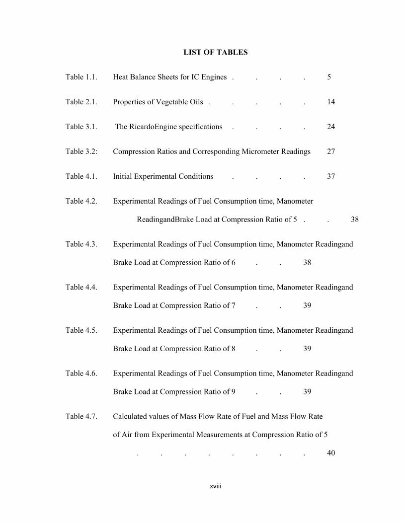
LIST OF TABLES
Table 1.1. Heat Balance Sheets for IC Engines . . . . 5
Table 2.1. Properties of Vegetable Oils . . . . . 14
Table 3.1. The RicardoEngine specifications . . . . 24
Table 3.2: Compression Ratios and Corresponding Micrometer Readings 27
Table 4.1. Initial Experimental Conditions . . . . 37
Table 4.2. Experimental Readings of Fuel Consumption time, Manometer
ReadingandBrake Load at Compression Ratio of 5 . . 38
Table 4.3. Experimental Readings of Fuel Consumption time, Manometer Readingand
Brake Load at Compression Ratio of 6 . . 38
Table 4.4. Experimental Readings of Fuel Consumption time, Manometer Readingand
Brake Load at Compression Ratio of 7 . . 39
Table 4.5. Experimental Readings of Fuel Consumption time, Manometer Readingand
Brake Load at Compression Ratio of 8 . . 39
Table 4.6. Experimental Readings of Fuel Consumption time, Manometer Readingand
Brake Load at Compression Ratio of 9 . . 39
Table 4.7. Calculated values of Mass Flow Rate of Fuel and Mass Flow Rate
of Air from Experimental Measurements at Compression Ratio of 5
. . . . . . . . 40
xix
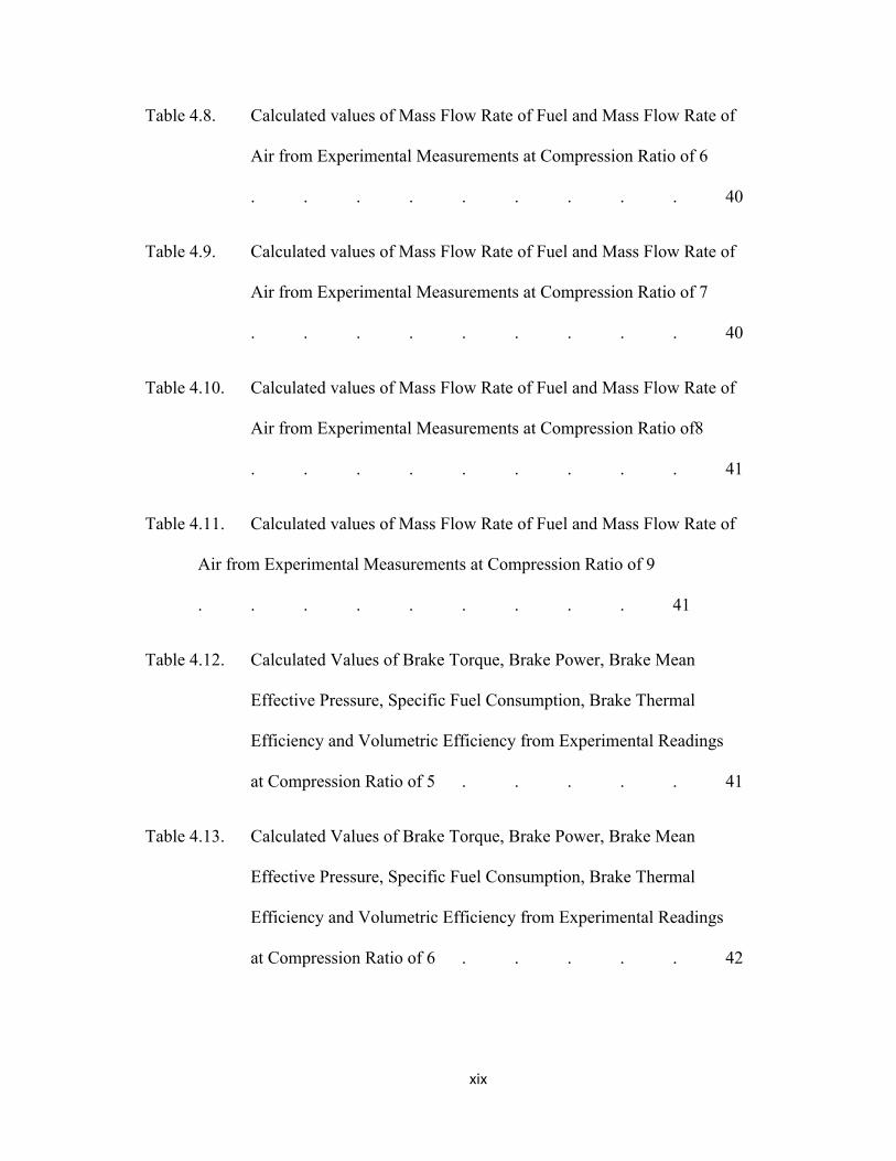
Table 4.8. Calculated values of Mass Flow Rate of Fuel and Mass Flow Rate of
Air from Experimental Measurements at Compression Ratio of 6
. . . . . . . . . 40
Table 4.9. Calculated values of Mass Flow Rate of Fuel and Mass Flow Rate of
Air from Experimental Measurements at Compression Ratio of 7
. . . . . . . . . 40
Table 4.10. Calculated values of Mass Flow Rate of Fuel and Mass Flow Rate of
Air from Experimental Measurements at Compression Ratio of8
. . . . . . . . . 41
Table 4.11. Calculated values of Mass Flow Rate of Fuel and Mass Flow Rate of
Air from Experimental Measurements at Compression Ratio of 9
. . . . . . . . . 41
Table 4.12. Calculated Values of Brake Torque, Brake Power, Brake Mean
Effective Pressure, Specific Fuel Consumption, Brake Thermal
Efficiency and Volumetric Efficiency from Experimental Readings
at Compression Ratio of 5 . . . . . 41
Table 4.13. Calculated Values of Brake Torque, Brake Power, Brake Mean
Effective Pressure, Specific Fuel Consumption, Brake Thermal
Efficiency and Volumetric Efficiency from Experimental Readings
at Compression Ratio of 6 . . . . . 42
xx
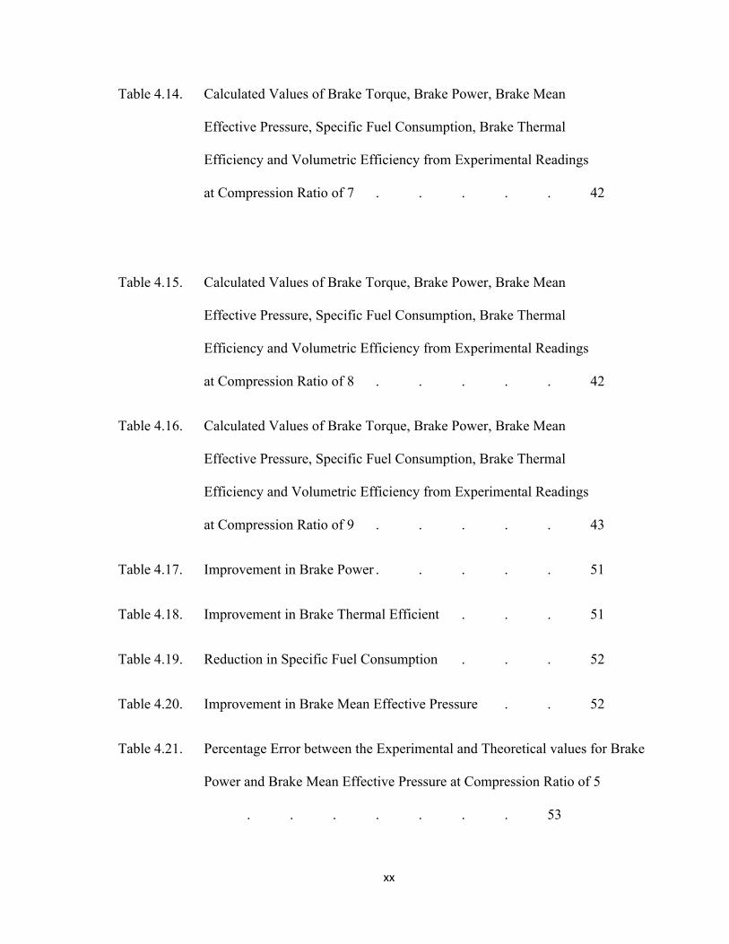
Table 4.14. Calculated Values of Brake Torque, Brake Power, Brake Mean
Effective Pressure, Specific Fuel Consumption, Brake Thermal
Efficiency and Volumetric Efficiency from Experimental Readings
at Compression Ratio of 7 . . . . . 42
Table 4.15. Calculated Values of Brake Torque, Brake Power, Brake Mean
Effective Pressure, Specific Fuel Consumption, Brake Thermal
Efficiency and Volumetric Efficiency from Experimental Readings
at Compression Ratio of 8 . . . . . 42
Table 4.16. Calculated Values of Brake Torque, Brake Power, Brake Mean
Effective Pressure, Specific Fuel Consumption, Brake Thermal
Efficiency and Volumetric Efficiency from Experimental Readings
at Compression Ratio of 9 . . . . . 43
Table 4.17. Improvement in Brake Power . . . . . 51
Table 4.18. Improvement in Brake Thermal Efficient . . . 51
Table 4.19. Reduction in Specific Fuel Consumption . . . 52
Table 4.20. Improvement in Brake Mean Effective Pressure . . 52
Table 4.21. Percentage Error between the Experimental and Theoretical values for Brake
Power and Brake Mean Effective Pressure at Compression Ratio of 5
. . . . . . . 53
xxi
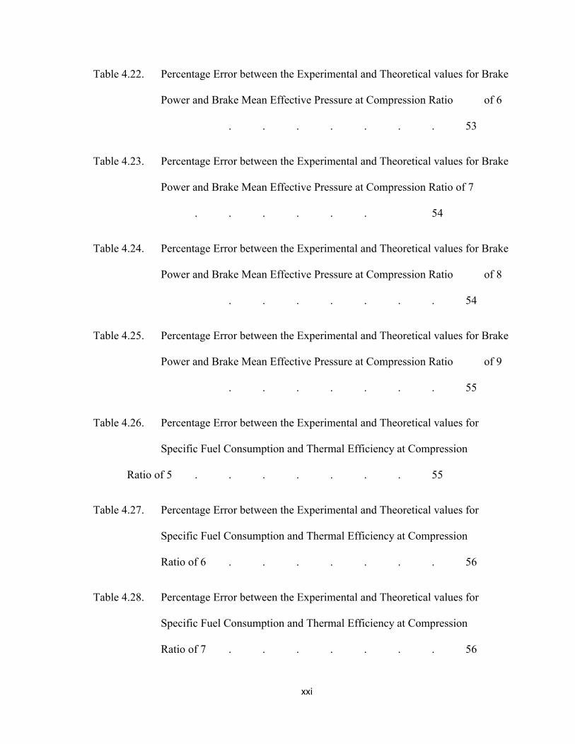
Table 4.22. Percentage Error between the Experimental and Theoretical values for Brake
Power and Brake Mean Effective Pressure at Compression Ratio of 6
. . . . . . . 53
Table 4.23. Percentage Error between the Experimental and Theoretical values for Brake
Power and Brake Mean Effective Pressure at Compression Ratio of 7
. . . . . . 54
Table 4.24. Percentage Error between the Experimental and Theoretical values for Brake
Power and Brake Mean Effective Pressure at Compression Ratio of 8
. . . . . . . 54
Table 4.25. Percentage Error between the Experimental and Theoretical values for Brake
Power and Brake Mean Effective Pressure at Compression Ratio of 9
. . . . . . . 55
Table 4.26. Percentage Error between the Experimental and Theoretical values for
Specific Fuel Consumption and Thermal Efficiency at Compression
Ratio of 5 . . . . . . . 55
Table 4.27. Percentage Error between the Experimental and Theoretical values for
Specific Fuel Consumption and Thermal Efficiency at Compression
Ratio of 6 . . . . . . . 56
Table 4.28. Percentage Error between the Experimental and Theoretical values for
Specific Fuel Consumption and Thermal Efficiency at Compression
Ratio of 7 . . . . . . . 56
xxii
Table 4.29. Percentage Error between the Experimental and Theoretical values for
Specific Fuel Consumption and Thermal Efficiency at Compression
Ratio of 8 . . . . . . . 57
Table 4.30. Percentage Error between the Experimental and Theoretical values for
Specific Fuel Consumption and Thermal Efficiency at Compression
Ratio of 9 . . . . . . . 57
Table 5.1. Grand Averages of the Percentage Error . . . 84
xxiii
LIST OF PLATES
Plate 2.1 The piston, with the 15:1 compression ratio crown assembled of a
natural gas HCCI engine . . . . . 13
Plate 3.1 Ricardo E6/T variable compression ratio single cylinder four stroke
petrol engine . . . . . . . 22
Plate 3.2 Dynamometer of the Ricardo variable compression ratio engine 24
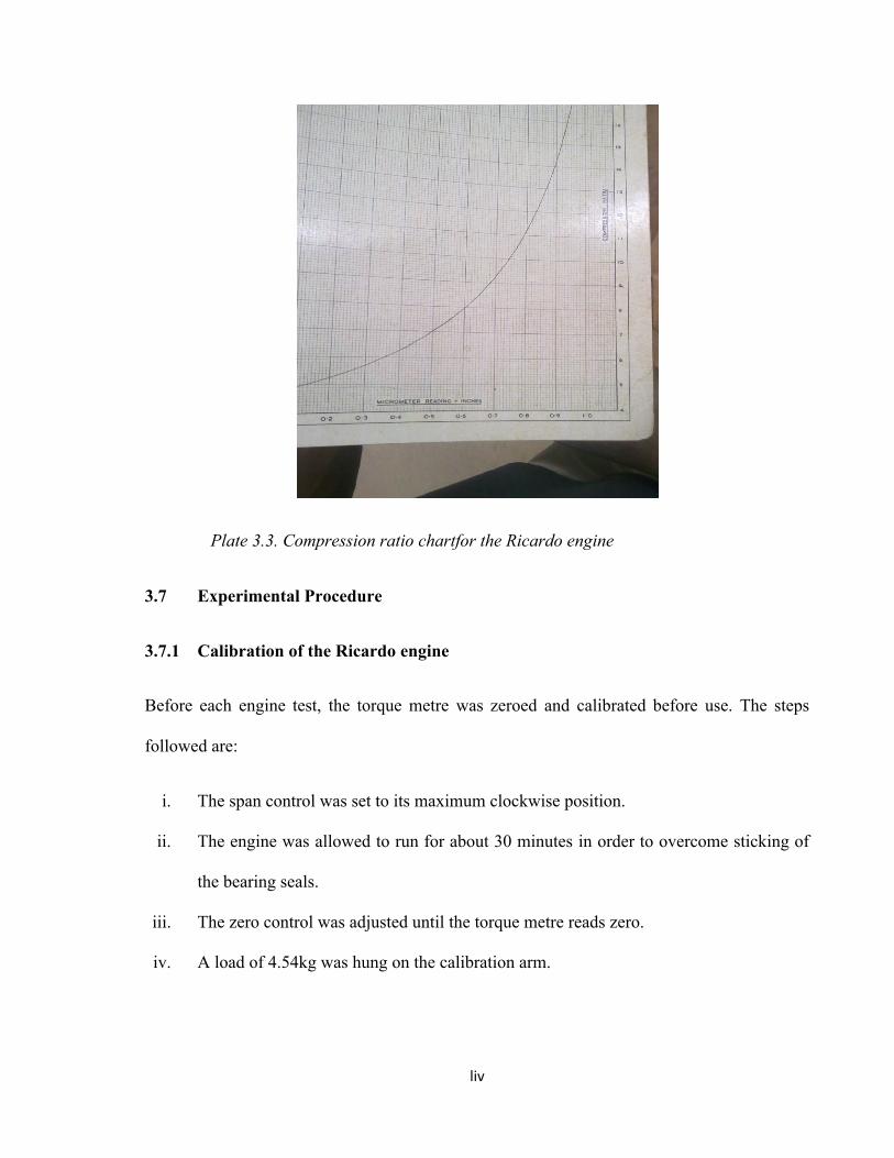
Plate 3.3 Compression ratio chart for the Ricardo engine . . 29
xxiv
LIST OF APPENDICES
Appendix A. Engineering Equation Solver (EES) computer programme
(Modelled equations for experimental analysis) . . 90
Appendix B. Engineering Equation Solver (EES) computer programme (Modelled equations
for theoretical analysis) . . . 100
Appendix C. Formatted Equations for Experimental Analysis . . 110
Appendix D. Formatted Equations for Theoretical Analysis . . 125
xxv
ABBREVIATIONS AND SYMBOLS
ABBREVIATIONS
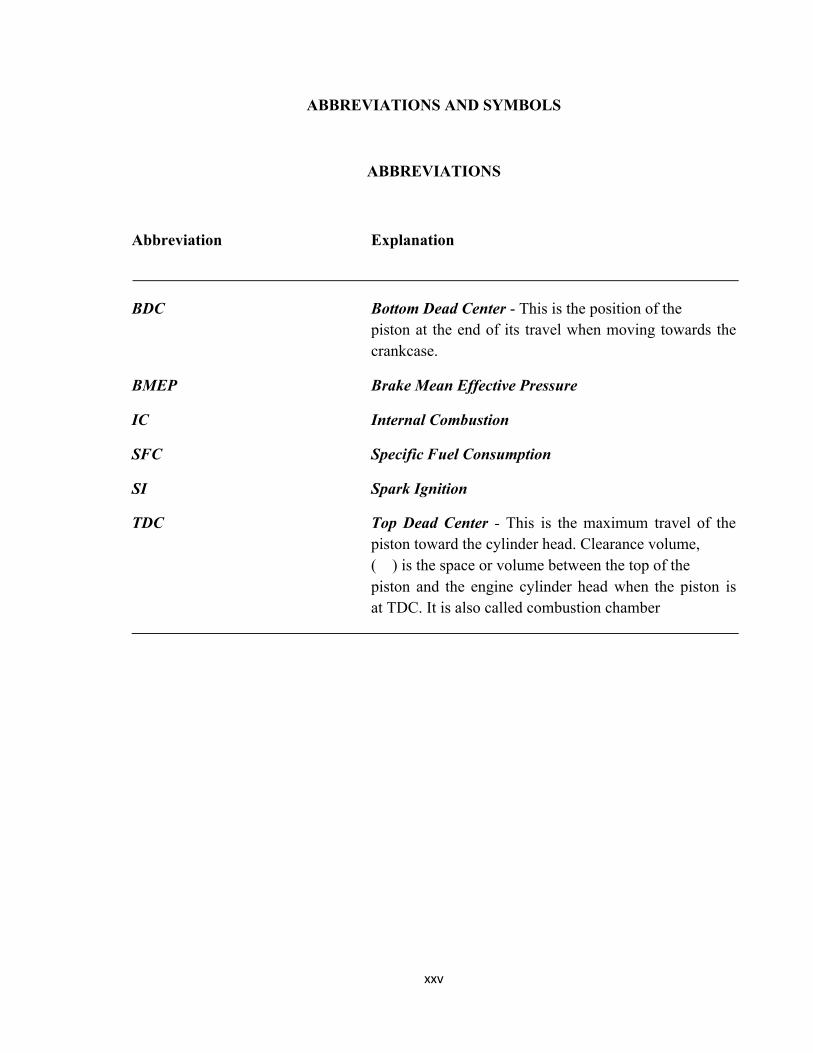
Abbreviation Explanation
BDC Bottom Dead Center - This is the position of the piston at the end of its travel when moving towards the crankcase.
BMEP Brake Mean Effective Pressure
IC Internal Combustion
SFC Specific Fuel Consumption
SI Spark Ignition
TDC Top Dead Center - This is the maximum travel of thepiston toward the cylinder head. Clearance volume, ( ) is the space or volume between the top of the piston and the engine cylinder head when the piston is at TDC. It is also called combustion chamber
xxvi
SYMBOLS
A Piston Area (mm2)
A0 Orifice area (m2)
B Cylinder Bore (mm)
Brake power (kW)
Discharge coefficient
g Acceleration due to gravity (m/s2)
h Manometer reading (mm-water)
L Cylinder Stroke length (mm)
Mass flow rate of air (kg/s)
Mass flow rate of fuel (kg/s)
Engine Speed (rpm)
n Number of Cylinders
Volumetric flow rate (m3/s)
Lower calorific value of the fuel (kJ/kg K)
Compression Ratio
Gas constant (kJ/kg K)
R Torque Arm (m)
S Cylinder Stroke (mm)
Specific gravity of the fuel
t Time (sec)
Torque (Nm)
Swept Volume (mm3)
Volume of the fuel consumed (m3)
xxvii
Vc Clearance volume (m3)
W Brake Load (N)
Air density (kg/m3)
Water density (kg/m3)
Brake Thermal Efficiency (%)
Volumetric Efficiency (%)
xxviii
CHAPTER ONE
INTRODUCTION
The internal combustion (IC) engine has been refined and developed over the last 100 years
for a wide variety of applications. In most application of power generation and in
transportation propulsion the power source has being the internal combustion engines. The
reciprocating engine with its compact size and its wide range of power outputs and fuel
options is an ideal prime mover for powering cars, trucks, off-highway vehicles, trains, ships,
motor bikes as well aselectrical power generators for a wide range of large and small
applications. Electricity generating sets used to provide primary power in remote locations or
more generally for providing mobile and emergency or stand-by electrical power utilizes the
IC engines (Piston engine power plant, 2005). In Germany, Dr. Nicolaus August Otto started
manufacturing gas engines in 1866 (Hillier and Pittuck, 1978).
The IC engine is a heat engine in which burning of a fuel occurs in a confined space called a
combustion chamber. This exothermic reaction of a fuel with an oxidizer creates gases of high
temperature and pressure which are permitted to expand. The defining feature of an IC engine
is that useful work is performed by the expanding hot gases acting directly to cause
movement, for example by acting on piston, rotor, or even by pressing on and moving the
entire engine itself (Singer and Raper, 1999).
1.1 Advantages and Applications of Internal Combustion Engines
xxix
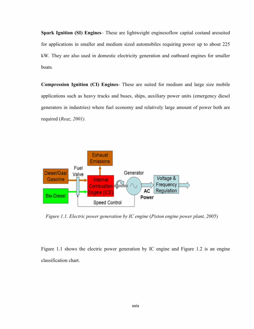
Spark Ignition (SI) Engines– These are lightweight enginesoflow capital costand aresuited
for applications in smaller and medium sized automobiles requiring power up to about 225
kW. They are also used in domestic electricity generation and outboard engines for smaller
boats.
Compression Ignition (CI) Engines- These are suited for medium and large size mobile
applications such as heavy trucks and buses, ships, auxiliary power units (emergency diesel
generators in industries) where fuel economy and relatively large amount of power both are
required (Reaz, 2001).
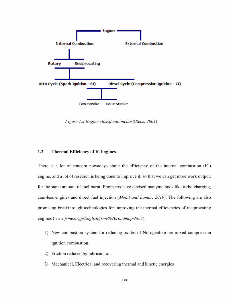
Figure 1.1 shows the electric power generation by IC engine and Figure 1.2 is an engine
classification chart.
Figure 1.1. Electric power generation by IC engine (Piston engine power plant, 2005)
xxx
Figure 1.2.Engine classificationchart(Reaz, 2001)
1.2 Thermal Efficiency of ICEngines
There is a lot of concern nowadays about the efficiency of the internal combustion (IC)
engine, and a lot of research is being done to improve it, so that we can get more work output,
for the same amount of fuel burnt. Engineers have devised manymethods like turbo charging,
cam-less engines and direct fuel injection (Mohit and Lamar, 2010). The following are also
promising breakthrough technologies for improving the thermal efficiencies of reciprocating
engines (www.jsme.or.jp/English/jsme%20roadmap/N0.7):
1) New combustion system for reducing oxides of Nitrogenlike pre-mixed compression
ignition combustion.
2) Friction reduced by lubricant oil.
3) Mechanical, Electrical and recovering thermal and kinetic energies
xxxi
4) Transfer from fossil fuel to biomass fuel
The fuel cell is an important breakthrough technology currently under examination. It
is expected to be put into practical use from 2015 to 2020.
The thermal efficiency of the working cycle characterizes the degree of perfection with which
heat is converted into work. The thermal efficiency is the ratio of the energy output at the
shaft to input energy from the fuel. Of all the energy present in the combustion chamber only
some gets converted to useful output power. Most of the energy produced by these engines is
wasted as heat. The average IC engine has thermal efficiency between 20 to 30%, which is
very low (Mohit and Lamar, 2010).
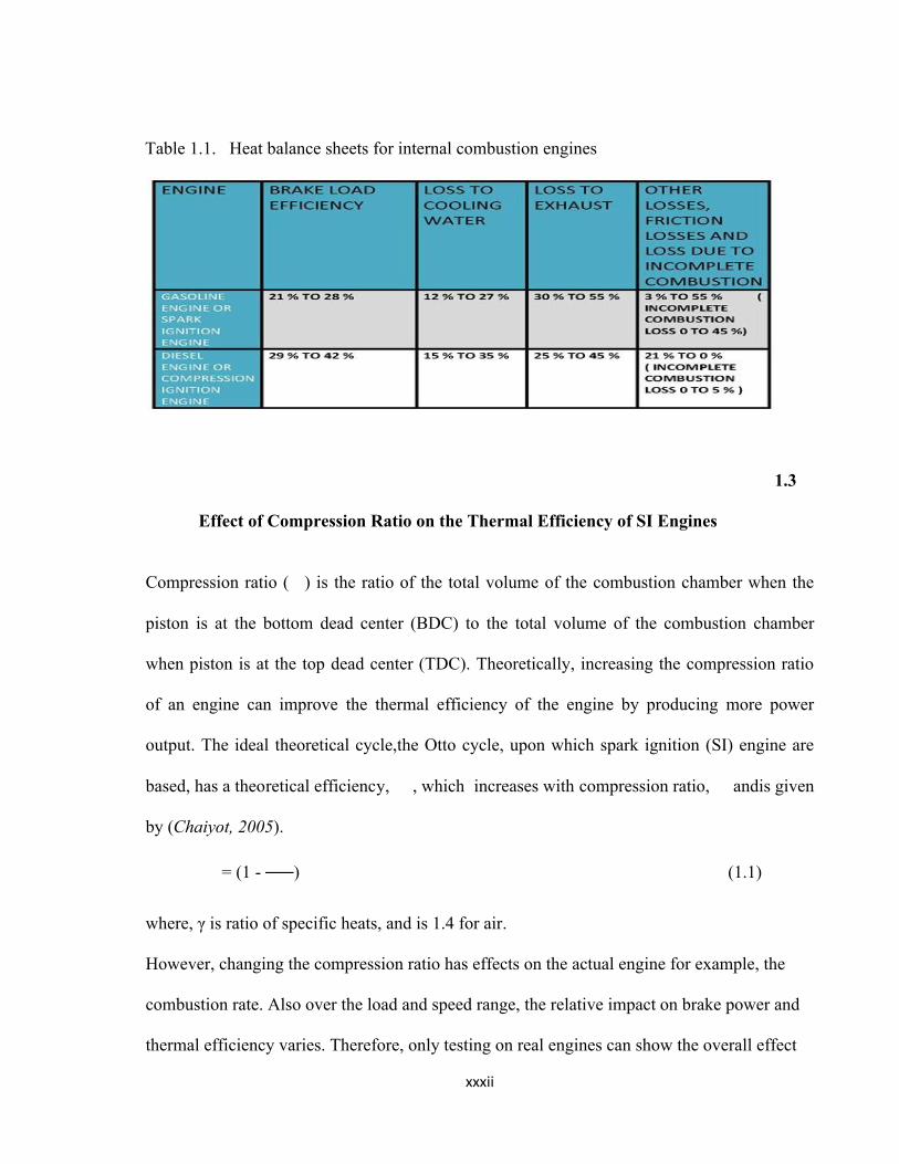
If we consider a heat balance sheetsby Mohits and Lamar (2010) for the internal combustion
engines for a spark ignition (gasoline) engine, we find that the brake load efficiency is
between 21 to 28%, whereas loss to cooling water is between 12 to 27%, loss to exhaust is
between 30 to 55 %, and loss due to incomplete combustion is between 0 to 45%.By
analyzing the heat balance sheet we find that in gasoline engines loss due to incomplete
combustion can be rather high leading to poor performance characteristics of the engine.
In addition to friction losses and losses to the exhaust there are other engine operating
parameters that affect thermal efficiency. These include the fuel calorific value, the
compression ratio, and the ratio of specific heats, (γ= / ).
xxxii
1.3
Effect of Compression Ratio on the Thermal Efficiency of SI Engines
Compression ratio ( ) is the ratio of the total volume of the combustion chamber when the
piston is at the bottom dead center (BDC) to the total volume of the combustion chamber
when piston is at the top dead center (TDC). Theoretically, increasing the compression ratio
of an engine can improve the thermal efficiency of the engine by producing more power
output. The ideal theoretical cycle,the Otto cycle, upon which spark ignition (SI) engine are
based, has a theoretical efficiency, , which increases with compression ratio, andis given
by (Chaiyot, 2005).
= (1 - ) (1.1)
where, γ is ratio of specific heats, and is 1.4 for air.
However, changing the compression ratio has effects on the actual engine for example, the
combustion rate. Also over the load and speed range, the relative impact on brake power and
thermal efficiency varies. Therefore, only testing on real engines can show the overall effect
Table 1.1. Heat balance sheets for internal combustion engines
xxxiii
of the compression ratio. Knocking, however, is a limitation for increasing the compression
ratio (Chaiyot, 2005).
1.4 Statement of the Problem
The electricity power generation by Power Holding Company of Nigeria (PHCN)
amount to about 3,700 MW, which is lower than the national demand of about 10,000 MW
(www.sweetcrudereports.com/2011/power). This implies that PHCN meets less than 50% of
the national demand. This has therefore necessitated establishments and families to generate
their own electricity using small engines. Most of these engines that are bought off-shelf (in
the market) are designed with a fixed compression ratio. These engines are to operate at
maximum thermal efficiency or lowest specific fuel consumption.
The thermal efficiency, of the Otto cycle on which spark ignition engines are based is
given by equation (1). This implies that thermal efficiency is dependent on compression ratio
and ratio of specific heats. Compression ratio is a fundamental parameter in determining the
thermal efficiency of the engine.For spark ignition (SI) engines, the compression ratio ranges
from 6 to 12 (Haresh and Swagatam 2008). As a general rule, the energy in the fuel will be
better utilized if the compression ratio is as high as possible within the detonation free range.
xxxiv
1.5 The Present Research
This work attempts to investigate for a giving four stroke Spark Ignition engine, the influence
of compression ratio on the brake thermal efficiency, brake power, brake mean effective
pressure, specific fuel consumption, and the economic benefits for each unit increase in
compression ratio from 5 to 9; which is within detonation free range for spark ignition
engines.
The concern is for us to ensure that smaller engines such as the generators that we use in the
homes are fuel efficient, designed for optimum thermal efficiency within detonation free
compression ratios in order to reduce the cost of our supplementing electricity power supply
from PHCN.
1.6 Aim and Objectives
The aim of the research is to determine experimentally and theoretically, the influence of the
compression ratios on the performance characteristics of a spark ignition engine.
The specific objectives of this research are as follows
(i) To determine experimentally the influence of compression ratio on:
a. brake power
b. brake mean effective pressure
c. brake thermal efficiency
d. specific fuel consumption.
xxxv
(ii) To test the level of agreement of theoretical predictionswith derived performance
characteristics equationsto predict theoretically,the influence of compression ratio
on performance characteristics, a to d in (i)
1.7 Significance of Research
Adopting a higher compression ratio is one of the most important considerations regarding
improved fuel consumption, thermal efficiency and power output in gasoline engines. Much
research has been devoted to the effect of higher compression ratio in compression ignition
engines, but little attention has been given to spark engines because of detonation at higher
compression ratios. By far the most widely used IC engine is the spark-ignition gasoline
engine (www.personal.utulsa.edu/kenneth-weston/chapter6.pdf). A four-stroke SI engine is
different from a four-stroke CI engine in the combustion process and in the, pressure and
temperature characteristics of the working gases. The compression ratio has a significant
effect on the thermal efficiency for the respective engine types.
xxxvi
CHAPTER TWO
LITERATURE REVIEW
A lot of research has beendone to improve the performance of internal combustion engines.
Below are some of the past works.
2.1 Review of Related Past Works
iAsifet at. (2008) conducted a research on performance evaluation of a single cylinder four
stroke petrol engine. In the research, the actual size of the engine parameters like the bore,
stroke, swept volume, clearance volume, compression ratio and engine speed were
recorded and computed. Based on the actual size of the engine parameters, the indicated
horse power, brake power, and friction horse power were determined and were found to be
1.54, 1.29 and 0.25 respectively. The mechanical efficiency and the thermal efficiency
were also calculated and were found to be 83% and 20.5% respectively. The fuel
consumption per hour was found to be 0.8 litre/hour while the fuel consumption per
distance traveled was found to be 60 km/litre.
iiOwoade (1971) conducted a research on the performance of a variable compression ratio SI
engine at full throttle. The research was conducted for compression ratios of 8, 9, 10 and
11. It was observedthat a compression ratio of 10.5 gave the maximum brake horse power.
Above this value (compression ratio of 10.5), there was a decrease in brake horse power at
xxxvii
each ignition setting. Also, the values for the thermal efficiency for both the hypothetical
and actual engine increased with the compression ratio
iiiYuh and Tohru (2005) carried out a research on the effect of higher compression ratio in
two-stroke engines. The results showed that the actual fuel consumption improved by 1-
3% for each unit increase in the compression ratio range of 6.6 to 13.6. It was observed
that the rate of improvement was smaller as compared to the theoretical values. The
discrepancies were mainly due to increased mechanical and cooling losses, short-
circuiting at low loads and increased time losses at heavy loads. Power output also
improved, but the maximum compression ratio was limited due to knock and the increase
in thermal load. In addition, the investigation covered the implementation of higher
compression ratio in practical engines by retarding the full-load ignition timing.
ivAbdel and Osman (1997) performed an experimental investigation on varying the
compression ratio of spark ignition engines working under different ethanol-gasoline fuel
blends.. The result showed that the engine indicated power improved with the percentage
addition of the ethanol in the fuel blend. The maximum improvement occurred at 10%
ethanol-90% gasoline fuel blends.
vChaiyotet al. (2005) conducted an experimental study on influence of compression ratio on
the performance and emission of compressed natural gas (CNG) retrofit engine. For the
engine testing, CNG dedicated engine was tested at 4 compression ratios of 9, 9.5, 10, and
10.5. The engine testing schematic diagram is shown in Figure 2.1
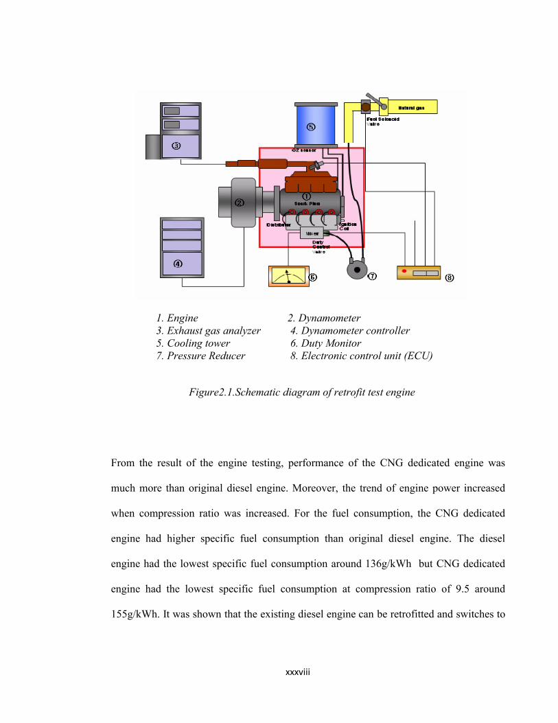
xxxviii
1. Engine 2. Dynamometer3. Exhaust gas analyzer 4. Dynamometer controller5. Cooling tower 6. Duty Monitor7. Pressure Reducer 8. Electronic control unit (ECU)
Figure2.1.Schematic diagram of retrofit test engine
From the result of the engine testing, performance of the CNG dedicated engine was
much more than original diesel engine. Moreover, the trend of engine power increased
when compression ratio was increased. For the fuel consumption, the CNG dedicated
engine had higher specific fuel consumption than original diesel engine. The diesel
engine had the lowest specific fuel consumption around 136g/kWh but CNG dedicated
engine had the lowest specific fuel consumption at compression ratio of 9.5 around
155g/kWh. It was shown that the existing diesel engine can be retrofitted and switches to
xxxix
use CNG asalternative fuel which results on money saving, more power output and clean
emissions.
viJan-Ola et al. (2002) carried out a research on the compression ratio influence on
maximum load of a Natural Gas HCCI engine.A Volvo TD100 truck engine was used for
the experiment. The engine was controlled in a closed-loop fashion by enriching the
Natural Gas mixture with Hydrogen. The first section of the paper illustrated and
discussed the potential of using hydrogen enrichment of natural gas to control
combustion timing. Full-cycle simulation was carried out and compared to some of the
experimental data and then used to enhance some of the experimental observations
dealing with ignition timing, thermal boundary conditions, emissions and how they affect
engine stability and performance. High load issues common to HCCI were discussed in
light of the inherent performance and emissions tradeoff and the disappearance of
feasible operating space at high engine loads. The problems of tighter limits for
combustion timing, unstable operational points and physical constraints at high loads
were discussed and illustrated by experimental results. It was concluded that the
operational limits were affected by compression ratio at high load, based on the criteria
discussed in the second part.
xl
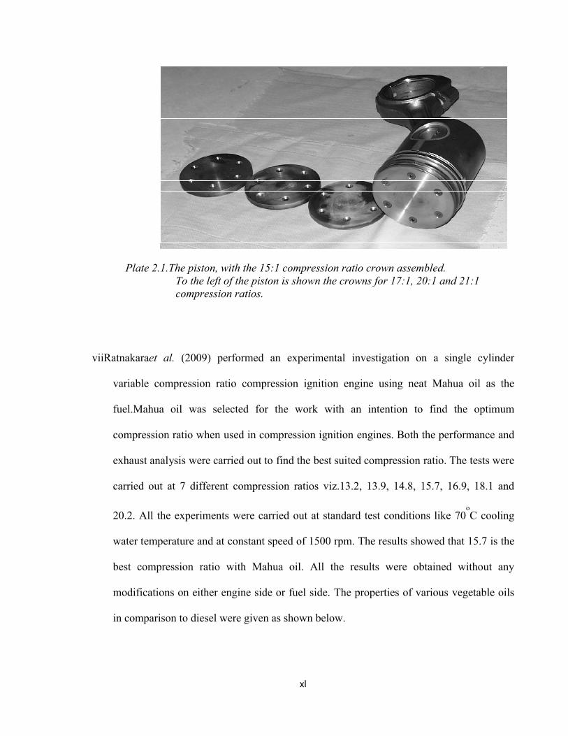
Plate 2.1.The piston, with the 15:1 compression ratio crown assembled. To the left of the piston is shown the crowns for 17:1, 20:1 and 21:1
compression ratios.
viiRatnakaraet al. (2009) performed an experimental investigation on a single cylinder
variable compression ratio compression ignition engine using neat Mahua oil as the
fuel.Mahua oil was selected for the work with an intention to find the optimum
compression ratio when used in compression ignition engines. Both the performance and
exhaust analysis were carried out to find the best suited compression ratio. The tests were
carried out at 7 different compression ratios viz.13.2, 13.9, 14.8, 15.7, 16.9, 18.1 and
20.2. All the experiments were carried out at standard test conditions like 70oC cooling
water temperature and at constant speed of 1500 rpm. The results showed that 15.7 is the
best compression ratio with Mahua oil. All the results were obtained without any
modifications on either engine side or fuel side. The properties of various vegetable oils
in comparison to diesel were given as shown below.
xli
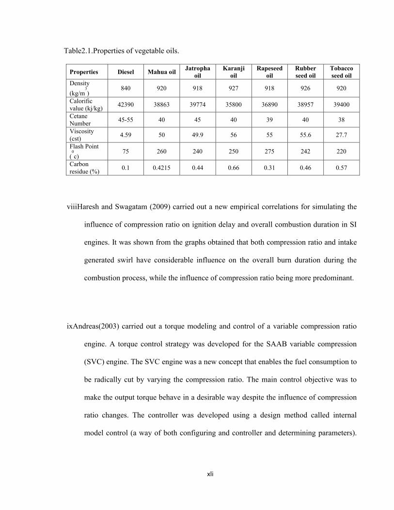
Table2.1.Properties of vegetable oils.
viiiHaresh and Swagatam (2009) carried out a new empirical correlations for simulating the
influence of compression ratio on ignition delay and overall combustion duration in SI
engines. It was shown from the graphs obtained that both compression ratio and intake
generated swirl have considerable influence on the overall burn duration during the
combustion process, while the influence of compression ratio being more predominant.
ixAndreas(2003) carried out a torque modeling and control of a variable compression ratio
engine. A torque control strategy was developed for the SAAB variable compression
(SVC) engine. The SVC engine was a new concept that enables the fuel consumption to
be radically cut by varying the compression ratio. The main control objective was to
make the output torque behave in a desirable way despite the influence of compression
ratio changes. The controller was developed using a design method called internal
model control (a way of both configuring and controller and determining parameters).
Properties Diesel Mahua oil Jatropha
oil Karanji
oil Rapeseed
oil Rubber seed oil
Tobacco seed oil
Density
(kg/m3)
840 920 918 927 918 926 920
Calorific value (kj/kg)
42390 38863 39774 35800 36890 38957 39400
Cetane Number
45-55 40 45 40 39 40 38
Viscosity (cst)
4.59 50 49.9 56 55 55.6 27.7
Flash Point
(0c)
75 260 240 250 275 242 220
Carbon residue (%)
0.1 0.4215 0.44 0.66 0.31 0.46 0.57
xlii
The controller was implemented andevaluated in a real engine. The controller was
proved to reduce the effects from compression ratio changes.
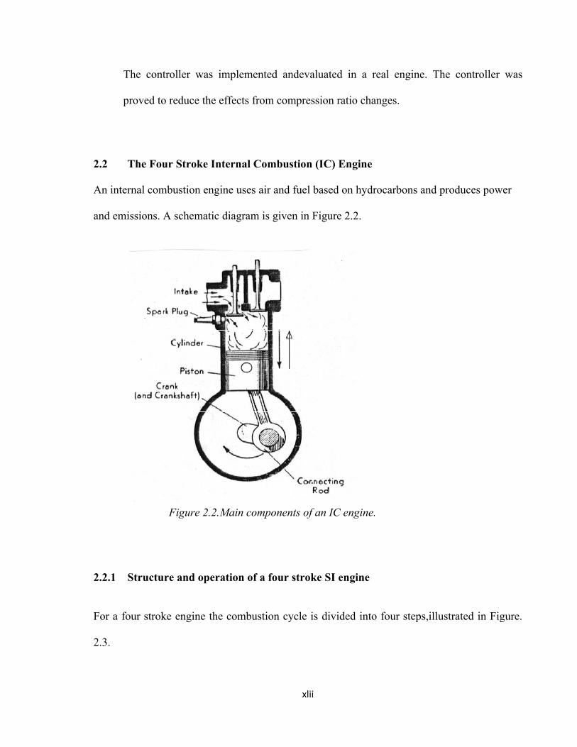
2.2 The Four Stroke Internal Combustion (IC) Engine
An internal combustion engine uses air and fuel based on hydrocarbons and produces power
and emissions. A schematic diagram is given in Figure 2.2.
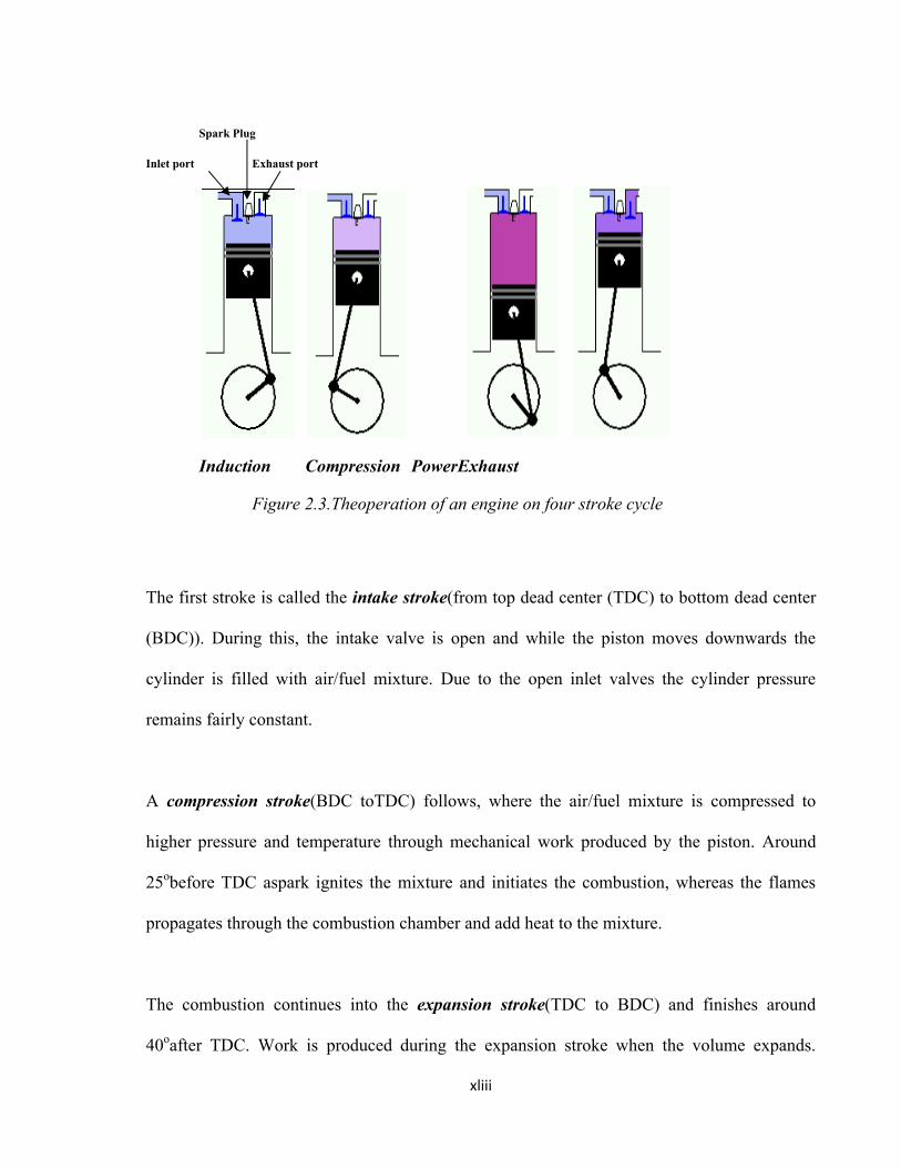
2.2.1 Structure and operation of a four stroke SI engine
For a four stroke engine the combustion cycle is divided into four steps,illustrated in Figure.
2.3.
Figure 2.2.Main components of an IC engine.
xliii
Spark Plug
Inlet port Exhaust port
Induction Compression PowerExhaust
Figure 2.3.Theoperation of an engine on four stroke cycle
The first stroke is called the intake stroke(from top dead center (TDC) to bottom dead center
(BDC)). During this, the intake valve is open and while the piston moves downwards the
cylinder is filled with air/fuel mixture. Due to the open inlet valves the cylinder pressure
remains fairly constant.
A compression stroke(BDC toTDC) follows, where the air/fuel mixture is compressed to
higher pressure and temperature through mechanical work produced by the piston. Around
25obefore TDC aspark ignites the mixture and initiates the combustion, whereas the flames
propagates through the combustion chamber and add heat to the mixture.
The combustion continues into the expansion stroke(TDC to BDC) and finishes around
40oafter TDC. Work is produced during the expansion stroke when the volume expands.
xliv
Around 130o after TDC the exhaust valve is opened and the blow down process starts, where
the cylinder pressure decreases as the burned gases is blown out into the exhaust system by
the higher pressure in the cylinder.
During the final stroke, exhaust stroke(BDC to TDC), the valve is still open and therefore the
pressure in the cylinder is close to the pressure in the exhaust system and the rest of the gases
is pushed out into the exhaust system as the piston moves upwards. When the piston reaches
TDC a new cycle starts with the intake stroke (Andreas, 2003).
2.3 Engine Performance Parameters
The term ‘’performance’’ usually means how well an engine is doing its required task of
converting the input energy to useful energy. It is represented by typical characteristics
curves, which show an engine’s performance.
Engine performance characteristics can be determined by the following two methods (Jehad
and Mohammed, 2003):
i. Experimental results obtained from engine tests.
ii. Analytical calculations.
Performance evaluation of SI engines is of great importance for their economic operation.
Some of the methods for assessing the engine performance include the determination of the
engine brake power, thermal efficiency, specific fuel consumption, considering the
compression ratio, the engine speed, and the brake mean effective pressure (Asif et al, 2008)
xlv
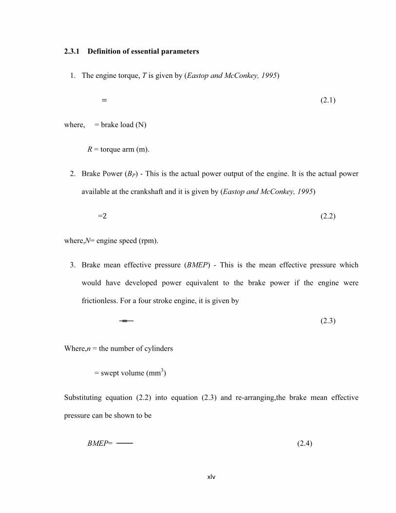
2.3.1 Definition of essential parameters
1. The engine torque, T is given by (Eastop and McConkey, 1995)
= (2.1)
where, = brake load (N)
R = torque arm (m).
2. Brake Power (BP) - This is the actual power output of the engine. It is the actual power
available at the crankshaft and it is given by (Eastop and McConkey, 1995)
=2 (2.2)
where,N= engine speed (rpm).
3. Brake mean effective pressure (BMEP) - This is the mean effective pressure which
would have developed power equivalent to the brake power if the engine were
frictionless. For a four stroke engine, it is given by
= (2.3)
Where,n = the number of cylinders
= swept volume (mm3)
Substituting equation (2.2) into equation (2.3) and re-arranging,the brake mean effective
pressure can be shown to be
BMEP=
(2.4)
xlvi
therefore, Thisimplies that the brake mean effective pressure is directly proportional to the torque.
4. Brake thermal efficiency ( ) – This is the ratio of the brake power to the fuel power,
(heat supplied)
= (2.5)
and = (2.6)
where, = mass flow rate of the fuel(kg/s)
= lower calorific value of the fuel (kJ/kgK)
5. Specific Fuel Consumption (SFC) – This is the total fuel consumed per kilowatt power
developed per hour, in (kg/KW h) and it is given by (Eastop and McConkey, 1995).
SFC= 3600 (2.7)
Combining equations (2.5) and (2.7), the specific fuel consumption can be shown to be
SFC = (2.8)
therefore,SFC 1
This shows that specific fuel consumption is inversely proportional to the thermal efficiency.
6. Volumetric efficiency ( ) –Andreas (2003) shows that the air mass flow passing the
intake valve, depends mainly on the engine speed, intake manifold pressure and air
xlvii
temperature.The volumetric efficiency is a measure of the effectiveness of the engine to
induced fresh air defined as the ratio of actual volume flow rate of air entering the
cylinder ( ⁄ ), and the rate at which volume is displayed by the piston, . The
factor 2 in the denominator arises from the fact that the engine only induced fresh air in
the cylinder every second revolution in a four stroke cycle. Using the above, the
expression for the volumetric efficiency becomes
= / (2.9)
7. Compression ratio ( ) - Compression ratio by Eastop and McConkey(1995) is giving by
=
(2.10)
where, = Cylinder clearance volume (m3)
The compression ratio is one of the most important factors that determine how efficient the
engine can utilize the energy in the fuel (equation(1)). As a general rule, the energy in the fuel
will be better utilized ifthe compression ratio is as high as possible.
From equation (2.10), the swept volume can be shown to be
= ( -1) (2.11)
Substituting equation (2.11) into (2.9), the volumetric efficiency in terms of the compression
ratio and clearance volume can be shown to be
= ( −1) / (2.12)
xlviii
CHAPTER THREE
MATERIALS AND METHODS
3.1 Description of Test Engine
In this section, a description of the testengineis given,and the major specifications.The
experimental procedures andtheoretical determination of the performance characteristicsare
also presented.
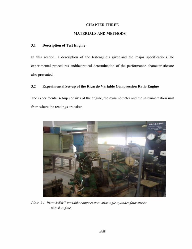
3.2 Experimental Set-up of the Ricardo Variable Compression Ratio Engine
The experimental set-up consists of the engine, the dynamometer and the instrumentation unit
from where the readings are taken.
Plate 3.1. RicardoE6/T variable compressionratiosingle cylinder four stroke petrol engine.
3.3 The Engine
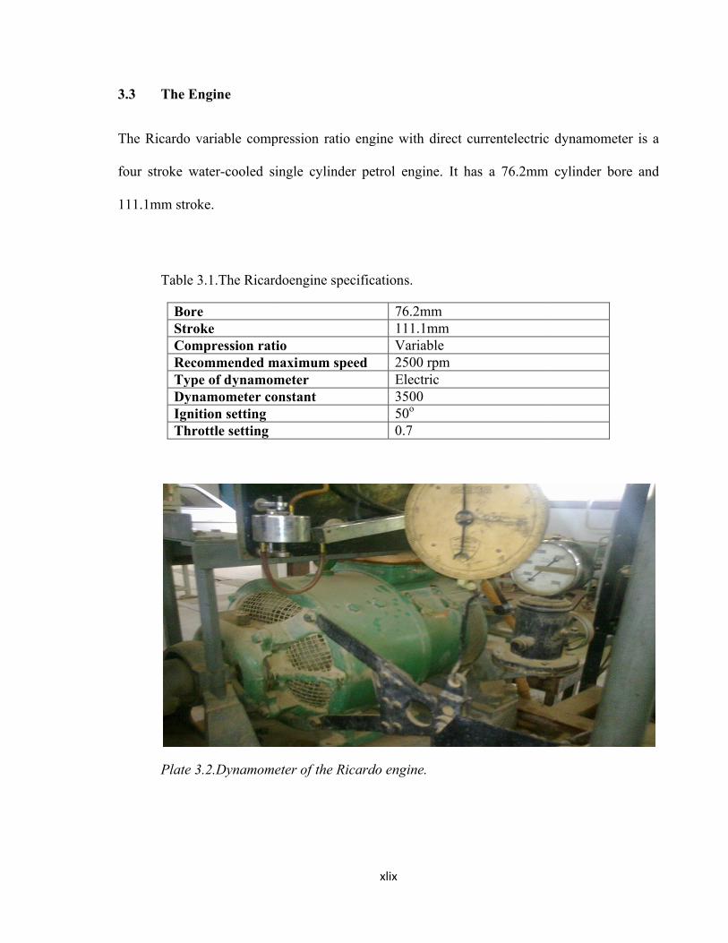
The Ricardo variable compression ratio engine with direct currentelectric dynamometer is a
four stroke water-cooled single cylinder petrol engine. It has a 76.2mm cylinder bore and
111.1mm stroke.
Table 3.1.The Ricardoengine s
BoreStrokeCompression ratioRecommended maximum speedType of dynamometerDynamometer constantIgnition settingThrottle setting
Plate 3.2.Dynamometer of the Ricardo e
xlix
variable compression ratio engine with direct currentelectric dynamometer is a
cooled single cylinder petrol engine. It has a 76.2mm cylinder bore and
Table 3.1.The Ricardoengine specifications.
76.2mm 111.1mm
Compression ratio VariableRecommended maximum speed 2500 rpmType of dynamometer ElectricDynamometer constant 3500
50o
0.7
3.2.Dynamometer of the Ricardo engine.
variable compression ratio engine with direct currentelectric dynamometer is a
cooled single cylinder petrol engine. It has a 76.2mm cylinder bore and
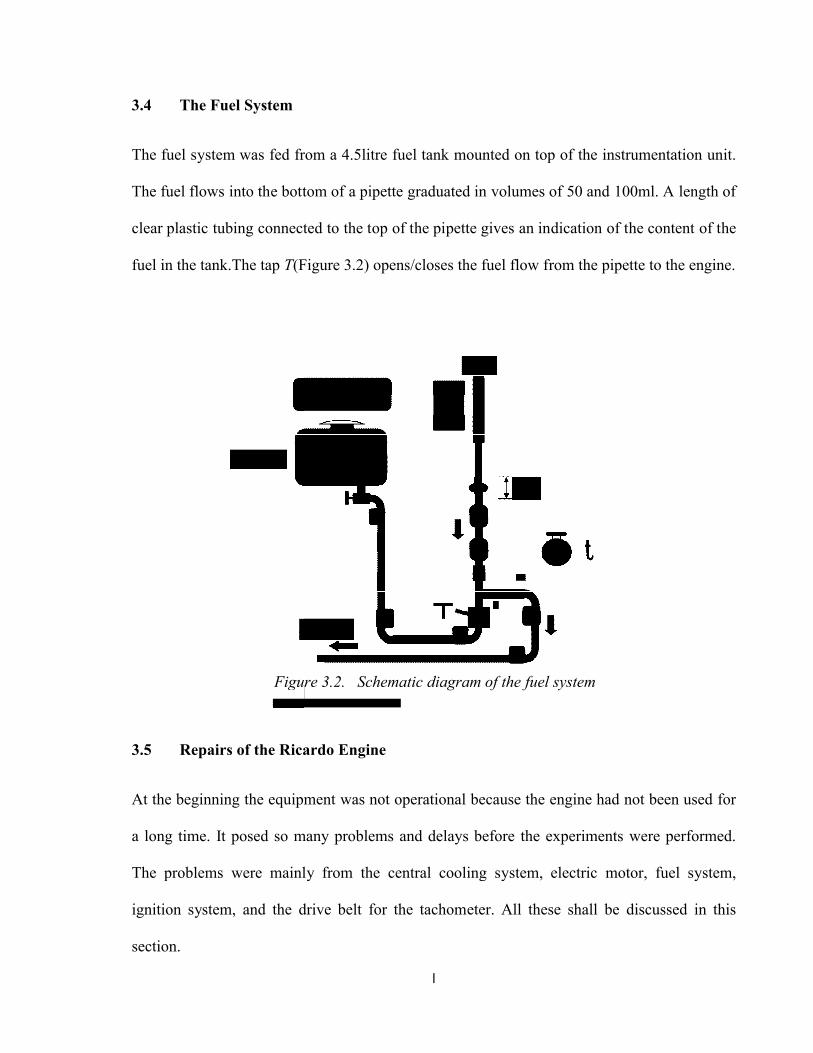
3.4 The Fuel System
The fuel system was fed from a 4.5litre fuel tank mounted on top of the instrumentation un
The fuel flows into the bottom of a pipette graduated in volumes of 50 and 100ml. A length of
clear plastic tubing connected to the top of the pipette gives an in
fuel in the tank.The tap T(Figure 3.2)
3.5 Repairs of the Ricardo
At the beginning the equipment was not operational because the engine had not been used
a long time. It posed so many problems and delays before the experiments were performed.
The problems were mainly from the central cooling system, electric motor, fuel system,
ignition system, and the drive belt for the tachometer. All these shall be
section.
Figure 3.2. Schematic
l
s fed from a 4.5litre fuel tank mounted on top of the instrumentation un
The fuel flows into the bottom of a pipette graduated in volumes of 50 and 100ml. A length of
clear plastic tubing connected to the top of the pipette gives an indication of the content of the
(Figure 3.2) opens/closes the fuel flow from the pipette to the engine.
icardo Engine
At the beginning the equipment was not operational because the engine had not been used
a long time. It posed so many problems and delays before the experiments were performed.
The problems were mainly from the central cooling system, electric motor, fuel system,
ignition system, and the drive belt for the tachometer. All these shall be
Figure 3.2. Schematic diagram of the fuel system
s fed from a 4.5litre fuel tank mounted on top of the instrumentation unit.
The fuel flows into the bottom of a pipette graduated in volumes of 50 and 100ml. A length of
dication of the content of the
opens/closes the fuel flow from the pipette to the engine.
At the beginning the equipment was not operational because the engine had not been used for
a long time. It posed so many problems and delays before the experiments were performed.
The problems were mainly from the central cooling system, electric motor, fuel system,
ignition system, and the drive belt for the tachometer. All these shall be discussed in this
li
3.5.1 Repairs of the central cooling system into the laboratory
The original pump required to pump water into the laboratory was not functional, anirrigation
water pump was hiredto lift the water from the underground tank (lower tank) to the header
tank (upper tank); so that by gravity, it supplies the water on all the engines in the laboratory.
The cooling water pump attached to the Ricardo engine was serviced by cleaning of the
internal parts and the electrical circuits were replaced. This also made the supply of cooling
water to the engine possible.
3.5.2 Repairs on the electric motor
The bed cables and burnt fuses on the motor of the Ricardo engine were replaced. After these
repairs the motor came on.
3.5.3 Repairs of the fuel system
The fuel system was serviced by cleaning and replacing the lubricating oil. The carburetor and
fuel pump were serviced to make the supply of fuel to the engine possible. The air filter
placed on the carburetor requires that only clean air goes into the carburetor in order to
prevent choking. Therefore, it was necessary to service the air filter. This was done by
thorough cleaning of the air filter. The manometer system was serviced by cleaning and
changing the manometer fluid to paraffin fluid instead of water for better sensitivity.
lii
3.5.4 Repairs of the ignition system
The spark plug of the engine was changed to the conventional one because, the engine came
with a special plug that could not be obtained elsewhere except by ordering. All the plug
cables were also replaced with the conventional one.
3.5.5 Replacement of the conveyor belt for the tachometer
The conveyor belt for the tachometer was removed and changed to a new one because the
existing belt was weak and could not transmit the effect of the engine speed to the tachometer.
The tachometer measures the engine speed.
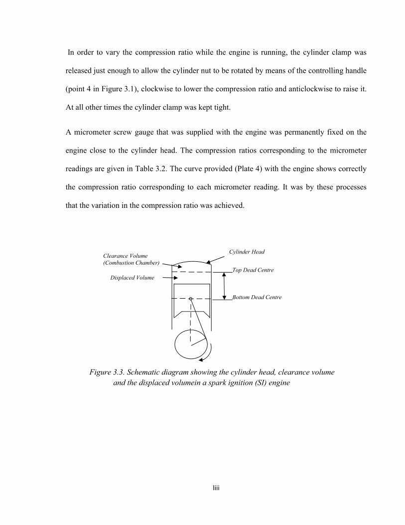
3.6 Variation of the Compression Ratio
Table 3.2.Compression ratios and corresponding micrometer readings.
Micrometre readings (mm) 0.135 0.36 0.503 0.605 0.697
Compression Ratio, 5 6 7 8 9
Variation of the compression ratio can be achieved byeither raising the cylinder head up in
order to decrease it or by lowering the cylinder head down to increase the compression
ratio.This can be understood clearly with Figure 3.3.
liii
In order to vary the compression ratio while the engine is running, the cylinder clamp was
released just enough to allow the cylinder nut to be rotated by means of the controlling handle
(point 4 in Figure 3.1), clockwise to lower the compression ratio and anticlockwise to raise it.
At all other times the cylinder clamp was kept tight.
A micrometer screw gauge that was supplied with the engine was permanently fixed on the
engine close to the cylinder head. The compression ratios corresponding to the micrometer
readings are given in Table 3.2. The curve provided (Plate 4) with the engine shows correctly
the compression ratio corresponding to each micrometer reading. It was by these processes
that the variation in the compression ratio was achieved.
Figure 3.3. Schematic diagram showing the cylinder head, clearance volume and the displaced volumein a spark ignition (SI) engine
Top Dead Centre
Bottom Dead Centre
Clearance Volume (Combustion Chamber)
Cylinder Head
Displaced Volume
liv
Plate 3.3. Compression ratio chartfor the Ricardo engine
3.7 Experimental Procedure
3.7.1 Calibration of the Ricardo engine
Before each engine test, the torque metre was zeroed and calibrated before use. The steps
followed are:
i. The span control was set to its maximum clockwise position.
ii. The engine was allowed to run for about 30 minutes in order to overcome sticking of
the bearing seals.
iii. The zero control was adjusted until the torque metre reads zero.
iv. A load of 4.54kg was hung on the calibration arm.
lv
v. The engine was started again by running it until the torque metre reading settles down
to a constant value.
vi. The span control was adjusted after which the torque reading was taken.
vii. The calibration load was removed and steps 1 to 6 were repeated until it was
satisfactory that the span settings were correct.
3.7.2 Test procedure
i. A throttle setting of 0.7 (as recommended) was selected. This was maintained
throughout the experiment.
ii. The needle valve controlling the strength of the mixture was maintained at one
position for each set of the compression ratios readings.
iii. The cylinder head was adjusted with the aid of the hand crank and micro-metre, and
the lowest possible compression ratio of 5.0 was obtained.
iv. The engine was started and the load adjusted to maintain the required speeds. The
lowest possible speed was 1100rpm, and it was increased in intervals of 100 from
1100rpm to 1600rpm. This speed range was maintained for each compression ratio.
v. The fuel consumption, air consumption and load on the dynamometer were taken and
recorded.
vi. Step (5) was repeated for various values of compression ratios, up to the highest
possible value, each time the load was adjusted to maintain the original speed. The
compression ratios were 5, 6, 7, 8, and 9.
lvi
vii. The mixture strength was varied and steps (3), (4), (5), and (6) were repeated.
3.8 Calculation of Mass Flow Rate of the Fuel
The fuel (petrol) consumption rate was determined by the time (t) taken by the engine to
consume 50ml of the fuel. The specific gravity of petrol is 0.74. The mass flow rate of the fuel
consumed is given by:
= φ (3.1)
And φ = (3.2)
Where, =specific gravity of the fuel (0.74)
= density of water (1000 kg/m3)
=volume of the fuel consumed (50ml = 5x10⁻⁵m3)
t = time (sec).
The time taken for the engine to consume 50ml of the fuel was 55.02 seconds, when the
compression ratio and engine speed were 5 and 1100 rpm respectively. Thus, applying
equation (3.1), the mass flow rate is given by
= 0.74 x 1000 x (
. ) = 0.0006725 kg/s
Similar calculations were carried out based on the time taken for the fuel to be consumed for
engine speeds of 1200, 1300, 1400, 1500 and 1600 rpm. The results are given in table
4.1.1 to 4.15 for compression ratios of 5, 6, 7, 8 and 9.
lvii
3.9 Measurement of Air Consumption
To calculate the flow rate of air passing through the orifice plate, the induction pipe was
connected to a large steel air cylinder-box by means of a hose. As the engine runs, air enters
the box through an orifice in the air box. An inclined manometer on the engine’s panel (point
11 in figure 3.1.) gives the pressure drop across the orifice; and hence the air consumption can
be calculated. The volumetric flow rate, Q for real flow is given by
(http://www.imnoeng.com/Flow/SmallOrificeGas.htm) Q =
∆(3.3)
Where, = discharge coefficient which depends on the Reynolds number of the airflow
(0.6 is a typical value)
= orifice area (m2)
∆P = drop in pressure
= air density
The mass flow rate of air, can be found by multiplying the volume flow rate, Q with the
air density, .
= Q (3.4)
Substituting for Q from equation (3.3) into equation (3.4),
= 2 ∆ (3.5)
lviii
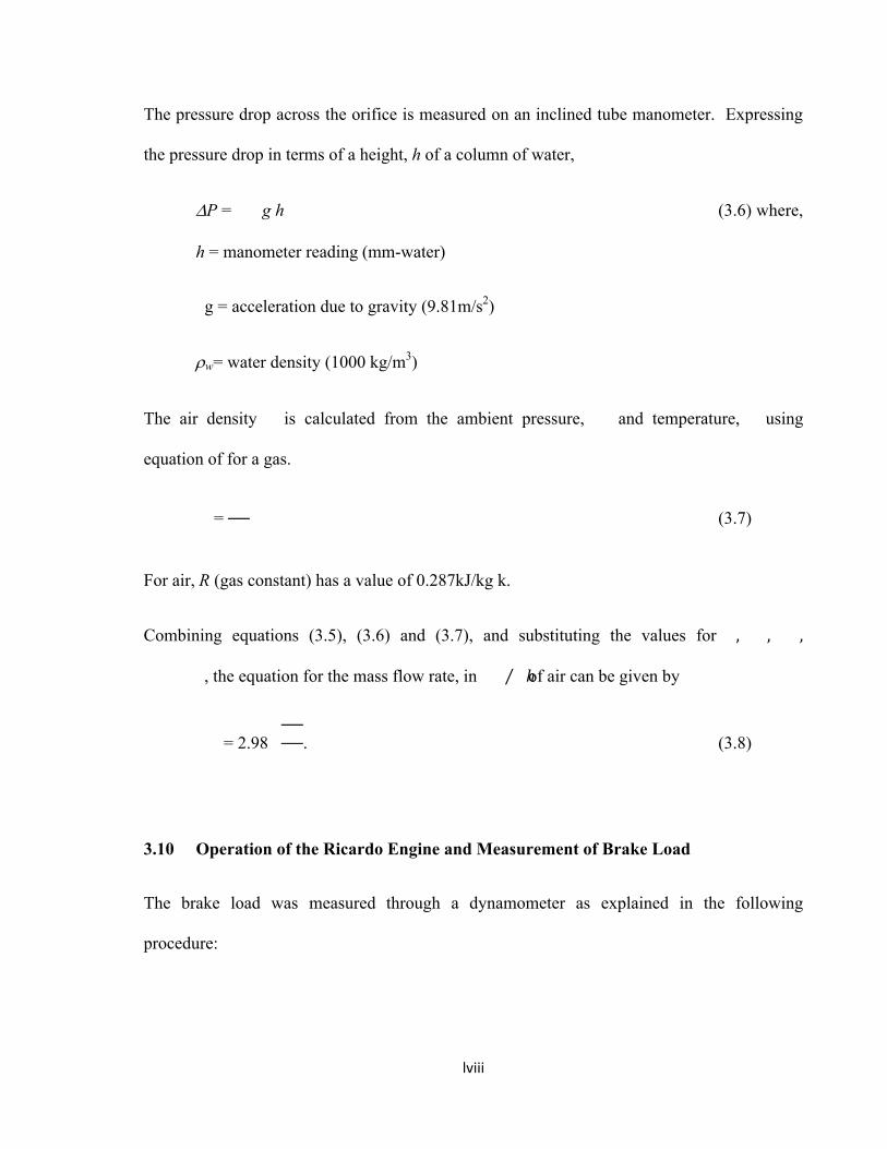
The pressure drop across the orifice is measured on an inclined tube manometer. Expressing
the pressure drop in terms of a height, h of a column of water,
P = g h (3.6) where,
h = manometer reading (mm-water)
g = acceleration due to gravity (9.81m/s2)
w= water density (1000 kg/m3)
The air density is calculated from the ambient pressure, and temperature, using
equation of for a gas.
= (3.7)
For air, R (gas constant) has a value of 0.287kJ/kg k.
Combining equations (3.5), (3.6) and (3.7), and substituting the values for , , , , the equation for the mass flow rate, in ℎ⁄ of air can be given by
= 2.98 . (3.8)
3.10 Operation of the Ricardo Engine and Measurement of Brake Load
The brake load was measured through a dynamometer as explained in the following
procedure:
lix
To kick-start the engine, the dynamometer motor was switched on by the switch gear. On
kick-starting, when the motor runs the engine to gain momentum, the ignition was switched
on and the engine ignited (fired). The motoring switch was turned on to the load (on the
panel). This made the engine to develop power. When the switch gear was released (off), the
motor became the load to the engine. The brake load was then measured and recorded with
respect to the compression ratio and engine speed.The torque arm was measured andthe time
taken for 50ml of the fuel to be consumed was taken and recorded.The brake torque was
calculated by the product of the torque arm and brake load. Then the brake power was
calculated by means of equation (2.2)
3.11 Theoretical Determination ofPerformance Characteristics
3.11.1 Calculation of torque gain/loss
Increase in compression ratio induces greater turning effect on the cylinder crank (Heywood,
1988). That means that the engine is getting more push on the piston, and hence more torque
is generated.The torque gain due to compression ratio increase can be given as the ratio of a
new compression ratio to the old compression ratio given by (PhilipandDavid,1954) as:
Torque gain = ( )0.4 (3.9)
In the cylinders the combustion process takes place, and converts the energy in the fuel to
power.Ideally, all the heat stored in the fuel may be converted to power; in that case the
delivered power is given by taking the product of the heating value of the fuel, and the
fuel mass flow rate, through the cylinders. However there will be losses during the energy
lx
conversion, thus we have to multiply with the brake thermal efficiency, (fuel conversion
efficiency) (Andreas, 2003)
= (3.10)
If equation (2.2) and (3.10) are equated, an equation for the relation between the engine torque
and mass flow rate of the fuel is developed as
T = / (3.11)
Where,N is the engine speed in rev/min
If the whole process is approximated to an Otto cycle(constant volume cycle), the conversion
efficiency can be calculated by (Andreas, 2003)
= k(1 - ) (3.12)
Kin equation (3.12) is a constant and it is introduced because in equation (1.1), energy losses
due to incomplete combustion, heat transfer from gas to cylinder walls and timing losses have
been neglected.Thus, equation (3.11) becomes
T = (1 - ) (3.13)
The values forK (from 1100 to 1600rpm in increments of 100rpm) were determined
experimentally for a reference compression ratio of 7by means of equation (3.13). (Values for
K are giving in Table 4.9). Compression ratio of 7 was used as the reference because it is mid-
way of the operational compression ratios. When a value greater than 7 was utilised (example,
9), the percentage error between the experimental and theoretical value was increases; but
with 7, the error reduces.
The theoretical torque gain from compression ratio of 7 to 8 and 7 to 9 were calculated by
means of equation (3.9), and the theoretical brake torque were obtained by adding the torque
lxi
gain to the experimental brake torque obtained at compression ratio of 7. Similar calculations
were carried out for the torque loss from compression ratio of 7 to 6 and 7 to 5 (appendix B).
With the theoretical brake torque, the theoretical mass flow rate of the fuel with respect to the
engine speeds, compression ratios and the K values, were calculated by
= (1- )-1 (3.14)
With the calculated torque and the K values from the reference compression ratio, the
theoretical mass flow rate of the fuel was calculated by means of equation (3.14). The
theoretical brake power, brake mean effective pressure, brake thermal efficiency and specific
fuel consumption were calculated by means of equations (2.2), (2.3), (2.5) and (2.7)
respectively.The results are giving in tables 4.4.1 to 4.4.10, and the calculations carried out in
Engineering Equation Solver (EES) computer programme are giving in appendix B.
3.11.2 Error analysis
The percentage error in the brake power, brake thermal efficiency, specific fuel consumption
and brake mean effective pressure were calculated by (Andreas, 2003).
Error =
x100% (3.15)
lxii
CHAPTER FOUR
RESULTS AND DISCUSSION
Equations used for calculating the derived values of brake power, indicated thermal
efficiency, specific fuel consumption and the brake mean effective pressure are as modelledin
appendix A and B using Engineering equation solver (EES) computer programme.
The Table of values for the experimental readings, calculated values from experimental
readings, improvement in the performance characteristics from the increase in compression
ratios, theoretical values and the error between the experimental and theoretical values are
giving in this section.
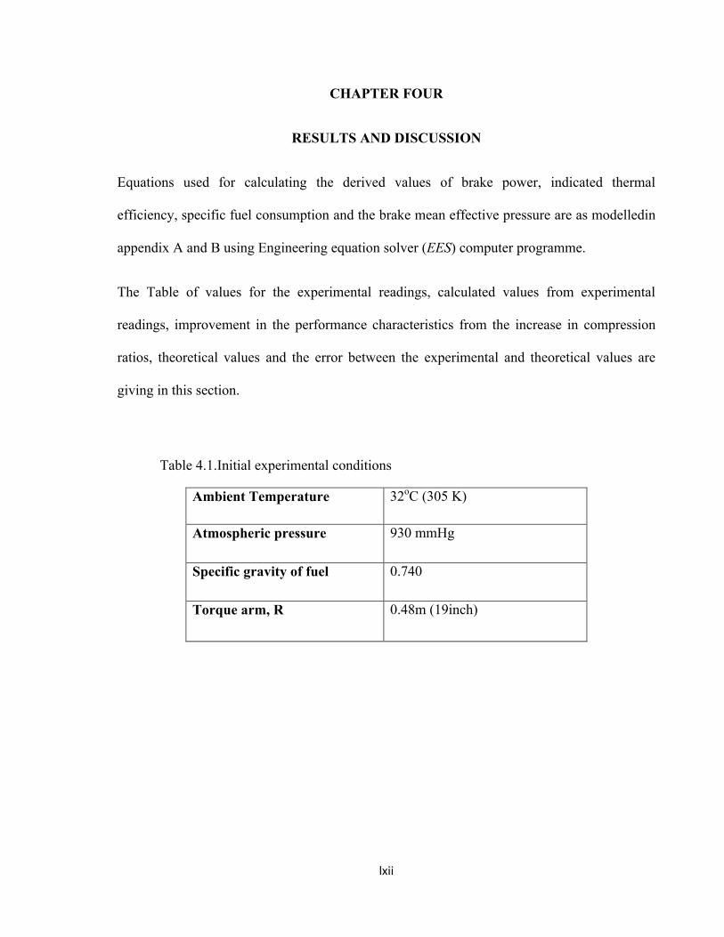
Table 4.1.Initial experimental conditions
Ambient Temperature 32oC (305 K)
Atmospheric pressure 930 mmHg
Specific gravity of fuel 0.740
Torque arm, R 0.48m (19inch)
lxiii
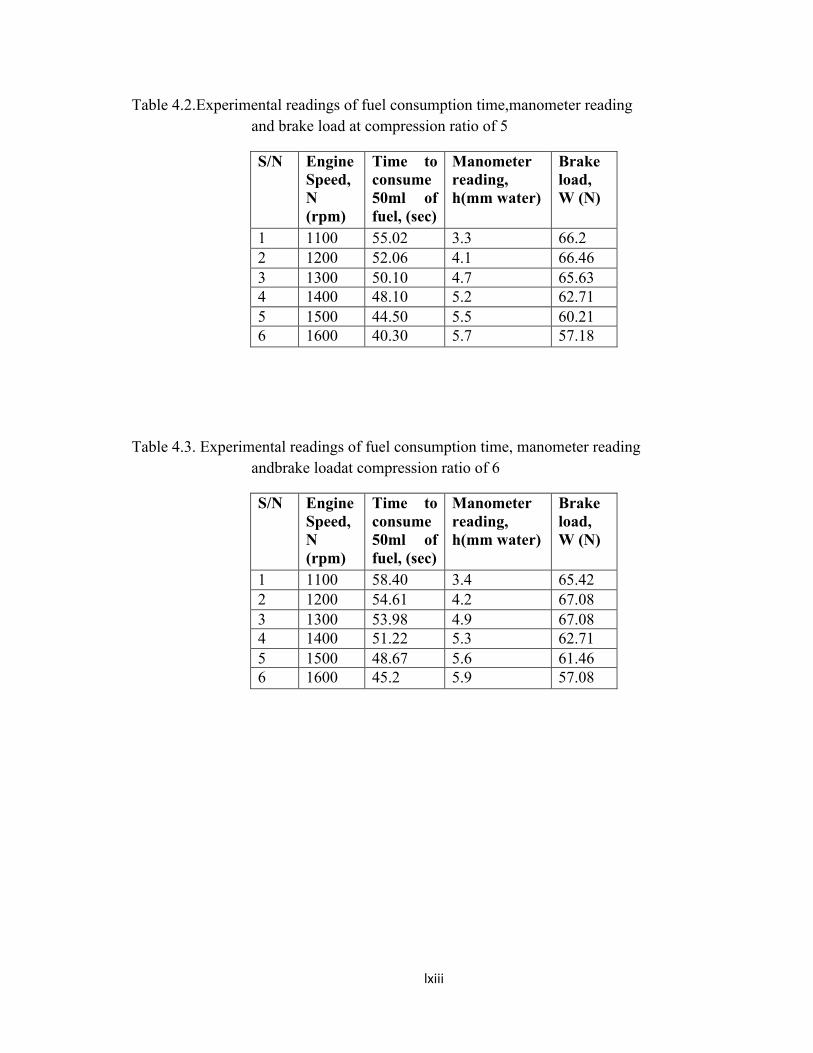
Table 4.2.Experimental readings of fuel consumption time,manometer reading and brake load at compression ratio of 5
Table 4.3. Experimental readings of fuel consumption time, manometer reading andbrake loadat compression ratio of 6
S/N Engine Speed, N (rpm)
Time to consume 50ml of fuel, (sec)
Manometer reading, h(mm water)
Brake load, W (N)
1 1100 58.40 3.4 65.422 1200 54.61 4.2 67.083 1300 53.98 4.9 67.084 1400 51.22 5.3 62.715 1500 48.67 5.6 61.466 1600 45.2 5.9 57.08
S/N Engine Speed, N (rpm)
Time to consume 50ml of fuel, (sec)
Manometer reading, h(mm water)
Brake load, W (N)
1 1100 55.02 3.3 66.22 1200 52.06 4.1 66.463 1300 50.10 4.7 65.634 1400 48.10 5.2 62.715 1500 44.50 5.5 60.216 1600 40.30 5.7 57.18
lxiv
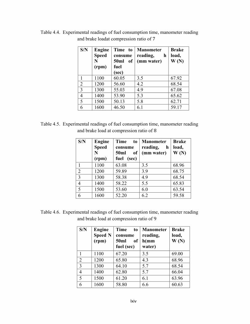
Table 4.4. Experimental readings of fuel consumption time, manometer reading and brake loadat compression ratio of 7
S/N Engine Speed N (rpm)
Time to consume 50ml of fuel (sec)
Manometer reading, h (mm water)
Brake load, W (N)
1 1100 60.05 3.5 67.922 1200 56.60 4.2 68.543 1300 55.03 4.9 67.084 1400 53.90 5.3 65.625 1500 50.13 5.8 62.716 1600 46.50 6.1 59.17
Table 4.5. Experimental readings of fuel consumption time, manometer reading and brake load at compression ratio of 8
Table 4.6. Experimental readings of fuel consumption time, manometer reading and brake load at compression ratio of 9
S/N Engine Speed N (rpm)
Time to consume 50ml of fuel (sec)
Manometer reading, h (mm water)
Brake load, W (N)
1 1100 63.08 3.5 68.962 1200 59.89 3.9 68.753 1300 58.38 4.9 68.544 1400 58.22 5.5 65.835 1500 53.60 6.0 63.546 1600 52.20 6.2 59.58
S/N Engine Speed N (rpm)
Time to consume 50ml of fuel (sec)
Manometer reading, h(mm water)
Brake load, W (N)
1 1100 67.20 3.5 69.002 1200 65.80 4.3 68.963 1300 64.10 5.7 68.544 1400 62.80 5.7 66.045 1500 61.20 6.1 63.966 1600 58.80 6.6 60.63
lxv
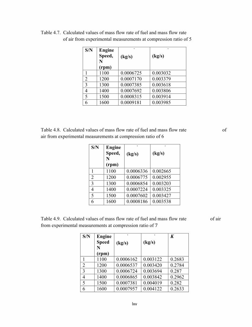
Table 4.7. Calculated values of mass flow rate of fuel and mass flow rate of air from experimental measurements at compression ratio of 5
Table 4.8. Calculated values of mass flow rate of fuel and mass flow rate of air from experimental measurements at compression ratio of 6
S/N Engine Speed, N (rpm)
(kg/s)
(kg/s)
1 1100 0.0006336 0.0026652 1200 0.0006775 0.0029553 1300 0.0006854 0.0032034 1400 0.0007224 0.0033255 1500 0.0007602 0.0034276 1600 0.0008186 0.003538
Table 4.9. Calculated values of mass flow rate of fuel and mass flow rate of air from experimental measurements at compression ratio of 7
S/N Engine Speed, N (rpm)
(kg/s)
(kg/s)
1 1100 0.0006725 0.0030322 1200 0.0007170 0.0033793 1300 0.0007385 0.0036184 1400 0.0007692 0.0038065 1500 0.0008315 0.0039146 1600 0.0009181 0.003985
S/N Engine Speed N (rpm)
(kg/s)
(kg/s)
K
1 1100 0.0006162 0.003122 0.26832 1200 0.0006537 0.003420 0.27843 1300 0.0006724 0.003694 0.2874 1400 0.0006865 0.003842 0.29625 1500 0.0007381 0.004019 0.2826 1600 0.0007957 0.004122 0.2633
lxvi
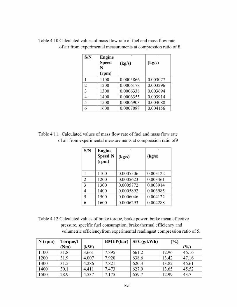
Table 4.10.Calculated values of mass flow rate of fuel and mass flow rate of air from experimental measurements at compression ratio of 8
Table 4.11. Calculated values of mass flow rate of fuel and mass flow rate of air from experimental measurements at compression ratio of9
Table 4.12.Calculated values of brake torque, brake power, brake mean effective pressure, specific fuel consumption, brake thermal efficiency and volumetric efficiencyfrom experimental readingsat compression ratio of 5.
N (rpm) Torque,T (Nm) (kW)
BMEP(bar) SFC(g/kWh) (%)(%)
1100 31.8 3.661 7.895 661.2 12.96 46.161200 31.9 4.007 7.920 638.6 13.42 47.161300 31.5 4.286 7.821 620.3 13.82 46.611400 30.1 4.411 7.473 627.9 13.65 45.521500 28.9 4.537 7.175 659.7 12.99 43.7
S/N Engine Speed N (rpm)
(kg/s)
(kg/s)
1 1100 0.0005866 0.0030772 1200 0.0006178 0.0032963 1300 0.0006338 0.0036944 1400 0.0006355 0.0039145 1500 0.0006903 0.0040886 1600 0.0007088 0.004156
S/N Engine Speed N (rpm)
(kg/s)
(kg/s)
1 1100 0.0005506 0.0031222 1200 0.0005623 0.0034613 1300 0.0005772 0.0039144 1400 0.0005892 0.0039855 1500 0.0006046 0.0041226 1600 0.0006293 0.004288
lxvii
1600 27.4 4.589 6.803 720.3 11.9 41.7
Table 4.13. Calculated values of brake torque, brake power, brake mean effective pressure, specific fuel consumption, brake thermal efficiency and volumetric efficiencyfrom experimental readings at compression ratio of6
N (rpm) Torque, T (Nm)
(kW) BMEP (bar)
SFC (g/kWh)
(%)(%)
1100 31.4 3.730 8.044 611.4 14.02 46.851200 32.2 4.044 7.994 603.1 14.21 47.731300 32.2 4.368 7.969 565.0 15.17 47.571400 30.1 4.543 7.696 572.5 14.97 45.961500 29.5 4.632 7.324 590.9 14.51 44.091600 27.9 4.672 6.927 630.7 13.59 42.43
Table 4.14.Calculated values of brake torque, brake power, brake mean effective pressure, specific fuel consumption, brake thermal efficiency and volumetric efficiencyfrom experimental readings at compression ratio of 7
N (rpm)
Torque, T (Nm) (kW)
BMEP(bar) SFC(g/kWh)(%) (%)
1100 32.6 3.753 8.094 591.0 14.50 47.53
1200 32.9 4.132 8.168 569.5 15.05 47.73
1300 32.2 4.381 7.994 552.5 15.52 47.591400 31.5 4.616 7.821 535.4 16.01 55.96
1500 30.1 4.726 7.473 562.3 15.24 44.87
1600 28.4 4.756 7.051 602.3 14.23 43.14
Table 4.15. Calculated values of brake torque, brake power, brake mean effective pressure, specific fuel consumption, brake thermal efficiency and volumetric efficiencyfrom experimental readings at compression ratio of 8
N (rpm)
Torque, T (Nm) (kW)
BMEP(bar) SFC (g/kWh) (%) (%)
1100 33.1 3.811 8.218 554.1 15.47 46.851200 33.0 4.145 8.193 536.1 15.97 46.001300 32.9 4.477 8.168 509.7 16.82 47.59
lxviii
1400 31.6 4.630 7.845 494.1 17.35 46.821500 30.5 4.789 7.572 519.0 16.52 45.641600 28.6 4.790 7.101 532.8 16.09 43.50
Table 4.16. Calculated values of brake torque, brake power, brake mean effective pressure, specific fuel consumption, brake thermal efficiency and volumetric efficiency from experimental readingsat compression ratio of 9.
N (rpm) Torque, T (Nm) (kW)
BMEP (bar)
SFC(g/kWh)(%) (%)
1100 33.3 4.834 8.267 517.0 16.58 47.531200 33.1 4.157 8.218 486.9 17.60 48.301300 32.9 4.477 8.168 464.2 18.47 50.421400 31.7 4.645 7.870 456.6 18.77 47.661500 30.7 4.820 7.622 451.6 18.98 46.021600 29.1 4.873 7.225 464.8 18.44 44.88
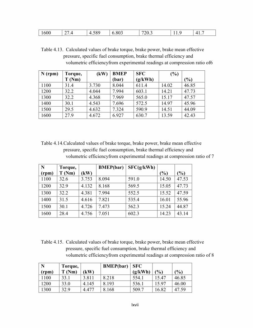
Figure 4.1. Variation of experimental brake power with compression ratio for different engine speeds.
5 5.5 6 6.5 7 7.5 8 8.5 9 9.5
2.8
3
3.2
3.4
3.6
3.8
4
4.2
4.4
4.6
4.8
5
5.2
Compression ratio
Brak
e Po
wer (
kW)
N =1100rpmN =1100rpmN =1200rpmN =1200rpmN =1300rpmN =1300rpm
N = 1400rpm N = 1400rpm
N =1500rpmN =1500rpmN =1600rpmN =1600rpm
lxix
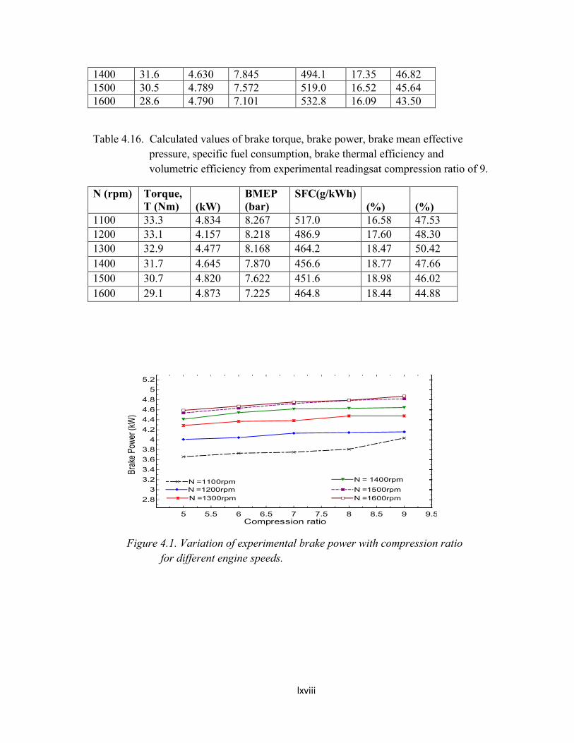
Figure 4.2.Variation of experimental brake power with engine speed for different compression ratios
Figure 4.3. Variation of experimental thermal efficiency with compression ratiofor different engine speeds.
1100 1200 1300 1400 1500 1600 1700
3.4
3.6
3.8
4
4.2
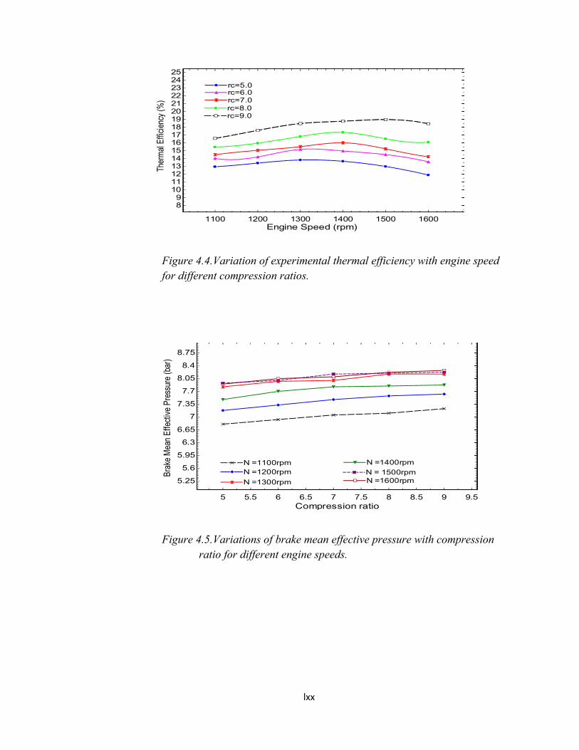
4.4
4.6
4.8
5
5.2
5.4
5.6
Engine Speed (rpm)
Brak
e Po
wer (
kW)
rc=5.0rc=5.0rc=6.0rc=6.0rc=7.0rc=7.0rc=8.0rc=8.0rc=9.0rc=9.0
4.5 5 5.5 6 6.5 7 7.5 8 8.5 9 9.5
10
11
12
13
14
15
16
17
18
19
20
21
Compression ratio
Ther
mal
Effi
cien
cy (%
)
N =1100rpmN =1100rpmN =1200rpmN =1200rpmN =1300rpmN =1300rpmN =1400rpmN =1400rpmN =1500rpmN =1500rpm
N =1600rpmN =1600rpm
lxx
Figure 4.4.Variation of experimental thermal efficiency with engine speed for different compression ratios.
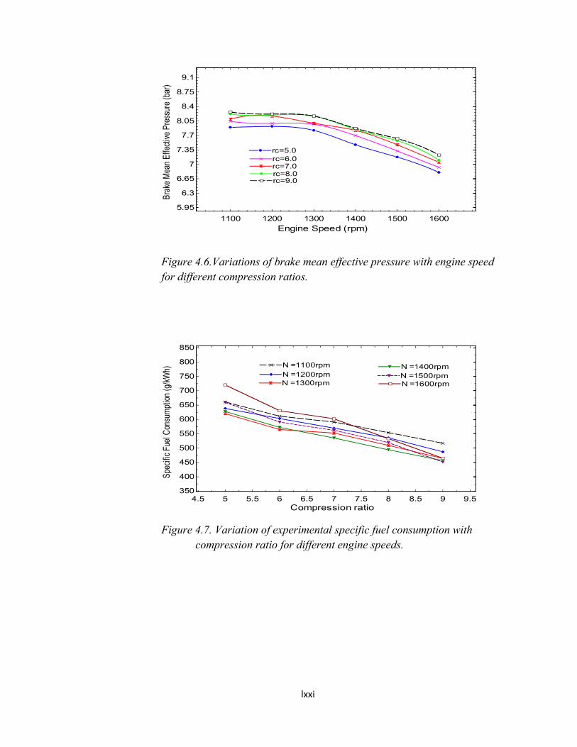
Figure 4.5.Variations of brake mean effective pressure with compression ratio for different engine speeds.
1100 1200 1300 1400 1500 1600
89
10111213141516171819202122232425
Engine Speed (rpm)
Ther
mal
Effi
cien
cy (%
)
rc=5.0rc=5.0rc=6.0rc=6.0rc=7.0rc=7.0rc=8.0rc=8.0rc=9.0rc=9.0
5 5.5 6 6.5 7 7.5 8 8.5 9 9.5
5.25
5.6
5.95
6.3
6.65
7
7.35
7.7
8.05
8.4
8.75
Compression ratio
Brak
e M
ean
Effe
ctiv
e Pr
essu
re (b
ar)
N =1600rpmN =1600rpmN = 1500rpmN = 1500rpm
N =1300rpmN =1300rpm
N =1400rpmN =1400rpmN =1200rpmN =1200rpmN =1100rpmN =1100rpm
lxxi
Figure 4.6.Variations of brake mean effective pressure with engine speed for different compression ratios.
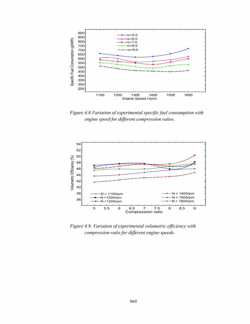
Figure 4.7. Variation of experimental specific fuel consumption with compression ratio for different engine speeds.
1100 1200 1300 1400 1500 1600
5.95
6.3
6.65
7
7.35
7.7
8.05
8.4
8.75
9.1
Engine Speed (rpm)
Brak
e M
ean
Effe
ctiv
e Pr
essu
re (b
ar)
rc=5.0rc=5.0rc=6.0rc=6.0rc=7.0rc=7.0rc=8.0rc=8.0rc=9.0rc=9.0
4.5 5 5.5 6 6.5 7 7.5 8 8.5 9 9.5350
400
450
500
550
600
650
700
750
800
850
Compression ratio
Spec
ific
Fuel
Con
sum
ptio
n (g
/kW
h) N =1100rpmN =1100rpmN =1200rpmN =1200rpmN =1300rpmN =1300rpm
N =1400rpmN =1400rpmN =1500rpmN =1500rpmN =1600rpmN =1600rpm
lxxii
Figure 4.8.Variation of experimental specific fuel consumption with engine speed for different compression ratios.
Figure 4.9. Variation of experimental volumetric efficiency with compression ratio for different engine speeds.
1100 1200 1300 1400 1500 1600
250
300350400450500
550600650
700750800
850900
Engine Speed (rpm)
Spec
ific
Fuel
Con
sum
ptio
n (g
/kW
h)
rc=5.0rc=5.0rc=6.0rc=6.0rc=7.0rc=7.0rc=8.0rc=8.0rc=9.0rc=9.0
5 5.5 6 6.5 7 7.5 8 8.5 9
36
38
40
42
44
46
48
50
52
54
Compression ratio
Volu
met
ric E
ffici
ency
(%)
N = 1100rpmN = 1100rpmN =1200rpmN =1200rpmN =1300rpmN =1300rpm
N = 1400rpmN = 1400rpmN = 1500rpmN = 1500rpmN = 1600rpmN = 1600rpm
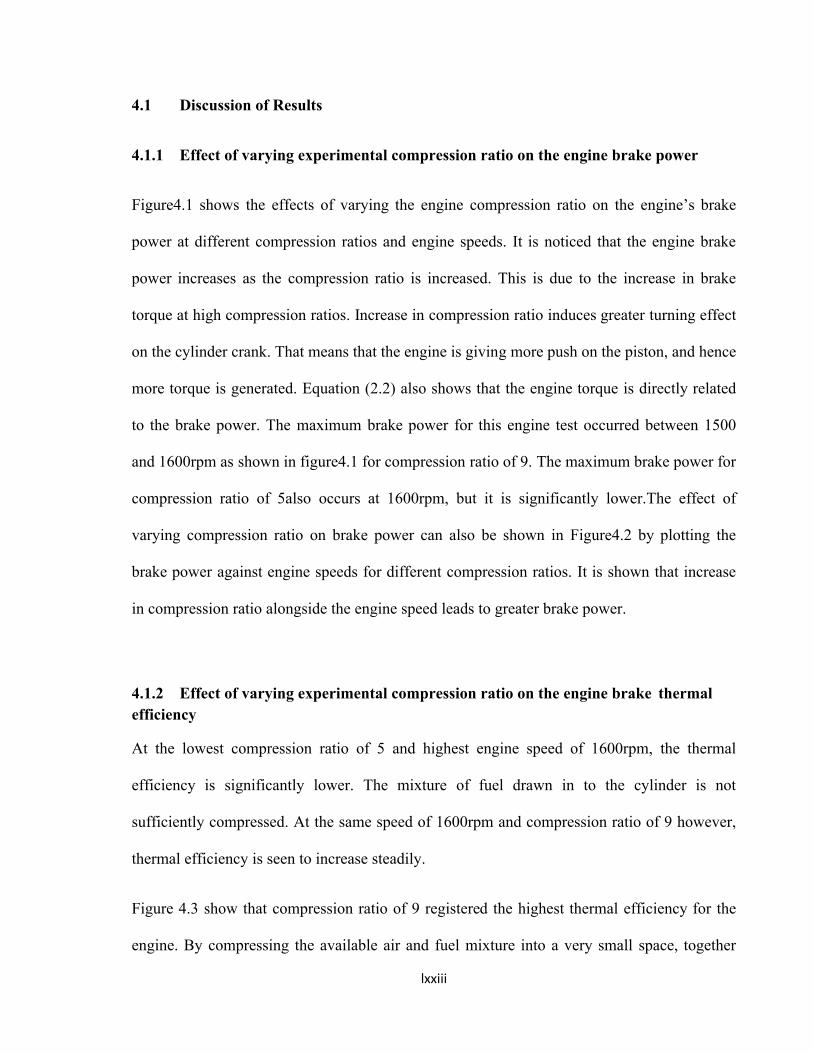
lxxiii
4.1 Discussion of Results
4.1.1 Effect of varying experimental compression ratio on the engine brake power
Figure4.1 shows the effects of varying the engine compression ratio on the engine’s brake
power at different compression ratios and engine speeds. It is noticed that the engine brake
power increases as the compression ratio is increased. This is due to the increase in brake
torque at high compression ratios. Increase in compression ratio induces greater turning effect
on the cylinder crank. That means that the engine is giving more push on the piston, and hence
more torque is generated. Equation (2.2) also shows that the engine torque is directly related
to the brake power. The maximum brake power for this engine test occurred between 1500
and 1600rpm as shown in figure4.1 for compression ratio of 9. The maximum brake power for
compression ratio of 5also occurs at 1600rpm, but it is significantly lower.The effect of
varying compression ratio on brake power can also be shown in Figure4.2 by plotting the
brake power against engine speeds for different compression ratios. It is shown that increase
in compression ratio alongside the engine speed leads to greater brake power.
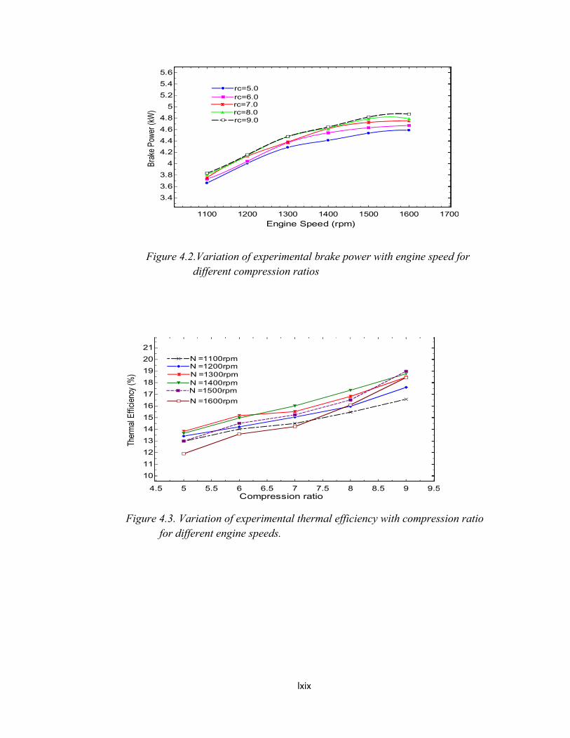
4.1.2 Effect of varying experimental compression ratio on the engine brake thermal efficiency
At the lowest compression ratio of 5 and highest engine speed of 1600rpm, the thermal
efficiency is significantly lower. The mixture of fuel drawn in to the cylinder is not
sufficiently compressed. At the same speed of 1600rpm and compression ratio of 9 however,
thermal efficiency is seen to increase steadily.
Figure 4.3 show that compression ratio of 9 registered the highest thermal efficiency for the
engine. By compressing the available air and fuel mixture into a very small space, together
lxxiv
with the heat of compression, causes better mixing and evaporation of the fuel. Greater
combustion efficiency from increasing compression ratio means that the combustion of the
fuel pays greater dividends by more energy released from the fuel. The net result is that the
increase in energy available is greater. The highest thermal efficiency, according to figure 4.3
occurredat 1500rpm and compression ratio of 9
4.1.3 Effect of varying experimental compression ratio on brake mean effective pressure
Increase in the brake mean effective pressure in the cylinder(from high temperature and
pressure of the working fluid at the end of combustion), is developed by increased in the
compression ratiosas shown in figure 4.5. The figure also shows that the mean effective
pressure reduces with engine speed. Equation 2.3 also agrees with this. As the compression
ratio increases, the cylinder is subjected to higher temperatures, leading to higher brake mean
effective pressures. Equation 2.4 also shows that brake mean effective pressure is directly
proportional to the torque. From figure 4.5, compression ratios of 8 and 9 developed the
highest brake mean effective pressure. A plot of the brake mean effective pressure against
speed for the various compression ratios is shown in figure 4.6; similar resultsare obtained
showing that increasing the compression ratio from 5 to 8 and 9, increases the brake mean
effective pressure.
4.1.4 Effect of varying experimental compression ratio on fuel consumption parameters
lxxv
The effects of varying the compression ratios on the engine’s fuel consumption parameters are
shown in figure 4.7. Figure 4.7 can be understood with the help of the result in Figure 4.3 and
4.4. From equation (2.8), the specific fuel consumption is inversely proportional to the
thermal efficiency. As the compression ratio increases, the fuel mixture is sufficiently
compressed thereby increasing the thermal efficiency, so that less fuel is used to produce the
same amount of energy. Fuel consumption per kilowatts of time is reduced at higher
compression ratios between 8 and 9. With the increase in compression ratios,a higher engine
speed of 1600rpm favours the reduction in fuel consumption as shown in Figure4.7. Figure
4.8 further shows the variation of the specific fuel consumption with engine speed for
different compression ratios. In the figure, it is clearly shown that the highest compression
ratio of 9gave the lowest specific fuel consumption; whereas at compression ratio of 5, the
specific fuel consumption recorded the highest value.
4.1.5 Effect of varying experimental compression ratio on volumetric efficiency
In general, the volumetric efficiency increases very slowly with increase compression
ratio.However, Figure 4.9 shows that beyond compression ratio of 8, the volumetric efficiency
increases rapidly. By increasing the compression ratio, the clearance volume reduces;
therebyreducing the denominator of equation(2.12). At compression ratio of 9 and at low
engine speeds of 1200 and 1300 rpm, the volumetric efficiency is relatively higher compared
to high engine speeds of 1500 and 1600 rpm. This is because the engine speed is inversely
proportional to the volumetric efficiency (equation 2.12).
4.2 Improvement in the Engine Performance Characteristics from Increase in the Compression Ratio
lxxvi
Improvement in the engine performance characteristics from increase in the compression ratio
from 5 to 6, 6 to 7, 7 to 8 and 8 to 9 were calculated and tabulated.
Table 4.17.Improvement in brake power
N (rpm)
(%) Increase in (kW)=5 =6 =7 =8 =9 from
=5 to
=6
from =6
to=7
from =7
to=8
from =8
to=9
Average (%)
1100 3.661 3.730 3.753 3.811 3.834 1.88 0.62 1.55 0.60 1.161200 4.007 4.044 4.132 4.145 4.157 0.92 2.18 0.31 0.29 0.931300 4.286 4.368 4.381 4.477 4.417 1.91 0.29 2.91 1.34 1.611400 4.411 4.543 4.616 4.630 4.645 2.99 1.61 0.30 0.32 1.311500 4.537 4.632 4.726 4.789 4.820 2.09 2.03 1.33 0.65 1.531600 4.589 4.672 4.756 4.790 4.873 1.81 1.80 0.71 1.73 1.51
Grand average =
1.34
Table 4.18.Improvement in brake thermal efficiency
N (rpm)
(%) Increase in
=5 =6 =7 =8 =9 from =5
to=6
from =6
to=7
from =7
to=8
from=8
to=9
Average (%)
1100 12.96 14.02 14.50 15.47 16.58 8.18 3.42 6.69 7.18 6.371200 13.42 14.21 15.05 15.97 17.6 5.81 5.91 6.11 10.21 7.011300 13.82 15.17 15.52 16.82 18.47 9.77 2.31 8.38 9.81 7.571400 13.65 14.97 16.01 17.35 18.77 9.67 7.23 8.37 8.18 8.341500 12.99 14.51 15.24 16.52 18.98 11.7 5.03 8.40 14.89 10.011600 11.9 13.59 14.23 16.09 18.44 14.2 4.71 13.07 14.61 11.65
Grand average =
8.49
Table 4.19.Reduction in specific fuel consumption
lxxvii
N (rpm)
(%) Increase in SFC (g/kW h)=5 =6 =7 =8 =9 from
=5 to
=6
from =6
to=7
from =7
to=8
from =8
to=9
Average (%)
1100 661.2 611.0 591.0 555.1 517.0 7.53 3.34 6.66 6.70 6.061200 638.6 603.1 569.5 536.1 486.9 5.56 5.57 5.86 9.18 6.541300 620.3 565.0 552.5 509.7 464.2 8.92 2.21 7.75 8.93 6.951400 627.9 572.5 535.4 494.1 456.6 8.82 6.48 7.71 7.59 7.651500 659.7 590.9 562.3 519.0 451.6 10.43 4.84 7.70 12.99 8.991600 720.3 630.7 602.3 532.8 464.8 12.44 4.50 11.54 12.76 10.31
Grand average =
7.75
Table 4.20.Improvement in brake mean effective pressure
N
(rpm)(%) Increase in BMEP(bar)
=5 =6 =7 =8 =9 from
=5 to
=6
from
=6 to
=7
from
=7 to
=8
from
=8to
=9
Average (%)
1100
7.89500
8.04396
8.09362
8.21775
8.26740
1.89 0.62 1.53 0.60 1.16
1200
7.91983
7.99431
8.16810
8.19292
8.21775
0.93 2.17 0.30 0.30 0.93
1300
7.82052
7.96948
7.99431
8.11810
8.16810
1.89 0.31 2.17 0.62 1.25
1400
7.47294
7.69638
7.82052
7.84534
7.87017
2.98 1.63 0.32 0.32 1.31
1500
7.17501
7.32398
7.47294
7.57225
7.62190
2.08 2.03 1.33 0.66 1.53
1600
6.80261
6.92674
7.05088
7.10053
7.22467
1.82 1.79 0.74 1.75 1.53
Grand average =
1.29
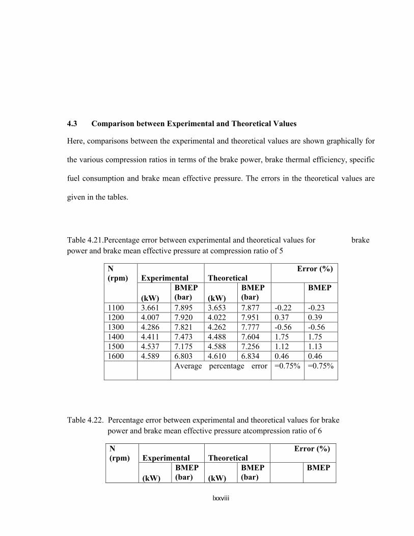
lxxviii
4.3 Comparison between Experimental and Theoretical Values
Here, comparisons between the experimental and theoretical values are shown graphically for
the various compression ratios in terms of the brake power, brake thermal efficiency, specific
fuel consumption and brake mean effective pressure. The errors in the theoretical values are
given in the tables.
Table 4.21.Percentage error between experimental and theoretical values for brake power and brake mean effective pressure at compression ratio of 5
N (rpm)
Experimental
Theoretical
Error (%)
(kW)BMEP (bar) (kW)
BMEP (bar)
BMEP
1100 3.661 7.895 3.653 7.877 -0.22 -0.231200 4.007 7.920 4.022 7.951 0.37 0.391300 4.286 7.821 4.262 7.777 -0.56 -0.561400 4.411 7.473 4.488 7.604 1.75 1.751500 4.537 7.175 4.588 7.256 1.12 1.131600 4.589 6.803 4.610 6.834 0.46 0.46
Average percentage error =0.75% =0.75%
Table 4.22. Percentage error between experimental and theoretical values for brake power and brake mean effective pressure atcompression ratio of 6
N (rpm)
Experimental
Theoretical
Error (%)
(kW)BMEP (bar) (kW)
BMEP (bar)
BMEP
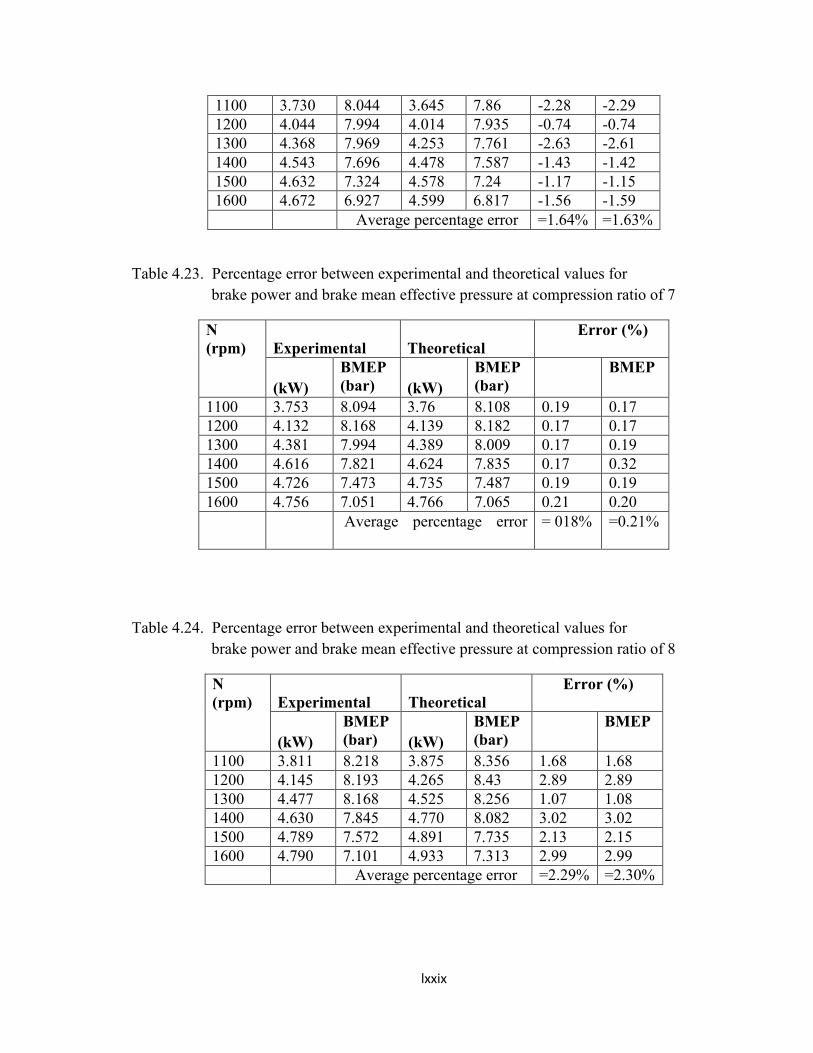
lxxix
1100 3.730 8.044 3.645 7.86 -2.28 -2.291200 4.044 7.994 4.014 7.935 -0.74 -0.741300 4.368 7.969 4.253 7.761 -2.63 -2.611400 4.543 7.696 4.478 7.587 -1.43 -1.421500 4.632 7.324 4.578 7.24 -1.17 -1.151600 4.672 6.927 4.599 6.817 -1.56 -1.59
Average percentage error =1.64% =1.63%
Table 4.23. Percentage error between experimental and theoretical values for brake power and brake mean effective pressure at compression ratio of 7
N (rpm)
Experimental
Theoretical
Error (%)
(kW)BMEP (bar) (kW)
BMEP (bar)
BMEP
1100 3.753 8.094 3.76 8.108 0.19 0.171200 4.132 8.168 4.139 8.182 0.17 0.171300 4.381 7.994 4.389 8.009 0.17 0.191400 4.616 7.821 4.624 7.835 0.17 0.321500 4.726 7.473 4.735 7.487 0.19 0.191600 4.756 7.051 4.766 7.065 0.21 0.20
Average percentage error = 018% =0.21%
Table 4.24. Percentage error between experimental and theoretical values for brake power and brake mean effective pressure at compression ratio of 8
N (rpm)
Experimental
Theoretical
Error (%)
(kW)BMEP (bar) (kW)
BMEP (bar)
BMEP
1100 3.811 8.218 3.875 8.356 1.68 1.681200 4.145 8.193 4.265 8.43 2.89 2.891300 4.477 8.168 4.525 8.256 1.07 1.081400 4.630 7.845 4.770 8.082 3.02 3.021500 4.789 7.572 4.891 7.735 2.13 2.151600 4.790 7.101 4.933 7.313 2.99 2.99
Average percentage error =2.29% =2.30%
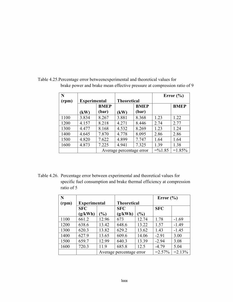
lxxx
Table 4.25.Percentage error betweenexperimental and theoretical values for brake power and brake mean effective pressure at compression ratio of 9
N (rpm)
Experimental
Theoretical
Error (%)
(kW)BMEP (bar) (kW)
BMEP (bar)
BMEP
1100 3.834 8.267 3.881 8.368 1.23 1.221200 4.157 8.218 4.271 8.446 2.74 2.771300 4.477 8.168 4.532 8.269 1.23 1.241400 4.645 7.870 4.778 8.095 2.86 2.861500 4.820 7.622 4.899 7.747 1.64 1.641600 4.873 7.225 4.941 7.325 1.39 1.38
Average percentage error =%1.85 =1.85%
Table 4.26. Percentage error between experimental and theoretical values for specific fuel consumption and brake thermal efficiency at compression
ratio of 5
N (rpm)
Experimental
Theoretical
Error (%)
SFC (g/kWh) (%)
SFC (g/kWh) (%)
SFC
1100 661.2 12.96 673 12.74 1.78 -1.691200 638.6 13.42 648.6 13.22 1.57 -1.491300 620.3 13.82 629.2 13.62 1.43 -1.451400 627.9 13.65 609.6 14.06 -2.91 3.001500 659.7 12.99 640.3 13.39 -2.94 3.081600 720.3 11.9 685.8 12.5 -4.79 5.04
Average percentage error =2.57% =2.13%
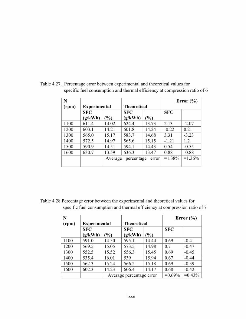
lxxxi
Table 4.27. Percentage error between experimental and theoretical values for specific fuel consumption and thermal efficiency at compression ratio of 6
N(rpm)
Experimental
Theoretical
Error (%)
SFC (g/kWh) (%)
SFC (g/kWh) (%)
SFC
1100 611.4 14.02 624.4 13.73 2.13 -2.071200 603.1 14.21 601.8 14.24 -0.22 0.211300 565.0 15.17 583.7 14.68 3.31 -3.231400 572.5 14.97 565.6 15.15 -1.21 1.21500 590.9 14.51 594.1 14.43 0.54 -0.551600 630.7 13.59 636.3 13.47 0.88 -0.88
Average percentage error =1.38% =1.36%
Table 4.28.Percentage error between the experimental and theoretical values for specific fuel consumption and thermal efficiency at compression ratio of 7
N (rpm)
Experimental
Theoretical
Error (%)
SFC (g/kWh) (%)
SFC (g/kWh) (%)
SFC
1100 591.0 14.50 595.1 14.44 0.69 -0.411200 569.5 15.05 573.5 14.98 0.7 -0.471300 552.5 15.52 556.3 15.45 0.69 -0.451400 535.4 16.01 539 15.94 0.67 -0.441500 562.3 15.24 566.2 15.18 0.69 -0.391600 602.3 14.23 606.4 14.17 0.68 -0.42
Average percentage error =0.69% =0.43%
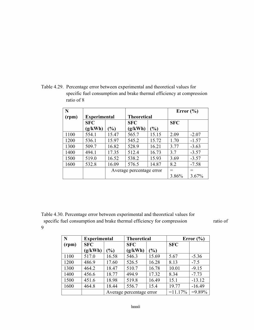
lxxxii
Table 4.29. Percentage error between experimental and theoretical values for specific fuel consumption and brake thermal efficiency at compression
ratio of 8
N (rpm)
Experimental
Theoretical
Error (%)
SFC (g/kWh) (%)
SFC (g/kWh) (%)
SFC
1100 554.1 15.47 565.7 15.15 2.09 -2.071200 536.1 15.97 545.2 15.72 1.70 -1.571300 509.7 16.82 528.9 16.21 3.77 -3.631400 494.1 17.35 512.4 16.73 3.7 -3.571500 519.0 16.52 538.2 15.93 3.69 -3.571600 532.8 16.09 576.5 14.87 8.2 -7.58
Average percentage error = 3.86%
= 3.67%
Table 4.30. Percentage error between experimental and theoretical values for specific fuel consumption and brake thermal efficiency for compression ratio of 9
N (rpm)
Experimental Theoretical Error (%)SFC (g/kWh) (%)
SFC (g/kWh) (%)
SFC
1100 517.0 16.58 546.3 15.69 5.67 -5.361200 486.9 17.60 526.5 16.28 8.13 -7.51300 464.2 18.47 510.7 16.78 10.01 -9.151400 456.6 18.77 494.9 17.32 8.34 -7.731500 451.6 18.98 519.8 16.49 15.1 -13.121600 464.8 18.44 556.7 15.4 19.77 -16.49
Average percentage error =11.17% =9.89%
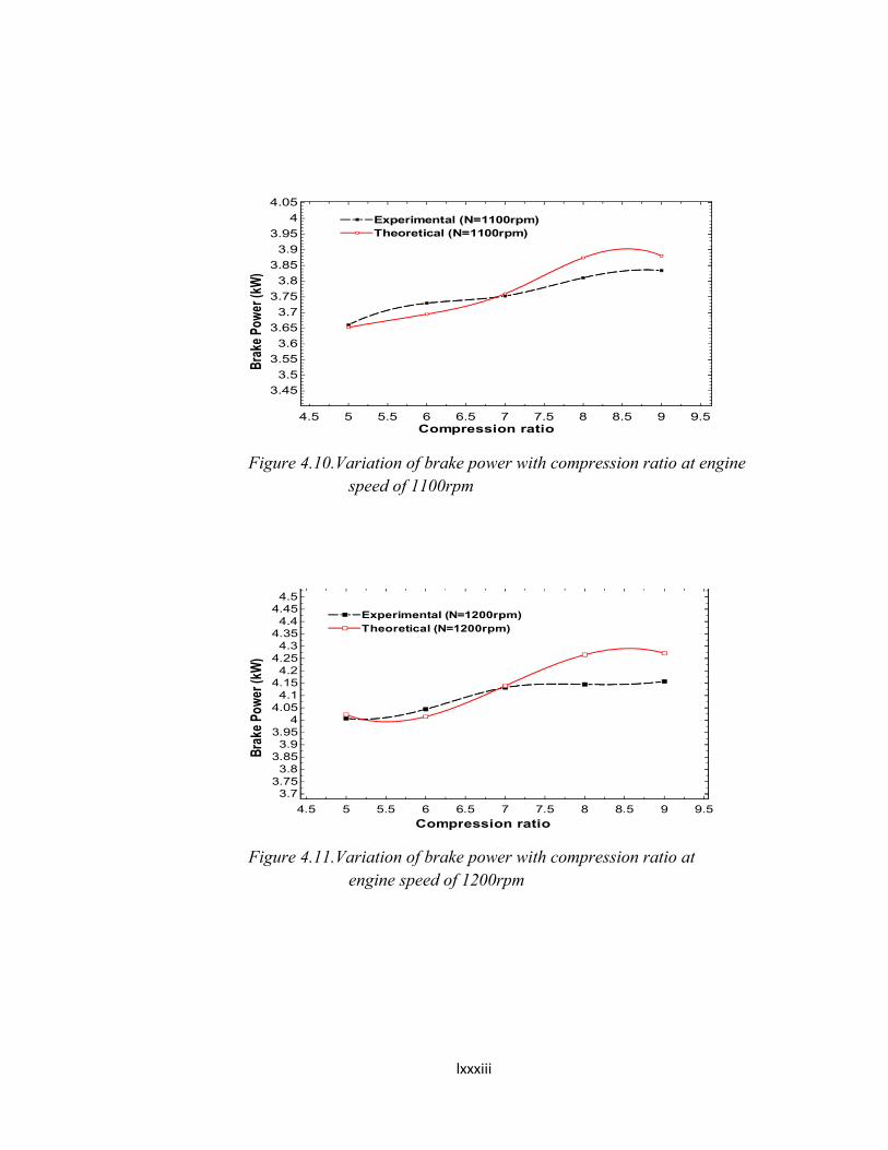
lxxxiii
Figure 4.10.Variation of brake power with compression ratio at engine speed of 1100rpm
Figure 4.11.Variation of brake power with compression ratio at engine speed of 1200rpm
4.5 5 5.5 6 6.5 7 7.5 8 8.5 9 9.5
3.45
3.5
3.55
3.6
3.65
3.7
3.75
3.8
3.85
3.9
3.95
4
4.05
Compression ratio
Brak
ePo
wer
(kW
)
Experimental (N=1100rpm)Experimental (N=1100rpm)Theoretical (N=1100rpm)Theoretical (N=1100rpm)
4.5 5 5.5 6 6.5 7 7.5 8 8.5 9 9.5
3.73.753.8
3.853.9
3.954
4.054.1
4.154.2
4.254.3
4.354.4
4.454.5
Compression ratio
Brak
ePo
wer
(kW
)
Experimental (N=1200rpm)Experimental (N=1200rpm)Theoretical (N=1200rpm)Theoretical (N=1200rpm)
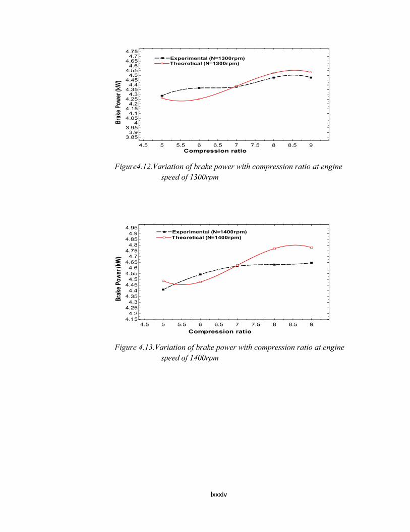
lxxxiv
Figure4.12.Variation of brake power with compression ratio at engine speed of 1300rpm
Figure 4.13.Variation of brake power with compression ratio at engine speed of 1400rpm
4.5 5 5.5 6 6.5 7 7.5 8 8.5 9
3.853.9
3.954
4.054.1
4.154.2
4.254.3
4.354.4
4.454.5
4.554.6
4.654.7
4.75
Compression ratio
Brak
ePo
wer
(kW
)
Experimental (N=1300rpm)Experimental (N=1300rpm)Theoretical (N=1300rpm)Theoretical (N=1300rpm)
4.5 5 5.5 6 6.5 7 7.5 8 8.5 94.154.2
4.254.3
4.354.4
4.454.5
4.554.6
4.654.7
4.754.8
4.854.9
4.95
Compression ratio
Brak
ePo
wer
(kW
)
Experimental (N=1400rpm)Experimental (N=1400rpm)Theoretical (N=1400rpm)Theoretical (N=1400rpm)
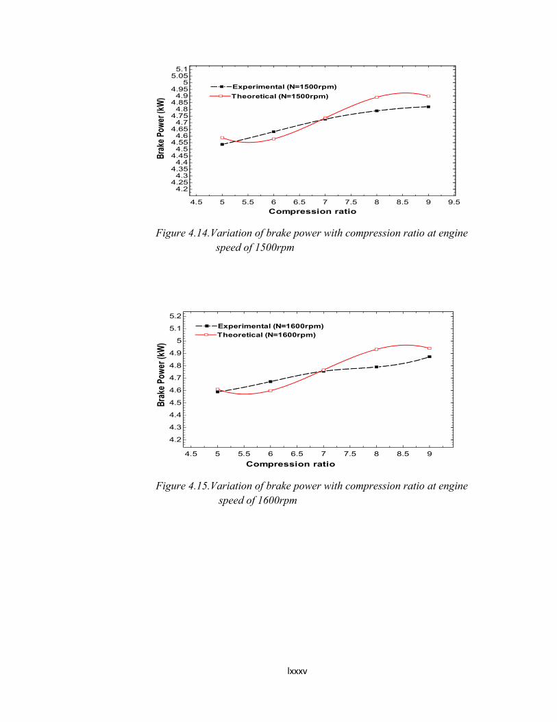
lxxxv
Figure 4.14.Variation of brake power with compression ratio at engine speed of 1500rpm
Figure 4.15.Variation of brake power with compression ratio at engine speed of 1600rpm
4.5 5 5.5 6 6.5 7 7.5 8 8.5 9 9.5
4.24.254.3
4.354.4
4.454.5
4.554.6
4.654.7
4.754.8
4.854.9
4.955
5.055.1
Compression ratio
Brak
ePo
wer
(kW
)
Experimental (N=1500rpm)Experimental (N=1500rpm)
Theoretical (N=1500rpm)Theoretical (N=1500rpm)
4.5 5 5.5 6 6.5 7 7.5 8 8.5 9
4.2
4.3
4.4
4.5
4.6
4.7
4.8
4.9
5
5.1
5.2
Compression ratio
Brak
ePo
wer
(kW
)
Experimental (N=1600rpm)Experimental (N=1600rpm)Theoretical (N=1600rpm)Theoretical (N=1600rpm)
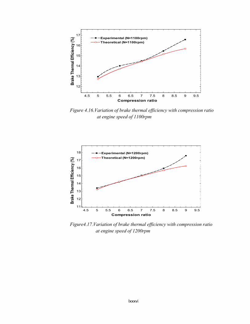
lxxxvi
Figure 4.16.Variation of brake thermal efficiency with compression ratio at engine speed of 1100rpm
Figure4.17.Variation of brake thermal efficiency with compression ratio at engine speed of 1200rpm
4.5 5 5.5 6 6.5 7 7.5 8 8.5 9 9.5
12
13
14
15
16
17
Compression ratio
Bra
keTh
erm
alEf
ficie
ncy
(%) Experimental (N=1100rpm)Experimental (N=1100rpm)
Theoretical (N=1100rpm)Theoretical (N=1100rpm)
4.5 5 5.5 6 6.5 7 7.5 8 8.5 9 9.511
12
13
14
15
16
17
18
Compression ratio
Brak
eTh
erm
alEf
ficie
ncy
(%)
Experimental (N=1200rpm)Experimental (N=1200rpm)
Theoretical (N=1200rpm)Theoretical (N=1200rpm)
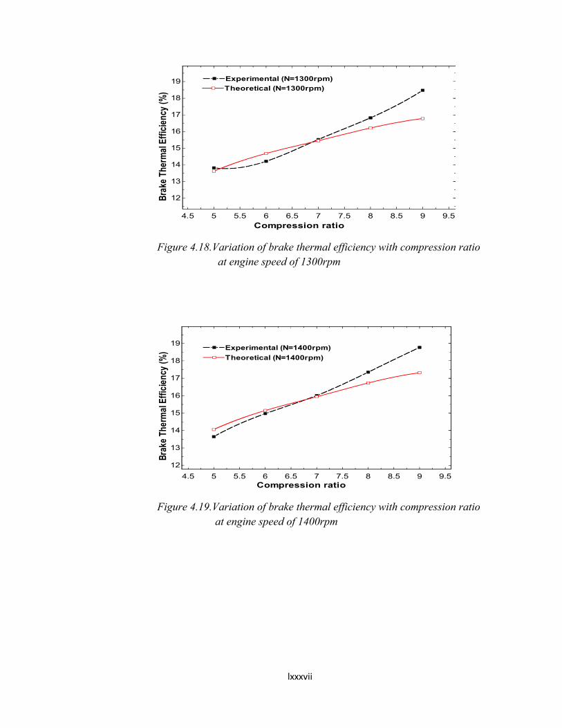
lxxxvii
Figure 4.18.Variation of brake thermal efficiency with compression ratio at engine speed of 1300rpm
Figure 4.19.Variation of brake thermal efficiency with compression ratio at engine speed of 1400rpm
4.5 5 5.5 6 6.5 7 7.5 8 8.5 9 9.5
12
13
14
15
16
17
18
19
Compression ratio
Brak
eTh
erm
alEf
ficie
ncy
(%)
Experimental (N=1300rpm)Experimental (N=1300rpm)
Theoretical (N=1300rpm)Theoretical (N=1300rpm)
4.5 5 5.5 6 6.5 7 7.5 8 8.5 9 9.5
12
13
14
15
16
17
18
19
Compression ratio
Brak
eTh
erm
alEf
ficie
ncy
(%) Experimental (N=1400rpm)Experimental (N=1400rpm)
Theoretical (N=1400rpm)Theoretical (N=1400rpm)
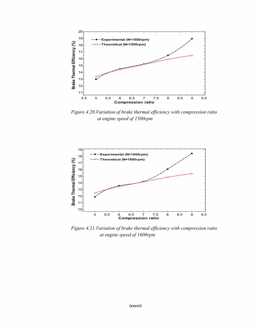
lxxxviii
Figure 4.20.Variation of brake thermal efficiency with compression ratio at engine speed of 1500rpm
Figure 4.21.Variation of brake thermal efficiency with compression ratio at engine speed of 1600rpm
4.5 5 5.5 6 6.5 7 7.5 8 8.5 9 9.5
11
12
13
14
15
16
17
18
19
20
Compression ratio
Brak
eTh
erm
alEf
ficie
ncy
(%) Experimental (N=1500rpm)Experimental (N=1500rpm)
Theoretical (N=1500rpm)Theoretical (N=1500rpm)
5 5.5 6 6.5 7 7.5 8 8.5 9 9.5
10
11
12
13
14
15
16
17
18
19
Compression ratio
Brak
eTh
erm
alEf
ficie
ncy
(%)
Experimental (N=1600rpm)Experimental (N=1600rpm)
Theoretical (N=1600rpm)Theoretical (N=1600rpm)
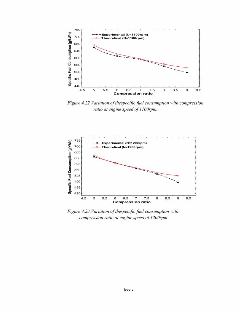
lxxxix
Figure 4.22.Variation of thespecific fuel consumption with compression ratio at engine speed of 1100rpm.
Figure 4.23.Variation of thespecific fuel consumption with compression ratio at engine speed of 1200rpm.
4.5 5 5.5 6 6.5 7 7.5 8 8.5 9 9.5
440
480
520
560
600
640
680
720
760
Compression ratio
Spec
ific
Fuel
Cons
umpt
ion
(g/k
Wh) Experimental (N=1100rpm)Experimental (N=1100rpm)
Theoretical (N=1100rpm)Theoretical (N=1100rpm)
4.5 5 5.5 6 6.5 7 7.5 8 8.5 9 9.5
420
455
490
525
560
595
630
665
700
735
Compression ratio
Spec
ific
Fuel
Cons
umpt
ion
(g/k
Wh) Experimental (N=1200rpm)Experimental (N=1200rpm)
Theoretical (N=1200rpm)Theoretical (N=1200rpm)
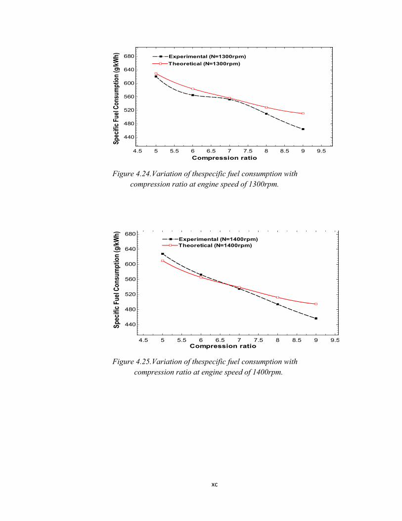
xc
Figure 4.24.Variation of thespecific fuel consumption with compression ratio at engine speed of 1300rpm.
Figure 4.25.Variation of thespecific fuel consumption with compression ratio at engine speed of 1400rpm.
4.5 5 5.5 6 6.5 7 7.5 8 8.5 9 9.5
440
480
520
560
600
640
680
Compression ratio
Spec
ific
Fuel
Cons
umpt
ion
(g/k
Wh) Experimental (N=1300rpm)Experimental (N=1300rpm)
Theoretical (N=1300rpm)Theoretical (N=1300rpm)
4.5 5 5.5 6 6.5 7 7.5 8 8.5 9 9.5
440
480
520
560
600
640
680
Compression ratio
Spec
ific
Fuel
Cons
umpt
ion
(g/k
Wh)
Experimental (N=1400rpm)Experimental (N=1400rpm)Theoretical (N=1400rpm)Theoretical (N=1400rpm)
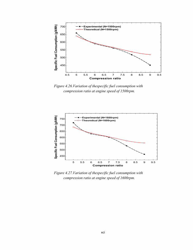
xci
Figure 4.26.Variation of thespecific fuel consumption with compression ratio at engine speed of 1500rpm.
Figure 4.27.Variation of thespecific fuel consumption with compression ratio at engine speed of 1600rpm.
4.5 5 5.5 6 6.5 7 7.5 8 8.5 9 9.5
450
500
550
600
650
700
Compression ratio
Spec
ific
Fuel
Cons
umpt
ion
(g/k
Wh) Experimental (N=1500rpm)Experimental (N=1500rpm)
Theoretical (N=1500rpm)Theoretical (N=1500rpm)
5 5.5 6 6.5 7 7.5 8 8.5 9 9.5
450
500
550
600
650
700
750
Compression ratio
Spec
ific
Fuel
Cons
umpt
ion
(g/k
Wh) Experimental (N=1600rpm)Experimental (N=1600rpm)
Theoretical (N=1600rpm)Theoretical (N=1600rpm)

xcii
Figure 4.28.Variation of brake mean effective pressure with compression ratio at engine speed of 1100rpm.
Figure 4.29.Variation of brake mean effective pressure with compression ratio at engine speed of 1200rpm.
4.5 5 5.5 6 6.5 7 7.5 8 8.5 9 9.56.9
77.17.27.37.47.57.67.77.87.9
88.18.28.38.48.58.68.78.88.9
9
Compression ratio
Brak
eM
ean
Effe
ctiv
ePr
essu
re(b
ar)
Experimental (1100rpm)Experimental (1100rpm)
Theoretical (1100rpm)Theoretical (1100rpm)
5 5.5 6 6.5 7 7.5 8 8.5 9 9.5
7.17.27.37.47.57.67.77.87.9
88.18.28.38.48.58.68.78.88.9
99.1
Compression ratio
Brak
eM
ean
Effe
ctiv
ePr
essu
re(b
ar)
Experimental (N=1200rpm)Experimental (N=1200rpm)
Theoretical (N=1200rpm)Theoretical (N=1200rpm)
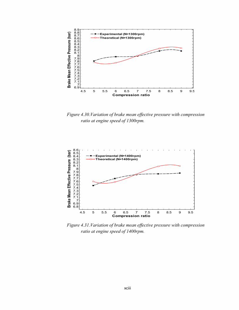
xciii
Figure 4.30.Variation of brake mean effective pressure with compression ratio at engine speed of 1300rpm.
Figure 4.31.Variation of brake mean effective pressure with compression ratio at engine speed of 1400rpm.
4.5 5 5.5 6 6.5 7 7.5 8 8.5 9 9.56.9
77.17.27.37.47.57.67.77.87.9
88.18.28.38.48.58.68.78.88.9
Compression ratio
Brak
eM
ean
Effe
ctiv
ePr
essu
re(b
ar)
Experimental (N=1300rpm)Experimental (N=1300rpm)Theoretical (N=1300rpm)Theoretical (N=1300rpm)
4.5 5 5.5 6 6.5 7 7.5 8 8.5 9 9.5
6.86.9
77.17.27.37.47.57.67.77.87.9
88.18.28.38.48.58.6
Compression ratio
Brak
eM
ean
Effe
ctiv
ePr
essu
re(b
ar)
Experimental (N=1400rpm)Experimental (N=1400rpm)Theoretical (N=1400rpm)Theoretical (N=1400rpm)
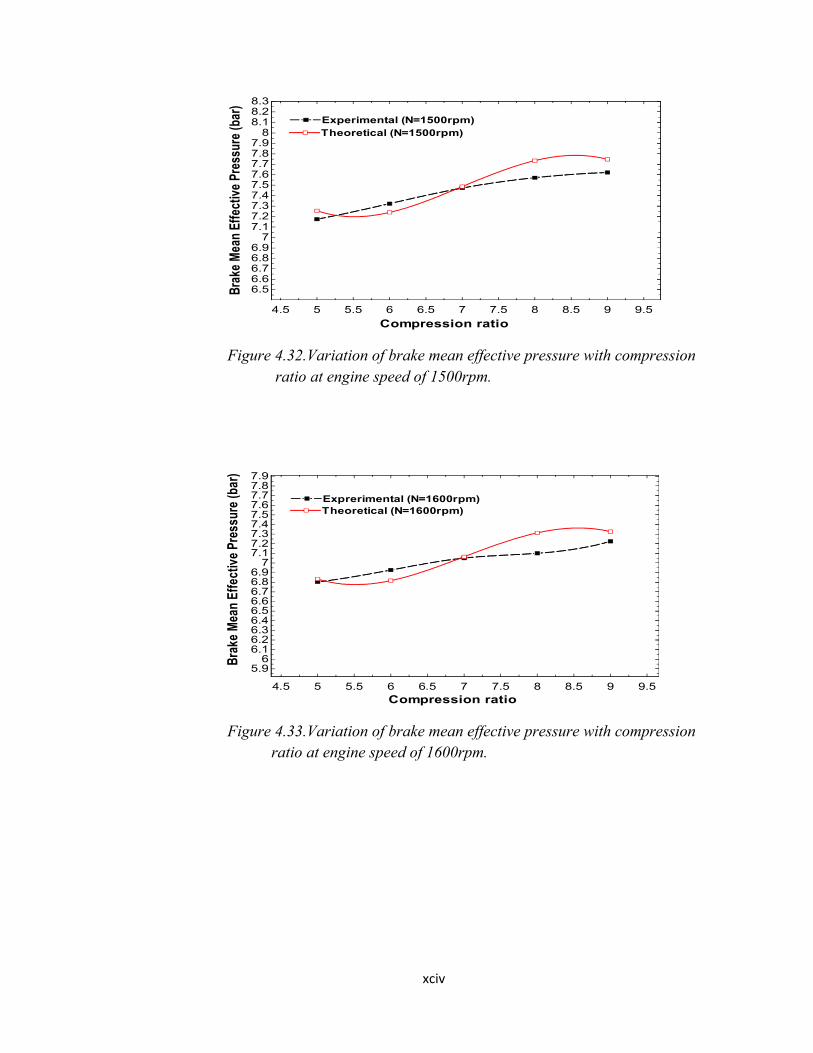
xciv
Figure 4.32.Variation of brake mean effective pressure with compression ratio at engine speed of 1500rpm.
Figure 4.33.Variation of brake mean effective pressure with compression ratio at engine speed of 1600rpm.
4.5 5 5.5 6 6.5 7 7.5 8 8.5 9 9.5
6.56.66.76.86.9
77.17.27.37.47.57.67.77.87.9
88.18.28.3
Compression ratio
Brak
eM
ean
Effe
ctiv
ePr
essu
re(b
ar)
Experimental (N=1500rpm)Experimental (N=1500rpm)Theoretical (N=1500rpm)Theoretical (N=1500rpm)
4.5 5 5.5 6 6.5 7 7.5 8 8.5 9 9.5
5.96
6.16.26.36.46.56.66.76.86.9
77.17.27.37.47.57.67.77.87.9
Compression ratio
Brak
eM
ean
Effe
ctiv
ePr
essu
re(b
ar)
Exprerimental (N=1600rpm)Exprerimental (N=1600rpm)Theoretical (N=1600rpm)Theoretical (N=1600rpm)
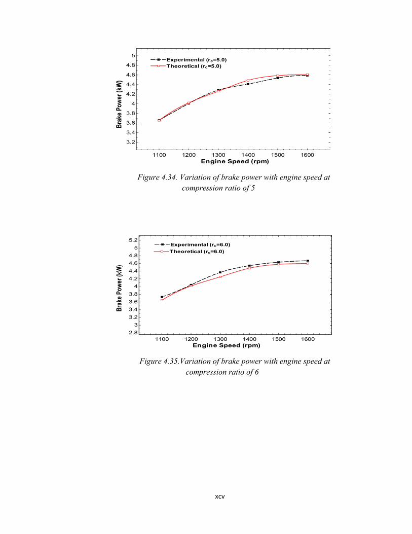
xcv
Figure 4.34. Variation of brake power with engine speed at compression ratio of 5
Figure 4.35.Variation of brake power with engine speed at compression ratio of 6
1100 1200 1300 1400 1500 1600
3.2
3.4
3.6
3.8
4
4.2
4.4
4.6
4.8
5
Engine Speed (rpm)
Brak
ePo
wer
(kW
)
Experimental (rc=5.0)Experimental (rc=5.0)Theoretical (rc=5.0)Theoretical (rc=5.0)
1100 1200 1300 1400 1500 16002.8
3
3.2
3.4
3.6
3.8
4
4.2
4.4
4.6
4.8
5
5.2
Engine Speed (rpm)
Brak
ePo
wer
(kW
)
Experimental (rc=6.0)Experimental (rc=6.0)
Theoretical (rc=6.0)Theoretical (rc=6.0)
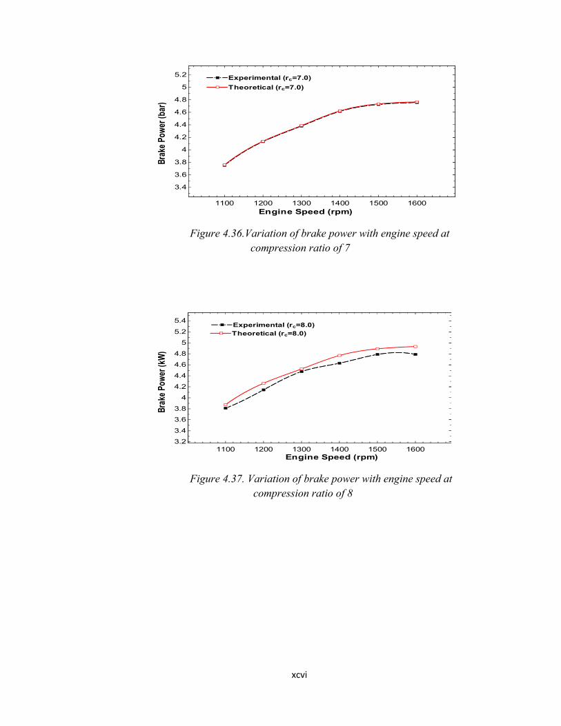
xcvi
Figure 4.36.Variation of brake power with engine speed at compression ratio of 7
Figure 4.37. Variation of brake power with engine speed at compression ratio of 8
1100 1200 1300 1400 1500 1600
3.4
3.6
3.8
4
4.2
4.4
4.6
4.8
5
5.2
Engine Speed (rpm)
Brak
ePo
wer
(bar
)
Experimental (rc=7.0)Experimental (rc=7.0)
Theoretical (rc=7.0)Theoretical (rc=7.0)
1100 1200 1300 1400 1500 16003.2
3.4
3.6
3.8
4
4.2
4.4
4.6
4.8
5
5.2
5.4
Engine Speed (rpm)
Brak
ePo
wer
(kW
)
Experimental (rc=8.0)Experimental (rc=8.0)Theoretical (rc=8.0)Theoretical (rc=8.0)
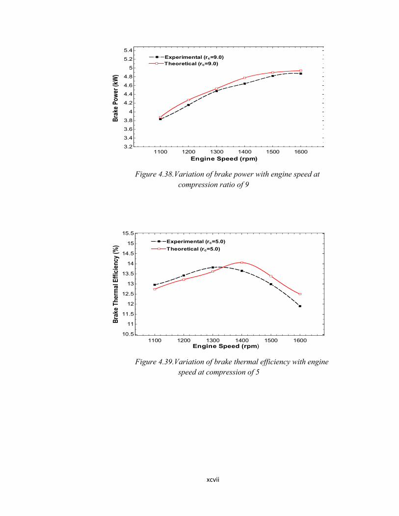
xcvii
Figure 4.38.Variation of brake power with engine speed at compression ratio of 9
Figure 4.39.Variation of brake thermal efficiency with engine speed at compression of 5
1100 1200 1300 1400 1500 16003.2
3.4
3.6
3.8
4
4.2
4.4
4.6
4.8
5
5.2
5.4
Engine Speed (rpm)
Bra
kePo
wer
(kW
)
Experimental (rc=9.0)Experimental (rc=9.0)Theoretical (rc=9.0)Theoretical (rc=9.0)
1100 1200 1300 1400 1500 160010.5
11
11.5
12
12.5
13
13.5
14
14.5
15
15.5
Engine Speed (rpm)
Bra
keTh
erm
alEf
ficie
ncy
(%)
Experimental (rc=5.0)Experimental (rc=5.0)
Theoretical (rc=5.0)Theoretical (rc=5.0)
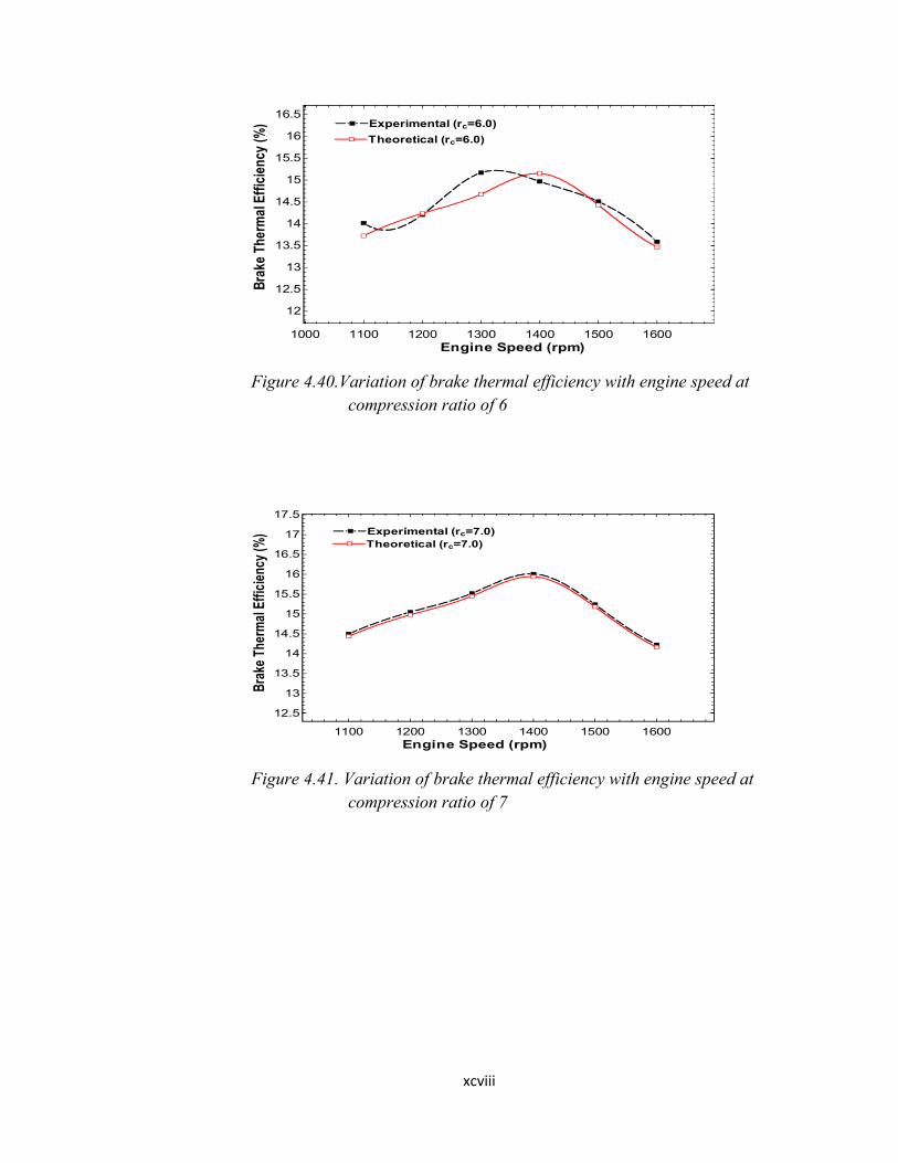
xcviii
Figure 4.40.Variation of brake thermal efficiency with engine speed at compression ratio of 6
Figure 4.41. Variation of brake thermal efficiency with engine speed at compression ratio of 7
1000 1100 1200 1300 1400 1500 1600
12
12.5
13
13.5
14
14.5
15
15.5
16
16.5
Engine Speed (rpm)
Brak
eTh
erm
alEf
ficie
ncy
(%) Experimental (rc=6.0)Experimental (rc=6.0)
Theoretical (rc=6.0)Theoretical (rc=6.0)
1100 1200 1300 1400 1500 1600
12.5
13
13.5
14
14.5
15
15.5
16
16.5
17
17.5
Engine Speed (rpm)
Brak
eTh
erm
alEf
ficie
ncy
(%) Experimental (rc=7.0)Experimental (rc=7.0)
Theoretical (rc=7.0)Theoretical (rc=7.0)
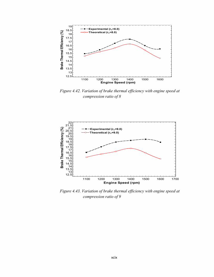
xcix
Figure 4.42. Variation of brake thermal efficiency with engine speed at compression ratio of 8
Figure 4.43. Variation of brake thermal efficiency with engine speed at compression ratio of 9
1100 1200 1300 1400 1500 160012.5
13
13.5
14
14.5
15
15.5
16
16.5
17
17.5
18
18.5
19
Engine Speed (rpm)
Brak
eTh
erm
alEf
ficie
ncy
(%) Experimental (rc=8.0)Experimental (rc=8.0)
Theoretical (rc=8.0)Theoretical (rc=8.0)
1100 1200 1300 1400 1500 1600 1700
12.513
13.514
14.515
15.516
16.517
17.518
18.519
19.520
20.521
21.522
Engine Speed (rpm)
Bra
keTh
erm
alEf
ficie
ncy
(%)
Experimental (rc=9.0)Experimental (rc=9.0)Theoretical (rc=9.0)Theoretical (rc=9.0)
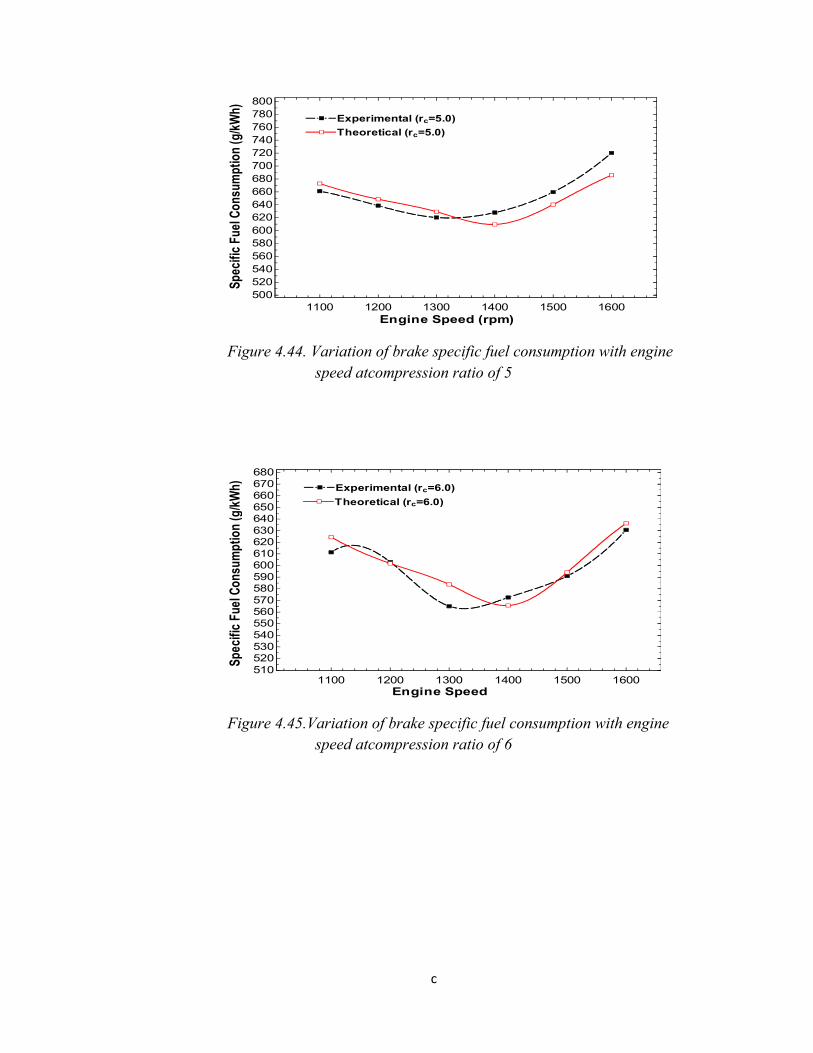
c
Figure 4.44. Variation of brake specific fuel consumption with engine speed atcompression ratio of 5
Figure 4.45.Variation of brake specific fuel consumption with engine speed atcompression ratio of 6
1100 1200 1300 1400 1500 1600500520540560580600620640660680700720740760780800
Engine Speed (rpm)
Spec
ific
Fuel
Cons
umpt
ion
(g/k
Wh)
Experimental (rc=5.0)Experimental (rc=5.0)
Theoretical (rc=5.0)Theoretical (rc=5.0)
1100 1200 1300 1400 1500 1600510520530540550560570580590600610620630640650660670680
Engine Speed
Spec
ific
Fuel
Cons
umpt
ion
(g/k
Wh) Experimental (rc=6.0)Experimental (rc=6.0)
Theoretical (rc=6.0)Theoretical (rc=6.0)
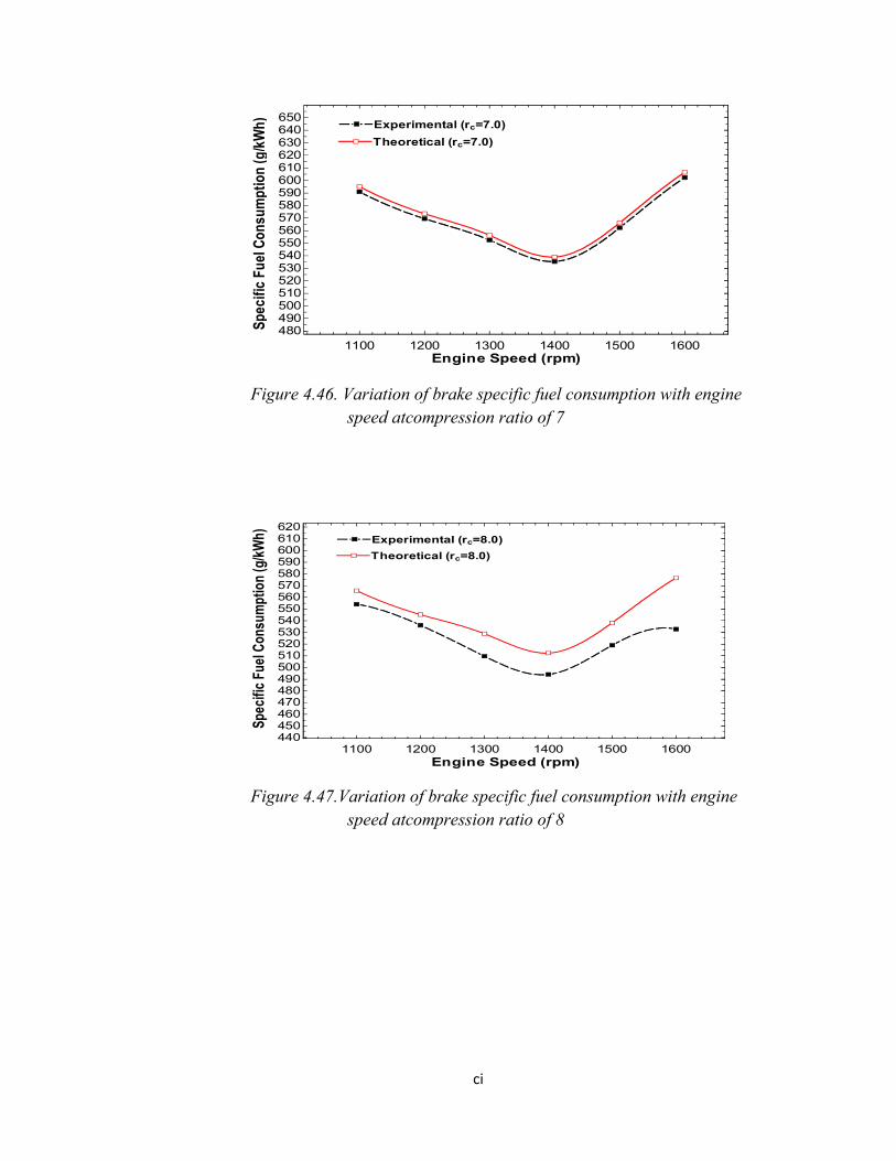
ci
Figure 4.46. Variation of brake specific fuel consumption with engine speed atcompression ratio of 7
Figure 4.47.Variation of brake specific fuel consumption with engine speed atcompression ratio of 8
1100 1200 1300 1400 1500 1600480490500510520530540550560570580590600610620630640650
Engine Speed (rpm)
Spec
ific
Fuel
Con
sum
ptio
n(g
/kW
h) Experimental (rc=7.0)Experimental (rc=7.0)
Theoretical (rc=7.0)Theoretical (rc=7.0)
1100 1200 1300 1400 1500 1600440450460470480490500510520530540550560570580590600610620
Engine Speed (rpm)
Spec
ific
Fuel
Cons
umpt
ion
(g/k
Wh) Experimental (rc=8.0)Experimental (rc=8.0)
Theoretical (rc=8.0)Theoretical (rc=8.0)
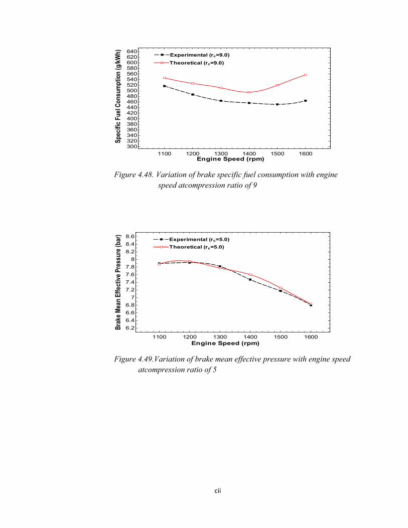
cii
Figure 4.48. Variation of brake specific fuel consumption with engine speed atcompression ratio of 9
Figure 4.49.Variation of brake mean effective pressure with engine speed atcompression ratio of 5
1100 1200 1300 1400 1500 1600
300320340360380400420440460480500520540560580600620640
Engine Speed (rpm)
Spec
ific
Fuel
Cons
umpt
ion
(g/k
Wh) Experimental (rc=9.0)Experimental (rc=9.0)
Theoretical (rc=9.0)Theoretical (rc=9.0)
1100 1200 1300 1400 1500 1600
6.2
6.4
6.6
6.8
7
7.2
7.4
7.6
7.8
8
8.2
8.4
8.6
Engine Speed (rpm)
Brak
eM
ean
Effe
ctiv
ePr
essu
re(b
ar)
Experimental (rc=5.0)Experimental (rc=5.0)
Theoretical (rc=5.0)Theoretical (rc=5.0)
ciii
Figure 4.50.Variation of brake mean effective pressure with engine speed atcompression ratio of 6
Figure 4.51.Variation of brake mean effective pressure with engine speed atcompression ratio of 7
1000 1100 1200 1300 1400 1500 1600
6.3
6.65
7
7.35
7.7
8.05
8.4
8.75
Engine Speed (rpm)
Brak
eM
ean
Effe
ctiv
ePr
essu
re(b
ar)
Experimental (rc=6.0)Experimental (rc=6.0)
Theoretical (rc=6.0)Theoretical (rc=6.0)
1100 1200 1300 1400 1500 1600
6.6
6.8
7
7.2
7.4
7.6
7.8
8
8.2
8.4
8.6
8.8
Engine Speed (rpm)
Brak
eM
ean
Effe
ctiv
ePr
essu
re(b
ar)
Experimental (rc=7.0)Experimental (rc=7.0)
Theoretical (rc=7.0)Theoretical (rc=7.0)
civ
Figure 4.52.Variation of brake mean effective pressure with engine speed atcompression ratio of 8
Figure 4.53.Variation of brake mean effective pressure with engine speed at compression ratio of 9
1000 1100 1200 1300 1400 1500 1600
6.8
7
7.2
7.4
7.6
7.8
8
8.2
8.4
8.6
8.8
9
9.2
Engine Speed (rpm)
Brak
eM
ean
Effe
ctiv
ePr
eesu
re(b
ar)
Experimental (rc=8.0)Experimental (rc=8.0)
Theoretical (rc=8.0)Theoretical (rc=8.0)
1100 1200 1300 1400 1500 1600
7
7.2
7.4
7.6
7.8
8
8.2
8.4
8.6
8.8
9
Engine Speed (rpm)
Brak
eM
ean
Effe
ctiv
ePr
essu
re(b
ar)
Experimental (rc=9.0)Experimental (rc=9.0)Theoretical (rc=9.0)Theoretical (rc=9.0)
cv
4.4 Comparison between Experimental and Theoretical Performance
Characteristics
4.4.1Brake power–Figures 4.10 to 4.15 shows the relation of the brake power with
compression ratio for both experimental and theoretical values. At low compression ratios of
5 and 6, theoretical values are lower than experimental values.As the compression ratio
increases to 8 and 9, the theoretical brake power increases beyond the experimental values.
This is because actual efficiency, and hence the brake power, is substantially below theoretical
efficiency. Compression and expansion of gases is not adiabatic, there are friction losses in
the engine. Complete combustion does not occur and work is required to draw in and exhaust
gases.
Figures 4.34 to 4.38 also show the variation of brake power with engine speed at various
compression ratios. At low compression ratios ( =5, =6), theoretical values are marginally
lower than experimental values. It also appears that as the speed increases with compression
ratio, the theoretical values increase more than the experimental values. It would then appears
that equation 3.9 overestimates the torque gainfor >6.
At compression ratio of 7, the theoretical and experimental values are almost equal. This is
because the values of K used in the theoretical analysis were obtained experimentally with
reference compression ratio of 7.
Tables 4.21 to 4.25, gives the percentage error between the experimental and theoretical
values. From the tables, the percentage error in the brake power tends to increase with
increase in compression ratio. At compression ratio of 7 (the reference compression ratio), the
minimum percentage error of 0.18% was obtained.
cvi
4.4.2Brake thermal efficiency–Figures 4.16 to 4.21shows the variation of the brake thermal
efficiency with compression ratio at various engine speeds. As the compression ratio increases
from 5 to 8, theoretical brake thermal efficiency is higher than experimental at 5 and 6, but
decreases at 8 and 9.In Figures 4.39 to 4.43 also, it appears that as the compression ratio
increases, the theoretical thermal efficiency decreases below the experimental value. It means
that the theoretical thermal efficiency was underestimated for compression ratio beyond 7.
From Tables 4.26 to 4.30, it is shown thatthe percentage error in the brake thermal efficiency
also tends to increase with increase in the compression ratio. At =5, the percentage error is
2.13%, while at =8 and 9, the percentage error is 3.67% and 9.89% respectively. The
minimum error of 0.43% occurred at =7.
4.4.3Specific fuel consumption - In Figures 4.22 to 4.27, the theoretical specific fuel
consumption shows similar trend with that of the experimentalvalues. Theoretical specific fuel
consumption is higher than the experimental at all points of the compression ratios. This is
due to the lower values of the theoretical brake thermal efficiency which makes the fuel
consumption to rise theoretically. Equation 2.9 also supports this; specific fuel consumption is
inversely proportional to thermal efficiency. In Figures 4.44 to 4.48 also, the general trend is
that the calculated theoretical specific fuel consumption is higher than the experimental value.
Tables 4.26 to 4.30 showsthat the percentage error in the specific fuel consumption decreases
with increase in compression ratio from 5 to 7. The error rose with >7 as shown. At =5,
the average percentage error in the specific fuel consumption is 2.57%. At =8 and 9, the
percentage error is 3.86% and 11.17% respectively. This shows that the average percentage
cvii
error in the theoretical specific fuel consumption increases with increase in the compression
ratio.
4.4.4 Brake mean effective pressure–Figures 4.28 to 4.33shows the variation in brake mean
effective pressure with compression ratio. The trend is similar to those of other parameters
making the theoretical values higher than the experimental values at high compression ratios
of 8 and 9.
The percentage error in the brake mean effective pressure tends to slightly increase with
increase in the compression ratio. At =5 and 6, we have the error as 0.75% and 1.63%
respectively, while at = 8 and 9, the error rose slightly to 2.3% and 1.85% respectively. The
minimum errorlike in the other parameters occurred at the reference compression ratio of 7as
0.21%.
cviii
CHAPTER FIVE
SUMMARY, CONCLUSIONSAND RECOMMENDATIONS
5.1 Summary
Thisresearch work can be summarised as follows:
1. Investigation of the effect of increase in compression ratio of a Ricardo four stroke
single cylinder petrol engine was conducted. A range of compression ratios of 5, 6, 7,
8 and 9, and engine speeds of 1100 to 1600 rpm in increments of 100 rpm were
utilised. The basic parameters that were measured directly from the engine are the
torque arm, brake load, time taken for the engine to consume 50ml of the fuel and the
manometer readings for the air flow rate. The experimental values for the engine
torque, brake power, brake mean effective pressure, brake thermal efficiency and
specific fuel consumption were calculated. Improvements in the brake power, brake
thermal efficiency, brake mean effective pressure and specific fuel consumption were
evaluated when the compression ratio is increased from 5 to 6, 6 to 7, 7 to 8 and 8 to 9.
The results shows that the brake power improves by 1.34%, brake thermal efficiency
improves by 8.49%, brake mean effective pressure improves by 1.29% and the actual
fuel consumption reduces by 7.75% averagely. The performance characteristics graphs
for variation of the experimental brake power, brake thermal efficiency, brake mean
effective pressure and specific fuel consumption with compression ratio were
obtained.
2. Theoretical performance characteristics of the engine were obtained. Errors in the
performance characteristics were evaluated and recorded.
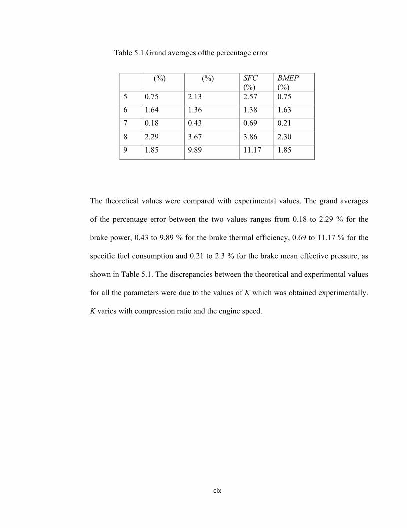
cix
Table 5.1.Grand averages ofthe percentage error
The theoretical values were compared with experimental values. The grand averages
of the percentage error between the two values ranges from 0.18 to 2.29 % for the
brake power, 0.43 to 9.89 % for the brake thermal efficiency, 0.69 to 11.17 % for the
specific fuel consumption and 0.21 to 2.3 % for the brake mean effective pressure, as
shown in Table 5.1. The discrepancies between the theoretical and experimental values
for all the parameters were due to the values of K which was obtained experimentally.
K varies with compression ratio and the engine speed.
(%) (%) SFC (%)
BMEP(%)
5 0.75 2.13 2.57 0.75
6 1.64 1.36 1.38 1.63
7 0.18 0.43 0.69 0.21
8 2.29 3.67 3.86 2.30
9 1.85 9.89 11.17 1.85
cx
5.2 Conclusions
The general conclusions drawn from the results of this research work are as follows:
1. Increase in compression ratio on the Ricardo variable compression ratio engine
increases the brake power, brake thermal efficiency, brake mean effective pressure and
reduction in the specific fuel consumption. It means that higher compression ratios
make it possible to improve the performance characteristics of spark ignition engines.
2. Increase in the engine speed affects the volumetric efficiency more than when the
compression ratio is increased. Thus, compression ratio has minimal effect on the
volumetric efficiency.
3. The optimum compression ratio corresponding to the maximum brake thermal
efficiency and brake power is 9.
4. The small values of the percentage errors between the theoretical and experimental
values show that there is agreement between the theoretical and experimental
performance characteristics of the engine.
cxi
5.3 Recommendations
The performance characteristics of a four stroke variable compression ratio engine in terms of
the brake power, brake thermal efficiency, brake mean effective pressure and specific fuel
consumption have been investigated with increase in thecompression ratio. Further research
should be conducted to include a numerical modeling of combustion in a spark ignition
variable compression ratio engine.
cxii
REFERENCES
Abdel Rahman, A.A. and Osman, M.M.(1997). Experimental investigation of varying
compression ratio of spark ignition engine working under different Ethanol-
Gasoline fuel blends, International Journal of Energy Research, Kuwait University.
Vol. 21, issue 1, pp. 31-40.
Andreas, B. (2003). Torque Modeling and Control of a Variable Compression Engine.
Performed in Vehicular System.Reg nr: LITH-ISY-EX-3421
Asif, A.M., Jandool, K., Saeed, A.S. and Ali, A.C. (2008).Performance Evaluation of a
Single Cylinder Four Stroke Petrol Engine.Farm machinery institute, National
Agricultural Research Centre, Islamabad, Pakistan.
Chaiyot, D. and Somrat, K. (2005). Experimental Influence of Compression Ratio on to
Performance and Emission of Compressed Natural Gas Retrofit Engine, King
Mongkut’s Institute of Technology North Bangkok.
Eastop, T.D. and McConkey, A. (1995).Applied Thermodynamics For Engineering
Technologists.ELBS with Longman, 5th Edition pp. 420-439.
Haresh, K. and Swagatam.(2008). Comparison of Spark Ignition (SI) and Compression
Ignition (CI) Engines. 2011 Bright Hub Inc.
http://www.brighthub.com/engineering/mechanical/articles/1547.
Heywood J. B. (1988). Internal combustion Engines Fundamentals. McGraw Hill Book Company.
Hillier, V.A.W. and Pittuck, F.W. (1978).Fundamentals of Motor Vehicle Technology.Hutchinson and Co (Publisher) Ltd, London. pp. 44.
cxiii
Jan-Ola, O., Per, T. and Bengt, J. (2002).Compression Ratio Influence on Maximum
Fuelled HCCL Engine, Lund Institute of Technology, Society of Automotive
Engineers, Inc. pp.147.
Jehad, A.A and Mohammad, H.D. (2003).Performance Simulation of a four-stroke engine
with variable stroke length and compression ratio, Department of Mechanical
Engineering, Faculty of Engineering and Technology, University of Jordan, 11942,
Jordan.
Mohit, S. and Lamar, S. (2010). Making more efficient combustion engines.
www.brighthub.com/engineering/mechanical/article/90240.aspx
MechanicalEngineeringSystems Laboratory. (2011).
(www.me.metu.edu.tr/me410/ME410%20Labsheet)
Owoade, M.K. (1971). Performance of the Variable Compression Ratio SI Engine at full
throttle.Final year thesis, Ahmadu Bello University, Zaria.
Philip, H.S. and David, N.W.(1954).The Design and Tuning of Competition Engines.
Bentley publisher, 6th edition. ISBN 0837601401
Piston Engine Power Plant.Battery and Energy Technologies, Wood bank Communication
Ltd. United Kingdom. (2005).
Power Supply in Nigeria.(2011).A review of the Nigerian Energy Industry.
www.sweetcrudereports.com/2011/power
Ratnakara, R, Ramachandra R.V. and Muralidhara, M. (2009).Optimising the ratio for a
Mahua fuelled compression ignition engine, India College of Engineering. Vol.4, No.
3.
cxiv
Reciprocating Internal Combustion Engines.(2004). Chapter 6.pp.
224.www.personal.utulsa.edu/kenneth-weston/chapter6.pdf
Reaz M. (2001). Internal Combustion Engines, Engine Classification, Advantages and
Disadvantages. ME 267: Fundamental of Mechanical Engineering Department of
Mechanical Engineering, BUET (teacher.buet.ac.bd/nusairh/res/default/iceth.pdf)
Singer, C.J. and Raper, R. (1999).The Internal Combustion Engine.Clarendom Press. pp. 157 -176
Thermal Efficiency of Engines. (1998). The Japan Society of Mechanical Engineers.www.jsme.or.jp/English/jsme%20roadmap/No.7pdf
Yuh, M. and Tohru, G. (2005).The Effect of Higher Compression Ratio in Two-Stroke Engines. Yamaha Motor Co, Ltd.
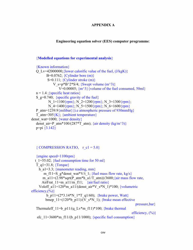
cxv
APPENDIX A
Engineering equation solver (EES) computer programme:
{Modelled equations for experimental analysis}
{Known information}Q_Lv=42000000;{lower calorific value of the fuel, (J/kgK)} B=0.0762; {Cylinder bore (m)}
S=0.111; {Cylinder stroke (m)} V_s=p*B^2*S/4; {Swept volume (m^3)} V=0.00005; {m^3}{volume of the fuel consumed, 50ml} n = 1.4 ;{specific heat ratios}
S_g=0.740; {specific gravity of the fuel} N_1=1100{rpm}; N_2=1200{rpm}; N_3=1300{rpm};
N_4=1400{rpm}; N_5=1500{rpm}; N_6=1600{rpm}P_atm=1239.9{milibar}{i.e atmospheric pressure of 930mmHg}T_atm=305{K}; {ambient temperature}
denst_wat=1000; {water density}denst_air=P_atm*100/(287*T_atm); {air density (kg/m^3)}p=pi {3.142}
{ COMPRESSION RATIO, r_c1 = 5.0}
{engine speed=1100rpm} t_1=55.02; {fuel consumption time for 50 ml} T_q1=31.8; {Torque} h_a1=3.3; {manometer reading, mm}
m_f11=S_g*denst_wat*V/t_1; {fuel mass flow rate, kg/s} m_a11=(2.98*sqrt(P_atm*h_a1/T_atm))/3600;{air mass flow rate, AirFrat_11=m_a11/m_f11; {air/fuel ratio}
Voleff_a11=120*m_a11/(denst_air*V_s*N_1)*100; {volumetricefficiency,(%)}
b_p11=(2*3.14*N_1*T_q1/60); {brake power, Watt} bmep_11=(120*b_p11)/(V_s*N_1); {brake mean effective
pressure,bar}Thermaleff_11=b_p11/(q_Lv*m_f11)*100; {brake thermal
efficiency, (%)}sfc_11=3600*m_f11/(b_p11/1000); {specific fuel consumption}
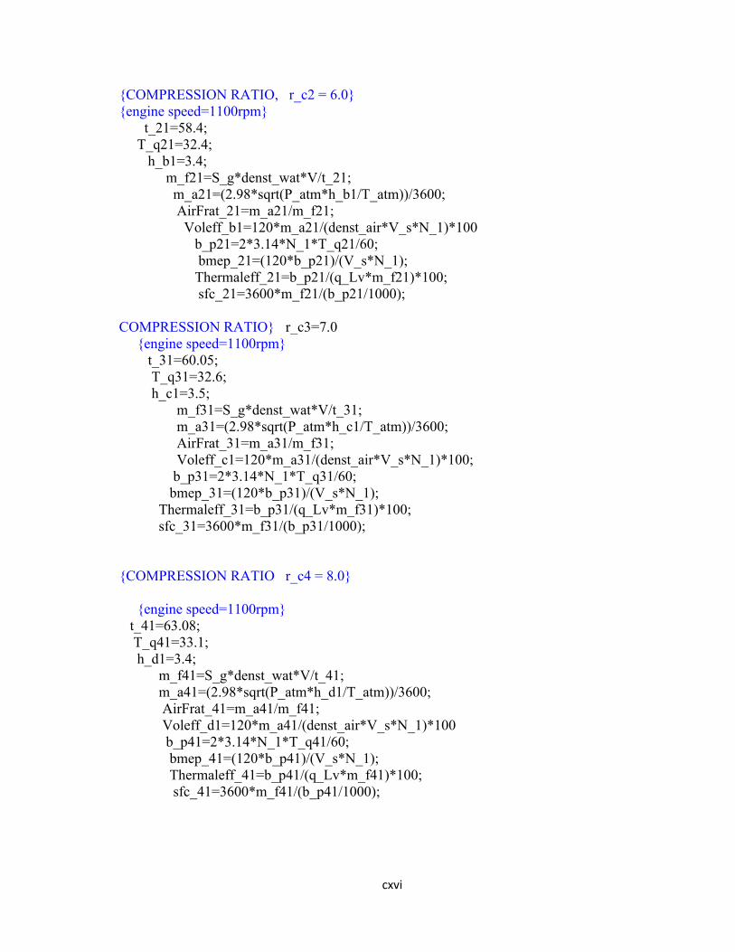
cxvi
{COMPRESSION RATIO, r_c2 = 6.0}{engine speed=1100rpm} t_21=58.4; T_q21=32.4; h_b1=3.4;
m_f21=S_g*denst_wat*V/t_21; m_a21=(2.98*sqrt(P_atm*h_b1/T_atm))/3600; AirFrat_21=m_a21/m_f21; Voleff_b1=120*m_a21/(denst_air*V_s*N_1)*100 b_p21=2*3.14*N_1*T_q21/60; bmep_21=(120*b_p21)/(V_s*N_1); Thermaleff_21=b_p21/(q_Lv*m_f21)*100; sfc_21=3600*m_f21/(b_p21/1000);
COMPRESSION RATIO} r_c3=7.0 {engine speed=1100rpm}
t_31=60.05; T_q31=32.6; h_c1=3.5;
m_f31=S_g*denst_wat*V/t_31; m_a31=(2.98*sqrt(P_atm*h_c1/T_atm))/3600; AirFrat_31=m_a31/m_f31; Voleff_c1=120*m_a31/(denst_air*V_s*N_1)*100; b_p31=2*3.14*N_1*T_q31/60; bmep_31=(120*b_p31)/(V_s*N_1); Thermaleff_31=b_p31/(q_Lv*m_f31)*100; sfc_31=3600*m_f31/(b_p31/1000);
{COMPRESSION RATIO r_c4 = 8.0}
{engine speed=1100rpm} t_41=63.08; T_q41=33.1; h_d1=3.4;
m_f41=S_g*denst_wat*V/t_41; m_a41=(2.98*sqrt(P_atm*h_d1/T_atm))/3600; AirFrat_41=m_a41/m_f41; Voleff_d1=120*m_a41/(denst_air*V_s*N_1)*100 b_p41=2*3.14*N_1*T_q41/60; bmep_41=(120*b_p41)/(V_s*N_1); Thermaleff_41=b_p41/(q_Lv*m_f41)*100; sfc_41=3600*m_f41/(b_p41/1000);
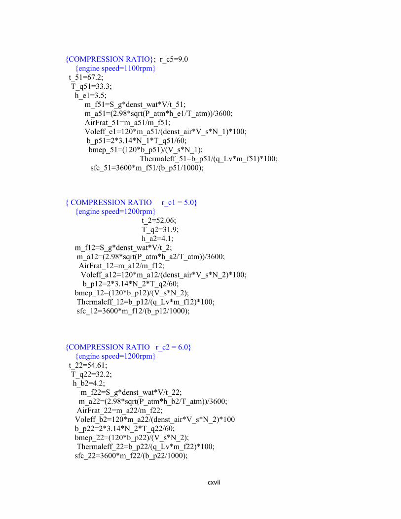
cxvii
{COMPRESSION RATIO}; r_c5=9.0{engine speed=1100rpm}
t_51=67.2; T_q51=33.3; h_e1=3.5;
m_f51=S_g*denst_wat*V/t_51; m_a51=(2.98*sqrt(P_atm*h_e1/T_atm))/3600; AirFrat_51=m_a51/m_f51; Voleff_e1=120*m_a51/(denst_air*V_s*N_1)*100; b_p51=2*3.14*N_1*T_q51/60; bmep_51=(120*b_p51)/(V_s*N_1); Thermaleff_51=b_p51/(q_Lv*m_f51)*100; sfc_51=3600*m_f51/(b_p51/1000);
{ COMPRESSION RATIO r_c1 = 5.0}{engine speed=1200rpm}
t_2=52.06; T_q2=31.9; h_a2=4.1;
m_f12=S_g*denst_wat*V/t_2; m_a12=(2.98*sqrt(P_atm*h_a2/T_atm))/3600; AirFrat_12=m_a12/m_f12; Voleff_a12=120*m_a12/(denst_air*V_s*N_2)*100; b_p12=2*3.14*N_2*T_q2/60; bmep_12=(120*b_p12)/(V_s*N_2); Thermaleff_12=b_p12/(q_Lv*m_f12)*100; sfc_12=3600*m_f12/(b_p12/1000);
{COMPRESSION RATIO r_c2 = 6.0}{engine speed=1200rpm}
t_22=54.61; T_q22=32.2; h_b2=4.2;
m_f22=S_g*denst_wat*V/t_22; m_a22=(2.98*sqrt(P_atm*h_b2/T_atm))/3600; AirFrat_22=m_a22/m_f22; Voleff_b2=120*m_a22/(denst_air*V_s*N_2)*100b_p22=2*3.14*N_2*T_q22/60; bmep_22=(120*b_p22)/(V_s*N_2); Thermaleff_22=b_p22/(q_Lv*m_f22)*100; sfc_22=3600*m_f22/(b_p22/1000);
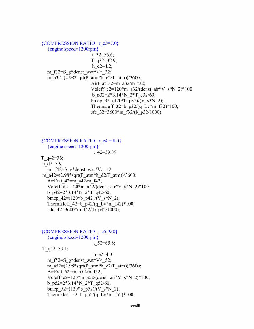
cxviii
{COMPRESSION RATIO r_c3=7.0}{engine speed=1200rpm}
t_32=56.6; T_q32=32.9; h_c2=4.2;
m_f32=S_g*denst_wat*V/t_32; m_a32=(2.98*sqrt(P_atm*h_c2/T_atm))/3600; AirFrat_32=m_a32/m_f32; Voleff_c2=120*m_a32/(denst_air*V_s*N_2)*100 b_p32=2*3.14*N_2*T_q32/60; bmep_32=(120*b_p32)/(V_s*N_2); Thermaleff_32=b_p32/(q_Lv*m_f32)*100; sfc_32=3600*m_f32/(b_p32/1000);
{COMPRESSION RATIO r_c4 = 8.0}{engine speed=1200rpm}
t_42=59.89; T_q42=33; h_d2=3.9;
m_f42=S_g*denst_wat*V/t_42; m_a42=(2.98*sqrt(P_atm*h_d2/T_atm))/3600;
AirFrat_42=m_a42/m_f42;Voleff_d2=120*m_a42/(denst_air*V_s*N_2)*100b_p42=2*3.14*N_2*T_q42/60; bmep_42=(120*b_p42)/(V_s*N_2); Thermaleff_42=b_p42/(q_Lv*m_f42)*100; sfc_42=3600*m_f42/(b_p42/1000);
{COMPRESSION RATIO r_c5=9.0}{engine speed=1200rpm}
t_52=65.8; T_q52=33.1; h_e2=4.3;
m_f52=S_g*denst_wat*V/t_52; m_a52=(2.98*sqrt(P_atm*h_e2/T_atm))/3600; AirFrat_52=m_a52/m_f52;Voleff_e2=120*m_a52/(denst_air*V_s*N_2)*100;b_p52=2*3.14*N_2*T_q52/60; bmep_52=(120*b_p52)/(V_s*N_2); Thermaleff_52=b_p52/(q_Lv*m_f52)*100;
cxix
sfc_52=3600*m_f52/(b_p52/1000);
{ COMPRESSION RATIO r_c1 = 5.0}{engine speed=1300rpm}
t_3=50.1; T_q3=31.5;h_a3=4.7;
m_f13=S_g*denst_wat*V/t_3; m_a13=(2.98*sqrt(P_atm*h_a3/T_atm))/3600; AirFrat_13=m_a13/m_f13; Voleff_a13=120*m_a13/(denst_air*V_s*N_3)*100; b_p13=2*3.14*N_3*T_q3/60; bmep_13=(120*b_p13)/(V_s*N_3); Thermaleff_13=b_p13/(q_Lv*m_f13)*100; sfc_13=3600*m_f13/(b_p13/1000);
{COMPRESSION RATIO r_c2 = 6.0}{engine speed=1300rpm}
t_23=53.98;T_q23=32.1;h_b3=4.9;
m_f23=S_g*denst_wat*V/t_23; m_a23=(2.98*sqrt(P_atm*h_b3/T_atm))/3600; AirFrat_23=m_a23/m_f23;Voleff_b3=120*m_a23/(denst_air*V_s*N_3)*100b_p23=2*3.14*N_3*T_q23/60; bmep_23=(120*b_p23)/(V_s*N_3); Thermaleff_23=b_p23/(q_Lv*m_f23)*100; sfc_23=3600*m_f23/(b_p23/1000);
{COMPRESSION RATIO r_c3=7.0}{engine speed=1300rpm}
t_33=55.03; T_q33=32.2;h_c3=4.9;
m_f33=S_g*denst_wat*V/t_33; m_a33=(2.98*sqrt(P_atm*h_c3/T_atm))/3600; AirFrat_33=m_a33/m_f33; Voleff_c3=120*m_a33/(denst_air*V_s*N_3)*100b_p33=2*3.14*N_3*T_q33/60; bmep_33=(120*b_p33)/(V_s*N_3); Thermaleff_33=b_p33/(q_Lv*m_f33)*100; sfc_33=3600*m_f33/(b_p33/1000);
cxx
{COMPRESSION RATIO r_c4 = 8.0}{engine speed=1300rpm}
t_43=58.38; T_q43=32.9; h_d3=4.9;
m_f43=S_g*denst_wat*V/t_43; m_a43=(2.98*sqrt(P_atm*h_d3/T_atm))/3600; AirFrat_43=m_a43/m_f43; Voleff_d3=120*m_a43/(denst_air*V_s*N_3)*100 b_p43=2*3.14*N_3*T_q43/60; bmep_43=(120*b_p43)/(V_s*N_3); Thermaleff_43=b_p43/(q_Lv*m_f43)*100; sfc_43=3600*m_f43/(b_p43/1000);
{COMPRESSION RATIO r_c5=9.0}{engine speed=1300rpm}
t_53=64.1; T_q53=32.9; h_e3=5.5;
m_f53=S_g*denst_wat*V/t_53; m_a53=(2.98*sqrt(P_atm*h_e3/T_atm))/3600; AirFrat_53=m_a53/m_f53; Voleff_e3=120*m_a53/(denst_air*V_s*N_3)*100; b_p53=2*3.14*N_3*T_q53/60; bmep_53=(120*b_p53)/(V_s*N_3); Thermaleff_53=b_p53/(q_Lv*m_f53)*100; sfc_53=3600*m_f53/(b_p53/1000);
{ COMPRESSION RATIO r_c1 = 5.0}{engine speed=1400rpm}
t_4=48.1;T_q4=30.1; h_a4=5.2;
m_f14=S_g*denst_wat*V/t_4; m_a14=(2.98*sqrt(P_atm*h_a4/T_atm))/3600;AirFrat_14=m_a14/m_f14;Voleff_a14=120*m_a14/(denst_air*V_s*N_4)*100b_p14=2*3.14*N_4*T_q4/60; bmep_14=(120*b_p14)/(V_s*N_4);
cxxi
Thermaleff_14=b_p14/(q_Lv*m_f14)*100; sfc_14=3600*m_f14/(b_p14/1000);
{COMPRESSION RATIO r_c2 = 6.0}{engine speed=1400rpm}
t_24=51.22; T_q24=31; h_b4=5.3;
m_f24=S_g*denst_wat*V/t_24; m_a24=(2.98*sqrt(P_atm*h_b4/T_atm))/3600; AirFrat_24=m_a24/m_f24; Voleff_b4=120*m_a24/(denst_air*V_s*N_4)*100 b_p24=2*3.14*N_4*T_q24/60; bmep_24=(120*b_p24)/(V_s*N_4); Thermaleff_24=b_p24/(q_Lv*m_f24)*100; sfc_24=3600*m_f24/(b_p24/1000);
{COMPRESSION RATIO r_c3=7.0}{engine speed=1400rpm}
t_34=53.9; T_q34=31.5; h_c4=5.3;
m_f34=S_g*denst_wat*V/t_34; m_a34=(2.98*sqrt(P_atm*h_c4/T_atm))/3600; AirFrat_34=m_a34/m_f34;Voleff_c4=120*m_a34/(denst_air*V_s*N_4)*100b_p34=2*3.14*N_4*T_q34/60; bmep_34=(120*b_p34)/(V_s*N_4); Thermaleff_34=b_p34/(q_Lv*m_f34)*100; sfc_34=3600*m_f34/(b_p34/1000);
{COMPRESSION RATIO r_c4 = 8.0}{engine speed=1400rpm} t_44=58.22; T_q44=31.6; h_d4=5.5;
m_f44=S_g*denst_wat*V/t_44; m_a44=(2.98*sqrt(P_atm*h_d4/T_atm))/3600; AirFrat_44=m_a44/m_f44;Voleff_d4=120*m_a44/(denst_air*V_s*N_4)*100 b_p44=2*3.14*N_4*T_q44/60; bmep_44=(120*b_p44)/(V_s*N_4); Thermaleff_44=b_p44/(q_Lv*m_f44)*100;
cxxii
sfc_44=3600*m_f44/(b_p44/1000);
{COMPRESSION RATIO r_c5=9.0}{engine speed=1400rpm}
t_54=62.8; T_q54=31.7; h_e4=5.7;
m_f54=S_g*denst_wat*V/t_54; m_a54=(2.98*sqrt(P_atm*h_e4/T_atm))/3600; AirFrat_54=m_a54/m_f54;Voleff_e4=120*m_a54/(denst_air*V_s*N_4)*100;b_p54=2*3.14*N_4*T_q54/60; bmep_54=(120*b_p54)/(V_s*N_4); Thermaleff_54=b_p54/(q_Lv*m_f54)*100; sfc_54=3600*m_f54/(b_p54/1000);
{ COMPRESSION RATIO r_c1 = 5.0}{engine speed=1500rpm}
t_5=44.5;T_q5=28.9; h_a5=5.5;
m_f15=S_g*denst_wat*V/t_5; m_a15=(2.98*sqrt(P_atm*h_a5/T_atm))/3600; AirFrat_15=m_a15/m_f15;Voleff_a15=120*m_a15/(denst_air*V_s*N_5)*100b_p15=2*3.14*N_5*T_q5/60; bmep_15=(120*b_p15)/(V_s*N_5); Thermaleff_15=b_p15/(q_Lv*m_f15)*100; sfc_15=3600*m_f15/(b_p15/1000);
{COMPRESSION RATIO r_c2 = 6.0}{engine speed=1500rpm}
t_25=48.67;T_q25=29.5; h_b5=5.6;
m_f25=S_g*denst_wat*V/t_25; m_a25 =(2.98*sqrt(P_atm*h_b5/T_atm))/3600; AirFrat_25=m_a25/m_f25;Voleff_b5=120*m_a25/(denst_air*V_s*N_5)*100b_p25=2*3.14*N_5*T_q25/60;
cxxiii
bmep_25=(120*b_p25)/(V_s*N_5); Thermaleff_25=b_p25/(q_Lv*m_f25)*100; sfc_25=3600*m_f25/(b_p25/1000);
{COMPRESSION RATIO r_c3=7.0}{engine speed=1500rpm}
t_35=50.13; T_q35=30.1; h_c5=5.8;
m_f35=S_g*denst_wat*V/t_35; m_a35=(2.98*sqrt(P_atm*h_c5/T_atm))/3600; AirFrat_35=m_a35/m_f35; Voleff_c5=120*m_a35/(denst_air*V_s*N_5)*100 b_p35=2*3.14*N_5*T_q35/60; bmep_35=(120*b_p35)/(V_s*N_5); Thermaleff_35=b_p35/(q_Lv*m_f35)*100; sfc_35=3600*m_f35/(b_p35/1000);
{COMPRESSION RATIO r_c4 = 8.0}{engine speed=1500rpm}
t_45=53.6; T_q45=30.5; h_d5=6.0;
m_f45=S_g*denst_wat*V/t_45; m_a45=(2.98*sqrt(P_atm*h_d5/T_atm))/3600; AirFrat_45=m_a45/m_f45;Voleff_d5=120*m_a45/(denst_air*V_s*N_5)*100b_p45=2*3.14*N_5*T_q45/60; bmep_45=(120*b_p45)/(V_s*N_5); Thermaleff_45=b_p45/(q_Lv*m_f45)*100; sfc_45=3600*m_f45/(b_p45/1000);
{COMPRESSION RATIO r_c5=9.0}{engine speed=1500rpm}
t_55=61.2 T_q55=30.7; h_e5=6.1;
m_f55=S_g*denst_wat*V/t_55; m_a55=(2.98*sqrt(P_atm*h_e5/T_atm))/3600; AirFrat_55=m_a55/m_f55;Voleff_e5=120*m_a55/(denst_air*V_s*N_5)*100; b_p55=2*3.14*N_5*T_q55/60;
cxxiv
bmep_55=(120*b_p55)/(V_s*N_5); Thermaleff_55=b_p55/(q_Lv*m_f55)*100;sfc_55=3600*m_f55/(b_p55/1000);
{COMPRESSION RATIO r_c1 = 5.0}{engine speed=1600rpm}
t_6=40.3; T_q6=27.4; h_a6=5.7;
m_f16=S_g*denst_wat*V/t_6; m_a16=(2.98*sqrt(P_atm*h_a6/T_atm))/3600; AirFrat_16=m_a16/m_f16;Voleff_a16=120*m_a16/(denst_air*V_s*N_6)*100b_p16=2*3.14*N_6*T_q6/60; bmep_16=(120*b_p16)/(V_s*N_6); Thermaleff_16=b_p16/(q_Lv*m_f16)*100; sfc_16=3600*m_f16/(b_p16/1000);
{COMPRESSION RATIO r_c2 = 6.0}{engine speed=1600rpm}
t_26=45.2; T_q26=27.9; h_b6=5.9;
m_f26=S_g*denst_wat*V/t_26; m_a26=(2.98*sqrt(P_atm*h_b6/T_atm))/3600; AirFrat_26=m_a26/m_f26;Voleff_b6=120*m_a26/(denst_air*V_s*N_6)*100b_p26=2*3.14*N_6*T_q26/60; bmep_26=(120*b_p26)/(V_s*N_6); Thermaleff_26=b_p26/(q_Lv*m_f26)*100; sfc_26=3600*m_f26/(b_p26/1000);
{COMPRESSION RATIO r_c3=7.0}{engine speed=1600rpm}
t_36=46.5;T_q36=28.4; h_c6=6.1;
m_f36=S_g*denst_wat*V/t_36; m_a36=(2.98*sqrt(P_atm*h_c6/T_atm))/3600; AirFrat_36=m_a36/m_f36;Voleff_c6=120*m_a36/(denst_air*V_s*N_6)*100b_p36=2*3.14*N_6*T_q36/60; bmep_36=(120*b_p36)/(V_s*N_6);
cxxv
Thermaleff_36=b_p36/(q_Lv*m_f36)*100; sfc_36=3600*m_f36/(b_p36/1000);
{COMPRESSION RATIO r_c4 = 8.0}{engine speed=1600rpm}
t_46=52.2; T_q46=28.6;
h_d6=6.2;
m_f46=S_g*denst_wat*V/t_46; m_a46=(2.98*sqrt(P_atm*h_d6/T_atm))/3600;
AirFrat_46=m_a46/m_f46;Voleff_d6=120*m_a46/(denst_air*V_s*N_6)*100; b_p46=2*3.14*N_6*T_q46/60; bmep_46=(120*b_p46)/(V_s*N_6); Thermaleff_46=b_p46/(q_Lv*m_f46)*100; sfc_46=3600*m_f46/(b_p46/1000);
{COMPRESSION RATIO r_c5=9.0}{engine speed=1600rpm}
t_56=58.8; T_q56=29.1; h_e6=6.6;
m_f56=S_g*denst_wat*V/t_56; m_a56=(2.98*sqrt(P_atm*h_e6/T_atm))/3600; AirFrat_56=m_a56/m_f56; Voleff_e6=120*m_a56/(denst_air*V_s*N_6)*100; b_p56=2*3.14*N_6*T_q56/60; bmep_56=(120*b_p56)/(V_s*N_6); Thermaleff_56=b_p56/(q_Lv*m_f56)*100; sfc_56=3600*m_f56/(b_p56/1000)
{Calculation of 'K' for the reference compression ratio of 7.0, usingequation 3.13} T_q31 = (K_1/(2*p))*(1-1/(r_c3^(n-1)))*(m_f31*Q_Lv/(N_1/60));
T_q32 = (K_2/(2*p))*(1-1/(r_c3^(n-1)))*(m_f32*Q_Lv/(N_2/60));
T_q33 = (K_3/(2*p))*(1-1/(r_c3^(n-1)))*(m_f33*Q_Lv/(N_3/60));
T_q34 = (K_4/(2*p))*(1-1/(r_c3^(n-1)))*(m_f34*Q_Lv/(N_4/60));
T_q35 = (K_5/(2*p))*(1-1/(r_c3^(n-1)))*(m_f35*Q_Lv/(N_5/60));
T_q36 = (K_36/(2*p))*(1-1/(r_c3^(n-1)))*(m_f36*Q_Lv/(N_6/60));
cxxvi
APPENDIX B
Engineering equation solver (EES) computer programme:
{Modelled equations for theoretical analysis}
{Reference r_C= 7.0}
{Known values}Q_Lv=42000000; {lower calorific value of the fuel (J/kgK)} B=0.0762; {Cylinder bore (m)} S=0.111; {Cylinder stroke (m)} V_s=p*B^2*S/4; {Swept volume (m^3)} N_1=1100{rpm}; N_2=1200{rpm}; N_3=1300{rpm}; N_4=1400{rpm}; N_5=1500{rpm}; N_6=1600{rpm}; {engine speed T_q1=32.6; T_q2=32.9; T_q3=32.2; T_q4=31.5; T_q5=30.1; T_q6=28.4;{Brake torque from reference compression ratio of 7}
{COMPRESSION RATIO, r_c1=5.0}{engine speed=1100rpm} T_q11=T_q1-(5/7)^0.4; B_p11=2*3.14*N_1*T_q11/60 T_q11=K_1/(2*3.14)*(1-(1/5^0.4))*60*m_f11*Q_Lv/N_1 BMEP_11=120*B_p11/(V_s*N_1) THERMALEFF_11=B_p11/(Q_Lv*m_f11) SFC_11=3600*m_f11/(B_p11/1000)
{COMPRESSION RATIO, r_c2=6.0} {engine speed=1100rpm} T_q21=T_q1-(6/7)^0.4;; B_p21=2*3.14*N_1*T_q21/60 T_q21=K_1/(2*3.14)*(1-(1/6^0.4))*60*m_f21*Q_Lv/N_1 BMEP_21=120*B_p21/(V_s*N_1) THERMALEFF_21=B_p21/(Q_Lv*m_f21) SFC_21=3600*m_f21/(B_p21/1000)
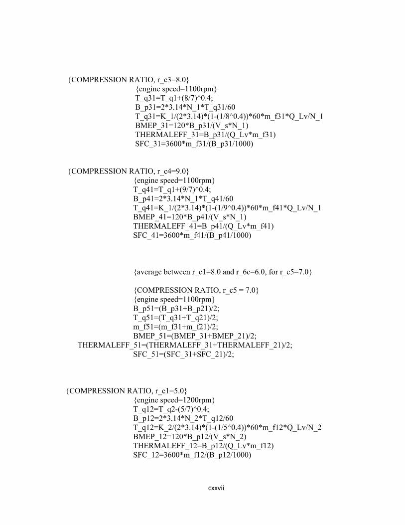
cxxvii
{COMPRESSION RATIO, r_c3=8.0} {engine speed=1100rpm} T_q31=T_q1+(8/7)^0.4; B_p31=2*3.14*N_1*T_q31/60 T_q31=K_1/(2*3.14)*(1-(1/8^0.4))*60*m_f31*Q_Lv/N_1 BMEP_31=120*B_p31/(V_s*N_1) THERMALEFF_31=B_p31/(Q_Lv*m_f31) SFC_31=3600*m_f31/(B_p31/1000)
{COMPRESSION RATIO, r_c4=9.0} {engine speed=1100rpm} T_q41=T_q1+(9/7)^0.4; B_p41=2*3.14*N_1*T_q41/60 T_q41=K_1/(2*3.14)*(1-(1/9^0.4))*60*m_f41*Q_Lv/N_1 BMEP_41=120*B_p41/(V_s*N_1) THERMALEFF_41=B_p41/(Q_Lv*m_f41) SFC_41=3600*m_f41/(B_p41/1000)
{average between r_c1=8.0 and r_6c=6.0, for r_c5=7.0}
{COMPRESSION RATIO, r_c5 = 7.0} {engine speed=1100rpm} B_p51=(B_p31+B_p21)/2; T_q51=(T_q31+T_q21)/2; m_f51=(m_f31+m_f21)/2; BMEP_51=(BMEP_31+BMEP_21)/2; THERMALEFF_51=(THERMALEFF_31+THERMALEFF_21)/2; SFC_51=(SFC_31+SFC_21)/2;
{COMPRESSION RATIO, r_c1=5.0} {engine speed=1200rpm} T_q12=T_q2-(5/7)^0.4; B_p12=2*3.14*N_2*T_q12/60 T_q12=K_2/(2*3.14)*(1-(1/5^0.4))*60*m_f12*Q_Lv/N_2 BMEP_12=120*B_p12/(V_s*N_2) THERMALEFF_12=B_p12/(Q_Lv*m_f12) SFC_12=3600*m_f12/(B_p12/1000)
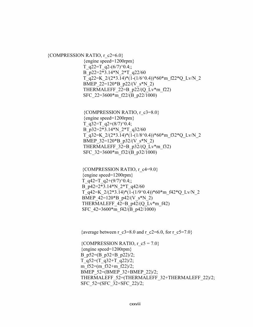
cxxviii
{COMPRESSION RATIO, r_c2=6.0} {engine speed=1200rpm} T_q22=T_q2-(6/7)^0.4;; B_p22=2*3.14*N_2*T_q22/60 T_q22=K_2/(2*3.14)*(1-(1/6^0.4))*60*m_f22*Q_Lv/N_2 BMEP_22=120*B_p22/(V_s*N_2) THERMALEFF_22=B_p22/(Q_Lv*m_f22) SFC_22=3600*m_f22/(B_p22/1000)
{COMPRESSION RATIO, r_c3=8.0} {engine speed=1200rpm} T_q32=T_q2+(8/7)^0.4; B_p32=2*3.14*N_2*T_q32/60 T_q32=K_2/(2*3.14)*(1-(1/8^0.4))*60*m_f32*Q_Lv/N_2 BMEP_32=120*B_p32/(V_s*N_2) THERMALEFF_32=B_p32/(Q_Lv*m_f32) SFC_32=3600*m_f32/(B_p32/1000)
{COMPRESSION RATIO, r_c4=9.0} {engine speed=1200rpm} T_q42=T_q2+(9/7)^0.4;; B_p42=2*3.14*N_2*T_q42/60 T_q42=K_2/(2*3.14)*(1-(1/9^0.4))*60*m_f42*Q_Lv/N_2 BMEP_42=120*B_p42/(V_s*N_2) THERMALEFF_42=B_p42/(Q_Lv*m_f42) SFC_42=3600*m_f42/(B_p42/1000)
{average between r_c3=8.0 and r_c2=6.0, for r_c5=7.0}
{COMPRESSION RATIO, r_c5 = 7.0} {engine speed=1200rpm} B_p52=(B_p32+B_p22)/2; T_q52=(T_q32+T_q22)/2; m_f52=(m_f32+m_f22)/2; BMEP_52=(BMEP_32+BMEP_22)/2; THERMALEFF_52=(THERMALEFF_32+THERMALEFF_22)/2; SFC_52=(SFC_32+SFC_22)/2;
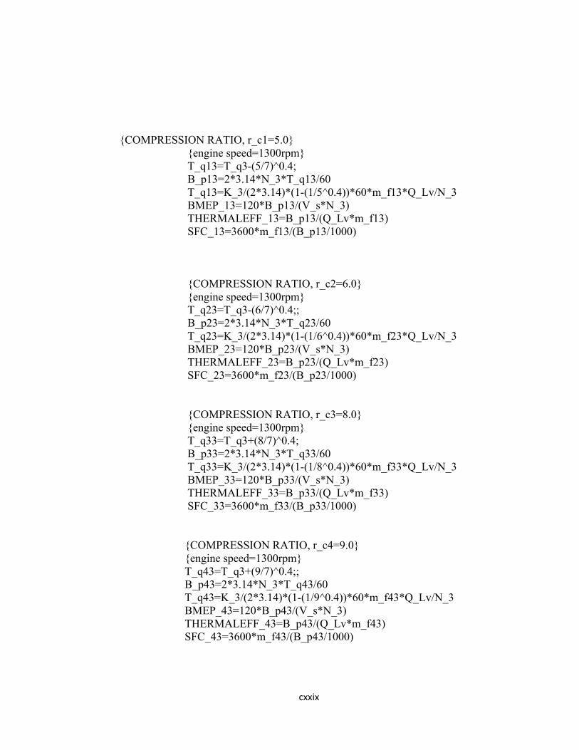
cxxix
{COMPRESSION RATIO, r_c1=5.0} {engine speed=1300rpm} T_q13=T_q3-(5/7)^0.4; B_p13=2*3.14*N_3*T_q13/60 T_q13=K_3/(2*3.14)*(1-(1/5^0.4))*60*m_f13*Q_Lv/N_3 BMEP_13=120*B_p13/(V_s*N_3) THERMALEFF_13=B_p13/(Q_Lv*m_f13) SFC_13=3600*m_f13/(B_p13/1000)
{COMPRESSION RATIO, r_c2=6.0} {engine speed=1300rpm} T_q23=T_q3-(6/7)^0.4;; B_p23=2*3.14*N_3*T_q23/60 T_q23=K_3/(2*3.14)*(1-(1/6^0.4))*60*m_f23*Q_Lv/N_3 BMEP_23=120*B_p23/(V_s*N_3) THERMALEFF_23=B_p23/(Q_Lv*m_f23) SFC_23=3600*m_f23/(B_p23/1000)
{COMPRESSION RATIO, r_c3=8.0} {engine speed=1300rpm} T_q33=T_q3+(8/7)^0.4; B_p33=2*3.14*N_3*T_q33/60 T_q33=K_3/(2*3.14)*(1-(1/8^0.4))*60*m_f33*Q_Lv/N_3 BMEP_33=120*B_p33/(V_s*N_3) THERMALEFF_33=B_p33/(Q_Lv*m_f33) SFC_33=3600*m_f33/(B_p33/1000)
{COMPRESSION RATIO, r_c4=9.0} {engine speed=1300rpm} T_q43=T_q3+(9/7)^0.4;; B_p43=2*3.14*N_3*T_q43/60 T_q43=K_3/(2*3.14)*(1-(1/9^0.4))*60*m_f43*Q_Lv/N_3 BMEP_43=120*B_p43/(V_s*N_3) THERMALEFF_43=B_p43/(Q_Lv*m_f43) SFC_43=3600*m_f43/(B_p43/1000)
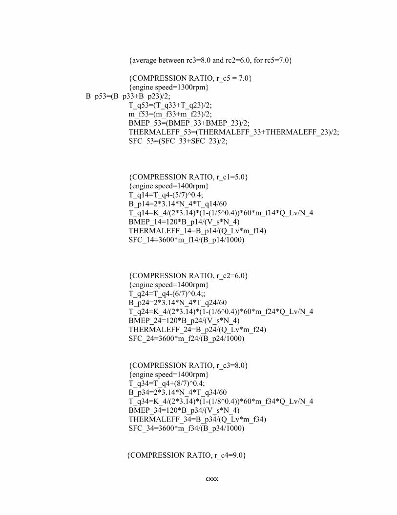
cxxx
{average between rc3=8.0 and rc2=6.0, for rc5=7.0}
{COMPRESSION RATIO, r_c5 = 7.0} {engine speed=1300rpm} B_p53=(B_p33+B_p23)/2; T_q53=(T_q33+T_q23)/2; m_f53=(m_f33+m_f23)/2; BMEP_53=(BMEP_33+BMEP_23)/2; THERMALEFF_53=(THERMALEFF_33+THERMALEFF_23)/2; SFC_53=(SFC_33+SFC_23)/2;
{COMPRESSION RATIO, r_c1=5.0} {engine speed=1400rpm} T_q14=T_q4-(5/7)^0.4; B_p14=2*3.14*N_4*T_q14/60 T_q14=K_4/(2*3.14)*(1-(1/5^0.4))*60*m_f14*Q_Lv/N_4 BMEP_14=120*B_p14/(V_s*N_4) THERMALEFF_14=B_p14/(Q_Lv*m_f14) SFC_14=3600*m_f14/(B_p14/1000)
{COMPRESSION RATIO, r_c2=6.0} {engine speed=1400rpm} T_q24=T_q4-(6/7)^0.4;; B_p24=2*3.14*N_4*T_q24/60 T_q24=K_4/(2*3.14)*(1-(1/6^0.4))*60*m_f24*Q_Lv/N_4 BMEP_24=120*B_p24/(V_s*N_4) THERMALEFF_24=B_p24/(Q_Lv*m_f24) SFC_24=3600*m_f24/(B_p24/1000)
{COMPRESSION RATIO, r_c3=8.0} {engine speed=1400rpm} T_q34=T_q4+(8/7)^0.4; B_p34=2*3.14*N_4*T_q34/60 T_q34=K_4/(2*3.14)*(1-(1/8^0.4))*60*m_f34*Q_Lv/N_4 BMEP_34=120*B_p34/(V_s*N_4) THERMALEFF_34=B_p34/(Q_Lv*m_f34) SFC_34=3600*m_f34/(B_p34/1000)
{COMPRESSION RATIO, r_c4=9.0}
cxxxi
{engine speed=1400rpm} T_q44=T_q4+(9/7)^0.4; B_p44=2*3.14*N_4*T_q44/60 T_q44=K_4/(2*3.14)*(1-(1/9^0.4))*60*m_f44*Q_Lv/N_4 BMEP_44=120*B_p44/(V_s*N_4) THERMALEFF_44=B_p44/(Q_Lv*m_f44) SFC_44=3600*m_f44/(B_p44/1000)
{average between rc3=8.0 and rc2=6.0, for rc5=7.0}
{COMPRESSION RATIO, r_c5 = 7.0} {engine speed=1400rpm} B_p54=(B_p34+B_p24)/2; T_q54=(T_q34+T_q24)/2; m_f54=(m_f34+m_f24)/2; BMEP_54=(BMEP_34+BMEP_24)/2; THERMALEFF_54=(THERMALEFF_34+THERMALEFF_24)/2; SFC_54=(SFC_34+SFC_24)/2;
{COMPRESSION RATIO, r_c1=5.0} {engine speed=1500rpm} T_q15=T_q5-(5/7)^0.4; B_p15=2*3.14*N_5*T_q15/60 T_q15=K_5/(2*3.14)*(1-(1/5^0.4))*60*m_f15*Q_Lv/N_5 BMEP_15=120*B_p15/(V_s*N_5) THERMALEFF_15=B_p15/(Q_Lv*m_f15) SFC_15=3600*m_f15/(B_p15/1000)
{COMPRESSION RATIO, r_c2=6.0} {engine speed=1500rpm} T_q25=T_q5-(6/7)^0.4;; B_p25=2*3.14*N_5*T_q25/60 T_q25=K_5/(2*3.14)*(1-(1/6^0.4))*60*m_f25*Q_Lv/N_5 BMEP_25=120*B_p25/(V_s*N_5) THERMALEFF_25=B_p25/(Q_Lv*m_f25) SFC_25=3600*m_f25/(B_p25/1000)
{COMPRESSION RATIO, r_c3=8.0} {engine speed=1500rpm} T_q35=T_q5+(8/7)^0.4; B_p35=2*3.14*N_5*T_q35/60
cxxxii
T_q35=K_5/(2*3.14)*(1-(1/8^0.4))*60*m_f35*Q_Lv/N_5 BMEP_35=120*B_p35/(V_s*N_5) THERMALEFF_35=B_p35/(Q_Lv*m_f35) SFC_35=3600*m_f35/(B_p35/1000)
{COMPRESSION RATIO, r_c4=9.0} {engine speed=1500rpm} T_q45=T_q5+(9/7)^0.4;; B_p45=2*3.14*N_5*T_q45/60 T_q45=K_5/(2*3.14)*(1-(1/9^0.4))*60*m_f45*Q_Lv/N_5 BMEP_45=120*B_p45/(V_s*N_5) THERMALEFF_45=B_p45/(Q_Lv*m_f45) SFC_45=3600*m_f45/(B_p45/1000)
{average between rc3=8.0 and rc2=6.0, for rc5=7.0}
{COMPRESSION RATIO, r_c5 = 7.0} {engine speed=1500rpm} B_p55=(B_p35+B_p25)/2; T_q55=(T_q35+T_q25)/2; m_f55=(m_f35+m_f25)/2; BMEP_55=(BMEP_35+BMEP_25)/2; THERMALEFF_55=(THERMALEFF_35+THERMALEFF_25)/2; SFC_55=(SFC_35+SFC_25)/2;
{COMPRESSION RATIO, r_c1=5.0} {engine speed=1600rpm} T_q16=T_q6-(5/7)^0.4; B_p16=2*3.14*N_6*T_q16/60 T_q16=K_6/(2*3.14)*(1-(1/5^0.4))*60*m_f16*Q_Lv/N_6 BMEP_16=120*B_p16/(V_s*N_6) THERMALEFF_16=B_p16/(Q_Lv*m_f16) SFC_16=3600*m_f16/(B_p16/1000)
{COMPRESSION RATIO, r_c2=6.0} {engine speed=1600rpm}
cxxxiii
T_q26=T_q6-(6/7)^0.4; B_p26=2*3.14*N_6*T_q26/60 T_q26=K_6/(2*3.14)*(1-(1/6^0.4))*60*m_f26*Q_Lv/N_6 BMEP_26=120*B_p26/(V_s*N_6) THERMALEFF_26=B_p26/(Q_Lv*m_f26) SFC_26=3600*m_f26/(B_p26/1000)
{COMPRESSION RATIO, r_c3=8.0} {engine speed=1600rpm} T_q36=T_q6+(8/7)^0.4; B_p36=2*3.14*N_6*T_q36/60 T_q36=K_6/(2*3.14)*(1-(1/8^0.4))*60*m_f36*Q_Lv/N_6 BMEP_36=120*B_p36/(V_s*N_6) THERMALEFF_36=B_p36/(Q_Lv*m_f36) SFC_36=3600*m_f36/(B_p36/1000)
{COMPRESSION RATIO, r_c4=9.0} {engine speed=1500rpm} T_q46=T_q6+(9/7)^0.4; B_p46=2*3.14*N_6*T_q46/60 T_q46=K_6/(2*3.14)*(1-(1/9^0.4))*60*m_f46*Q_Lv/N_6 BMEP_46=120*B_p46/(V_s*N_6) THERMALEFF_46=B_p46/(Q_Lv*m_f46) SFC_46=3600*m_f46/(B_p46/1000)
{average between rc=8.0 and rc=6.0, for rc=7.0}
{COMPRESSION RATIO, r_c5 = 7.0} {engine speed=1600rpm} B_p56=(B_p36+B_p26)/2; T_q56=(T_q36+T_q26)/2; m_f56=(m_f36+m_f26)/2; BMEP_56=(BMEP_36+BMEP_26)/2; THERMALEFF_56=(THERMALEFF_36+THERMALEFF_26)/2; SFC_56=(SFC_36+SFC_26)/2;
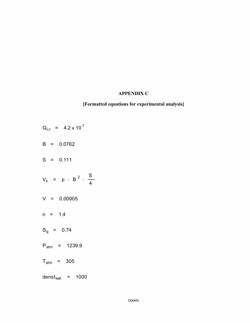
cxxxiv
APPENDIX C
[Formatted equations for experimental analysis]
QLv = 4.2 x 10 7
B = 0.0762
S = 0.111
Vs = p · B2
·S
4
V = 0.00005
n = 1.4
Sg = 0.74
Patm = 1239.9
Tatm = 305
denstwat = 1000
cxxxv
r_c1 = 5
denstair = Patm ·100
287 · Tatm
t1 = 55.02
Tq1 = 31.8
ha1 = 3.3
m f 11 = Sg · denstwat ·V
t1
m a11 =
2.98 · Patm ·ha1
Tatm
3600
AirFrat11 =m a11
m f 11
Voleffa11 = 120 ·m a11
denstair · Vs · N1· 100
bp11 = 2 · 3.14 · N1 ·Tq1
60
bmep11 =120 · bp11
Vs · N1
Thermaleff11 =bp11
QLv · m f 11· 100
cxxxvi
r_c2 = 6
sfc11 = 3600 ·m f 11
bp11
1000
t21 = 58.4
Tq21 = 32.4
hb1 = 3.4
m f 21 = Sg · denstwat ·V
t21
m a21 =
2.98 · Patm ·hb1
Tatm
3600
AirFrat21 =m a21
m f 21
Voleffb1 = 120 ·m a21
denstair · Vs · N1· 100
bp21 = 2 · 3.14 · N1 ·Tq21
60
bmep21 =120 · bp21
Vs · N1
Thermaleff21 =bp21
QLv · m f 21· 100
cxxxvii
r_c3 = 7
sfc21 = 3600 ·m f 21
bp21
1000
t31 = 60.05
Tq31 = 32.6
hc1 = 3.5
m f 31 = Sg · denstwat ·V
t31
m a31 =
2.98 · Patm ·hc1
Tatm
3600
AirFrat31 =m a31
m f 31
Voleffc1 = 120 ·m a31
denstair · Vs · N1· 100
bp31 = 2 · 3.14 · N1 ·Tq31
60
bmep31 =120 · bp31
Vs · N1
Thermaleff31 =bp31
QLv · m f 31· 100

cxxxviii
r_c4 = 8
sfc31 = 3600 ·m f 31
bp31
1000
t41 = 63.08
Tq41 = 33.1
hd1 = 3.4
m f 41 = Sg · denstwat ·V
t41
m a41 =
2.98 · Patm ·hd1
Tatm
3600
AirFrat41 =m a41
m f 41
Voleffd1 = 120 ·m a41
denstair · Vs · N1· 100
bp41 = 2 · 3.14 · N1 ·Tq41
60
bmep41 =120 · bp41
Vs · N1
Thermaleff41 =bp41
QLv · m f 41· 100
cxxxix
r_c5 = 9
sfc41 = 3600 ·m f 41
bp41
1000
rc5 = 9
t51 = 67.2
Tq51 = 33.3
he1 = 3.5
m f 51 = Sg · denstwat ·V
t51
m a51 =
2.98 · Patm ·he1
Tatm
3600
AirFrat51 =m a51
m f 51
Voleffe1 = 120 ·m a51
denstair · Vs · N1· 100
bp51 = 2 · 3.14 · N1 ·Tq51
60
bmep51 =120 · bp51
Vs · N1
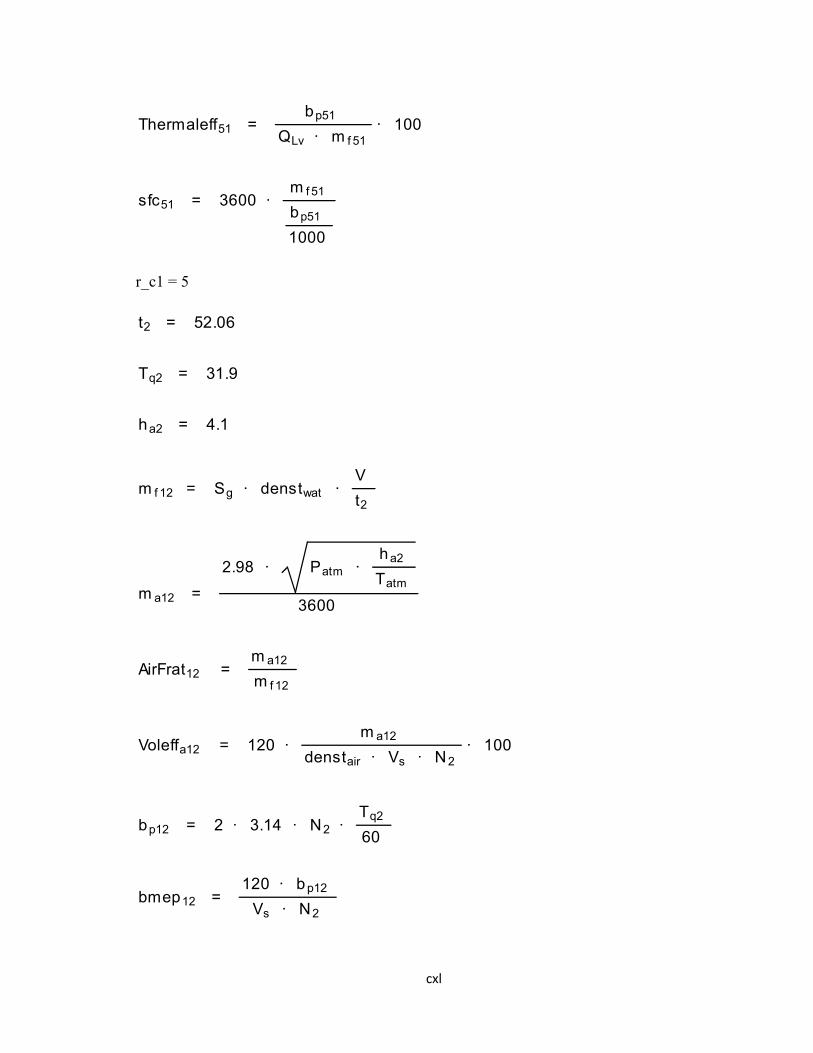
cxl
r_c1 = 5
Thermaleff51 =bp51
QLv · m f 51· 100
sfc51 = 3600 ·m f 51
bp51
1000
t2 = 52.06
Tq2 = 31.9
ha2 = 4.1
m f 12 = Sg · denstwat ·V
t2
m a12 =
2.98 · Patm ·ha2
Tatm
3600
AirFrat12 =m a12
m f 12
Voleffa12 = 120 ·m a12
denstair · Vs · N2· 100
bp12 = 2 · 3.14 · N2 ·Tq2
60
bmep12 =120 · bp12
Vs · N2
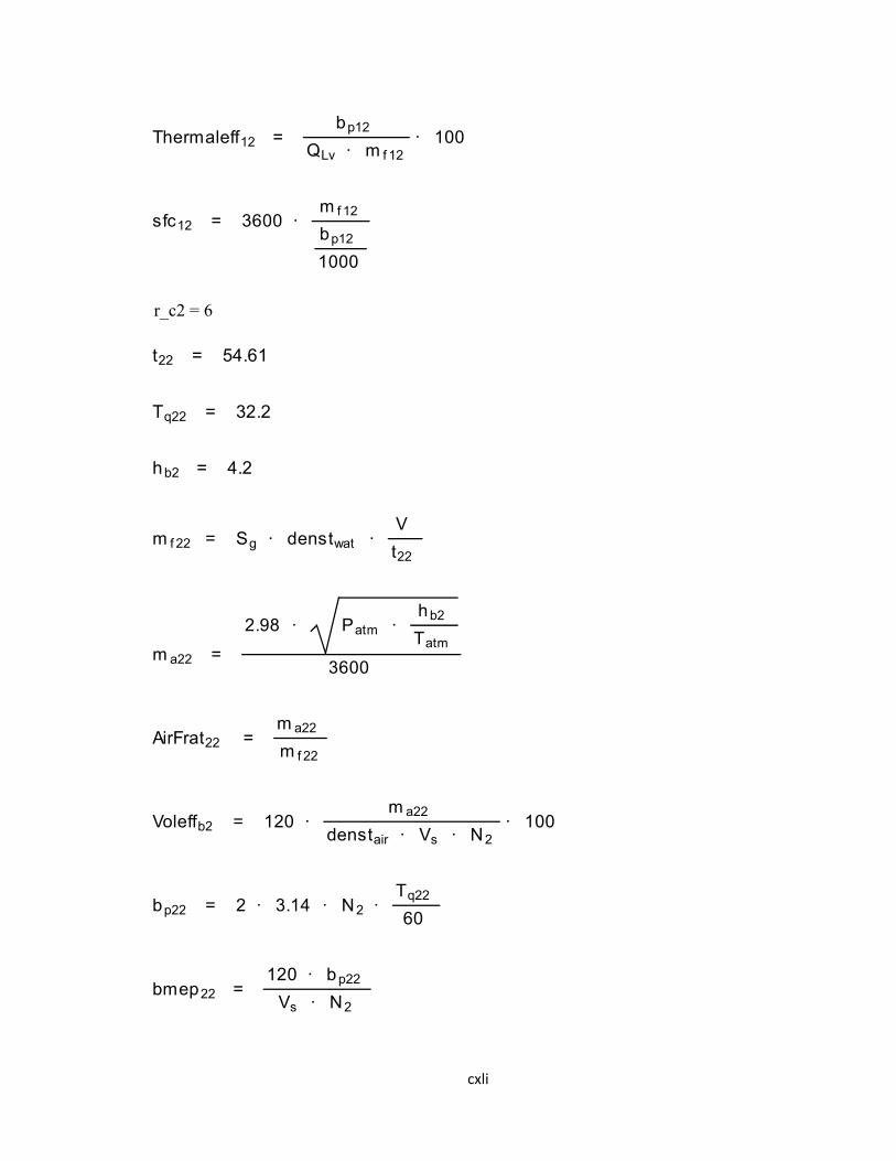
cxli
r_c2 = 6
Thermaleff12 =bp12
QLv · m f 12· 100
sfc12 = 3600 ·m f 12
bp12
1000
t22 = 54.61
Tq22 = 32.2
hb2 = 4.2
m f 22 = Sg · denstwat ·V
t22
m a22 =
2.98 · Patm ·hb2
Tatm
3600
AirFrat22 =m a22
m f 22
Voleffb2 = 120 ·m a22
denstair · Vs · N2· 100
bp22 = 2 · 3.14 · N2 ·Tq22
60
bmep22 =120 · bp22
Vs · N2

cxlii
r_c3 = 7
Thermaleff22 =bp22
QLv · m f 22· 100
sfc22 = 3600 ·m f 22
bp22
1000
t32 = 56.6
Tq32 = 32.9
hc2 = 4.2
m f 32 = Sg · denstwat ·V
t32
m a32 =
2.98 · Patm ·hc2
Tatm
3600
AirFrat32 =m a32
m f 32
Voleffc2 = 120 ·m a32
denstair · Vs · N2· 100
bp32 = 2 · 3.14 · N2 ·Tq32
60
bmep32 =120 · bp32
Vs · N2

cxliii
r_c4 = 8
Thermaleff32 =bp32
QLv · m f 32· 100
sfc32 = 3600 ·m f 32
bp32
1000
t42 = 59.89
Tq42 = 33
hd2 = 3.9
m f 42 = Sg · denstwat ·V
t42
m a42 =
2.98 · Patm ·hd2
Tatm
3600
AirFrat42 =m a42
m f 42
Voleffd2 = 120 ·m a42
denstair · Vs · N2· 100
bp42 = 2 · 3.14 · N2 ·Tq42
60
bmep42 =120 · bp42
Vs · N2

cxliv
r_c5 = 9
Thermaleff42 =bp42
QLv · m f 42· 100
sfc42 = 3600 ·m f 42
bp42
1000
t52 = 65.8
Tq52 = 33.1
he2 = 4.3
m f 52 = Sg · denstwat ·V
t52
m a52 =
2.98 · Patm ·he2
Tatm
3600
AirFrat52 =m a52
m f 52
Voleffe2 = 120 ·m a52
denstair · Vs · N2· 100
bp52 = 2 · 3.14 · N2 ·Tq52
60
bmep52 =120 · bp52
Vs · N2

cxlv
r_c1= 5
Thermaleff52 =bp52
QLv · m f 52· 100
sfc52 = 3600 ·m f 52
bp52
1000
t3 = 50.1
Tq3 = 31.5
ha3 = 4.7
m f 13 = Sg · denstwat ·V
t3
m a13 =
2.98 · Patm ·ha3
Tatm
3600
AirFrat13 =m a13
m f 13
Voleffa13 = 120 ·m a13
denstair · Vs · N3· 100
bp13 = 2 · 3.14 · N3 ·Tq3
60
bmep13 =120 · bp13
Vs · N3

cxlvi
r_c2 = 6
Thermaleff13 =bp13
QLv · m f 13· 100
sfc13 = 3600 ·m f 13
bp13
1000
t23 = 53.98
Tq23 = 32.1
hb3 = 4.9
m f 23 = Sg · denstwat ·V
t23
m a23 =
2.98 · Patm ·hb3
Tatm
3600
AirFrat23 =m a23
m f 23
Voleffb3 = 120 ·m a23
denstair · Vs · N3· 100
bp23 = 2 · 3.14 · N3 ·Tq23
60
bmep23 =120 · bp23
Vs · N3

cxlvii
r_c3 = 7
Thermaleff23 =bp23
QLv · m f 23· 100
sfc23 = 3600 ·m f 23
bp23
1000
t33 = 55.03
Tq33 = 32.2
hc3 = 4.9
m f 33 = Sg · denstwat ·V
t33
m a33 =
2.98 · Patm ·hc3
Tatm
3600
AirFrat33 =m a33
m f 33
Voleffc3 = 120 ·m a33
denstair · Vs · N3· 100
bp33 = 2 · 3.14 · N3 ·Tq33
60
bmep33 =120 · bp33
Vs · N3

cxlviii
r_c4 = 8
Thermaleff33 =bp33
QLv · m f 33· 100
sfc33 = 3600 ·m f 33
bp33
1000
t43 = 58.38
Tq43 = 32.9
hd3 = 4.9
m f 43 = Sg · denstwat ·V
t43
m a43 =
2.98 · Patm ·hd3
Tatm
3600
AirFrat43 =m a43
m f 43
Voleffd3 = 120 ·m a43
denstair · Vs · N3· 100
bp43 = 2 · 3.14 · N3 ·Tq43
60
bmep43 =120 · bp43
Vs · N3

cxlix
r_c5 = 9
Thermaleff43 =bp43
QLv · m f 43· 100
sfc43 = 3600 ·m f 43
bp43
1000
t53 = 64.1
Tq53 = 32.9
he3 = 5.5
m f 53 = Sg · denstwat ·V
t53
m a53 =
2.98 · Patm ·he3
Tatm
3600
AirFrat53 =m a53
m f 53
Voleffe3 = 120 ·m a53
denstair · Vs · N3· 100
bp53 = 2 · 3.14 · N3 ·Tq53
60
bmep53 =120 · bp53
Vs · N3
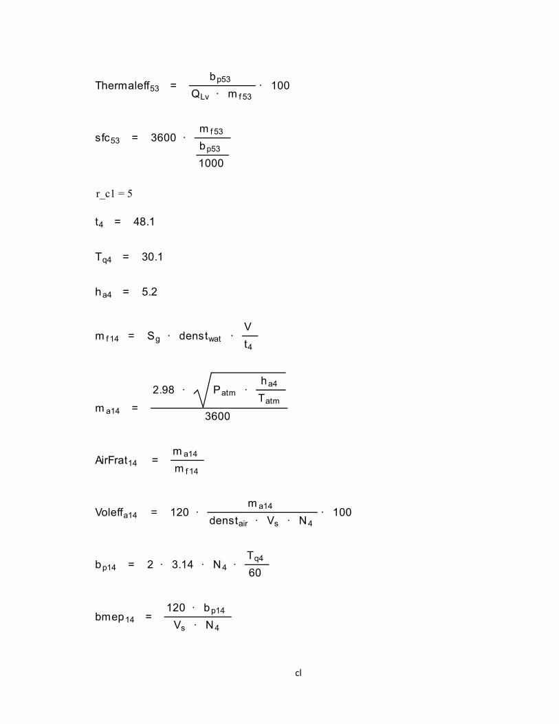
cl
r_c1 = 5
Thermaleff53 =bp53
QLv · m f 53· 100
sfc53 = 3600 ·m f 53
bp53
1000
t4 = 48.1
Tq4 = 30.1
ha4 = 5.2
m f 14 = Sg · denstwat ·V
t4
m a14 =
2.98 · Patm ·ha4
Tatm
3600
AirFrat14 =m a14
m f 14
Voleffa14 = 120 ·m a14
denstair · Vs · N4· 100
bp14 = 2 · 3.14 · N4 ·Tq4
60
bmep14 =120 · bp14
Vs · N4
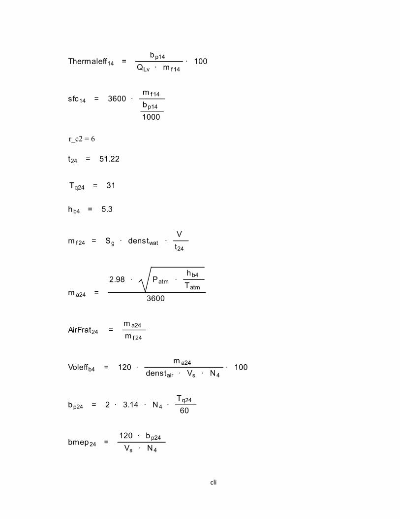
cli
r_c2 = 6
Thermaleff14 =bp14
QLv · m f 14· 100
sfc14 = 3600 ·m f 14
bp14
1000
t24 = 51.22
Tq24 = 31
hb4 = 5.3
m f 24 = Sg · denstwat ·V
t24
m a24 =
2.98 · Patm ·hb4
Tatm
3600
AirFrat24 =m a24
m f 24
Voleffb4 = 120 ·m a24
denstair · Vs · N4· 100
bp24 = 2 · 3.14 · N4 ·Tq24
60
bmep24 =120 · bp24
Vs · N4

clii
r_c3 = 7
Thermaleff24 =bp24
QLv · m f 24· 100
sfc24 = 3600 ·m f 24
bp24
1000
t34 = 53.9
Tq34 = 31.5
hc4 = 5.3
m f 34 = Sg · denstwat ·V
t34
m a34 =
2.98 · Patm ·hc4
Tatm
3600
AirFrat34 =m a34
m f 34
Voleffc4 = 120 ·m a34
denstair · Vs · N4· 100
bp34 = 2 · 3.14 · N4 ·Tq34
60
bmep34 =120 · bp34
Vs · N4

cliii
r_c4 = 8
Thermaleff34 =bp34
QLv · m f 34· 100
sfc34 = 3600 ·m f 34
bp34
1000
t44 = 58.22
Tq44 = 31.6
hd4 = 5.5
m f 44 = Sg · denstwat ·V
t44
m a44 =
2.98 · Patm ·hd4
Tatm
3600
AirFrat44 =m a44
m f 44
Voleffd4 = 120 ·m a44
denstair · Vs · N4· 100
bp44 = 2 · 3.14 · N4 ·Tq44
60
bmep44 =120 · bp44
Vs · N4

cliv
r_c5 = 9
Thermaleff44 =bp44
QLv · m f 44· 100
sfc44 = 3600 ·m f 44
bp44
1000
t54 = 62.8
Tq54 = 31.7
he4 = 5.7
m f 54 = Sg · denstwat ·V
t54
m a54 =
2.98 · Patm ·he4
Tatm
3600
AirFrat54 =m a54
m f 54
Voleffe4 = 120 ·m a54
denstair · Vs · N4· 100
bp54 = 2 · 3.14 · N4 ·Tq54
60
bmep54 =120 · bp54
Vs · N4

clv
r_c1 = 5
Thermaleff54 =bp54
QLv · m f 54· 100
sfc54 = 3600 ·m f 54
bp54
1000
t5 = 44.5
Tq5 = 28.9
ha5 = 5.5
m f 15 = Sg · denstwat ·V
t5
m a15 =
2.98 · Patm ·ha5
Tatm
3600
AirFrat15 =m a15
m f 15
Voleffa15 = 120 ·m a15
denstair · Vs · N5· 100
bp15 = 2 · 3.14 · N5 ·Tq5
60
bmep15 =120 · bp15
Vs · N5
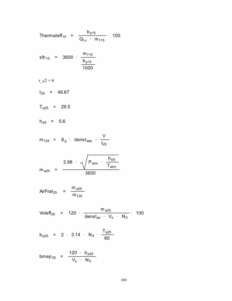
clvi
r_c2 = 6
Thermaleff15 =bp15
QLv · m f 15· 100
sfc15 = 3600 ·m f 15
bp15
1000
t25 = 48.67
Tq25 = 29.5
hb5 = 5.6
m f 25 = Sg · denstwat ·V
t25
m a25 =
2.98 · Patm ·hb5
Tatm
3600
AirFrat25 =m a25
m f 25
Voleffb5 = 120 ·m a25
denstair · Vs · N5· 100
bp25 = 2 · 3.14 · N5 ·Tq25
60
bmep25 =120 · bp25
Vs · N5

clvii
r_c = 3 = 7
Thermaleff25 =bp25
QLv · m f 25· 100
sfc25 = 3600 ·m f 25
bp25
1000
t35 = 50.13
Tq35 = 30.1
hc5 = 5.8
m f 35 = Sg · denstwat ·V
t35
m a35 =
2.98 · Patm ·hc5
Tatm
3600
AirFrat35 =m a35
m f 35
Voleffc5 = 120 ·m a35
denstair · Vs · N5· 100
bp35 = 2 · 3.14 · N5 ·Tq35
60
bmep35 =120 · bp35
Vs · N5

clviii
r_c4 = 8
Thermaleff35 =bp35
QLv · m f 35· 100
sfc35 = 3600 ·m f 35
bp35
1000
t45 = 53.6
Tq45 = 30.5
hd5 = 6
m f 45 = Sg · denstwat ·V
t45
m a45 =
2.98 · Patm ·hd5
Tatm
3600
AirFrat45 =m a45
m f 45
Voleffd5 = 120 ·m a45
denstair · Vs · N5· 100
bp45 = 2 · 3.14 · N5 ·Tq45
60
bmep45 =120 · bp45
Vs · N5

clix
r_c5 = 9
Thermaleff45 =bp45
QLv · m f 45· 100
sfc45 = 3600 ·m f 45
bp45
1000
t55 = 61.2
Tq55 = 30.7
he5 = 6.1
m f 55 = Sg · denstwat ·V
t55
m a55 =
2.98 · Patm ·he5
Tatm
3600
AirFrat55 =m a55
m f 55
Voleffe5 = 120 ·m a55
denstair · Vs · N5· 100
bp55 = 2 · 3.14 · N5 ·Tq55
60
bmep55 =120 · bp55
Vs · N5

clx
r_c1 = 5
Thermaleff55 =bp55
QLv · m f 55· 100
sfc55 = 3600 ·m f 55
bp55
1000
t6 = 40.3
Tq6 = 27.4
ha6 = 5.7
m f 16 = Sg · denstwat ·V
t6
m a16 =
2.98 · Patm ·ha6
Tatm
3600
AirFrat16 =m a16
m f 16
Voleffa16 = 120 ·m a16
denstair · Vs · N6· 100
bp16 = 2 · 3.14 · N6 ·Tq6
60
bmep16 =120 · bp16
Vs · N6

clxi
r_c2 = 6
Thermaleff16 =bp16
QLv · m f 16· 100
sfc16 = 3600 ·m f 16
bp16
1000
t26 = 45.2
Tq26 = 27.9
hb6 = 5.9
m f 26 = Sg · denstwat ·V
t26
m a26 =
2.98 · Patm ·hb6
Tatm
3600
AirFrat26 =m a26
m f 26
Voleffb6 = 120 ·m a26
denstair · Vs · N6· 100
bp26 = 2 · 3.14 · N6 ·Tq26
60
bmep26 =120 · bp26
Vs · N6

clxii
r_c3 = 7
Thermaleff26 =bp26
QLv · m f 26· 100
sfc26 = 3600 ·m f 26
bp26
1000
t36 = 46.5
Tq36 = 28.4
hc6 = 6.1
m f 36 = Sg · denstwat ·V
t36
m a36 =
2.98 · Patm ·hc6
Tatm
3600
AirFrat36 =m a36
m f 36
Voleffc6 = 120 ·m a36
denstair · Vs · N6· 100
bp36 = 2 · 3.14 · N6 ·Tq36
60
bmep36 =120 · bp36
Vs · N6

clxiii
r_c4 = 8
Thermaleff36 =bp36
QLv · m f 36· 100
sfc36 = 3600 ·m f 36
bp36
1000
t46 = 52.2
Tq46 = 28.6
hd6 = 6.2
m f 46 = Sg · denstwat ·V
t46
m a46 =
2.98 · Patm ·hd6
Tatm
3600
AirFrat46 =m a46
m f 46
Voleffd6 = 120 ·m a46
denstair · Vs · N6· 100
bp46 = 2 · 3.14 · N6 ·Tq46
60
bmep46 =120 · bp46
Vs · N6

clxiv
r_c5 = 9
Thermaleff46 =bp46
QLv · m f 46· 100
sfc46 = 3600 ·m f 46
bp46
1000
t56 = 58.8
Tq56 = 29.1
he6 = 6.6
m f 56 = Sg · denstwat ·V
t56
m a56 =
2.98 · Patm ·he6
Tatm
3600
AirFrat56 =m a56
m f 56
Voleffe6 = 120 ·m a56
denstair · Vs · N6· 100
bp56 = 2 · 3.14 · N6 ·Tq56
60
bmep56 =120 · bp56
Vs · N6
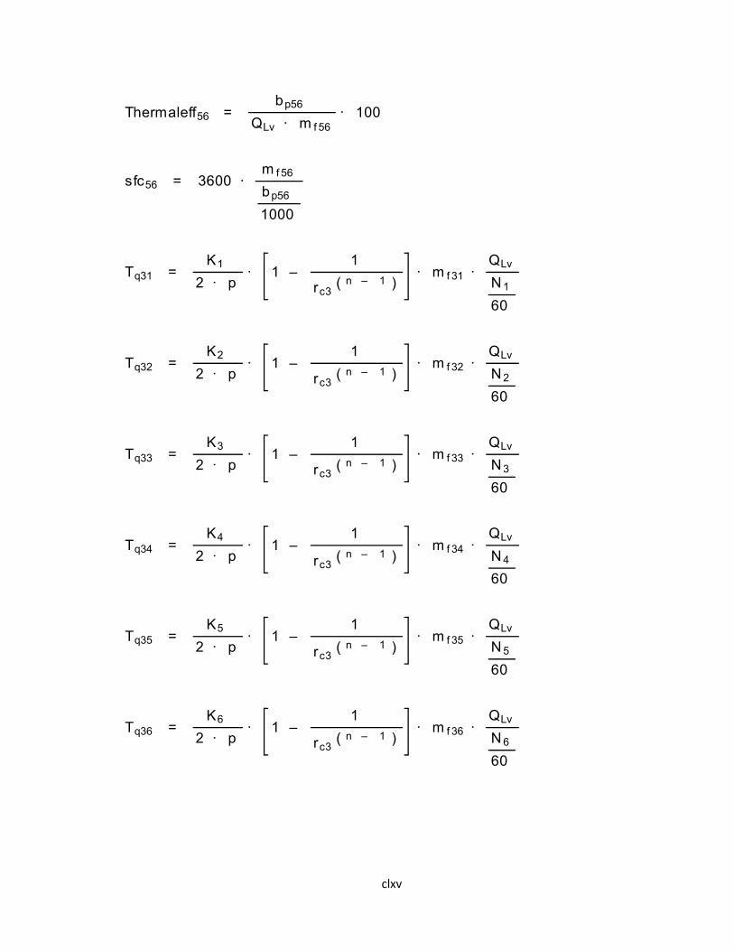
clxv
Thermaleff56 =bp56
QLv · m f 56· 100
sfc56 = 3600 ·m f 56
bp56
1000
Tq31 =K1
2 · p· 1 –
1
rc3( n – 1 )
· m f 31 ·QLv
N1
60
Tq32 =K2
2 · p· 1 –
1
rc3( n – 1 )
· m f 32 ·QLv
N2
60
Tq33 =K3
2 · p· 1 –
1
rc3( n – 1 )
· m f 33 ·QLv
N3
60
Tq34 =K4
2 · p· 1 –
1
rc3( n – 1 )
· m f 34 ·QLv
N4
60
Tq35 =K5
2 · p· 1 –
1
rc3( n – 1 )
· m f 35 ·QLv
N5
60
Tq36 =K6
2 · p· 1 –
1
rc3( n – 1 )
· m f 36 ·QLv
N6
60
clxvi
APPENDIX D
[Formatted equations for theoretical analysis]
r_c1 = 5
Tq1 = 32.6
Tq2 = 32.9
Tq3 = 32.2
Tq4 = 31.5
Tq6 = 28.4
Tq11 = Tq1 – ( 5 / 7 )0.4
Bp11 = 2 · 3.14 · N1 ·Tq11
60
clxvii
r_c2 = 6
r_c3 = 8
Tq11 =K1
2 · 3.14· 1 –
1
50.4
· 60 · m f 11 ·QLv
N1
BMEP11 = 120 ·Bp11
Vs · N1
THERMALEFF11 =Bp11
QLv · m f 11
SFC11 = 3600 ·m f 11
Bp11
1000
Tq21 = Tq1 – ( 6 / 7 )0.4
Bp21 = 2 · 3.14 · N1 ·Tq21
60
Tq21 =K1
2 · 3.14· 1 –
1
6 0.4· 60 · m f 21 ·
QLv
N 1
BMEP21 = 120 ·Bp21
Vs · N1
THERMALEFF21 =Bp21
QLv · m f 21
SFC21 = 3600 ·m f 21
Bp21
1000

clxviii
r_c4 = 9
Tq31 = Tq1 + ( 8 / 7 )0.4
Bp31 = 2 · 3.14 · N1 ·Tq31
60
Tq31 =K1
2 · 3.14· 1 –
1
8 0.4· 60 · m f 31 ·
QLv
N 1
BMEP31 = 120 ·Bp31
Vs · N1
THERMALEFF31 =Bp31
QLv · m f 31
SFC31 = 3600 ·m f 31
Bp31
1000
Tq41 = Tq1 + ( 9 / 7 )0.4
Bp41 = 2 · 3.14 · N1 ·Tq41
60
Tq41 =K1
2 · 3.14· 1 –
1
9 0.4· 60 · m f 41 ·
QLv
N 1
BMEP41 = 120 ·Bp41
Vs · N1
THERMALEFF41 =Bp41
QLv · m f 41

clxix
r_c5 = 7
r_c1 = 5
SFC41 = 3600 ·m f 41
Bp41
1000
Bp51 =Bp31 + Bp21
2
Tq51 =Tq31 + Tq21
2
m f 51 =m f 31 + m f 21
2
BMEP51 =BMEP31 + BMEP21
2
THERMALEFF51 =THERMALEFF31 + THERMALEFF21
2
SFC51 =SFC31 + SFC21
2
Tq12 = Tq2 – ( 5 / 7 )0.4
Bp12 = 2 · 3.14 · N2 ·Tq12
60
Tq12 =K2
2 · 3.14· 1 –
1
5 0.4· 60 · m f 12 ·
QLv
N 2

clxx
r_c2 = 6
r_c3 = 8
BMEP12 = 120 ·Bp12
Vs · N2
THERMALEFF12 =Bp12
QLv · m f 12
SFC12 = 3600 ·m f 12
Bp12
1000
Tq22 = Tq2 – ( 6 / 7 )0.4
Bp22 = 2 · 3.14 · N2 ·Tq22
60
Tq22 =K2
2 · 3.14· 1 –
1
60.4
· 60 · m f 22 ·QLv
N2
BMEP22 = 120 ·Bp22
Vs · N2
THERMALEFF22 =Bp22
QLv · m f 22
SFC22 = 3600 ·m f 22
Bp22
1000

clxxi
r_c4 = 9
Tq32 = Tq2 + ( 8 / 7 )0.4
Bp32 = 2 · 3.14 · N2 ·Tq32
60
Tq32 =K2
2 · 3.14· 1 –
1
8 0.4· 60 · m f 32 ·
QLv
N 2
BMEP32 = 120 ·Bp32
Vs · N2
THERMALEFF32 =Bp32
QLv · m f 32
SFC32 = 3600 ·m f 32
Bp32
1000
Tq42 = Tq2 + ( 9 / 7 )0.4
Bp42 = 2 · 3.14 · N2 ·Tq42
60
Tq42 =K2
2 · 3.14· 1 –
1
9 0.4· 60 · m f 42 ·
QLv
N 2
BMEP42 = 120 ·Bp42
Vs · N2
THERMALEFF42 =Bp42
QLv · m f 42

clxxii
r_c5 = 7
r_c1 = 5
SFC42 = 3600 ·m f 42
Bp42
1000
Bp52 =Bp32 + Bp22
2
Tq52 =Tq32 + Tq22
2
m f 52 =m f 32 + m f 22
2
BMEP52 =BMEP32 + BMEP22
2
THERMALEFF52 =THERMALEFF32 + THERMALEFF22
2
SFC52 =SFC32 + SFC22
2
Tq13 = Tq3 – ( 5 / 7 )0.4
Bp13 = 2 · 3.14 · N3 ·Tq13
60
Tq13 =K3
2 · 3.14· 1 –
1
5 0.4· 60 · m f 13 ·
QLv
N 3
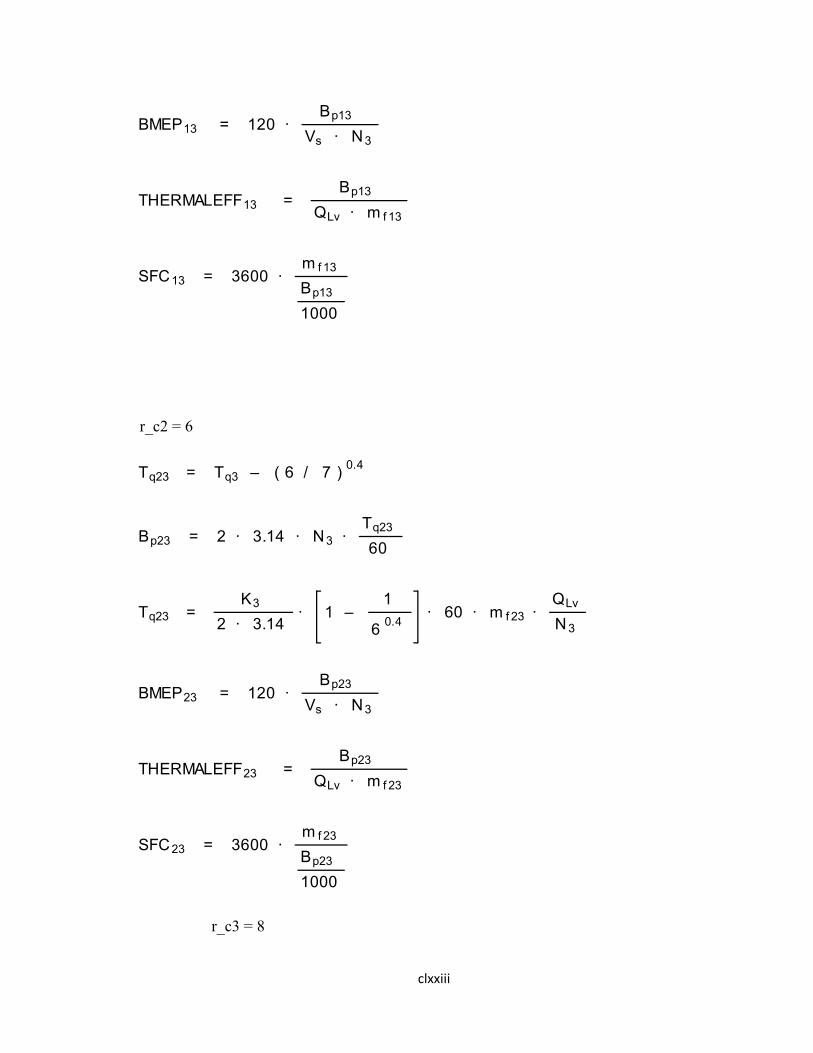
clxxiii
r_c2 = 6
r_c3 = 8
BMEP13 = 120 ·Bp13
Vs · N3
THERMALEFF13 =Bp13
QLv · m f 13
SFC13 = 3600 ·m f 13
Bp13
1000
Tq23 = Tq3 – ( 6 / 7 )0.4
Bp23 = 2 · 3.14 · N3 ·Tq23
60
Tq23 =K3
2 · 3.14· 1 –
1
60.4
· 60 · m f 23 ·QLv
N3
BMEP23 = 120 ·Bp23
Vs · N3
THERMALEFF23 =Bp23
QLv · m f 23
SFC23 = 3600 ·m f 23
Bp23
1000

clxxiv
r_c4 = 9
Tq33 = Tq3 + ( 8 / 7 )0.4
Bp33 = 2 · 3.14 · N3 ·Tq33
60
Tq33 =K3
2 · 3.14· 1 –
1
8 0.4· 60 · m f 33 ·
QLv
N 3
BMEP33 = 120 ·Bp33
Vs · N3
THERMALEFF33 =Bp33
QLv · m f 33
SFC33 = 3600 ·m f 33
Bp33
1000
Tq43 = Tq3 + ( 9 / 7 )0.4
Bp43 = 2 · 3.14 · N3 ·Tq43
60
Tq43 =K3
2 · 3.14· 1 –
1
9 0.4· 60 · m f 43 ·
QLv
N 3
BMEP43 = 120 ·Bp43
Vs · N3
THERMALEFF43 =Bp43
QLv · m f 43

clxxv
r_c5 = 7
r_c1 = 5
SFC43 = 3600 ·m f 43
Bp43
1000
Bp53 =Bp33 + Bp23
2
Tq53 =Tq33 + Tq23
2
m f 53 =m f 33 + m f 23
2
BMEP53 =BMEP33 + BMEP23
2
THERMALEFF53 =THERMALEFF33 + THERMALEFF23
2
SFC53 =SFC33 + SFC23
2
Tq14 = Tq4 – ( 5 / 7 )0.4
Bp14 = 2 · 3.14 · N4 ·Tq14
60
Tq14 =K4
2 · 3.14· 1 –
1
5 0.4· 60 · m f 14 ·
QLv
N 4

clxxvi
r_c2 = 6
r_c3 = 8
BMEP14 = 120 ·Bp14
Vs · N4
THERMALEFF14 =Bp14
QLv · m f 14
SFC14 = 3600 ·m f 14
Bp14
1000
Tq24 = Tq4 – ( 6 / 7 )0.4
Bp24 = 2 · 3.14 · N4 ·Tq24
60
Tq24 =K4
2 · 3.14· 1 –
1
60.4
· 60 · m f 24 ·QLv
N4
BMEP24 = 120 ·Bp24
Vs · N4
THERMALEFF24 =Bp24
QLv · m f 24
SFC24 = 3600 ·m f 24
Bp24
1000
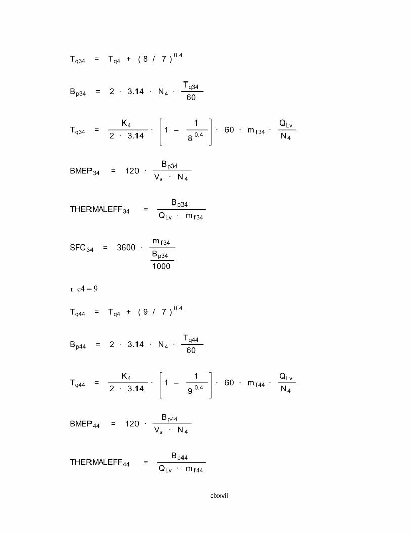
clxxvii
r_c4 = 9
Tq34 = Tq4 + ( 8 / 7 )0.4
Bp34 = 2 · 3.14 · N4 ·Tq34
60
Tq34 =K4
2 · 3.14· 1 –
1
8 0.4· 60 · m f 34 ·
QLv
N 4
BMEP34 = 120 ·Bp34
Vs · N4
THERMALEFF34 =Bp34
QLv · m f 34
SFC34 = 3600 ·m f 34
Bp34
1000
Tq44 = Tq4 + ( 9 / 7 )0.4
Bp44 = 2 · 3.14 · N4 ·Tq44
60
Tq44 =K4
2 · 3.14· 1 –
1
9 0.4· 60 · m f 44 ·
QLv
N 4
BMEP44 = 120 ·Bp44
Vs · N4
THERMALEFF44 =Bp44
QLv · m f 44
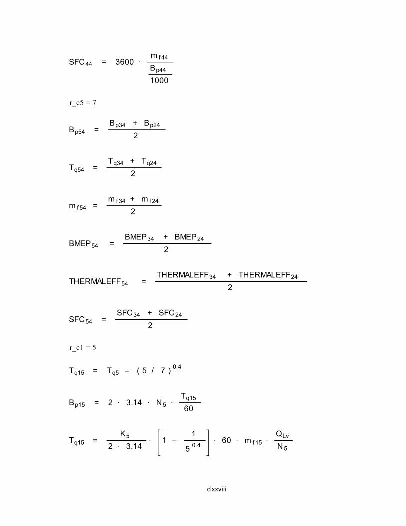
clxxviii
r_c5 = 7
r_c1 = 5
SFC44 = 3600 ·m f 44
Bp44
1000
Bp54 =Bp34 + Bp24
2
Tq54 =Tq34 + Tq24
2
m f 54 =m f 34 + m f 24
2
BMEP54 =BMEP34 + BMEP24
2
THERMALEFF54 =THERMALEFF34 + THERMALEFF24
2
SFC54 =SFC34 + SFC24
2
Tq15 = Tq5 – ( 5 / 7 )0.4
Bp15 = 2 · 3.14 · N5 ·Tq15
60
Tq15 =K5
2 · 3.14· 1 –
1
5 0.4· 60 · m f 15 ·
QLv
N 5

clxxix
r_c2 = 6
r_c3 = 8
BMEP15 = 120 ·Bp15
Vs · N5
THERMALEFF15 =Bp15
QLv · m f 15
SFC15 = 3600 ·m f 15
Bp15
1000
Tq25 = Tq5 – ( 6 / 7 )0.4
Bp25 = 2 · 3.14 · N5 ·Tq25
60
Tq25 =K5
2 · 3.14· 1 –
1
60.4
· 60 · m f 25 ·QLv
N5
BMEP25 = 120 ·Bp25
Vs · N5
THERMALEFF25 =Bp25
QLv · m f 25
SFC25 = 3600 ·m f 25
Bp25
1000

clxxx
r_c4 = 9
Tq35 = Tq5 + ( 8 / 7 )0.4
Bp35 = 2 · 3.14 · N5 ·Tq35
60
Tq35 =K5
2 · 3.14· 1 –
1
8 0.4· 60 · m f 35 ·
QLv
N 5
BMEP35 = 120 ·Bp35
Vs · N5
THERMALEFF35 =Bp35
QLv · m f 35
SFC35 = 3600 ·m f 35
Bp35
1000
Tq45 = Tq5 + ( 9 / 7 )0.4
Bp45 = 2 · 3.14 · N5 ·Tq45
60
Tq45 =K5
2 · 3.14· 1 –
1
9 0.4· 60 · m f 45 ·
QLv
N 5
BMEP45 = 120 ·Bp45
Vs · N5
THERMALEFF45 =Bp45
QLv · m f 45

clxxxi
r_c5 = 7
r_c1 = 5
SFC45 = 3600 ·m f 45
Bp45
1000
Bp55 =Bp35 + Bp25
2
Tq55 =Tq35 + Tq25
2
m f 55 =m f 35 + m f 25
2
BMEP55 =BMEP35 + BMEP25
2
THERMALEFF55 =THERMALEFF35 + THERMALEFF25
2
SFC55 =SFC35 + SFC25
2
Tq16 = Tq6 – ( 5 / 7 )0.4
Bp16 = 2 · 3.14 · N6 ·Tq16
60
Tq16 =K6
2 · 3.14· 1 –
1
5 0.4· 60 · m f 16 ·
QLv
N 6
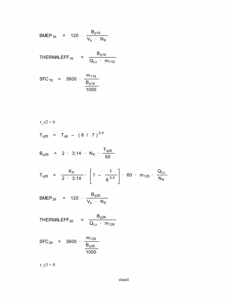
clxxxii
r_c2 = 6
r_c3 = 8
BMEP16 = 120 ·Bp16
Vs · N6
THERMALEFF16 =Bp16
QLv · m f 16
SFC16 = 3600 ·m f 16
Bp16
1000
Tq26 = Tq6 – ( 6 / 7 )0.4
Bp26 = 2 · 3.14 · N6 ·Tq26
60
Tq26 =K6
2 · 3.14· 1 –
1
60.4
· 60 · m f 26 ·QLv
N6
BMEP26 = 120 ·Bp26
Vs · N6
THERMALEFF26 =Bp26
QLv · m f 26
SFC26 = 3600 ·m f 26
Bp26
1000

clxxxiii
r_c4 = 9
Tq36 = Tq6 + ( 8 / 7 )0.4
Bp36 = 2 · 3.14 · N6 ·Tq36
60
Tq36 =K6
2 · 3.14· 1 –
1
8 0.4· 60 · m f 36 ·
QLv
N 6
BMEP36 = 120 ·Bp36
Vs · N6
THERMALEFF36 =Bp36
QLv · m f 36
SFC36 = 3600 ·m f 36
Bp36
1000
Tq46 = Tq6 + ( 9 / 7 )0.4
Bp46 = 2 · 3.14 · N6 ·Tq46
60
Tq46 =K6
2 · 3.14· 1 –
1
9 0.4· 60 · m f 46 ·
QLv
N 6
BMEP46 = 120 ·Bp46
Vs · N6
THERMALEFF46 =Bp46
QLv · m f 46
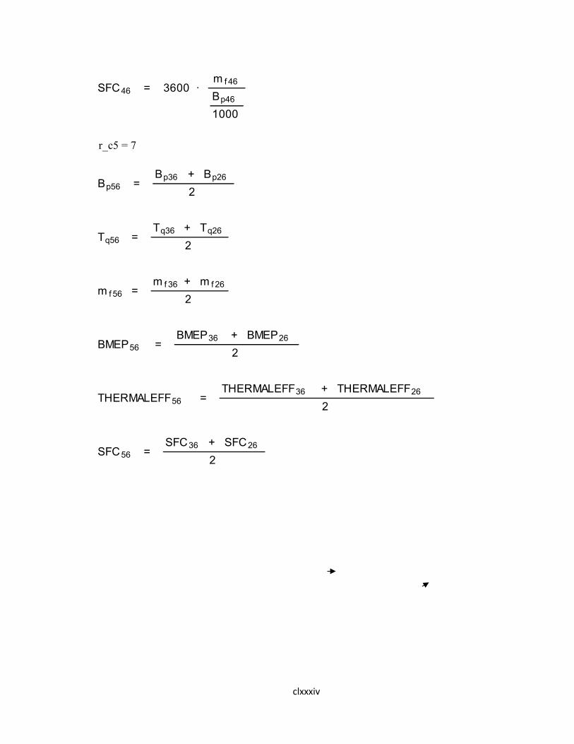
clxxxiv
r_c5 = 7
SFC46 = 3600 ·m f 46
Bp46
1000
Bp56 =Bp36 + Bp26
2
Tq56 =Tq36 + Tq26
2
m f 56 =m f 36 + m f 26
2
BMEP56 =BMEP36 + BMEP26
2
THERMALEFF56 =THERMALEFF36 + THERMALEFF26
2
SFC56 =SFC36 + SFC26
2
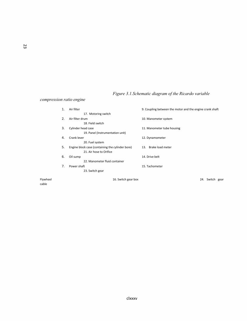
clxxxv
Figure 3.1.Schematic diagram of the Ricardo variable compression ratio engine
1. Air filter 9. Coupling between the motor and the engine crank shaft17. Motoring switch
2. Air filter drum 10. Manometer system18. Field switch
3. Cylinder head case 11. Manometer tube housing19. Panel (Instrumentation unit)
4. Crank lever 12. Dynamometer20. Fuel system
5. Engine block case (containing the cylinder bore) 13. Brake load meter21. Air hose to Orifice
6. Oil sump 14. Drive belt22. Manometer fluid container
7. Power shaft 15. Tachometer23. Switch gear
Flywheel 16. Switch gear box 24. Switch gear cable
23