Understanding India's Food Inflation: The Role of Demand and ...

Inflation, the Payments Period, and the Demand for
Money
(Article begins on next page)
The Harvard community has made this article openlyavailable.
Please share how this access benefits you. Your storymatters.
Citation Barro, Robert J. 1970. Inflation, the payments period, and thedemand for money. Journal of Political Economy 78(6):1228-1263.
Published Version doi:10.1086/259707
Accessed August 21, 2018 6:07:33 PM EDT
Citable Link http://nrs.harvard.edu/urn-3:HUL.InstRepos:3451392
Terms of Use This article was downloaded from Harvard University'sDASH repository, and is made available under the terms andconditions applicable to Other Posted Material, as set forth athttp://nrs.harvard.edu/urn-3:HUL.InstRepos:dash.current.terms-of-use#LAA

Inflation, the Payments Period, and the Demand for Money
Robert J. Barro Brown University
Part I of this paper develops a model of economic response to inflation. Sections A, B, and C consider the maximizing behavior of employers and employees in the context of a steady rate of inflation. Since the rate of price change can be translated into an effective cost of holding money, a higher rate provides increased incentive for economizing on cash balances. Two methods of economizing are considered: first, (Sections A and B), reductions of the time interval between various types of payments (increases in "velocity") and, second (Section C), decreases in the fraction of "monetized" transactions.
With a given fraction of monetized transactions, the selection of the optimal length of time between (wage and other types of) payments involves a tradeoff of the inventory type. Given some fixed (real) cost of making payments, a higher rate of price change reduces the optimal- payment interval (increases velocity) and produces a corresponding reduction in average real money holdings.
The demand-for-money function which is implied by optimal-payments period selection approaches an inflation-rate elasticity of - 1/2 as the rate of inflation becomes large (relative to real rates of return in the economy). However, this formulation assumes that the fraction of monetized trans- actions is unaffected by changes in the inflation rate. In fact, "money" may be viewed as a medium which provides certain transactions benefits (in terms of physical convenience, general acceptability, et cetera) in comparison with alternative media. At a higher rate of price change, the cost of retaining money as a payments medium is increased (relative to
The author is grateful for helpful comments from Zvi Griliches, Michael Connolly, Gary Becker, Milton Friedman, Herschel Grossman, and Marc Nerlove. This paper is a portion of the author's Ph.D. thesis at Harvard University.-
1228
INFLATION AND DEMAND FOR MONEY 1229
that for stable-valued substitutes, such as payments in kind or foreign exchange). If this inflationary cost is weighed against money's trans- actions benefits, the fraction of expenditures for which it pays to retain money is inversely related to the rate of price change. The combination of this money-substitute effect with the previously described velocity mechanism produces an increasing (absolute) elasticity of money demand to the rate of inflation.
The analysis of Sections A, B, and C assumes a constant rate of price change. Section D extends the analysis to consider the optimal response to rates of inflation which vary over time. Basically, if no costs of adjust- ment or lags in perception are involved, the steady-state solution would be optimal at all times. Accordingly, if lags in perception are neglected, the optimal response to changing rates of inflation involves a weighing of adjustment costs (for example, costs of instituting changes in the pay- ments period) against "out-of-equilibrium" costs (that is, costs of not adhering to the steady-state rules at all times). The model of Section D assumes that actual rates of price change are generated by a symmetric, stochastic process (a random walk), and that individuals adopt an adjust- ment policy of the (S, s) inventory form. According to this type of policy, variations in the inflation rate produce no response (in, say, the payments period or the fraction of monetized transactions) until some critical gap between actual and statically optimal levels appears. At this point some discrete adjustment of decision variables is performed in accordance with the optimal steady-state relationships. No subsequent adjustments occur until a new gap of the critical size appears,
The (S, s) response model is used to obtain an aggregate mechanism for generating "effective" rates of inflation (the rate which is relevant for key decision variables, and, therefore, for demand for money). The mecha- nism is similar in form to earlier models of the adaptive-expectations type (Cagan 1956), although the current model reflects solely an adjustment lag. A key implication of maximizing behavior is the dependence of the re- sponse coefficient on the (effective) rate of inflation itself.
The theory of Part I is applied in Part II to an empirical study of demand for money. The data derive from four cases of post-World War I hyper- inflation (Austria, Germany, Hungary, and Poland), which were previously studied by Cagan (1956) and Allais (1966). Substantial space is devoted to constructing null hypotheses which embody the theoretical implications of Part I. Basically, these null hypotheses involve a priori conjectures on the coefficients of regression equations. The (nonlinear, iterative) empirical estimation and testing confirms the bulk of these conjectures, and, there- fore, provides support for the underlying theory. Comments on the statis- tical results and avenues for future research are indicated at the end of the paper.
1230 JOURNAL OF POLITICAL ECONOMY
1. A Model of the Payments Period and the Demand for Money
A. The Basic Steady-State Model
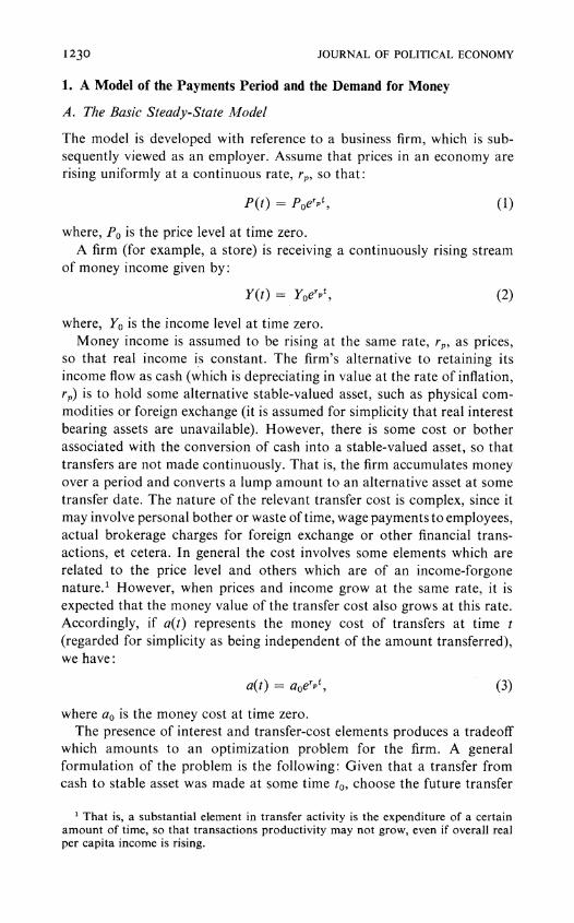
The model is developed with reference to a business firm, which is sub- sequently viewed as an employer. Assume that prices in an economy are rising uniformly at a continuous rate, rp, so that:
P(t) = Poervt, (1)
where, PO is the price level at time zero. A firm (for example, a store) is receiving a continuously rising stream
of money income given by:
Y(t)= Yoerpt, (2)
where, YO is the income level at time zero. Money income is assumed to be rising at the same rate, rp, as prices,
so that real income is constant. The firm's alternative to retaining its income flow as cash (which is depreciating in value at the rate of inflation, rp) is to hold some alternative stable-valued asset, such as physical com- modities or foreign exchange (it is assumed for simplicity that real interest bearing assets are unavailable). However, there is some cost or bother associated with the conversion of cash into a stable-valued asset, so that transfers are not made continuously. That is, the firm accumulates money over a period and converts a lump amount to an alternative asset at some transfer date. The nature of the relevant transfer cost is complex, since it may involve personal bother or waste of time, wage payments to employees, actual brokerage charges for foreign exchange or other financial trans- actions, et cetera. In general the cost involves some elements which are related to the price level and others which are of an income-forgone nature.' However, when prices and income grow at the same rate, it is expected that the money value of the transfer cost also grows at this rate. Accordingly, if a(t) represents the money cost of transfers at time t (regarded for simplicity as being independent of the amount transferred), we have:
a(t) = aoerpt, (3)
where ao is the money cost at time zero. The presence of interest and transfer-cost elements produces a tradeoff
which amounts to an optimization problem for the firm. A general formulation of the problem is the following: Given that a transfer from cash to stable asset was made at some time to, choose the future transfer
1 That is, a substantial element in transfer activity is the expenditure of a certain amount of time, so that transactions productivity may not grow, even if overall real per capita income is rising.
INFLATION AND DEMAND FOR MONEY I231
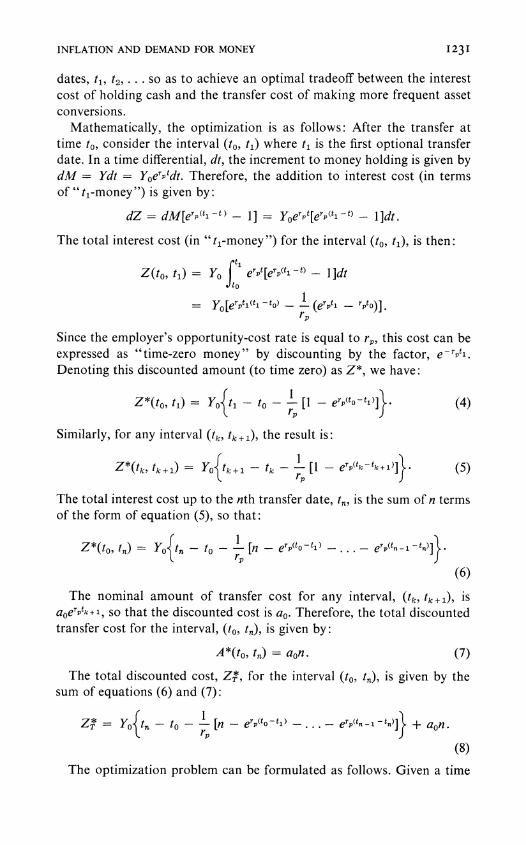
dates, t1, t2, . . . so as to achieve an optimal tradeoff between the interest cost of holding cash and the transfer cost of making more frequent asset conversions.
Mathematically, the optimization -is as follows: After the transfer at time to, consider the interval (to, t1) where t1 is the first optional transfer date. In a time differential, dt, the increment to money holding is given by dM = Ydt = Yoerptdt. Therefore, the addition to interest cost (in terms of "t1-money") is given by:
dZ = dM[erp(tl -t)- 1] = yoerpt[erp(ti t) - I]dt.
The total interest cost (in " t1-money ") for the interval (to, t1), is then:
rti Z(to, t1) = Yo erPt[erp(ti -t) - 1]dt
= Yo [erpti (ti - to) - - (erpt, - rpto)]
Since the employer's opportunity-cost rate is equal to rp, this cost can be expressed as "time-zero money" by discounting by the factor, e-rptl.
Denoting this discounted amount (to time zero) as Z*, we have:
Z*(to, t1) = Yoti- to- I
[1 -erPfto l]-j (4)
Similarly, for any interval (tk, tk + 1), the result is:
Z*(tk, tk+1) = YO{tk + I - tk - I
[1 - erp(tk tk + 1]}. (5)
The total interest cost up to the nth transfer date, tn, is the sum of n terms of the form of equation (5), so that:
Z*(to, tn) = Yo tn - to - I
[n - erp(to-t1_ erP(tn -W
(6)
The nominal amount of transfer cost for any interval, (tk, tk + 1), is aoerptk + 1 so that the discounted cost is ao. Therefore, the total discounted transfer cost for the interval, (to, t), is given by:
A*(to, tn) = aon. (7)
The total discounted cost, ZT, for the interval (to, tn), is given by the sum of equations (6) and (7):
T= Yo{t, - to -0 I
rPtto ti) er ( tn)]} + aon.
(8)
The optimization problem can be formulated as follows. Given a time

I232 JOURNAL OF POLITICAL ECONOMY
interval, T= t, - to, with the constraint that the final transfer be made at time tn, choose n and t1, t2,.. ., tn1 so that Z* is a minimum. A neces- sary condition for a minimum is aZ*/t_- 0 for k = 1,..., n-1. Therefore, Y,(- erptk -1 e- rptk + e- rptk +1 erptk) - 0. Rearranging terms, we have e2rptk- erp(tk 1- + tk ) Therefore:
tk 2= I
(tkl + tk+1) fork = 1,..n - 1. (9)
In other words, the optimal transfer points are evenly spaced when prices, income, and transfer costs grow at the same rate.2
The result in equation (9) implies that equation (8) can be simplified to:
YoY[T- -(1- ) + aon, (10)
where use has been made of the conditions (t - tk +) =- Tn, and (tn - to) = T. The minimization problem then reduces to choosing n, the number of transfers in time T, so that (10) is a minimum. Accordingly,3
An - (e-pT/n) 4 -1(1 2 erTn)] + ao = 0. cn 4 n r,
Therefore: Yo e-rpTmli (1/rp + Tin) - Yo/rp + a, 0. Expanding the exponential in a power series:
Yo(I+ n) {[(I)( n ) ]/+ ao 0.
Simplifying, we eventually obtain:
y? = rp(T/na)2. {[(- 1)i]/[(i + 2)i!1 (rP } (11) yo p(Tln \rpni
2 If real income is not constant, a sufficient condition for equally spaced transfers is that money income and transfer cost grow at the same rate. (This result is valid even if some nonzero real rate of discount is appropriate. In this case the opportunity cost of holding money is r = r* + rp, where r* is the real rate of discount and r, is the rate of price change.) Stated somewhat differently, as long as transfer costs are completely of an income-forgone nature, the optimal transfer points are equally spaced.
3 At first sight, the treatment of n (number of transfers in time T) as a continuous variable is suspect. However, the selection of n in this manner amounts to a choice of Tin (time between payments), which can properly be regarded as continuous. The optimization runs into some trouble if T is retained as a finite horizon (amount- ing to the constraint that an integral number of transfers must occur in a specified length of time, such as a week or a month), in which case the calculus solution must be regarded as an approximation. However, the nature of the objective function guarantees that the true optimum will be close, in the sense that an integer adjacent to the calculus result will be the optimal value. (That is, the second derivative of the cost expression in equation [10] is (02ZT)/(1n2) = Ye-rPTIn (r,/n)(T/n)2, which is positive when r, is positive. Therefore, the objective function is "single troughed," and an integer adjacent to the calculus solution is the optimal value.)

INFLATION AND DEMAND FOR MONEY 1233
If r,(T/n) << 1, we may approximate a/ Yo {r,(T/n)2. Therefore:
T V1(2a0)/(rpYo). (12) n
Corresponding to this solution, rT/n = V1(2aor,)/ YO, which will be much less than 1 for conceivable values of a,, rp, and YO, so that the exponential approximation is appropriate. The second-order condition is also satis- fied, so that the solution of equation (12) corresponds to a minimum for 7* .
Applying the exponential approximation, epTn r 1 -rET/n + 2
(rpT/n)2, directly to equation (10), we obtain for later use an expression (dependent on T/n) for total (discounted) employer cost over time T:
Zemployer 2 rY,(Tln)T + (a01P0) n. (13)
The first term in this expression amounts to the interest cost over time T on the employer's average money balance:
(M/P) employer 2 P - 2 P _. (14)
Therefore, the determination of T/n in equation (12) implies an employer average money demand in the form of equation (14). Since the solution for T/n in equation (12) is modified by a consideration of employee be- havior, this implied demand-for-money function is not discussed at this point.
B. The Payments Period
Equation (12) indicates the optimal time spacing for conversions of employer cash holdings to alternative stable-valued assets, such as com- modities and foreign exchange, on the assumption that these assets represent an ultimate destination for employer funds. In fact, a substantial fraction of employer income is destined for wage payments to employees (or other types of payments), so that the indirect route, cash to stable asset (to cash) to payments, may be nonoptimal. That is, if wage payments (or other payments) are regarded by the employer as fixed in real terms, the rendering of these payments is (from the employer standpoint) equivalent to the transfer of cash to a stable-valued asset. In other words, if a(t) in equation (3) is reinterpreted as the cost of making wage payments, and if the rendering of these payments is substituted for the conversion of cash to a stable-valued asset, then the model will (with the qualifications noted below) describe the determination of the payments period during inflation.

1234 JOURNAL OF POLITICAL ECONOMY
From the employer standpoint, the interpretation of the time interval of equation (12) as a payments period assumes that the indirect route, cash to stable asset to payments, will not be used. Whether, in fact, an asset would be considered for this type of intermediate function depends on the cost of moving in and out of the asset, and the real rate of return that accrues on it. In particular, an asset will be used only if the transfer cost is small relative to the cost of making wage payments, and/or the real rate of return is substantial. One possible type of satisfactory asset is a stable-valued (or real interest bearing) deposit or short-term bill.
At least during extreme inflationary experiences, the available assets do not conform well to the conditions suggested above.4 Rather, the available assets appear to serve two other types of functions. First, there are assets whose transactions-cost and return characteristics make them suitable as a long-term store of wealth, but not as a temporary abode for funds earmarked for payments over the relatively short term.5 This class includes real investment opportunities, accumulation of types of physical commodities, and so forth.
The second category consists of assets which themselves acquire means- of-payments properties during extreme inflation. When a sufficiently high rate of inflation is attained, it becomes worthwhile to use certain substitute transactions media (such as foreign exchange, private tokens, and certain commodities) in order to avoid the costs associated with the use of the depreciating currency. However, while the existence of such money substitutes has a substantial impact on the demand for money, the effect does not operate via the intermediary mechanism described above. That is, as long as the usual money supply is retained for receipts and payments, these types of assets do not enter the analysis.6 A discussion of these assets as substitute means of payments is contained in Section C below. For the remainder of this section, it is assumed that the usual money supply is retained for all transactions purposes, and that no satisfactory inter- mediate assets exist.7
A more serious qualification to the interpretation of equation (12) as a
I In a complete model, the types of available assets would themselves be endog- enous. However, the absence of "short-term," real interest bearing assets during extreme inflations seems to reflect the uncertainty of the inflationary course, rather than the intensity, per se. Since the introduction of uncertainty does not seem critical for the prime areas of interest of the steady-state model, it seems desirable to main- tain the assumption of certainty and to regard the types of available assets as exog- enous.
5 It is assumed implicitly that the payments period will not exceed some relatively short time interval. This constraint derives from the employee behavior (discussed below), which serves to make an overly long period unprofitable to the employer.
6 Essentially, if these assets could serve as a profitable intermediate asset, they could more profitably serve as a complete means-of-payments substitute.
7 The impact of stable-valued, readily accessible intermediate assets is discussed below in n. 17.

INFLATION AND DEMAND FOR MONEY 1235
payments period involves the behavior of employees. The original pre- sentation of the model (with the substitution of wage payments for trans- fers to stable-valued assets) tacitly assumes that employees are indifferent to the length of the payments period, and are concerned only with the (apparent) real wage rate. In fact, increases in the period impose certain costs on employees, which must be weighed in determining the optimal length of time between payments.8
The first type of employee cost derives from the delay in real payment implied by a lengthened payments period.9 The second cost involves the relationship between the payments period and average employee money holdings.
The cost imputed to delayed real wage payment depends on the use of these payments. If delayed payment implies a reduction in employee savings, the (real) lending rate is relevant. If the delay results in increased borrowings, the (real) borrowing rate is appropriate. In many cases (particularly during extreme inflation, when financial markets are highly imperfect) neither borrowing nor lending is involved, and the impact is directly on postponed consumption.10 That is, if (real) lending rates are low and (real) borrowing rates are high, an intermediate marginal impa- tience rate is most likely to apply. In any case, there exists some (real) rate r* (not necessarily identical for all individuals)1 at which payment delays are discounted.12
8 See Friedman 1956, p. 13. It is assumed that wage payments are made subsequent to the rendering of
services. This assumption is discussed below in n. 12. 10 Behavior in markets where borrowing and lending rates differ is discussed in
Hirshleifer 1958. 11 The discount rate may not be independent of TIn (delays need not be discounted
linearly), but this complication is neglected here. 12 The question of advanced versus deferred wage payments (see n. 9) can be
treated as follows. Let rB denote the real employee borrowing rate (and also the rate at which employers are willing to lend to employees); r* the marginal impatience rate of employees (which is assumed to equal the rate at which employees are willing to lend to employers-that is, lending to employers is viewed as a riskless investment by employees); and rL the real rate of return (or riskless lending rate) on employer (and employee) wealth holdings, where rB ? r* > rL. It is assumed that the employer borrowing rate (and, therefore, also the employer marginal impatience rate) is approx- imately equal to rL, so that /'L unambiguously represents the marginal rate of return on employer funds. Therefore, in this view the essential distinction between employees and employers is the relative position of borrowing rates.
Assume that the (real) amount X/P is paid from employers to employees at some nonzero payment interval. An advance of wages amounts to a loan (of the average quantity, [1/2]1[X/P]), from employers to employees while a deferral implies a loan in the opposite direction. An advance (employer to employee loan) is valued by employers at the rate - B, and by employees at the rate r*. The net (nonpositive) rate of return associated with advance payment is therefore - B + r*. Similarly, the rate of return on deferrals (employee to employer loans) is -r* + rL. Therefore, advances and deferrals both involve nonpositive rates of return in comparison with the zero rate of return attached to perfect synchronization of payments (abstracting from transactions costs). Given that payments are not to be perfectly synchronized
1236 JOURNAL OF POLITICAL ECONOMY
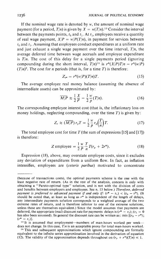
If the nominal wage rate is denoted by w, the amount of nominal wage payment (for a period, T/n) is given by X = avi(T/n).13 Consider the interval between the payments points, to and t1. At t1, employees receive a quantity of real wage payment, X/P = w/P(T/n), in payment for services between to and t1. Assuming that employees conduct expenditures at a uniform rate and just exhaust a single wage payment over the time interval, Tln, the average deferred time between wage accruals and employee expenditure is Tin. The cost of this delay for a single payments period (ignoring compounding during the short interval, T/n)'4 is r*(X/P)T/n = r*(w/P) (T/n)2. The cost for n periods (that is, for a time T) is therefore:
Zr* = r*(w/P)(T/n)T. (15)
The average employee real money balance (assuming the absence of intermediate assets) can be approximated by:
1/ IX 1w (l6) M/P y2 P 2 2-(T/n) (16)
The corresponding employee interest cost (that is, the inflationary loss on money holdings, neglecting compounding, over the time T) is given by:
Zr (M/P) rpT hr T( (17)
The total employee cost for time T (the sum of expressions [15] and [17]) is therefore:
Z employee = I
-T(r, + 2r*). (18)
Expression (18), above, may overstate employee costs, since it excludes any deviation of expenditures from a uniform flow. In fact, as inflation intensifies, employees are (ceteris paribus) motivated to concentrate
(because of transactions costs), the optimal payments scheme is the one with the least negative rate of return. (As in the rest of the analysis, concern is only with obtaining a "Pareto-optimal type" solution, and is not with the division of costs and benefits between employers and employees. See n. 15 below.) Therefore, deferred payment is preferred to advanced payment if and only if: (r* -- rL) < (rB - r*). (It should be noted that, at least as long as r* is independent of the length of delays, any intermediate payments solution corresponds to a weighted average of the two extreme rates of return, and is therefore inferior to one of the extreme solutions, unless these are themselves equivalent.) Since the model assumes that payments are deferred, the appropriate (real) discount rate for payments delays is (r* - rL); (rL = 0 has also been assumed). In general the discount rate can be written as: min [(rB -r*); (r* - rL)].
13 It is assumed that employment-numbers of man-hours worked per week- does not change. In this case, Tln is an acceptable proxy for total man-hours worked.
14 This and subsequent approximations which ignore compounding are formally equivalent to the infinite series approximation involved in the derivation of equation (12). The validity of the approximation depends throughout on (rQ + r*)(Tln) << 1.

INFLATION AND DEMAND FOR MONEY 1237
expenditures closer to payment times in order to reduce money holdings and incur smaller losses from inflation. However, a preliminary model of this behavior suggests that the general relationship between average money holdings and the rate of inflation is not materially altered by a considera- tion of this motive. This conclusion is further supported by the observation that, while employees desire to concentrate expenditures shortly after wage payments, employers have a symmetric desire to concentrate expenditures just before payments. The balancing of these forces could generate a "weekly seasonal" of rate of price change that would dis- courage the concentration of expenditures either just after or just before wage payments, and tend to restore the system to a uniform pattern of expenditure. In any case, the assumption of uniform patterns is retained in the body of this paper.
With the assumption of uniform expenditure streams, total real costs over time T (the sum of employer and employee costs) are given (from equations [13] and [18]) by:
Ztotal T{[ (2 + - )rp + r*] + T} (19)
The optimal-payments period is that value of Tln which minimizes this total cost expression.15 Accordingly, we have: aZ/a(T/n) = T[! (YIP + w/p)rp + w/p r* -(a/p)/(T/n)2] = 0. Therefore:
7' = Jl(alP)/[2 ( + )rrp + ? ]r* (20)
If we assume w1P Y/P,16 we can write:17
- V1(a/P)/[Y/P(r, + r*)]. (21) n
The second-order minimum condition is satisfied for this solution.
15 This cost minimization guarantees a Pareto-optimal situation with respect to employers and employees. For example, if employees were willing to pay some amount (in the form, say, of a reduced explicit wage) for a reduction in the payments period, and employers were willing to accept some lesser amount as compensation for this reduction, it is assumed that the reduction of the payments period takes place. The division of costs and benefits between employers and employees is not discussed explicitly-largely because it does not seem necessary for the desired results.
16 In effect, Y corresponds to the total money flow into a business and w to the total money flow out of a business. (That is, w comprises rentals, payments to other businesses, net earnings, et cetera, as well as payments to labor-although the real discount rate, r*, may depend on the particular form of payment.) Therefore, syste- matic deviations between YIP and w1P can occur only through intermediate inflation- ary losses. This loss relates to the cost of inflation (equations [19] and [22]) and increases with (r, + r*)l/2. However, as long as r, is less than astronomical, this cost remains small relative to YIP, so that the approximation YIP - wlp should be sus- tainable.
17 The payments-period relationship, equation (21), can be readily extended to the case where satisfactory intermediate assets exist (see previous discussion). In one

1238 JOURNAL OF POLITICAL ECONOMY
TABLE 1 RELATIONSHIP BETWEEN PAYMENTS PERIOD
AND RATE OF INFLATION*
rp (% per Month) Tln (Months)
0 . . . . . . . . . . .5 (2 per month) 1 . . . . . . . . . . .35 (3 per month) 3 . . . . . . . . . . .25 (1 per week)
15 . . .125 (2 per week) 50 . . . . . . . . . . .07 (every 2 days)
200 . 035 (daily)
* As implied by equation (21).
While it is possible to discuss only orders of magnitude, it is interesting to explore the relationship between the payments period and the rate of inflation implied by equation (21). For example, taking parameter values of Y = $400 per month, a = $1.00 (only the ratio a! Y is of importance in equation [21]), and r* = .01 per month, the relationship as shown in table 1 holds.
While the exact relationship depends on the arbitrary specification of parameters, the overall magnitudes accord with observations from some extreme inflationary experiences.18 An interesting implication of the above
plausible situation, employers have available (at a transfer cost which, in the overall cost calculation, is low enough to make the asset worthwhile) an alternative asset with (riskless) real rate of return, rL, and employees have available no satisfactory alternative asset. In this case the real rate of return on employer money holdings is changed from - r, to rL, and the remainder of the model is unchanged. Therefore, (r, + r*) in equation (21) is replaced by (r* -r - -rL) to yield the new optimal payments period. If employees have access to a similar satisfactory asset, (r, + r*) in equation (21) is replaced by (r* -rL). In this case, the determination of a finite payments period requires the real discount rate of employees (r*) to exceed the underlying (riskless) real rate of return (rL).
It should be noted that the decision to employ an alternative asset involves a weighing of the rate of return against the cost of transactions relative to the volume of transactions. Therefore, considering their larger scale of transactions, employers are more likely than employees to find a particular asset (with given rate of return and transactions-cost characteristics) satisfactory, so that the first case (with rate: r* + Ir, - IrL) may be the most realistic-at least for developed countries like the United States. For countries that are experiencing extreme inflations (such as those studied in Part II of this paper) the complete exclusion of intermediate assets seems most realistic, and equation (21) applies directly.
18 For example, in 1923, the final year of the German hyperinflation, "it became the custom to make an advance of wages on Tuesday the balance being paid on Friday. Later, some firms used to pay wages three times a week, or even daily" (Bresciani- Turroni 1937, p. 303). The range of ("effective") rates of inflation in this period was 20-300 percent per month (see table A2). Similarly, during the Austrian hyperinfla- tion, "the salaries of the state officials, which used to be issued at the end of the month, were paid to them during 1922 in instalments three times per month" (Walre de Bordes 1924, p. 163). During 1922 the (effective) rate of inflation reached a peak value of about 45 percent per month (see table Al).

INFLATION AND DEMAND FOR MONEY I239
relationship is the comparatively minor adjustment in the payments period necessitated by astronomical rates of inflation. Even at the extraor- dinary rate of 200 percent per month, payments are made only once per day. While this high frequency of payment involves additional bother (amounting to one-half of the inflationary cost of equation [22]), it cannot be viewed as an intolerable burden. Therefore, it is not surprising that (depending on the types of substitute payments media available) the benefits of money as a transactions medium could outweigh the inflationary cost, and induce persons to retain money at rates of inflation (as high, say as 100-200 percent per month) at which casual analysis might suggest a total flight from money.19
Substituting the result of equation (21) into equation (19), using YIP w/P, we obtain an expression for total (minimized) inflationary cost over time T: 20
Ztotal 2TVa/P(Y/P)(r, + r*). (22)
C. The Demand for Money and Money Substitutes
Using the approximation for employer money balances in equation (14) and the analogous expression for employees in equation (16), aggregate real balances can be expressed as:
M/P= M/Pempioyers + M/Pemployees
l YT lwT -2P + 77 (23) 2 P n 2 2P n-(3
Taking Y/P h?/P and substituting for T/n from equation (21), we obtain (omitting the bar over M/P):
M/P /(a/P)(Y/P) (24) M (r +~ r*)
(4
If transfer costs (a/P) are totally of an income-forgone nature (a/P Y/P), then:
/P AY/P _Vrp + r*
where A = V/(a/P)/( Y/P) is taken as a positive constant. In the analysis of Sections A and B, money was retained as the sole
payments medium. Within this framework, there emerged an inverse
19 In this regard see Keynes 1924, pp. 48-50. 20 The cost due to the inflation rate r, requires a subtraction of the r* portion from
equation (22):
Zrp = 2T J p (Vrp + r*- vr*).

1240 JOURNAL OF POLITICAL ECONOMY
relation between real cash balances and the inflation rate (equations [24] and [25]). The mechanism by which cash holdings were reduced in response to a higher rate of inflation involved the reduction of the time period between transactions (that is, an increase in velocity). An additional mechanism by which cash holdings could be reduced involves the sub- stitution of some alternative asset (foreign exchange, private tokens, payments in kind, and so on) as a transactions medium. By reducing the set of transactions to which money is applied, average cash holdings can be reduced, even if transaction periods (velocity) remain constant.
Letting 5P(r,) denote the fraction of transactions (as a function of the inflation rate) which are conducted via some substitute medium, and assuming that the analysis of Sections A and B applies to the 100(1 -) percent of transactions for which money is retained, we have from equation (25):
M/~ [1 -
P(r,)] -A YIP (6 /Vrp + r* (26)
The elasticity of real cash balances with respect to the inflation rate is (from equation [26]):
cr(M/P) rp ( rp -
rp V(rp) arP MIP 2 rp + r*) I - (rp)
Therefore, if the percentage of monetized transactions does not respond to rp[(D'(rp) = 0, P(rp) < 1], the elasticity is given by the first term on the right-hand side of equation (27). In this form (with r* > 0), the (absolute) elasticity rises from zero at rp =0 and asymptotically approaches I as rp becomes large relative to r*. On the other hand, if the percentage of substitutes responds positively to the rate of inflation ['F'(rp) > 0], the right-hand term in equation (27) adds (possibly in an increasing fashion) to the (absolute) elasticity. Stated another way, if the percentage of money substitutes is constrained to be unresponsive to the inflation rate (and, therefore, if increases in velocity are the only method for reducing real money holdings),21 there would exist a limiting elasticity of real cash balances to the inflation rate. When the possibility of varying the per- centage of monetized transactions is recognized, there exists the potential for an indefinitely increasing elasticity.
Once the percentage of monetized transactions (1 - $) is regarded as a behaviorally determined magnitude, it is necessary to construct an explicit cost-benefit framework for determining the mode which payments take. If money is used for a volume of transactions corresponding to
21 It should be recalled that variations in the shape of expenditure streams have been ruled out. However, this type of variation does not appear to be a potential source of an increasing inflation-rate elasticity.

INFLATION AND DEMAND FOR MONEY 124I
YIP, the inflationary cost per unit of time is (from equation [22], using A = -V[a1P]1[Y1P]):
T = 2A(Y/P)( Mr+r* - ) (28)
If a stable-valued asset is substituted as the transactions medium, the above cost could be avoided. Therefore, the decision to employ money or the substitute involves a comparison of the inflationary cost (equation [28]) with the benefits of money as a transactions medium (in terms of physical convenience, general acceptability, et cetera). The size of this benefit cannot be readily quantified, since it depends on the type of transaction and the individuals involved. For example, the benefit is likely to increase as one moves along the following list: (1) transactions within a family, (2) regular dealings with a local merchant, (3) dealings in new locations, (4) payments by mail, (5) dealings in securities markets. In any case, it seems feasible to group transactions into homogeneous classes, within which the benefit per amount of transaction is constant. That is, for the ith group of transactions, the benefit (per unit of time) of employing money is:
Bi (T/P)(l - P'i)( Y/P)L, (29)
where, (1 - (Di) is the fraction of the ith group's transactions which use money; and (T/P)i is a constant for the ith group. The net benefit from employing money (over the stable-valued substitute) is (from equations [29] and [28]):
Ri = (1 - (FP)(YIP)i[(F/P)i -2A(VriTV* - Vr*)]. (30)
If the expression in brackets is positive, it will be advantageous to employ money for all transactions of the ith group ((Di = 0), while if the bracket expression is negative, the ith group should abandon money entirely (@i = 1). Therefore, the criterion for employing substitutes for the entire volume of transactions corresponding to (YIP)i is:
(Tf/P), < 2A(Vr, + r* - /*). (31)
Given the group criterion of equation (31), and assuming that A, rp, and r* do not vary among different groups, the overall percentage of substitute transactions as a function of rp is determined by the joint distribution of (T/P)i and (Y/P)i. In the absence of direct empirical evidence on this distribution, an aggregate relation for subsequent empirical analysis is derived from the following (semiheroic) assumptions: (1) (T/P)i and (Y/P)i are independently distributed; (2) the distribution of (T/P)i satisfies

1242 JOURNAL OF POLITICAL ECONOMY
certain boundary conditions,22 and can be adequately described by a (second-order) gamma distribution (Hogg and Craig 1965, pp. 91-93):
Pr[(T/P)i < x] = 1 -(1 + Ax)e-x (x > 0) (32)
Pr[(T/P)i < x] = 0 (x < 0)
where, Pr may be interpreted as a cumulative probability. With the above assumptions, the overall percentage of substitute transactions is:
q) = Pr[(f/P)i < 2A(Vr- + -r* - V)]. (33)
Letting k = 2AA, we obtain from equation (32):23
qP = 1 - [1 + k(Vrp + r -Alr Ae ITP +r*- /;) (rP > 0), (34)
(D = ? (rP < 0).
Using equation (26) we obtain the demand-for-money function:
/ = A Y/P * (1 --/j; M/P Vr I + r* [I + k(Vlrp + r* - )]ek(rp+r-Vr) (r 0),
(35)
M/P = Ar (-Pr* < rp < 0)24 V/rP + r*
In equation (32), the "expected value" of (W7P)i is (T/P) = 2/A. Therefore, in equations (34) and (35), k = 4A/Q(/P) is a parameter which is inversely related to the average cost of employing money substitutes. The higher this average cost, the smaller the percentage of money sub- stitutes (equation [34]), and the larger the demand for the conventional money supply (equation [35]) for a given value of rp.25
The inflation-rate elasticity from equation [35] for large values of rp is:
MrP M/P ( k 2r ~~(M/P) r - I+ krP) (rp> ?r*). (36)
22 (l) f(X) = 0 for x < 0 (see n. 24), (2)f(x) is skewed to the left for positive values of x, (3) f(x) is approximately exponentially declining for large values of x. While the (second-order) gamma distribution is only one possible distribution that satisfies these properties, some others which might be considered (such as, log normal) have cumulative distributions which cannot be integrated in closed form.
23 By adopting the boundary condition (D(r, = 0) = 0, we ignore the possible use of money substitutes when r, < 0. Actually, a positive rate of return on money holdings (r, < 0) may be required in order to induce certain nonmonetary sectors of the economy (especially prevalent in underdeveloped countries) to employ the conventional money supply.
24 The situation with r, < r* is unstable because the real rate of return on money holdings (-r,) exceeds the marginal impatience rate, r*. The stability properties of the system will be discussed in a later paper.
25 The percentage of money-substitute transactions, as a function of the rate of inflation, is illustrated in the table below. Parameter values of k = 1.25 (months 1/2)
(the empirical estimate for Germany) and r* = .01 per month have been used.

INFLATION AND DEMAND FOR MONEY 1243
Therefore, the (absolute) elasticity increases with r, beyond I, with the rate of increase depending on k. While the precise form of equation (36) hinges on the assumed distributions of (T/P)i and (Y/P)i, the general behavior depends only on an increasing tendency to adopt substitutes as rp rises, and has already been described in equation (27).
In equation (35), which assumes that transactions costs, aIP, rise proportionately with Y/P, the elasticity of real cash balances with respect to real income is constant at + 1.0. If transactions costs rise less than in proportion to YIP, the elasticity is reduced and "economies-of-scale" in cash balances are realized. If transactions costs rise more than in pro- portion to YIP, the elasticity exceeds + 1.0 and money is a "luxury."26
D. The "Effective" Rate of Inflation
Equation (35) indicates the quantity of real money holdings, MIP, corre- sponding to a steady rate of inflation, rp. If the inflation rate varies over time, equation (35) does not carry over directly, since the underlying optimization assumes that the single rate rp persists forever (or, at least, that all economic actors behave as though they believe in a constant rate). If the rate of inflation is not constant, we can define an effective rate of inflation, rt, as that "perpetual" rate which corresponds to the current (demand for) real balances in the form of equation (35). That is:
(M/P)t - ? r+ [I + k(V\7rt + r*- Vr*)] e k(Vf +r - -r) (7 ? 0)
(37)
(MIp)D AY/P (-r* < ,e < 0), V/7r + r*
where, we maintain the assumption that YIP and r* are fixed.
rp (% per month) 'D(%7)
0 . . . . . . . . . . ... 0 1 . 0.2 3 ...... . . . . . . 0.8
15 ...... . . . . . . 5.5 50 . . . . . . . . . . . . 18.0
200 ...... . . . . . . 49.2
Therefore, if the form of the distribution and the estimated k value are accepted, money substitutes become important only under the most extreme inflationary conditions.
26 This result assumes that changes in YIP do not, ceteris paribus, produce changes in the percentage of transactions which are monetized. One might argue that an increase in overall real income (development) is associated with shifts to types of

1244 JOURNAL OF POLITICAL ECONOMY
If iT, denotes the actual rate of inflation, (l/P)(dP)/(dt), at time t, the steady-state model suggests the boundary condition: rt = rp constant, for t = -o, + ?? > 7T = rp, where, 7Tt at future times may be inter- preted here as a fully expected (7Tt = rp with probability 1) rate of inflation.
In the general case we require behavioral assumptions that go beyond the steady-state model.
The statement that (M/P)l is related to ,e in the form of equation (37) amounts to the statement that 7te determines such fundamental decision variables as the payments period and the percentage of money substitutes in a manner which leads to the prescribed form for money demand. Accordingly, T/n (for those transactions which retain the conventional money supply) is given from equation (21) as:
(T/n)t-I Y/P(7rt + r*) (38)
and the percentage of money substitutes by :27
(Pt I1 - [1 + k(Vr~t+ ?r* - Vl.*)]e k(7t+r r) (Tt ? 0),
(39) ot 0 (77t < 0).
Presumably, values of (T/n)t and 4t (with implied values of 7t) are chosen over time so as to minimize some conception of inflationary costs. In attempting to quantify these costs below, we neglect the influence of money substitutes (take k 0) in order to keep the algebra manageable.28
Assume that the actual rate of price change, ITt, prevails over some time interval, T. The cost associated with maintaining an effective rate, t7e, over this interval is:
Z = T[(M/P)(-,t + r*) + = -T [-4(2t ? r*) + T4]. (40)
transactions in which the benefits of money as a payments medium are high (T/P increases as YIP increases-though this is likely to contradict the previous simplifying assumption that [F/P]i and [Y/P]i are independently distributed). In this case the income elasticity is raised, and money is more likely to emerge as a luxury.
27 It is assumed that the same 7, value is appropriate for Tin, D, and any other decision variables that are relevant for (M/P)D.
28 Essentially, we concentrate on the payments period as a decision variable, and therefore restrict attention to individuals who retain the conventional money supply. As far as relative shifts in and out of substitutes (changes in 0) differ from relative shifts in the payments period, some error will be introduced in the generation of 7e*
The error is likely to be small for small values of qD (see n. 24), and may become important as 1D becomes large. However, the direction of error is not immediately clear, and further analysis would be required to ascertain it.

INFLATION AND DEMAND FOR MONEY 1245
Substituting for Tin from equation (38) (with A [a/P]/[YIP]) we obtain after simplifying:
Z = TAYP (t + r* + 7Te + r*). (41)
If rTe is set equal to the actual rate, ATts the cost is (assuming 7Tt + r* > 0):
Z = 2T(A YIP) Vart + r*. (42)
Therefore, the cost of maintaining an effective rate different from the actual rate (over time T) is (after simplifying):
Z Z = T.A P (\aTt + r* - T + r*)2. (43) A1T + r* (V
Clearly, the minimum cost, Z - Z = 0, obtains at ni = Xt.
Presumably, if rt were perceived instantaneously, and 7Te (that is, Tin and other implied decision variables) could be adjusted costlessly with a zero time lag, we would always have e = vt. Assuming that the lag in perception of Tt can be neglected, the essential characteristic for the existence of 7t # vt is a nonzero cost associated with changes in ve (that is, with changes in Tln, et cetera). Let a denote the real (fixed) cost attached to making changes in Tre (the cost is assumed to be invariant with the amount of the change). In general, if 7Te is varied more frequently, the a cost rises, but the average cost of being out of equilibrium (setting VV e + r* =A V/7r + r* is equation [43]) declines. The complete descrip- tion of the tradeoff requires a specification of the mechanism by which v
is generated. The model adopted here involves the application of an (S, s) policy to a
stochastic inventory model of the type utilized by Miller and Orr (1966) in a different context. Assume that at time zero an economic unit has just adjusted its effective rate to equal the current actual rate (0-O =
Future actual rates are assumed to be observed as averages over discrete time periods: 7fT V2T7. .* with a fixed observation interval, ar. The variable, aVt + r*, is assumed to follow a symmetric random walk with fixed step size c, beginning at V7v0 + r* at time zero. That is, VBUT + r* = y'ijT+ r* ? e with probability 2, and Vi/r + r* - E with probability 1; VI2v + r* = /Vir + r* + E with I probability each, and so on. The economic unit selects ceiling and floor values of \/r + r*, V/7ro + r* + hu and \/TO + r* - hL, at which adjustments in 7re occur (that is, the unit sets Vnre + r* =
N/vo + r* + hu if the ceiling is reached, and V1Te + r* = V/v0 + r* -hL
if the floor is reached).29 Because the cost of being out of equilibrium is
29 The realism of this process can be questioned on two (interrelated) levels: (I) Do individuals behave this way? (2) Does the actual course of rates of price change approximate a random walk? Since 1t is endogenous at the aggregate level, the second

1246 JOURNAL OF POLITICAL ECONOMY
symmetric about Pro, an optimal solution involves hU = hL = h.30 The higher the selected value of h, the smaller the adjustment (U.) cost, but the larger the average out-of-equilibrium cost. The tradeoff is formalized below.
Let x = (V/7rt ? r* - e + r*)/E denote the random variable (with zero origin and unit step size) which is subject to the random walk. The density of x is determined by the difference equation:
f(x,t) = f(x - 1, t - 1) + I
f(x + 1, t - 1); x = 0; - h < x < h-
(44)
Confining attention to the steady-state distribution defined by:
f(x) = f(x- 1) + f(x + #);x 0 0;- h < x < - (45)
with boundary conditions:
f(h/E) = f(-Ih/E) = 0,
f(0) = I [f( - _) + f(-1)] +
I - h + 1 + f(+ 1)] (46)
h/c
Z f(x)=l, x= -hIE
the equation can be solved in the form f(x) = A1 + B1x (x > 0),f(x) =
A2 + B2x (x < 0).
question involves, in particular, the behavior of the rate of change of the money supply. Because the random-walk process is nonstationary, it is unlikely to provide a realistic long-run description of the rate of price change or of the rate of change of the money supply. Nevertheless, the process may provide a useful basis for short-run analysis of individual adjustment behavior. In any case the important assumptions seem to be: (1) a fixed perception interval, r, (2) the symmetric nature of the walk, and (3) serial independence. The second assumption reflects a (long-run) neutral stance toward acceleration or deceleration of prices, and appears to be reasonable. The third assumption (which rules out extrapolations of the recent mt trend) is more questionable. Serial dependence would affect the form, though not the general nature, of the results. The first assumption is critical for the model, and reflects a segment of behavior that has not been considered at all. Essentially, the random-walk proc- ess regards any observed value of ITt as the best estimate of future 7T values. Accord- ingly, no distinction is made between expected and actual rates of inflation, and the explanation for rt4 # 7t derives solely from costs of adjustment of we. As the percep- tion interval (r) tends to zero, the model implies that each instantaneous value of (I/p)(dp)/(dt) is, by itself, the best estimate of future -t's. Maintaining a finite value of r substitutes an average value of (l/p)(dp)/(dt) for an instantaneous value, but does not change the fundamental problem. A complete model would consider both expectational and adjustment factors in the formation of the effective rate (ITe), and would remove the ad hoc perception interval that was necessitated by the lack of an expectations mechanism.
30 This is a slight approximation, based on the discussion in n. 34 below.
INFLATION AND DEMAND FOR MONEY 1247
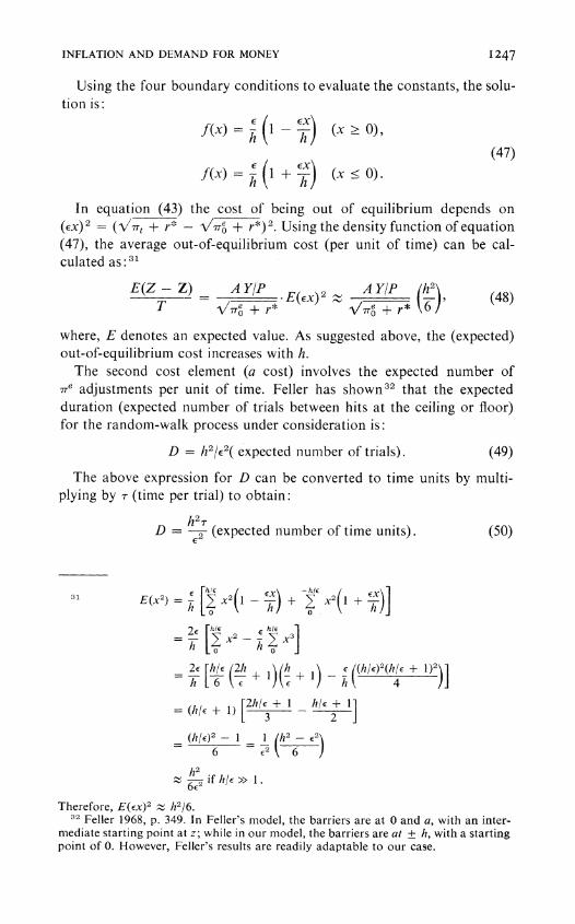
Using the four boundary conditions to evaluate the constants, the solu- tion is:
f(X) = EX( -h (X > 0),
(47) f(x) = h (1 + e) (x < 0).
In equation (43) the cost of being out of equilibrium depends on (EX)2 = (vVt + r* - V0 + r*)2. Using the density function of equation (47), the average out-of-equilibrium cost (per unit of time) can be cal- culated as:31
= - A E(-X)2 A Y * (h)' (48)
where, E denotes an expected value. As suggested above, the (expected) out-of-equilibrium cost increases with h.
The second cost element (a cost) involves the expected number of 7re adjustments per unit of time. Feller has shown32 that the expected duration (expected number of trials between hits at the ceiling or floor) for the random-walk process under consideration is:
D = h2/E2( expected number of trials). (49)
The above expression for D can be converted to time units by multi- plying by r (time per trial) to obtain:
h27 D =
E2 (expected number of time units). (50)
31 E(x2) = 6 [2 x2(1 - h) + j x 2(1 + )
= _2 - X3]
= h [E (6 + 1 + 1-h ((h/E) (h!E + 1))]
(h/ + 1) [2h/E? 1 _ h/E + 1]
(h/E)2- 1 I _h2-E2
6 E2 6
h 2
-62 if h/lE> 1.
Therefore, E(Ex)2 h2/6. 32 Feller 1968, p. 349. In Feller's model, the barriers are at 0 and a, with an inter-
mediate starting point at z; while in our model, the barriers are at + h, with a starting point of 0. However, Feller's results are readily adaptable to our case.

1248 JOURNAL OF POLITICAL ECONOMY
The above expression measures the expected amount of time between contacts with the upper or lower barrier (that is, between adjustments of 1e). The expected number of contacts (adjustments) per unit of time can be approximated by 1/D (see Miller and Orr 1966, p. 421).
Letting m denote the number of contacts in time T, we have:
E(m/T) l/DD -=2 (51)
As suggested above, the higher h, the lower the (expected) number of adjustments per time, and the lower the associated (expected) a cost.
The variance of the Bernoulli process involved in the symmetric random walk can be derived (as a function of time) as Cut = (E2/r) t, where t denotes the total elapsed time since the start at time zero.33 At t = 1 (month) the variance is:
a72 =-6 = monthly variance of V-rrt + r* (52)
Therefore, the expected adjustment cost per unit of time may be written (from equation [51]) as:
a2 E(Za) = a. E(m/T) = a * (53)
The total expected cost per unit of time (as a function of h) is (from equations [48] and [53]):34
E(cost/time) E(Z - Z) + cc E(m/T) T
_ A YIPor = V +e h2 +
a.2. (54) 6 0/r + r*
The value of h2 that minimize this expected cost is given from a(Cost)/ah2 = 0 as:
h2 A Or6 X/p a(lTO + r*)4 (55)
On an individual level, ire is shifted or kept constant according to whether a newly observed value of art is sufficient to reach a ceiling or floor (with the ceiling and floor positions determined from equation [55]). The
3 See Miller and Orr, p. 419. This unconstrained variance is, of course, derived independently of the barrier positions at +? , and, therefore, does not correspond to E(ex)2, which was calculated above.
34 This analysis neglects the fact that subsequent starting points do not correspond to the initial point (\/ e + r*). In fact, the starting points conform to a modified symmetric random walk with stochastic time interval and varying step size. Since the process is symmetric, neglecting it may be a satisfactory first approximation.

INFLATION AND DEMAND FOR MONEY I249
aggregate 7Te behavior depends on the proportion of units that attain ceilings or floors in a particular time interval. An approximation to the aggregate response is described below.
Assume that a particular value of Ex = VNrt + r* - V0r + r* pre- vails at some time. The likely conclusion of the random walk which origi- nates at x (that is, the relative probabilities of hitting the ceiling or floor first) depends on the position of x relative to h and -h. It can be shown that (see Feller 1968, p. 345):
Pr(+ h) = h + Ex 2h
(56)
Pr(-h) = 2h -E
where Pr(+h) is the probability of terminating at +h when the process originates at x, and analogously for Pr(-h).
The expected duration of the walk which originates at x is (Feller, p. 349):
D = (h - Ex)(h + EX) (57) ar2
Therefore, the expected number of adjustments per time is:
U2
E(m/T) x= (h - Ex)(h + EX) (58)
The expected number of ceiling hits per time can be approximated by:
M + o~~~~~r2 (9 E(jy) ~ Pr(+h).E(m/T) 2h(h + EX))
Similarly, the expected number of floor hits is:
E( LI' Pr(- h) E(inlT) - (60) \T /2h(h - Ex)'
Each ceiling hit produces an increase in (an individual's) \/7re + r* by h, and each floor hit a reduction by h. The net (expected) change in ve+r* is given by:
d (V7T
? r*) . h4Emj - E 'nT)] dt ( )~h[tT ) (T )
(61) or2 C 1 2EX or2Ex
2 (hex h + ex h2 _ (EX)2 h2
(if h >> EX).35
3 That is, the original (in effect, average aggregate) deviation, Vot + r* -
Vote + r*, is assumed to be small relative to that deviation (h) which produces a shift in w.

1250 JOURNAL OF POLITICAL ECONOMY
Substituting Ex = (V I7V7r - I )e+ r*), and h2 = h2 from equation (55):
d + (YP'(e + r*) - P(V1t ? r* - +r. dt 6 (62)
Equation (62) describes the expected change over time in (an individ- ual's) ~e ? r* as a function of the current gap (Vot + r*- aV ? r*). With the additional (difficult to evaluate) assumption that the average aggregate value of /7rt + r* - /7T + r* yields a satisfactory approxi- mation to average behavior in the form of equation (62), the relationship can be used to explain the trend over time in the average aggregate value of ir, which is assumed to be relevant for aggregate money demand in the form of equation (37).
The first term on the right side of equation (62), [(A Y/P)/6a]1/2, may perhaps be satisfactorily regarded as a constant. However, a, the square root of the monthly variance of I , generally depends on the intensity of inflation. Provisionally, this dependence is approximated in the following manner.
Let [t = (l/M)(dM/dt) denote the proportionate rate of change of the money stock. The corresponding amount of inflationary-financed (govern- ment) expenditure is: GM = At M/P. Assuming MIP M/PD and
At , we have (from equation [37] with k 0):
dt dT( M/P) 2 (1 + + r*) dt* (63)
Therefore:
dl- 2 (1 r* dGM WTi ui/~ A+ 2r~j!dt (64)
If government expenditure is financed by a combination of money creation and tax revenues (G = GM + GT) we have:
dG =dGM dGT (5 dt dt +F dt (65)
If the primary function of inflationary finance is to offset (unexpected?) variations in tax revenue (that is, dG/dt 0), we have:
dGM _ dGT (66) dt -dt(6
Letting 0 denote the proportional rate of change of nominal tax revenues, we have:
dG GT[O - f] (67)

INFLATION AND DEMAND FOR MONEY 1251
Therefore, the magnitude of fluctuation in tax revenues depends on the average magnitude of IO - r. Provisionally, we assume that this average size is proportional to _rre. In this case:
dGT g. 7,e (g = constant). (68)
Therefore, from equations (66) and (64):
|d | 2gl/e (1 - r*) (69) dt ~M/P u+2i
Using [ e, M/P t M/PD, and substituting from equation (37):
+ r*, ~AY/P 1 _ (I - e + 2r(70)
where (P is given by equation (39). If Id/(dt) V/Ir + r*I can be approximated by Id/(dt) / + r*j, and if
a (the monthly standard deviation of A+r*) is proportional to Id/(dt) x V/r + r*I, we have (from equation [62]) a mechanism for generating
effective rates of inflation:
dtV/e? r* b*(e + r*)l/4 (1 _ (l E + 2r* _
x ( r*~ V /7,e + r*), (71)
where b = constant > 0. If e>> r*:
d e_____ e) Vt /7Te b(Te)3I4
- _ (,\/7r- - (72) dt (1 (P)D -V~)
The mechanism in equations (71) and (72) may be compared with the original adaptive-expectations model (Cagan, p. 37):
dt (7,e) = Y(,r- _ e), (y > 0). (73)
The new mechanism differs in two respects. First, as a reflection of the underlying inflationary costs, the mechanism (equations [71] and [72]) emerges in square root, rather than linear, form. Second, the coefficient of adjustment is not constant, but increases with the rate of inflation (with (7Te)3/4[1/(l - (I)] in equation [72]). Cagan's empirical results suggested that a rising adjustment coefficient might be a more appropriate mechanism (Cagan, pp. 58-64). The current model provides a theoretically derived mechanism of this type, which is used for an empirical study in the second part of this paper.

I252 JOURNAL OF POLITICAL ECONOMY
II. Empirical Results on Demand for Money during Hyperinflations
The theoretical model of demand for money has been applied to data on four post-World War I hyperinflations (Austria, Germany, Hungary, Poland) previously studied by Cagan (1956)36 and Allais (1966). The data for each case differ somewhat from that employed by Cagan, and are described briefly in the Appendix tables. The demand-for-money function is derived from the theoretical model (equations [37] and [39]):
log(M/PD)t = ac- + U-2.l0g(9re + r*)t + log(1 - (4t) + Ut, (74)
where:
(1 - t) = [I + k(Ve+ r* - Vr*)tjek(vze+r - ) (t ? 0); (75)
(1 -at)= 1, (-~~~~~~~r* < 7Te < 0);
and ut is thought of as an independently, normally distributed disturbance term. In the theoretical model, a, = log (A Y/P) (though this coefficient is likely to be affected by aggregation) and a2 = -0.5. We have assumed, additionally, for the current empirical study that Y/P z constant; r* constant ~0; (M/PD)t (M/P)t.
The accuracy of Y/P % constant for the relatively short hyperinflation- ary experiences under consideration has been discussed in Cagan (pp. 97-114). The type of information that Cagan considers can be used to construct rough employment indices for the four cases. These indices are contained in the Appendix tables. Considering the coverage and accuracy of the basic data, the indices seem fairly reliable (as a general indicator) for Austria and Germany, less reliable for Poland, and mostly unreliable for Hungary. The overall indication is that variations in real income were small relative to changes in the inflation rate, so that taking Y/P con- stant may be satisfactory (though this conclusion is especially questionable for Hungary and uncertain for Poland). Because of the crude nature of the employment data, the addition of real income to the regression equations has not been attempted.
In general, the real rate of discount (r*) should be somewhat above the (riskless) real rate of return in an economy. Average real rates of return during the hyperinflations were apparently small and possibly negative. Accordingly, we expect values of r* near zero, and, in any case, negligible in comparison with the inflation-rate variable (ire). Therefore, we have set r* = 0 and have not attempted to estimate r* from the data.
36 Three cases from Cagan's original seven have been excluded: post-World War I Russia and World War II Greece and Hungary. The Russian case was excluded because the assumption of constant real income appeared unreasonable and adequate income data was unavailable. The money-supply data for Greece was unreliable (Cagan, p. 106), and the variation in real income during the war was apparently substantial (International Labor Review, December 1945, p. 650). The available data for Hungary covers too brief a period to provide a useful test of the model.

INFLATION AND DEMAND FOR MONEY 1253
The possible error involved with taking M/PD = M/P is not explicitly considered in this paper.
The effective rate of inflation (7Te) in equations (74) and (75) is assumed to be generated by the mechanism of equation (72):
d i W-e = b(re)314 I1 (1 -;; -V/r), (76) d (I - 4)gii
where, 'D is given in equation (75). Since the model is applied to discrete (monthly) data, a discrete approximation has been used :37
7/rt a t + (
p- t) e/7-
t = 1 - eb(at) (3 i ) (77)
where, Tt is the average rate of price change over the interval (t - 1, t), Xe = (7Te + 7TD and t = )
The coefficients to be estimated for each case are a1, a2, k, and b. The method of estimation is a nonlinear iterative routine for minimizing the sum of squared residuals in each regression. This procedure corresponds to maximum likelihood estimation if the error disturbances (Ut) are independently and normally distributed.38 Since the primary objective is to test the theory, we list the a priori conjectures on each coefficient:
1. a 1 = log (A Y/P): Without information on real income levels, this coefficient depends on arbitrary index levels, and cannot be tested.
2. a2 = -0.5: This point value is the strongest a priori information to be tested.
3. k: This parameter determines the percentage of money substitutes (4)) as a function of 7Te (equation [75]). The higher k, the larger the per- centage of substitutes and the smaller the demand for money at a given value of ire: k = 4A/(F/P) = 4Va/ Y/Q(T/P) (see Section IC), where a! Y is the ratio of transactions cost to transactions volume and T/P is the average cost of employing money substitutes (per amount of transaction). To obtain some notion of the order of magnitude of k, we assume (taking time units of months), 0.5/400 < alY < 2.0/400, .10 <_ T/P < .20. Correspondingly, the limiting values of k- are 0.7 < k < 2.8 (months1/2).
Negative values of -7T were set equal to zero in order to obtain Virt in equation (77). In fact, few negative values occurred so that no major adjustment was required. Nevertheless, the necessity for this adjustment reflects an incompleteness in the generation mechanism for ,e, which may stem from the lack of an expectations mechanism (see n. 29).
38 See Cagan, pp. 93-94. One problem with the estimation is that Pt influences both sides of the equation. This problem is not serious when Pt << 1, but may become important for the most extreme observations. Unfortunately, obtaining a reduced form equation does not seem possible.

I254 JOURNAL OF POLITICAL ECONOMY
Obviously, this limit is both wide and arbitrary, but k > 0 is a funda- mental implication of the theory: k = 0 (an infinite cost for money sub- stitutes) corresponds to a constant inflation-rate elasticity, while k > 0 corresponds to an increasing (absolute) elasticity. The model is supported if k = 0 can be rejected in favor of k > 0.
The k parameter may also be viewed in terms of its variation among different cases. The theory suggests (for given values of a! Y) that k is larger the smaller the value of T/P. Therefore, higher k values correspond to situations where money substitutes are more readily available (that is, less costly). However, there is little a priori basis for determining relative T/P values among the cases studied, so that equality among the k values forms the basic null hypothesis.
4. b: This coefficient determines the speed with which effective rates of inflation (,e) respond to actual rates (ir) (equation [77]). A priori, we expect b > 0 and approximately equal for each case: b = 0 implies that 7e does not respond at all to changes in ir, therefore, b = 0 should be rejectable in favor of b > 0. Order-of-magnitude notions of b were not derived.
The a priori conjectures on the coefficients are tested by means of the likelihood ratio (A). The asymptotic x2 distribution of -2 1oge A is utilized to construct 95 percent confidence intervals for each coefficient.39 These intervals can then be used to construct acceptance regions for two-sided (5 percent) tests of the a priori conjectures on each coefficient.40 The tests were applied independently for each coefficient in order to obtain separate conclusions on each conjecture. While these tests depend on asymptotic distribution theory and are not actually independent, the greatest hedge on their validity seems to be the assumed serial independence of the errors.
The likelihood ratio was also used to test the joint null hypothesis, a2 = -0.5, for the four cases combined, and to test the null hypothesis of equality for a,2, k, and b coefficients among the different cases.
The basic empirical results are contained in table 2. This table contains point estimates and 95 percent confidence intervals for the coefficients of each regression, along with various measures of the fit. The overall estimates of a2, k, and b are based on a combined regression for the four cases. For example, the overall estimate of a2 (-.515) is that value which
39-2 loge(A) - x2(p), where p is the number of restrictions contained in the null hypothesis (see Cagan, pp. 93-96). In the present case we have:
-2 loge A = T[loge (SSE*/SSE)] x2(p),
where SSE is the overall minimum error sum of squares, SSE* is the minimum subject to p restrictions, and T is the number of observations.
40 If the null hypothesis involves an interval rather than a point value, the (maxi- mum) type one error probability corresponding to a 95 percent confidence interval is below .05.

INFLATION AND DEMAND FOR MONEY I255
< o. o. o. o. *~~~~~~V XO
. << s n. c DCO ,, s j e a
; mtes b<CED:~~0 0 04 m~~~mmnon > 8o~~
Q <Q WO ? -A
;~~~~~~~0 .
[.; 'M I I I ON. N CNC N
C> C 1> 0 0 D3{
O rl r t t E E ~~~;
> . . . . a W D_~~~
O 0 . x:
i C0 C: c. c

1256 JOURNAL OF POLITICAL ECONOMY
yields a minimum overall sum of (weighted)41 squared residuals in the constrained regression where a2 estimates are equal for each case. Accor- dingly, this regression involves the imposition of three independent re- strictions on the fit. Overall estimates of k (1.27) and b (0.805) are obtained in a similar manner.
Evaluation of Empirical Results
1. Coefficient Estimates
a2 estimates.-The a priori value of -0.5 is within the 95 percent confidence interval for each case. Therefore, the null hypothesis, a2 =
-0.5, is accepted at the .05 level for each case. The strongest result is provided by the German case, for which the 95 percent confidence interval (-.49, -.54) is especially narrow.
An overall test of equality among the four a2 values involves the likelihood ratio with 3 df, based on the overall estimate of a2 (-.515).42
The relevant statistic is -2 loge A = 5.42, which is less than X2(3).o5 =
7.82, so that the null hypothesis of equality among the a2'S is accepted at the .05 level.
The overall hypothesis, a2 = -0.5, can be tested by constraining a2 = -0.5 in each case. The resulting statistic is: -2 loge A = 7.40, which is less than X2(4).o5 = 9.49. Therefore, the overall null hypothesis a2 = -0.5, is accepted at the .05 level.
Because of the restrictive nature of the null hypothesis (a2 = - 0.5, a point value) the empirical results for the a2 coefficients provide strong support for the underlying theory.
k estimates.-The point estimates of k are, in each case, positive and within the a priori interval, 0.7 < k < 2.8. Therefore, the null hypothesis that each k lies within this interval is accepted. The null hypothesis, k = 0, is rejected at the 5 percent level in favor of k > 0 for Austria,
41 The weighting scheme follows from the usual treatment of heteroscedastic disturbances. Let (SLE), = V(S9E/T)j denote the estimated standard error of the residuals from the unconstrained regression for the ith case. In performing an overall regression, the observations for the ith case are weighted by l/SEEj = V/T/SSEj. Therefore, we wish to minimize the overall weighted sum of squared residuals:
4 SSE* Tt t
where SSE* is the (restricted) sum of squared residuals for the ith case in the overall regression, and the summation is over the (four) cases in the sample.
42 Based on the weighting scheme of n. 41 above, and the likelihood-ratio distri- bution discussed in n. 39 above, we have:
4 _Ti{ioge[ 2 Tt(S E]SSEi)}

INFLATION AND DEMAND FOR MONEY 1257
Germany, and Poland, but must be accepted for Hungary. Therefore, three of the four cases considered substantiate an increasing inflation-rate elasticity, as was suggested by the money-substitute section of the theory.
The null hypothesis of equality among k values for the four cases corresponds to a statistic: -2 loge A 5.19, which is less than X2(3).o5 = 7.82. Therefore, equality among the k's is accepted at the .05 level. The implication is that no significant divergence existed in the availability of money substitutes among the four cases considered.
b estimates.-The point estimates are positive in each case, and signif- icantly greater than zero. The null hypothesis of equality among the four cases corresponds to a statistic: -2 loge A 9.22, which is greater than x2(3). = 7.82 (though less than X2(3).02 = 9.84). Therefore, equality among the b coefficients is rejected at the .05 level. Observation of the individual confidence intervals suggests that the chief "cause" of rejection is the low b estimate for Austria, relative to those for Germany and Poland. Since there are no obvious theoretical grounds for divergence among b values, this result may be symptomatic of some flaw in the mechanism by which 7re is generated.
2. The Overall Fit and Comparison with Cagan's Results
In general the regression fits for Austria, Germany, and Poland (in terms of standard error of estimate [SEE]) are "good," and apparently quite similar.43 The average errors for Hungary appear to be significantly higher than those for the other three cases.
Some perspective on the fit may be gained by a comparison with Cagan's results. Table 3 contains regression results in the form of Cagan's model :44
log (M/P)t = a3 + 47Tt,(7
Ae + (78) 7Tt fot + (I - P)7t X
In general, the average errors in Cagan's form are about twice as large as those in table 2, and the serial correlation of residuals is substantially more pronounced (see below).
3. Autocorrelation of Residuals
A major cause of concern in the empirical results (table 2) is the generally low Durbin-Watson statistic, which indicates positive serial correlation
4 No statistical tests for equality among error variances have been attempted. 4 Cagan's model has been refitted here because of minor differences in data and
in periods of observation, and because the original study did not include some of the desired statistical measures.

1258 JOURNAL OF POLITICAL ECONOMY
TABLE 3 CAGAN MODEL
log (M/P)t = 63 + 4- 7Tt
A= Pnrt + (1 - g),
Country c3 Lt4 f AAE SEE R2 D-W.
Austria . . . . . . 2.67 -4.09 .171 .069 .090 .955 .53 (-3.6, -4.5) (.15, .21)
Germany . . . . . 2.43 - 3.79 .176 .108 .127 .976 .25 (-3.3, -4.3) (.14,.21)
Hungary .. .. 1.40 - 5.53 .139 .114 .142 .898 .31 (-4.6, -6.9) (.10,.20)
Poland . . . . . . 1.64 - 2.56 .291 .091 .109 .963 .32 (-2.1, -3.3) (.18, .43)
NOTE.-See table 2. Sample periods the same.
of residuals for Hungary and Poland, and possible positive correlation for Germany. Only in the Austrian case can serial correlation be ruled out.45
In principle, serial correlation does not produce inconsistency in point estimates, although it does reduce efficiency. The impact on statistical tests is likely to be more serious since the underlying distribution theory requires serially independent errors. One approach to the problem in- volves the explicit specification of a residual process which exhibits serial correlation (for example, a first-order Markov process). However, since the presence of serial correlation is likely to be an indicator of some sort of misspecification, the best remedy is a fuller specification of the model. This attempt at fuller specification constitutes a useful area for future research. At this point it is clear that the statistical results for Austria and Germany are considerably more reliable than those for Hungary and Poland. Despite the problem of serial correlation, it seems clear that the empirical results provide considerable support for the theory developed in Part I.
III. Extensions of the Model
Future extensions of the model aimed particularly at removing residual serial correlation will involve: (a) inclusion of additional explanatory variables, such as real income and seasonal factors; (b) further investiga-
45 While the Durbin-Watson test is not strictly applicable to this nonlinear model, it should provide a useful measure of autocorrelation. Assuming that the model comprises four independent variables (plus a constant term), the statistics for Hungary and Poland indicate positive serial correlation at the 1 percent level. The German statistic indicates positive correlation at the 5 percent level, but is inconclusive at 2.5 percent. The Austrian statistic is inconclusive at 5 percent, but the null hypothesis of serial independence is accepted at 2.5 percent (see Durbin and Watson 1951, pp. 1 73-75).

INFLATION AND DEMAND FOR MONEY 1259
tion of the effective rate of inflation mechanism, possibly involving the introduction of an expectations mechanism; (c) reconsideration of the assumption of continuous equilibrium between actual and desired money balances.
The theoretical results will be extended to a consideration of inflationary finance and the welfare cost of inflation.
The model will be applied to an empirical study of the inflationary experiences in Latin America and in other countries.
Appendix
TABLE Al AUSTRIA
End-of- Log (M/P)t Log (M/P)t Employment Month Pt~ 7T 74e (Actual) (Estimated) Residual Index
1921: January . .076 .060 .052 2.349 2.385 - .036 99.3 February .072 .156 .058 2.314 2.325 - .011 99.5 March . .083 .068 .058 2.314 2.317 - .003 99.7 April. .080 .045 .057 2.363 2.329 .034 99.8 May. .079 .006 .051 2.370 2.394 - .024 99.8 June. .076 .144 .057 2.317 2.335 - .019 99.8 July . . ....077 - .108 .048 2.509 2.429 .080 99.7 August . . .078 .275 .059 2.313 2.308 .005 99.8 September . .089 .292 .073 2.212 2.186 .025 99.9 October . . .113 .496 .102 1.974 1.983 -.008 100.0 November. .144 .597 .148 1.678 1.747 -.069 100.0 December .184 .375 .182 1.670 1.612 .059 99.6
1922: January . .213 .357 .214 1.579 1.502 .077 98.7 February .201 .142 .199 1.587 1.553 .034 98.2 March . .194 .027 .153 1.716 1.726 - .009 98.3 April. .169 .154 .153 1.698 1.724 -.027 98.1 May. .187 .343 .183 1.493 1.608 -.115 98.5 June. .203 .297 .204 1.529 1.536 - .007 98.9 July . . ....254 .654 .294 1.232 1.281 - .049 99.0 August . . .348 .852 .455 0.923 0.953 -0.29 99.0 September . .344 .108 .309 1.339 1.246 .093 98.7 October. . .260 .024 .204 1.580 1.534 .046 97.6 November . .184 -.047 .136 1.766 1.800 -.034 96.1 December . .142 - .036 .100 1.980 1.993 - .013 94.2
Notes to Appendix Data
Units for Pt~, 7T, and 74e are per month. Employment indices are based on 100.0 = full employment in June 1920 (see the discussion for Austria below).
1. Austria: M is an end-of-month index of the note circulation of the Austrian Republic (Walre de Bordes 1924, pp. 48-50); P, from December 1920 is the end-of-month cost-of-living index (excluding housing) of the Osterreiche Volkswirt (Walre de Bordes, pp. 88, 89). From January 1919 to December 1920, an index of food prices for a working family has been used

I260 JOURNAL OF POLITICAL ECONOMY
TABLE A2 GERMANY
Log (M/P)t Log (M/P)t Employment Midmonth Pt rt 7Te (Actual) (Estimated) Residual Index
1921: January . .057 .018 .029 2.416 2.317 .099 95.8 February .052 -.029 .026 2.435 2.374 .061 95.6 March .. 048 -.008 .023 2.452 2.426 .026 96.6 April .. 046 -.010 .021 2.469 2.476 -.007 96.5 May . . .043 -.006 .019 2.483 2.523 -.039 96.7 June . . .042 .042 .020 2.465 2.502 -.037 97.4 July . ... 044 .070 .022 2.425 2.463 -.038 97.9 August .. . .047 .064 .023 2.385 2.428 -.043 98.3 September . .048 .032 .024 2.400 2.419 -.020 99.2 October . . 050 .091 .026 2.368 2.369 -.002 99.4 November . .055 .168 .030 2.272 2.282 -.010 99.2 December .060 .085 .033 2.293 2.240 .053 99.1
1922: January . 064 .056 .034 2.302 2.219 .083 97.4 February .066 .190 .041 2.146 2.127 .018 98.0 March . .074 .177 .048 2.038 2.043 -.005 99.7 April. .086 .174 .055 1.944 1.960 -.016 99.9 May. .093 .104 .059 1.903 1.923 -.019 100.1 June .. 097 .086 .062 1.921 1.901 .020 100.3 July . .. 107 .262 .076 1.774 1.780 -.006 100.3 August ... .132 .358 .102 1.584 1.619 -.035 100.3 September . .169 .544 .152 1.295 1.385 -.091 100.2 October. . .221 .509 .212 1.120 1.180 -.060 99.6 November. .297 .717 .331 0.833 0.895 -.062 99.1 December .357 .442 .369 0.890 0.822 .068 98.3
1923: January .. . .390 .479 .410 0.786 0.750 .037 96.9 February .457 .915 .616 0.544 0.456 .089 95.9 March .433 .096 .335 0.908 0.887 .022 95.5 April.. ..288 .004 .186 1.216 1.263 -.047 94.2 May... .231 .259 .202 1.163 1.213 -.050 95.0 June... .288 .725 .319 0.876 0.920 -.044 97.1 July .... 463 1.304 .692 0.463 0.365 .098 97.9 August . . . .900 2.931 2.638 -0.966 -0.920 -.045 95.0
(Statistische Nachrichten, 1923, p. 195). Employment is based on the number of unemployed (receiving relief) for each month (Walre de Bordes, p. 11), and on interpolated population data from the UN Demographic Yearbook. The index is calculated as follows: N (employment) = L (labor force) -
(number unemployed) a-POP (total population) - b- U (number of un- employed from data) = a -[POP - (b/a) U], where we set a 1. Using Q/L at October 1921 (the minimum unemployment date) .005, b/a is deter- mined and the index is calculated for each month.
2. Germany: M is an index of total legal tender (Sonderhefte zur Wirt- schaft und Statistik, 1925, pp. 45 ff.). Until December 1922 figures are inter- polated to the middle of the month from end-of-month data. For 1923, figures are available directly at the middle of the month; P is an index of the cost of living, available as a monthly average from February, 1920 to March, 1923 (Statistisches Jahrbuch far das Deutsche Reich, 1924/25, international

INFLATION AND DEMAND FOR MONEY 126i
TABLE A3 HUNGARY
End-of- Log (MIP)t Log (M/P)t Employment Month Pt rt 7T (Actual) (Estimated) Residual Index
1921: October . . . .077 .077 .038 1.253 1.138 .115 (89.2) November. . .083 .214 .048 1.092 1.012 .080 (89.4) December . . .086 -.006 .040 1.116 1.119 -.003 (89.7)
1922: January . .076 -.018 .034 1.154 1.213 -.059 (89.9) February .066 .053 .035 1.147 1.193 -.046 (90.1) March .078 .152 .041 1.086 1.097 -.011 (90.3) April. .082 .085 .044 1.045 1.055 -.010 (90.5) May. .086 .023 .042 1.066 1.084 -.018 (90.7) June . . 087 .165 .050 0.957 0.987 -.030 (90.9) July. . . . . .106 .299 .066 0.790 0.816 - .025 (91.1) August . . . .125 .207 .079 0.770 0.705 .066 (91.4) September . .138 .225 .095 0.787 0.595 .192 (91.6) October. . .160 .213 .111 0.755 0.501 .254 (91.8) November . .148 -.010 .080 0.793 0.697 .096 92.0 December .129 .024 .071 0.821 0.769 .052 (93.0)
1923: January . .128 .142 .079 0.650 0.707 -.058 (93.9) February .121 .091 .080 0.586 0.696 -.110 (94.8) March . .157 .457 .119 0.220 0.456 -.236 95.8 April . 183 .243 .139 0.181 0.362 -.181 95.5 May. .196 .118 .134 0.238 0.381 -.142 98.4 June. .214 .444 .186 0.070 0.178 -.108 (98.3) July . . . . . .294 .683 .299 -0.234 -0.133 - .101 98.1 August . . . .362 .481 .360 -0.146 -0.258 .112 99.1 September . .350 .186 .293 0.061 -0.119 .180 98.2 October. . .299 .058 .204 0.238 0.118 .120 98.4 November . .238 .082 .170 0.295 0.234 .061 97.6 December .224 .121 .158 0.261 0.279 -.018 97.7
1924: January . . . .220 .173 .162 0.240 0.266 -.026 96.9 February . . .241 .560 .236 -0.119 0.024 -.143 94.7
table 1). From April 1923 the index is available on a weekly basis (Wirtschaft und Statistik, January 1924, p. 12). From November 1915 to February 1920 use has been made of an index of the retail price of food (International Labour Review, September 1921, p. 301; October 1921, p. 84). The employment index is based on the percentage of unemployed trade union members (Bresciani- Turroni 1937, p. 449) and on interpolated population figures (UN Demo- graphic Yearbook).
3. Hungary: M is an end-of-month index of total note circulation (Young 1925, p. 321; Statistisches Jahrbuch far das Deutsche Reich, 1926, international table 23); P, from July, 1921 to November, 1923, is an index of retail prices (Young 1925, p. 322), which apparently relates to the end of the month (Annuaire Statistique Hongrois, 1931, p. 126). From December 1923, P is an end-of-month index of the cost-of-living (Statistisches Jahrbuch far das Deutsche Reich, 1924/25, p. 86*). The indices were joined together by means of the overlap in November 1923. From January 1918 to July 1921 an index of the
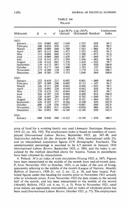
1262 JOURNAL OF POLITICAL ECONOMY
TABLE A4 POLAND
Log (MIP)t Log (M/P)t Employment Midmonth Pt aTt
e (Actual) (Estimated) Residual Index
1922: January . .116 0.003 .062 1.610 1.552 .058 89.3 February .100 0.026 .058 1.621 1.586 .036 90.5 March .. 099 0.089 .060 1.560 1.563 -.004 92.8 April .. 107 0.115 .066 1.473 1.525 -.052 94.3 May. . .112 0.088 .068 1.435 1.508 -.073 95.6 June. . .114 0.069 .068 1.438 1.507 -.069 97.7 July. . . . . .118 0.143 .075 1.394 1.456 -.062 98.6 August . . . .130 0.142 .083 1.378 1.410 -.032 99.7 September . .139 0.173 .093 1.370 1.350 .020 100.0 October. . .152 0.177 .104 1.400 1.293 .107 100.6 November. .173 0.289 .130 1.293 1.179 .114 100.7 December .204 0.303 .159 1.152 1.068 .084 100.0
1923: January . 252 0.419 .213 0.892 0.901 -.009 99.8 February .307 0.509 .290 0.605 0.712 -.107 98.5 March . .346 0.311 .298 0.662 0.696 -.035 98.1 April . 322 0.095 .220 0.910 0.882 .028 98.4 May. . .270 0.125 .192 0.984 0.962 .022 99.7 June . 268 0.297 .218 0.904 0.888 .016 100.9 July . . 320 0.497 .295 0.662 0.702 -.040 101.7 August . .396 0.503 .371 0.487 0.551 -.064 102.4 September . .428 0.385 .377 0.566 0.540 .026 102.9 October. . .608 1.229 .836 -0.037 -0.081 .044 102.8 November. .738 0.802 .811 -0.048 -0.054 .006 102.6 December .764 0.983 .941 -0.168 -0.188 .020 102.4
1924: January . . . .800 0.940 .940 -0.222 -0.188 -.034 100.5
price of food for a working family was used (Annuaire Statistique Hongrois, 1919-22, pp. 102, 193). The employment index is based on numbers of unem- ployed (International Labour Review, September 1925, pp. 347-48, and Statistisches Jahrbuch fur das Deutsche Reich, 1926, international table 23), and on interpolated population figures (UN Demographic Yearbook). The unemployment percentage is assumed to be 6.5 percent in January 1924 (International Labour Review, September 1925, p. 349), and the index is cal- culated by the method described above for Austria. Values in parentheses have been obtained by interpolation.
4. Poland: M is an index of note circulation (Young 1925, p. 347). Figures have been interpolated to the middle of the month from end-of-month data; P, from November 1921 to October, 1923, is an index of the cost of living, apparently referring to the middle of the month (League of Nations, Monthly Bulletin of Statistics, 1920-21, vol. 2, no. 12, p. 18, and later issues). Pub- lished figures under this heading for months prior to November 1921 actually refer to wholesale prices. From November 1923 the data relates to the second half of the month, and has been interpolated to the middle of the month (Monthly Bulletin, 1923, vol. 4, no. 11, p. 3). Prior to November 1921, retail price indices are apparently unavailable, and an index of wholesale prices has been used (International Labour Review, October 1921, p. 77). The employment

INFLATION AND DEMAND FOR MONEY 1263
index is based on numbers of unemployed (Statistisches Jahrbuch fur das Deutsche Reich, 1924/25, international table 13), and on interpolated popula- tion figures (UN Demographic Yearbook). The percentage of unemployed on September 1923 is assumed to be 3 percent, and the index is calculated by the method described above for Austria.
References
Allais, M. "A Restatement of the Quantity Theory of Money." A.E.R. 56 (December 1966):1123-57.
Bresciani-Turroni, C. The Economics of Inflation. London: Allen & Unwin, 1937.
Cagan, P. "The Monetary Dynamics of Hyperinflation." In Studies in the Quantity Theory of Money, edited by M. Friedman. Chicago: Univ. Chicago Press, 1956.
Durbin, J., and G. S. Watson. "Testing for Serial Correlation in Least Squares Regression LI." Biometrica 38 (June 1951):159-78.
Feller, W. An Introduction to Probability Theory and its Applications. Vol. 1, 3d ed. New York: Wiley, 1968.
Friedman, M. "The Quantity Theory of Money a Restatement." In Studies in the Quantity Theory of Money, edited by M. Friedman. Chicago: Univ. Chicago Press, 1956.
Hirshleifer, J. "On the Theory of Optimal Investment Decisions." J.P.E. 66 (August 1958):329-52.
Hogg, R., and A. Craig. Introduction to Mathematical Statistics. 2d ed. New York: Macmillan, 1965.
Keynes, J. M. A Tract on Monetary Reform. London: Macmillan, 1924. Miller, M. H., and D. Orr. "A Model of the Demand for Money by Firms."
Q.J.E. 80 (August 1966):413-35. Sonderhefte zur Wirtschaft und Statistik. "Zahlen zur Geldentwertung in
Deutschland 1914 bis 1923." Berlin: Hobbung, 1925. Statistisches Jahrbuch far das Deutsche Reich, 1924/25 and 1926. Berlin:
Statistisches Reichsamt, 1925, 1926. Walre de Bordes, J. van. The Austrian Crown. London: King, 1924. Young, J. P. European Currency and Finance. Vol. 2. Washington: Govern-
ment Printing Office, 1925.