INFLATION TARGETS AND THE

ZLB IN A BEHAVIORAL MODEL

Paul De Grauwe

London School of Economics

Yuemei Ji

University College London

Introduction

An inflation target too close to zero risks pushing the economy into a negative inflation territory even when mild shocks occur.

Such an outcome is generally considered to be dangerous.

During periods of deflation the nominal interest rate is likely to hit the lower zero bound.

When this happens the real interest rate cannot decline further.

The central bank loses its capacity to stimulate the economy in a recession, thereby risking prolonged recessions (Eggertson and Woodford(2003), Blanchard, et al. (2010), Ball(2014)).

This has led to proposals to increase the level of the inflation target (e.g. Blanchard, et al. (2010), Ball(2014))

Purpose of this research:

Revisiting the issue of the optimal level of the inflation target

when nominal interest rate is subject to zero lower bound

using a behavioral macroeconomic model

Standard linear DSGE models have tended to underestimate the probability of hitting the ZLB as was shown by Chung, et al., (2012).

Most of these models have led to the prediction that when the central bank keeps an inflation target of 2%, it is very unlikely for the economy to be pushed into the ZLB. (Coenen(2003), Schmitt-Grohe and Uribe(2007)).

We use same behavioral macroeconomic model to shed new light on the nature of this risk.

We now add:

rt≥0

Implications: non-normality

Model produces non-normally distributed output gaps

Excess kurtosis

Fat tails

These are produced by animal spirits

Most of the time: great moderation; market sentiments neutral

Regularly and unpredictably there is strong optimism (pessimism) that in self-fulfilling way creates boom (bust)

Two way causality output gap-animal spirits

How are these results are affected by the level of the inflation target?

We start by noting that the output gap in Figure 1 is slightly skewed to the left. (skewness = -0.66).

This skewness finds its origin in the fact that the distribution of animal spirits is also skewed to the left, i.e. there are more periods of pessimism than optimism.

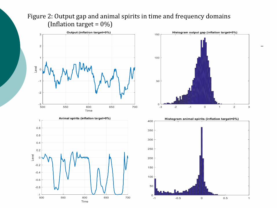
Inflation target =0%

Most of the time animal spirits are negative with many periods of extreme pessimism.

Thus when the central bank sets an inflation target equal to zero pessimism prevails most of the time

and recession is a chronic feature of the business cycle with very few periods of optimism and optimism.

Inflation target = 4%

the distribution output gap and animal spirits is symmetric.

Skewness of output gap is not statistically different from 0 and animal spirits are 0 on average.

Periods of optimism and pessimism occur equally frequently.

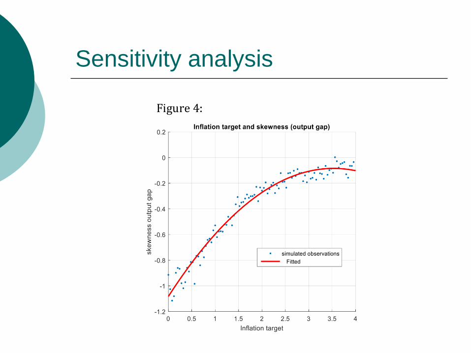
Sensitivity analysis

Interpretation

When inflation target is 0% cyclical movements in output gap and animal spirits lead to recessions that drive inflation into negative territory.

When that happens the zero bound constraint makes it impossible for the central bank to lower the real interest rate.

Chronic pessimism

If the recession is deep and deflation intense the real interest rate is likely to increase significantly.

Thus the recession becomes protracted.

Pessimism sets in and amplifies the recession, deflation and validates pessimism.

As the central bank loses its stabilizing capacity the economy gets stuck in pessimism, recession and deflation.

We conclude that an inflation target of 0% becomes a breeding ground for pessimism and recession.

The way out is to increase the inflation target.

Such an increase pulls the economy out of the chronic pessimism trap.

Our results suggest that an inflation target of 3%-4% is probably better than 2% in making sure that the economy does not get stuck in the chronic pessimism trap.

Optimal monetary policies and LZB

We construct tradeoffs between inflation and output variability

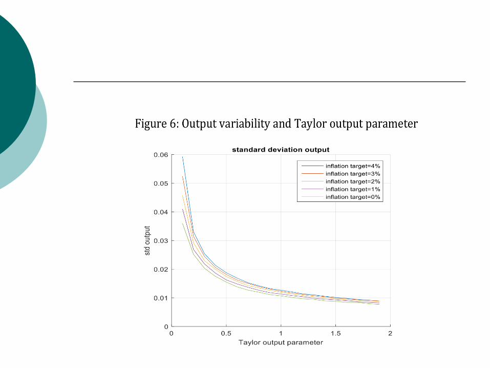
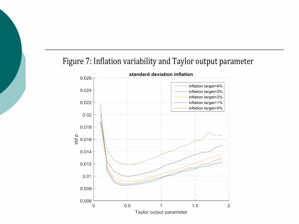
There is a range of Taylor output parameter (from 0 to 0.5) that leads to decline in both inflation and output variability

By stabilizing output the central bank also reduces the amplitude of the waves of optimism and pessimism (animal spirits) thereby stabilizing not only output but also inflation.

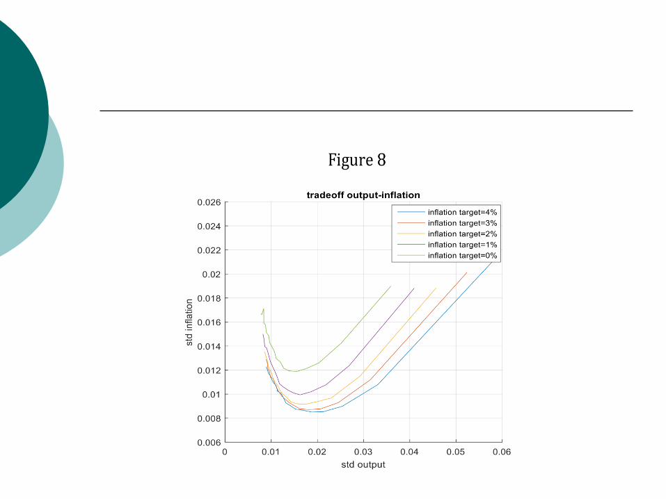
Interpretation

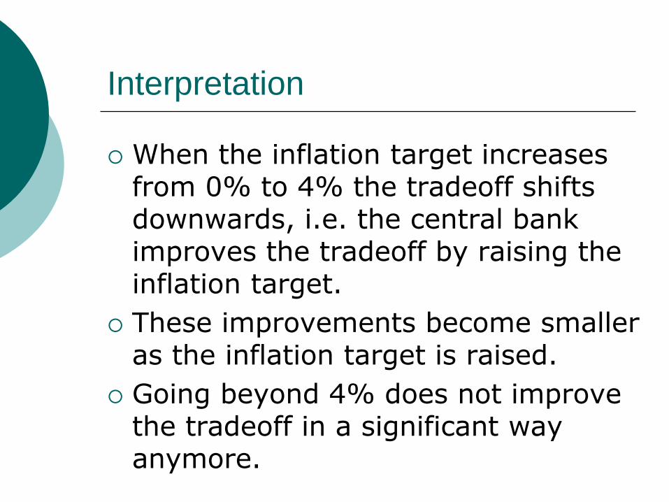
When the inflation target increases from 0% to 4% the tradeoff shifts downwards, i.e. the central bank improves the tradeoff by raising the inflation target.

These improvements become smaller as the inflation target is raised.

Going beyond 4% does not improve the tradeoff in a significant way anymore.

Credibility of inflation target and

ZLB

Model allows to define credibility in very precise way

i.e. as the fraction of agents using the announced inflation target as their forecast for inflation

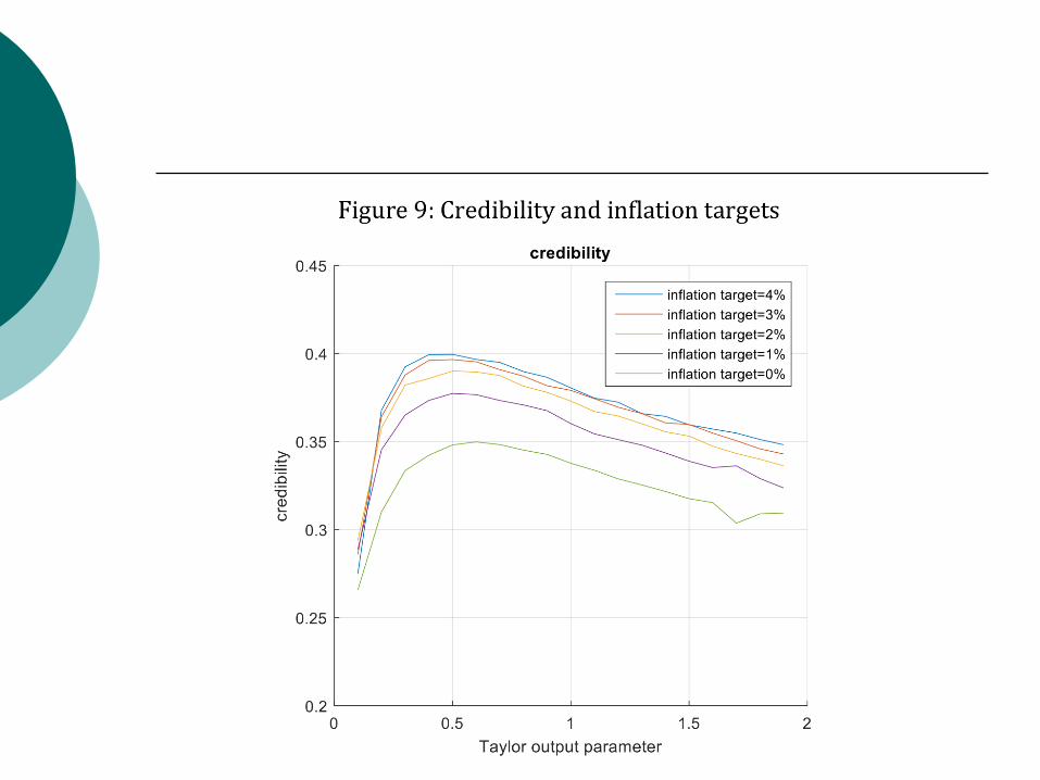
Interpretation

when the central bank increases its stabilization efforts, this has at first a positive effect on the credibility of its inflation target.

This increases its inflation credibility.

This positive effect on credibility disappears when the Taylor output parameter reaches 0.5.

It can be seen that there is a relation between the tradeoff and credibility.

Responses to

demand and supply shocks

We analyse the impulse responses to demand and supply shocks

We concentrate on the short-term effects (after 4 periods)

And represent these in frequency domain

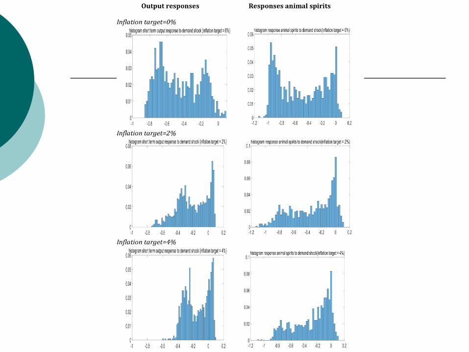
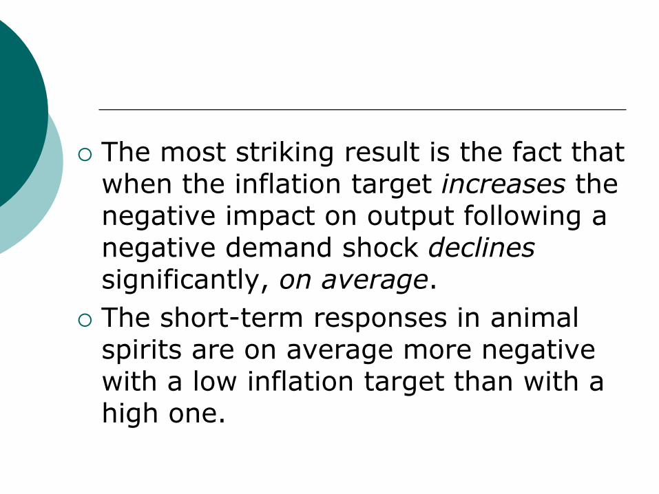
The most striking result is the fact that when the inflation target increases the negative impact on output following a negative demand shock declines significantly, on average.

The short-term responses in animal spirits are on average more negative with a low inflation target than with a high one.

But as mentioned earlier, there is a wide variation in the short-term effect of the same demand shock on output and animal spirits

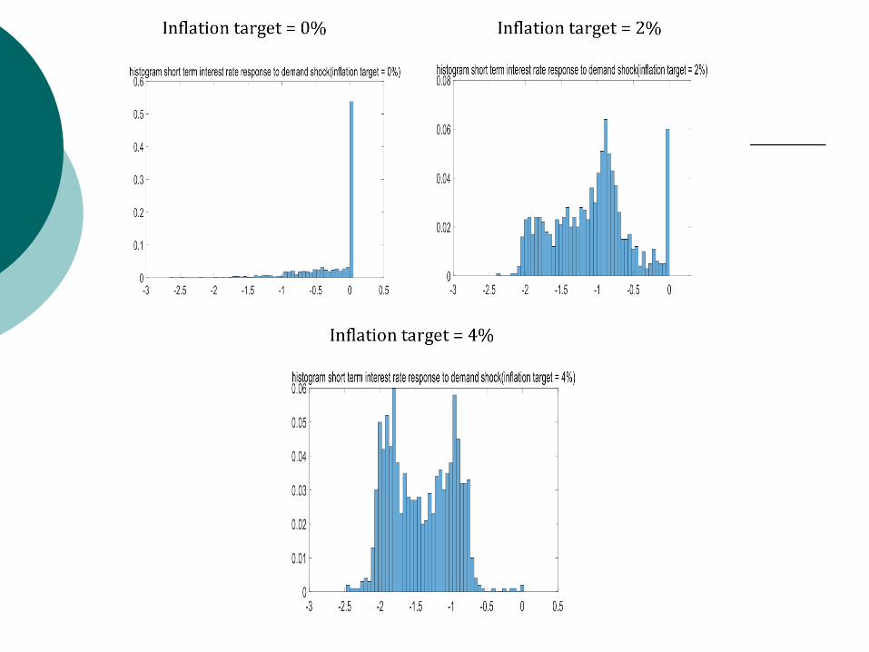
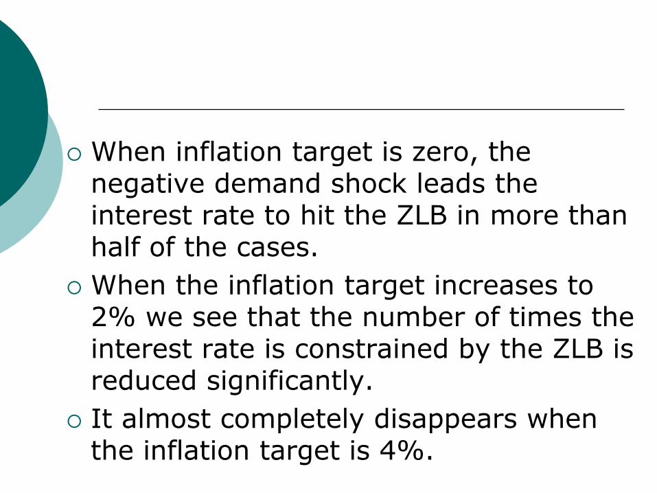
When inflation target is zero, the negative demand shock leads the interest rate to hit the ZLB in more than half of the cases.

When the inflation target increases to 2% we see that the number of times the interest rate is constrained by the ZLB is reduced significantly.

It almost completely disappears when the inflation target is 4%.

Analysis of the deterministic model

We analyze the deterministic version of the model, i.e. we strip the model of all the stochastic shocks.

This allows us to shed some light on the steady state characteristics of the model

and the speed with which the variables return to their steady state values after an initial disturbance

We assume an initial shock in demand

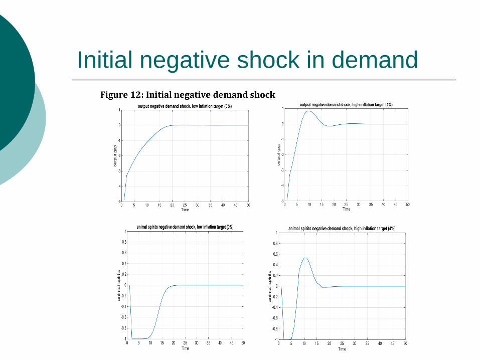
Initial negative shock in demand

Interpretation

Negative demand shock has a significantly more protracted negative effect on the output gap in the low inflation target regime as compared to the high inflation target regime.

In the low inflation target regime animal spirits are kept in negative territory longer than in the high inflation target regime.

Thus, when the central bank sets a relatively high inflation target, the capacity of the system to lift itself out of the recession is stronger than when it sets a low inflation target.

This is made possible by the stabilizing properties of monetary policies and by the ensuing elimination of self-fulfilling pessimism.

Conclusion

The use of this behavioral model has allowed us to shed new light on the optimal level of the inflation target when a lower zero bound constraint on the nominal interest rate exists.

When inflation target is too close to zero, the economy can get gripped by “chronic pessimism”

that leads to a dominance of negative output gaps and recessions,

and in turn feeds back on expectations producing long waves of pessimism.

Put differently, when the inflation target is set too close to zero the distribution of the output gap is skewed towards the negative territory.

The question is what “too close to zero” means.

The simulations of our model, using parameter calibrations that are generally found in the literature, suggests that 2% is too low, i.e. produces negative skewness in the distribution of the output gap.

We find that an inflation target in the range of 3% to 4% comes closer to producing a symmetric distribution of the output gap.

We also found that in the high inflation target regime the persistence of the recession is much shorter than in the low inflation target regime.

i.e. when the central bank sets a relatively high inflation target, the capacity of the system to lift itself out of the recession is stronger than when it sets a low inflation target.

All this leads to the conclusion that central banks should raise the inflation target from 2% to a range between 3% to 4% (see also Blanchard, et al. (2010) and Ball(2014) on this).

Extension to two countries

Introduction: Some facts II

Let us look at some facts about international correlations of business cycles

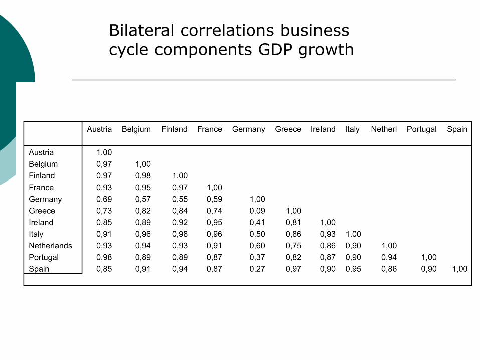
Bilateral correlations business cycle components GDP growth

Bilateral correlations business cycle components GDP growth

-20%

-15%

-10%

-5%

0%

5%

10%

15%

20%

1995 1998 2001 2004 2007 2010 2013

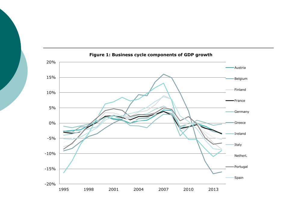
Figure 1: Business cycle components of GDP growth

Austria

Belgium

Finland

France

Germany

Greece

Ireland

Italy

NetherL

Portugal

Spain

y = 2,9541x + 0,6779

R² = 0,0617

0

0,2

0,4

0,6

0,8

1

1,2

0 0,01 0,02 0,03 0,04 0,05 0,06 0,07 0,08 0,09 0,1

Corr

ela

tion o

f busin

ess c

ycle

trade links (sum of trade/sum of GDP)

Figure 2: Correlation of business cycle and trade links in 11 Eurozone

countries

y = 8,7112x + 0,5852

R² = 0,0472

-0,2

0

0,2

0,4

0,6

0,8

1

1,2

0 0,005 0,01 0,015 0,02 0,025 0,03 0,035 0,04 0,045

Corr

ela

tion o

f busin

ess c

ycle

Trade links (sum of export/sum of GDP)

Figure 3: Correlation of business cycle and trade links in 12 stand-alone

countries

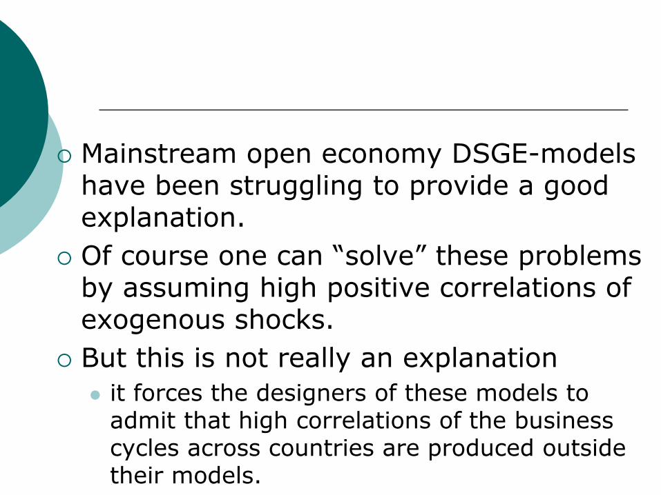
Mainstream open economy DSGE-models have been struggling to provide a good explanation.

Of course one can “solve” these problems by assuming high positive correlations of exogenous shocks.

But this is not really an explanation

it forces the designers of these models to admit that high correlations of the business cycles across countries are produced outside their models.

There have been attempts to explain the high synchronization of the business cycles across countries by introducing financial integration in the models

This goes some way in explaining this synchronization.

But again too much is “explained” by introducing highly correlated exogenous financial shocks.

A behavioral model approach

We want to go further

And make the explanation endogenous in the model

i.e. not having to rely exclusively on correlation of exogenous shocks across countries

Monetary union model

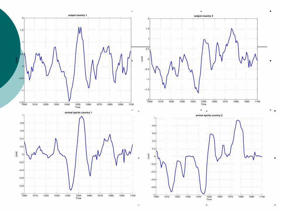
Frequency distribution output gap and animal spirits

Implications: international contagion

Model produces international contagion of animal spirits.

Animal spirits are highly correlated between the two countries reaching 0.95.

Why? When a wave of optimism is set in motion in country 1, it leads to more output and imports in that country, thereby increasing output in country 2.

Positive transmission, even if small, makes it more likely that agents in country 2 that make optimistic forecasts are vindicated, thereby increasing the fraction of agents in country 2 that become optimists.

We obtain transmission dynamics that triggered by trade flows is amplified leading to strong synchronization of the business cycles across countries.

Similar result in model with monetary independence

Correlation is non-linear

-1

-0,8

-0,6

-0,4

-0,2

0

0,2

0,4

0,6

0,8

11 7

13

19

25

31

37

43

49

55

61

67

73

79

85

91

97

103

109

115

121

127

133

139

145

151

157

163

169

175

181

187

193

199

Figure 30: Animal spirits in country 1 and 2

country 1

country 2

Implications

International correlation of business cycles is dominated by extreme movements in animal spirits

Extreme optimism gets easily propagated internationally

The same is true with extreme pessimism

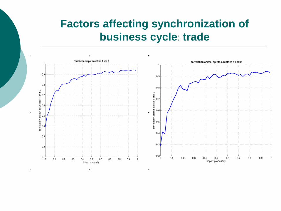
Factors affecting synchronization of

business cycle: trade

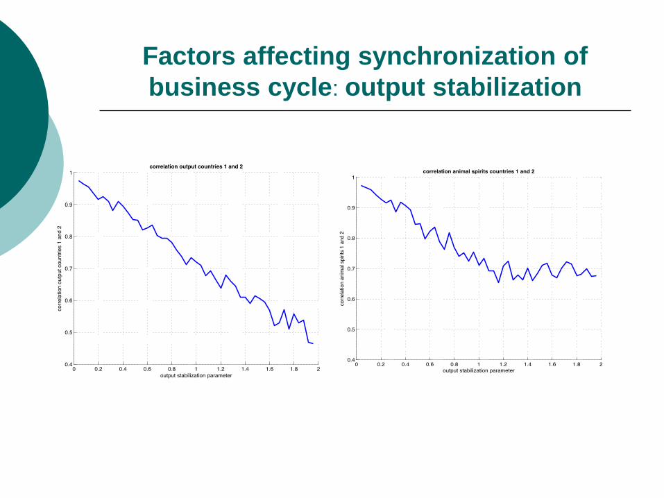
Factors affecting synchronization of

business cycle: output stabilization

Conclusion

Main channel of international synchronization business cycles occurs through a propagation of “animal spirits”,

i.e. waves of optimism and pessimism that get correlated internationally.

this propagation occurs with relatively low levels of trade integration.

and is more intense when optimism and pessimism are extreme

Degree of synchronization is influenced by the intensity with which the central bank stabilizes output.

Empirical Issues

Introduction

A theoretical model can only convince if it passes some form of empirical testing.

This is also the case with the behavioural model discussed in these lectures.

The problem in macroeconomics is how to devise a credible empirical test of the model.

The history of macroeconomics is littered with examples of models which passed econometric testing procedures with flying colors, to be found wanting later. The DSGE-models are no exceptions to this rule.

I will follow the approach of indirect inference, i.e. I ask the question what the predictions of the theoretical model are and confront these predictions with the data.

Of course, it should be stressed from the start that a lot of uncertainty will continue to prevail about the empirical validity of the behavioural model.

Main predictions of the

behavioural model.

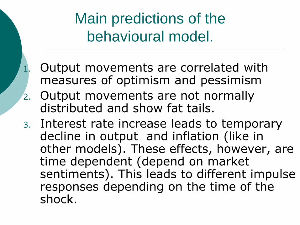
1. Output movements are correlated with

measures of optimism and pessimism

2. Output movements are not normally distributed and show fat tails.

3. Interest rate increase leads to temporary decline in output and inflation (like in other models). These effects, however, are time dependent (depend on market sentiments). This leads to different impulse responses depending on the time of the shock.

Correlation output movements and

animal spirits

• Concept of animal spirits, i.e. waves of optimism and pessimism, plays a central role in our model

• Is there an empirical counterpart for this concept?

• There is one: Many countries use survey based consumer and/or business sentiment indicators as a tool of analyzing the business cycle and as a predictive instrument.

• How well do these indicators correlate with output movements? 73

74

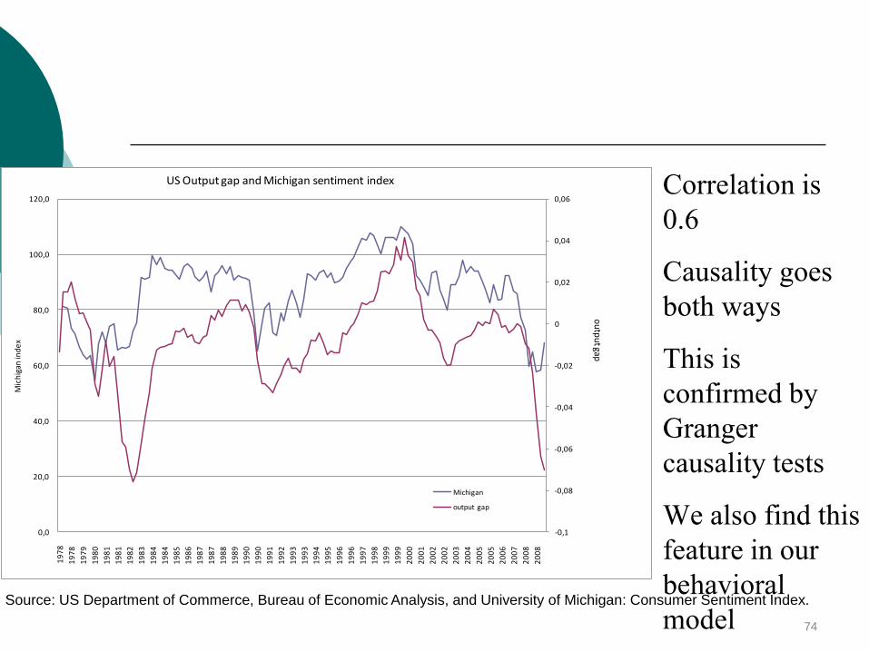
Source: US Department of Commerce, Bureau of Economic Analysis, and University of Michigan: Consumer Sentiment Index.

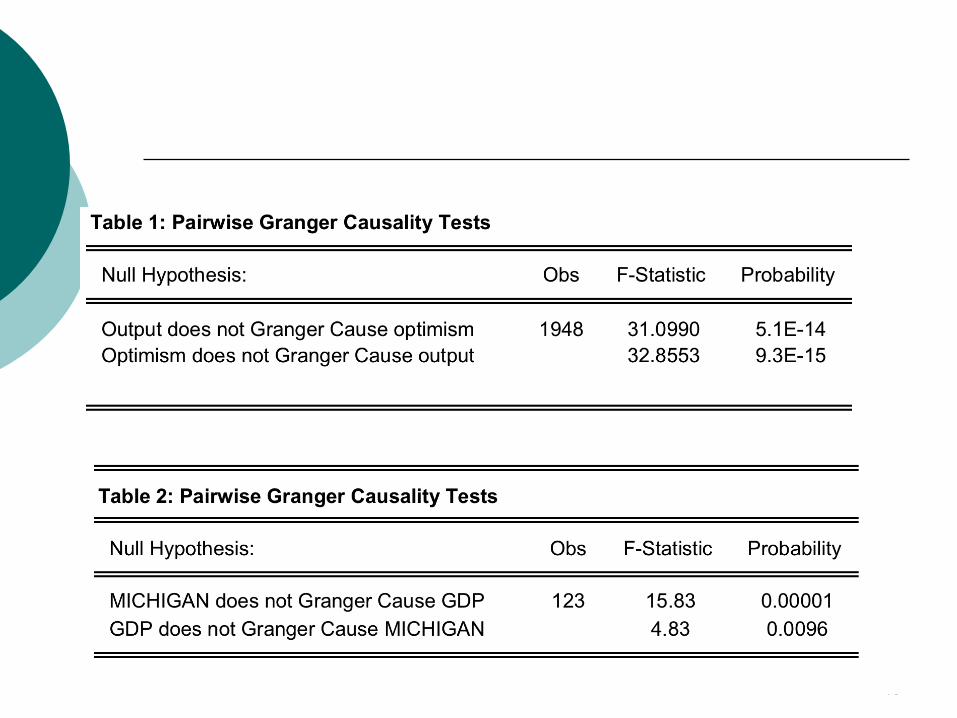
Correlation is

0.6

Causality goes

both ways

This is

confirmed by

Granger

causality tests

We also find this

feature in our

behavioral

model

-0,1

-0,08

-0,06

-0,04

-0,02

0

0,02

0,04

0,06

0,0

20,0

40,0

60,0

80,0

100,0

120,0

19

78

19

78

19

79

19

80

19

81

19

81

19

82

19

83

19

84

19

84

19

85

19

86

19

87

19

87

19

88

19

89

19

90

19

90

19

91

19

92

19

93

19

93

19

94

19

95

19

96

19

96

19

97

19

98

19

99

19

99

20

00

20

01

20

02

20

02

20

03

20

04

20

05

20

05

20

06

20

07

20

08

20

08

Mic

hig

an in

de

x

US Output gap and Michigan sentiment index

Michigan

output gap

ou

tpu

t gap

75

Model predictions: higher moments

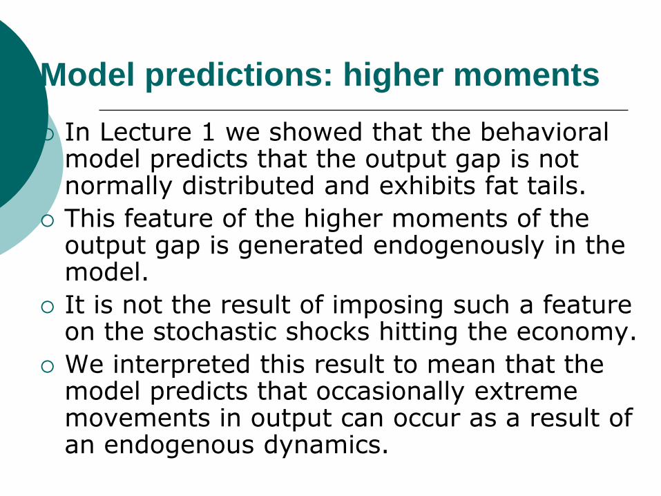
In Lecture 1 we showed that the behavioral model predicts that the output gap is not normally distributed and exhibits fat tails.

This feature of the higher moments of the output gap is generated endogenously in the model.

It is not the result of imposing such a feature on the stochastic shocks hitting the economy.

We interpreted this result to mean that the model predicts that occasionally extreme movements in output can occur as a result of an endogenous dynamics.

We already confronted this prediction with data from the US and concluded that indeed the distribution of the US output gap during the postwar period was not normal.

We now look at other countries, i.e. the UK and Germany. Unfortunately the sample period is shorter and only starts in 1990.

For the sake of comparability we also present the US data for this shorter period.

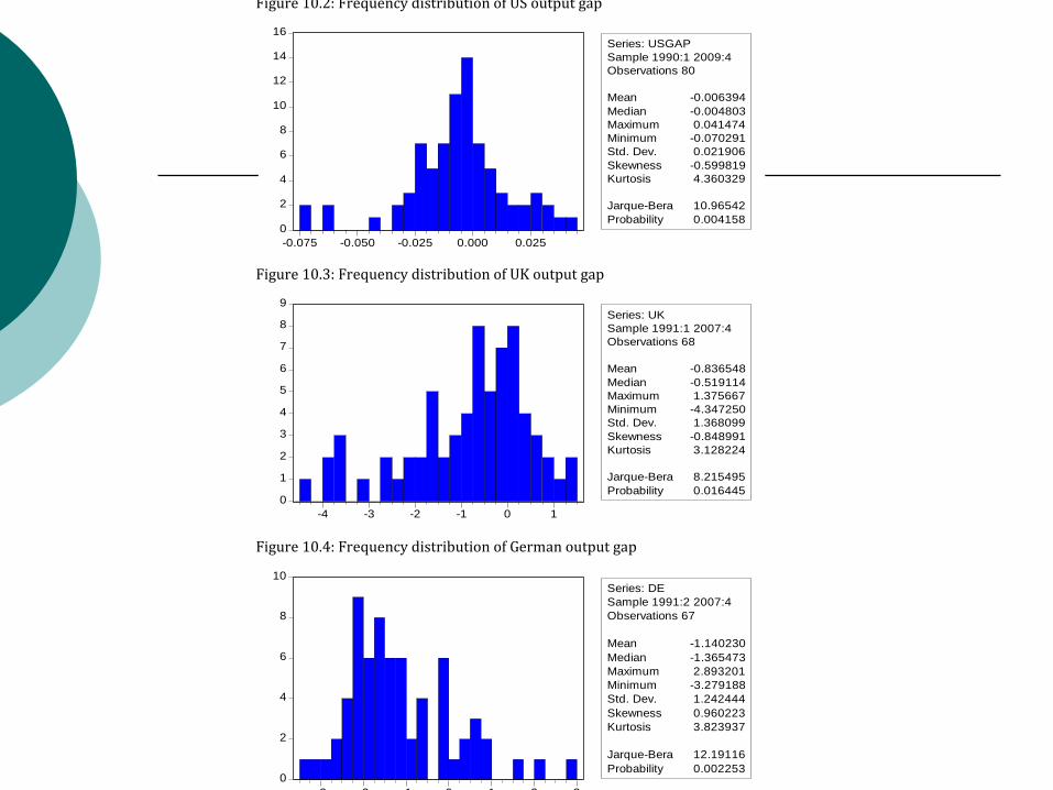
Figure10.2:FrequencydistributionofUSoutputgap

Figure10.3:FrequencydistributionofUKoutputgap

Figure10.4:FrequencydistributionofGermanoutputgap

0

2

4

6

8

10

12

14

16

-0.075 -0.050 -0.025 0.000 0.025

Series: USGAP

Sample 1990:1 2009:4

Observations 80

Mean -0.006394

Median -0.004803

Maximum 0.041474

Minimum -0.070291

Std. Dev. 0.021906

Skewness -0.599819

Kurtosis 4.360329

Jarque-Bera 10.96542

Probability 0.004158

0

1

2

3

4

5

6

7

8

9

-4 -3 -2 -1 0 1

Series: UK

Sample 1991:1 2007:4

Observations 68

Mean -0.836548

Median -0.519114

Maximum 1.375667

Minimum -4.347250

Std. Dev. 1.368099

Skewness -0.848991

Kurtosis 3.128224

Jarque-Bera 8.215495

Probability 0.016445

0

2

4

6

8

10

-3 -2 -1 0 1 2 3

Series: DE

Sample 1991:2 2007:4

Observations 67

Mean -1.140230

Median -1.365473

Maximum 2.893201

Minimum -3.279188

Std. Dev. 1.242444

Skewness 0.960223

Kurtosis 3.823937

Jarque-Bera 12.19116

Probability 0.002253

Transmission of monetary policy

shocks

Empirical testing in macroeconomics has been very much influenced by Sims(1980) seminal contribution.

The basic idea is that theoretical models make predictions about the effects of policy shocks and that these predictions can be confronted with the data.

The way this can be done is to estimate a VAR of the macroeconomic variables and the policy variable.

In the context of our model this consists in estimating a VAR of inflation, output gap and the interest rate.

This VAR then allows to estimate an impulse response of inflation and output gap on interest rate shocks.

This impulse response obtained from the data is then compared with the impulse response predicted by the theoretical model.

It is important that, in doing so, the empirical impulse response is theory-free, i.e. does not use theory to impose identifying restrictions.

In practice, this is not always easy to do, because restrictions on the parameters of the VAR must be imposed to be able to identify the impulse responses.

The condition therefore has been to impose restrictions that use the least possible theory, or put differently, that are used in the largest possible class of theoretical model.

The Choleski decomposition is generally considered as the most theory-free set of restrictions.

We now confront the theoretical impulses obtained from our behavioral model with the empirical ones.

As a first step, we estimated a VAR-model with three variables (output, inflation and short term interest rate) for the US, using a Choleski decomposition (with ordering of inflation, output, interest rate).

We then computed the impulse responses of output to an increase in the short-term interest rate (the Federal Funds rate).

One of the main predictions of the behavioral model is that the impulse responses are very much influenced by the timing of the shock.

We tested the empirical validity of this prediction by computing different impulse responses over different sample periods.

We allowed for rolling sample periods of 30 years starting in 1972, and moving up each month.

For each of these sample periods we computed the shot-term output effect of an increase in the Federal Fund rate, where short-term refers to the effect after one year.

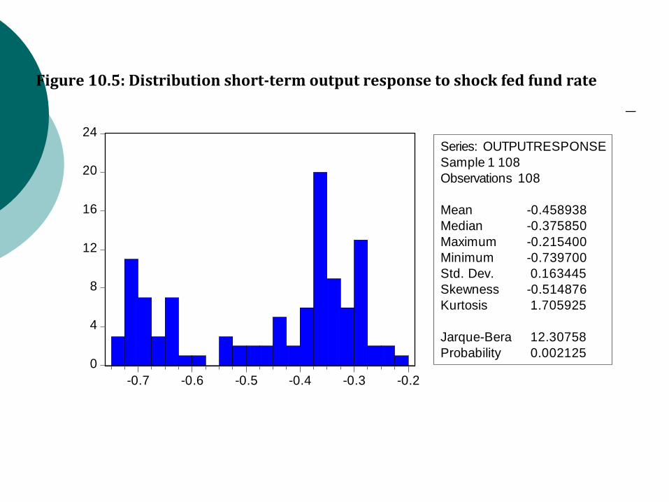
Figure10.5:Distributionshort-termoutputresponsetoshockfedfundrate

0

4

8

12

16

20

24

-0.7 -0.6 -0.5 -0.4 -0.3 -0.2

Series: OUTPUTRESPONSE

Sample 1 108

Observations 108

Mean -0.458938

Median -0.375850

Maximum -0.215400

Minimum -0.739700

Std. Dev. 0.163445

Skewness -0.514876

Kurtosis 1.705925

Jarque-Bera 12.30758

Probability 0.002125

We find a wide range of short-tem effects to the same policy shock (between -0.2% and -0.7% for a 1 standard deviation shock in the interest rate).

In addition, we find that the distribution of theses output responses is not normal. The Jarque-Bera test overwhelmingly rejects normality.

empirical results confirm the theoretical prediction of the behavioral model, i.e. the timing of the shock matters a great deal and affects how the same policy shock is transmitted into the economy.

In addition, the non-normality in the distribution of these shocks transforms risk into uncertainty.

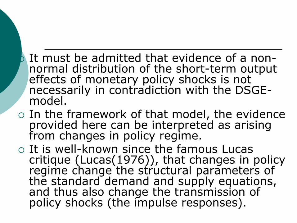
It must be admitted that evidence of a non-normal distribution of the short-term output effects of monetary policy shocks is not necessarily in contradiction with the DSGE-model.

In the framework of that model, the evidence provided here can be interpreted as arising from changes in policy regime.

It is well-known since the famous Lucas critique (Lucas(1976)), that changes in policy regime change the structural parameters of the standard demand and supply equations, and thus also change the transmission of policy shocks (the impulse responses).

In this interpretation, the evidence of non-normal distribution of the short-term output effects of a monetary policy shock is consistent with the view that there have been different changes in the policy regime during the sample period.

These changes then produce non-normal distributions of these effects.

Again we have two radically different interpretations of the same empirical evidence (which is not unusual in economics).

However, interpretation given in the behavioral model is simpler than the one provided in the DSGE-model.

In the latter, the theoretical model predicts that provided the policy regime does not change, a policy shock will always have the same effect.

With noise in the data, the estimated effects of these shocks should be normally distributed.

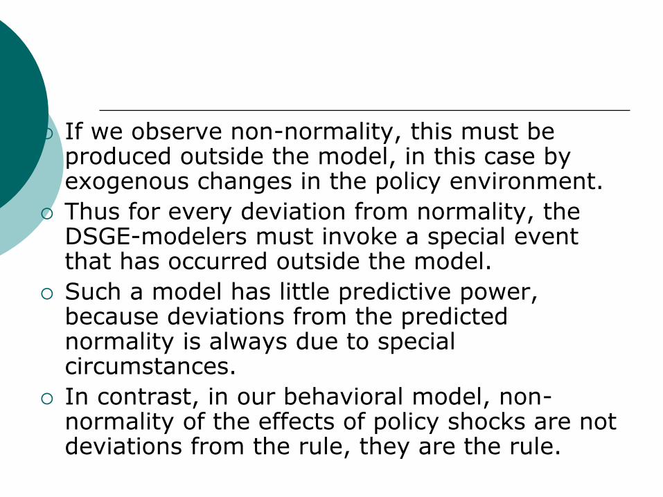
If we observe non-normality, this must be produced outside the model, in this case by exogenous changes in the policy environment.

Thus for every deviation from normality, the DSGE-modelers must invoke a special event that has occurred outside the model.

Such a model has little predictive power, because deviations from the predicted normality is always due to special circumstances.

In contrast, in our behavioral model, non-normality of the effects of policy shocks are not deviations from the rule, they are the rule.