Inflation in the G7: Mind the Gap(s)? *

James Morley

Washington University in St. Louis

Jeremy Piger University of Oregon

Robert Rasche

Federal Reserve Bank of St. Louis

April 2, 2010

PRELIMINARY: PLEASE DO NOT CITE WITHOUT AUTHORS’ PERMISSION ABSTRACT: We investigate the relative importance of trend inflation, the real-activity gap, and supply shocks for explaining observed inflation variation in G7 countries over the post-war period. Our results are based on a bivariate unobserved-components model of inflation and unemployment in which inflation is decomposed into a stochastic trend and a transitory component. As in recent implementations of the New Keynesian Phillips Curve, it is the transitory component of inflation, or “inflation gap”, that is driven by the real activity gap, which we measure as the deviation of unemployment from its natural rate. We find that both trend inflation and the inflation gap have been important determinants of actual inflation variation for most countries. Also, the real-activity gap explains a significant amount of the variation in the inflation gap for Canada and the European countries in our sample, suggesting the New Keynesian Phillips Curve, once augmented to include trend inflation, is an empirical success for these countries. However, for the U.S. and Japan, the real-activity gap explains only a small amount (less than 10%) of the variation in the inflation gap. We also provide new estimates of trend inflation for the G7 countries that incorporate information in the real-activity gap for identification and, through formal model comparisons, new statistical evidence regarding structural breaks in the variability of trend inflation. Keywords: inflation gap, inflation persistence, natural rate, Phillips Curve, trend inflation JEL Classification: C32, E31, E32

* Morley: Department of Economics, Box 1208, Eliot Hall 205, Washington University, One Brookings Drive, St. Louis, MO 63130, (morley@wustl.edu); Piger: Department of Economics, 1285 University of Oregon, Eugene, OR 97403 (jpiger@uoregon.edu); Rasche: Research Department, Federal Reserve Bank of St. Louis, P.O. Box 442, St. Louis, MO 63166 (rasche@stls.frb.org). Portions of this research were completed while Morley and Piger were visitors to the Federal Reserve Bank of St. Louis. The views expressed here are those of the authors and do not necessarily reflect official positions of the Federal Reserve Bank of St. Louis, the Federal Reserve System, or the Board of Governors.

1

Introduction

The Phillips Curve is one of the most recognizable theoretical constructs in

macroeconomics. In its modern form, the Phillips Curve relates observed inflation to expected

inflation and a measure of excess demand, where the latter is most commonly expressed as the

gap between the actual and potential levels of real activity. This assumed relationship between

inflation and the “real-activity gap” is a primary link through which monetary policy affects the

inflation rate in contemporary monetary models.

Despite its theoretical appeal, the empirical evidence linking the real-activity gap to

inflation is mixed. A large literature, typified by the work of Robert Gordon (1982, 1997, 1998),

estimates Phillips Curve equations for which the expected inflation term is replaced by lags of

inflation. In the so-called “accelerationist” version of this model, the coefficients on lagged

inflation are constrained to sum to unity. Such “backward looking” implementations of the

Phillips Curve typically find that the real-activity gap, whether measured using output or the

unemployment rate, is strongly statistically significant as a driver for U.S. inflation. However, if

one instead assumes rational expectations, as in the “New Keynesian” version of the Phillips

Curve (NKPC), the evidence in favor of the real-activity gap as an inflation driver is lessened. A

number of studies, including Fuhrer and Moore (1995), Fuhrer (1997), Roberts (2001), and

Estrella and Fuhrer (2002), find that the estimated effect of the real-activity gap in NKPC

equations for U.S. inflation is insignificant, and in some cases has a counterintuitive sign.1

Another empirical shortcoming of the NKPC relates to its inability to generate substantial

inflation persistence. The NKPC implies that inflation is a discounted present value of expected

1 In the NKPC, the theoretical driving variable for inflation is real marginal cost, which is then proxied for with the real-activity gap. Gali and Gertler (1999) and Gali, Gertler, and Lopez Salido (2001) consider an alternative proxy, the average labor share of national income, and report a better fit for modeling U.S and Euro area inflation rates. However, use of the average labor share as a proxy for real marginal cost is not without criticism (see, e.g., Rudd and Whelan, 2005).

2

real-activity gap terms, which, assuming the real-activity gap is covariance stationary, implies

that inflation itself is covariance stationary. Further, estimates of the discounted present value of

expected gap terms display low levels of persistence. This is counterfactual, as it is difficult to

reject the null hypothesis of a unit root for the inflation rates of many countries. Indeed, it is now

standard for univariate statistical characterizations of inflation to include a stochastic trend.2 In

response to this, recent contributions, including Cogley and Sbordone (2008) and Goodfriend

and King (2009), augment the NKPC to allow for trend inflation. In these models, it is the

“inflation gap”, or the difference between inflation and its trend, that is influenced by the real-

activity gap. Empirical implementations of the NKPC with trend inflation provide more evidence

in favor of the real-activity gap as an inflation driver. For example, Lee and Nelson (2007),

Harvey (2008), Piger and Rasche (2008), and Manopimoke (2010) find that the real-activity gap

is a statistically significant driver of the U.S. inflation gap, while Cogley and Sbordone (2008)

find that the fit of the NKPC for the inflation gap is improved over that for inflation itself.

However, Piger and Rasche (2008) note that despite the statistical significance of the real-

activity gap, it accounts for a relatively small fraction of the variation in observed U.S. post-war

inflation as compared to that contributed by the inflation trend.

In this paper, we provide evidence regarding the relative importance of trend inflation,

the real-activity gap, and supply shocks for explaining inflation variation in the G7 economies.

We work with a bivariate unobserved-components (UC) model of inflation and unemployment

that is a reduced form of the NKPC with trend inflation. The real-activity gap is measured as the

deviation of unemployment from its natural rate, where, as in Staiger, Stock and Watson (1997)

and Laubach (2001), the natural rate is equal to the stochastic trend in unemployment. The real-

2 Stock and Watson (2007) and Kang, Kim and Morley (2010) estimate univariate models in which U.S. inflation is decomposed into stochastic trend and cyclical components. Cecchetti, et al. (2007) applies the Stock and Watson (2007) model to G7 inflation data.

3

activity gap is assumed to drive the inflation gap, measured as the deviation of actual and trend

inflation. Following a large recent literature, for example Stock and Watson (2007), we measure

trend inflation using the stochastic trend in inflation and allow for instability, in the form of

multiple discrete structural breaks of unknown timing, in the variance of shocks to this stochastic

trend. The model is estimated using a Bayesian framework, and posterior probabilities used to

formally compare models with alternative numbers and types of structural breaks.

The bivariate UC model is fit to the inflation rates of the G7 countries over sample

periods that range from the past 30-50 years depending on country. The estimation results

suggest that both the inflation trend and the inflation gap have been important drivers of actual

inflation for most countries over these sample periods. In particular, the inflation trend and

inflation gap have contributed significantly to the variation of actual inflation changes at various

horizons ranging from one quarter to six years. The primary exception is Germany, for which the

inflation trend has contributed only small amounts to the variability of actual inflation changes

over all horizons considered. Turning to the determinants of the inflation gap, the results suggest

very significant differences in the importance of the real-activity gap for explaining variation in

the inflation gap. For some countries, most notably Canada and the United Kingdom, the

variation in the real-activity gap explains more than 50% of the variation in the inflation gap. For

others, most notably Japan and the United States, the real-activity gap explains less than 10% of

the variability in the inflation gap. Overall, the results suggest that the NKPC with trend inflation

is an empirical success for many of the G7 economies, in that the real-activity gap explains a

substantial portion of the variation in the inflation gap. Notably however, the United States is not

one of these countries.

4

The results also produce new estimates of trend inflation for the G7 economies, as well as

shed new light on the possible presence of structural changes in the variance of shocks to trend

inflation. For most countries considered, the level of trend inflation has varied substantially over

time, and has drifted downward in recent decades to be near historical lows at the end of the

sample period. Again, German inflation is an exception to this pattern, with estimated trend

inflation that shows no perceptible drift. For many countries, the level of trend inflation has been

on average above actual inflation for significant periods in the 1980s and 1990s, which is driven

by unemployment rates that are above the estimated natural rate. This result highlights the

information that the real-activity gap adds for identification of trend inflation. Finally, the model

comparisons find strong evidence of structural breaks in the variance of shocks to trend inflation

for France, Japan, the United States, and the United Kingdom, but little evidence of breaks for

Canada, Germany and Italy. For all countries considered, the volatility of shocks to trend

inflation is near historical lows at the end of the sample period.

As trend inflation in our model represents the permanent variation in inflation, it is

closely tied to long-horizon expectations of inflation. Indeed, as in Beveridge and Nelson (1981),

the long-run expectation of inflation at time t is equivalent to the expectation of trend inflation

formed using time t information. Thus, our results could alternatively be interpreted as

suggesting that long-horizon inflation expectations have played an important, although not

dominant, role in explaining inflation variation in most G7 countries, and that long-horizon

expectations are currently “anchored” at low levels across the G7. This recent similarity exists

despite differences in monetary institutions across G7 countries, primarily the choice of whether

or not the monetary authority will formally adopt inflation targeting.

5

Our paper is most closely related to several recent studies of inflation dynamics that

incorporate trend inflation. Lee and Nelson (2007), Harvey (2008), Piger and Rasche (2008), and

Manopimoke (2010) estimate similar bivariate UC models of inflation and unemployment and

investigate the statistical significance of the real-activity gap. However, they do not consider data

outside the United States. Cecchetti, Hooper, Kasman, Schoenholtz, and Watson (2007), estimate

a UC model that separates each G7 inflation series into a stochastic trend plus a cycle, and allow

for time variation in the variance of shocks to the inflation trend. However, these authors focus

on univariate analysis in which the cyclical component of inflation is not influenced by the real

activity gap, and so do not provide evidence regarding the relative importance of the real-activity

gap for explaining inflation variation in the G7. Also, we find that incorporating information

from the real-activity gap for identification of trend inflation makes for significant differences in

the estimated pattern of trend inflation in several countries. Finally, these authors do not conduct

formal testing or model comparisons regarding the statistical importance of parameter changes.

For most countries, our results confirm those in Cecchetti et al. (2007) regarding the pattern of

structural change, providing additional statistical support for their findings. For others, most

notably Canada, our results support a different pattern of change from that documented in

Cecchetti et al. (2007).

The remainder of this paper is organized as follows. Section 2 motivates and details the

bivariate UC model used in our analysis. Section 3 discusses the G7 inflation data, and describes

the Bayesian techniques we use for estimation and model comparison. Section 4 presents the

results and discusses possible implications. Section 5 concludes.

6

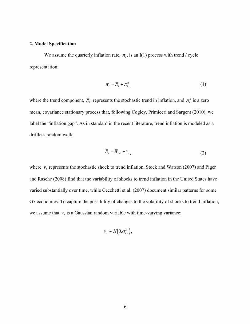
2. Model Specification

We assume the quarterly inflation rate,

€

π t , is an I(1) process with trend / cycle

representation:

€

π t = π t +π tg, (1)

where the trend component,

€

π t , represents the stochastic trend in inflation, and

€

π tg is a zero

mean, covariance stationary process that, following Cogley, Primiceri and Sargent (2010), we

label the “inflation gap”. As in standard in the recent literature, trend inflation is modeled as a

driftless random walk:

€

π t = π t−1 + vt , (2)

where

€

vt represents the stochastic shock to trend inflation. Stock and Watson (2007) and Piger

and Rasche (2008) find that the variability of shocks to trend inflation in the United States have

varied substantially over time, while Cecchetti et al. (2007) document similar patterns for some

G7 economies. To capture the possibility of changes to the volatility of shocks to trend inflation,

we assume that

€

vt is a Gaussian random variable with time-varying variance:

€

vt ~ N 0,σv,t2( ) ,

7

where

€

σv,t2 follows a discrete structural break process with m structural changes. That is,

€

σv,t2 =σv,i

2 ,

€

i =1,...,m +1. In the empirical implementation of the model, we treat the selection of m

as a problem of model selection.3

The trend inflation component has strong links to the long-horizon forecast of inflation,

which is equivalent to “core inflation” as defined by Bryan and Cecchetti (1994). Since

€

π tg is

covariance stationary with zero mean, and

€

π t follows a random walk, the long horizon inflation

expectation can be written as:

€

limh→∞

Et π t+h( ) = Et π t( ),

where

€

Et is an expectation formed using information available at time t. Thus, the minimum

mean-squared error estimate of trend inflation at time t is equivalent to the long-horizon forecast

of inflation arising from the model. Also, as discussed in Bernanke (2007), since trend inflation

in the model captures permanent changes to the inflation rate, it is unlikely that trend inflation

would display substantial variation that wasn’t mirrored in long-horizon forecasts of inflation.

Finally, several studies, including Cecchetti et al. (2007), Clark and Davig (2008) and Piger and

Rasche (2008) show that survey measures of long-horizon inflation expectations are closely

aligned with estimates of trend inflation in the United States.

The modern Phillips Curve posits a short-run tradeoff between inflation and the real-

activity gap. In our framework, this suggests that the real-activity gap should be a driver of the

inflation gap, which represents the temporary deviation of inflation from its stochastic trend. To

3 Stock and Watson (2007) and Cecchetti et al. (2007) model the variance of the innovation to trend inflation as following a stochastic volatility process, where the change to the variance is a stochastic shock that comes from a high or low volatility regime. In the implementation of their model, they fix the probability of the high volatility regime to be small, suggesting that large changes to the volatility of trend inflation occur only infrequently. Thus, their model is not inconsistent with the structural break model that we employ here.

8

capture this, we specify the following linear relationship between the inflation gap and the real-

activity gap:

€

π tg = δ j

j=0

px

∑ xt− j + γ jj=0

pz

∑ zt− j +ω t , (3)

€

ω t ~ N 0,σω2( ) .

In (3),

€

π tg is partially determined by a distributed lag of the real-activity gap, denoted

€

xt . As is

common in the Phillips Curve literature, we augment (3) with a measure of supply shocks,

denoted

€

zt , which is thought to temporarily change the level of inflation. Section 3 discusses the

choice of

€

zt that we use in estimation. The term

€

ω t is an irregular component added for

econometric implementation of the model.

We measure the real-activity gap as the deviation of the unemployment rate from its

natural rate. In particular, and similarly to inflation, we assume that the quarterly unemployment

rate is an I(1) process with a trend / cycle representation:

€

ut = u t + xt . (4)

Following Staiger, Stock and Watson (1997) and Laubach (2001), we assume that the natural

rate,

€

u t , is equivalent to the stochastic trend in the unemployment rate, modeled as a driftless

random walk:4

€

u t = u t−1 +ηt , (5)

€

ηt ~ N 0,ση2( ).

4 Laubach (2001) finds that a random walk with time-varying drift is the preferred process for the natural rate in several G7 countries. We plan to investigate this alternative specification in future drafts.

9

Finally, the real activity gap is modeled as an autoregressive process:

€

φ L( )xt = ε t , (6)

€

ε t ~ N 0,σε2( ) ,

where

€

φ L( ) is an invertible qth-order lag polynomial.

Taken together, equations (1)-(6) form a bivariate UC model for inflation and

unemployment. As discussed in Harvey (2008) and Manopimoke (2010), this model can be

interpreted as the reduced form of the NKPC with trend inflation described in Goodfriend and

King (2009). In particular, the NKPC with trend inflation implies that the inflation gap has the

following dynamics:

€

π tg = κ β j Et xt+ j( )

j=0

∞

∑ , (7)

where

€

β is the discount rate. Assuming that

€

xt follows an autoregressive process as in (6), the

expectations in (7) have a simple, recursive, structure that yields a linear expression for

€

π tg in

terms of current and lagged values of the real-activity gap. For example, if

€

xt = φxt−1 +ε t , then

we have the following reduced form for (7) upon substituting expectations:

€

π tg = δxt ,

€

δ =κ

1− βφ.

Thus, the inflation gap equation in (3) is a reduced form of (7), augmented to include a role for

supply shocks (

€

zt) and an irregular component (

€

ω t ).

10

The model in (1)-(6) also has connections to the accelerationist version of backward-

looking Phillips Curve models. In these models, inflation dynamics are described by:

€

π t = α jπ t− jj=1

pπ

∑ + δ j xt− jj=0

px

∑ + γ j zt− jj=0

pz

∑ +ω t , (8)

where

€

α jj=1

pπ

∑ =1. As discussed in Harvey (2008) and Piger and Rasche (2008), equations (1)-(3)

above result from replacing the lags of inflation in (8) with the trend inflation component in (2).

However, while related, these models have significant differences in their implications for

inflation dynamics. In particular, in the accelerationist Phillips Curve, inflation persistence is a

structural feature of the model, in that all variation in inflation becomes mechanically imbedded

in the permanent component of inflation. By contrast, in the model in (1)-(6), only events that

influence the shock to trend inflation have permanent effects. Further, Stock and Watson (2007)

and Cecchetti at al. (2007) present evidence that the first difference of G7 inflation series contain

important moving average dynamics. The additive structure of the trend / cycle decomposition in

(1) generates such dynamics, regardless of the influence of the real-activity gap or supply shocks.

3. Data and Estimation

We estimate the bivariate UC model in (1)-(6) for each of the G7 countries, which

requires data on inflation (

€

π t), the unemployment rate (

€

ut), and a measure of supply shocks (

€

zt)

for each country. To measure the inflation rate, we use the log first difference, multiplied by 400,

of the quarterly consumer price index of each country. As a measure of supply shocks, we use

food and energy price inflation for each country, measured as the difference between total

11

inflation and the inflation rate of the CPI excluding food and energy prices.5 All data was

obtained from the OECD database. For each country, we use data for the longest date range for

which all three variables are available, which differed substantially across countries. Data for the

United States, United Kingdom, and Canada begins in the late 1950s or early 1960s, for Japan in

1970, and for France, Germany and Italy in the late 1970s or early 1980s. Table 1 details the

exact sample periods used in estimation for each country.

We have identified a few specific cases in which exogenous events, such as shifts in VAT

or other sales tax rates, resulted in large transitory fluctuations in the inflation series. The dates

of these events are listed in Table 2. So as not to allow such outliers to dominate our results

regarding the contribution of the transitory component of inflation to the inflation process, we

replace these outliers with interpolated values (the median of the six adjacent observations that

were not themselves outlier observations).

The bivariate UC model makes several assumptions regarding the integration properties

of the data. In particular, the UC framework assumes that the inflation rate and unemployment

rate are I(1), while the stationarity of the inflation gap implies that food and energy price

inflation is I(0). To provide some evidence regarding the validity of these assumptions, Table 3

shows the results of unit root tests for each of the three series by country. The results of these

tests are largely consistent with the assumptions of the model. In particular, we cannot reject the

null hypothesis of a unit root at the 5% level for six of seven country unemployment rates and

5 For U.S. inflation, various authors have used additional measures of supply shocks, including import price inflation and dummy variables to indicate the beginning and termination of the Nixon price controls in the early 1970s. Here we focus only on food and energy price inflation, as it is readily available with a consistent definition for each of the countries we consider. However, for the United States, we have estimated the model including import price inflation and the Nixon dummy variables, and obtained very similar results.

12

five of seven inflation rates. Meanwhile, we can strongly reject the null hypothesis of a unit root

for all seven food and energy price inflation series.

We estimate the model using a Bayesian framework, which requires prior specifications

for each of the model parameters. Our prior densities are independent across parameters. Turning

to individual parameters, our prior density for each shock variance,

€

σω2 ,

€

ση2,

€

σε2, and

€

σv,i2 ,

€

i =1,...,m +1, is inverted gamma with parameters 1 and 5. For each slope parameters in the

inflation gap equation,

€

δ i ,

€

i = 0,..., px , and

€

γ i ,

€

i = 0,..., pz , our prior density is standard normal.

Finally, for each autoregressive parameter in the real-activity gap equation,

€

φi ,

€

i =1,...,q,, our

prior density is normal with mean zero and variance

€

0.5i

⎛

⎝ ⎜

⎞

⎠ ⎟ 2

. This prior shrinks the autoregressive

terms toward zero, and is in the spirit of the so-called “Minnesota prior”. This reflects our prior

belief that the real-activity gap should be a clearly stationary process, and avoids potential

identification issues associated with a UC model in which the transitory component displays near

unit root behavior. Finally, for the dates of the m breaks to the variance of shocks to trend

inflation, we assume a uniform distribution across all admissible combinations of m break dates.

To simulate samples from the posterior distribution of the model parameters, we use a

multiple-block Metropolis-Hastings (MH) algorithm with a random walk chain. To calibrate the

variance of the innovations to the random walk chain, we construct an estimate of the asymptotic

variance covariance matrix of the posterior mode using the Hessian-based estimator.6 Denoting

this variance-covariance estimate as

€

ˆ V , the variance covariance matrix for the innovations to the

6 This estimator requires that the joint posterior distribution of model parameters be maximized. For the models with structural breaks, exact maximization requires numerical optimization of the posterior distribution over all possible locations for the break dates, which is extremely computationally intensive for moderate to large numbers of structural breaks. Thus, we instead focus on maximizing a constrained version of the posterior distribution that restricts structural breaks to occur no fewer than sixteen quarters apart. Note however that this restriction on the posterior is only used for calibrating the variance of innovations to the MH random walk chain, and is not enforced on the Bayesian estimation of the model.

13

random walk chain is then set equal to

€

c ˆ V , where c is a scalar calibrated to yield acceptable

acceptance rates for the draws from the MH chain.7 For each draw of the model parameters from

the MH chain, we also draw a realization of trend inflation,

€

π t , and the inflation gap,

€

π tg, from

their respective posterior distributions using the multi-move sampler of Carter and Kohn (1994).

All results are based on 50,000 draws after discarding an initial 5000 draws. To check that the

sampler had converged, we ran the algorithm multiple times for dispersed sets of starting values

and obtained very similar summary statistics regarding the sampled posterior distributions.

For each country, we estimate alternative versions of the model that differ by the number

of structural breaks in the variance of innovations to trend inflation (m), where we consider

values of m from 0 to 4. To compare alternative values of m, we use the posterior probability of

the model with m breaks,

€

P(m |Y ), where Y represents the data used in estimation. From Bayes

Rule, this probability is proportional to the marginal likelihood of the model with m structural

breaks multiplied by the prior probability of m structural breaks:

€

P(mY )∝ f (Y m)P(m) .

Direct calculation of the marginal likelihood,

€

f Y |m( ), requires averaging the likelihood

function over all parameters for the model with m structural breaks, where the averaging is done

with respect to the prior distribution for the model parameters. Here we avoid direct calculation,

which is computationally intensive, by using an asymptotic approximation to the marginal

likelihood of a model provided by the Schwarz Information Criterion (SIC).8 Under fairly

7 Following the recommendation of Koop (2003), we calibrate c to yield acceptance rates between 0.2 and 0.5. 8 The SIC is defined in terms of the maximized value of the likelihood function. Exact maximization of the likelihood function for our bivariate UC model with multiple structural breaks is very computationally intensive, as it requires numerical optimization of the likelihood function for all possible combinations of potential break dates. Thus, we instead follow Wang and Zivot (2001) and define the SIC in terms of the likelihood function evaluated at the median of the posterior distribution of the model parameters.

14

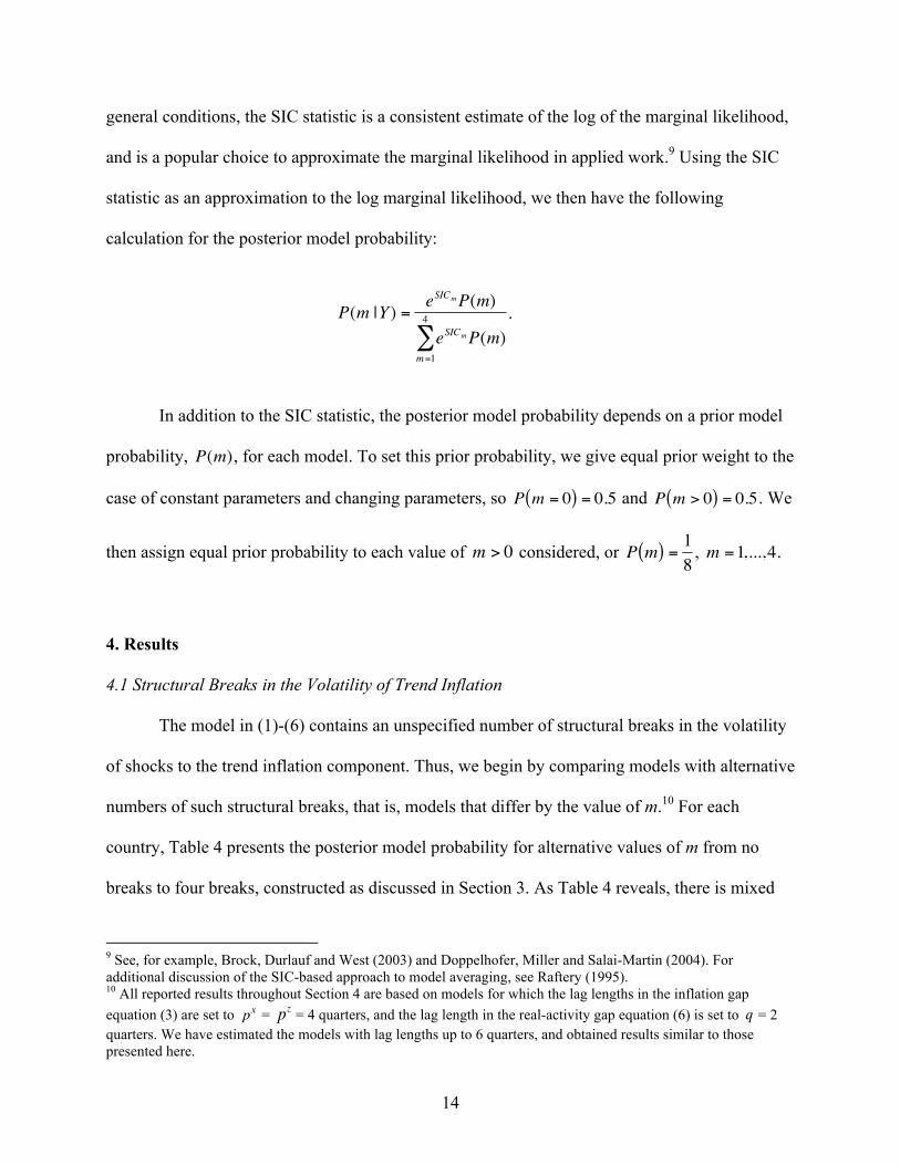
general conditions, the SIC statistic is a consistent estimate of the log of the marginal likelihood,

and is a popular choice to approximate the marginal likelihood in applied work.9 Using the SIC

statistic as an approximation to the log marginal likelihood, we then have the following

calculation for the posterior model probability:

€

P(m |Y ) =eSICmP(m)

eSICm

m=1

4

∑ P(m).

In addition to the SIC statistic, the posterior model probability depends on a prior model

probability,

€

P(m), for each model. To set this prior probability, we give equal prior weight to the

case of constant parameters and changing parameters, so

€

P m = 0( ) = 0.5 and

€

P m > 0( ) = 0.5. We

then assign equal prior probability to each value of

€

m > 0 considered, or

€

P m( ) =18

,

€

m =1,...,4.

4. Results

4.1 Structural Breaks in the Volatility of Trend Inflation

The model in (1)-(6) contains an unspecified number of structural breaks in the volatility

of shocks to the trend inflation component. Thus, we begin by comparing models with alternative

numbers of such structural breaks, that is, models that differ by the value of m.10 For each

country, Table 4 presents the posterior model probability for alternative values of m from no

breaks to four breaks, constructed as discussed in Section 3. As Table 4 reveals, there is mixed

9 See, for example, Brock, Durlauf and West (2003) and Doppelhofer, Miller and Salai-Martin (2004). For additional discussion of the SIC-based approach to model averaging, see Raftery (1995). 10 All reported results throughout Section 4 are based on models for which the lag lengths in the inflation gap equation (3) are set to

€

px =

€

pz = 4 quarters, and the lag length in the real-activity gap equation (6) is set to

€

q = 2 quarters. We have estimated the models with lag lengths up to 6 quarters, and obtained results similar to those presented here.

15

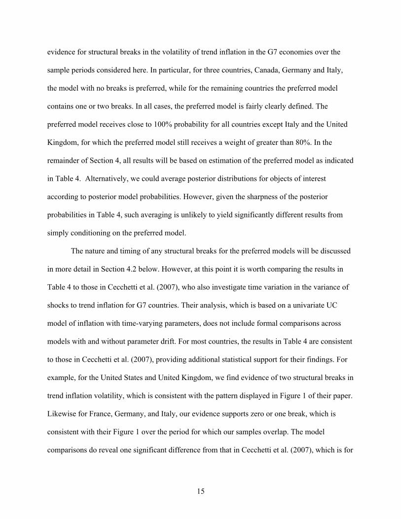
evidence for structural breaks in the volatility of trend inflation in the G7 economies over the

sample periods considered here. In particular, for three countries, Canada, Germany and Italy,

the model with no breaks is preferred, while for the remaining countries the preferred model

contains one or two breaks. In all cases, the preferred model is fairly clearly defined. The

preferred model receives close to 100% probability for all countries except Italy and the United

Kingdom, for which the preferred model still receives a weight of greater than 80%. In the

remainder of Section 4, all results will be based on estimation of the preferred model as indicated

in Table 4. Alternatively, we could average posterior distributions for objects of interest

according to posterior model probabilities. However, given the sharpness of the posterior

probabilities in Table 4, such averaging is unlikely to yield significantly different results from

simply conditioning on the preferred model.

The nature and timing of any structural breaks for the preferred models will be discussed

in more detail in Section 4.2 below. However, at this point it is worth comparing the results in

Table 4 to those in Cecchetti et al. (2007), who also investigate time variation in the variance of

shocks to trend inflation for G7 countries. Their analysis, which is based on a univariate UC

model of inflation with time-varying parameters, does not include formal comparisons across

models with and without parameter drift. For most countries, the results in Table 4 are consistent

to those in Cecchetti et al. (2007), providing additional statistical support for their findings. For

example, for the United States and United Kingdom, we find evidence of two structural breaks in

trend inflation volatility, which is consistent with the pattern displayed in Figure 1 of their paper.

Likewise for France, Germany, and Italy, our evidence supports zero or one break, which is

consistent with their Figure 1 over the period for which our samples overlap. The model

comparisons do reveal one significant difference from that in Cecchetti et al. (2007), which is for

16

the case of Canada. In particular, their Figure 1 suggests that Canadian trend inflation volatility

has followed a similar pattern to that in the U.S. and U.K., undergoing multiple structural breaks.

However, the model comparisons presented here suggest that the model with no breaks in trend

inflation volatility is strongly preferred to the model that includes breaks.

4.2 Estimates of Trend Inflation and Trend Inflation Volatility for the G7

In this section we present estimates of trend inflation,

€

π t , and estimates to the

(potentially) time varying variance of shocks to trend inflation,

€

σ v,t2 , using the preferred model as

identified in Table 4. Figure 1 displays the actual inflation rate along with the median of the

posterior distribution of

€

π t for each country. There are three similarities across countries in the

results of Figure 1 that we wish to highlight here. First, there is a general reduction in trend

inflation that begins in the late 1970s to early 1980s and continues to the end of the sample. For

most countries, trend inflation drifts downward over the past three decades, and is at its lowest

level toward the end of the sample period. The one exception to this is German trend inflation,

which displays a less obvious pattern of drift. Second, for the three countries for which the

sample period extends to the early 1960s, namely Canada, the United Kingdom, and the United

States, the estimates of

€

π t follow a “hump-shaped” pattern in which trend inflation is low in the

1960s, high in the 1970s, and trending downward beginning in the early 1980s. Third, for a

number of countries, most notably Canada, France, Italy and the United Kingdom, trend inflation

is on average above actual inflation for significant time periods in the 1980s and 1990s, which

means that the inflation gap was negative over these periods. This result is driven by substantial

deviations of unemployment above the estimated natural rate over these periods, and highlights

the role that the real-activity gap is playing in the identification of trend inflation for our model.

17

Indeed, such patterns are not a feature of the estimated trend inflation series for the G7 countries

obtained in the univariate analysis of Cecchetti et al. (2007).

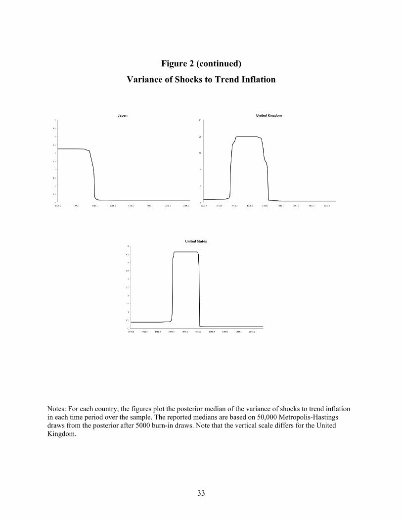
Figure 2 displays the posterior median of

€

σ v,t2 , the variance of shocks to trend inflation. It

is worth noting that when the preferred model includes structural breaks, the posterior

distribution of

€

σ v,t2 integrates out uncertainty regarding the location of these breaks, which

explains the smoother pattern to the posterior median of

€

σ v,t2 in some cases than would be

suggested by a structural break model with known break dates. The results in Figure 2 can

usefully be divided into two groups. First, for French, Japanese, U.K. and U.S. inflation, the

volatility of shocks to trend inflation display a pattern similar to that observed for the level of

trend inflation in Figure 1. In particular, when the level of trend inflation is high, the volatility of

trend inflation is also high. For these countries, the variance of shocks to trend inflation is at its

sample period low toward the end of the sample period, reaching levels corresponding to a

standard deviation of around 0.3 annualized percentage points for France, Japan and the United

States, and 0.6 annualized percentage points for the United Kingdom. Second, and as discussed

in Section 4.1 above, for Germany, Italy and Canada the preferred model includes no structural

breaks in the volatility of trend inflation. In these cases, the estimated full sample variance of

shocks to trend inflation is relatively low in all cases, and is comparable to the levels achieved

near the end of the sample by the other G7 countries.

It is worth noting that there are important examples of countries with similar estimated

patterns for the level of trend inflation that do not have similar estimated patterns for the

volatility of trend inflation, with Canada, the United States, and the United Kingdom providing a

leading example. Each of these countries have estimates of trend inflation that follow a hump-

shaped pattern over the sample. However, while the United States and United Kingdom show

18

strong evidence of a similar hump-shaped pattern for trend inflation volatility, there is very little

evidence of time variation in the volatility of trend inflation in Canada.

As we have discussed earlier, trend inflation is likely closely linked to long-horizon

inflation expectations, suggesting the results regarding trend inflation could alternatively be

interpreted as results regarding the role and evolution of long-horizon inflation expectations.

Thought of this way, the results suggest that long-horizon inflation expectations have played an

important role in the determination of actual inflation variability over the sample periods

considered here, and that long-horizon expectations of inflation are now “anchored” at low levels

in al G7 countries. Given the important role that the credibility of the monetary authority likely

has in the determination of long-horizon inflation expectations, it is notable that these similarities

exist despite the fact that there are substantial differences in the monetary institutions across

these countries, most notably the choice of whether or not to pursue an inflation targeting

framework.

4.3 Contribution of Inflation Components to Inflation Variation

We now turn to an investigation of the relative contribution of the various inflation

drivers in the model of (1)-(6) to realized inflation volatility. We begin by documenting the

relative contribution of the inflation trend and inflation gap for explaining realized variation in

total inflation. We then turn to the relative contribution of the real activity gap, supply shocks,

and the irregular component for explaining realized variation in the inflation gap.

To measure the relative importance of the inflation trend vs. the inflation gap for the

volatility of actual inflation, we construct counterfactual measures of inflation volatility. As the

model assumes that inflation contains a unit root, we focus on explaining the volatility of

19

changes to observed inflation at various horizons. Using the estimated model, we construct a

counterfactual series of inflation changes in which we set either changes to the inflation trend or

changes to the inflation gap equal to zero. We then compare the variation in this counterfactual

series with the variation in actual inflation changes. Formally, we construct counterfactual ratios

as follows:

€

R j =( ˜ π t − ˜ π t− j )

2

(π t −π t− j )2

t= j+1

T

∑ ,

where

€

˜ π t = π t for the inflation trend counterfactual ratio and

€

˜ π t = π tg for the inflation gap

counterfactual ratio. We construct

€

R j for each draw of

€

π t and

€

π tg taken from their respective

posterior distributions, which produces draws of

€

R j from its posterior distribution.

Table 5 presents the median and 10th and 90th percentiles of the posterior distribution for

the trend inflation counterfactual ratio at horizons of 1, 4, 12 and 24 quarters. It is important to

note that the trend inflation and inflation gap counterfactual ratios do not represent variance

decompositions because trend inflation and the inflation gap may not be independent of each

other. As a result, the trend inflation and inflation gap counterfactual ratios need not sum to

unity. However, for all the cases we consider here, the posterior median of the counterfactual

ratios do sum to roughly unity. Thus, for ease of presentation, we focus our attention on the trend

inflation counterfactual ratio in Table 5, with the understanding that the inflation gap

counterfactual is roughly one minus that for trend inflation.

There are three points from Table 5 that we wish to highlight here. First, there is a

general increase (decrease) across countries in the trend inflation (inflation gap) counterfactual

ratio as the horizon increases. This is not surprising as we would expect the inflation trend,

20

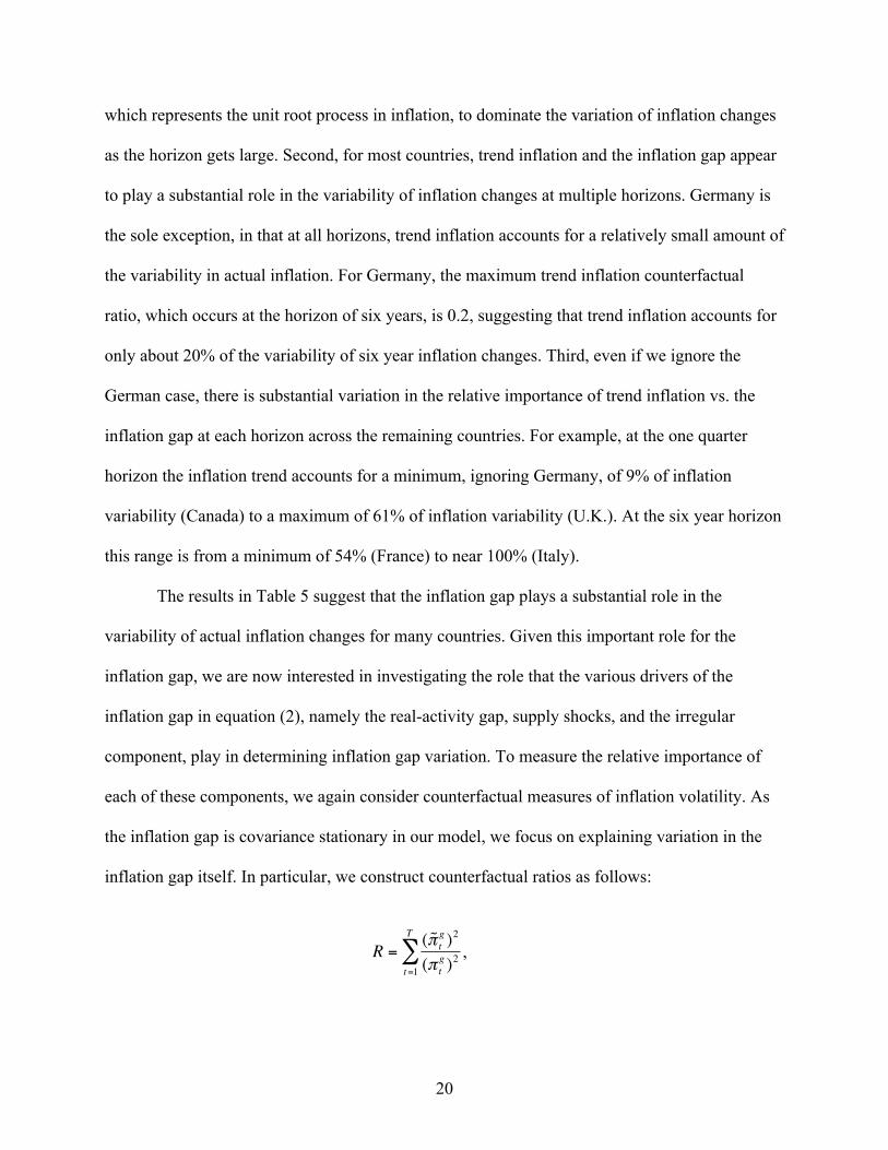
which represents the unit root process in inflation, to dominate the variation of inflation changes

as the horizon gets large. Second, for most countries, trend inflation and the inflation gap appear

to play a substantial role in the variability of inflation changes at multiple horizons. Germany is

the sole exception, in that at all horizons, trend inflation accounts for a relatively small amount of

the variability in actual inflation. For Germany, the maximum trend inflation counterfactual

ratio, which occurs at the horizon of six years, is 0.2, suggesting that trend inflation accounts for

only about 20% of the variability of six year inflation changes. Third, even if we ignore the

German case, there is substantial variation in the relative importance of trend inflation vs. the

inflation gap at each horizon across the remaining countries. For example, at the one quarter

horizon the inflation trend accounts for a minimum, ignoring Germany, of 9% of inflation

variability (Canada) to a maximum of 61% of inflation variability (U.K.). At the six year horizon

this range is from a minimum of 54% (France) to near 100% (Italy).

The results in Table 5 suggest that the inflation gap plays a substantial role in the

variability of actual inflation changes for many countries. Given this important role for the

inflation gap, we are now interested in investigating the role that the various drivers of the

inflation gap in equation (2), namely the real-activity gap, supply shocks, and the irregular

component, play in determining inflation gap variation. To measure the relative importance of

each of these components, we again consider counterfactual measures of inflation volatility. As

the inflation gap is covariance stationary in our model, we focus on explaining variation in the

inflation gap itself. In particular, we construct counterfactual ratios as follows:

€

R =( ˜ π t

g )2

(π tg )2

t=1

T

∑ ,

21

where

€

˜ π tg = δ j xt− j

j=0

px

∑ for the real-activity gap counterfactual ratio,

€

˜ π tg = γ j zt− j

j=0

pz

∑ for the supply

shock counterfactual ratio, and

€

˜ π tg =ω t for the irregular component counterfactual measure.

For each country, Table 6 presents the median and 10th and 90th percentiles of the

posterior distribution for each of these counterfactual ratios. We begin with the third column of

Table 6, which shows the counterfactual ratio for the irregular component. The posterior median

for this ratio ranges from a low of 0.09 in the United States to a high of 0.34 in Germany. As this

term represents the contribution of the error term in the inflation gap equation (3), this suggests

that the real-activity gap and supply shock terms explain a substantial portion of inflation gap

variability for all countries.

Turning to the contribution of the real-activity gap and supply shocks, the first column of

Table 6 presents the real-activity gap counterfactual ratios, and demonstrates a striking

difference in the role played by the real activity gap for explaining variation in the inflation gap.

For some countries, notably Japan and the United States, the counterfactual ratio for the real

activity gap is quite small, accounting for less than 10% of inflation gap variability. For other

countries, notably Canada and the United Kingdom, the inflation gap accounts for greater than

50% of inflation gap variability. Finally, for the remaining countries, France, Germany and Italy,

the real-activity gap counterfactual ratio is in the range of 0.3-0.4. Given the differences across

countries in the real-activity gap counterfactuals, it is not surprising that we observe

corresponding differences in the supply shock counterfactual ratio, presented in the second

column of Table 6. In particular, for the U.S. and Japan, the supply shock counterfactual is quite

high, over 0.7 in both cases, while for the United Kingdom the ratio is below 0.10.

Taken together, these results suggest that the inflation gap has contributed significantly to

the variability of changes to realized inflation in all of the G7 countries, and that the real-activity

22

gap appears to be a significant driver of the inflation gap for a number of the G7 countries. We

interpret this as an empirical success for the NKPC, once augmented to include a trend inflation

component, in these countries. Interestingly however, this is not the case for the United States

and Japan, for which the real-activity gap explains only a small portion of the variability in the

inflation gap. The results for the United States are particularly interesting as several recent

studies, such as Cogley and Sbordone (2008), find that the fit of the NKPC for U.S. inflation is

improved once the model is augmented with a trend inflation component. Our results suggest

that despite this improvement, the role played by the real-activity gap for explaining short-run

variation in U.S. inflation is minor.

5. Conclusion

We have estimated a bivariate unobserved components model of inflation and

unemployment in the G7 countries using Bayesian techniques, and used it to shed light on the

relative importance of trend inflation, the real-activity gap, and supply shocks for explaining

variability in realized inflation. Our results reveal that both trend inflation and the deviation of

inflation from trend inflation, or the so-called inflation gap, have contributed significantly to

actual variation in inflation changes at horizons of one quarter to six years in most countries.

Further, we find that the real activity gap is an important determinant of the inflation gap for

several countries, which we interpret as an empirical success for the New Keynesian Phillips

Curve augmented to include a role for trend inflation. Notably however, the United States is not

one of these countries.

We also have provided new estimates of trend inflation in the G7 countries that take into

account information in the real-activity gap for identification, as well as formal comparisons of

23

models with and without time-variation in the volatility of shocks to trend inflation. These

comparisons reveal important changes in the volatility of trend inflation in some countries but

not others. Both the level and volatility of trend inflation is quite low in all countries near the end

of the sample period, which is suggestive that long-horizon inflation expectations are anchored at

low levels across the G7 economies.

A primary focus of our analysis has been on explaining the determinants of the inflation

gap. However, for many countries, trend inflation has also been an important contributor to the

variability of observed inflation. This result suggests that it is important to understand the

determination of trend inflation in order to adequately explain the historical path of actual

inflation in most countries. Given the link between trend inflation and long-horizon inflation

expectations, one approach to understand the evolution of trend inflation is to understand the

determinants of long-horizon inflation expectations. To this end, a number of recent studies,

including Clark and Davig (2008) and Kiley (2008) for U.S. inflation and Barnett, Groen and

Mumtaz (2009) for U.K. inflation have investigated the effects of various types of shocks on

long-horizon inflation expectations. Further research on this topic is likely to be an important

avenue for improved understanding of the inflation process in the G7.

24

References

Barnett, A., Groen, J.J.J. and H. Mumtaz, 2009, Time-Varying Inflation Expectations and Economic Fluctuations in the United Kingdom: A Structural VAR Analysis, mimeo.

Bernanke, B., July 2007, Inflation Expectations and Inflation Forecasting, Speech presented at

the Monetary Economics Workshop of the National Bureau of Economic Research Summer Institute, Cambridge, MA.

Beveridge, S. and C.R. Nelson, 1981, A New Approach to Decomposition of Economic Time

Series into Permanent and Transitory Components with Particular Attention to Measurement of the Business Cycle, Journal of Monetary Economics 7, 151-174.

Brock, W.A., S.N. Durlauf, and K. D. West, 2003, Policy evaluation in uncertain economic

environments, Brookings Papers on Economic Activity 1, 235-301. Bryan, M.F. and S.G. Cecchetti, 1994, Measuring Core Inflation, in N.G. Mankiw (ed.),

Monetary Policy, Chicago University Press, Chicago, IL. Carter, C.K. and R. Kohn, 1994, On Gibbs Sampling for State Space Models, Biometrika 81,

541-553. Cecchetti, S.G., Hooper, P., Kasman, B.C., Schoenholtz, K.L. and M.W. Watson., 2007,

Understanding the Evolving Inflation Process, in U.S. Monetary Policy Forum Report No. 1, Rosenberg Institute for Global Finance, Brandeis International Business School and Initiative on Global Financial Markets, University of Chicago Graduate School of Business.

Clark, T.E. and T. Davig, 2008, An Empirical Assessment of the Relationships Among Inflation

and Short- and Long-Term Expectations, Federal Reserve Bank of Kansas City Research Working Paper No. 08-05.

Cogley, T., Primiceri, G.E., and T.J. Sargent, 2010, Inflation-Gap Persistence in the U.S.,

American Economic Journal: Macroeconomics 2, 43-69. Cogley, T. and A.M. Sbordone, 2008, Trend Inflation, Indexation, and Inflation Persistence in

the New Keynesian Phillips curve, American Economic Review 98, 2101-2126. Doppelhofer, G., R. Miller, and X. Sala-i-Martin, 2004, Determinants of long-term growth: A

Bayesian averaging of classical estimates (BACE) approach, American Economic Review 94, 813-835.

Estrella, A., and J.C. Fuhrer, 2002, Dynamic Inconsistencies: Counterfactual Implications of a

Class of Rational-Expectation Models, American Economic Review 92, 1013-1028.

25

Fuhrer, J.C., 1997, The (Un)Importance Of Forward Looking Behavior In Price Specifications,

Journal of Money, Credit and Banking 29, 338-350. Fuhrer, J.C. and G. Moore, 1995, Inflation Persistence, The Quarterly Journal of Economics 110,

127-159. Gali, J. and M. Gertler, 1999, Inflation Dynamics: A Structural Econometric Analysis, Journal

of Monetary Economics 44, 195-222. Gali, J., Gertler, M. and D. Lopez-Salido, 2001, European Inflation Dynamics, European

Economic Review 45, 1237-1270. Goodfriend, M. and R.G. King, 2009, The Great Inflation Drift, NBER Working Paper No.

14862. Gordon, R. J., 1982, “Inflation, Flexible Exchange Rates and the Natural Rate of

Unemployment,” in Baily, M.N., ed., Workers, Jobs and Inflation, Washington, DC: Brookings Institution, pp. 88-152.

Gordon, R. J., 1997, “The Time-Varying NAIRU and its Implications for Economic Policy,”

Journal of Economic Perspectives 11, 11-32. Gordon, R. J., 1998, “Foundations of the Goldilocks Economy: Supply Shocks and the Time

Varying NAIRU,” Brookings Papers on Economic Activity 2, 297-333. Harvey, A.C., 2008, Modeling the Phillips Curve with Unobserved Components, Cambridge

Working Papers in Economics No. 0805. Kang, K.H., Kim, C.-J. and J. Morley, 2010, Changes in U.S. Inflation Persistence, Studies in

Nonlinear Dynamics & Econometrics 13. Kiley, M.T., 2008, Monetary Policy Actions And Long-Run Inflation Expectations, Federal

Reserve Finance and Economics Discussion Series working paper no. 2008-03. Koop, G., 2003, Bayesian Econometrics, John Wiley and Sons, New York, NY. Laubach, T., 2001, Measuring the NAIRU: Evidence from Seven Economies, The Review of

Economics and Statistics 83, 218-231. Lee, J. and C.R. Nelson, 2007, Expectation Horizon and the Phillips Curve: The Solution to an

Empirical Puzzle, Journal of Applied Econometrics 22, 161-178. Manopimoke, P., 2010, Trend Inflation and the New Keynesian Phillips Curve, mimeo.

26

Piger, J. and R. H. Rasche, 2008, Inflation: Do Expectations Trump the Gap?, International

Journal of Central Banking 4, 85-116. Raftery, A., 1995, Bayesian Model Selection in Social Research, Sociological Methodology 25,

111-163. Roberts J., 2001, How Well Does the New Keynesian Sticky-Price Model Fit the Data?, Federal

Reserve Finance and Economics Discussion Series working paper no. 2001-13. Rudd, J. and K. Whelan, 2005, Does Labor’s Share Drive Inflation?, Journal of Money, Credit

and Banking 37, 297-312. Staiger, D., Stock, J. and M.W. Watson, 1997, How Precise are Estimates of the Natural Rae of

Unemployment, in C. Romer and D. Romer (eds.), Reducing Inflation: Motivation and Strategy, Chicago University Press, Chicago, IL.

Stock, J. H. and M.W. Watson, 2007, “Why has U.S. Inflation Become Harder to Forecast?,”

Journal of Money, Credit and Banking 39, 3-33. Wang, J. and E. Zivot, 2000, A Bayesian Time Series Model of Multiple Structural Changes in

Level, Trend, and Variance, Journal of Business and Economic Statistics 18, 374-86.

27

Table 1 Sample Periods Data Sample Canada 1961:Q2 - 2006:Q2 France 1978:Q2 - 2006:Q2 Germany 1978:Q2 - 2006:Q2 Italy 1982:Q2 - 2006:Q2 Japan 1970:Q2 - 2006:Q2 United Kingdom 1963:Q2 - 2006:Q2 United States 1957:Q2 - 2007:Q2 Table 2 Dummy Variable Dates Date Event

1991:1 Cigarette Tax Change Canada

1994:1 – 1994:2 Cigarette Tax Change

1991:1-1991:4 Reunification Germany

1993:1 VAT Introduction

Japan 1997:2 Consumption Tax Increase

United Kingdom 1990:2 Poll Tax Introduction

28

Table 3 Augmented Dickey Fuller Tests Unemployment

Rate Total CPI Inflation

Food and Energy CPI Inflation

Canada 0.33 0.27 0.00 France 0.10 0.47 0.00 Germany 0.06 0.13 0.01 Italy 0.72 0.01 0.00 Japan 0.53 0.10 0.00 United Kingdom 0.13 0.04 0.01 United States 0.01 0.08 0.00 Notes: Table contains the MacKinnon (1996) p-values for the Augmented Dickey Fuller test for a unit root in the indicated series. Lag lengths were selected using the Akaike Information Criteria based on a maximum lag length of 4 quarterly lags. Table 4 Posterior Probability for Number of Breaks in Trend Inflation Volatility

Number of Breaks 0 1 2 3 4 Canada 97.6% 2.4% 0.0% 0.0% 0.0% France 0.0% 99.9% 0.1% 0.0% 0.0% Germany 99.8% 0.2% 0.0% 0.0% 0.0% Italy 87.8% 11.6% 0.6% 0.0% 0.0% Japan 0.0% 99.9% 0.1% 0.0% 0.0% United Kingdom 0.0% 0.1% 82.1% 17.1% 0.7% United States 0.0% 0.0% 100.0% 0.0% 0.0% Notes: For each country, the table contains the posterior probability of alternative numbers of structural breaks in the variance of shocks to trend inflation. Posterior probabilities are based on the asymptotic approximation given by the SIC, as discussed in Section 3.

29

Table 5 Contribution of Changes in Trend Inflation to Variability of Changes in Inflation Horizon (Quarters) 1 4 12 24 Canada 0.06 0.09 0.13 0.15 0.21 0.28 0.27 0.37 0.47 0.48 0.65 0.87 France 0.26 0.34 0.43 0.40 0.49 0.58 0.38 0.51 0.65 0.38 0.54 0.71 Germany 0.03 0.06 0.09 0.09 0.14 0.22 0.11 0.18 0.30 0.10 0.20 0.35 Italy 0.27 0.41 0.59 0.34 0.47 0.62 0.42 0.56 0.73 0.73 1.01 1.35 Japan 0.14 0.18 0.23 0.33 0.40 0.46 0.37 0.44 0.52 0.53 0.68 0.78 United Kingdom 0.49 0.61 0.72 0.56 0.67 0.78 0.59 0.70 0.82 0.69 0.78 0.90 United States 0.37 0.43 0.49 0.49 0.56 0.64 0.50 0.57 0.67 0.66 0.73 0.80 Notes: For each country, the table gives the counterfactual ratio of the variability of changes in trend inflation at alternative horizons to the variability of changes in actual inflation at the same horizon. The median of the posterior distribution of the counterfactual ratio is given in bold, along with the 10th and 90th percentiles of the posterior distribution. Reported statistics are based on 50,000 Metropolis-Hastings draws from the posterior after 5000 burn-in draws. Table 6 Contribution of Inflation Gap Components to Variability of Inflation Gap Real Activity Gap Supply Shocks Irregular Component Canada 0.34 0.53 0.72 0.17 0.29 0.44 0.11 0.18 0.26 France 0.15 0.42 0.68 0.18 0.34 0.59 0.10 0.18 0.31 Germany 0.14 0.32 0.56 0.25 0.42 0.62 0.24 0.34 0.46 Italy 0.12 0.37 0.75 0.14 0.37 0.70 0.12 0.28 0.55 Japan 0.01 0.04 0.22 0.56 0.73 0.86 0.15 0.20 0.27 United Kingdom 0.47 0.76 0.94 0.01 0.05 0.15 0.13 0.32 0.72 United States 0.04 0.10 0.22 0.59 0.73 0.85 0.06 0.09 0.12 Notes: For each country, the table gives the counterfactual ratio of the variability of the determinants of the inflation gap from equation (3) to the variability of the actual inflation gap at the same horizon. The median of the posterior distribution of each counterfactual ratio is given in bold, along with the 10th and 90th percentiles of the posterior distribution. Reported statistics are based on 50,000 Metropolis-Hastings draws from the posterior after 5000 burn-in draws.

30

Figure 1

Actual Inflation and Estimated Trend Inflation

31

Figure 1 (continued)

Actual Inflation and Estimated Trend Inflation

Notes: For each country, the figures plot the actual quarterly inflation rate (red line), measured using the CPI, along with the median of the posterior distribution for trend inflation (black line). The reported medians are based on 50,000 Metropolis-Hastings draws from the posterior after 5000 burn-in draws. Note that the vertical scale differs across countries.

32

Figure 2

Variance of Shocks to Trend Inflation

33

Figure 2 (continued)

Variance of Shocks to Trend Inflation

Notes: For each country, the figures plot the posterior median of the variance of shocks to trend inflation in each time period over the sample. The reported medians are based on 50,000 Metropolis-Hastings draws from the posterior after 5000 burn-in draws. Note that the vertical scale differs for the United Kingdom.