Inflation and Uncertainty at Short and Long Horizons · PDF fileInfation and Uncertainty at...
40
LAURENCE BALL Princeton University STEPHEN G. CECCHETTI Ohio State University Infation and Uncertainty at Short and Long Horizons ALTHOUGH MOST ECONOMISTS agree that inflationis costly, there is no consensusabout why. Many traditionally citedcosts, suchas deadweight loss from the inflation"tax," seem too small to justify concern about moderate inflation. One approach is to arguethat inflation of 10percent or 15 percent would not be particularly costly if it were constant and fully anticipated, but thata rise in the level of inflation raises uncertainty aboutfutureinflation. In the absence of perfect indexation,such uncer- tainty has significant costs, including arbitrary redistributions, relative price variation, and fewer long-term contracts, such as loans to finance investment. I This view implies that understanding the costs of inflation requires that we understand the connection between the level of inflationand uncertainty. The idea that high inflation leads to greateruncertainty is suggested in ArthurOkun's "The Mirageof Steady Inflation"and in Milton Friedman'sNobel lecture, and many economists treat it as a stylizedfact.2But empirical studies of the inflation-uncertainty relation report conflicting results, and the issue appears unsettled. We are grateful for suggestionsfrom RobertBarsky, Alan Blinder,John Campbell, AlexCukierman, Martin Evans, Paul Evans, N. Gregory Mankiw, Jeffrey Miron, Whitney Newey, Pierre Perron, Richard Startz, Paul Wachtel,members of the Brookings Panel, and seminarparticipants at Princeton University. Cecchetti acknowledges financial support from the National Science Foundation. 1. Fordiscussions of the costs of inflation uncertainty, see JaffeeandKleiman (1977) andFischer andModigliani (1978). 2. Okun (1971); M. Friedman (1977). 215
Transcript of Inflation and Uncertainty at Short and Long Horizons · PDF fileInfation and Uncertainty at...

LAURENCE BALL Princeton University
STEPHEN G. CECCHETTI Ohio State University
Infation and Uncertainty at Short and Long Horizons
ALTHOUGH MOST ECONOMISTS agree that inflation is costly, there is no consensus about why. Many traditionally cited costs, such as deadweight loss from the inflation "tax," seem too small to justify concern about moderate inflation. One approach is to argue that inflation of 10 percent or 15 percent would not be particularly costly if it were constant and fully anticipated, but that a rise in the level of inflation raises uncertainty about future inflation. In the absence of perfect indexation, such uncer- tainty has significant costs, including arbitrary redistributions, relative price variation, and fewer long-term contracts, such as loans to finance investment. I
This view implies that understanding the costs of inflation requires that we understand the connection between the level of inflation and uncertainty. The idea that high inflation leads to greater uncertainty is suggested in Arthur Okun's "The Mirage of Steady Inflation" and in Milton Friedman's Nobel lecture, and many economists treat it as a stylized fact.2 But empirical studies of the inflation-uncertainty relation report conflicting results, and the issue appears unsettled.
We are grateful for suggestions from Robert Barsky, Alan Blinder, John Campbell, Alex Cukierman, Martin Evans, Paul Evans, N. Gregory Mankiw, Jeffrey Miron, Whitney Newey, Pierre Perron, Richard Startz, Paul Wachtel, members of the Brookings Panel, and seminar participants at Princeton University. Cecchetti acknowledges financial support from the National Science Foundation.
1. For discussions of the costs of inflation uncertainty, see Jaffee and Kleiman (1977) and Fischer and Modigliani (1978).
2. Okun (1971); M. Friedman (1977).
215

216 Brookings Papers on Economic Activity, 1:1990
To try to resolve the empirical stand-off, we focus on the distinction between short-term and long-term uncertainty-that is, uncertainty over different horizons. The experience of many countries fits a simple statistical model in which there are both permanent and temporary shocks to inflation. Permanent shocks are shifts in trend inflation, and temporary shocks are fluctuations around the trend. Uncertainty about next quarter's inflation depends mainly on the variance of temporary shocks, while uncertainty about inflation over several years depends mainly on the variance of permanent shocks. Our central finding is that the level of inflation has a much stronger effect on the variance of permanent shocks than on the variance of temporary shocks, and thus a stronger effect on uncertainty at long horizons.
This finding has several important implications. First, it helps to reconcile the divergent results of previous studies. Whether analysts find an inflation-uncertainty link depends largely on the horizons they consider. Second, the finding helps distinguish between alternative explanations for the inflation-uncertainty relation. Because permanent changes in inflation involve changes in monetary policy, the finding supports the arguments of Okun, Friedman, and others that high inflation makes policy less stable. Third, the finding sharpens our understanding of the costs of inflation. Most of the costs of uncertainty about inflation, such as added risk in long-term contracts, involve uncertainty over several years or more. Thus our conclusion that high inflation raises long-term uncertainty strengthens the case for policymakers to keep inflation low.
We have several related findings. The first concerns the distinction between inflation variability and inflation uncertainty-between the variance of changes in inflation and the variance of unanticipated changes. We find no evidence for Stanley Fischer's suggestion that high inflation raises variability but not uncertainty; instead, it raises both.3 Second, the inflation-uncertainty relation across countries differs from the relation over time in a given country. Across countries, short-term as well as long-term uncertainty rises with average inflation. Finally, the inflation-uncertainty relation in countries with very high inflation is similar to the relation in moderate-inflation countries, though somewhat stronger.
3. Fischer(1981).

Laurence Ball and Stephen G. Cecchetti 217
Explanations for the Inflation-Uncertainty Relation
To review alternative explanations for a relation between inflation and uncertainty, we focus on the following question. Consider two moderate- inflation economies-either different countries or the same country during different periods-with different trend rates of inflation, one high and one low. Is uncertainty about inflation-the variance of errors in optimal forecasts-higher in the economy with the higher trend?
We assume that trend inflation is determined by trend money growth, and that inflation varies around its trend because of monetary and other demand and supply shocks. In this framework, there are two reasons for inflation uncertainty to be high when the trend is high. First, inflation might vary more around its trend when the trend is high. Second, a high trend might imply that the trend itself is less stable. These explanations have different implications for the horizon over which inflation raises uncertainty. We discuss the two explanations in turn.
Why might inflation vary more around its trend when the trend is high? The answer is not obvious, but several authors present models with this property. In some models, an exogenous rise in trend inflation causes greater variability. Joel Hasbrouck, for example, argues that individuals adjust their cash balances more frequently at high inflation. The implication is that money demand responds more quickly to shocks, which causes inflation to vary more. Ball, Gregory Mankiw, and David Romer argue that high trend inflation reduces nominal price rigidity and thus steepens the short-run Phillips curve. As a result, shocks to aggregate demand have smaller effects on output but larger effects on inflation.4
Alex Cukierman and Allan Meltzer, as well as Michael Devereux, derive links between trend inflation and fluctuations around the trend when the trend is endogenous. They use the Barro-Gordon model of "time-consistent" policy, in which the output effects of monetary surprises tempt the Federal Reserve into creating positive trend inflation. In both papers, a change that raises inflation uncertainty also increases the effects of surprises, which leads to a higher trend. In Cukierman and Meltzer's paper, the change is an increase in monetary control errors,
4. Hasbrouck (1979); Ball, Mankiw, and Romer (1988).

218 Brookings Papers on Economic Activity, 1:1990
which slows the public's revision of expectations after a surprise. In Devereux's paper, the change is an increase in the variance of real shocks, which raises the effects of surprises by decreasing wage index- ation.'
While these models may have elements of truth, they cannot fully capture the sources of inflation uncertainty. In the models, inflation is uncertain because shocks or control errors cause it to fluctuate around its trend. In actual economies, inflation is also uncertain because the trend itself may change. Because trend inflation is determined by trend money growth, shifts in the trend involve a shift in the policy of the Federal Reserve. The Federal Reserve may reduce trend money growth to disinflate, or it may allow the trend to rise to accommodate fiscal policy or a supply shock.
These possibilities are explored in the second set of theories about the inflation-uncertainty link-theories in which shifts in trend inflation are more likely when the trend is high. Drawing on arguments by Dennis Logue and Thomas Willett, Milton Friedman, and others, Ball presents a model in which trend inflation is less stable when it is high.6 The intuitive idea is simple. In a period of low inflation, such as the early 1960s in the United States, the consensus is that policymakers will try to keep inflation low. Inflation may arise at some point because the Federal Reserve accommodates a shock, but it is unlikely that the Federal Reserve will simply decide to raise inflation. In contrast, when trend inflation is high it is not clear what the Federal Reserve will do, because it faces a dilemma: it would like to disinflate, but fears the recession that would probably result. It is likely that disinflation will occur eventually, but the timing is uncertain. For example, in the late 1970s, it would have been difficult to predict the exact onset of the sharp disinflation of 1981-82. Ball formalizes this idea by assuming that policymakers differ in their views of the relative costs of unemployment and inflation and thus of the desirability of disinflation. When inflation is high, the public is uncertain about future inflation because it does not know which views will prevail.
In Ball's model, high inflation creates uncertainty about disinflation- about whether trend inflation will fall. High trend inflation might also
5. Cukierman and Meltzer (1986); Devereux (1989); Barro and Gordon (1983). 6. Logue and Willett (1976); M. Friedman (1977); Ball (1990).

Laurence Ball and Stephen G. Cecchetti 219
raise uncertainty by causing the public to fear that the trend will rise further. In "The Mirage of Steady Inflation," Okun describes what happens if policymakers accept high inflation to accommodate a shock: "Would not such a shift in policy have to be read as indicative of future action? Can a government that shifts its inflation tolerance level from 2 to 5 percent convince anyone that it will vigorously combat 8 percent inflation in the event of unforeseen excess demand or another unfavor- able surprise in the Phillips curve? . .. [A] decision to live with inflation would trigger off expectations of larger and more variable rates of price increase."7 In other words, by accommodating an inflationary shock, the Federal Reserve signals a willingness to accommodate future shocks; the unpredictability of future shocks creates uncertainty about future inflation. In contrast, a nonaccommodative policy makes it clear that the Federal Reserve is committed to keeping inflation under control. Paul Volcker's tough policy in the early eighties made the public more confident that inflation would stay low in the mid-eighties.
These two sets of theories have different implications for the horizon over which inflation raises uncertainty. If high inflation implies greater fluctuations around trend but does not affect the trend itself, then it may greatly increase uncertainty about next quarter's inflation, but have little effect on long-run uncertainty. In contrast, if high inflation implies a less stable trend, then it raises long-run uncertainty. It has little effect on short-run uncertainty assuming the latter is dominated by fluctuations around trend. Our statistical model formalizes these ideas.8
Previous Evidence and a First Look at U.S. Data
The initial empirical evidence of a link between the level and variability of inflation is contained in cross-country studies by Okun, Logue and Willett, Edward Foster, and others in the 1970s.9 For a given country, these authors compute the sample mean of annual postwar inflation and a measure of variability-either the sample variance or the average squared change in inflation. They find a strong positive cross-country
7. Okun (1971, p. 490). 8. The distinction between long-run and short-run inflation uncertainty is discussed
by Klein (1976) and by Fischer (1981). Fischer suggests that high inflation raises long-run uncertainty by increasing the likelihood of a shift in monetary policy.
9. Okun (1971); Logue and Willett (1976); Foster (1978).

220 Brookings Papers on Economic Activity, 1:1990
correlation between the mean and the measure of variability-in other words, that countries with high inflation rates also have more variable inflation. Some studies report a nonlinear relation, one that is stronger across high- and moderate-inflation countries than across moderate- inflation countries only. But usually the studies find a significant relation over all ranges of inflation.
Papers by Fischer and John Taylor show that the positive correlation between means and variances holds across time as well as across countries.10 Fischer splits postwar U.S. data into three- and five-year subperiods and finds a positive correlation across periods. Taylor uses ten-year subperiods for seven OECD countries and achieves similar results.
Unfortunately for lovers of tidy stylized facts, the most prominent inflation-uncertainty study of the 1980s-Robert Engle's 1983 paper- reaches a different conclusion. Engle estimates a forecasting equation for quarterly inflation in the postwar United States. He then uses his ARCH technique to construct a time series for the variance of unantici- pated shocks to inflation, with the variance in a given quarter measuring uncertainty about inflation in the next quarter. Engle finds that the variance is uncorrelated with the current level of inflation-that high inflation in one quarter does not lead to greater uncertainty about inflation in the next quarter. In particular, his variance estimates are roughly the same in the low-inflation 1960s as in the high-inflation 1970s. Subsequent estimates of ARCH models confirm these findings. "I
In trying to reconcile Engle's findings with other studies, Fischer suggests that high inflation raises inflation variability but not inflation uncertainty. That is, when inflation is high it varies considerably, but the movements are largely forecastable, so unanticipated changes in inflation are not especially large. An obvious and simpler interpretation, however, is that Engle's results differ from earlier ones because he considers a much shorter horizon. Perhaps current inflation has little effect on variability (or uncertainty) over the next quarter, but a signifi- cant effect on variability over the next five years. Such a finding could explain the results of pre-Engle studies, which usually measure variabil- ity over several years.
10. Fischer(1981);Taylor(1981). 11. Cosimano and Jansen (1988).

Laurence Ball and Stephen G. Cecchetti 221
Taylor's study provides a piece of evidence that horizons are impor- tant. For each of seven countries, Taylor estimates a forecasting equation for inflation and computes the variance of unanticipated inflation. He finds that the cross-country relation between mean inflation and this variance is positive and similar to the relation between the mean and the ordinary sample variance. The finding suggests that Fischer's distinction between variability and uncertainty is not important. One explanation for the difference between Engle's and Taylor's results is that, although both consider uncertainty about the next period, Engle uses quarterly data and Taylor uses annual data and thus considers uncertainty over a longer horizon. (Of course other differences might explain the results; for example, Engle studies a time series and Taylor a cross-section.)
Another relevant strand of research is the work of Benjamin Klein and of Robert Barsky on the persistence of U.S. inflation.12 As trend inflation has risen over the past 100 years, the persistence of changes in inflation has also increased. Barsky, for example, finds that quarterly inflation was roughly white noise during 1870-1913, followed auto- regressive processes during 1919-38 and 1947-59, and has followed a nonstationary process-so that changes in inflation are largely perma- nent-since 1960. As explained below, for a given variance of innovations in inflation, greater persistence implies greater uncertainty over long but not short horizons. Thus Klein's and Barsky's results support our hypothesis that a rise in inflation affects long-run uncertainty.
To motivate our own statistical model, we perform a preliminary analysis of U.S. data for 1954-89. We compute simple measures of the inflation level-variability relation and ask whether results are sensitive to horizons. Table 1 reports the results of splitting quarterly inflation data into nonoverlapping periods and computing the correlation of sample means and variances across periods. We use seasonally adjusted data on both the implicit GNP deflator and the CPI-U.13 The mean- variance correlation increases strongly with the lengths of periods. For the deflator, the correlation is 0.18 for one-year periods. It rises to 0.43 forfour-year periods and 0.94 for ten-year periods. The pattern is similar for the CPI, although the correlations are somewhat larger for short
12. Klein (1976); Barsky (1987). 13. The data are taken from Citibase. For the CPI-U, inflation is the percentage change
in the index from the last month of the previous quarter to the last month of the current quarter. We use the CPI-U for all iterris.

222 Brookings Papers on Economic Activity, 1:1990
Table 1. Subperiod Correlations of Mean and Variance of Inflation, United States, 1954-89a
Correlation
Length of Consumer subperiods GNP price
in years deflator indexb
1 0.180 0.318 2 0.309 0.670 3 0.360 0.629 4 0.433 0.902 5 0.772 0.768 6 0.933 0.848 7 0.459 0.987 8 0.825 0.859 9 0.788 0.969
10 0.942 0.966
Source: Citibase. Quarterly data, seasonally adjusted, for implicit GNP deflator and CPI-U for all items. a. Subperiods are nonoverlapping intervals of indicated length. b. For the CPI-U, inflation is the percentage change in the index from the last month of the previous quarter to
the last month of the current quarter.
periods.(While suggestive, the results for 10-year periods are imprecise because there are only three nonoverlapping observations.)
Table 2 reports another simple measure of the relation between the level of inflation and variability: the correlations between current infla- tion, ur,, and the squared change in inflation over x quarters for various values of x, (',r,+ - Tr,)2. Figure 1 plots the correlations against x. For the GNP deflator, the correlation when x = 1 is 0.09-there is almost no relation between the level and variability over the next quarter. The correlation rises as x rises, reaching 0.19-0.42 for x = 4 to x = 20 (roughly one to five years ahead). At even longer horizons, the correlation drops; it is near zero by x = 40. The CPI results are similar: the correlation is 0.21 for x = 1 and rises to a peak of 0.60 for x = 18.
What explains the hump-shaped pattern of correlations? The increase as x rises from 1 to 20 suggests that the level of inflation has a stronger effect on variability over several years than over the next quarter, as predicted by some of the theories described above. The weak correlation at very long horizons suggests that current inflation is uninformative about inflation in the distant future. Variability between 1990 and 2000 depends largely on the level of inflation in the late 1990s, which is difficult to predict based on the 1990 level. (Results for long horizons should

Laurence Ball and Stephen G. Cecchetti 223
Table 2. Correlations of Level and Squared Change in Inflation over Various Horizons, United States, 1954-89
Length of Correlation
horizon in GNP quarters (x) deflator CPIa
1 0.086 0.213 2 0.134 0.395 3 0.121 0.333 4 0.192 0.376 5 0.357 0.412 6 0.313 0.405 7 0.304 0.439 8 0.344 0.447 9 0.207 0.410
10 0.303 0.422 12 0.366 0.470 14 0.416 0.530 16 0.282 0.491 18 0.323 0.602 20 0.355 0.572 24 0.211 0.514 28 0.133 0.396 32 0.197 0.383 36 0.201 0.279 40 0.055 0.162 44 - 0.005 0.127 48 -0.071 0.153 50 - 0.045 0.016
Source: Same as table 1. The correlations are between rr1 and (rrt+, - rrt)2 for various horizons, x. a. See note b, table 1.
again be interpreted cautiously because we have few nonoverlapping observations.)
Comparing data at different frequencies also illuminates the role of forecast horizons. For annual deflator data, the correlation between inflation and its squared change is 0.22 for x = 1, compared with 0.09 for quarterly data. For the CPI, the correlation for x = 1 is 0.48 for annual data, 0.21 for quarterly data, and 0.10 for monthly data. The level- variability correlation increases monotonically with the length of a period. These results increase our suspicion that the differences between Engle's and Taylor's results are explained by differences between quarterly and annual data.

224 Brookings Papers on Economic Activity, 1:1990
Figure 1. Correlations of Level and Squared Change in Inflation, Consumer Price Index and GNP Deflator, United States, 1954-89
Correlation
0.6-
0.2
0.0 I (ille>orS
0 5 10 15 20 25 30 35 40 45 50 Length of horizon in quarters
Source: Citibase. Quarterly data, seasonally adjusted, for implicit GNP deflator and CPI-U for all items. The correlations are of nt1 and (rrT+t - qrt)2 for various horizons, x.
a. See note b, table 1.
A Statistical Model of Inflation
This section presents our basic statistical model and then shows how the model captures the inflation-uncertainty relation at various horizons.
Basic Model
Engle's approach to the inflation-uncertainty link is to estimate a forecasting equation for inflation and look for a relation between current inflation and the variance of innovations. Unfortunately, such an ap- proach does not allow us to address our question. In such a framework,

Laurence Ball and Stephen G. Cecchetti 225
uncertainty at any horizon is proportional to the variance of the inno- vation. (If, for example, inflation is a random walk, then the x-period- ahead forecast variance equals x times the variance of the innovation.) To the extent that the level of inflation affects the variance of innovations, it has the same proportional effect on uncertainty at all horizons.
To allow different inflation-uncertainty relations at different horizons, we consider a model with more than one kind of innovation to inflation. Specifically, we assume that there are both permanent and temporary shocks. For simplicity, we study a univariate model (below we experi- ment with a multivariate approach). Our basic model is
(1) Xt= *t + 6t
(2) *.= *.- 1 + et,
where the temporary and permanent shocks, t and E, respectively, are uncorrelated white noise. Equations 1-2 are a simple "unobserved components" model. The variable 'rT is actual inflation, and fr,is "core" or "trend" inflation, which is not directly observable. Trend inflation follows a random walk, and actual inflation equals trend inflation plus white noise.
This framework captures the broad kinds of inflation movements in the United States and similar economies. The permanent shock Et captures events that change trend inflation. A negative >, occurs, for example, when the Federal Reserve creates a recession to disinflate. A positive E, occurs if, in accommodating a supply shock, the Federal Reserve allows trend inflation to rise. The shock t captures events that affect inflation temporarily but do not affect the trend, such as supply shocks that are not accommodated, fluctuations in velocity, and bad weather.
Two features of our specification deserve discussion. First, since $T, follows a random walk, inflation is nonstationary. That is, there are events that permanently shift trend inflation, with no tendency for inflation to revert to a constant mean. Barsky finds that U.S. inflation has followed a nonstationary process since 1960, and statistical tests reported below fail to reject nonstationarity for most countries in our sample. 14 Further, informal inspection of inflation time series suggests regimes with different trend inflation rather than fluctuations around a
14. Barsky (1987).

226 Brookings Papers on Economic Activity, 1:1990
constant mean. On the other hand, tests for nonstationarity have little power against the alternative of a highly persistent autoregressive process-a process with very slow mean reversion. To allow for this, in our empirical work we experiment with permitting *r, to follow a highly persistent AR(1) process. This modification has little effect on our results. As described below, the only exceptions are results about uncertainty at very long horizons.
Second, assumingthat*,rtfollows arandom walk, there is no theoretical reason that the transitory shock rp need be white noise. An unaccom- modated supply shock, for example, might have effects on inflation that are initially large and then die out. In our empirical work, we experiment with generalizations of the model in which t is serially correlated. However, from the point of view of simplicity, we are fortunate: we find that the great majority of countries and time periods fit our model with white noise errors. Apparently, deviations from trend inflation consist largely of one-quarter movements.
Any unobserved components model is observationally equivalent to an ARIMA model with a single shock. Our model is equivalent to an IMA(1, 1) model-that is, a model in which the change in inflation is an MA(1). To see this, note that equations 1 and 2 imply
(3) At= Tt- = et + (t - -I)
Our model is equivalent to an MA(1) because, since Et and q, are white noise, only the first autocovariance of ATrt is nonzero. Specifically, our model is equivalent to the MA(1) model
(4) Ar,= vt + ?Ov,_1,
where"5
(5) -2 0Co2
2= (1 + 0)2f2V
The MA coefficient 0 lies between zero and negative one, which means that a shock to inflation is partly reversed in the next period. This is true on average in our unobserved components model, because permanent
15. To derive equation S note that equation 3 implies E(A-r) = or' + 2U2 andE(A- rr,, I) = - U2 . Equation 4 implies E(An2) = (1 + 02)U2 and E(A'r,1&,_ ) = fk2. Setting these variances and covariances equal yields equation 5.
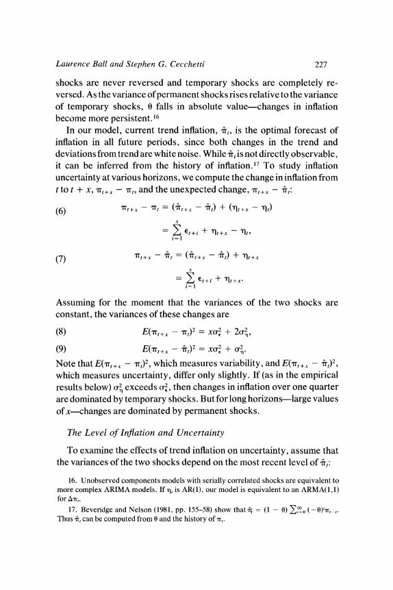
Laurence Ball and Stephen G. Cecchetti 227
shocks are never reversed and temporary shocks are completely re- versed. As the variance of permanent shocks rises relative to the variance of temporary shocks, 0 falls in absolute value-changes in inflation become more persistent. 16
In our model, current trend inflation, *,rt, is the optimal forecast of inflation in all future periods, since both changes in the trend and deviations from trend are white noise. While *,r is not directly observable, it can be inferred from the history of inflation.17 To study inflation uncertainty at various horizons, we compute the change in inflation from t to t + x, 'rt +x - t, and the unexpected change, rr+X t -*,:
(6) wt+X - ' = (t.+x - *t) + (t+x - t)
x
= E Et+i + t+X - Tit,
(7) -*t = (*r+ - rXt) + Tqt+X
x
=Ets+i + Tlt+x. i= 1
~X
Assuming for the moment that the variances of the two shocks are constant, the variances of these changes are
(8) E(-Tt+x -t)2 = Xo-2 + 2C2,
(9) EQrr,+X - -fr)2 = XCz2 + C2
Note that E(,Tt+x - X,)2, which measures variability, and E(Qr+W -* which measures uncertainty, differ only slightly. If (as in the empirical results below) C2 exceeds C2, then changes in inflation over one quarter are dominated by temporary shocks. But for long horizons-large values of x-changes are dominated by permanent shocks.
The Level of Inflation and Uncertainty
To examine the effects of trend inflation on uncertainty, assume that the variances of the two shocks depend on the most recent level of *,>:
16. Unobserved components models with serially correlated shocks are equivalent to more complex ARIMA models. If q, is AR(1), our model is equivalent to an ARMA(1, 1) for As,.
17. Beveridge and Nelson (1981, pp. 155-58) show that*i, = (1 - 0) E ?-? (-0)i7',- . Thus -f, can be computed from 0 and the history of a,.

228 Brookings Paper-s on Economic Activity, 1:1990
(10) o2 (t) = po + 3 It- ;
(11) CoE(t) = Io ? 8rft-l
This paper's basic hypothesis is that trend inflation has a stronger effect on cr than on a,,. In terms of the equivalent IMA(1, 1) model, a high trend makes changes in inflation more persistent. A strong effect of trend inflation on Cr means that the trend is less stable when it is high-as suggested by Okun and Ball, high inflation makes the Federal Reserve more likely to disinflate or to allow inflation to rise further. A weak effect on a,, means that high inflation does not greatly increase monetary control errors, fluctuations in money demand, or other sources of temporary movements in inflation.
If our hypothesis is true, then it explains our preliminary finding that inflation has larger effects on uncertainty at longer horizons. To see this, substitute equations 10 and 11 into equation 9 to compute uncertainty about inflation conditional on the current trend:
(12) E[('rrt+x - frt)2[$t] =x(PO + P3*ft) + (80 + 81 rft)
(The variances of future shocks conditional on *,rt are the same as the variances of current shocks, because the best forecast of future *a's is the current *a.) The effect of an increase in *,r is given by
(13) = -frt) I*r] - Xp + 81. ditr
If PI is large and 81 is small-*, has a larger effect on the variance of permanent shocks-then *,r has a much larger effect on uncertainty at long horizons.
Main Results
Here we present our main empirical findings. We estimate our statistical model and examine the relations between the level of inflation and the variances of the two shocks. We estimate these relations both across countries and over time, and we consider both moderate- and high-inflation countries.
In principle, one could estimate our model with a time series for one country and allow the variances to change over time according to

Laurence Ball and Stephen G. Cecchetti 229
equations 10-11. This approach would produce estimates of PI and 81, the effects of *,r on the variances.18 The econometrics of this approach are complicated, however, and so we leave it for future work. Here we proceed in two simpler ways. First, we assume that the two variances are constant for a given country and estimate the cross-country relation between the variances and average inflation. Second, we divide each country's data into five-year periods and estimate the relation between the variances and average inflation across periods.
We use quarterly, seasonally adjusted data on the CPI and either the GNP or the GDP deflator.19 The CPI data, from the International Monetary Fund's InternationalFinancial Statistics and the Organization for Economic Cooperation and Development, cover 40 countries. The deflator data, from the OECD, cover 9 countries. For each country we use data from 1960:2 (or the beginning of the sample, where that is later) to the most recent quarter available (usually 1989: 1). When we divide the data into five-year periods, we have six periods beginning in 1984:2, 1979:2, and so on.20
Table 3 lists the countries in our sample and, for each country, the years for which data are available. The table also shows the means and simple standard deviations of quarterly inflation. The countries vary widely in their inflation experiences. Average quarterly inflation is less than 2 percent in many European and North American countries, but exceeds 10 percent in Israel and several South American countries.
Before estimating our model, we check whether it fits the data. For 38 of 40 countries, Dickey-Fuller tests on CPI data fail to reject at the 10 percent level our assumption that inflation is nonstationary.21 To test our assumption that both permanent and temporary inflation shocks are white noise, we compare the implied MA(1) model for &Tr, with more
18. See Evans (1989) for a related approach to measuring time variation in short-run and long-run inflation uncertainty.
19. The deflator data are seasonally adjusted by the OECD. We seasonally adjust the CPI by regressing unadjusted quarterly inflation on quarter dummies and using the residuals.
20. The first period is four years (1960:2 to 1964:1). In addition, because the beginning and end of the sample vary across countries, we sometimes have data for only part of a period. We include a period for a given country if we have inflation data for at least 12 quarters.
21. We perform the augmented Dickey-Fuller tests described in section 5 of Dickey and Fuller (1981).

230 Brookings Papers on Economic Activity, 1:1990
Table 3. Quarterly Inflation, Mean and Standard Deviation, Sample of 40 Countries, 1960-89
Consulmer price index GNP deflator
Mean Standard Mean Standard Country Sample inflation deviation Sample inflation deviation
Argentinaa 1970:1 to 1987:4 28.96 562.48 ... ...
Australia 1960:1 to 1988:4 1.69 1.19 1960:1 to 1988:4b 1.79 1.35 Austria 1960:1 to 1989:1 1.11 1.31 .. . ...
Belgium 1960:1 to 1989:2 1.22 0.96 ... ... ... Boliviaa 1970:1 to 1987:4 29.67 5,090.38 . . .. .
Brazila 1964:1 to 1988:2 15.64 381.37 ... ... ... Canada 1960:1 to 1989:1 1.36 0.89 1961:1 to 1989:1 1.39 0.90 Chilea 1970:1 to 1987:4 16.30 416.21 ... ... Colombiaa 1964:1 to 1988:2 4.35 7.59 ... ... Denmark 1960:1 to 1989:1 1.79 1.27 ... ....
Dominican Republica 1964:1 to 1987:3 2.28 10.97 ... ... ... Ecuadora 1964:1 to 1988:2 2.59 6.64 ... ... ... El Salvadora 1964:1 to 1988:2 3.79 12.82 ... ... ... Finland 1960:1 to 1989:1 1.87 1.78 ... ....
France 1960:1 to 1989:1 1.64 1.02 1971:1 to 1988:4b 2.06 0.88
Great Britain 1960:1 to 1989:1 1.94 1.54 1960:1 to 1989:lb 1.98 1.63 Greece 1960:1 to 1989:1 2.71 2.42 ... ...
Guatemalaa 1964:1 to 1987:4 2.00 11.92 ... ... Ireland 1960:1 to 1988:4 2.16 1.77 ... ....
Israela 1964:1 to 1988:2 11.50 190.92 ... ... .
Italy 1960:1 to 1989:1 2.22 1.58 1960:1 to 1988:2b 2.38 1.66 Jamaicaa 1964:1 to 1988:2 3.14 9.58 ... ...
Japan 1960:1 to 1989:1 1.39 1.43 1965:1 to 1989:1 1.18 1.24 Luxembourg 1960:1 to 1989:1 1.12 0.93 ... ... ... Mexicoa 1964:1 to 1988:2 7.05 60.45 . . . . ..
Netherlands 1960:1 to 1989:1 1.14 1.05 ... ... New Zealand 1960:1 to 1984:2 2.08 1.38 ... ... Norway 1960:1 to 1989:1 1.68 1.60 ... ....
PerUa 1964:1 to 1988:1 9.97 91.55 ... ... Philippinesa 1964:1 to 1988:2 2.99 11.70 ... ... ...
Portugal 1960:1 to 1989:1 3.10 2.81 ... ... ... Singaporea 1968:1 to 1988:2 0.99 4.76 ... ... ... South Africaa 1964:1 to 1988:2 2.42 1.84 ... ... ... Spain 1960:1 to 1989:1 2.44 1.82 ... ... ... Sweden 1960:1 to 1989:1 1.65 1.10 ... ... ...
Switzerland 1960:1 to 1989:1 0.95 0.85 1967:1 to 1989:lb 1.11 1.09 Turkey 1960:1 to 1989:1 6.15 7.10 ... ... ... United States 1960:1 to 1989:1 1.24 0.92 1960:1 to 1989:1 1.22 0.72 Venezuelaa 1964:1 to 1988:2 2.12 5.13 ... ... ... West Germany 1960:1 to 1989:1 0.87 0.66 1960:1 to 1989:1 0.98 0.79
Sources: Data for countries in Central and South America, the Caribbean, Israel, the Philippines, Singapore, and South Africa are from International Monetary Fund, International Finiancial Statistics, spliced from tape and various editions. All other data are from OECD, Maini Econonmic Itndicators, 1989 edition. Data are quarterly and seasonally adjusted.
a. IMF data. b. GDP deflator.

Laurence Ball and Stephen G. Cecchetti 231
general models. For each country we estimate all ARMA(p, q) models for p c 2 and 0 < q c 2 and choose among them using the Schwarz criterion (which maximizes the likelihood function with penalties for extra parameters).22 We choose an MA(1) in 32 of 40 cases for the CPI and 5 of 9 cases for deflators; the other countries are mainly MA(2). Finally, for U.S. data we use the same procedure to choose models for As,rt in the 1960s, 1970s, and 1980s. For deflator data, the Schwarz criterion chooses an MA(1) for all three periods; for the CPI, it chooses an MA(1) for the 1970s and 1980s and an MA(2) for the 1960s. These results suggest that our model is a good approximation to the behavior of inflation in a wide range of circumstances. For simplicity, our main analysis assumes that our model always holds, but we experiment with relaxing this assumption.23
For a given country or period, we estimate the variances of the two errors in equations 1 and 2 by maximum likelihood. Specifically, we use the approach of Andrew Harvey to estimate an MA(1) model for Awrt and then use equation 5 to work back to the two variances.24
We begin by considering the experience of the United States. We then extend the analysis to a sample of 28 moderate-inflation countries (average quarterly inflation below 3 percent). For this sample, we check the robustness of our results as well as estimating the basic model. Finally, we ask whether the results extend to the 12 high-inflation countries in our data set.
The United States
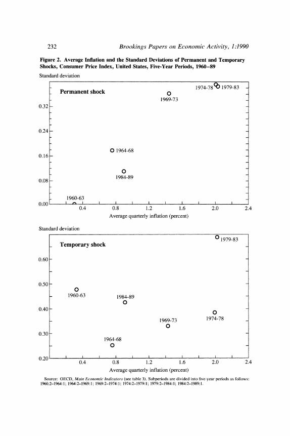
For U.S. CPI data, figure 2 plots average inflation for the six five-year periods against our estimates of the standard deviations of the two shocks. For both the CPI and the GNP deflator, table 4 reports the
22. Schwarz (1978) suggests minimizing - 21n 2 + (p + q)lnT, where 2 is the likelihood value for the model, T is the sample size, and p and q are the number of AR and MA parameters, respectively.
23. We also investigate the possibility that there are regime shifts in inflation that cannot be captured by an ARIMA model. We consider a process switching model with both normal and extraordinary shocks to inflation; see, for example, Friedman and Laibson (1989) and Cecchetti, Lam, and Mark (1990). Such a model would be indicated by excess kurtosis in the distribution of changes in inflation. Diagnostic tests on U.S. data provide no evidence of excess kurtosis.
24. Harvey (1981).
232 Brookings Papers on Economic Activity, 1:1990
Figure 2. Average Inflation and the Standard Deviations of Permanent and Temporary Shocks, Consumer Price Index, United States, Five-Year Periods, 1960-89
Standard deviation
~~~~~~~~ ~~~~~~1974-78 9 1979-83 _ Permanent shock O
1969-73 0.32 -
0.24 -
0 1964-68 0.16 -
0
0.08 _ 1984-89
1960-63 0.00 I I I I I I I
0.4 0.8 1.2 1.6 2.0 2.4
Average quarterly inflation (percent)
Standard deviation
0 1979-83 _ Temporary shock
0.60 -
0.50 _ 0
_ 1960-63 1984-89 0
0.40 -
1969-73 1974-78 _ 0
0.30 - _ 1964-68
0
0.20 1 I l l
I I l
0.4 0.8 1.2 1.6 2.0 2.4
Average quarterly inflation (percent)
Source: OECD, Main Economic Indicators (see table 3). Subperiods are divided into five-year periods as follows: 1960:2-1964: 1; 1964:2-1969: 1; 1969:2-1974: 1; 1974:2-1979: 1; 1979:2-1984: 1; 1984:2-1989: 1.

Laurence Ball and Stephen G. Cecchetti 233
Table 4. Effects of Average Inflation on the Standard Deviations of Permanent and Temporary Shocks, United States, Five-year Periods, 1960:2-1989:1
Coefficient on average
Dependent variable inflation R2
Consumer price index Permanent shock (crj 0.230 0.897
(10.80) Temporary shock (cra) 0.081 0.137
(0.88)
GNP deflator Permanent shock (a) 0.159 0.864
(6.87) Temporary shock (v,,) - 0.005 0.001
(-0.07)
Source: OECD, Main Ecotionoic Indicators. Numbers in parentheses are t-statistics.
results of simple regressions of each standard deviation on average inflation (with heteroskedasticity-consistent standard errors). Experi- mentation shows that linear relations between the standard deviations and average inflation fit better than ones between variances and average inflation.
Although our regressions use only six observations, the results are clear. For both the CPI and the deflator, the effect of average inflation on the standard deviation of permanent shocks is positive and highly significant. Indeed, the R2's are close to 0.9: differences in average inflation explain almost all the variation in ,e. In contrast, there is no evidence that average inflation affects o-,: the coefficient estimates are small and the t-statistics are less than one.
It is interesting to examine the details of the U.S. experience. As shown in figure 2, high average inflation in 1979-83 was accompanied by large variance in both the permanent and temporary components of inflation. The former is likely explained by the Volcker disinflation and the latter by fluctuations in food and energy prices.25 The two other high- inflation periods, 1969-73 and 1974-78, also have large permanent
25. Blinder (1982).

234 Brookings Papers on Economic Activity, 1:1990
shocks. Likely culprits include disinflations begun in December 1968 and April 1974, and the Federal Reserve's inflationary response to the 1975 recession.26 In these two periods, however, the variances of temporary shocks are fairly low. There were larger temporary shocks in the low-inflation periods of 1960-63 and 1984-89. In those periods, trend inflation was stable, but short-term fluctuations arose from macroeco- nomic shocks (recession and recovery in the early 1960s; the favorable oil shock in 1986). During the past 30 years of U. S. history, high inflation has always been accompanied by shifting monetary policy, and hence an unstable trend. But temporary inflation shocks can occur at either high or low inflation.
We can use our regression results to calculate the effects of average inflation on uncertainty over various horizons. Our fitted relations between average inflation and the two standard deviations imply qua- dratic relations between average inflation and the two variances. We first linearize these relations around the sample mean of average infla- tion.27 We then use the parameters of the linear relations to compute the ratio of equation 13 to equation 12-the percentage increase in uncer- tainty per percentage point increase in trend inflation-starting at the sample mean. We also compute standard errors for these effects. For the deflator, the effect forx = 1 is 32 percent (t = 0.9). The point estimate implies that a 1 point rise in quarterly trend inflation raises uncertainty about next quarter's inflation by 32 percent, but the effect is statistically insignificant. The effect rises to 143 percent (t = 9.2) at x = 10 and 174 percent (t = 8.5) at x = 20, and approaches 221 percent (t = 6.9) as x approaches infinity. (As x approaches infinity, both equations 12 and 13 approach infinity, but their ratio remains finite.) For the CPI, the effect is 74 percent (t = 2.5) at x = 1. It rises to 171 percent (t = 14) at x = 20 and 192 percent (t = 11) as x approaches infinity. For the CPI, inflation has statistically significant effects on uncertainty at all horizons, but the effects are much larger at long horizons.
26. Romer and Romer (1989). 27. Alternatively, we could assume a quadratic relation between -*, and the variances
and derive modified versions of equations 12 and 13. In this case, we can use the exact relations implied by our regressions rather than linearizing them. This approach is complicated, however, and experimentation shows that the results are almost the same.

Laurence Ball and Stephen G. Cecchetti 235
Moderate-Inflation Countries: Basic Results
We now extend our analysis to international data. We begin by considering the 28 countries with average quarterly inflation below 3 percent. Here we estimate our basic model with CPI data; later we explore the effects of generalizing the model and of using deflator data where it exists.
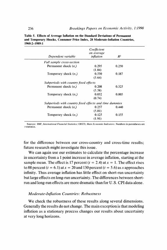
We first examine the cross-country relation between inflation and uncertainty. For each country, we assume that u-. and u, are constant and estimate them for the entire post-1960 period. The top panel of table 5 reports the results of regressing the estimated standard deviations on average inflation for the entire period. These results do not support our hypothesis that average inflation affects u, but not u',. Instead, the t-statistic for average inflation is 1.8 in the u-e regression and 3.6 in the u-, regression, and in both cases the coefficients imply large effects.
Next we examine the relation between inflation and uncertainty over time. We estimate the two standard deviations for five-year periods in each country, and use the resulting country-period panel data to estimate the effect of average inflation on each standard deviation. In both regressions, we include country-specific fixed effects to isolate the effects of changes in inflation over time. That is, we estimate
(14) Ue(i, t) = c-i + 1 ri .,
(15) oX,(i, t) = 'y + 81i Tit,
where i indexes countries, t indexes periods, and ri, is average inflation for country i in period t. The middle panel of table 5 reports regression results similar to the U.S. results reported above. The effect of average inflation on uE is both statistically and economically significant, while the effect on u-, is small and statistically insignificant.
Thus the relation between inflation and uncertainty is different across countries and over time. A relatively high-inflation country like Greece experiences both greater instability in trend inflation (a higher oE) and greater fluctuations around trend (a higher u,) than a low-inflation country like West Germany. For a given country, a rise in trend inflation from one period to the next makes the trend less stable but does not affect fluctuations around the trend. We do not have a clear explanation
236 Brookings Papers on Economic Activity, 1:1990
Table 5. Effects of Average Inflation on the Standard Deviations of Permanent and Temporary Shocks, Consumer Price Index, 28 Moderate-Inflation Countries, 1960:2-1989:1
Coefficient on average
Dependent variable inflation R2
Full sample cross-section Permanent shock (a) 0.295 0.250
(1.84) Temporary shock (v,,) 0.530 0.187
(3.64)
Subperiods with country fixed effects Permanent shock (a) 0.208 0.325
(5.58) Temporary shock (v,,) 0.032 0.005
(0.74) Subperiods with country fixed effects and time dummies
Permanent shock (a) 0.257 0.440 (5.81)
Temporary shock (v,,) 0.125 0.155 (1.91)
Sources: IMF, Internationial Finianicial Statistics; OECD, Maini Ecotionmic Indicators. Numbers in parentheses are t-statistics.
for the difference between our cross-country and cross-time results; future research might investigate this issue.
We can again use our estimates to calculate the percentage increase in uncertainty from a 1 point increase in average inflation, starting at the sample mean. The effect is 17 percent (t = 2.4) at x = 1. The effect rises to 88 percent (t = 6. 1) atx = 20 and 130 percent (t = 5.6) as x approaches infinity. Thus average inflation has little effect on short-run uncertainty but large effects on long-run uncertainty. The differences between short- run and long-run effects are more dramatic than for U.S. CPI data alone.
Moderate-Inflation Countries: Robustness
We check the robustness of these results along several dimensions. Generally the results do not change. The main exception is that modeling inflation as a stationary process changes our results about uncertainty at very long horizons.

Laurence Ball and Stephen G. Cecchetti 237
We first estimate our equations with fixed effects for time periods as well as countries; that is, we add dummy variables for periods to equations 14 and 15. Our basic panel results could be driven by one or two events, such as the supply shocks of the 1970s, that had similar effects on inflation in many countries.28 By including time dummies, we isolate the effects of idiosyncratic changes in inflation in the 28 countries. As shown in the bottom of table 5, including these dummies has little effect on the coefficients on average inflation. In the same spirit, we also estimate equations 14 and 15 separately for the 1960s, 1970s, and 1980s (each decade has two observations per country). For both equations, we cannot reject the hypothesis that the average inflation coefficient is constant across decades.29
We also relax the assumption that the temporary shock t is white noise in all countries. For each country, we test our MA(1) model for &,ut against the ARMA(1,1) model that arises when -q, is AR(1). For 3 out of 28 countries, a likelihood ratio test rejects the MA(1) model at the 5 percent level. For these countries, we assume that t is AR(1) and estimate uE and u, with a generalization of our basic procedure. We then repeat our cross-country and cross-time regressions using the new standard deviations for the three countries. Not surprisingly, the results are almost identical to those in table 5.
Next, we consider the possibility that trend inflation follows a highly persistent but stationary process. We assume that *,r is AR(1), so our model becomes
(16) '
1* = L + P*t- I + Et,
28. Taylor (1981) suggests that the supply shocks of the 1970s raised both average inflation and variability.
29. We also reestimate equations 14 and 15 for the whole sample using inflation at the start of a period rather than average inflation over the entire period as the independent variable. (More precisely, we use inflation over the first two quarters of the period and the last two quarters of the previous period.) Panel members have suggested that outbreaks of inflation in certain periods may cause average inflation and r. to move together even if the level of inflation does not affect uncertainty. Using start-of-period inflation reveals whether high inflation at a point in time implies greater uncertainty about the future. Empirically, the distinction proves unimportant. Using start-of-period inflation in equa- tions 14 and 15 produces coefficients of 0. 10 (t = 2.8) for a, and - 0.02 (t = 0.5) for o,.

238 Brookings Papers on Economic Activity, 1:1990
where E and -q, are white noise. In this case, the level of inflation -r, follows an ARMA(1, 1); estimating this process allows us to work back to equation 16. For almost all countries, estimates of p range from 0.90 to 0.99. To measure the inflation-uncertainty relation, we impose p = 0.95 for all countries and periods and estimate oE and u',. Panel regressions of the standard deviations on average inflation yield coefficients of 0. 170 (t = 4.3) foroTE and 0.034 (t = 1.1) for u',. These results are close to those in the middle panel of table 5.
For our stationary model, we combine the regression results with generalizations of equations 12 and 13 to estimate the effects of inflation on uncertainty at various horizons. For short and moderately long horizons, the results are similar to those for our basic model. As the horizon becomes very long, however, the effects peak and then decline rather than rising monotonically. A 1 point rise in average inflation raises uncertainty by 16 percent at x = 1, by 36 percent at x = 10, by 29 percent at x = 20, and by only 8 percent at x = 50. This hump shape is similar to the correlations between ut and (Ut+" - X,)2 in figure 1. These results should be interpreted cautiously, however, because it is difficult to distinguish between our stationary and nonstationary models. The effects of inflation on uncertainty clearly rise as we move from short to moderately long horizons, but we cannot draw firm conclusions about very long horizons.
Finally, for our basic model, table 6 reports results for data on deflators. The cross-country results, which are based on nine observa- tions, are inconclusive.30 Panel results with country-specific fixed effects are quite similar to the corresponding results for the CPI.
High-Inflation Countries
We now consider our full sample of 40 countries, which includes 6 countries with average quarterly inflation above 10 percent. In principle, the inflation-uncertainty relation could be quite different in high- and moderate-inflation countries, because inflation in the former depends on factors that are unimportant in the latter, such as the need for seignorage
30. The coefficients on inflation in the deflator regressions are smaller than those in the CPI regressions. But when we restrict the CPI sample to the nine countries for which we have deflator data, the two inflation measures produce similar results.

Laurence Ball and Stephen G. Cecchetti 239
Table 6. Effects of Average Inflation on the Standard Deviations of Permanent and Temporary Shocks, GNP Deflator, Nine Countries, 1960:2-1989:1
Coefficient on average
Dependent variable inflation R2
Full sample cross-section Permanent shock (a) 0.127 0.204
(1.67) Temporary shock (v,,) 0.137 0.073
(1.02)
Subperiods with country fixed effects Permanent shock (a) 0.222 0.503
(4.74) Temporary shock (v,,) 0.059 0.035
(1.23)
Subperiods with countiy fixed effects and time dummies Permanent shock (a) 0.200 0.583
(3.30) Temporary shock (v,,) 0.046 0.273
(0.76)
Source: OECD, Main Economic Indicators. GDP deflator is used for Australia, France, Great Britain, Italy, and Switzerland. Numbers in parentheses are t-statistics.
revenue. We find, however, that the qualitative relations between inflation and uncertainty are similar.
Table 7 reports our basic cross-country and panel regressions for the full sample. Across countries, average inflation again has a sizable effect on both uS and u,. In the cross-time regressions, average inflation has a large effect on UE. The effect on u. now borders on statistical significance (t = 1.6 without time dummies, t = 2.3 with time dummies), but the coefficient is small. Results for the 12 high-inflation countries alone, which are reported in table 8, are similar to the results for all 40 countries. In high-inflation countries, a rise in inflation over time raises both Se and U., but the effect on u, is weak.
The effects of average inflation on Se are somewhat larger for high- inflation countries than for moderate-inflation countries; for example, the coefficients in the middle panels of tables 8 and 5 are 0.39 and 0.21, respectively. Since these results suggest some nonlinearity, we add average inflation squared to our equations for the full sample. The squared terms appear to belong in the panel regressions but not in the simple cross-country regressions. In the panel regression for Ie, the

240 Brookings Paper-s on Economic Activity, 1:1990
Table 7. Effects of Average Inflation on the Standard Deviations of Permanent and Temporary Shocks, Consumer Price Index, Full Sample, 1960:2-1989:1
Coefficient on average
Dependent variable inflation R2
Full sample cross-sectiona Permanent shock (a) 0.395 0.869
(7.21) Temporary shock (v,,) 0.501 0.705
(4.38)
Subperiods with country fixed effects Permanent shock (r,) 0.382 0.798
(11.94) Temporary shock (an) 0.092 0.054
(1.59)
Subperiods with country fixed effects and time dummies Permanent shock (a) 0.399 0.832
(12.98) Temporary shock (rfn) 0.131 0.112
(2.28)
Sources: IMF, Internzational Finianicial Statistics; OECD, Main Econiomic Indicators. Numbers in parentheses are t-statistics.
a. Full sample cross-section regressions exclude Bolivia. Panel regressions exclude period including 1985-86 Bolivian hyperinflation.
coefficients on average inflation and its square are 0.22 and 0.005. These results imply that a 1 point rise in average inflation raises uS by 0.23 if the average is initially 1 percent, and by 0.37 if the average is initially 15 percent. Thus the effect of inflation on uncertainty becomes somewhat stronger as inflation rises.
Extensions
In the next two sections we report on extensions of our basic analysis that test the robustness of our results.
An Alternative Measure of Core Inflation
Our central finding is that a higher trend rate of inflation raises the variance of the trend but not the variance of deviations from trend. This finding depends, of course, on our method for decomposing movements in inflation into shifts in trend and deviations from trend. We now try a

Laurence Ball and Stephen G. Cecchetti 241
Table 8. Effects of Average Inflation on the Standard Deviations of Permanent and Temporary Shocks, Consumer Price Index, 12 High-Inflation Countries, 1960:2-1989:1
Coefficient on average
Dependent variable inflation R2
Full sample cross-sectiona Permanent shock (a) 0.420 0.805
(6.39) Temporary shock (v,,) 0.507 0.568
(3.61)
Subperiods with countr-y fixed effects Permanent shock (a) 0.389 0.820
(11.79) Temporary shock (v,,) 0.094 0.058
(1.57)
Suibperiods with countly fixed effects and time dummies Permanent shock (ok) 0.418 0.866
(13.74) Temporary shock (v,,) 0.197 0.204
(2.88)
Sources: IMF, Initernzationial Finanicial Statistics; OECD, Maini Econiomizic Itndicators. Numbers in parentheses are t-statistics.
a. Full sample cross-section regressions exclude Bolivia. Panel regressions exclude period including 1985-86 Bolivian hyperinflation.
completely different approach to this decomposition. Following Alan Blinder and others, we define core inflation as the CPI excluding food and energy.3" The idea behind this definition is that movements in food and energy prices largely reflect transitory effects of weather and OPEC decisions, so that excluding them provides an inflation measure that more nearly reflects the trend.
We now test our basic hypothesis about trend and deviations using this direct measure of core inflation. Let
(17) m= ,Tt F
(18) ~ ~ ~ ~ E ,= Wc - '7c_
where wrrc is core inflation. The variables & and ft are our new measures of changes in trend inflation and deviations from trend. We estimate
31. See Blinder (1982). Journalists often report the CPI excluding food and energy as a measure of trend inflation.

242 Brookings Papers on Economic Activity, 1:1990
(19) I 'J = %o + , Trc + u1
(20) E't = o + PB 'rr + u2t.
That is, we estimate the effects of core inflation on the absolute sizes of the two shocks. For quarterly U.S. data for 1960-88, the estimates of 13 and 8, with t-statistics using Newey-West standard errors are 0.206 (t = 3.9) and 0.019 (t = 1.2).32 A rise in core inflation has a sizable effect on fluctuations in the trend and a small effect on deviations. These results confirm the message of the previous section.33
Variability and Uncertainty
As discussed above, Fischer and others emphasize the distinction between inflation variability and inflation uncertainty. It is possible that when inflation is high it varies considerably, but that the movements are largely predictable, so the variance of unanticipated inflation is not especially large. In our model, this distinction is unimportant: for a given horizon, the variances of the change in inflation and the unanticipated change are similar (see equations 8 and 9). A major limitation of our model, however, is that it is univariate. When inflation is high, its movements might be unpredictable in a univariate model, but largely predictable based on other variables. If, for example, inflation variability arises from unstable monetary policy, lagged money growth could have considerable predictive power. Engle measures uncertainty with a multivariate model. Could this help explain why he finds no effect of inflation on uncertainty?
In principle, one could estimate a multivariate version of our statistical model. In such a framework, both temporary and permanent changes in inflation would depend on lagged values of observable variables. This approach is difficult, however, and so we take a simpler one. We extend our preliminary calculations of correlations between the level of inflation and squared changes at various horizons. Here, we first regress the change from t to t + x on a vector of variables known at t:
32. A direct measure of core inflation is available only for the United States. We use the technique of Newey and West (1987) with five lags.
33. The sample variances of i, and Et are 0.080 and 0.336, respectively. In our unobserved components model, r2 exceeds U2. These results suggest that the food and energy shocks captured by i, are only part of the temporary fluctuations in inflation.

Laurence Ball and Stephen G. Cecchetti 243
Table 9. Correlations of Inflation with Squared Change and Squared Unanticipated Change in Inflation, United States, 1954-89
Correlation
GNP deflator CPI
Horizon in Unanticipated Actual Unanticipated Actual quarters (x) changea changeb changea changeb
1 0.148 0.086 0.192 0.213 2 0.164 0.134 0.335 0.395 3 0.151 0.121 0.217 0.333 4 0.169 0.192 0.298 0.376 5 0.274 0.357 0.295 0.412
6 0.220 0.313 0.256 0.405 7 0.177 0.304 0.353 0.439 8 0.182 0.344 0.311 0.447 9 0.105 0.207 0.266 0.410
10 0.172 0.303 0.319 0.422
12 0.259 0.366 0.408 0.470 14 0.403 0.416 0.485 0.530 16 0.287 0.282 0.456 0.491 18 0.322 0.323 0.588 0.602 20 0.339 0.355 0.560 0.572
24 0.361 0.211 0.600 0.514 28 0.247 0.133 0.469 0.396 32 0.256 0.197 0.380 0.383 36 0.267 0.201 0.365 0.279 40 0.249 0.055 0.324 0.162
44 0.297 - 0.005 0.440 0.127 48 0.282 -0.071 0.423 0.153 50 0.326 -0.045 0.311 0.016
Source: Citibase. Quarterly data, seasonally adjusted, for implicit GNP deflator and CPI-U for all items. a. Correlation of inflation with the square of the residual from equation 21 in the text. b. Correlation of inflation with the square of the actual change in inflation. Also shown in table 2.
(21) 1Tt+x - =t = Zty.,y + ex,
where Zt is information available at t and yx is a vector of coefficients. The residuals from this regression, ex ,, capture the unanticipatedchange in inflation-the part not predictable from the Z's. We measure the relation between inflation and uncertainty by the correlation between 7Ft and the squared residuals.
For U.S. data for 1954-89, table 9 reports results when Z includes four lags of each of three variables: the change in inflation, the change in M2 growth, and real output growth. (The results are robust to adding

244 Brookings Papers on Economic Activity, 1:1990
changes in wage growth and changes in import price inflation, both used by Engle.) The table compares the correlations between wr, and the squared residuals from equation 21 with the correlations between -r, and the squared change in inflation, which were presented in table 2. The results are quite similar: the level of inflation has similar effects on the size of changes and the size of unanticipated changes. The results again show the importance of horizons, and suggest that the uncertainty- variability distinction is not important.34
Conclusion
This paper investigates the relation between inflation and uncertainty at short and long horizons. We decompose movements in inflation into shifts in trend inflation and temporary deviations from trend. Uncertainty about next quarter's inflation depends mainly on the variance of devia- tions, while uncertainty about inflation over several years depends mainly on the variance of the trend. We find that a rise in the level of inflation has little effect on the variance of deviations, but makes the trend considerably less stable. Thus inflation has much larger effects on uncertainty at long horizons.
Because trend inflation is determined by monetary policy, our results suggest that high inflation makes policy less stable. This conclusion fits the U.S. experience during the 1970s. Fearing unemployment, the Federal Reserve initially accommodated the oil and food shocks of 1973, but the alarming rise in inflation led to tighter policy in 1974. Inflation dropped, but the deep recession of 1975 produced another loosening of policy. A similar pattern of accommodation and then reversal followed the supply shocks of the late 1970s. As Okun predicted in 1971, high inflation led to 'stop-go' policies. In contrast, the relatively low inflation of the 1980s has produced steady policy aimed at keeping inflation low.35
Our finding that high inflation raises long-run uncertainty implies that
34. The R2's from estimating equation 21 are substantial. For the CPI, the R2 is 0.42 for x = 1, 0.33 for x = 10, and 0.16 for x = 40. Thus variables such as money growth and output do help forecast inflation. But variability in the unforecastable part has a similar relation to the level of inflation as total variability.
35. For the history of inflation in the 1970s, see Blinder (1982) and Romer and Romer (1989).

Laurence Ball and Stephen G. Cecchetti 245
inflation has substantial costs. Two costs of unstable trend inflation are perhaps most important. First, as emphasized by Milton Friedman, uncertainty creates risk for individuals with nominal contracts such as loans, pensions, and labor contracts. This risk reduces the efficiency gains from these arrangements and individuals' willingness to enter them. Second, the stop-go monetary policy that produces unstable inflation also produces unstable output. Policy swings that create reces- sions, such as the drastic tightening in 1979, are usually a reaction to high inflation.
A possible policy implication is that the Federal Reserve should fight inflation. If OPEC III occurs this year, Alan Greenspan should realize that accommodating it will lead not only to a high level of inflation but also to costly uncertainty. Of course, failing to accommodate the shock will lead to high unemployment, which is also costly. As Okun empha- sized, there is no easy solution to the output-inflation trade-off.
On the other hand, our results suggest that the trade-off can be made somewhat less painful. Because costly uncertainty arises from unstable policy, the Federal Reserve can reduce the costs by making policy more stable. If Alan Greenspan does accommodate OPEC III, then he and his successors should avoid a stop-go reaction to the resulting inflation. It might be desirable, for example, to make a well-publicized commitment to gradual disinflation. Such commitments are most important at high inflation, where our results suggest that the danger of unstable policy is greatest. At low inflation, policy tends naturally to be stable even under discretion.36
36. Our discussant takes this point a step further and suggests that the Federal Reserve simply stabilize inflation at its current level rather than disinflate. With a firm commitment to stability, the costs of inflation might be small. We find this idea interesting, but we are skeptical. Our empirical results are robust: across a wide variety of countries and periods, higher trend inflation is almost always accompanied by greater variation in the trend. High but steady inflation may be possible in theory, but it is very rare in practice. Why is it hard to stabilize inflation at a high level? Okun and Fischer and Summers (1989) argue that inflationary expectations rise considerably if the public believes that the Federal Reserve has given up the fight against inflation. The Federal Reserve must then accommodate these expectations to avoid a recession; the result is not stable inflation but a rise to a higher level. Another complication is that a Federal Reserve decision to live with inflation could be thwarted by pressure from politicians or Wall Street. High inflation creates political controversy, and political controversy produces stop-go policies. (Imagine the reaction if Paul Volcker had announced in 1979 that he would accept double-digit inflation forever.)

Comments and Discussion
Robert J. Gordon: Laurence Ball and Stephen Cecchetti present a technically sophisticated treatment of an old and familiar question, the relationship between the mean rate of inflation and the variability of inflation. Before dipping into the core of the paper, with its many excellent ideas and details of execution, let's step back and review the basic policy dilemma that motivates the entire enterprise.
Today, as at the first meeting of the Brookings Panel in 1970, the inflation rate is about 5 percent. The policymaker would prefer zero inflation, but is presented with extremely convincing research that the economy is subject to a non-zero sacrifice ratio, that is, the percentage of one year's real GNP that must be sacrificed permanently to reduce inflation by 1 percentage point. The sacrifice ratio for the disinflation of the 1980s was predicted in advance to be about six, and indeed turned out to be almost exactly that.1 Most people now agree that losing 6 percent of a year's GNP is almost entirely a true loss, with little offset from an increased value of leisure.
But there is wide disagreement about what, if any, gain society enjoys from a 1 point permanent reduction of the inflation rate. The traditional money-triangle analysis always yielded low numbers. This approach yields an even smaller benefit of reduced inflation now, as the fraction of the money supply paying interest is much higher than it was 10 years ago, and the monetary base that pays no interest has fallen to less than 6 percent of GNP. The inadequacy of the money-triangle approach has long been summed up by saying that "it takes a heap of Harberger
1. Gordon and King (1982, table 5, line 3). Reasons for preferring the line 3 variant are given on pp. 236-37.
246

Laurence Ball and Stephen G. Cecchetti 247
triangles to fill an Okun gap." This recognition set the opponents of inflation off on a different tack in their search for its welfare costs.
Ironically it was Arthur Okun himself, the father of the gap, who has the earliest cited article on the Ball-Cecchetti reference list, making the point that there is a positive correlation between the mean and variance of inflation. The implication is that the main welfare cost of high mean inflation is a high variance of inflation, with all the classic redistribution among creditors and debtors that occurs with a variable inflation rate. In 1971 I wrote a short BPEA report that accepted Okun's premise but disputed his empirical results as being dependent on the inclusion of a few high-inflation countries. Today Ball and Cecchetti, with two decades of evidence and better techniques, support Okun in that debate.
So let me accept that there is a positive relationship between the mean and variance even for moderate-inflation countries and instead offer a deeper objection to this line of research: it is simply irrelevant to the policy problem of assessing the trade-off between the social costs and benefits of disinflation. As the authors recognize, too late, in their last paragraph, "Because costly uncertainty arises from unstable policy, the Federal Reserve can reduce the costs by making policy more stable." In short, all the research in this area, including the present paper, is subject to the Lucas critique. Any finding that the mean and variance of inflation were related in the past, because policymakers decided to bring inflation down, is valid only for a policy regime in which policy- makers choose disinflation. Parameters estimated from this regime cannot be expected to apply to a new regime in which policymakers choose not to disinflate. From the standpoint of individual agents, they may have been right to fear the "big bad wolf," that is, the threat that the central bank will bring inflation to an end. But this fear is irrelevant to the central bank's choice today whether to be a "big bad wolf" or a "big good wolf."
This inherent flaw in the mean-variance inflation welfare cost literature reflects the total absence of consideration of a policy regime favored by many people in this room, that is, targeting nominal GNP growth to a path consistent with steady inflation. My standard policy recommenda- tion for an economy operating near its natural level of output and unemployment is to target nominal GNP growth as the sum of inherited core inflation plus the growth rate of natural or potential real GNP; that

248 Brookings Papers on Economic Activity, 1:1990
gives us a nominal GNP target growth rate for the United States now of about 7 percent, which would ratify 4.5 percent inflation forever. The effects of any future adverse supply shocks would be automatically divided between temporary extra inflation and a temporary output loss, but there will be no permanent divergence of inflation from its 4.5 percent path, unless the growth rate of natural real GNP changes permanently. Am I deterred from endowing the economy with a permanent 4.5 percent inflation by Ball and Cecchetti's evidence that in the past the mean and variance of inflation have been correlated even for moderate-inflation countries? No, because their sample does not consist of countries that have successfully stabilized nominal GNP growth (as far as I know there are no such countries).
The authors attempt to deal with this criticism in their footnote 36 by speculating why there are no examples of nations that successfully "stabilized inflation at a high level." Their response makes no mention of my main point, which is the feasibility of stabilizing nominal GNP growth at a rate that ratifies the current rate of core inflation. Such a policy recommendation may not have occurred to policymakers in the past, accounting for their empirical results, but this does not rule out the virtues of the recommendation to current and future policymakers. Two dangers in attempting to live with ongoing inflation offered by the authors are, first, a spontaneous jump in the expected rate of inflation if people realize that "the Federal Reserve has given up the fight," and, second, political pressure to reduce inflation. These reasons are particularly unconvincing for the United States, where the strong role of inertia in the inflation process makes expectations backward looking. Regarding the first point, there is no evidence for the postwar period from survey evidence that there were any episodes of spontaneous changes in inflationary expectations relative to econometric estimates of the influ- ence of lagged inflation; such spontaneous jumps would be especially unlikely in an environment of stable and predictable nominal GNP growth. If such a jump did occur, it would be self-cancelling, since any effect in raising inflation would automatically reduce real GNP growth, setting in motion the process by which inflation is brought back down. Regarding the second point, high inflation may create political contro- versy, but so does the high unemployment needed to reduce inflation. The 1979-82 episode provides little guidance now, as it combines not just high core inflation, but the influence of the second adverse oil shock.

Laurence Ball and Stephen G. Cecchetti 249
The political controversy of that period reflects the devastating loss of jobs, particularly in manufacturing, as much as any unambiguous polit- ical verdict on high steady core inflation.
Chastened by the recognition that the econometric results in the paper are irrelevant to the main question that motivates the enterprise, we can now turn to the details of implementation. Within the framework of the mean-variance literature, the paper attempts to reconcile two pieces of conflicting evidence, the evidence dating from Okun and various follow- up papers that there is a strong positive relation between the mean and variance in a cross-section of countries, and the conflicting evidence presented by Engle in 1983 that the variance of unanticipated shocks to inflation is uncorrelated with the current level of inflation. The authors consider two explanations. Fischer suggests that high inflation raises inflation variability but not inflation uncertainty. The authors reject this interpretation in favor of their own, that the crucial dimension is the time horizon; the mean of inflation can be uncorrelated with the short-term high-frequency noise in the inflation process while still highly correlated with the lower-frequency variance over longer periods.
The authors' first crack at the evidence is summarized in figure 1; the correlation between the mean and variance is low at one quarter, peaks at 14-to-18 quarters, and then falls off steadily to zero at 40 quarters and beyond. The short-term and middle-term patterns confirm their basic hypothesis, but the long-term correlation does not. The authors just describe this finding without considering its implications; they say ''current inflation is uninformative about inflation in the distant future." But their finding about the long term puts another nail in the coffin of the attempt to extract welfare implications from mean-variance analysis. Since we can't predict inflation over the long term, we are just as uncertain about the future when today's inflation rate is low as when it is high, and thus a reduction in uncertainty cannot be claimed as a benefit of any given disinflationary policy.
The authors' formal contribution is a simple unobserved components model containing two shocks, one that affects inflation temporarily but not the trend of inflation and a second that changes trend inflation. The paper's basic hypothesis is that "trend inflation has a stronger effect on [the trend shock] than on [the transitory shock]." While this sounds circular, it is not. A country with high trend inflation has a higher likelihood of large changes in the trend inflation rate both up and down.

250 Brookings Papers on Economic Activity, 1:1990
Substantively, such countries are those in which policy has been accom- modative in the past and may be again, accounting for the higher likelihood of increases in trend inflation, but also those in which the big bad wolf may decide to disinflate, accounting for the higher likelihood of decreases in trend inflation.
Estimates of the model yield conflicting results. In U.S. time series for five-year periods inflation raises uncertainty by much more over long periods than over short periods, although I'm not sure that this analysis of five-year intervals tells us anything more than we learned from the simple plots of figure 1, which peaked at near a five-year horizon. The unobserved components model is subsequently tested directly by taking the core CPI inflation rate as a measure of trend inflation and the food- energy effect as measures of deviations from trend, and the hypothesis is confirmed again that a rise in core inflation has a "sizable effect on fluctuations in the trend and a small effect on deviations." But even aside from the good wolf-bad wolf argument, I'm not sure that these results should have much influence on current policymakers. Two very large adverse supply shocks made both the mean and variance of inflation higher in the 1970s and early 1980s; another large adverse supply shock in the future would raise both the mean and variance of inflation, regardless of whether the Federal Reserve sets nominal GNP growth to achieve a 5 percent inflation path or zero percent inflation path.
The five-year horizon tests are repeated for a large set of countries, controlling for country-specific fixed effects, and the U.S. results are confirmed. But cross-country tests do not confirm the basic hypothesis; here the transitory shock responds more, not less, to mean inflation than the trend shock. The authors have no explanation for this anomaly. Nevertheless, the cross-country results do support the original Okun finding that the overall mean and variance are positively correlated.
The authors conclude that "high inflation makes policy less stable." I would state this very differently: their time-series results for the United States show that large adverse supply shocks create a dilemma for policy, and almost any policy response would have created a positive correlation between the mean and variance of inflation in time-series data, whether the economy started out with low or high inflation. And, while I applaud the authors for finally recognizing in the last paragraph that "the Federal Reserve can reduce the costs [of inflation] by making policy more

Laurence Ball and Stephen G. Cecchetti 251
stable," I disagree completely with their inference that the Federal Reserve should "make a well-publicized commitment to gradual disin- flation." This is a non sequitur. Their results contain not one shred of evidence that the Federal Reserve's move toward more stable policy should consist of a commitment to gradual disinflation as opposed to a commitment to a nominal GNP path consistent with steady inflation.
General Discussion
Much of the discussion focused on the difficulty of distinguishing between changes in monetary policy and exogenous shocks to other variables affecting the inflation rate. George Perry suggested an alter- native to the view that high trend inflation should always be blamed on easy monetary policy. He found it more useful to interpret the high inflation of the seventies as coming not from Federal Reserve misman- agement but rather from a series of bad price shocks that the Federal Reserve partially accepted rather than incurring the costs of disinflation. He found it difficult to offer sensible policy recommendations without any way to distinguish between sources of inflation.
James Duesenberry emphasized the interplay of political constraints and economic goals in interpreting episodes of inflation. He attributed observed variations in the rates of inflation less to changing attitudes about inflation on the part of the Federal Reserve than to their changing perceptions about what the political reaction to accepting or fighting inflation would be. Although the paper attributed long-lasting changes in inflation to Federal Reserve policy, he argued that policy was generally accommodating rather than active. There were only occasional inci- dents when active Federal Reserve policy had either started inflation or stopped it.
Charles Holt suggested that in order to evaluate monetary policy, the model needs to take into account not just inflation but all the variables of concern to the Federal Reserve, such as unemployment and perhaps others as well, and examine the trade-offs among them. But even within the authors' framework based only on inflation, the appropriate policy response depends on whether a shock is permanent or transitory; optimal policy offsets shocks estimated to be permanent. Unfortunately the

252 Brookings Papers on Economic Activity, 1:1990
Federal Reserve cannot distinguish between permanent and temporary shocks, though control theory can point to the appropriate responses given the structure estimated by the authors' model.
Consistent with the authors' interpretation of their results, Lawrence Summers described a mechanism by which high inflation results in greater inflation uncertainty. Summers pointed out that when inflation is low, the sensible policy prescription is to produce more low inflation. However, when inflation is high, agents will be uncertain whether to continue to permit high inflation or to take on the costs of eliminating it. Ball reminded the group of Arthur Okun's observation that it is hard for a monetary authority willing to live with a high level of inflation to persuade the public that it will not accept any rate of inflation.
Ben Bernanke argued that the behavioral model for the high- and low- inflation countries would not be the same. The model suggested for the low-inflation countries is one with an independent central bank that is choosing how to move up and down a Phillips curve. However useful that model may be for these countries, Bernanke felt that inflation in the high-inflation countries reflected fiscal instability, with a high inflation variance reflecting changes in and uncertainty about fiscal policies.
George von Furstenberg questioned whether it was proper to model the trend inflation rate as a random walk. While he found it easy to accept random shocks to the price level or to the money supply or velocity, he contended that the inflation rate should be seen as subject to the Federal Reserve policy and should therefore not be modeled as a random walk.

Laurence Ball and Stephen G. Cecchetti 253
References
Ball, Laurence. 1990. "Why Does High Inflation Raise Inflation Uncertainty?" Working Paper 3224. Cambridge, Mass.: National Bureau of Economic Research (January).
Ball, Laurence, N. Gregory Mankiw, and David Romer. 1988. "The New Keynesian Economics and the Output-Inflation Trade-Off." BPEA, 1:1988, 1-65.
Barro, Robert J., and David B. Gordon. 1983. "A Positive Theory of Monetary Policy in a Natural Rate Model." Journal of Political Economy 91: 589- 610.
Barsky, Robert B. 1987. "The Fisher Hypothesis and the Forecastability and Persistence of Inflation." Journal of Monetary Economics 19: 3-24.
Beveridge, Stephen, and Charles R. Nelson. 1981. "A New Approach to Decomposition of Economic Time Series into Permanent and Transitory Components with Particular Attention to Measurement of the 'Business Cycle'." Journal of Monetary Economics 7: 151-74.
Blinder, Alan S. 1982. "The Anatomy of Double-Digit Inflation in the 1970s." In Inflation: Causes and Effects, edited by Robert E. Hall. Chicago: University of Chicago Press, for NBER.
Cecchetti, Stephen G., Pok-sang Lam, and Nelson C. Mark. 1990. "Mean Reversion in Equilibrium Asset Prices." American Economic Review 80: 398-418.
Cosimano, Thomas F., and Dennis W. Jansen. 1988. "Estimates of the Variance of U.S. Inflation Based upon the ARCH Model." Journal of Money, Credit and Banking 20 (August, part 1): 409-21.
Cukierman, Alex, and Allan H. Meltzer. 1986. "A Theory of Ambiguity, Credibility, and Inflation under Discretion and Asymmetric Information." Economnetrica 54: 1099-1128.
Devereux, Michael. 1989. "A Positive Theory of Inflation and Inflation Variance." Economic Inquiry 27: 105-16.
Dickey, David A., and Wayne A. Fuller. 1981. "Likelihood Ratio Statistics for Autoregressive Time Series with a Unit Root." Econometrica 49: 1057- 72.
Engle, Robert F. 1983. "Estimates of the Variance of U.S. Inflation Based upon the ARCH Model." Journal of Money, Credit and Banking 15: 286- 301.
Evans, Martin. 1989. "Inflation Rates and Inflation Uncertainty: Discovering the Link and Assessing the Implications." Working Paper S-90-5. Salomon Brothers Center for the Study of Financial Institutions, Stern School of Business, New York University (December).
Fischer, Stanley. 1981. "Towards an Understanding of the Costs of Inflation: II." Carnegie-Rochester Conference Series on Public Policy 15: 5-42.
254 Brookings Papers on Economic Activity, 1:1990
Fischer, Stanley, and Franco Modigliani. 1978. "Towards an Understanding of the Real Effects and Costs of Inflation." Weltwirtschaftliches Archiv 114: 810-33.
Fischer, Stanley, and Lawrence H. Summers. 1989. "Should Governments Learn to Live with Inflation?" American Economic Review 79: 382-87.
Foster, Edward. 1978. "The Variability of Inflation." Review of Economics and Statistics 60: 346-50.
Friedman, Benjamin M., and David I. Laibson. 1989. "Economic Implications of Extraordinary Movements in Stock Prices." BPEA, 2:1989, 137-72.
Friedman, Milton. 1977. "Nobel Lecture: Inflation and Unemployment." Journal of Political Economy 85: 451-72.
Gordon, Robert J., and Stephen R. King. 1982. "The Output Cost of Disinflation in Traditional and Vector Autoregressive Models." BPEA, 1:1982, 205-42.
Harvey, Andrew C. 1981. Time Series Models. Oxford: Philip Allan. Hasbrouck, Joel. 1979. "Price Variability and Lagged Adjustment in Money
Demand." University of Pennsylvania. Jaffee, Dwight, and Ephraim Kleiman. 1977. "The Welfare Implications of
Uneven Inflation." In Inflation Theory and Anti-Inflation Policy, edited by Erik Lundberg. Boulder, Colorado: Westview Press.
Klein, Benjamin. 1976. "The Social Costs of the Recent Inflation: The Mirage of Steady 'Anticipated' Inflation." Carnegie-Rochester Conference Series on Public Policy 3: 185-212.
Logue, Dennis E., and Thomas D. Willett. 1976. "A Note on the Relation between the Rate and Variability of Inflation." Economica 43: 151-58.
Newey, Whitney K., and Kenneth D. West. 1987. "A Simple, Positive Semi- Definite, Heteroskedasticity and Autocorrelation Consistent Covariance Matrix." Econometrica 55: 703-08.
Okun, Arthur M. 1971. "The Mirage of Steady Inflation." BPEA 2:1971, 486- 98.
Romer, Christina D., and David H. Romer. 1989. "Does Monetary Policy Matter? A New Test in the Spirit of Friedman and Schwartz." NBER Macroeconomics Annual 4: 121-70.
Schwarz, Gideon. 1978. "Estimating the Dimension of a Model." Annals of Statistics 6: 461-64.
Taylor, John B. 1981. "On the Relation between the Variability of Inflation and the Average Inflation Rate." Carnegie-Rochester Conference Series on Public Policy 15: 57-86.


![The conquist of U. S. inflation [Learning and robustness to model uncertainty] - Timothy Cogley y Thomas John Sargent](https://static.fdocuments.in/doc/165x107/563dbb6a550346aa9aacf691/the-conquist-of-u-s-inflation-learning-and-robustness-to-model-uncertainty.jpg)