INFLATION AND TRADE OPENNESS REVISED: AN...

162

INFLATION AND TRADE OPENNESS REVISED: AN ANALYSIS USING PANEL DATA

Adolfo SachsidaMário Jorge Cardoso de Mendonça

Originally published by Ipea in January 2006 as number 1148 of the series Texto para Discussão.

DISCUSSION PAPER

162B r a s í l i a , J a n u a r y 2 0 1 5

Originally published by Ipea in January 2006 as number 1148 of the series Texto para Discussão.

INFLATION AND TRADE OPENNESS REVISED: AN ANALYSIS USING PANEL DATA

Adolfo Sachsida1

Mário Jorge Cardoso de Mendonça2

1. Da Universidade Católica de Brasília. E-mail: <[email protected]>.2. Do Instituto de Pesquisa Econômica Aplicada. E-mail: <[email protected]>.

DISCUSSION PAPER

A publication to disseminate the findings of research

directly or indirectly conducted by the Institute for

Applied Economic Research (Ipea). Due to their

relevance, they provide information to specialists and

encourage contributions.

© Institute for Applied Economic Research – ipea 2015

Discussion paper / Institute for Applied Economic

Research.- Brasília : Rio de Janeiro : Ipea, 1990-

ISSN 1415-4765

1. Brazil. 2. Economic Aspects. 3. Social Aspects.

I. Institute for Applied Economic Research.

CDD 330.908

The authors are exclusively and entirely responsible for the

opinions expressed in this volume. These do not necessarily

reflect the views of the Institute for Applied Economic

Research or of the Secretariat of Strategic Affairs of the

Presidency of the Republic.

Reproduction of this text and the data it contains is

allowed as long as the source is cited. Reproductions for

commercial purposes are prohibited.

Federal Government of Brazil

Secretariat of Strategic Affairs of the Presidency of the Republic Minister Roberto Mangabeira Unger

A public foundation affiliated to the Secretariat of Strategic Affairs of the Presidency of the Republic, Ipea provides technical and institutional support to government actions – enabling the formulation of numerous public policies and programs for Brazilian development – and makes research and studies conducted by its staff available to society.

PresidentSergei Suarez Dillon Soares

Director of Institutional DevelopmentLuiz Cezar Loureiro de Azeredo

Director of Studies and Policies of the State,Institutions and DemocracyDaniel Ricardo de Castro Cerqueira

Director of Macroeconomic Studies and PoliciesCláudio Hamilton Matos dos Santos

Director of Regional, Urban and EnvironmentalStudies and PoliciesRogério Boueri Miranda

Director of Sectoral Studies and Policies,Innovation, Regulation and InfrastructureFernanda De Negri

Director of Social Studies and Policies, DeputyCarlos Henrique Leite Corseuil

Director of International Studies, Political and Economic RelationsRenato Coelho Baumann das Neves

Chief of StaffRuy Silva Pessoa

Chief Press and Communications OfficerJoão Cláudio Garcia Rodrigues Lima

URL: http://www.ipea.gov.brOmbudsman: http://www.ipea.gov.br/ouvidoria

DISCUSSION PAPER

A publication to disseminate the findings of research

directly or indirectly conducted by the Institute for

Applied Economic Research (Ipea). Due to their

relevance, they provide information to specialists and

encourage contributions.

© Institute for Applied Economic Research – ipea 2015

Discussion paper / Institute for Applied Economic

Research.- Brasília : Rio de Janeiro : Ipea, 1990-

ISSN 1415-4765

1. Brazil. 2. Economic Aspects. 3. Social Aspects.

I. Institute for Applied Economic Research.

CDD 330.908

The authors are exclusively and entirely responsible for the

opinions expressed in this volume. These do not necessarily

reflect the views of the Institute for Applied Economic

Research or of the Secretariat of Strategic Affairs of the

Presidency of the Republic.

Reproduction of this text and the data it contains is

allowed as long as the source is cited. Reproductions for

commercial purposes are prohibited.

JEL: C23; E61.

SUMÁRIO

SINOPSE

ABSTRACT

1 INTRODUCTION 1

2 ECONOMETRIC RESULTS 3

3 CONCLUSION 10

5 BIBLIOGRAPHY 10

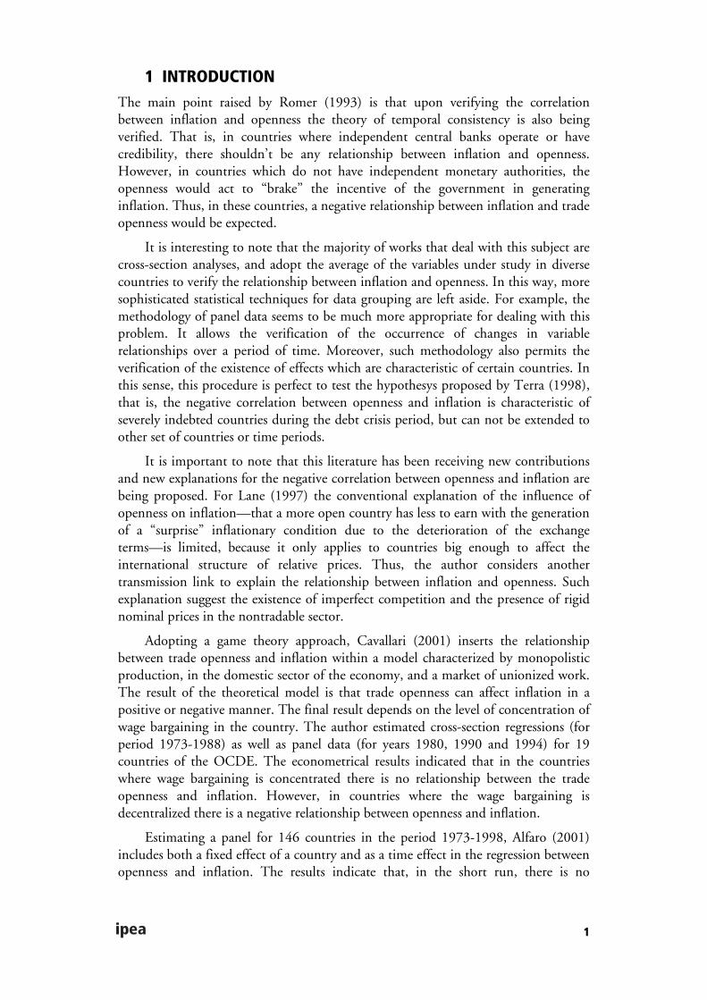
SINOPSENeste artigo é estimada a relação entre inflação e abertura comercial [e.g., Romer(1993)] usando a metodologia de dados em painel. A vantagem desse método é apossibilidade de testar com maior grau de acuidade a hipótese sugerida por Terra(1998) de que a relação negativa entre abertura e inflação se deve à presença, naamostra, de países severamente endividados durante o período da crise da dívidaexterna. Os resultados econométricos dão suporte aos achados de Romer (1993),mostrando que a relação negativa entre abertura comercial e inflação não está restritaa um subconjunto de países e nem a um específico período de tempo.

ABSTRACTIn this article we estimate the relationship between inflation and trade openness [e.g.,Romer (1993)] using modern panel data techniques. The advantage here is that weare able to explicit test the hypothesis proposed by Terra (1998) that the negativerelationship between openness and inflation is due to severely indebted countries inthe debt crisis period. The econometric results give support to Romer (1993)showing that the negative relationship between inflation and openness are neitherrestrict to a subset of countries or a time period.

1

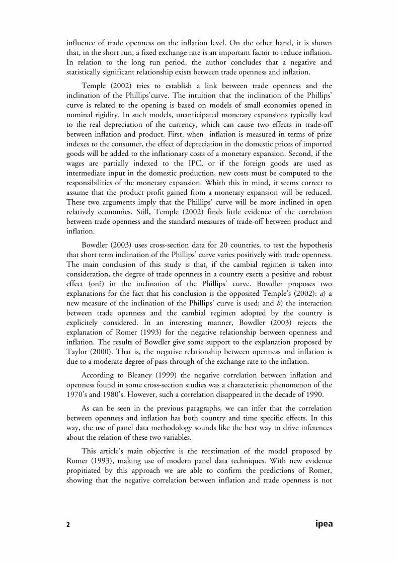
1 INTRODUCTIONThe main point raised by Romer (1993) is that upon verifying the correlationbetween inflation and openness the theory of temporal consistency is also beingverified. That is, in countries where independent central banks operate or havecredibility, there shouldn’t be any relationship between inflation and openness.However, in countries which do not have independent monetary authorities, theopenness would act to “brake” the incentive of the government in generatinginflation. Thus, in these countries, a negative relationship between inflation and tradeopenness would be expected.

It is interesting to note that the majority of works that deal with this subject arecross-section analyses, and adopt the average of the variables under study in diversecountries to verify the relationship between inflation and openness. In this way, moresophisticated statistical techniques for data grouping are left aside. For example, themethodology of panel data seems to be much more appropriate for dealing with thisproblem. It allows the verification of the occurrence of changes in variablerelationships over a period of time. Moreover, such methodology also permits theverification of the existence of effects which are characteristic of certain countries. Inthis sense, this procedure is perfect to test the hypothesys proposed by Terra (1998),that is, the negative correlation between openness and inflation is characteristic ofseverely indebted countries during the debt crisis period, but can not be extended toother set of countries or time periods.

It is important to note that this literature has been receiving new contributionsand new explanations for the negative correlation between openness and inflation arebeing proposed. For Lane (1997) the conventional explanation of the influence ofopenness on inflation—that a more open country has less to earn with the generationof a “surprise” inflationary condition due to the deterioration of the exchangeterms—is limited, because it only applies to countries big enough to affect theinternational structure of relative prices. Thus, the author considers anothertransmission link to explain the relationship between inflation and openness. Suchexplanation suggest the existence of imperfect competition and the presence of rigidnominal prices in the nontradable sector.

Adopting a game theory approach, Cavallari (2001) inserts the relationshipbetween trade openness and inflation within a model characterized by monopolisticproduction, in the domestic sector of the economy, and a market of unionized work.The result of the theoretical model is that trade openness can affect inflation in apositive or negative manner. The final result depends on the level of concentration ofwage bargaining in the country. The author estimated cross-section regressions (forperiod 1973-1988) as well as panel data (for years 1980, 1990 and 1994) for 19countries of the OCDE. The econometrical results indicated that in the countrieswhere wage bargaining is concentrated there is no relationship between the tradeopenness and inflation. However, in countries where the wage bargaining isdecentralized there is a negative relationship between openness and inflation.

Estimating a panel for 146 countries in the period 1973-1998, Alfaro (2001)includes both a fixed effect of a country and as a time effect in the regression betweenopenness and inflation. The results indicate that, in the short run, there is no

2

influence of trade openness on the inflation level. On the other hand, it is shownthat, in the short run, a fixed exchange rate is an important factor to reduce inflation.In relation to the long run period, the author concludes that a negative andstatistically significant relationship exists between trade openness and inflation.

Temple (2002) tries to establish a link between trade openness and theinclination of the Phillips’curve. The intuition that the inclination of the Phillips’curve is related to the opening is based on models of small economies opened innominal rigidity. In such models, unanticipated monetary expansions typically leadto the real depreciation of the currency, which can cause two effects in trade-offbetween inflation and product. First, when inflation is measured in terms of prizeindexes to the consumer, the effect of depreciation in the domestic prices of importedgoods will be added to the inflationary costs of a monetary expansion. Second, if thewages are partially indexed to the IPC, or if the foreign goods are used asintermediate input in the domestic production, new costs must be computed to theresponsibilities of the monetary expansion. Whith this in mind, it seems correct toassume that the product profit gained from a monetary expansion will be reduced.These two arguments imply that the Phillips’ curve will be more inclined in openrelatively economies. Still, Temple (2002) finds little evidence of the correlationbetween trade openness and the standard measures of trade-off between product andinflation.

Bowdler (2003) uses cross-section data for 20 countries, to test the hypothesisthat short term inclination of the Phillips’ curve varies positively with trade openness.The main conclusion of this study is that, if the cambial regimen is taken intoconsideration, the degree of trade openness in a country exerts a positive and robusteffect (on?) in the inclination of the Phillips’ curve. Bowdler proposes twoexplanations for the fact that his conclusion is the opposited Temple’s (2002): a) anew measure of the inclination of the Phillips’ curve is used; and b) the interactionbetween trade openness and the cambial regimen adopted by the country isexplicitely considered. In an interesting manner, Bowdler (2003) rejects theexplanation of Romer (1993) for the negative relationship between openness andinflation. The results of Bowdler give some support to the explanation proposed byTaylor (2000). That is, the negative relationship between openness and inflation isdue to a moderate degree of pass-through of the exchange rate to the inflation.

According to Bleaney (1999) the negative correlation between inflation andopenness found in some cross-section studies was a characteristic phenomenon of the1970’s and 1980’s. However, such a correlation disappeared in the decade of 1990.

As can be seen in the previous paragraphs, we can infer that the correlationbetween openness and inflation has both country and time specific effects. In thisway, the use of panel data methodology sounds like the best way to drive inferencesabout the relation of these two variables.

This article’s main objective is the reestimation of the model proposed byRomer (1993), making use of modern panel data techniques. With new evidencepropitiated by this approach we are able to confirm the predictions of Romer,showing that the negative correlation between inflation and trade openness is not

3

restricted to a subset of countries nor a time period. In the next section we describethe dataset and the econometric results. Section 3 concludes the article.

2 ECONOMETRIC RESULTSThe data used in this study were obtained from Summers and Heston (1988), andconsist of a total of 152 countries in the period of 1950-1992.1 Such as in Romer(1993), the following model was estimated:

Log of inflationit = αι + βι opennessit (1)

Where subscript i represents country i and t the time. Moreover α is theconstant (subscript ι indicates that it can be different for each group of countries) andβ is the inclination coefficient (again, it is allowed that this parameter be distinct foreach group of countries). Log of the inflation is the natural logarithm of change inthe implicit deflator of the GDP. The degree of openness is measured as the rate ofthe importations in relation to the GDP. The countries have been grouped in 7distinct groups, in the following way: Group 1: Africa; Group 2: North and CentralAmerica; Group 3: South America; Group 4: Asia; Group 5: Europe; Group 6:Oceania; and Group 7: countries pertaining to the OCDE.2

In the present work, the estimate between trade openness and inflation bymodels of panel data are the great advantage in relation to estimates by cross-sectionor time series because it makes test hypothesis on specific groups of countriespossible. Thus we can explicitly test the idea proposed by Terra (1998) stating thatthe negative relationship between inflation and openness can only be verified in thedebt crisis period of 1982-1990 in severely indebted countries.

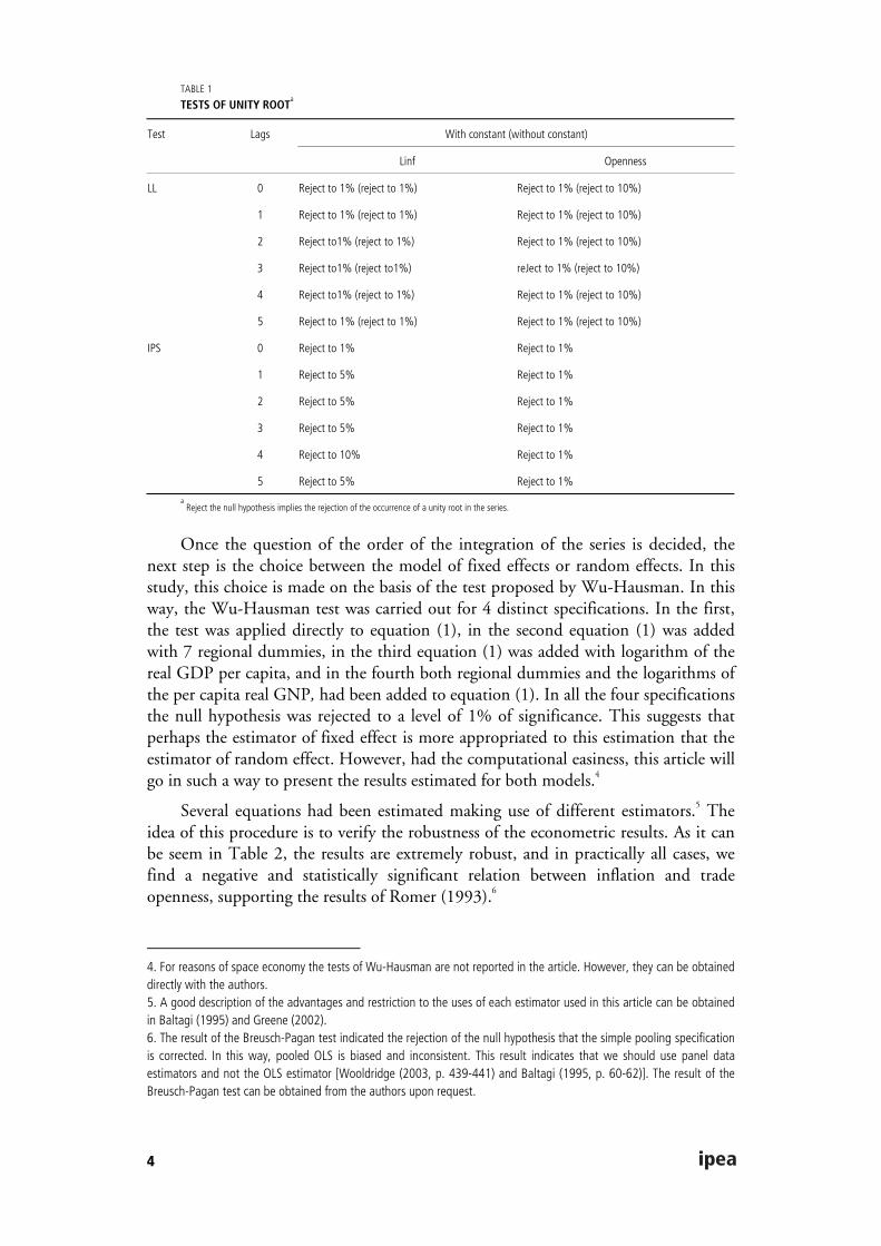
To verify the order of integration of the series, the tests of unitary root proposedby Levin, Lin and Chu (2002) and Im, Pesaran and Shin (2003) were carried out.Moreover, such tests were carried out for different numbers of lags and differentdeterministic components.3 As a set, the results were shown to be robust in rejectingthe null hypothesis of unity root in the series of logarithm of inflation (Linf) andtrade openness. As one can observe in Table 1, the tests of Levin, Lin and Chu (LLC)and Im, Pesaran and Smith (IPS) always reject the null hypothesis of unity root to alevel of at least 10% of statistical significance. We may then conclude that bothvariables are integrated of order zero (I(0)).

1. They can be accessed on the Internet at the address <http://pwt.econ.upenn.edu>.2. The countries belonging to OCDE were taken from their group of geographical location. Thus, for example, the UnitedStates belongs to Group 7 (OCDE) and not to Group 2 (North and Central America).3. This procedure is important, because just as in the tests of unitary root for temporary series, the choice of the numberof lags and of the deterministic components can alter the result of the test.

4

TABLE 1

TESTS OF UNITY ROOTa

Test Lags With constant (without constant)

Linf Openness

LL 0 Reject to 1% (reject to 1%) Reject to 1% (reject to 10%)

1 Reject to 1% (reject to 1%) Reject to 1% (reject to 10%)

2 Reject to1% (reject to 1%) Reject to 1% (reject to 10%)

3 Reject to1% (reject to1%) reJect to 1% (reject to 10%)

4 Reject to1% (reject to 1%) Reject to 1% (reject to 10%)

5 Reject to 1% (reject to 1%) Reject to 1% (reject to 10%)

IPS 0 Reject to 1% Reject to 1%

1 Reject to 5% Reject to 1%





a Reject the null hypothesis implies the rejection of the occurrence of a unity root in the series.

Once the question of the order of the integration of the series is decided, thenext step is the choice between the model of fixed effects or random effects. In thisstudy, this choice is made on the basis of the test proposed by Wu-Hausman. In thisway, the Wu-Hausman test was carried out for 4 distinct specifications. In the first,the test was applied directly to equation (1), in the second equation (1) was addedwith 7 regional dummies, in the third equation (1) was added with logarithm of thereal GDP per capita, and in the fourth both regional dummies and the logarithms ofthe per capita real GNP, had been added to equation (1). In all the four specificationsthe null hypothesis was rejected to a level of 1% of significance. This suggests thatperhaps the estimator of fixed effect is more appropriated to this estimation that theestimator of random effect. However, had the computational easiness, this article willgo in such a way to present the results estimated for both models.4

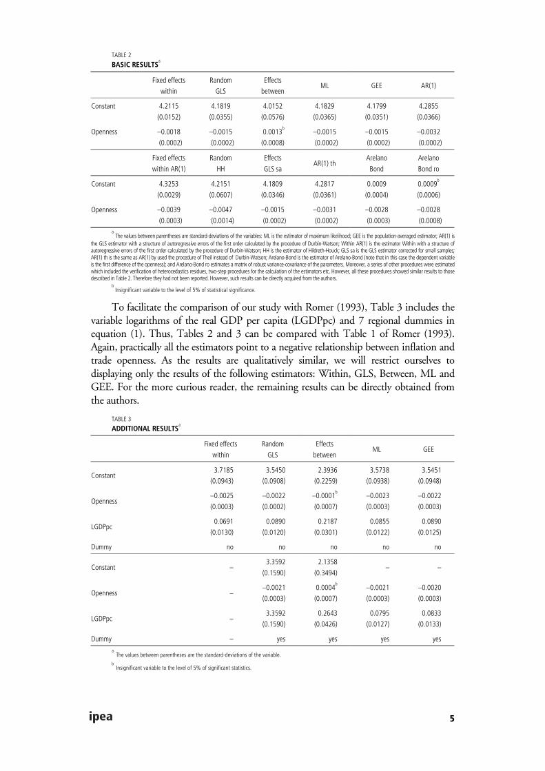
Several equations had been estimated making use of different estimators.5 Theidea of this procedure is to verify the robustness of the econometric results. As it canbe seem in Table 2, the results are extremely robust, and in practically all cases, wefind a negative and statistically significant relation between inflation and tradeopenness, supporting the results of Romer (1993).6

4. For reasons of space economy the tests of Wu-Hausman are not reported in the article. However, they can be obtaineddirectly with the authors.5. A good description of the advantages and restriction to the uses of each estimator used in this article can be obtainedin Baltagi (1995) and Greene (2002).6. The result of the Breusch-Pagan test indicated the rejection of the null hypothesis that the simple pooling specificationis corrected. In this way, pooled OLS is biased and inconsistent. This result indicates that we should use panel dataestimators and not the OLS estimator [Wooldridge (2003, p. 439-441) and Baltagi (1995, p. 60-62)]. The result of theBreusch-Pagan test can be obtained from the authors upon request.

5

TABLE 2

BASIC RESULTSa

Fixed effects

within

Random

GLS

Effects

betweenML GEE AR(1)

Constant 4.2115

(0.0152)

4.1819

(0.0355)

4.0152

(0.0576)

4.1829

(0.0365)

4.1799

(0.0351)

4.2855

(0.0366)

Openness –0.0018

(0.0002)

–0.0015

(0.0002)

0.0013b

(0.0008)

–0.0015

(0.0002)

–0.0015

(0.0002)

–0.0032

(0.0002)

Fixed effects

within AR(1)

Random

HH

Effects

GLS saAR(1) th

Arelano

Bond

Arelano

Bond ro

Constant 4.3253

(0.0029)

4.2151

(0.0607)

4.1809

(0.0346)

4.2817

(0.0361)

0.0009

(0.0004)

0.0009b

(0.0006)

Openness –0.0039

(0.0003)

–0.0047

(0.0014)

–0.0015

(0.0002)

–0.0031

(0.0002)

–0.0028

(0.0003)

–0.0028

(0.0008)a The values between parentheses are standard-deviations of the variables: ML is the estimator of maximum likelihood; GEE is the population-averaged estimator; AR(1) is

the GLS estimator with a structure of autoregressive errors of the first order calculated by the procedure of Durbin-Watson; Within AR(1) is the estimator Within with a structure ofautoregressive errors of the first order calculated by the procedure of Durbin-Watson; HH is the estimator of Hildreth-Houck; GLS sa is the GLS estimator corrected for small samples;AR(1) th is the same as AR(1) by used the procedure of Theil instead of Durbin-Watson; Arelano-Bond is the estimator of Arelano-Bond (note that in this case the dependent variableis the first difference of the openness); and Arelano-Bond ro estimates a matrix of robust variance-covariance of the parameters. Moreover, a series of other procedures were estimatedwhich included the verification of heterocedastics residues, two-step procedures for the calculation of the estimators etc. However, all these procedures showed similar results to thosedescribed in Table 2. Therefore they had not been reported. However, such results can be directly acquired from the authors.

b Insignificant variable to the level of 5% of statistical significance.

To facilitate the comparison of our study with Romer (1993), Table 3 includes thevariable logarithms of the real GDP per capita (LGDPpc) and 7 regional dummies inequation (1). Thus, Tables 2 and 3 can be compared with Table 1 of Romer (1993).Again, practically all the estimators point to a negative relationship between inflation andtrade openness. As the results are qualitatively similar, we will restrict ourselves todisplaying only the results of the following estimators: Within, GLS, Between, ML andGEE. For the more curious reader, the remaining results can be directly obtained fromthe authors.

TABLE 3

ADDITIONAL RESULTSa

Fixed effects

within

Random

GLS

Effects

betweenML GEE

Constant3.7185

(0.0943)

3.5450

(0.0908)

2.3936

(0.2259)

3.5738

(0.0938)

3.5451

(0.0948)

Openness–0.0025

(0.0003)

–0.0022

(0.0002)

–0.0001b

(0.0007)

–0.0023

(0.0003)

–0.0022

(0.0003)

LGDPpc0.0691

(0.0130)

0.0890

(0.0120)

0.2187

(0.0301)

0.0855

(0.0122)

0.0890

(0.0125)

Dummy no no no no no

Constant –3.3592

(0.1590)

2.1358

(0.3494)– –

Openness ––0.0021

(0.0003)

0.0004b

(0.0007)

–0.0021

(0.0003)

–0.0020

(0.0003)

LGDPpc –3.3592

(0.1590)

0.2643

(0.0426)

0.0795

(0.0127)

0.0833

(0.0133)

Dummy – yes yes yes yes

aThe values between parentheses are the standard-deviations of the variable.

bInsignificant variable to the level of 5% of significant statistics.

6

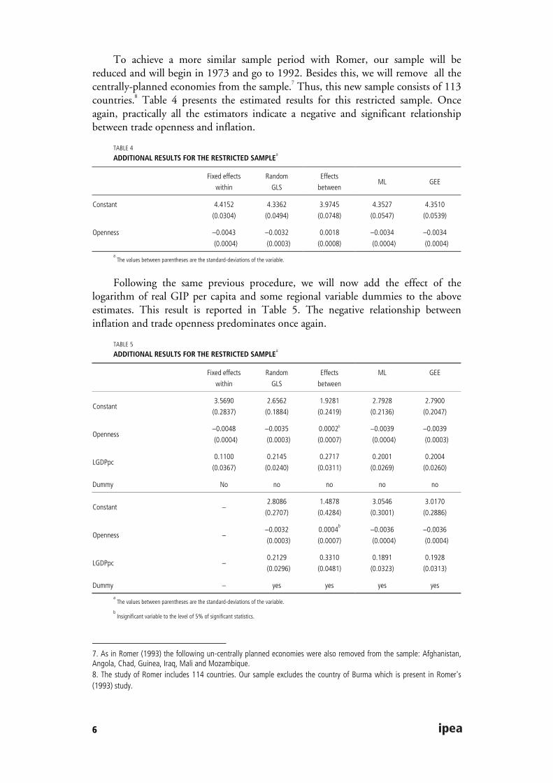
To achieve a more similar sample period with Romer, our sample will bereduced and will begin in 1973 and go to 1992. Besides this, we will remove all thecentrally-planned economies from the sample.7 Thus, this new sample consists of 113countries.8 Table 4 presents the estimated results for this restricted sample. Onceagain, practically all the estimators indicate a negative and significant relationshipbetween trade openness and inflation.

TABLE 4

ADDITIONAL RESULTS FOR THE RESTRICTED SAMPLEa

Fixed effects

within

Random

GLS

Effects

betweenML GEE

Constant 4.4152

(0.0304)

4.3362

(0.0494)

3.9745

(0.0748)

4.3527

(0.0547)

4.3510

(0.0539)

Openness –0.0043

(0.0004)

–0.0032

(0.0003)

0.0018

(0.0008)

–0.0034

(0.0004)

–0.0034

(0.0004)

a The values between parentheses are the standard-deviations of the variable.

Following the same previous procedure, we will now add the effect of thelogarithm of real GIP per capita and some regional variable dummies to the aboveestimates. This result is reported in Table 5. The negative relationship betweeninflation and trade openness predominates once again.

TABLE 5

ADDITIONAL RESULTS FOR THE RESTRICTED SAMPLEa

Fixed effects

within

Random

GLS

Effects

between

ML GEE

Constant3.5690

(0.2837)

2.6562

(0.1884)

1.9281

(0.2419)

2.7928

(0.2136)

2.7900

(0.2047)

Openness–0.0048

(0.0004)

–0.0035

(0.0003)

0.0002b

(0.0007)

–0.0039

(0.0004)

–0.0039

(0.0003)

LGDPpc0.1100

(0.0367)

0.2145

(0.0240)

0.2717

(0.0311)

0.2001

(0.0269)

0.2004

(0.0260)

Dummy No no no no no

Constant –2.8086

(0.2707)

1.4878

(0.4284)

3.0546

(0.3001)

3.0170

(0.2886)

Openness ––0.0032

(0.0003)

0.0004b

(0.0007)

–0.0036

(0.0004)

–0.0036

(0.0004)

LGDPpc –0.2129

(0.0296)

0.3310

(0.0481)

0.1891

(0.0323)

0.1928

(0.0313)

Dummy – yes yes yes yes

a The values between parentheses are the standard-deviations of the variable.

b Insignificant variable to the level of 5% of significant statistics.

7. As in Romer (1993) the following un-centrally planned economies were also removed from the sample: Afghanistan,Angola, Chad, Guinea, Iraq, Mali and Mozambique.8. The study of Romer includes 114 countries. Our sample excludes the country of Burma which is present in Romer's(1993) study.

7

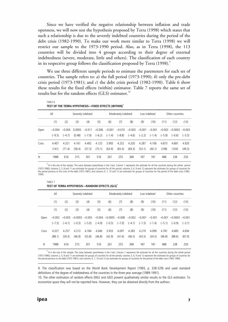
Since we have verified the negative relationship between inflation and tradeopenness, we will now test the hypothesis proposed by Terra (1998) which states thatsuch a relationship is due to the severely indebted countries during the period of thedebt crisis (1982-1990). To make our work more similar to Terra (1998) we willrestrict our sample to the 1973-1990 period. Also, as in Terra (1998), the 113countries will be divided into 4 groups according to their degree of externalindebtedness (severe, moderate, little and others). The classification of each countryin its respective group follows the classification proposed by Terra (1998).9

We use three different sample periods to estimate the paremeters for each set ofcountries. The sample refers to: a) the full period (1973-1990); b) only the pre-debtcrisis period (1973-1981); and c) the debt crisis period (1982-1990). Table 6 showthese results for the fixed effects (within) estimator. Table 7 reports the same set ofresults but for the random effects (GLS) estimator.10

TABLE 6

TEST OF THE TERRA HYPOTHESIS—FIXED EFFECTS (WITHIN)a

All Severely indebted Moderately indebted Low indebted Other countries

(1) (2) (3) (4) (5) (6) (7) (8) (9) (10) (11) (12) (13)

Open –0.004

(–9.5)

–0.004

(–4.7)

0.0005

(0.48)

–0.011

(–7.9)

–0.006

(–6.2)

–0.001

(–1.4)

–0.010

(–8.8)

–0.003

(–4.6)

–0.001

(–2.2)

–0.001

(–1.4)

–0.003

(–5.9)

–0.0003

(–0.6)

–0.003

(–3.5)

Cons 4.407

(141)

4.321

(71.4)

4.161

(58.4)

4.492

(57.3)

4.125

(75.1)

3.993

(63.9)

4.232

(65.4)

4.320

(69.3)

4.287

(53.1)

4.106

(40.1)

4.873

(108)

4.681

(104)

4.920

(49.3)

N 1988 616 315 301 516 261 255 368 187 181 488 238 250

a N is the size of the sample. The value between parentheses is the t-test. Column 1 represents the estimate for all the countries during the whole period

(1973-1990); columns 2, 5, 8 and 11 are estimates for groups of countries for all the period; columns 3, 6, 9 and 12 represent the estimates for groups of countries forthe period previous to the crisis of the debt (1973-1981); and columns 4, 7, 10 and 13 are estimates for groups of countries for the period of the debt crisis (1982-1990).

TABLE 7

TEST OF TERRA HYPOTHESIS—RANDOM EFFECTS (GLS)a


(1) (2) (3) (4) (5) (6) (7) (8) (9) (10) (11) (12) (13)

(1) (2) (3) (4) (5) (6) (7) (8) (9) (10) (11) (12) (13)

Open –0.002

(–7.5)

–0.003

(–4.1)

–0.0003

(–0.3)

–0.005

(–5.0)

–0.004

(–4.9)

–0.0005

(–0.5)

–0.008

(–7.0)

–0.002

(–4.1)

–0.001

(–1.5)

–0.001

(–1.4)

–0.001

(–5.1)

–0.0003

(–0.9)

–0.001

(–3.1)

Cons 4.327

(88.1)

4.257

(59.3)

4.213

(46.9)

4.184

(55.8)

4.040

(46.8)

3.933

(42.9)

4.097

(41.6)

4.283

(46.5)

4.219

(43.5)

4.099

(34.5)

4.781

(96.8)

4.685

(88.6)

4.694

(87.0)

N 1988 616 315 301 516 261 255 368 187 181 488 238 250


(1973-1990); columns 2, 5, 8 and 11 are estimates for groups of countries for all the period; columns 3, 6, 9 and 12 represent the estimates for groups of countries forthe period previous to the debt (1973-1981); and columns 4, 7, 10 and 13 are estimates for groups of countries for the period of the debt crisis (1982-1990).

9. The classification was based on the World Bank Development Report (1993, p. 328-329) and used standarddefinitions of the degree of indebtedness of the countries in the three year average (1989-1991).10. The other estimators of random effects (MLE and GEE) present qualitatively similar results to the GLS estimator. Toeconomize space they will not be reported here. However, they can be obtained directly from the authors.

8

In relation to the 13 regressions which appear both in Table 6 and 7, we mustremember that: a) column 1 represents the estimate for all the countries during allthe period (1973-1990); b) columns 2, 5, 8 and 11 are estimates for groups ofcountries for all the period; c) columns 3, 6, 9 and 12 represent the estimates forgroups of countries for the period previous to the debt crisis (1973-1981); and d)columns 4, 7, 10 and 13 are estimates for groups of countries for the period of thedebt crisis (1982-1990). With this, the test of the hypothesis proposed by Terra(1998) can be carried out by a simple t-test over the coefficient of openness incolumns 3, 4, 6, 7, 9, 10, 12 and 13. In accordance with Terra (1998) the negativerelationship between openness and inflation occurs only in the severely indebtedcountries, during the period of the debt crisis. Thus, in agreement with Terra (1998)the coefficient of openness should be negative and statistically significant only incolumn 4, being statistically insignificant in columns 3, 6, 7, 9, 10, 12 and 13.

Observing Table 6, we notice that the coefficients of openness are insignificant,at 5% of statistical significance, for columns 3, 6, 10 and 12, being significant andnegative for column 4. Thus, the Terra hypothesis fails in explaining the behaviorpresent in columns 7, 9 and 13. In relation to Table 7, the openness coefficients areinsignificant in columns 3, 6, 9, 10 and 12, and significant and negative in column 4.With this, the Terra hypothesis fails to explain the behavior in columns 7 and 13.

The test of Wu-Hausman for the choice the model of fixed effects or the modelof random effects was carried out for the 13 estimates present in Tables 6 and 7.Adopting a critical level of 5% of statistical significance, the Wu-Hausman testsuggests the adoption of random effects for the models: 3, 9, 10 and 12. For theremaining models, Wu-Hausman test suggests the adoption of fixed effects.11 Thus,we have that the negative relationship between inflation and openness must berejected for models 3, 6, 9, 10 and 12. This indicates that the negative relationshipbetween inflation and openness only occurs during the period of the debt crisis(1982-1990) and for the following group of countries: severely indebted, moderatelyindebted, and for the other countries. Notice that such results refutes the Terrahypothesis (1998) because, for the author, the negative relationship betweenopenness and inflation must only occur in the severely indebted countries during thedebt crisis.

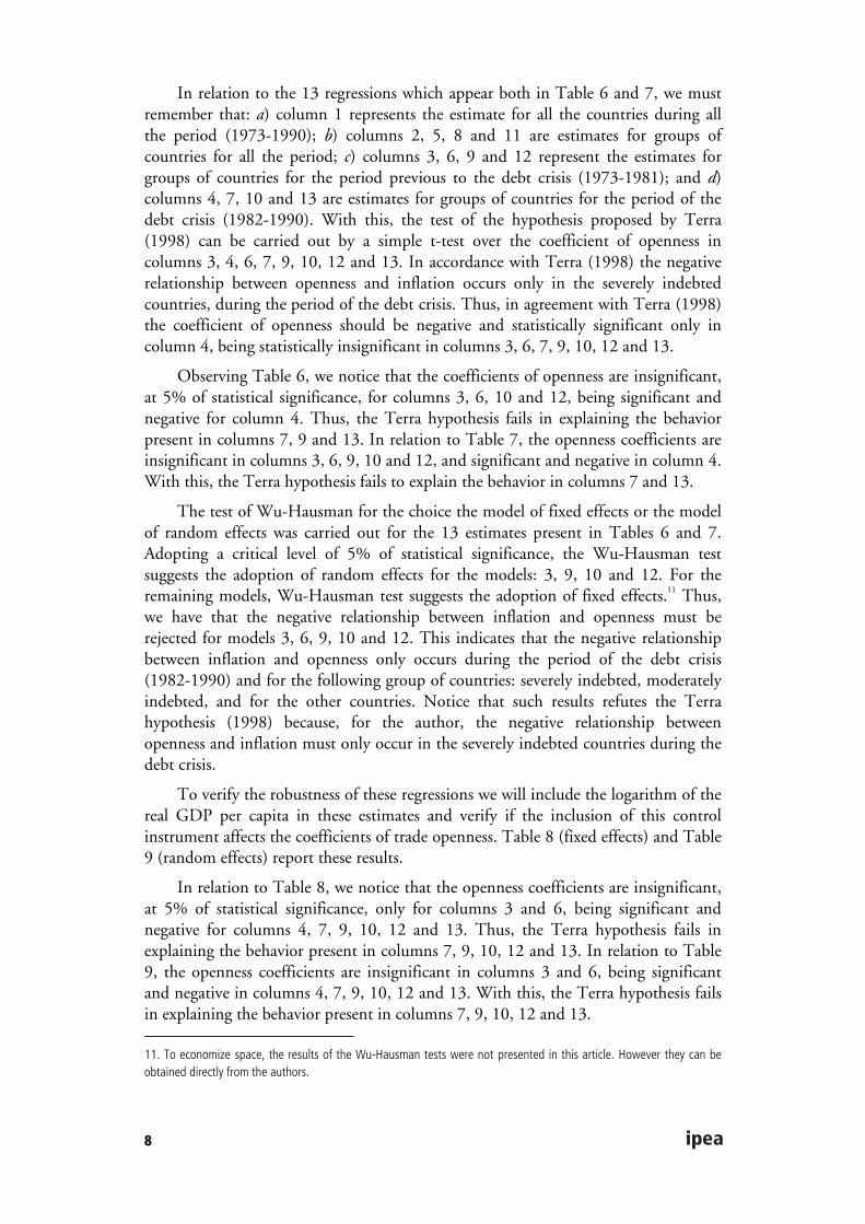
To verify the robustness of these regressions we will include the logarithm of thereal GDP per capita in these estimates and verify if the inclusion of this controlinstrument affects the coefficients of trade openness. Table 8 (fixed effects) and Table9 (random effects) report these results.

In relation to Table 8, we notice that the openness coefficients are insignificant,at 5% of statistical significance, only for columns 3 and 6, being significant andnegative for columns 4, 7, 9, 10, 12 and 13. Thus, the Terra hypothesis fails inexplaining the behavior present in columns 7, 9, 10, 12 and 13. In relation to Table9, the openness coefficients are insignificant in columns 3 and 6, being significantand negative in columns 4, 7, 9, 10, 12 and 13. With this, the Terra hypothesis failsin explaining the behavior present in columns 7, 9, 10, 12 and 13.

11. To economize space, the results of the Wu-Hausman tests were not presented in this article. However they can beobtained directly from the authors.

9

TABLE 8

NEW RESULTS—FIXED EFFECTS (WITHIN)a


(1) (2) (3) (4) (5) (6) (7) (8) (9) (10) (11) (12) (13)

Open –0.004

(–9.7)

–0.005

(–5.4)

0.0008

(0.75)

–0.011

(–8.2)

–0.005

(–5.4)

–0.002

(–1.8)

–0.009

(–8.2)

–0.003

(–4.7)

–0.003

(–3.1)

–0.003

(–3.2)

–0.003

(–6.5)

–0.001

(–3.3)

–0.005

(–6.3)

Lgdp 0.081

(2.1)

0.373

(3.7)

–0.121

(–1.1)

0.558

(3.04)

–0.414

(–5.7)

0.152

(1.4)

–0.511

(–3.9)

0.072

(1.2)

0.165

(2.3)

0.599

(5.5)

0.118

(2.6)

0.439

(5.4)

0.932

(10.3)

Cons 3.776

(12.7)

1.639

(2.2)

5.02

(6.5)

0.444

(0.3)

7.147

(13.5)

2.896

(3.7)

7.994

(8.2)

3.773

(8.5)

3.056

(5.7)

–0.586

(–0.6)

3.825

(9.5)

0.795

(1.1)

–3.64

(–4.3)

N 1988 616 315 301 516 261 255 368 187 181 488 238 250


(1973-1990); columns 2, 5, 8 and 11 are estimates for groups of countries for all the period; columns 3, 6, 9 and 12 represent the estimates for groups of countries forthe period previous to the debt crisis (1973-1981); and columns 4, 7, 10 and 13 are estimates for groups of countries for the period of the debt crisis (1982-1990).

TABLE 9

NEW RESULTS—RANDOM EFFECTS (GLS)a


(1) (2) (3) (4) (5) (6) (7) (8) (9) (10) (11) (12) (13)

Open –0.003

(–8.5)

–0.003

(–4.4)

–0.000

(–0.0)

–0.005

(–5.2)

–0.004

(–4.3)

–0.0006

(–0.6)

–0.007

(–6.7)

–0.003

(–4.7)

–0.002

(–2.8)

–0.002

(–3.3)

–0.001

(–5.2)

–0.0007

(–2.0)

–0.001

(–3.0)

Lgdp 0.202

(8.2)

0.108

(1.86)

–0.096

(–1.3)

0.098

(1.6)

–0.116

(–2.0)

0.248

(3.9)

–0.060

(–0.7)

0.134

(2.8)

0.174

(3.2)

0.424

(6.3)

0.103

(2.6)

0.321

(5.8)

0.655

(9.0)

Cons 2.741

(14.2)

3.486

(8.2)

4.900

(9.6)

3.485

(8.1)

4.864

(11.4)

2.108

(4.5)

4.532

(7.1)

3.246

(8.7)

2.920

(7.1)

0.783

(1.4)

3.805

(10.5)

1.760

(3.4)

–1.47

(–2.1)

N 1988 616 315 301 516 261 255 368 187 181 488 238 250


(1973-1990); columns 2, 5, 8 and 11 are estimates for groups of countries for all the period; columns 3, 6, 9 and 12 represent the estimates for groups of countries forthe period previous to the debt crisis (1973-1981); and columns 4, 7, 10 and 13 are estimates for groups of countries for the period of the debt crisis (1982-1990).

The test of Wu-Hausman for the choice between the model of fixed effects orthe model of random effects was carried out for the 13 estimates present in Tables 8and 9. Adopting a critical level of 5% of statistical significance, the Wu-Hausmantest suggests the adoption of random effects for the models: 3, 9 and 10. For theremaining models, the test suggests the adoption of fixed effects.12 Thus, we have thatthe negative relationship between inflation and openness must be rejected only formodels 3 and 6. This indicates that the negative relationship between inflation andopenness occurs in severely indebted countries and in the rest of the countries, duringthe period of the debt crisis and in the period previous to the debt crisis. Again, thisresult refutes the Terra hypothesis.

12. Seeking the space economy, the results of the tests of Wu-Hausman were not showed in this article. However theycan be obtained directly with the authors.

10

3 CONCLUSIONThe main objective of this article was to apply the panel data methodology to verifythe hypothesis proposed by Romer (1993), which states a negative relationshipbetween trade openness and inflation. The econometric results corroborates Romer’sfindings, showing great robustness to both different specifications and different timeperiods.

The hypothesis developed by Terra (1998), stating that the negative relationshipbetween inflation and openness was due to severely indebted countries, during thedebt crisis, was explicitly tested and rejected. It was shown that the negativerelationship between inflation and openness occurs not just in the severely indebtedcountries, but in other groups of countries too, during the debt crisis period as well asin the period previous to the debt crisis.

In a summarized way, this study strengthens the results which Romer (1993 and1998) presented, showing that a negative relationship between openness and inflationexists. Moreover, it was showed that such a relationship is not specific to any groupof countries nor specific to a determined period of time. Thus, countries thatexperienced an increase of openness also observed a reduction in their levels ofinflation.

BIBLIOGRAPHYALFARO, L. Inflation, openness and exchange rate regimes: The Quest for Short-Term

Commitment. Harvard Business School, 2001 (Working Paper Series, 02-014).

ASHRA, S. Inflation and openness: a study of selected development economies. Indian CouncilFor Research on International Economic Relations. May 2002 (Working Paper, 84).

BALTAGI, B. H. Econometric analysis of panel data. John Wiley & Sons, 1995.

BARRO, R. J., GORDON, D. B. A positive theory of monetary policy in a natural ratemodel. Journal of Political Economy, v. 91, n. 4, p. 589-610, 1983.

BILGINSOY, C. Inflation, growth, and import bottlenecks in the turkish manufacturingindustry. Journal of Developments Economics, v. 42, p. 111-31, 1993.

BLEANEY, M. The disappearing openness-inflation relationship: a cross-country analysis ofinflation rates. IMF, Dec. 1999 (Working Paper, 161).

BOWDLER, C. Openness and output-inflation tradeoff. Nuffield College, Mar. 2003(Working Paper).

CAVALLARI, L. Inflation and openness with non-atomistic wage setters. University of Rome“La Sapienza”, 2001 (Working Paper).

DIELMAN, T. E. Pooled cross-section and time series data analysis. New York: Marcel Dekker,1989.

DEATON, A. Panel data from a series of repeated cross-sections. Journal of Econometrics,v. 30, p. 109-126, 1985.

ENDERS, W. Applied econometric time series. New York: John Wiley and Sons, 1995.

11

GRANGER, C., NEWBOLD, P. Spurious regressions in econometrics. Journal ofEconometrics, v. 2, p. 111-120, 1974.

GREENE, W. H. Econometric Analysis. 5th ed. Prentice Hall, 2002.

HARDOUVELIS, G. A. Monetary policy games, inflationary bias, and openness. Journal ofEconomic Dynamics and Control, v. 16, p. 147-164, Jan. 1992.

HSIAO, C. Analysis of panel data. Econometric Society Monographs, n. 11, 1986.

IM, K. S., PESARAN, M. H., SHIN, Y. Testing for unit roots in heterogeneous panels.Journal of Econometrics, v. 115, p. 53-74, 2003.

JIN, J. C. Openness, growth and inflation: evidence from South Korea. Chinese University ofHong Kong, 2000 (Working Paper).

JOHNSTON, J., DINARDO, J. Econometric Methods. 4th ed. McGraw-Hill, 1997.

KENNEDY, P. A guide to econometrics. 4th ed. Cambridge, Massachusetts: MIT Press, 1998.

KYDLAND, F. E., PRESCOTT, E. C. Rules rather than discretion: the inconsistency ofoptimal plans. Journal of Political Economy, v. 85, n. 3, p. 473-491, June 1977.

LANE, P. R. Inflation in open economics. Journal of International Economics, v. 42, p. 327-347, 1997.

LEVIN, A., LIN, C.-F., JAMES CHU, C.-S. Unit root tests in panel data: asymptotic andfinite-sample properties. Journal of Econometrics, Elsevier, v. 108, n. 1, p. 1-24, 2002.

LO, M., WONG, M. C. S., GRANATO, J. Openness and aggressive monetary policy: a studyof inflation volatility and persistence. University of Southern Mississippi, 2003 (WorkingPaper).

MADDALA, G. S., KIM, I-M. Unit roots, cointegration, and structural change. CambridgeUniversity Press, 2000.

MATYAS, L., SEVESTRE, P. (eds.) The econometrics of panel data: handbook of theory andapplications. 2nd ed. Dordrecht: Kluwer-Nijoff, 1996.

MOULTON, B. R. Random group effects and the precision of regression estimates. Journalof Econometrics, v. 32, p. 385-397, 1986.

RAJ, B., BALTAGI, B. (eds.) Panel data analysis. Heidelberg: Physica-Verlag, 1992.

ROGOFF, K. Can international monetary policy cooperation be counterproductive? Journalof International Economics, v. 18, p. 199-217, May 1985.

ROMER, D. Openness and inflation: theory and evidence. Quarterly Journal of Economics,v. 108, n. 4, p. 869-903, Nov. 1993.

—————. A new assessment of openness and inflation: reply. Quarterly Journal ofEconomics, p. 649-52, May 1998.

SUMMERS, R., HESTON, A. A new set of international comparisons of real product andprice levels estimates for 130 countries, 1950-1985. Review of Income and Wealth, v. 34,p. 1-25, Mar. 1988.

TAYLOR, J. B. Low inflation, pass-thought, and the pricing power of firms. EuropeanEconomic Review, Elsevier, v. 44, n. 7, p. 1.389-1.408, 2000.

12

TELLA, R., MacCULLOCH, R. Unemployment benefits as a substitute for a conservativecentral banker. Harvard Business School, May 2000 (Working Paper Series).

TEMPLE, J. Openness, inflation and the Phillips Curve: a puzzle. Journal of Money, Creditand Banking, 2002 (forthcoming).

TERRA, C. T. Debt crisis and inflation. Revista de Econometria, v. 17, p. 21-48, Nov. 1997.

TERRA, C. T. Openness and inflation: a new assessment. Quarterly Journal of Economics, p.641-648, May 1998.

WALSH, C. E. Monetary theory and policy. Massachusetts Institute of Technology, 1998.

WOOLDRIDGE, L. M. Introductory econometrics. 2nd ed. South-Western, 2003

Ipea – Institute for Applied Economic Research

PUBLISHING DEPARTMENT

CoordinationCláudio Passos de Oliveira

SupervisionEverson da Silva MouraReginaldo da Silva Domingos

TypesettingBernar José VieiraCristiano Ferreira de AraújoDaniella Silva NogueiraDanilo Leite de Macedo TavaresDiego André Souza SantosJeovah Herculano Szervinsk JuniorLeonardo Hideki Higa

Cover designLuís Cláudio Cardoso da Silva

Graphic designRenato Rodrigues Buenos

The manuscripts in languages other than Portuguese published herein have not been proofread.

Ipea Bookstore

SBS – Quadra 1 − Bloco J − Ed. BNDES, Térreo 70076-900 − Brasília – DFBrazilTel.: + 55 (61) 3315 5336E-mail: [email protected]

Composed in Adobe Garamond 11/13.2 (text)Frutiger 47 (headings, graphs and tables)

Brasília – DF – Brazil

Ipea’s missionEnhance public policies that are essential to Brazilian development by producing and disseminating knowledge and by advising the state in its strategic decisions.

INFLATION AND TRADE OPENNESS REVISED: AN...

Documents

Transcript of INFLATION AND TRADE OPENNESS REVISED: AN...