Infinite Groups - Jyväskylän yliopistousers.jyu.fi/~laurikah/REP/REPtext2010_4E.pdf · Infinite...

GROUPS AND THEIR REPRESENTATIONS - FOURTHPILE, ALMOST IN ENGLISH

KAREN E. SMITH

22. Infinite Groups

Example 22.1. Many, in fact most well known and important groupsare infinite:

(1) The group of translations (Rn,+)(2) The group of invertible linear mappings GL(Rn) ∼ GLn(R) ={invertible n× n−matrices} with matrix multiplication.

(3) The group of volume and orientation preserving invertible li-near mappings SL(Rn) ∼ SLn(R) = {n × n−matrices withdeterminant 1}.

(4) The group of length, angle and orientation preserving inver-tible linear mappings also called orhtogonaal linear mappingsO(Rn) ∼ SOn(R) = {n× n−matrices with orthogonal columnsor, equivalently, rows and determinant 1} SO(Rn) ∼ SOn(R)

(5) The Lorentz group SO3,1(R), of invertible linear mappings pre-serving a given Minkowski product.

(6) The group of complex invertible linear mappings GL(Cn) ∼ GLn(R) ={invertible complex n× n−matrices}.

(7) The group of unitary linear mappings U(Cn) ∼ Un(C) = {complexn× n−matrices preserving a Hermitian inner product}={ n×n−matrices with orthogonal columns or, equivalently, rows}

(8) SU(Cn) ∼ SUn(C) = {orientation preserving mappings in U(Cn)(9) A special case: U(C) = U(1) = {λ ∈ C

∣∣ |λ| = 1} ∼{rotationsin the plane}.

(10) Products and many factor groups of the afore mentioned.

Remark 22.2. All these act by definition in sope set, most act linearlyin a finite dimensional vector space, so they have tautological represen-tations. It is a nontrivial task to find (all) other representations. Wewill find some. It is not quite evident how one could generalize thetheory of finite groups, as the infinite groups are very large, all of the

1

2 KAREN E. SMITH

above are uncountable and most even lacking countable sets of gene-rators. (Cf. ??, where generators of GLn(R) are given). Fortunately,these groups carry other structure beside the group multiplication, allare topological spaces, and even better, smooth manifolds. Their groupoperations are smooth as well. Such groups are called Lie groups

23. Smooth manifolds and Lie groups

Remark 23.1. INTRODUCTION: (((( Jo aluksi voi hahmotella, mistais kysymys. manifold is tavallisen smoothn pinnan yleistys, yleensa mo-niulotteinen — siita nimi. manifold is siis joukko, usein jonkin korkeau-lotteisen euklideisen avaruuden Rn:n subset, jonka jokaisessa pisteessais olemassa tangenttiavaruus, tangenttitason luonnollinen yleistys. Mo-nistolla is sileita kayria and muita sileita alimonistoja seka ennen kaik-kea monistolta is sileita funktioita luvuille eli koordinaatteja seka sileitakuvauksia muille monistoille and itselleen. Monistolla voi siten harras-taa differentiaalilaskentaa ja, jos se is samalla mitta-avaruus, myos in-tegraalilaskentaa.

Lie group is samalla group and smooth manifold, jossa laskutoimi-tus is differentioituva kuvaus, jolloin kay niin, etta vasemmalta kerto-minen ryhman alkiolla is diffeomorphism ryhmalta itselleen. Erityisestijokaiseen pisteeseen piirretyt tangenttiavaruudet osoittautuvat taysinsamanlaisiksi and voidaan siis samaistaa neutraalialkion kohdalle piir-rettyyn tangenttiavaruuteen, joka is nimeltaan ryhman lie algebra. and”algebra” se onkin, silla siina is vektoriavaruuden rakenteen lisaksimyos eraanlainen kertolaskutoimitus, jota usein merkitaan hakasulkein[ ].

Lien ryhmien esitysteorian paaidea is suunnilleen seuraava: Lien ryhmanesityksesta saadaan luonnollisella tavalla sen ”Lien algebran esitys”, jo-ka is matemaattisesti paremmin hallittavissa oleva kasite, koska lie al-gebra is reaalinen vector space, joka kannattaa viela taydentaa komplek-siseksi vektoriavaruudeksi, koska taydellisessa kunnassa C is helpompilaskea kuin R:ssa. Syntyvien ns. puoliyksinkertaisten Lien algebroidenesitykset is mahdollista luokitella and niista saa rekonstruoitua alunperin etsityt reaaliset and edelleen Lien ryhman esitykset. Tama is oh-jelmamme periaatteessa, pitkalti myos kaytannossa. ))))

Remark 23.2. The theory of representations of finite groups can alsobe generalized using another idea, Haar measure, which is a translation

GROUPS AND THEIR REPRESENTATIONS - FOURTH PILE, ALMOST IN ENGLISH3

invariant measure is a group.

µ(U) = µ(gU) ∀U ⊂ G, g ∈ G.

In particular, all compact topological groups carry a finite Haar measu-re, with µ(G) = 1. This makes it easy to imitate the finite group theory,in particular the theory of characters, by replacing averages 1

|G|∑

g∈Gby the corresponding integrals

∫Gdµ. Unfortunately, only few interes-

ting groups are compact, of the afore mentioned only O(Rn), SO(Rn),U(Cn) and SU(Cn). Infinite Haar measure is the other groups makestheir theory much more complicated.

23.1. Topology.

Definition 23.3. The concepts of Topological space and its topologyare considered well-known.

Remark 23.4. Well known examples of topological spaces and conti-nuous mappings((((( Esimerkkeja topologioista:

(1) triviaali topologia where tahansa joukossa,(2) diskreetti topologia where tahansa joukossa,(3) kofiniittinen topologia where tahansa joukossa,(4) euklidinen topologia Rn:ssa,(5) Zariskin topologia Rn:ssa (Zariskin topologiassa suljettuja ovat

polynomien nollajoukot and niiden leikkauset),(6) aliavaruustopologia topologisen avaruuden osajoukossa,(7) tulotopologia topologisten avaruuksien tulojoukossa.

Remark 23.5. Topologinen avaruus is topologisten avaruuksien katego-rian objekti. Kertamme joitakin tahan aihepiiriin liittyvia maaritelmia:

- Topologisten avaruuksien kategorian mielessa samoja eli isomorfi-sia ovat topologiset avaruudet, joiden valilla is bijection , joka kuvaaavoimet joukot avoimiksi joukoiksi, kuten myos sen kaanteiskuvaus, siistopologian sailyttava bijection .

- Topologisten avaruuksien kategorian morphism is jatkuva kuvaus,ts. kuvaus, jossa openten joukkojen alkukuvat ovat avoimia.

- open kuvaus is kuvaus, jossa openten joukkojen kuvat ovat avoimia.Huomataan, etta jatkuva kuvaus ei yleensa ole open edes tavallisessatopologiassa R→ R, vastaesimerkkina x→ x2. Myoskaan open kuvausei yleensa ole jatkuva eika jatkuva open kuvaus ole yleensa bijection .

4 KAREN E. SMITH

- Homeomorphism is kumpaankin suuntaan jatkuva bijection eli jat-kuva and samalla open bijection . Tama is sama asia kuin isomorphism!

- Topologian kanta eli virittajisto is joukko avoimia joukkoja, ”kan-tajoukkoja” jolla is se ominaisuus, etta jokainen open joukko voidanlausua yhdisteena kantajoukoista. Esimerkkina avoimet pallot tavalli-sessa euklidisessa topologiassa.

- Kahden topologisen avaruuden tulo is niiden karteesinen tulo varus-tettuna topologialla, jonka kantana ovat alkuperaisten openten joukko-jen tulot. Esimerkkina tulotopologiasta olkoon R2:n euklidinen topolo-gia avaruuksien R ja R topologioiden tulotopologiana.

- Hausdorff- avaruus is topologinen avaruus, joka toteuttaa toisennumeroituvuusehdon T2, eli jossa kahdella eri pisteella is aina erillisetavoimet ymparistot. Esimerkiksi tavallinen euklidinen topologia anddiskreetti topologia. Vastaesimerkkeja ovat aarettoman joukon triviaalitopologia and kofiniittinen topologia seka Rn:n Zariskin topologia, kunn ≥ 2. ))))))

23.2. Smooth mappings in Euclidean space and classical ma-nifolds.

Definition 23.6. Let U ⊂ Rm and V ⊂ Rn be open sets. Call f : U →V smooth, if at every u ∈ U all partial derivatives of any order exist.From differential calculus we know that such functions have derivativesNotation: write C∞(U, V ).

Remark 23.7. Smoothness is a ”local property” in the following sense:f : U → V obviously is smooth if and only if its every restriction to anopen subset of U . It is sufficient to consider restrictions to some opencover.

Locality is expressed by saying that the smooth functions form afunction sheaf. Similarly ”sheaves” are formed by continuous functions,C ∗ 1-functions, real analytic functions, holomorphic (component-wisecomplex analytic) functions, even rational functions etc. They all canbe used to construct their own kinds of ”manifolds”.

Manifolds have two historical definitions, the older by Riemann. Inthe 1930:s Hassler Whitney proved their equivalence. In the classicaldefinition, the manifold is a topological subspace of Rn inheriting alsothe differential structure from there. In the more abstract definition, the


manifold is any topological space, equipped with an ”atlas of charts”with smooth transition maps. Whitney’s theorem allows to embed anyabstract d-dimensional manifold in R2n+1.

We begin by extending the definition of smooth mapping from opensets to any subsets in Rn.

Definition 23.8. Let U ⊂ Rm and V ⊂ Rn be arbitrary subsets. Amapping f : U → V is called smooth, if it is the restriction of somesmooth map to the set U , i.e. there exist open U ⊂ Rm and V ⊂ Rn

and a smooth mapping f : U → V such, that U ⊂ U , V ⊂ V andf(u) = f(u) for all u ∈ U . The set of all smooth functions f : U → Vis a vector space C∞(U, V ).

Definition 23.9. Let U ⊂ Rm and V ⊂ Rn be arbitrary subsets. themapping f : U → V is as diffeomorphism, if it is bijective and bothf : U → V and f−1 : V → U are smooth.

Remark 23.10. Diffeomorphisms are of course homeomorphisms, so dif-feomorphic sets can be identified as topological spaces.

Remark 23.11. Diffeomorpism is an equivalence relation.

Remark 23.12. In the definitions above , m and n need not coincide.This is in particular true for diffeomorphisms, but it is well known thatthere exists no diffeomorphism between sets of different dimension. Inthe definitions above, m and n need not coincide since f and its inversef−1 are only defined between the sets U and V whereas the extensionsused f and (f−1)∼ to test for smoothness need not be inverse to eachother.

Example 23.13. Diffeomorfism:

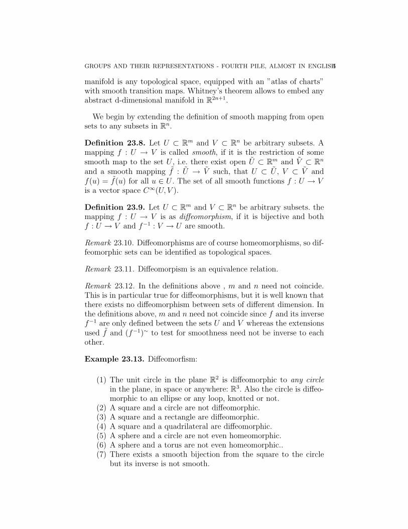
(1) The unit circle in the plane R2 is diffeomorphic to any circlein the plane, in space or anywhere: R3. Also the circle is diffeo-morphic to an ellipse or any loop, knotted or not.

(2) A square and a circle are not diffeomorphic.(3) A square and a rectangle are diffeomorphic.(4) A square and a quadrilateral are diffeomorphic.(5) A sphere and a circle are not even homeomorphic.(6) A sphere and a torus are not even homeomorphic..(7) There exists a smooth bijection from the square to the circle

but its inverse is not smooth.

6 KAREN E. SMITH

Kuva 1: Ympyra and solmu ovat diffeomorfiset

Download ”Differential Topology” by Guillemin and andPollack for free! Download our favourite book at Pdfdataba-se.com. pdfdatabase.com/differential-topology-guillemin-pollack.html. There are other addresses as well. Also solutions to exercisesare available after googleing a bit.

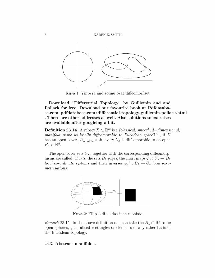
Definition 23.14. A subsetX ⊂ Rm is a (classical, smooth, d−dimensional)manifold, same as locally diffeomorphic to Euclidean spaceRn , if Xhas an open cover {Uλ}λ∈Λ, s.th. every Uλ is diffeomorphic to an openBλ ⊂ Rd.

The open cover sets Uλ , together with the corresponding diffeomorp-hisms are called charts, the sets Bλ pages, the chart maps ϕλ : Uλ → Bλ

local co-ordinate systems and their inverses ϕ−1λ : Bλ → Uλ local para-

metrisations.

!

!

! "

Kuva 2: Ellipsoidi is klassinen monisto

Remark 23.15. In the above definition one can take the Bλ ⊂ Rd to beopen spheres, generalised rectangles or elements of any other basis ofthe Euclidean topology.

23.3. Abstract manifolds.


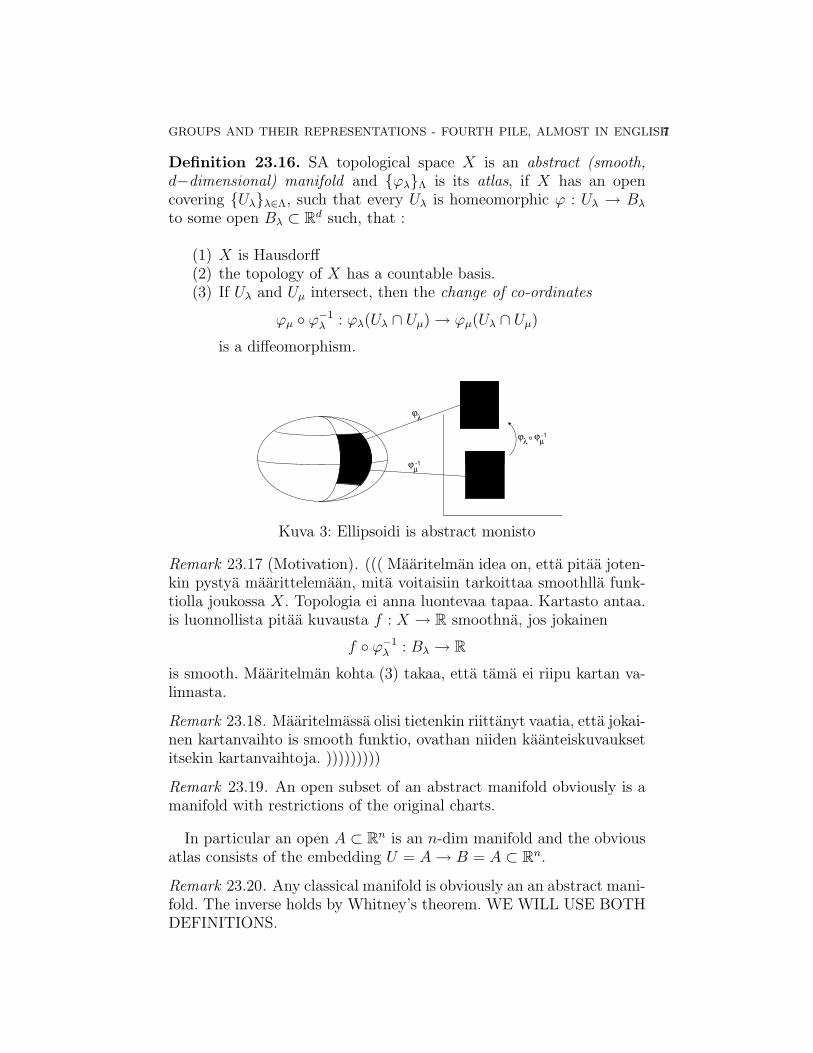
Definition 23.16. SA topological space X is an abstract (smooth,d−dimensional) manifold and {ϕλ}Λ is its atlas, if X has an opencovering {Uλ}λ∈Λ, such that every Uλ is homeomorphic ϕ : Uλ → Bλ

to some open Bλ ⊂ Rd such, that :

(1) X is Hausdorff(2) the topology of X has a countable basis.(3) If Uλ and Uµ intersect, then the change of co-ordinates

ϕµ ◦ ϕ−1λ : ϕλ(Uλ ∩ Uµ)→ ϕµ(Uλ ∩ Uµ)

is a diffeomorphism.

Kuva 3: Ellipsoidi is abstract monisto

Remark 23.17 (Motivation). ((( Maaritelman idea on, etta pitaa joten-kin pystya maarittelemaan, mita voitaisiin tarkoittaa smoothlla funk-tiolla joukossa X. Topologia ei anna luontevaa tapaa. Kartasto antaa.is luonnollista pitaa kuvausta f : X → R smoothna, jos jokainen

f ◦ ϕ−1λ : Bλ → R

is smooth. Maaritelman kohta (3) takaa, etta tama ei riipu kartan va-linnasta.

Remark 23.18. Maaritelmassa olisi tietenkin riittanyt vaatia, etta jokai-nen kartanvaihto is smooth funktio, ovathan niiden kaanteiskuvauksetitsekin kartanvaihtoja. )))))))))

Remark 23.19. An open subset of an abstract manifold obviously is amanifold with restrictions of the original charts.

In particular an open A ⊂ Rn is an n-dim manifold and the obviousatlas consists of the embedding U = A→ B = A ⊂ Rn.

Remark 23.20. Any classical manifold is obviously an an abstract mani-fold. The inverse holds by Whitney’s theorem. WE WILL USE BOTHDEFINITIONS.

8 KAREN E. SMITH

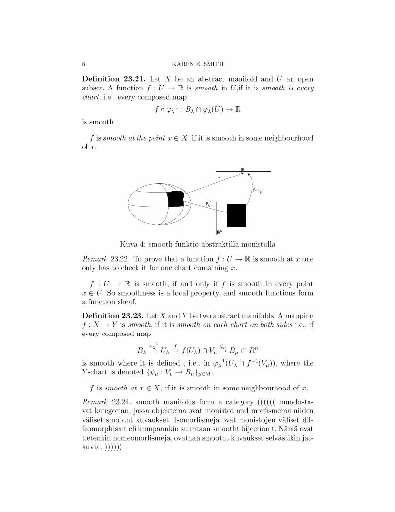
Definition 23.21. Let X be an abstract manifold and U an opensubset. A function f : U → R is smooth in U ,if it is smooth is everychart, i.e.. every composed map

f ◦ ϕ−1λ : Bλ ∩ ϕλ(U)→ R

is smooth.

f is smooth at the point x ∈ X, if it is smooth in some neighbourhoodof x.

Kuva 4: smooth funktio abstraktilla monistolla

Remark 23.22. To prove that a function f : U → R is smooth at x oneonly has to check it for one chart containing x.

f : U → R is smooth, if and only if f is smooth in every pointx ∈ U . So smoothness is a local property, and smooth functions forma function sheaf.

Definition 23.23. Let X and Y be two abstract manifolds. A mappingf : X → Y is smooth, if it is smooth on each chart on both sides i.e.. ifevery composed map

Bλ

ϕ−1λ→ Uλ

f→ f(Uλ) ∩ Vµψµ→ Bµ ⊂ Rn

is smooth where it is defined , i.e.. in ϕ−1λ (Uλ ∩ f−1(Vµ)), where the

Y -chart is denoted {ψµ : Vµ → Bµ}µ∈M .

f is smooth at x ∈ X, if it is smooth in some neighbourhood of x.

Remark 23.24. smooth manifolds form a category (((((( muodosta-vat kategorian, jossa objekteina ovat monistot and morfismeina niidenvaliset smootht kuvaukset. Isomorfismeja ovat monistojen valiset dif-feomorphismt eli kumpaankin suuntaan smootht bijection t. Nama ovattietenkin homeomorfismeja, ovathan smootht kuvaukset selvastikin jat-kuvia. ))))))


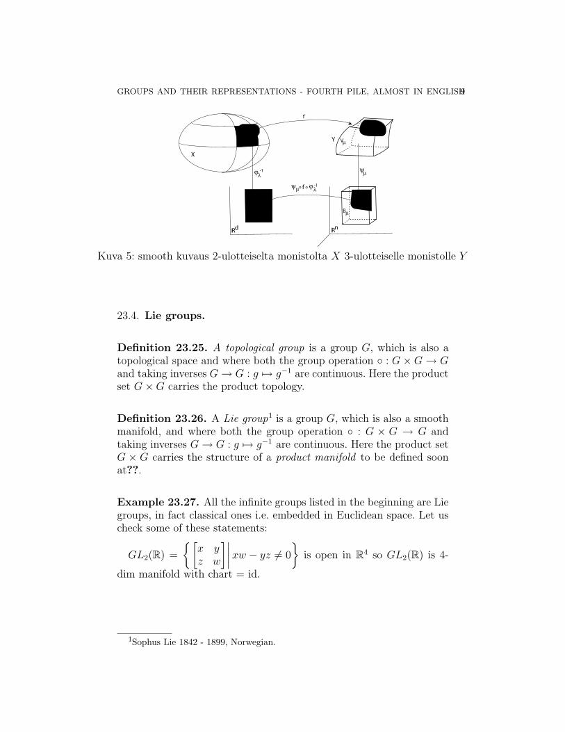
Kuva 5: smooth kuvaus 2-ulotteiselta monistolta X 3-ulotteiselle monistolle Y

23.4. Lie groups.

Definition 23.25. A topological group is a group G, which is also atopological space and where both the group operation ◦ : G×G→ Gand taking inverses G→ G : g 7→ g−1 are continuous. Here the productset G×G carries the product topology.

Definition 23.26. A Lie group1 is a group G, which is also a smoothmanifold, and where both the group operation ◦ : G × G → G andtaking inverses G→ G : g 7→ g−1 are continuous. Here the product setG × G carries the structure of a product manifold to be defined soonat??.

Example 23.27. All the infinite groups listed in the beginning are Liegroups, in fact classical ones i.e. embedded in Euclidean space. Let uscheck some of these statements:

GL2(R) =

{[x yz w

]∣∣∣∣xw − yz 6= 0

}is open in R4 so GL2(R) is 4-

dim manifold with chart = id.

1Sophus Lie 1842 - 1899, Norwegian.

10 KAREN E. SMITH

SL2(R) =

{[x yz w

]∣∣∣∣xw − yz = 1

}is a closed set in Euclidean space

R4. Let us check directly by definition that it is a manifold. Choose:

Ux =

{[x yz w

]∣∣∣∣xw − yz = 1, x 6= 0

}Uy =

{[x yz w

]∣∣∣∣xw − yz = 1, y 6= 0

}Uz =

{[x yz w

]∣∣∣∣xw − yz = 1, z 6= 0

}Uw =

{[x yz w

]∣∣∣∣xw − yz = 1, w 6= 0

}And choose chart maps

ϕx : Ux → Bx = {(x, y, z) ∈ R3∣∣ x 6= 0} :

[x yz w

]7→ (x, y, z),

ϕy : Uy → By = {(x, y, w) ∈ R3∣∣ y 6= 0} :

[x yz w

]7→ (x, y, w),

ϕz : Uz → Bz = {(x, z, w) ∈ R3∣∣ z 6= 0} :

[x yz w

]7→ (x, z, w),

ϕw : Uw → Bw = {(y, z, w) ∈ R3∣∣ w 6= 0} :

[x yz w

]7→ (y, z, w),

such, that the deleted co-ordinate can always be calculated from theothers by xw − yz = 1, which gives local parametrizations:

ϕ−1x : Bx → Ux : (x, y, z) 7→

[x yz yz+1

x

],

ϕ−1y : By → Uy : (x, y, w) 7→

[x y

xw−1y

w

],

ϕ−1z : Bz → Uz : (x, z, w) 7→

[x xw−1

zz w

],

ϕ−1w : Bw → Uw : (y, z, w) 7→

[yz+1w

yz w

].

All these are obviously smooth, so diffeomorfisms. By the classical def.,SL2(R) is a smooth 3-dim manifold.

To learn it, let us calculate the coordinate transition functions also:

Ux ∩ Uy =

{[x yz w

]∣∣∣∣xw − yz = 1, x 6= 0, y 6= 0

}


ϕx(Ux ∩ Uy) = {(x, y, z) ∈ R3∣∣ x 6= 0, y 6= 0} ⊂ Bx

ϕy ◦ ϕ−1x : ϕy(Ux ∩ Uy)

ϕ−1x→ Ux ∩ Uy

ϕy→ ϕy(Ux ∩ Uy) ⊂ By :

(x, y, z) 7→[x yz yz+1

x

]7→ (x, y,

yz + 1

x).

This is a smooth bijection. The other 7 are similar.

In a similar fashion, SL2(C) =

{[x yz w

]∈ C2×2

∣∣∣∣xw − yz = 1

}is a

complex manifold, since rational functions are holomorphic.

The other Lie groups will be considered later or in the exercises.

(Finite sets can be considered 0-dimensional manifolds!)

24. Tangent spaces and tangent mappings

The idea of a tangent space: Let ψ(x) = ψ(x1, . . . , xd) be a point in aclassical manifold M ⊂ Rn. Here ψ : B → X is a local parametrisation.Since a local parametrisation is smooth, it has a derivative at x =(x1, . . . , xd) ∈ B ⊂ Rd. This derivative is a linear mapping L = dxψ :Rd → Rn giving a close approximation to y 7→ ψ(y) in a neighbourhoodof x. So its image set, the ”plane” ψ(x) + L(Rd) is locally a goodapproximation to ψ(B), which is a piece of the manifold M .

Instead of the ”geometrically intuitive” tangent space, we will - fornotational simplicity, consider the subspace parallel to it and call thesubspace L(Rd) the tangent space to M at ψ(x).

24.1. The derivative of a smooth function. The formal defini-tion for a derivative can be found in any textbook.

The derivative is a linear mapping its matrix in any basis, often thestandard basis of Rn, is its Jacobian matrix consisting of its partial(same as directional!) derivatives

dbf (h) = limt→0

f(b+ th)− f(b)

tin the well known way.

12 KAREN E. SMITH

We will occasionally use some of the following terminology. A markedsmooth manifold (M,x0) is smooth manifold, with a distinguished pointx0 ∈M . A morphism of marked manifolds f : (M,x0)→ (N, y0) sameas a smooth mapping between marked manifolds (M,x0) and (N, y0)is a smooth map M → N mapping x0 7→ y0.

The tangent space TxM of a smooth marked manifold (M,x0) willbe defined so that it will have the following properties:

To every morphism of marked manifolds

f : (M,x0)→ (N, y0)

there is a linear mapping

Tx0f : (M,x0)→ (N, y0)

and this correspondence is a functor, i.e.

Tx0(f ◦ g) = Tg(x0)f ◦ Tx0g,

whenever the composed morphism f ◦ g is defined at x0. The tangentmapping same as derivative of f : (M,x) → (N, y) is this linearmapping Tx0f : (M,x0)→ (N, y0). [[[something is still missing: maybewe should say that the tangent mapping is the derivative wheneverthe derivative is already defined. note: this was no definition, just aprologue?]]]]

Definition 24.1. Consider a point x0 = ψ(x) = ψ(x1, . . . , xd), in ad-dimensional manifold M ⊂ Rn where ψ : B → X is local parametri-sation. Since a local parametrisation is smooth, it has a derivative atx = (x1, . . . , xd) ∈ B ⊂ Rd. The tangent space of the manifold M atx0 = ψ(x) is the image space Tx0(M) = dxψ(Rd).

Definition 24.2. . Consider a smooth mapping between marked ma-nifolds: f : (M,x) → (N, y) and a local paramterisations at the mar-ked points ψ : B → U , and assume b 7→ x and ϕ : U ′ → B′, wherey 7→ b′ ∈ B′ and : M ⊂ Rn, B ⊂ Rd, N ⊂ Rn, B′ ⊂ Rd′ .

The tangent mapping same as derivative of the mapping f is thederivative

db(ϕ ◦ f ◦ ψ) : Rd → Rd′ .

Remark 24.3. The definition above is not complete: One has to proveexistence and uniqueness ei independence of the choice of charts. Letus do it. Before doing the general case, let us consider an example:


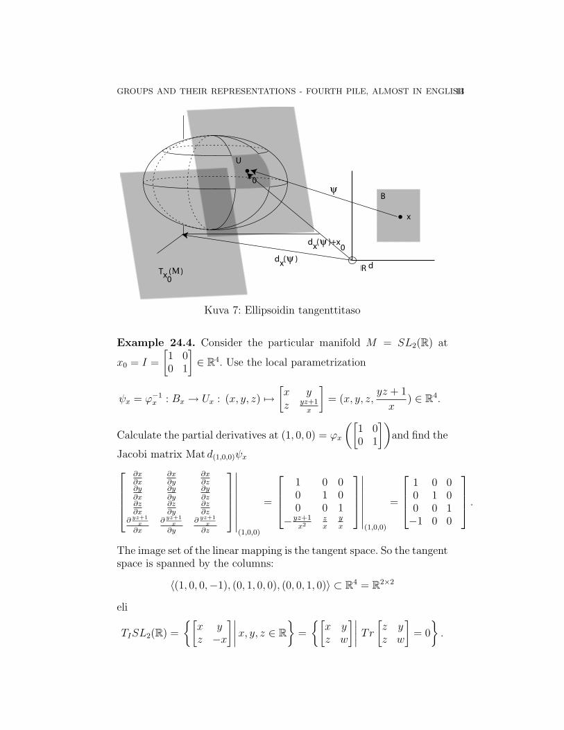
Kuva 7: Ellipsoidin tangenttitaso

Example 24.4. Consider the particular manifold M = SL2(R) at

x0 = I =

[1 00 1

]∈ R4. Use the local parametrization

ψx = ϕ−1x : Bx → Ux : (x, y, z) 7→

[x yz yz+1

x

]= (x, y, z,

yz + 1

x) ∈ R4.

Calculate the partial derivatives at (1, 0, 0) = ϕx

([1 00 1

])and find the

Jacobi matrix Mat d(1,0,0)ψx∂x∂x

∂x∂y

∂x∂z

∂y∂x

∂y∂y

∂y∂z

∂z∂x

∂z∂y

∂z∂z

∂ yz+1x

∂x

∂ yz+1x

∂y

∂ yz+1x

∂z

∣∣∣∣∣∣∣∣∣(1,0,0)

=

1 0 00 1 00 0 1

−yz+1x2

zx

yx

∣∣∣∣∣∣∣∣(1,0,0)

=

1 0 00 1 00 0 1−1 0 0

.The image set of the linear mapping is the tangent space. So the tangentspace is spanned by the columns:

〈(1, 0, 0,−1), (0, 1, 0, 0), (0, 0, 1, 0)〉 ⊂ R4 = R2×2

eli

TISL2(R) =

{[x yz −x

]∣∣∣∣x, y, z ∈ R}

=

{[x yz w

]∣∣∣∣ Tr [z yz w

]= 0

}.

14 KAREN E. SMITH

Similarly ⊂ R4, for instance by the parametrization

ψw = ϕ−1w : Bw → Uw : (y, z, w) 7→

[yz+1w

yz w

]one finds at (y, z, w) = (0, 0, 1) derivative

zw

yw−1+w

w2

1 0 00 1 00 0 1

∣∣∣∣∣∣∣∣(0,0,1)

=

0 0 −11 0 00 1 00 0 1

,from where one finds the tangent space to be

TISL2(R) =

{[−w yz w

]∣∣∣∣ y, z, w ∈ R}

=

{[x yz w

]∣∣∣∣ Tr [z yz w

]= 0

},

which is the same set that was found by the first parametrization. .

In fact it is intuitively clear why both parametrizations should givethe same tangent space. The charts ϕi and their inverses, the localprametrizations ϕ−1

i = ψi form a commutative diagram

R3 ⊃ Bx ⊃ ϕx(Ux ∩ Uw)ψx−→ Ux ∩ Uw

η = ϕw ◦ ψx ↓ · ↓ IR3 ⊃ Bw ⊃ ϕw(Ux ∩ Uw)

ψw−→ Ux ∩ Uw

The chart transition map η = ϕw◦ψx is diffeomorphism, and η(1, 0, 0) =

ϕw

([1 00 1

])= (0, 0, 1). The maps in the diagram are smooth. By

taking derivatives we get the diagram

R3d(1,0,0)ψx−→ R4

d(1,0,0)η = d(1,0,0)(ϕw ◦ ψx) ↓ · ↓ identical mapping

R3d(0,0,1)ψw−→ R4

Here one observes immediately d(0,0,1)ψw(R3) ⊂ d(1,0,0)ψx(R3). ”=”follows from symmetry or from the fact that the transition map η is adiffeomorphism, so its derivative is bijective.

Theorem 24.5. The tangent space of a manifold at a given point doesnot depend on the choice of local coordinatization.


Todistus. Given above!!! �

Remark 24.6. Remember, a Lie group is a group and a manifold, wherethe mappings G × G → G : (x, y) 7→ xy and x 7→ x−1 are smooth.Here the product set carries both the product group structure andthe product manifold structure, the latter having products and productmappings of the original charts as charts.

Definition 24.7. A Lie group map also called a homomorpism (ofLie groups) is a smooth group homomorphism, similarly a Lie groupisomorphism is a smooth isomorphism between Lie groups and whoseinverse is also smooth.

Remark 24.8. Compositions of Lie group maps are Lie group maps, soLie groups form a category.

Example 24.9. (1) G = (R,+) is Lie group, since R × R → R :(x, y) 7→ x+ y and R→ R : x 7→ −x are smooth.

(2) The rotation group / circle S1 is a Lie group, when it is identifiedwith the circle as a manifold:

{(x, y) ∈ R2∣∣ x2 + y2 = 1} = {(cos 2πα, sin 2πα)

∣∣ α ∈ R},

which leads to identifying its group multiplication with

(cos 2πα, sin 2πα) ◦ (cos 2πβ, sin 2πβ) = (cos 2π(α + β), sin 2π(α + β))

and choosing for local parametrizations at (cos 2πα, sin 2πα) the smoothmappings

ψ :]α− ε, α + ε[→ S1

θ 7→ (cos 2πθ, sin 2πθ).

Check smoothness of group operations in S1:

]α− ε, α + ε[×]β − ε, β + ε[ψ×ψ′−→ S1 × S1 ◦→ S1 ϕ−→]α + β − 2ε, α + β + 2ε[

(θ, θ′)ψ×ψ′7→ ((cos 2πθ, sin 2πθ), (cos 2πθ′, sin 2πθ′))

◦7→◦7→ (cos 2π(θ + θ′), sin 2π(θ + θ′))

ϕ7→ θ + θ′.

Remark 24.10. Notice: Above we also got an example of group map:

ι : (R,+)→ S1 : θ 7→ (cos 2πθ, sin 2πθ)

is clearly a group homomorphism and we just proved it to be smoothalso. It is not injective, hence no isomorphism.

16 KAREN E. SMITH

Example 24.11. More Lie group maps:

(1) Since SO(n) ⊂ SL(n) ⊂ GL(n), and all have usual matrix mul-tiplication as the group operation and all carry the classical manifoldstructure inherited from R2n, so the inclusion mappings SO(n)→ SL(nand SL(n)→ GL(n) are Lie group maps.

(2) The circle group S1 consists of rotations of the plane, also in thefollowing sense:

S1 → SOR(2) : (cos 2πθ, sin 2πθ) 7→[cos 2πθ − sin 2πθsin 2πθ cos 2πθ

]is a Lie group isomorphism. Here the matrix group is a classical mani-fold in R4.

Also the group U(1) = {z ∈ C∣∣ |z| = 1} ⊂ C with complex number

multiplication and the manifold structure coming from the identifica-tion C = R2 is isomorphic to S1. Details left as exercise.

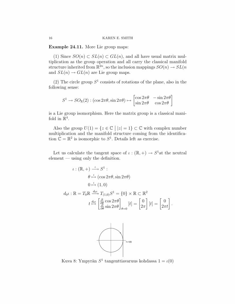
Let us calculate the tangent space of ι : (R,+) → S1at the neutralelement — using only the definition.

ι : (R,+)ι−→ S1 :

θι7→ (cos 2πθ, sin 2πθ)

0ι7→ (1, 0)

d0ι : R = T0Rd0ι−→ T(1,0)S

1 = {0} × R ⊂ R2

td0ι7→[∂∂θ

cos 2πθ∂∂θ

sin 2πθ

]θ=0

[t] =

[0

2π

][t] =

[0

2πt

].

Kuva 8: Ympyran S1 tangenttiavaruus kohdassa 1 = ι(0)


25. Representations of Lie groups

Remark 25.1. In the following ”vector spaces” will be finite dimensio-nal, real — unless otherwise stated..

Definition 25.2. A representation of a Lie group G is a representationof the group G in a vector space V ( a group homomorphism G →GL(V )) , also a smooth mapping. Ie A Lie group representation is thesame thing as a lie group mapping ρ : G→ GL(V ).

Example 25.3. (1) If course , the Lie groups which already by de-finition consist of linear mappings together with composition (matrixmultiplication), like GL(n), O(n), SL(n) etc. have a tautological repre-sentation, which is just the identical mapping of the group.

(2) The group of invertible numbers (R∗, ·) has many representations,already in dimension 2 i.e.. in R2:

(1) multiplication by the number itself: λ 7→[λ 00 λ

]∈ GL(2)

(2) multiplication by the square of number itself:: λ 7→[λ2 00 λ2

]∈

GL(2)

(3) Generalisations of the above: λ 7→[λm 00 λn

]∈ GL(2); (m,n ∈

Z)

(4) Action of λ ∈ R∗ as by multiplication with ‖λ‖. : λ 7→[|λ|α 0

0 |λ|β]

All these are reducible, in fact already ”reduced”. The group is abe-lian. The irreducible representations of the abelian group mentionedabove are one dimensional. Exercise: are there any higher dimensionalirreducible representations?

26. Linear and multilinear algebra

26.1. Bilinear mappings.

Definition 26.1. Let V, W and U be vector spaces and Ftheir coef-ficient field. A mapping B : V × W → U is called bilinear, if bothpartial mappings

B(v, ·) : W → U : w 7→ B(v, w)

18 KAREN E. SMITH

and

B(·, w) : V → U : v 7→ B(v, w)

are linear. Examples:

Example 26.2. Almost all mappings called ”products” in linear al-gebra are in fact bilinear:

(1) multiplication in R xy(2) multiplication in C zz′

(3) multiplication of vectors by numbers λv(4) inner product of vectors (v|w)(5) matrix multiplication AB,(6) in particular multiplication of vectors by matrices Ax(7) evaluation of linear mappings at points Tv,(8) in particular evaluation of linear forms < v|u′〉(9) point-wise product of functions fg

(10) tensor product of vectors x⊗ y(11) tensor product of linear mappings T ⊗ S

26.2. Tensor product of 2 vector spaces.

Definition 26.3. A subset of a vector space K ⊂ V is free (sameas its elements are linearly independent, if the only way to express 0as a linear combination of the vectors is the trivial combination 0 =∑n

j=1 0vj, vj ∈ K, n ∈ N.

A subset of a vector space K ⊂ V spans the space V , if every vectorv ∈ V is the linear combination v =

∑nj=1 λjvj; vj ∈ K, n ∈ N of some

vectors in K.

A (Hamel) basis of a vector space V is a free set K ⊂ V ,spanningV .

Remark 26.4. A set K ⊂ V is a basis of V if and only if every vectorv ∈ V can be expressed as a linear combination v =

∑nj=1 λjvj, where

λj ∈ F, vj ∈ K, n ∈ N, in exactly one way.

Liner combinations v =∑n

j=1 λjvj, where λj ∈ F, vj ∈ K, n ∈ N,are often denoted in short hand: v =

∑K λkk, where — of course —

only finite many λk are distinct of 0.

All bases of the same vector space have the same cardinality. A vectorspace is d-dimensional when it has a basis with d elements. The axiom of


choice implies that every vector space has a basis — generally infinite,of course.

A linear mapping is uniquely defined by the images of the basis ele-ments, and the se images can be any vectors. In particular, in the finitedimensional case, representing linear mappings by matrices is based onthis fact. Similarly, a bilinear mapping B : V ×W → U is complete-ly determined by the values B(k, l), where k goes through a basis ofK of V and a basis L of W . This is so, since B (

∑K λkk,

∑L µll) =∑

K×L λkµlkl.

Definition 26.5. The The free vector space spanned by set K is avector space F(K) whose basis is K.

Remark 26.6. The free vector space spanned by K is unique up toisomorphism. Also, it exists: Every set K spans some vector space,since a vector space with basis K can be constructed as follows: FK ={f∣∣ f is a function K → F}. Obviously FK is a vector space. Define

F(K) = F(K) = {f ∈ FK∣∣ f(k) 6= 0 for only finitely many k ∈ K}.

Finally, identify K with the subset K ⊂ F(K) by identifying the elementl ∈ K with the mapping k 7→ δlk, where δkl=1, if k = l and 0 else. Inthis notation, every f ∈ V is a finite sum2 f =

∑k∈K λkk, where

λk = f(k).

All in all every vector space is a free vector space and every set isthe basis of some vector space.3

Remark 26.7. Next we define the tensor product of two vector spacesV and W as consisting of a space V ⊗ W and a bilinear mapping

V ×W ⊗→ V ⊗W . There exist several commonly used definitions for thetensor product, preferences depending on intended use. The followingwill be either included in the definition or proven as theorems:

(1) The tensor product of two vector spaces V and W is the mostgeneral i.e. universal bilinear mapping in V ×V in the following sense:Each bilinear B : V ×W → U can be factored as B = L ◦ ⊗, where

2only finitely many terms 6= 0!3If the coefficient field of the vector space is replaced by just a ring(!), we arrive

at the concept of a module. A free module is defined much like a free vector space.It turns out that not every module is free.

20 KAREN E. SMITH

L : V ⊗W → U is a bilinear mapping depending uniquely (!) on B.

V ×W ⊗−→ V ⊗WB

↘ ↓ LU

We will have to prove to existence and uniqueness of such a bilinearmapping ⊗.

(2) The tensor product of two vector spaces V = F(K) and W = F(L)

is the free vector space V ⊗W = F(K) ⊗ F(L) = F(K×L) equipped withthe bilinear mapping

V ×W ⊗→ V ⊗W,mapping the pair of basis vectors (k, l) is mapped to the basis vector(k, l) ∈ V ⊗W = F(K×L). In particular dim(V ⊗W ) = dimV · dimW .The basis vectors in the tensor product are usually denoted by⊗(k, l) =k ⊗ l . Therefore, the elements of the tensor product V ⊗W generallyare finite sums of the form ∑

(k,l)∈K×L

λk,l k ⊗ l

and the bilinear mapping ⊗ : V ×W → V ⊗W is

(∑k∈K

λk k)⊗ (∑l∈L

µl l) =∑

(k,l)∈K×L

λkµl k ⊗ l.

Bilinearity is expressed by:

(v + v′)⊗ w = v ⊗ w + v′ ⊗ wλ · (v ⊗ w) = (λ · v)⊗ w

v ⊗ (w + w′) = v ⊗ w + v ⊗ w′

λ · (v ⊗ w) = v ⊗ (λ · w)

for all v, v′, ∈ V, w,w′ ∈ W, λ ∈ F.

These properties might not make it evident that the tensor product⊗ : V × W → V ⊗ W is unique up to isomorphism, in particularindependent of the choice of a basis. 4

The following definition of tensor product includes an explicit con-struction without referring to any basis. This definition also generalisesto outer and symmetric products of spaces

4Also, definitions should generally be ” coordinate free” to avoid such questionsas well as the questions of existence of basis, which was solved above.


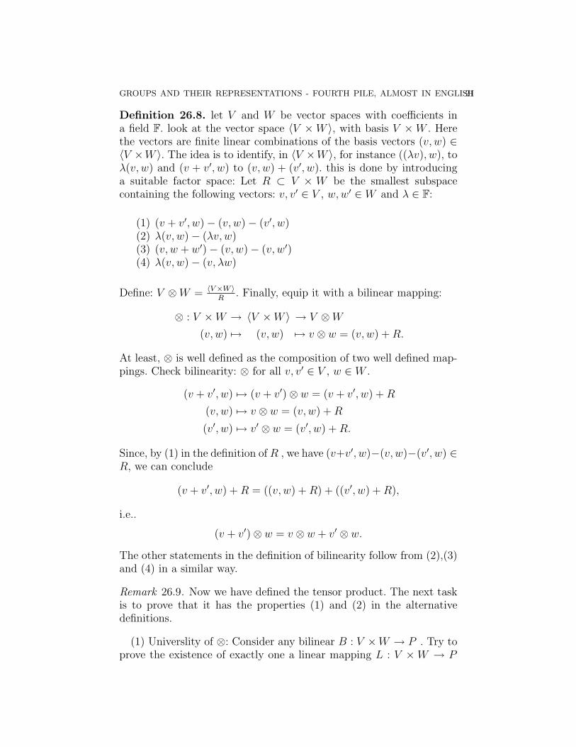
Definition 26.8. let V and W be vector spaces with coefficients ina field F. look at the vector space 〈V ×W 〉, with basis V ×W . Herethe vectors are finite linear combinations of the basis vectors (v, w) ∈〈V ×W 〉. The idea is to identify, in 〈V ×W 〉, for instance ((λv), w), toλ(v, w) and (v + v′, w) to (v, w) + (v′, w). this is done by introducinga suitable factor space: Let R ⊂ V × W be the smallest subspacecontaining the following vectors: v, v′ ∈ V , w,w′ ∈ W and λ ∈ F:

(1) (v + v′, w)− (v, w)− (v′, w)(2) λ(v, w)− (λv, w)(3) (v, w + w′)− (v, w)− (v, w′)(4) λ(v, w)− (v, λw)

Define: V ⊗W = 〈V×W 〉R

. Finally, equip it with a bilinear mapping:

⊗ : V ×W → 〈V ×W 〉 → V ⊗W(v, w) 7→ (v, w) 7→ v ⊗ w = (v, w) +R.

At least, ⊗ is well defined as the composition of two well defined map-pings. Check bilinearity: ⊗ for all v, v′ ∈ V , w ∈ W .

(v + v′, w) 7→ (v + v′)⊗ w = (v + v′, w) +R

(v, w) 7→ v ⊗ w = (v, w) +R

(v′, w) 7→ v′ ⊗ w = (v′, w) +R.

Since, by (1) in the definition of R , we have (v+v′, w)−(v, w)−(v′, w) ∈R, we can conclude

(v + v′, w) +R = ((v, w) +R) + ((v′, w) +R),

i.e..

(v + v′)⊗ w = v ⊗ w + v′ ⊗ w.

The other statements in the definition of bilinearity follow from (2),(3)and (4) in a similar way.

Remark 26.9. Now we have defined the tensor product. The next taskis to prove that it has the properties (1) and (2) in the alternativedefinitions.

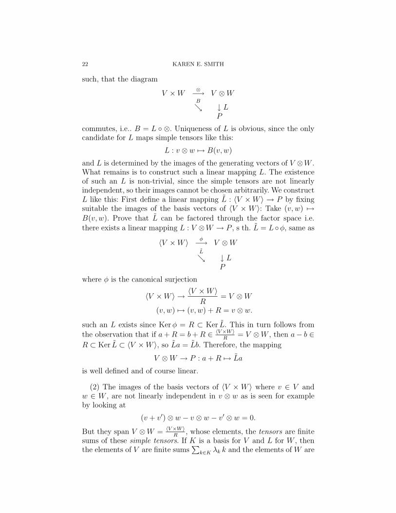
(1) Universlity of ⊗: Consider any bilinear B : V ×W → P . Try toprove the existence of exactly one a linear mapping L : V ×W → P

22 KAREN E. SMITH

such, that the diagram

V ×W ⊗−→ V ⊗WB

↘ ↓ LP

commutes, i.e.. B = L ◦ ⊗. Uniqueness of L is obvious, since the onlycandidate for L maps simple tensors like this:

L : v ⊗ w 7→ B(v, w)

and L is determined by the images of the generating vectors of V ⊗W .What remains is to construct such a linear mapping L. The existenceof such an L is non-trivial, since the simple tensors are not linearlyindependent, so their images cannot be chosen arbitrarily. We constructL like this: First define a linear mapping L : 〈V ×W 〉 → P by fixingsuitable the images of the basis vectors of 〈V × W 〉: Take (v, w) 7→B(v, w). Prove that L can be factored through the factor space i.e.there exists a linear mapping L : V ⊗W → P , s th. L = L ◦φ, same as

〈V ×W 〉 φ−→ V ⊗WL

↘ ↓ LP

where φ is the canonical surjection

〈V ×W 〉 → 〈V ×W 〉R

= V ⊗W

(v, w) 7→ (v, w) +R = v ⊗ w.

such an L exists since Kerφ = R ⊂ Ker L. This in turn follows from

the observation that if a+R = b+R ∈ 〈V×W 〉R

= V ⊗W , then a− b ∈R ⊂ Ker L ⊂ 〈V ×W 〉, so La = Lb. Therefore, the mapping

V ⊗W → P : a+R 7→ La

is well defined and of course linear.

(2) The images of the basis vectors of 〈V ×W 〉 where v ∈ V andw ∈ W , are not linearly independent in v ⊗ w as is seen for exampleby looking at

(v + v′)⊗ w − v ⊗ w − v′ ⊗ w = 0.

But they span V ⊗W = 〈V×W 〉R

, whose elements, the tensors are finitesums of these simple tensors. If K is a basis for V and L for W , thenthe elements of V are finite sums

∑k∈K λk k and the elements of W are


sums∑

l∈L µl l so the elements of the tensor product space are finitesums

(∑k∈K

λk k)⊗ (∑l∈L

µl l) =∑

(k,l)∈K×L

λkµl k ⊗ l =∑

(k,l)∈K×L

ρk,l k ⊗ l.

We have just proved that the tensor products of the original basisvectors span the tensor product space. V ⊗ W . Now we prove theirlinear independence. Let∑

(k,l)∈K×L

λk,l k ⊗ l = 0 ∈ V ⊗W.

By universality of the bilinear mapping ⊗ every bilinear mapping B :V ×W → F corresponds to a unique linear mapping L : V ×W → Pmaking the diagram

V ×W ⊗−→ V ⊗WB

↘ ↓ LF

commutative, i.e.. such that B = L◦⊗. In particular, for every bilinearmapping B : V ×W → F we have

∑(k,l)∈K×L λk,l B(k, l) = 0. But the

images of the pairs of basis vectors cab e chosen freely when setting upa bilinear mapping. Therefore

∑(k,l)∈K×L λk,l Bk,l = 0 for all choices

Bk,l ∈ F, so every λk,l is 0. �

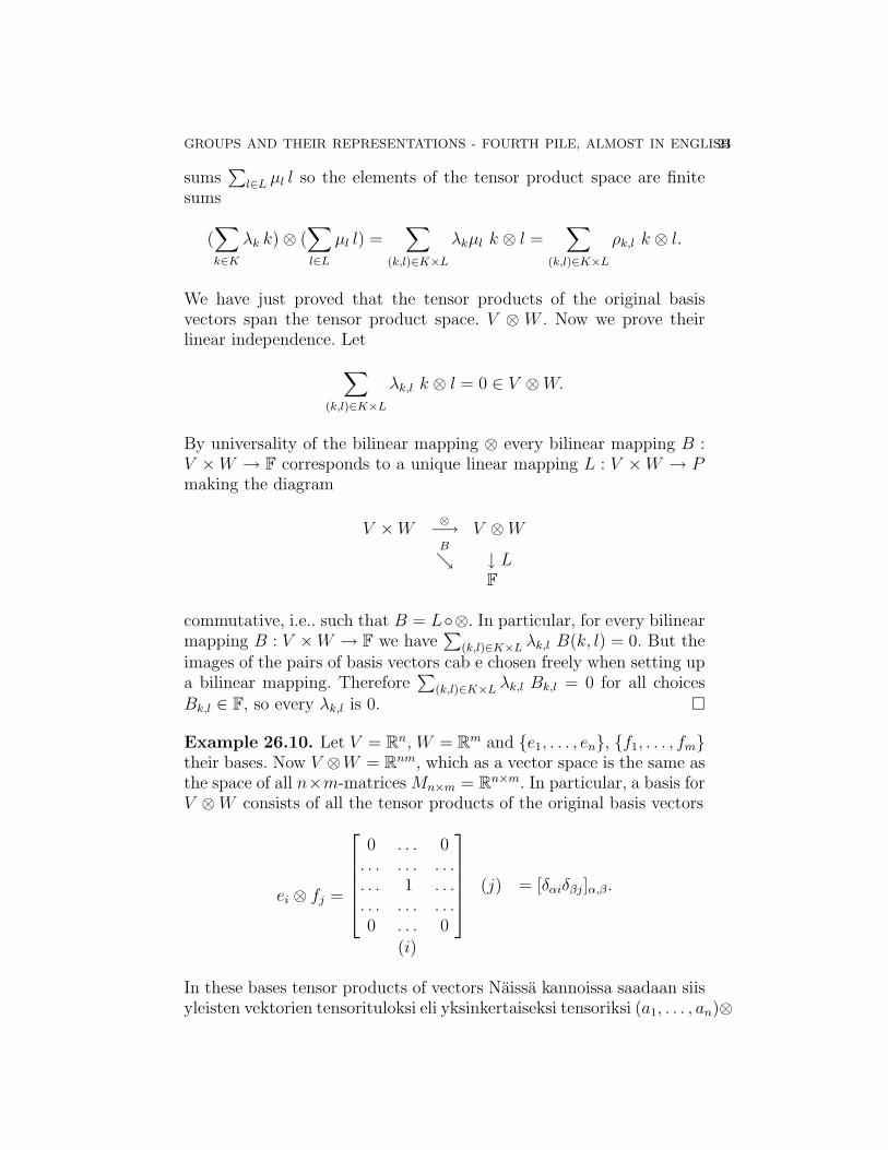
Example 26.10. Let V = Rn, W = Rm and {e1, . . . , en}, {f1, . . . , fm}their bases. Now V ⊗W = Rnm, which as a vector space is the same asthe space of all n×m-matrices Mn×m = Rn×m. In particular, a basis forV ⊗W consists of all the tensor products of the original basis vectors

ei ⊗ fj =

0 . . . 0. . . . . . . . .. . . 1 . . .. . . . . . . . .0 . . . 0

(j)

(i)

= [δαiδβj]α,β.

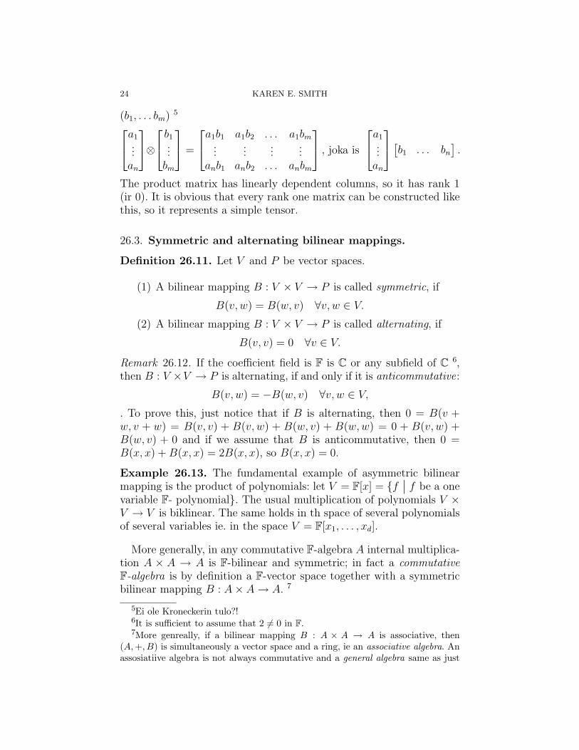
In these bases tensor products of vectors Naissa kannoissa saadaan siisyleisten vektorien tensorituloksi eli yksinkertaiseksi tensoriksi (a1, . . . , an)⊗

24 KAREN E. SMITH

(b1, . . . bm) 5a1...an

⊗ b1

...bm

=

a1b1 a1b2 . . . a1bm...

......

...anb1 anb2 . . . anbm

, joka is

a1...an

[b1 . . . bn].

The product matrix has linearly dependent columns, so it has rank 1(ir 0). It is obvious that every rank one matrix can be constructed likethis, so it represents a simple tensor.

26.3. Symmetric and alternating bilinear mappings.

Definition 26.11. Let V and P be vector spaces.

(1) A bilinear mapping B : V × V → P is called symmetric, if

B(v, w) = B(w, v) ∀v, w ∈ V.(2) A bilinear mapping B : V × V → P is called alternating, if

B(v, v) = 0 ∀v ∈ V.

Remark 26.12. If the coefficient field is F is C or any subfield of C 6,then B : V ×V → P is alternating, if and only if it is anticommutative:

B(v, w) = −B(w, v) ∀v, w ∈ V,. To prove this, just notice that if B is alternating, then 0 = B(v +w, v + w) = B(v, v) + B(v, w) + B(w, v) + B(w,w) = 0 + B(v, w) +B(w, v) + 0 and if we assume that B is anticommutative, then 0 =B(x, x) +B(x, x) = 2B(x, x), so B(x, x) = 0.

Example 26.13. The fundamental example of asymmetric bilinearmapping is the product of polynomials: let V = F[x] = {f

∣∣ f be a onevariable F- polynomial}. The usual multiplication of polynomials V ×V → V is biklinear. The same holds in th space of several polynomialsof several variables ie. in the space V = F[x1, . . . , xd].

More generally, in any commutative F-algebra A internal multiplica-tion A × A → A is F-bilinear and symmetric; in fact a commutativeF-algebra is by definition a F-vector space together with a symmetricbilinear mapping B : A× A→ A. 7

5Ei ole Kroneckerin tulo?!6It is sufficient to assume that 2 6= 0 in F.7More genreally, if a bilinear mapping B : A × A → A is associative, then

(A, +, B) is simultaneously a vector space and a ring, ie an associative algebra. Anassosiatiive algebra is not always commutative and a general algebra same as just


Example 26.14. In R3 the ”cross product” of two vectors is an exampleof an alternating bilinear mapping. A more fundamental example is gi-ven by the determinant of a 2× 2-matrix:

Let V = R2. The mapping associating to a pair of vectors v =

[a11

a21

]and w =

[a12

a22

]the determinant B(v, w) =

∣∣∣∣a11 a12

a21 a22

∣∣∣∣ is an alternating

bilinear mapping V × V → R.

26.4. Multilinear mappings. It is natural to generalise the determi-nant example to Rd. The determinant is linear in the column vectorsand has the value 0, whenever two columns coincide. This gives themotivation to consider alternating multilinear mappings of more than2 variables.

Definition 26.15. Let V1, . . . , Vn and P be vector spaces and F theircommon coefficient field.

(1) The mapping M : V1× · · · × Vn → P is multilinear, in this casen−linear, if its all partial mappings

V1 → P : v1 7→M(v1, . . . , vn),

V2 → P : v2 7→M(v1, . . . , vn),

. . .

Vn → P : vn 7→M(v1, . . . , vn),

are linear.(2) An n-linear mappingM : V n → P is symmetric, ifM(v1, . . . , vn)

does not depend on the order of the variables v1, . . . , vn. Thismeans that for all permutations σ ∈ Sn we have

M(vσ(1), . . . , vσ(n)) = M(v1, . . . , vn)

(3) An n-linear mapping M : V n → P is alternating, if

M(v1, . . . , vn) = 0 whenever vi = vj for some i 6= j.

Remark 26.16. When F is a subfield of C, then a multilinear mappingis alternating if and only if M(v1, . . . , vn) = 0 whenever v1, . . . , vn arelinearly dependent. This is equivalent to saying that the mapping chan-ges sign whenever two variables are interchanged. The classical example

a bilinear mapping, is not always associative. In particular, lien algebras will notbe associative, nor commutative.

26 KAREN E. SMITH

of an alternating multilinear mapping is — as was already mentioned–the determinant considered as a function of its column (or rows)

26.5. Symmetric and outer powers.

Definition 26.17. Let V1×· · ·×Vn be (F-) vector spaces. An n-linearmap ⊗ : V1 × · · · × Vn → W is called the tensor product of the spacesV1, . . . , Vn and denoted W = V1 ⊗ · · · ⊗ Vn, if ⊗ is a universal n-linearmapping in the following sense:

Every n−linear mappings M : V1 ⊗ · · · ⊗ Vn → U can be factoredinto B = L ◦ ⊗, where L : V1 ⊗ · · · ⊗ Vn → U is a linear mappinguniquely determined by the n−linear mapping M .

V1 × · · · × Vn⊗−→ V1 ⊗ · · · ⊗ VnM

↘ ↓ LU

The construction of the tensor product of two spaces can readily begeneralised to the case of several spaces and proves its existence anduniqueness. The same result can be obtained by paying attention tothat V1 ⊗ · · · ⊗ Vn can be defined as (. . . (V1 ⊗ V2) ⊗ · · · ⊗ Vn). Abasis for the tensor product is given by K1 × · · · × Kn, where Kj isa basis of the original space Vj. In particular, the d:th tensor powerRn ⊗ · · · ⊗ Rn = (Rn)⊗d has a basis consisting of all ei1 ⊗ · · · ⊗ eid ,where {e1, . . . , en} is a basis of the original space Rn.

By the same principle that we used the concept of bilinear mappingsfor constructing the tensor product, we can define and construct thesymmetric and alternating (same as outer) powers of a vector spaceusing symmetric and alternating multilinear mappings:

Definition 26.18. Let V be a (F-) vector space A symmetric n-linearmapping · : V × · · · × V = V n → W is the n:th symmetric powerW = SnV , if it is the universal symmetric n-linear mapping in thefollowing sense:

Every symmetric n−linear mapping M : V n → U is of the formM = L◦·, where L : SnV → U is a linear mapping depending uniquelyon the symmetric n−linear mapping M .

V n ·−→ SnVM

↘ ↓ LU


The existence of a symmetric power is proved by construction. Thiscan be done using bases and/or factor spaces. We skip the constructionsince the following construction of the outer power is almost identical.We just remark that a basis for the symmetric power is given by allproducts of the original basis vectors ei1 · · · · · eid , where i1 ≤ · · · ≤ in,and the original index set I is ordered.

Example 26.19. Let V={degree 1 homogenous polynomials of n variables} =〈x1, . . . , xn〉. In this case SdV = { degree d homogeneous polynomialsof n variables}, for example

S2V = 〈x21, x1x2, x1x2, . . . x1xn, x

22, x2x3, . . . , . . . x

2n〉.

In this example the symmetric product is the same thing as the ”formalproduct” of polynomials.

Definition 26.20. Let V be a (F-) vector space. An alternating n-linear mapping ∧ : V × · · · × V = V n → W is called the n:th outerpower of the space V and denoted W = ΛnV , if it is the universalalternating n-linear mapping :

Each alternating n−linear mapping M : V n → U is of the formM = L ◦ ∧, where L : ΛnV → U is a linear mapping depending onlyon the alternating n−linear mapping M .

V n ∧−→ ΛnVM

↘ ↓ LU

The existence of an outer power is proved by constructing it. Forsimplicity, we do it for n = 2 only. Like above in the construction ofthe tensor product, we begin by considering the free vector space 〈V 2〉,which has all of V 2 as basis. Next define the subspace R, spanned bythe ”relations” mentioned above in the tensor product construction,and one new. This means: R ⊂ V 2 is the smallest vector subspacecontaining the following vectors: for all v, v′w,w′ ∈ V and λ ∈ F:

(1) (v + v′, w)− (v, w)− (v′, w)(2) λ(v, w)− (λv, w)(3) (v, w + w′)− (v, w)− (v, w′)(4) λ(v, w)− (v, λw)(5) (v, w) + (v, w)

28 KAREN E. SMITH

Now the factor space Λ2V = 〈V 2〉R

has the universal property definingthe outer power, when equipped with the bilinear mapping

∧ : V × V → 〈V 2〉 → Λ2V

(v, w) 7→ (v, w) 7→ v ∧ w = (v, w) +R.

follows from condition (5)). We sum up the properties of ∧: bilinearity

λ · (x ∧ y) = (λ · x) ∧ y = x ∧ (λ · y)

(x+ y) ∧ z = x ∧ z + y ∧ zx ∧ (z + w) = x ∧ z + x ∧ w

and alternation:v ∧ w = −w ∧ v.

An outer power satisfying the universal property does exist.

The images of the pairs ei ∧ ej of original basis vectors of V have

images ei∧ej spanning all of Λ2V = 〈V×W 〉R

, so the elements of this spaceare the finite sums of these generators. If the basis K of V is an ordered,then already the products , ek∧el with k < l, span Λ2V , since ek∧el = 0,for k = l and ek ∧ el = −el ∧ ek, where k > l. Linear independence ofthe remaining basis vector candidates is proven essentially in the sameway as we did for the basis of the tensor product.

the basis becomes {ek ∧ el∣∣ k < l} = {e1 ∧ e2, e1 ∧ e3, e1 ∧ e4, . . . e1 ∧

ed, e2 ∧ e3, e2 ∧ e4, . . . e2 ∧ ed, e3 ∧ e4, . . . , . . . ed−1 ∧ ed, }, so dim(Λ2V ) =12n(n− 1).

Example 26.21. Take V = Rn with basis {e1, . . . , en}. NowΛ2V canbe identifies a as a vector space with the space of all anti-symmetricn× n-matrices.

Remark 26.22. Similar considerations can be carried through for higherpowers ΛnV . In particular, if V has its basis K ordered, then the basisvectors for ΛnV can be taken to be the outer products of the originalbasis vectors, ek1 ∧ ek2 ∧ · · · ∧ ekd , withk1 < k2 < · · · < kd.

Example 26.23. By what was just proved, ΛdRd is one dimensionalwith one basis vector being for instance e1 ∧ e2 ∧ · · · ∧ ed. Rememberthat the determinant of a n × n-matrix is an alternating multilinearmapping from the column vectors to the ground field R.

(Rn)n∧−→ ΛnRn ∼ R

det

↘ ↓ L = λ·R


We notice that the determinant is, up to a multiplicative constant,the only alternating n-linear mapping from n-dimensional space to thenumbers. The same holds for any ground field F.

27. Tensor products of representations

Example 27.1. In example ?? we mentioned the space SdV of homo-geneous polynomials of degree d and n variables. A special case is

S2V = 〈x21, x1x2, x1x2, . . . x1xn, x

22, x2x3, . . . , . . . x

2n〉.

A linear change of co-ordinates is a linear mapping

SdV → SdV : P 7→ P ◦ L,

where L : Rn → Rn is linear.8 If ρ : G → GLn(R) is a representation,then also g 7→ (P 7→ P ◦ρ(g)) is a representation of G. This is a specialcase of the following general construction.

27.1. Induced representations. 9 By definition, a representation ofa Lie group G in a vector space V is a smooth group homomorphismG→ GL(V ).

Definition 27.2. Let ρ and ρ′ : G → GL(V ) be representations of agroup G in finite dimensional spaces V and W . Then the following arerepresentations

(1) ρ⊗ ρ′ : g 7→ (ρ⊗ ρ′)g : V ⊗W → V ⊗W : u⊗ w 7→ ρgu⊗ ρgv.(2) ρ · ρ′ : g 7→ (ρ · ρ′)g : S2V → S2V : u · w 7→ ρgu · ρ′gv.

(3) ρ ∧ ρ′ : g 7→ (ρ ∧ ρ′)g : S2V → S2V : u ∧ w 7→ ρgu ∧ ρ′gv.

Here linear mappings are determined by giving the images of thebasis vectors.

Example 27.3. The tautological representation of the group G =GL2(R) acts in R2. It induces a representation in the outer productλ2(R2). The induced representation is one dimensional with basis vectore1∧e2. Let us find an explicit expression for it: An element of the group

8Strictly speaking, polynomials are not functions but can often be interpreted assuch.

9Seems, in Serre’s book, induced representations are something different.

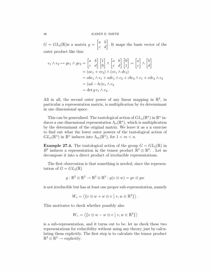
30 KAREN E. SMITH

G = GL2(R)is a matrix g =

[a bc d

]. It maps the basis vector of the

outer product like this:

e1 ∧ e2 7→ ge1 ∧ ge2 =

[a bc d

] [10

]∧[a bc d

] [01

]=

[ac

]∧[bd

]= (ae1 + ce2) ∧ (ce1 ∧ de2)

= abe1 ∧ e1 + ade1 ∧ e2 + cbe2 ∧ e1 + cde2 ∧ e2

= (ad− bc)e1 ∧ e2

= det g e1 ∧ e2.

All in all, the second outer power of any linear mapping in R2, inparticular a representation matrix, is multiplication by its determinantin one dimensional space.

This can be generalised. The tautological action of GLn(Rn) in Rn in-duces a one dimensional representation Λn(Rn), which is multiplicationby the determinant of the original matrix. We leave it as a n exerciseto find out what the lower outer powers of the tautological action ofGLn(Rn) in Rn induces into Λm(Rn), for 1 < m < n.

Example 27.4. The tautological action of the group G = GL2(R) inR2 induces a representation in the tensor product R2 ⊗ R2. . Let usdecompose it into a direct product of irreducible representations.

The first observation is that something is needed, since the represen-tation of G = GL2(R)

g : R2 ⊗ R2 → R2 ⊗ R2 : g(v ⊗ w) = gv ⊗ gw

is not irreducible but has at least one proper sub-representation, namely

Ws =⟨{v ⊗ w + w ⊗ v

∣∣ v, w ∈ R2}⟩.

This motivates to check whether possibly also

W∧ =⟨{v ⊗ w − w ⊗ v

∣∣ v, w ∈ R2}⟩

is a sub-representation, and it turns out to be. let us check these tworepresentations for reducibility without using any theory, just by calcu-lating them explicitly. The first step is to calculate the tensor productR2 ⊗ R2 → explicitly:


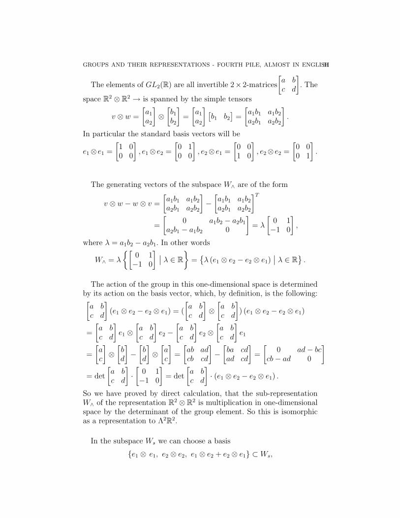
The elements of GL2(R) are all invertible 2× 2-matrices

[a bc d

]. The

space R2 ⊗ R2 → is spanned by the simple tensors

v ⊗ w =

[a1

a2

]⊗[b1

b2

]=

[a1

a2

] [b1 b2

]=

[a1b1 a1b2

a2b1 a2b2

].

In particular the standard basis vectors will be

e1⊗ e1 =

[1 00 0

], e1⊗ e2 =

[0 10 0

], e2⊗ e1 =

[0 01 0

], e2⊗ e2 =

[0 00 1

].

The generating vectors of the subspace W∧ are of the form

v ⊗ w − w ⊗ v =

[a1b1 a1b2

a2b1 a2b2

]−[a1b1 a1b2

a2b1 a2b2

]T=

[0 a1b2 − a2b1

a2b1 − a1b2 0

]= λ

[0 1−1 0

],

where λ = a1b2 − a2b1. In other words

W∧ = λ

{[0 1−1 0

] ∣∣ λ ∈ R}

={λ (e1 ⊗ e2 − e2 ⊗ e1)

∣∣ λ ∈ R}.

The action of the group in this one-dimensional space is determinedby its action on the basis vector, which, by definition, is the following:[a bc d

](e1 ⊗ e2 − e2 ⊗ e1) = (

[a bc d

]⊗[a bc d

]) (e1 ⊗ e2 − e2 ⊗ e1)

=

[a bc d

]e1 ⊗

[a bc d

]e2 −

[a bc d

]e2 ⊗

[a bc d

]e1

=

[ac

]⊗[bd

]−[bd

]⊗[ac

]=

[ab adcb cd

]−[ba cdad cd

]=

[0 ad− bc

cb− ad 0

]= det

[a bc d

]·[

0 1−1 0

]= det

[a bc d

]· (e1 ⊗ e2 − e2 ⊗ e1) .

So we have proved by direct calculation, that the sub-representationW∧ of the representation R2 ⊗ R2 is multiplication in one-dimensionalspace by the determinant of the group element. So this is isomorphicas a representation to Λ2R2.

In the subspace Ws we can choose a basis

{e1 ⊗ e1, e2 ⊗ e2, e1 ⊗ e2 + e2 ⊗ e1} ⊂ Ws,

32 KAREN E. SMITH

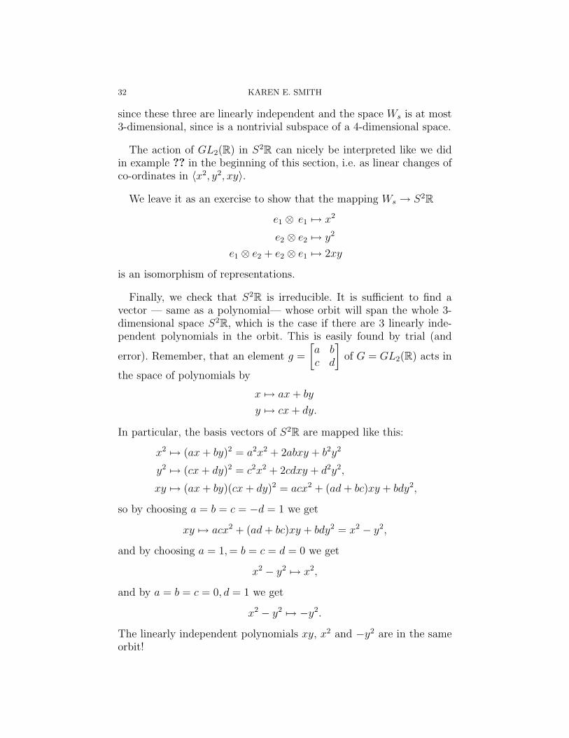
since these three are linearly independent and the space Ws is at most3-dimensional, since is a nontrivial subspace of a 4-dimensional space.

The action of GL2(R) in S2R can nicely be interpreted like we didin example ?? in the beginning of this section, i.e. as linear changes ofco-ordinates in 〈x2, y2, xy〉.

We leave it as an exercise to show that the mapping Ws → S2R

e1 ⊗ e1 7→ x2

e2 ⊗ e2 7→ y2

e1 ⊗ e2 + e2 ⊗ e1 7→ 2xy

is an isomorphism of representations.

Finally, we check that S2R is irreducible. It is sufficient to find avector — same as a polynomial— whose orbit will span the whole 3-dimensional space S2R, which is the case if there are 3 linearly inde-pendent polynomials in the orbit. This is easily found by trial (and

error). Remember, that an element g =

[a bc d

]of G = GL2(R) acts in

the space of polynomials by

x 7→ ax+ by

y 7→ cx+ dy.

In particular, the basis vectors of S2R are mapped like this:

x2 7→ (ax+ by)2 = a2x2 + 2abxy + b2y2

y2 7→ (cx+ dy)2 = c2x2 + 2cdxy + d2y2,

xy 7→ (ax+ by)(cx+ dy)2 = acx2 + (ad+ bc)xy + bdy2,

so by choosing a = b = c = −d = 1 we get

xy 7→ acx2 + (ad+ bc)xy + bdy2 = x2 − y2,

and by choosing a = 1,= b = c = d = 0 we get

x2 − y2 7→ x2,

and by a = b = c = 0, d = 1 we get

x2 − y2 7→ −y2.

The linearly independent polynomials xy, x2 and −y2 are in the sameorbit!


Now we have reduced the tensor product R2 ⊗ R2 to a direct sumwhich up to isomorphism is

R2 ⊗R2 = Λ2R⊕ S2R.

This result can be generalised to higher tensor powers, which we willdo later in ??.

28. Lie algebras — introduction

28.1. An abstract definition.

Definition 28.1. A lie algebra is a vector space V together with analternating bilinear mapping, called the lie bracket

V × V → V : (X, Y ) 7→ [X, Y ],

satisfying the Jacobi identity : for all X, Y, Z ∈ V :

[X, [Y, Z]] + [Y, [Z,X]] + [Z, [X, Y ]] = 0.

The coefficient field of the vector space F can be any field, but in thistext it is most often R, sometimes C.

A lie algebra homomorphism is a liner mapping f : V → V ′, whe-re V and V ′are lie algebras and f preserves brackets, in other words[f(X), f(Y )] = [X, Y ] for all X, Y ∈ V . A lien algebra isomorphism isalso a bijection, and its inverse will be a homomorphism.

A lie sub-algebra is a vector subspace of a lie algebra which is stableunder the bracket operation, i.e. ,it contains the brackets of its elements,so it is a lie algebra in its own right.

Remark 28.2. 1) Lie algebras form a category, in particular composedmappings of homomorphisms are homomorphisms.

2) A lie algebra is generally not associative. The Jacobi identity canbe seen as a surrogate property.

3) The motivation to consider lie algebras in the context of Lie groupsis the following: To each Lie group one can — in a natural way —associate a lie algebra, and essentially all lie algebras arise in this way.The same is true with respect to representations.

Example 28.3. The most trivial example of a lie algebra is the is triviallie algebra, i.e. any vector space with the zero bracket: [X, Y ] = 0

34 KAREN E. SMITH

Example 28.4. The fundamental example of a lie algebra is the spaceof all (invertible or not!) n× n-matrices

gln = gln(R) = Rn×n

equipped with the standard bracket

[X, Y ] = XY − Y X.It is easy to check that the standard bracket is an alternating bilinearmapping. The Jacobi identity is trivial as well: :

[X, Y Z − ZY ] + [Y, ZX −XZ] + [Z,XY − Y X]

= X(Y Z − ZY )− (Y Z − ZY )X + Y (ZX −XZ)

− (ZX −XZ)Y + Z(XY − Y X)− (XY − Y X)Z

= X(Y Z)− (XZ)Y − (Y Z)X + (ZY )X + Y (ZX)− Y (XZ)

− (ZX)Y + (XZ)Y + Z(XY )− Z(Y X)− (XY )Z + (Y X)Z

= XY Z −XZY − Y ZX + ZY X + Y ZX − Y XZ− ZXY +XZY + ZXY − ZY X −XY Z + Y XZ

= 0.

It will turn out that all lie algebras of finite dimensional lie groups aresub-algebras of this.

Example 28.5. The former ca be generalised. starting with any as-sociative algebra, U one can equip it with the usual bracket

[X, Y ] = XY − Y X.

Example 28.6. The following example of a lie algebra is also anexample of the lie algebra of a Lie group, and also an example of asub-lie-algebra of gln(R). Recall ?? that the tangent space of the Liegroup SLn(R) at the neutral element is s

Te(SLn(R)) = sln(R) = {X ∈ gln(R)∣∣ Tr(x) = 0}.

This is a lie sub-algebra, which can be checked by noticing that isis a vector subspace and [X, Y ] ∈ sln(R) whenever X, Y ∈ sln(R),something that must be proved by a little calculation — left to thereader.

Example 28.7. The Heisenberg lie algebra is a three dimensional vec-tor space V , where the brackets of the bais vectors are jossa kantavek-torien Lien sulkeet ovat

[X, Y ] = Z

[Y, Z] = 0

[Z,X] = 0.


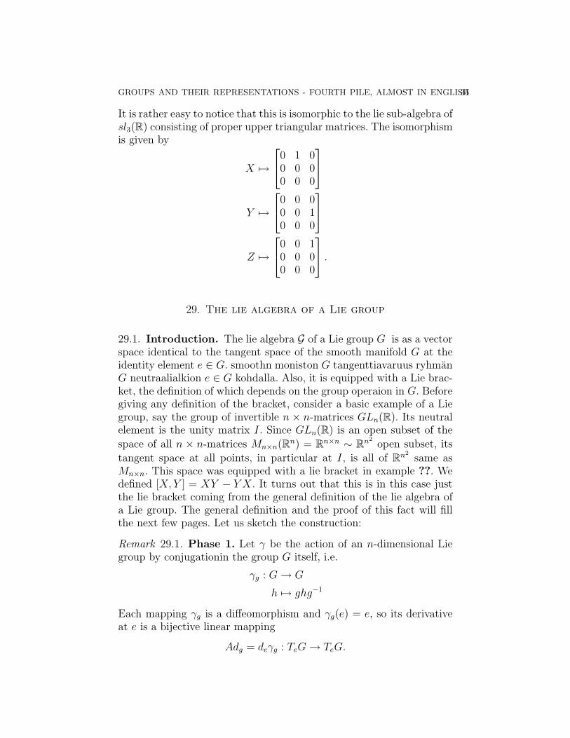
It is rather easy to notice that this is isomorphic to the lie sub-algebra ofsl3(R) consisting of proper upper triangular matrices. The isomorphismis given by

X 7→

0 1 00 0 00 0 0

Y 7→

0 0 00 0 10 0 0

Z 7→

0 0 10 0 00 0 0

.

29. The lie algebra of a Lie group

29.1. Introduction. The lie algebra G of a Lie group G is as a vectorspace identical to the tangent space of the smooth manifold G at theidentity element e ∈ G. smoothn moniston G tangenttiavaruus ryhmanG neutraalialkion e ∈ G kohdalla. Also, it is equipped with a Lie brac-ket, the definition of which depends on the group operaion in G. Beforegiving any definition of the bracket, consider a basic example of a Liegroup, say the group of invertible n × n-matrices GLn(R). Its neutralelement is the unity matrix I. Since GLn(R) is an open subset of the

space of all n × n-matrices Mn×n(Rn) = Rn×n ∼ Rn2open subset, its

tangent space at all points, in particular at I, is all of Rn2same as

Mn×n. This space was equipped with a lie bracket in example ??. Wedefined [X, Y ] = XY − Y X. It turns out that this is in this case justthe lie bracket coming from the general definition of the lie algebra ofa Lie group. The general definition and the proof of this fact will fillthe next few pages. Let us sketch the construction:

Remark 29.1. Phase 1. Let γ be the action of an n-dimensional Liegroup by conjugationin the group G itself, i.e.

γg : G→ G

h 7→ ghg−1

Each mapping γg is a diffeomorphism and γg(e) = e, so its derivativeat e is a bijective linear mapping

Adg = deγg : TeG→ TeG.

36 KAREN E. SMITH

In this way we have constructed a representation of the Lie group G inits own tangent space:

Ad : G→ GL(TeG) ∼ GLn(R)

g 7→ (Adg : TeG→ TeG)

Phase 2. We notice that also the mapping Ad is smooth. So it hasa derivative at e ∈ G. Define

ad = de(Ad) : TeG→ TI(GL(TeG))

X 7→ (adX : TeG→ TeG).

The derivative ad of the mapping Ad is a linear mapping from the tan-gent space TeG of G to the tangent space of the vector space GL(TeG)at I, which of course is the linear space itself

TI(GL(TeG)) ∼Mn×n ∼ {lineaarikuvaukset TeG→ TeG}.

Phase 3. Finally, define the lie bracket in TeG by

[X, Y ] = adXY.

It turns out that this mapping is a lie bracket in the abstract sense:bilinear, alternating and satisfying the Jacobi identity. We call the tan-gent space TeG with this bracket the lie algebra G of the Lie groupG.

Remark 29.2. It will take a while until we have proven all these state-ments. Let us begin by proving the existence and bilinearity of the liebracket in the tangent plane.

Phase1. Conjugation in a Lie group G is composed of two diffeo-morphisms,

γg : h 7→ gh 7→ g−1,

therefore itself a diffeomorphism, so its derivative

Adg = deγg : TeG→ TeG

at e exists and is a linear bijection. By the chain rule Adgg′ = deγgg′ =de(γg ◦ γg′) = dγ′(e)γg ◦ deγg′ = deγg ◦ deγg′ = AdgAdg′ , so we get arepresentation

Ad : G→ GL(TeG) ∼ GLn(R).

To be a Lie group representation, Ad has to be smooth. This may bedifficult to verify without using co-ordiantes, but a minute’s thoughtwill reveal that in local co-ordinates all components of the conjugationmapping G×G→ G : (g, h) 7→ ghg−1 are smooth real valued functions.Its derivative, which is nothing but Adg has a Jacobi matrix whose all


entries are partial derivatives of these components, hence smooth aswell. So the mapping g 7→ MatAdg is smooth i.e. Ad is smooth.

Phase 2. Adg has a derivative at e ∈ G, called ad. This derivativeis, by definition, a linear mapping, i.e.

TeG→ TI(GL(TeG)) ∼Mn×n ∼ {linear mappingsTeG→ TeG}.

Vaihe 3. a) Bilinearity: Since adX is a linear mapping TeG→ TeG,the mapping Y 7→ [X, Y ] = adXY is tof course linear in the variableY . Linearity in X depends on the fact that the mapping ad : X 7→ adXis the derivative of Ad, so it is linear.

We will only later (in ??) prove the rest, namely that our bracket is:

b) alternating and

c) satisfies the Jacobi identity

Instead of giving a proof, we inspect some examples::

Example 29.3. The Lie group S1 can be identified with the unit circleU(1) = {z ∈ C

∣∣ |z| = 1} ⊂ C ∼ R2, where multiplication of complexnumbers is the group operation and 1 is the neutral element. Conjuga-tion by the number g ∈ U(1) is nothing but z 7→ gzg−1 = zgg−1 = g,in other words every γg is the identical mapping. The derivative of theidentical mapping is of course the identical mapping of the tangentspace, so Ad is a constant mapping S1 → GL(T1S

1). The derivativeof a constant is zero, so adX = 0 for all X ∈ T1S

1 and consequently[X, Y ] = adXY = 0 for all X and Y .

The same argument shows that the lie algebra of every abelian Liegroup is trivial.

Example 29.4. Next we prove that the lie algebra of G = GLn(R)iswhat we dafined already in ?? namely gln(R). We alrady know thatthe tangent space of the manifold GLn(R) at the neutral element I isthe correct set TI(GLn(R)) = Rn×n. What remains to be proven is thatthe lie bracket defined by conjugation and the derivatives Ad and adwill be the same thing as the standard bracket in gln(R).

Conjugation by a matrix g is the mapping γg : h 7→ gh 7→ ghg−1,which is the composition of two linear mappings, hence linear, strictlyspeaking the restriction of a linear mapping Rn2 → Rn2

to the open

38 KAREN E. SMITH

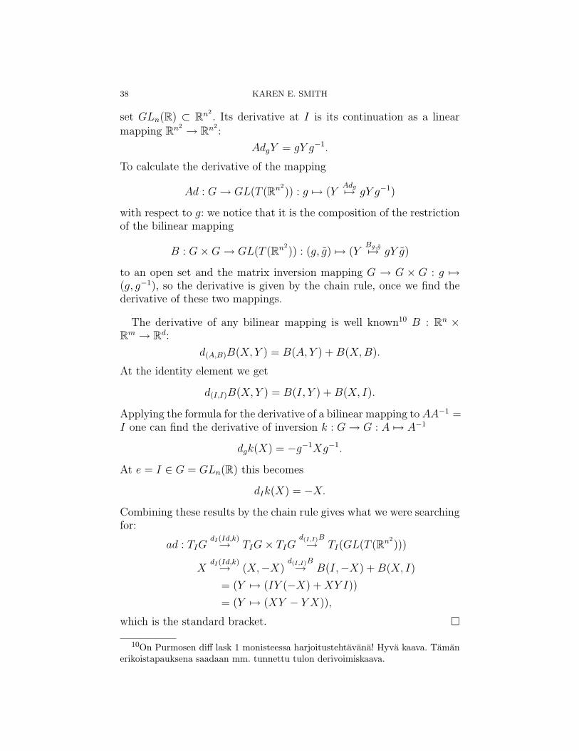
set GLn(R) ⊂ Rn2. Its derivative at I is its continuation as a linear

mapping Rn2 → Rn2:

AdgY = gY g−1.

To calculate the derivative of the mapping

Ad : G→ GL(T (Rn2

)) : g 7→ (YAdg7→ gY g−1)

with respect to g: we notice that it is the composition of the restrictionof the bilinear mapping

B : G×G→ GL(T (Rn2

)) : (g, g) 7→ (YBg,g7→ gY g)

to an open set and the matrix inversion mapping G → G × G : g 7→(g, g−1), so the derivative is given by the chain rule, once we find thederivative of these two mappings.

The derivative of any bilinear mapping is well known10 B : Rn ×Rm → Rd:

d(A,B)B(X, Y ) = B(A, Y ) +B(X,B).

At the identity element we get

d(I,I)B(X, Y ) = B(I, Y ) +B(X, I).

Applying the formula for the derivative of a bilinear mapping toAA−1 =I one can find the derivative of inversion k : G→ G : A 7→ A−1

dgk(X) = −g−1Xg−1.

At e = I ∈ G = GLn(R) this becomes

dIk(X) = −X.

Combining these results by the chain rule gives what we were searchingfor:

ad : TIGdI(Id,k)→ TIG× TIG

d(I,I)B→ TI(GL(T (Rn2

)))

XdI(Id,k)→ (X,−X)

d(I,I)B→ B(I,−X) +B(X, I)

= (Y 7→ (IY (−X) +XY I))

= (Y 7→ (XY − Y X)),

which is the standard bracket. �

10On Purmosen diff lask 1 monisteessa harjoitustehtavana! Hyva kaava. Tamanerikoistapauksena saadaan mm. tunnettu tulon derivoimiskaava.


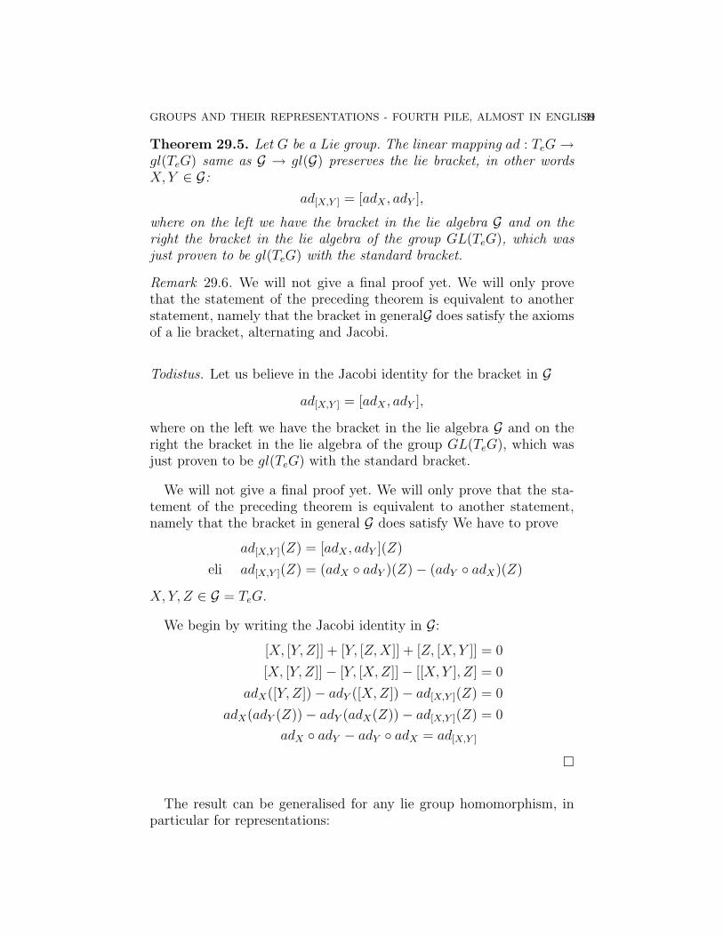
Theorem 29.5. Let G be a Lie group. The linear mapping ad : TeG→gl(TeG) same as G → gl(G) preserves the lie bracket, in other wordsX, Y ∈ G:

ad[X,Y ] = [adX , adY ],

where on the left we have the bracket in the lie algebra G and on theright the bracket in the lie algebra of the group GL(TeG), which wasjust proven to be gl(TeG) with the standard bracket.

Remark 29.6. We will not give a final proof yet. We will only provethat the statement of the preceding theorem is equivalent to anotherstatement, namely that the bracket in generalG does satisfy the axiomsof a lie bracket, alternating and Jacobi.

Todistus. Let us believe in the Jacobi identity for the bracket in G

ad[X,Y ] = [adX , adY ],

where on the left we have the bracket in the lie algebra G and on theright the bracket in the lie algebra of the group GL(TeG), which wasjust proven to be gl(TeG) with the standard bracket.

We will not give a final proof yet. We will only prove that the sta-tement of the preceding theorem is equivalent to another statement,namely that the bracket in general G does satisfy We have to prove

ad[X,Y ](Z) = [adX , adY ](Z)

eli ad[X,Y ](Z) = (adX ◦ adY )(Z)− (adY ◦ adX)(Z)

X, Y, Z ∈ G = TeG.

We begin by writing the Jacobi identity in G:

[X, [Y, Z]] + [Y, [Z,X]] + [Z, [X, Y ]] = 0

[X, [Y, Z]]− [Y, [X,Z]]− [[X, Y ], Z] = 0

adX([Y, Z])− adY ([X,Z])− ad[X,Y ](Z) = 0

adX(adY (Z))− adY (adX(Z))− ad[X,Y ](Z) = 0

adX ◦ adY − adY ◦ adX = ad[X,Y ]

�

The result can be generalised for any lie group homomorphism, inparticular for representations:

40 KAREN E. SMITH

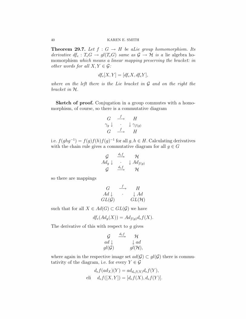
Theorem 29.7. Let f : G → H be aLie group homomorphism. Itsderivative dfe : TeG → gl(TeG) same as G → H is a lie algebra ho-momorphism which means a linear mapping preserving the bracket: inother words for all X, Y ∈ G:

dfe[X, Y ] = [dfeX, dfeY ],

where on the left there is the Lie bracket in G and on the right thebracket in H.

Sketch of proof. Conjugation in a group commutes with a homo-morphism, of course, so there is a commutative diagram

Gf−→ H

γg ↓ · ↓ γf(g)

Gf−→ H

i.e. f(ghg−1) = f(g)f(h)f(g)−1 for all g, h ∈ H. Calculating derivativeswith the chain rule gives a commutative diagram for all g ∈ G

G def−→ HAdg ↓ · ↓ Adf(g)

G def−→ H

so there are mappings

Gf−→ H

Ad ↓ · ↓ AdGL(G) GL(H)

such that for all X ∈ Ad(G) ⊂ GL(G) we have

dfe(Adg(X)) = Adf(g)def(X).

The derivative of this with respect to g gives

G def−→ Had ↓ ↓ adgl(G) gl(H),

where again in the respective image set ad(G) ⊂ gl(G) there is commu-tativity of the diagram, i.e. for every Y ∈ G

def(adX)(Y ) = addef(X)def(Y ),

eli def([X, Y ]) = [def(X), def(Y )].


30. The exponential mapping — a preliminary definition

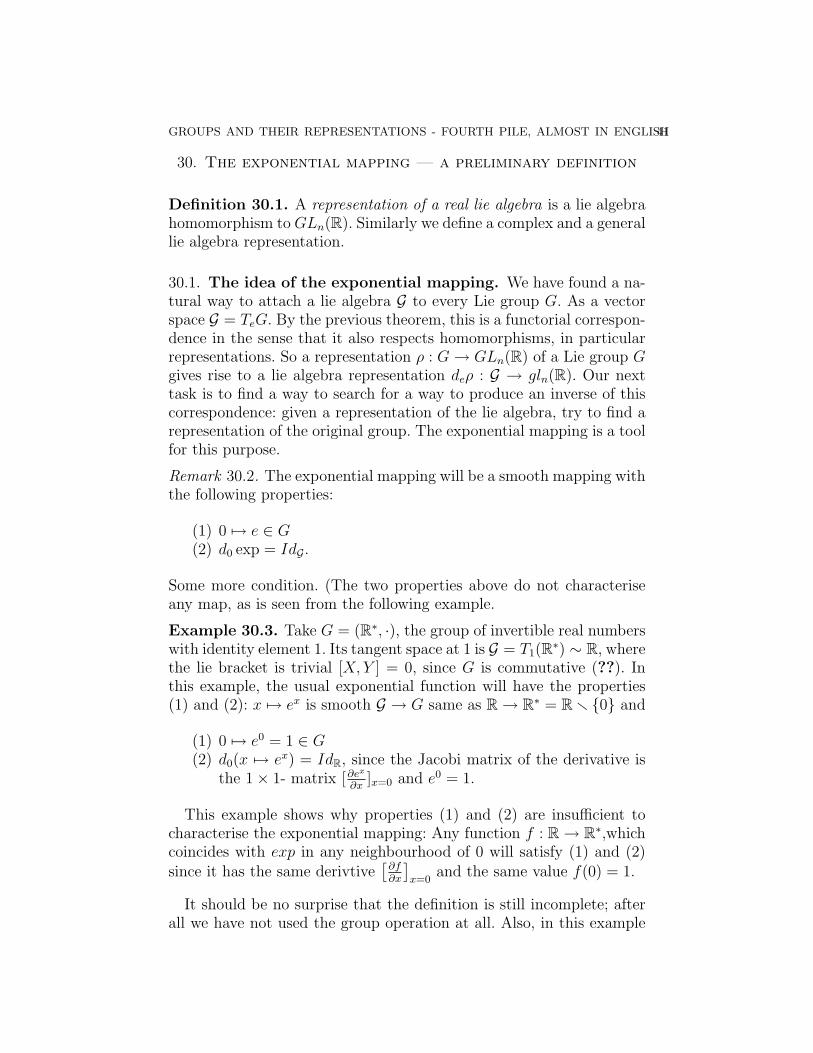
Definition 30.1. A representation of a real lie algebra is a lie algebrahomomorphism to GLn(R). Similarly we define a complex and a generallie algebra representation.

30.1. The idea of the exponential mapping. We have found a na-tural way to attach a lie algebra G to every Lie group G. As a vectorspace G = TeG. By the previous theorem, this is a functorial correspon-dence in the sense that it also respects homomorphisms, in particularrepresentations. So a representation ρ : G→ GLn(R) of a Lie group Ggives rise to a lie algebra representation deρ : G → gln(R). Our nexttask is to find a way to search for a way to produce an inverse of thiscorrespondence: given a representation of the lie algebra, try to find arepresentation of the original group. The exponential mapping is a toolfor this purpose.

Remark 30.2. The exponential mapping will be a smooth mapping withthe following properties:

(1) 0 7→ e ∈ G(2) d0 exp = IdG.

Some more condition. (The two properties above do not characteriseany map, as is seen from the following example.

Example 30.3. Take G = (R∗, ·), the group of invertible real numberswith identity element 1. Its tangent space at 1 is G = T1(R∗) ∼ R, wherethe lie bracket is trivial [X, Y ] = 0, since G is commutative (??). Inthis example, the usual exponential function will have the properties(1) and (2): x 7→ ex is smooth G → G same as R→ R∗ = R r {0} and

(1) 0 7→ e0 = 1 ∈ G(2) d0(x 7→ ex) = IdR, since the Jacobi matrix of the derivative is

the 1× 1- matrix [∂ex

∂x]x=0 and e0 = 1.

This example shows why properties (1) and (2) are insufficient tocharacterise the exponential mapping: Any function f : R→ R∗,whichcoincides with exp in any neighbourhood of 0 will satisfy (1) and (2)since it has the same derivtive

[∂f∂x

]x=0

and the same value f(0) = 1.

It should be no surprise that the definition is still incomplete; afterall we have not used the group operation at all. Also, in this example

42 KAREN E. SMITH

it happens tha exp happens to be a group homomorphism from theadditive group of the vector space to the group G but this is not truefor a general exponential map of a Lie group. It is just a consequenceof this example happening to be one dimensional.

Next we define the exponential mapping for all ”classical” Lie groups/algebras.

Definition 30.4. The classical exponential mapping is the mapping

exp : Mn×n →Mn×n

A 7→∞∑p=0

1

p!Ap = I + A+

1

2AA+

1

6AAA+ · · ·

It is easy to verify the absolute convergence of this series in the usualEuclidean topology of Mn×n = Rn×n. One can do it by using the wellknown matrix norm ‖A‖M = {sup ‖Ax‖

∣∣ ‖x‖ ≤ 1} or by estimatingthe Euclidean norm using the inequalities

‖A‖ ≤ n2 maxi,j|Aij|

and

[Ap]ij ≤ (n ·maxi,j|Aij|)p.

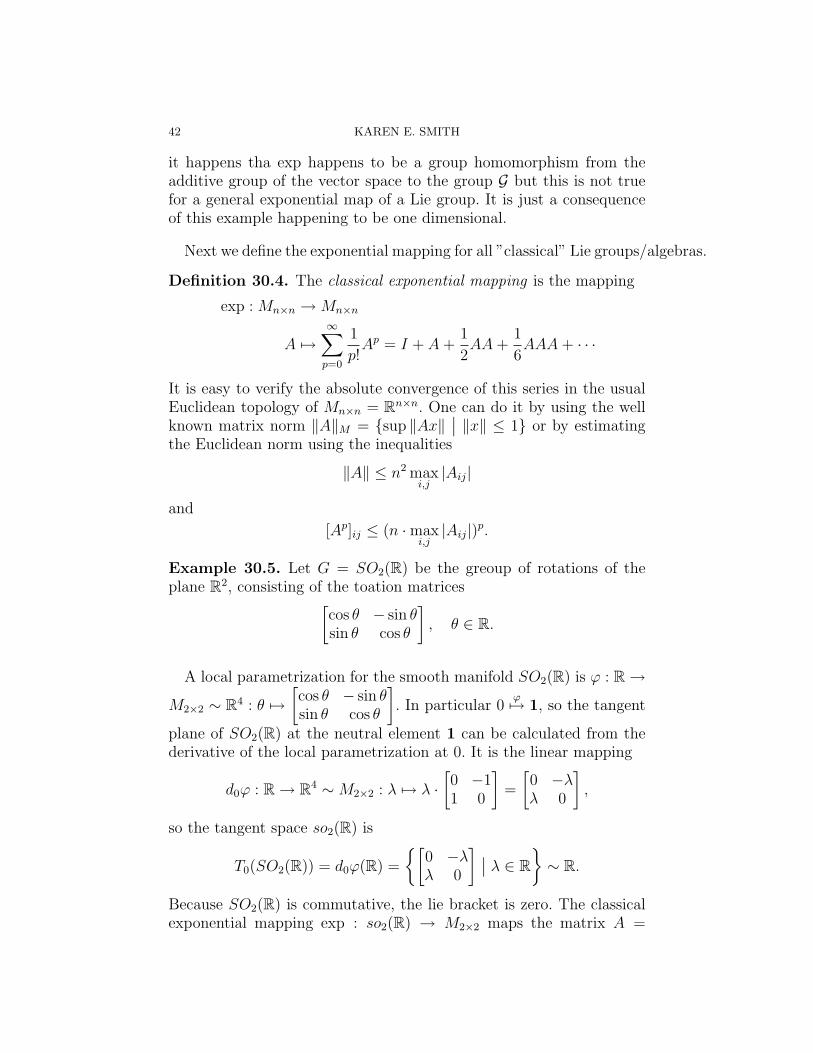
Example 30.5. Let G = SO2(R) be the greoup of rotations of theplane R2, consisting of the toation matrices[

cos θ − sin θsin θ cos θ

], θ ∈ R.

A local parametrization for the smooth manifold SO2(R) is ϕ : R→

M2×2 ∼ R4 : θ 7→[cos θ − sin θsin θ cos θ

]. In particular 0

ϕ7→ 1, so the tangent

plane of SO2(R) at the neutral element 1 can be calculated from thederivative of the local parametrization at 0. It is the linear mapping

d0ϕ : R→ R4 ∼M2×2 : λ 7→ λ ·[0 −11 0

]=

[0 −λλ 0

],

so the tangent space so2(R) is

T0(SO2(R)) = d0ϕ(R) =

{[0 −λλ 0

] ∣∣ λ ∈ R}∼ R.

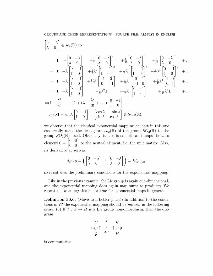
Because SO2(R) is commutative, the lie bracket is zero. The classicalexponential mapping exp : so2(R) → M2×2 maps the matrix A =

GROUPS AND THEIR REPRESENTATIONS - FOURTH PILE, ALMOST IN ENGLISH43[0 −λλ 0

]∈ so2(R) to

1 +

[0 −λλ 0

]+1

2

[0 −λλ 0

]2

+ 13!

[0 −λλ 0

]3

+ 14!

[0 −λλ 0

]4

+ . . .

= 1 +λ

[0 −11 0

]+1

2λ2

[0 −11 0

]2

+ 13!λ3

[0 −11 0

]3

+ 14!λ4

[0 −11 0

]4

+ . . .

= 1 +λ

[0 −11 0

]+1

2λ2

[−1 00 −1

]+ 1

3!λ3

[0 1−1 0

]+ 1

4!λ4

[1 00 1

]+ . . .

= 1 +λ

[0 −11 0

]−1

2λ21 − 1

3!λ3

[0 −11 0

]+ 1

4!λ41 + . . .

=(1− λ3

3!+ . . . )1 + (λ− λ2

2!+ . . . )

[0 −11 0

]= cosλ1 + sinλ

[0 −11 0

]=

[cosλ − sinλsinλ cosλ

]∈ SO2(R).

we observe that the classical exponential mapping at least in this onecase really maps the lie algebra so2(R) of the group SO2(R) to thegroup SO2(R) itself. Obviously, it also is smooth and maps the zero

element 0 =

[0 00 0

]to the neutral element, i.e. the unit matrix. Also,

its derivative at zero is

d0exp =

([0 −λλ 0

]7→[

0 −λλ 0

])= Idso2(R),

so it satisfies the preliminary conditions for the exponential mapping.

Like in the previous example, the Lie group is again one-dimensional,and the exponential mapping does again map sums to products. Werepeat the warning: this is not true for exponential maps in general.

Definition 30.6. (Move to a better place!) In addition to the condi-tions in ?? the exponential mapping should be natural in the followingsense: (3) If f : G → H is a Lie group homomorphism, then the dia-gram

Gf→ H

exp ↑ · ↑ exp

G def→ H

is commutative

44 KAREN E. SMITH

31. Vector fields on manifolds

31.1. Introduction. Every homomorphism of a Lie group ρ : G →H, in particular every representation, has a derivative at the neutralelement, and this derivative d0ρ : G → G is a homomorphism of liealgebras. In fact every lie algebra homomorphism is the derivative ofsome Lie group homomorphism:

If G is a ”concrete” Lie group, same as aa sub-Lie group of GLn(R), then the classical exponential mapping is a mapping G → G, and ifT : G → G is a homomorphism of lie algebras, then there exists a Liegroup homomorphism ρ : G→ H such, that T = d0ρ. Since Euclideanspace G is connected, its continuous image exp(G) ⊂ G is connected aswell. Therefore the image of the exponential mapping is contained inthe connected component of the Lie group which contains the neutralelement. It turns out that ifG happens to be simply connected, then theclassical exponential mapping will define a 1-1-correspondence betweenrepresentations of the Lie group G and its lie algebra G.

The following Lie groups are simply connected:

(1) {M ∈ GLn(R)∣∣M is upper diagonal with all diagonal elements

equal to 1.}.(2) closed Lie subgroups of the above(3) the neutral element’s connected component in a ny Lie group.(4) the universal covering group of any Lie group. By this we mean

the following: Talla tarkoitetaan seuraavaa: Every manifold Mhas a unique universal covering space whgich is a manifold Ptogether with a smooth surjection, the covering map π : P →Msuch, that every x ∈M has a neighbourhood U , whose preimageπ1(U) consists of a collection of distinct sets each diffeomorphicto U :

U =⋃i∈I

Ui π∣∣Ui

: Ui → U is a diffeomorphism.

The universal covering space of a Lie group can be given thestructure of a Lie group such that π becomes a homomorp-hism.11.

It is obvious that a Lie group and its universal covering grouphave the same lie algebra.

11OK?


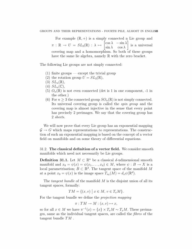
For example (R,+) is a simply connected n Lie group and

π : R → U = SL2(R) : λ 7→[cosλ − sinλsinλ cosλ

]is a universal

covering map and a homomorphism. So both of these groupshave the same lie algebra, namely R with the zero bracket.

The following Lie groups are not simply connected:

(1) finite groups — except the trivial group(2) the rotation group U = SL2(R),(3) SLn(R),(4) SLn(C),(5) On(R) is not even connected (det is 1 in one component, -1 in

the other.)(6) For n ≥ 3 the connected group SOn(R) is not simply connected.

Its universal covering group is called the spin group and thecovering map is almost injective in the sense that every pointhas precisely 2 preimages. We say that the covering group has2 sheets.

We will now prove that every Lie group has an exponential mappingG → G which maps representations to representations. The construc-tion of such an exponential mapping is based on the concept of a vectorfield on manifolds and on some theory of differential equations.

31.2. The classical definition of a vector field. We consider smoothmanifolds which need not necessarily be Lie groups.

Definition 31.1. Let M ⊂ Rn be a classical d-udimensional smoothmanifold and x0 = ψ(x) = ψ(x1, . . . , xd) ∈ M , where ψ : B → X is alocal parametrisation; B ⊂ Rd. The tangent space of the manifold Mat a point x0 = ψ(x) is the image space Tx0(M) = dxψ(Rd).

The tangent bundle of the manifold M is the disjoint union of all itstangent spaces, formally:

TM = {(x, v)∣∣ x ∈M, v ∈ TxM}.

For the tangent bundle we define the projection mapping

π : TM →M : (x, v) 7→ x,

so for all x ∈M we have π−1(x) = {x} × TxM ∼ TxM . These preima-ges, same as the individual tangent spaces, are called the fibres of thetangent bundle TM .

46 KAREN E. SMITH

The tangent bundle is also equipped with the structure of a smoothmanifold. This is done by taking the local trivialisations

ϕT : π−1(U)→ ϕ(U)× Rd

(x, v) 7→ (ϕ(x), dxϕv),

as charts where the ϕ : U → B ⊂ Rd are the charts of the originalmanifold M .

PICTURE TO BE DRAWN LATER

Kuva 999: tangenttikimpun lokaali trivialisointi

Example 31.2. The tangent bundle of the circle M = S1 is the cylin-der S1 ×R with the structure of the product manifold and the projec-tion map π : S1×R→ S1 : (x, u) 7→ x. A tangent bundle isomorphic toM ×Rd is called a trivial tangent bundle. so the tangent bundle of thecircle is trivial but we will soon notice that the tangent bundle of thetwo dimensional sphere is not. On the other hand, the tangent bundleof every Lie group is trivial.

Definition 31.3. A vector field on a manifold M is a smooth mappingX : M → TM , such that π ◦ X = IdM or equivalently ∀x ∈ M :X(x) ∈ {x} × TxM .

Proposition 31.4. ”You cannot comb the hair on a sphere —theorem”12 Every vector field on the 2-dimensional sphere S2 = {x ∈R3∣∣ ‖x‖ = 1} has a zero point.

Todistus. The proof would lead us too much astray. Consult the litera-ture. �

Corollary 31.5. The tangent bundle TS2 of the sphere S2 has no glo-bal frame by which we mean such a pair of vector fields X1, X2, thatX1(x), X2(x) would be a basis for the tangent space TxS2 at each x ∈ S2.

12There are nice videos on Youtube, where this is tried!


Corollary 31.6. The tangent bundle TS2 of the sphere S2 has noglobal trivialisation by which we mean a diffeomorphism f : TS2 →S2 × R2, with π ◦ f = f ◦ π.

Todistus. It is left as an exercise to prove that the tangent bundle ofa manifold has a global trivialisation if and only if it has a globalframe. �

For example the tangent bundle of the circle S1 i.e. the cylinder isgobally trivial but the manifold S1 has no atlas consisting of one chartonly.

(CORRECT THE FINNISH TEXT!)

31.3. Left invariant vector fields on a Lie group.

Definition 31.7. A vector field X on a Lie group ryhman G is leftinvariant, if for all g, h ∈ G

dx(mg)X(h) = X(gh),

where m : G→ G : h 7→ gh is multiplication from the left the elementg and dx(mg) : ThG→ TghG is its derivative.

Proposition 31.8. Let v ∈ TeG = G. Now

Xv; g 7→ (g, dx(mg)v)

is a left invariant vector field, where m : G → G : h 7→ gh is mul-tiplication from the left by the element g and dx(mg) : ThG→ TghG isits derivative.

Todistus. The mapping Xv is a vector field, since it is a compositionof smooth mappings, hence a smooth mapping X : M → TM andevidently X(x) ∈ {x} × TxM for all x ∈ M . Left invariance followsfrom the chain rule:

mgh : Gmh−→ G

mg−→ G| | |

demgh : TeGdemh−→ ThG

demg−→ TghG

.

�

If v 6= 0, the vector field Xv has no zeros, in particular it — of course— cannot be the zero vector field, so v 7→ Xv is a linear injection,

48 KAREN E. SMITH

in fact a bijection TeG →{left invariant vector fields of G}. By thisbijection we can carry over the lie algebra structure of TeG to {leftinvariant vector fields of G :}.

By this construction we have been able to identify a single tangentvector X ∈ TeG with a vector field: The correspondence is

X 7→ (g 7→ demgX).

Having carried over the vector space structure and the lie bracketfrom X ∈ TeG we have made the set of left invariant vector fieldsinto a lie algebra. It is worth while to notice that the vector spaceoperations coincide with the ”natural pointwise” operations on generalvector fields: if X(x) = (x, v) and Y (x) = (x,w), then (αX+βY )(x) =(x, αv + βw). This is so, because the derivative of left multiplicationmg is a linear isomorphism TeG → TgG. By this isomorphism, we can– of course — also transfer the basis of TeG to TeG to TmG or to {leftinvariant vector fields of G :}, so every Lie group has a global frame.

Remark 31.9. We transferred the lie bracket by the linear isomorphismTeG → TmG, but in fact it is possible, and common, to define a liebracket of vector fields on any manifold. It turns out that this is not inconflict with our definition: the lie algebra {left invariant vector fieldsof G :} is a sub lie algebra of {all vector fields on G} with the moregeneral lie bracket.

Let us also notice that the mapping

g 7→ (X 7→ demgX)

is a representation of G in the space of its own left invariant vectorfields which we now have completely identified with the lie algebra G.

This can be generalised: If a Lie group G acts as diffeomorphismson any manifold M , then G acts linearly in the space V KM of allvector fields over M which is a representation of G. The representationis defined by the following construction: Let X : M → TM : x 7→(x,X(x)) be a vector field and take g ∈ G. The vector field gX is themapping

y 7→ (y, dxmgX(x)),

where we have denoted the action of g ∈ G in M by g and x = g−1y.

31.4. The general definition of the exponential mapping. Sincenot all Lie groups are matrix groups, and some are matrix groups only


by cumbersome identifications, there is need to re-define the exponen-tial mapping in an abstract setting. exp should be a mapping from thelie algebra G of a general Lie group G to the Lie group G itself andhave the following properties:

(1) 0 7→ e(2) d0 exp = IdG : G → G = T0(G)(3) for all X ∈ G the restriction exp

∣∣RX is a group homomorphism

RX ∼ R→ G, in other words for all λ, µ ∈ R and X ∈ G

exp((λ+ µ)X) = exp(λX) · exp(µX).

Condition (3) is often expressed by saying that the restrictionexp∣∣RX is a one parameter subgroup ofG.

Proposition 31.10. there exists a unique mapping satisfying the con-ditions (1)-(3).

Todistus. we prove the proposition by giving a construction in twosteps:

(Step 1) Interprete the elements X of the lie algebra G as left inva-riant vector spaces on G. This was done above.

(Step 2) From the theory of differential equations, adopt the factthat any everywhere non-zero vector field has a flow consisting of itsintegral curves. Roughly this means that it is possible to start at anypoint p on the manifold and then ”follow the vectors” interpreted as”velocities” for some time. If it is possible to follow a given vector fieldeverywhere for a a given time, say time 1, this will create a smoothmap from the manifold to itself, and the procedure can be repeatedgenerating a flow that ”goes on forever”. Let us do this in detail:

Define an integral curve of a given vector field X in a neighbourhoodU of a given point p ∈ M to be a smooth curve γX : ] − ε, ε[→ M ,mapping 0 7→ p and having derivatives

dtγX : R→ Tp(M) : s 7→ (γ(t), sX(γ(t)),

in particular

′′1dtγ7→ X ∈ Tγ(t)

′′.

50 KAREN E. SMITH

Such an integral curve always exists and is unique on a small enoughinterval ] − ε, ε[, but for a general vector field the interval cannot bechosen to be large let alone all of R.13

Let us sketch the next step: In a Lie group integral curves of leftinvariant vector fields can be extended to all of R and becomes a grouphomomorphism γ : (R,+) → G. This is done by ”translating” in G.Before doing this, we use the result to finish the construction of theexponential mapping: We define it to be

exp : G → G : X 7→ γX(1).

We have to notice that this mapping obviously satisfies the conditions(1) . . . (3) and is, by uniqueness of the integral curves, the only mappingdoing so.

What is left of the construction is the promised extension of the in-tegral curve of a left invariant vector field. Let the integral curve bedefined on ] − ε, ε[- By uniqueness of the integral curves the ”homo-morphism formula” γX(s + t) = γX(s) · γX(t) holds at least for all|t| ≤ ε

2and |s| ≤ ε

2, since for fixed s both sides are, as functions of t,

integral curves of the same vector field X in the neighbourhood of thesame point γX(s). Let us verify this in detail:

Introduce some short hand notation: γ = γX , α(t) = γX(s + t)and β(t) = γX(s) · γX(t). Obviously both have the same initial valueα(0) = β(0) = γX(s). furthermore both are integral curves of the vectorfield X, since by the definition ?? of an integral curve

dtγ : R→ Tγ(t)(M) : r 7→ rX(γ(t))

which, expressed as a formula for the basis vector 1 of R is equivalentto:

dtγ : R→ Tγ(t)(M) : 1 7→ X(γ(t))

and gives for α:

dtα :R Id=dt(r 7→s+r)−→ R ds+t(γ)−→ Tα(t)G

1 7→ dt+s(γ) = X(γ(s+ t)) = X(α(t)).

and for β = mγ(s) ◦ γ:

dtβ :R dtγ−→ Tγ(t)(G)dγ(t)(mγ(s))−→ Tβ(t)(G)

1 7→ X(γ(t)) 7→ dγ(t)(mγ(s))(X(γ(t)))vas.inv!

= X(γ(s) · γ(t)) = X(β(t)).

13Counterexample: a constant vector field in an open circle ⊂ R2.


Define for all r ∈]− 2ε, 2ε[

γX(r) = γX( r2

+ r2) = γX( r

2) · γX( r

2).

We have already proved that this extension is not anywhere in conflictwith the original definition. Also, it should be clear (exercise?) that theextended curve γX is an integral curve of X with the same initial point.The continuation process can be repeated to find an integral curve γXdefined on ]− 2nε, 2nε[ and all in all in R.

�

Infinite Groups - Jyväskylän yliopistousers.jyu.fi/~laurikah/REP/REPtext2010_4E.pdf · Infinite...

Documents

Transcript of Infinite Groups - Jyväskylän yliopistousers.jyu.fi/~laurikah/REP/REPtext2010_4E.pdf · Infinite...