INFERENCE OF COMPUTATIONAL MODELS OF TENDON NETWORKS

VIA SPARSE EXPERIMENTATION

by

Manish Umesh Kurse

A Dissertation Presented to theFACULTY OF THE USC GRADUATE SCHOOLUNIVERSITY OF SOUTHERN CALIFORNIA

In Partial Fulfillment of theRequirements for the Degree

DOCTOR OF PHILOSOPHY(BIOMEDICAL ENGINEERING)

August 2012

Copyright 2012 Manish Umesh Kurse

Dedication

To my parents.

ii

Acknowledgements

Little did I know when I started my Ph.D. that this journey I was about to undertake

would teach me invaluable life lessons that would change my view of the world. I have

several people to thank for these lessons, whose roads crossed mine during these years.

Firstly, I would like to thank Dr. Francisco Valero-Cuevas for being a fantastic adviser

and mentor to me the last five and a half years. He has guided me, supported me and

helped me get an education that goes well beyond engineering. I have learnt from him the

importance of good presentation of ideas and how to communicate to a diverse audience.

By bringing together a team of very smart individuals from different academic and cultural

backgrounds, he gave me an opportunity to enrich myself, expand my thinking and along

the way make some great friends.

In spite of a three hour time zone difference and a busy schedule, Dr. Hod Lipson

was always available to meet with me for our teleconference meetings. Some of his ideas

form the core of my dissertation research. Working in his lab during Dec ’09-Jan ’10 at

Cornell University, though short, was a great experience and had significant impact on

my Ph.D.

I would like to thank Dr. Gerald Loeb and Dr. Eva Kanso for being on my dissertation

committee and for their honest comments and inputs which helped me question, rethink

iii

and reshape my approach to the problem I was trying to solve. I would like to thank Dr.

Terence Sanger for being on my dissertation guidance committee.

Dr. Jason Kutch taught me to question, think and innovate. I learned that with good

planning and sincere hard work any idea can be taken from concept to reality. I owe it

to him for training me in the art of experimentation.

Every Ph.D. has its ups and downs and I’ve had my fair share over the last few years.

Sudarshan has been a fantastic friend who has been by my side throughout this journey

to share the joys and frustrations of Ph.D. research. We started and finished our journeys

at USC around the same time and having him around definitely made the journey easier

and more fun. I have always admired his knowledge and view of the world that has

greatly influenced my own thinking.

Josh Inouye has been a great friend and a source of inspiration. His efficient working

style, getting things done attitude and discipline has motivated me to work harder and

be more productive. I have had good discussions with him about my research and his

feedback has always been very valuable.

Kornelius has been a good friend and a co-traveller in my journey from almost the

very beginning. Along with Sudarshan, we saw the growth of the lab from the very

scratch. Its been great working with him over the years.

Thanks to Brendan for helping me with computer hardware, graphics related issues

and making good videos. He has been a good friend, my tennis buddy and introduced

me to some great fiction.

Several people have been an integral part of the cadaver experiments: Heiko Hoffmann,

forming the ‘cadaver dream team’ with Jason and me; the hand surgeons: Dr. Vincent

iv

Hentz, Dr. Caroline Leclercq, Dr. Isabella Fassola and Dr. Nina Lightdale; and the Brain-

Body Dynamics Lab members and alumni : Dr. Marta Mora Aguilar, Emily Lawrence,

Srideep Musuvathy, John Rocamora and Hannah Ko. Thanks to Alex, Evangelos, for

their inputs to my research at various points in my PhD.

Mischalgrace Diasanta has been a great graduate student adviser and a fun collabo-

rator during my Biomedical Engineering Senator year.

Harsha, Kapish, Heeral, Tapan, Anish and Devanshi have become very close friends

with whom I have shared fun times over many dinners and card game nights. It is thanks

to them and the Veggie Hiker group that I fell in love with Los Angeles.

I would like to thank my dear parents who have been extremely supportive throughout

my education. I have shared with them my successes and my disappointments at every

stage in my life and they have always been encouraging and positive. Without their love

and support, I would not have been able to come this far. I also thank my grandmother

for her best wishes, love and affection.

v

Table of Contents

Dedication ii

Acknowledgements iii

List of Tables x

List of Figures xi

Abstract xiv

Chapter 1: Introduction 11.1 Background . . . . . . . . . . . . . . . . . . . . . . . . . . . . . . . . . . . 11.2 Modeling the Human Tendon Networks . . . . . . . . . . . . . . . . . . . 2

1.2.1 Anatomy . . . . . . . . . . . . . . . . . . . . . . . . . . . . . . . . 31.2.2 Functional Significance of the Extensor Mechanism . . . . . . . . . 3

1.3 Previous Work . . . . . . . . . . . . . . . . . . . . . . . . . . . . . . . . . 71.3.1 Prior Work in the Lab Leading to Current Work . . . . . . . . . . 10

1.4 Significance of Research . . . . . . . . . . . . . . . . . . . . . . . . . . . . 121.5 Dissertation Outline . . . . . . . . . . . . . . . . . . . . . . . . . . . . . . 13

1.5.1 Chapter 2 . . . . . . . . . . . . . . . . . . . . . . . . . . . . . . . . 131.5.2 Chapter 3 . . . . . . . . . . . . . . . . . . . . . . . . . . . . . . . . 131.5.3 Chapter 4 . . . . . . . . . . . . . . . . . . . . . . . . . . . . . . . . 141.5.4 Chapter 5 . . . . . . . . . . . . . . . . . . . . . . . . . . . . . . . . 141.5.5 Chapter 6 . . . . . . . . . . . . . . . . . . . . . . . . . . . . . . . . 151.5.6 Chapter 7 . . . . . . . . . . . . . . . . . . . . . . . . . . . . . . . . 151.5.7 Chapter 8 . . . . . . . . . . . . . . . . . . . . . . . . . . . . . . . . 151.5.8 Chapter 9 . . . . . . . . . . . . . . . . . . . . . . . . . . . . . . . . 151.5.9 Chapter 10 . . . . . . . . . . . . . . . . . . . . . . . . . . . . . . . 16

Chapter 2: Fundamentals of Biomechanical Modeling 172.1 Computational Environments . . . . . . . . . . . . . . . . . . . . . . . . . 182.2 Dimensionality and Redundancy . . . . . . . . . . . . . . . . . . . . . . . 202.3 Skeletal Mechanics . . . . . . . . . . . . . . . . . . . . . . . . . . . . . . . 222.4 Musculotendon Routing . . . . . . . . . . . . . . . . . . . . . . . . . . . . 242.5 Musculotendon Models . . . . . . . . . . . . . . . . . . . . . . . . . . . . . 26

vi

2.6 Forward and Inverse Simulations . . . . . . . . . . . . . . . . . . . . . . . 282.6.1 Forward Models . . . . . . . . . . . . . . . . . . . . . . . . . . . . 282.6.2 Inverse Models . . . . . . . . . . . . . . . . . . . . . . . . . . . . . 29

Chapter 3: Extrapolatable Analytical Functions for Tendon Excursionsand Moment Arms from Sparse Datasets 313.1 Abstract . . . . . . . . . . . . . . . . . . . . . . . . . . . . . . . . . . . . . 313.2 Introduction . . . . . . . . . . . . . . . . . . . . . . . . . . . . . . . . . . . 323.3 Methods . . . . . . . . . . . . . . . . . . . . . . . . . . . . . . . . . . . . . 37

3.3.1 Symbolic Regression Using Genetic Programming . . . . . . . . . . 373.3.2 Comparison Against Polynomial Regression . . . . . . . . . . . . . 393.3.3 Experimental Data from a Tendon-Driven Robotic System . . . . . 40

3.3.3.1 Reducing the Size of the Training Dataset . . . . . . . . . 413.3.3.2 Increasing the Range of Extrapolation . . . . . . . . . . . 42

3.3.4 Computer-Generated Synthetic Data . . . . . . . . . . . . . . . . . 423.3.4.1 Robustness to Noise . . . . . . . . . . . . . . . . . . . . . 453.3.4.2 Number of Free Parameters . . . . . . . . . . . . . . . . . 47

3.4 Results . . . . . . . . . . . . . . . . . . . . . . . . . . . . . . . . . . . . . . 473.4.1 Results for the Experimental Tendon-Driven Robotic System . . . 47

3.4.1.1 Effect of Reducing the Size of the Training dataset . . . . 473.4.1.2 Effect of Increasing the Range of Extrapolation . . . . . . 49

3.4.2 Results for the Computer-Generated Synthetic Data . . . . . . . . 523.4.2.1 Robustness to Noise . . . . . . . . . . . . . . . . . . . . . 523.4.2.2 Number of Free Parameters as a Practical Measure of the

Complexity of the Analytical Expression . . . . . . . . . 553.5 Discussion . . . . . . . . . . . . . . . . . . . . . . . . . . . . . . . . . . . . 55

Chapter 4: Simultaneous Inference of the Form and Parameters of Ana-lytical Models Describing Tendon Routing in the Human Fingers. 624.1 Abstract . . . . . . . . . . . . . . . . . . . . . . . . . . . . . . . . . . . . . 624.2 Introduction . . . . . . . . . . . . . . . . . . . . . . . . . . . . . . . . . . . 634.3 Methods . . . . . . . . . . . . . . . . . . . . . . . . . . . . . . . . . . . . . 65

4.3.1 Experimental Setup and Data Collection . . . . . . . . . . . . . . . 654.3.2 Symbolic Regression Implementation Using Eureqa . . . . . . . . . 674.3.3 Comparison Against Polynomial Regression and Landsmeer-Based

Models . . . . . . . . . . . . . . . . . . . . . . . . . . . . . . . . . 694.3.3.1 Two Movement Trials from the Same Cadaveric Specimen 704.3.3.2 Two Trials with Two Different Cadaveric Specimens . . . 70

4.4 Results . . . . . . . . . . . . . . . . . . . . . . . . . . . . . . . . . . . . . . 714.5 Discussion . . . . . . . . . . . . . . . . . . . . . . . . . . . . . . . . . . . . 75

Chapter 5: Experimental Cadaveric Actuation Gives Insight on Controlof Human Finger Movement 795.1 Abstract . . . . . . . . . . . . . . . . . . . . . . . . . . . . . . . . . . . . . 795.2 Introduction . . . . . . . . . . . . . . . . . . . . . . . . . . . . . . . . . . . 805.3 Methods . . . . . . . . . . . . . . . . . . . . . . . . . . . . . . . . . . . . . 81

vii

5.3.1 Control of Finger Tapping Motion . . . . . . . . . . . . . . . . . . 835.3.2 Finger Equilibrium Study . . . . . . . . . . . . . . . . . . . . . . . 83

5.4 Results . . . . . . . . . . . . . . . . . . . . . . . . . . . . . . . . . . . . . . 875.4.1 Results from Control of Finger Tapping Motion . . . . . . . . . . . 875.4.2 Results from Finger Equilibrium Study . . . . . . . . . . . . . . . 87

5.5 Discussion . . . . . . . . . . . . . . . . . . . . . . . . . . . . . . . . . . . . 905.6 Appendix: Mathematical Explanation of Finger Equilibria . . . . . . . . . 945.7 Appendix: A Strain-Energy Approach to Simulating Slow Finger Move-

ments and Changes Due to Loss of Musculature . . . . . . . . . . . . . . . 965.7.1 Introduction . . . . . . . . . . . . . . . . . . . . . . . . . . . . . . 965.7.2 Methods . . . . . . . . . . . . . . . . . . . . . . . . . . . . . . . . . 965.7.3 Results and Discussion . . . . . . . . . . . . . . . . . . . . . . . . . 100

Chapter 6: Experimental Validation of Existing Models of the Index Fin-ger 1016.1 Introduction . . . . . . . . . . . . . . . . . . . . . . . . . . . . . . . . . . . 1016.2 Methods . . . . . . . . . . . . . . . . . . . . . . . . . . . . . . . . . . . . . 1036.3 Results . . . . . . . . . . . . . . . . . . . . . . . . . . . . . . . . . . . . . . 1056.4 Discussion . . . . . . . . . . . . . . . . . . . . . . . . . . . . . . . . . . . . 107

Chapter 7: Study of the Sensitivity of Fingertip Force Output to Topol-ogy and Parameters of the Extensor Mechanism Using a Novel FiniteElement Analysis Simulator 1087.1 Abstract . . . . . . . . . . . . . . . . . . . . . . . . . . . . . . . . . . . . . 1087.2 Introduction . . . . . . . . . . . . . . . . . . . . . . . . . . . . . . . . . . . 1097.3 Methods . . . . . . . . . . . . . . . . . . . . . . . . . . . . . . . . . . . . . 111

7.3.1 The Tendon Network Simulator . . . . . . . . . . . . . . . . . . . . 1117.3.2 Experimental Validation of the Tendon Network Simulator . . . . 1137.3.3 Simulating the Extensor Mechanism . . . . . . . . . . . . . . . . . 1147.3.4 Sensitivity Analysis . . . . . . . . . . . . . . . . . . . . . . . . . . 116

7.4 Results . . . . . . . . . . . . . . . . . . . . . . . . . . . . . . . . . . . . . . 1187.4.1 Results of validation of the tendon network . . . . . . . . . . . . . 1187.4.2 Results of Sensitivity Analysis . . . . . . . . . . . . . . . . . . . . 118

7.5 Discussion . . . . . . . . . . . . . . . . . . . . . . . . . . . . . . . . . . . . 1217.6 Appendix . . . . . . . . . . . . . . . . . . . . . . . . . . . . . . . . . . . . 123

7.6.1 Node and Element Penetration Tests . . . . . . . . . . . . . . . . . 126

Chapter 8: Inference of the Topology and Parameters of the Tendon Net-works of the Human Fingers via Sparse Experimentation 1278.1 Abstract . . . . . . . . . . . . . . . . . . . . . . . . . . . . . . . . . . . . . 1278.2 Introduction . . . . . . . . . . . . . . . . . . . . . . . . . . . . . . . . . . . 1288.3 Methods . . . . . . . . . . . . . . . . . . . . . . . . . . . . . . . . . . . . . 130

8.3.1 Experimental Data from a Cadaveric Index Finger . . . . . . . . . 1308.3.2 Modeling Environment . . . . . . . . . . . . . . . . . . . . . . . . . 1328.3.3 Inference Algorithm . . . . . . . . . . . . . . . . . . . . . . . . . . 1358.3.4 Experimental Measurement Error . . . . . . . . . . . . . . . . . . . 137

viii

8.4 Results . . . . . . . . . . . . . . . . . . . . . . . . . . . . . . . . . . . . . . 1388.5 Discussion . . . . . . . . . . . . . . . . . . . . . . . . . . . . . . . . . . . . 1428.6 Appendix: Inference of Networks in Simulation . . . . . . . . . . . . . . . 145

Chapter 9: Discussion: Challenges in the Inference of Computational Mod-els of Tendon Networks. 1489.1 Measurement of Joint Angles . . . . . . . . . . . . . . . . . . . . . . . . . 1489.2 Unobservability and Non-Uniqueness . . . . . . . . . . . . . . . . . . . . . 1499.3 Model-Experimental Data Mismatch Due to Uncertainties in Experimental

Measurements . . . . . . . . . . . . . . . . . . . . . . . . . . . . . . . . . . 1519.3.1 Transformation from the Force Sensor Coordination System to the

Finger Coordination System . . . . . . . . . . . . . . . . . . . . . . 1539.3.2 Effect of Inaccuracies in Model Posture and Segment Lengths . . . 153

9.4 Ambiguity of the Model of the MCP Joint . . . . . . . . . . . . . . . . . . 1559.5 Stiffness of the Tendon Network . . . . . . . . . . . . . . . . . . . . . . . . 1569.6 Implementation in the Clinic . . . . . . . . . . . . . . . . . . . . . . . . . 1579.7 Acknowledgement . . . . . . . . . . . . . . . . . . . . . . . . . . . . . . . . 158

Chapter 10:Conclusions and Future Work 159

Bibliography 162

ix

List of Tables

3.1 Examples of analytical expressions obtained using symbolic and the differ-ent polynomial regressions for one of the tendons of the robotic system. . 44

3.2 Target and inferred expressions with training, cross-validation and extrap-olation RMS errors(%) for some combinations of Landsmeer’s models I, II,III . . . . . . . . . . . . . . . . . . . . . . . . . . . . . . . . . . . . . . . . 51

4.1 Analytical models for the tendon excursions obtained using symbolic re-gression that generalize best across trials from the same cadaveric hand . 71

4.2 Analytical models for the tendon excursions obtained using symbolic re-gression that generalize best across two different cadaveric hands . . . . . 71

x

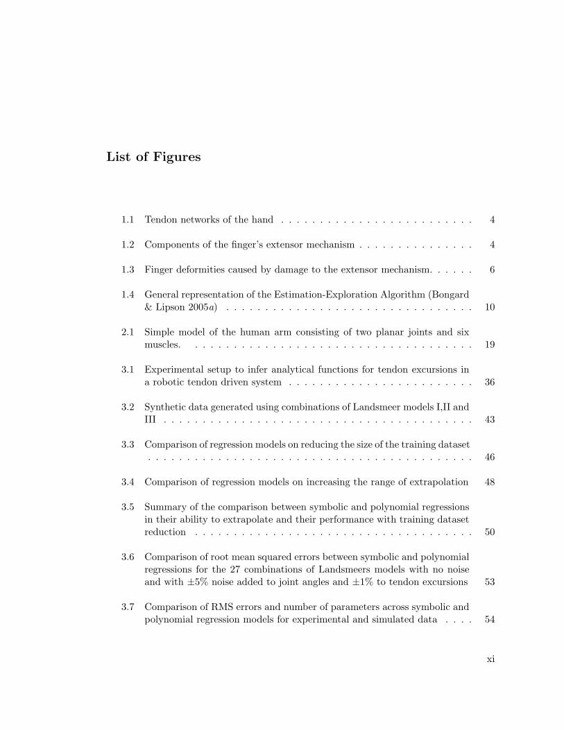
List of Figures

1.1 Tendon networks of the hand . . . . . . . . . . . . . . . . . . . . . . . . . 4

1.2 Components of the finger’s extensor mechanism . . . . . . . . . . . . . . . 4

1.3 Finger deformities caused by damage to the extensor mechanism. . . . . . 6

1.4 General representation of the Estimation-Exploration Algorithm (Bongard& Lipson 2005a) . . . . . . . . . . . . . . . . . . . . . . . . . . . . . . . . 10

2.1 Simple model of the human arm consisting of two planar joints and sixmuscles. . . . . . . . . . . . . . . . . . . . . . . . . . . . . . . . . . . . . 19

3.1 Experimental setup to infer analytical functions for tendon excursions ina robotic tendon driven system . . . . . . . . . . . . . . . . . . . . . . . . 36

3.2 Synthetic data generated using combinations of Landsmeer models I,II andIII . . . . . . . . . . . . . . . . . . . . . . . . . . . . . . . . . . . . . . . . 43

3.3 Comparison of regression models on reducing the size of the training dataset. . . . . . . . . . . . . . . . . . . . . . . . . . . . . . . . . . . . . . . . . . 46

3.4 Comparison of regression models on increasing the range of extrapolation 48

3.5 Summary of the comparison between symbolic and polynomial regressionsin their ability to extrapolate and their performance with training datasetreduction . . . . . . . . . . . . . . . . . . . . . . . . . . . . . . . . . . . . 50

3.6 Comparison of root mean squared errors between symbolic and polynomialregressions for the 27 combinations of Landsmeers models with no noiseand with ±5% noise added to joint angles and ±1% to tendon excursions 53

3.7 Comparison of RMS errors and number of parameters across symbolic andpolynomial regression models for experimental and simulated data . . . . 54

xi

4.1 Cadaveric actuation setup used for the inference of analytical models mod-eling tendon routing of the seven tendons of the index finger . . . . . . . . 66

4.2 Comparison of symbolic, polynomial and Landsmeer functions when testedon datasets from two different movement trials from the same cadavericspecimen to compare generalizability of functions across experimental trials. 72

4.3 Comparison of symbolic, polynomial and Landsmeer models when testedon datasets from two different cadaveric specimens to compare generaliz-ability of models across hands. . . . . . . . . . . . . . . . . . . . . . . . . 73

5.1 Experimental setup to control the index finger of a freshly frozen cadaverichand to produce flexion-extension motion . . . . . . . . . . . . . . . . . . 82

5.2 The experimental setup used to record fingertip forces from a freshly frozencadaveric hand . . . . . . . . . . . . . . . . . . . . . . . . . . . . . . . . . 84

5.3 Tendon excursions and tendon tensions for a single tap. . . . . . . . . . . 88

5.4 Finger equilibrium study: Proximity of tendon tensions to null space ofthe moment arm matrix . . . . . . . . . . . . . . . . . . . . . . . . . . . . 89

5.5 Fingertip trajectories for a simple tapping motion in unaffected and im-paired cases. . . . . . . . . . . . . . . . . . . . . . . . . . . . . . . . . . . . 99

6.1 The experimental setup used to record fingertip forces from a freshly frozencadaveric hand . . . . . . . . . . . . . . . . . . . . . . . . . . . . . . . . . 102

6.2 Results of experimental evaluation of existing biomechanical index fingermodels . . . . . . . . . . . . . . . . . . . . . . . . . . . . . . . . . . . . . . 104

6.3 Absolute magnitude and direction errors for the An-Chao Normative modelwhen tested with experimental data from a cadaveric index finger . . . . . 106

7.1 Validation of the tendon network simulator. . . . . . . . . . . . . . . . . . 112

7.2 Sensitivity analysis of fingertip force output to properties of the extensormechanism . . . . . . . . . . . . . . . . . . . . . . . . . . . . . . . . . . . 117

7.3 Comparison of experimental and simulated data for latex network drapedon hemisphere. . . . . . . . . . . . . . . . . . . . . . . . . . . . . . . . . . 119

7.4 Sensitivity analysis results showing deviation of fingertip force magnitudeand direction on perturbations of topology and parameter values . . . . . 120

xii

7.5 Flowchart of the algorithm used for the tendon network simulator . . . . 124

8.1 The experimental setup to record input tendon tensions and output fin-gertip forces . . . . . . . . . . . . . . . . . . . . . . . . . . . . . . . . . . . 131

8.2 The tendon network simulator and the properties of the extensor mecha-nism that were inferred . . . . . . . . . . . . . . . . . . . . . . . . . . . . 133

8.3 The estimation exploration algorithm that infers in parallel the best modelsfitting the data available and best tests to distinguish between optimalmodels. . . . . . . . . . . . . . . . . . . . . . . . . . . . . . . . . . . . . . 134

8.4 Comparison of fingertip force magnitude and direction errors of the bestfive inferred models vs. An-Chao normative model . . . . . . . . . . . . . 140

8.5 The best five inferred models obtained using the estimation-explorationalgorithm. . . . . . . . . . . . . . . . . . . . . . . . . . . . . . . . . . . . . 141

8.6 Inference of network topology and parameter values in simulation, . . . . 146

9.1 Demonstration of the problem of unobservability. . . . . . . . . . . . . . . 151

9.2 Unobservability/Non-uniqueness issue when dealing with experimental data152

9.3 Errors in fingertip force vector arising from coordinate transformation fromforce sensor to finger. . . . . . . . . . . . . . . . . . . . . . . . . . . . . . . 154

9.4 Errors in fingertip force vector arising due to model being an inaccuraterepresentation of the experimental system . . . . . . . . . . . . . . . . . . 155

9.5 Sensitivity of fingertip force vector to changes in angle between MCPflexion-extension and ad-abduction axes. . . . . . . . . . . . . . . . . . . . 156

xiii

Abstract

This dissertation presents novel computational methods to infer accurate functional mod-

els of musculoskeletal systems from minimal experimental data focussing on the tendon

networks of the human fingers as an example. State of the art biomechanical modeling

consists of assuming a fixed structure for the system being modeled and measurement or

regression of specific parameter values. However, the assumed structure may not be the

best representation of the system and hence lead to a functionally less-accurate model.

The objective here is to simultaneously infer both the structure and the parameter val-

ues directly from experimental input-output data. We present novel methods to infer

computational models of two kinds– analytical models capturing input-output behavior

without specifically modeling the mechanics of the system, and anatomy-based models

that explicitly capture the mechanics of interactions of the constitutive elements. Using

experimental data from a tendon-driven robotic system and synthetic data from simu-

lated musculoskeletal systems, a novel method based on symbolic regression using genetic

programming that simultaneously infers the form and parameter values of mathemati-

cal expressions is presented and shown to outperform polynomial regression, the state

of the art method used in musculoskeletal modeling. This method is then implemented

xiv

on experimental data collected from a cadaveric index finger to obtain accurate analyti-

cal functions for the tendon excursions of the seven tendons of the finger. Whether the

goal is to obtain accurate subject-specific models or to obtain generalizable models, the

functions obtained using this novel technique are more accurate than both polynomial

regressions and Landsmeer-based models, both of which have been used in the literature.

Experimental control of a cadaveric index finger to produce simple finger movements

gives some insight on how a muscle-like spring based control can be more advantageous

than using simple force or position control. Two different kinds of equilibria is demon-

strated in the human cadaveric index finger, for the first time to our knowledge, and their

relationship to the null space of the moment arm matrix is studied. An experimental

validation, of some common models of the index finger in their ability to predict fingertip

output is presented and it is shown that the fingertip force is sensitive to moment arm

values. A novel non-linear finite element method based solver is developed that can be

used to model the interactions of elastic tendon networks on arbitrarily shaped bones.

This solver which is validated using experimental data is then used to model the extensor

mechanism draped on the finger bones and a local sensitivity analysis is performed to see

how the fingertip force output is affected by changes to the properties of the network.

It is concluded that fingertip force output is most sensitive to topology and the resting

lengths of the bands of the extensor mechanism. Finally, a novel inference algorithm

that is based on the co-evolution of models and tests is used to infer the parameters and

topology of a 3 dimensional model of the extensor mechanism directly from cadaveric

data with minimal number of experimental data points through intelligent testing. It is

xv

shown that the inferred models are more accurate in predicting fingertip force magnitude

and direction compared to a model popularly used in the literature.

xvi

Chapter 1

Introduction

1.1 Background

Computational models are useful tools to understand the behavior of musculoskeletal

systems and have been extensively used by the biomechanics community for some time

now. They help us understand how movement and force are produced by the human

body, to test theories of motor control and to determine the states of a system that

cannot be measured experimentally. They are useful to simulate changes on injury or

disease and to predict outcomes of surgeries. Chapter 2 discusses the details on the uses

of musculoskeletal models and how they can be built. Most often, these models are built

based on anatomical observations, assumptions about the structure of the system and

measurement of some individual parameters through experimental studies. Many times

anatomical observations may be inaccurate or do not capture the mechanical/functional

behavior of the system. Also experimentally measuring all properties of the system is not

always feasible. Hence there can be large discrepancies between the data and the model.

Most cases these models are not validated with experimental data. This dissertation

1

focuses on the concept of inference of musculoskeletal models directly from experimental

data with few assumptions about the structure and parameter values. The hypothesis is

that models inferred from experimental input-output data would more accurately capture

the functional behavior of the system than these existing models based on assumptions

about the anatomy. Inference of such models requires a combination of tools from care-

fully measured experimental data consisting of system inputs and outputs to a modeling

environment where these musculoskeletal systems can be represented, to inference al-

gorithms that can estimate the structure and parameters of these models directly from

experimental data. With advances in the field of electromechanical actuation, computa-

tional mechanics, machine learning, artificial intelligence and optimization, we are at a

unique position to combine these different tools to develop informative models of these

complex systems. This dissertation demonstrates new inference methods to learn mod-

els of musculoskeletal systems from experimental data using the tendon networks of the

fingers as an example.

1.2 Modeling the Human Tendon Networks

Finger joint motion and fingertip force production are critical to the activities of daily liv-

ing. These are produced by the coordinated actuation of multiple finger muscles through

the intricate network of interconnections constituting the extensor mechanism. How these

different finger muscles coordinate to produce finger motion and force is still an unan-

swered question. While it is important to understand the neural control of the muscles

actuating the fingers, it is also critical to understand the role of passive biomechanical

2

tissue that transfers forces from the muscles to the finger joints. In fact, developing and

testing theories of neural control heavily depend on a good representation of the ‘plant’.

1.2.1 Anatomy

Tendons in most parts of the body connect a single muscle to a single point of attachment

on the bone. In the hand, tendons form complex networks of interconnections that

connect multiple muscles to multiple points of attachment on the bones. These networks

exist within a single finger (i.e. the extensor mechanism, Fig. 1.1(a)) as well as across

multiple fingers (i.e. the junctura tendinae, Fig. 1.1(b)). The finger musculature is able

to coordinate finger movement and finger force production by transmitting forces through

this intricate network of collagenous fibers.

Fig. 1.2 shows the main components of the extensor mechanism of the fingers. It

consists of bands of collagenous fibers that transfer forces from three main sets of inputs

to two tendon slips, the central and terminal slip, that actuate the joints. In the case

of the index finger, these three inputs come from four muscles : the extensor indicis,

extensor digitorum communis, first palmar interosseous and the lumbrical.

1.2.2 Functional Significance of the Extensor Mechanism

Clinicians, anatomists, biomechanists and neurophysiologists have been interested in un-

derstanding the role of the tendon networks in human manipulation for several decades

now (Haines 1951, Landsmeer 1949, Schieber & Santello 2004, Valero-Cuevas 2005, Brand

& Hollister 1999). Most studies so far have been qualitative analyses of the func-

tional significance of the extensor mechanism based on testing of cadaveric specimens

3

Netter, F. Atlas of Human Anatomy, 3rd edition, pp 447-453

(a) Extensor mechanism of the finger

Grant, J. C. B. and J.E. Anderson (1978). “Grant’s atlas of anatomy”, Williams & Wilkins

(b) Juncturae tendinae across fingers

Figure 1.1: Tendon networks of the hand

Lateral bands

Central slip

Terminal slip

Retinacular ligament

Sagittal band

Transverse fibers

Clavero et al. (2003). “Extensor Mechanism of the Fingers: MR Imaging-Anatomic Correlation”, Radiographics

Figure 1.2: (Clavero et al. 2003)

4

(Smith 1974, Landsmeer 1949, Harris Jr & Rutledge Jr 1972, Littler 1967). These studies

have shown that the extensor mechanism produces anatomical coupling of interphalangeal

joint rotations (Landsmeer 1963, Harris Jr & Rutledge Jr 1972) and its absence causes

the interphalangeal joints to flex sequentially and not in unison (Brand & Hollister 1999).

There have been simplistic 2D planar models of the extensor mechanism that have also

tried to demonstrate this effect (Spoor & Landsmeer 1976, Leijnse, Bonte, Landsmeer,

Kalker, Van der Meulen & Snijders 1992, Leijnse 1996, Kamper, George Hornby &

Rymer 2002). The contribution of the extensor mechanism versus neural factors to-

wards interphalangeal coupling is still not clear (Darling, Cole & Miller 1994, Kuo, Lee,

Jindrich & Dennerlein 2006).

Several studies have focussed on understanding the geometric and tensile proper-

ties of the different components of the extensor mechanism(Landsmeer 1949, Haines

1951, Garcia-Elias, An, Berglund, Linscheid, Cooney Iii & Chao 1991, Garcia-Elias, An,

Berglund, Linscheid, Cooney & Chao 1991). It has been shown that the relative ori-

entation of the different bands of the extensor mechanism vary significantly with finger

posture, thus changing the effective moment arm of the extensor mechanism about the

interphalangeal joints (Garcia-Elias, An, Berglund, Linscheid, Cooney Iii & Chao 1991).

The force distribution through the different bands of the extensor mechanism also changes

significantly with finger posture; the lateral bands transmitting majority of the force in

the extended posture and the central and terminal bands transferring majority of the force

in the flexed posture (Sarrafian, Kazarian, Topouzian, Sarrafian & Siegelman 1970, Micks

& Reswick 1981).

5

The clinical significance of understanding the function of the extensor mechanism

cannot be overstated (Bunnell 1945, Brand & Hollister 1999, Zancolli 1979). Even slight

damage to these networks leads to finger deformities and loss of function (Stark, Boyes

& Wilson 1962, Littler 1967, Rockwell, Butler & Byrne 2000). Two of the most common

finger deformities caused due to damage of the extensor mechanism are the boutonniere

deformity (Fig. 1.3(a)) and the mallet finger (Fig. 1.3(b)).The boutonniere deformity

occurs due to rupture of the central slip of the extensor mechanism and the mallet finger

deformity due to rupture of the terminal slip. Also other finger deformities like the swan

neck deformity caused due to inflammation of the proximal interphalangeal (PIP) joint

during rheumatoid arthritis results in force imbalance in the extensor mechanism leading

to loss of function. How the different components of the extensor mechanism contribute to

force transmission and how forces redistribute upon damage has still not been understood.

http://www.davidlnelson.md

(a) Boutonniere deformity

http://www.handspecialists.com/

(b) Mallet finger

Figure 1.3: Finger deformities caused by damage to the extensor mechanism.

6

1.3 Previous Work

The Winslow’s rhombus representation originally described by Winslow and reproduced

in drawing by Zancolli (Zancolli 1979) has been the generally accepted representation

for the extensor mechanism, though there have been alternative descriptions that have

been suggested in the literature(Garcia-Elias, An, Berglund, Linscheid, Cooney Iii &

Chao 1991, Garcia-Elias, An, Berglund, Linscheid, Cooney & Chao 1991). This model

(the Winslow’s rhombus) was based on qualitative anatomical observations in cadaveric

tissue and no quantitative proof exists even today if this is a good functional represen-

tation of the real structure. Hence there is need to either validate this model in its

ability to reproduce experimental data or suggest alternative, more accurate, functional

models. The reason why Winslow’s model representation has not been validated so far

is largely because of the computational complexity involved in modeling a deformable

elastic network wrapped on a set of irregular bones and also because obtaining extensive

experimental data from cadaveric specimens is very difficult.

The work of An and Chao on modeling hand function was one of the early compu-

tational studies to employ the Winslow’s rhombus representation to model the exten-

sor mechanism (An, Chao, Cooney & Linscheid 1979, An, Chao, Cooney & Linscheid

1985, Chao & An 1978a). These studies assumed a fixed distribution of tendon ten-

sions among the different bands of the extensor mechanism for all postures. This model

was later used in other studies as well (Li, Zatsiorsky & Latash 2001, Harding, Brandt &

Hillberry 1993, Dennerlein, Diao, Mote Jr & Rempel 1998, Weightman & Amis 1982). But

earlier studies had shown that the geometry of the bands as well as the force distribution

7

through them, change significantly with posture (Garcia-Elias, An, Berglund, Linscheid,

Cooney Iii & Chao 1991, Sarrafian et al. 1970, Micks & Reswick 1981). Hence a 3D

‘floating net’ model was suggested by Valero-Cuevas et al. where the tension distribution

in the different bands would vary with posture (Valero-Cuevas, Zajac & Burgar 1998).

They found that only when they allowed the distribution of tensions to change with

posture that the finger model could accurately predict the measured maximal isometric

forces and the coordination patterns that produced them. Two dimensional planar mod-

els of the finger have also used a simplified Winslow’s rhombus representation (Leijnse

et al. 1992, Leijnse 1996, Spoor 1983). But two dimensional models combine the lum-

brical and interossei tendons as one tendon, do not include ad-abduction of the finger

and they cannot capture all the interdependencies of the different bands of the extensor

mechanism.

Recently, Sueda et al. have developed a dynamic simulator of hand motion that models

the tendon networks in three dimensions (Sueda, Kaufman & Pai 2008). Tendinous

connections are represented as cubic splines and their interactions with bones are modeled

by line and surface constraints. This model, developed mainly for the graphics community,

aims to produce physically realistic simulations of hand motion and has not been validated

for its functional accuracy in modeling finger motion and force data. The predecessor

to the computational simulator that we have developed here, is the one developed by

Valero-Cuevas and Lipson that is based on the relaxation algorithm (Valero-Cuevas &

Lipson 2004, Valero-Cuevas, Anand, Saxena & Lipson 2007, Valero-Cuevas, Yi, Brown,

McNamara, Paul & Lipson 2007, Lipson 2006). This simulator uses simple cylinders to

models bones and is computationally slow.

8

Other finger dynamic models use analytical functional representations for the different

components of the tendon networks (Brook, Mizrahi, Shoham & Dayan 1995, Buchner,

Hines & Hemami 1988, Sancho-Bru, Perez-Gonzalez, Vergara-Monedero & Giurintano

2001). These analytical expressions, derived by Landsmeer based on geometry, map joint

angles to tendon excursions (Landsmeer 1961). While these functional models may be con-

venient for dynamic modeling and for purposes of control, they do not capture the physics

of interaction of the different components of the extensor mechanism. Also these models

have not been validated with experimental data. Most full body musculoskeletal model-

ing software like SIMM (Motion Analysis Corporation) (Delp & Loan 1995), AnyBody

(AnyBody Technology) (Damsgaard, Rasmussen, Christensen, Surma & de Zee 2006) and

MSMS (Davoodi, Urata, Hauschild, Khachani & Loeb 2007) do not model the tendon

networks of the hand. We have described the steps involved in computational modeling

of biomechanical systems and provided an overview of current methods in our recently

published review article (Valero-Cuevas, Hoffmann, Kurse, Kutch & Theodorou 2009).

The estimation-exploration algorithm is an active machine learning technique based on

coevolution that has been used successfully for the inference of the topologies and parame-

ter values of several complex nonlinear systems through minimum experimentation(Bongard

& Lipson 2005a, Bongard & Lipson 2005b, Bongard & Lipson 2004a, Bongard & Lipson

2004b, Lipson, Bongard, Zykov & Malone 2006).

The same algorithm has also been successfully employed for the inference of the struc-

ture of the extensor mechanism in two dimensions with simulated data generated by

a hidden target network as well as data from synthetic networks and cadaveric tissue

9

Figure 1.4: General representation of the Estimation-Exploration Algorithm (Bongard& Lipson 2005a)

(Valero-Cuevas, Anand, Saxena & Lipson 2007). This is briefly described in section

1.3.1.

1.3.1 Prior Work in the Lab Leading to Current Work

• Importance in motor control : It was shown using cadaveric experimental data and

in computer simulations that the extensor mechanism could be performing a com-

plex transformation from muscle forces to finger joint torques. Hence, understand-

ing the function of these passive structures is critical for the development of theories

of motor control (Valero-Cuevas, Yi, Brown, McNamara, Paul & Lipson 2007).

• Importance of topology: Using a three-dimensional computational model of the

extensor mechanism draped on bones, it was shown that the output of the finger

critically depends on the assumed topology of the network(Valero-Cuevas, Anand,

Saxena & Lipson 2007, Valero-Cuevas, Yi, Brown, McNamara, Paul & Lipson 2007).

10

Hence computational models of the hand being developed to understand finger

function would require accurate representations of the extensor mechanism topology.

• Inference of network topologies from simulated data in 2D : The topologies of hid-

den, two dimensional, elastic networks were inferred from simulated data (Valero-

Cuevas, Anand, Saxena & Lipson 2007). It was shown that the estimation-exploration

algorithm required fewer experimental tests and converged to more accurate func-

tional representations of the hidden elastic networks in comparison to random test-

ing.

• Inference of planar two dimensional networks from experimental data : The topolo-

gies of planar, synthetic, elastic networks were inferred from experimental data

generated by sequential loading of these networks. This demonstrated that the

estimation-exploration algorithm could be successfully employed in the inference

of complex network topologies even with noisy experimental data (Manuscript in

review).

• Inference of the topology of the extensor mechanism in two dimensions : The topol-

ogy of the extensor mechanism in two dimensions was successfully inferred using the

estimation-exploration algorithm from experimental data collected by differential

loading of cadaveric tissue. This was further proof that the estimation-exploration

algorithm can be successfully used for the inference of topology and parameters of

complex biological systems (Manuscript in review)..

11

1.4 Significance of Research

This dissertation presents novel methods for the development of computational models of

musculoskeletal systems, specifically focussing on the tendinous networks of the human

fingers. It combines experimental studies of human cadaveric specimens with mathemat-

ical analyses, solid mechanics and novel inference algorithms to develop computational

models of two kinds : analytical functional models and anatomy-based models. The

methods of computational modeling presented here make contributions to the areas of

motor control, clinical research, evolutionary understanding of biomechanical systems and

in the development of robotics and prosthetics.

Understanding motor control of human movement and force require accurate math-

ematical representations of the ‘plant’. The inference of compact, analytical functions

modeling tendon routing in musculoskeletal systems and the specific models for the index

finger presented here enable the development of dynamical models to test theories of mo-

tor control. Cadaveric control of the index finger to produce simple finger movements as

well as the observation of two forms of equilibria in specific postures and tendon tension

combinations contributes to our understanding of finger movement control. While there

have been several simplified representations of the tendon networks of the fingers, none of

the existing representations actually model the physics of interactions of these networks

with the bones. The finite element solver presented here would allow clinicians and re-

searchers to mathematically understand how the different components of these networks

help transform forces generated by the muscles to end point fingertip force. Simulation of

injury and damage to these networks could help predict changes in force transformation

12

and help surgeons plan repair and surgery to restore function in the fingers. Simulat-

ing different network topologies, node positions and elastic properties of the extensor

mechanism throws light on the significance and uniqueness of the existing structure from

an evolutionary perspective. The estimation exploration algorithm implemented here to

optimize models of the extensor mechanism with minimal experimentation is a step to-

wards development of subject-specific musculoskeletal models through intelligent testing.

The ultimate goal would be to infer accurate subject-specific models of musculoskeletal

systems in human subjects by performing only those tests that provide most information

about the system being modeled.

1.5 Dissertation Outline

1.5.1 Chapter 2

This chapter reviews musculoskeletal modeling literature and demonstrates the steps in-

volved in constructing a musculoskeletal model using the example of the human arm. This

formed a part of the section on musculoskeletal modeling that I wrote in the review paper

(Valero-Cuevas et al. 2009) published in the IEEE Reviews in Biomedical Engineering.

Dr. Francisco J. Valero-Cuevas is a co-author of this section.

1.5.2 Chapter 3

This chapter presents a novel method based on symbolic regression using genetic program-

ming to simultaneously infer both the form and parameter values of analytical functions

describing tendon excursions and moment arms in musculoskeletal systems. Using (i)

13

experimental data from a physical tendon-driven robotic system with arbitrarily routed

multiarticular tendons and (ii) synthetic data from musculoskeletal models, it is shown

that these analytical functions outperforms polynomial regressions in the amount of train-

ing data, ability to extrapolate, robustness to noise, and representation containing fewer

parameters – all critical to realistic and efficient computational modeling of complex mus-

culoskeletal systems. This is a paper that was published in the IEEE Transactions on

Biomedical Engineering (Kurse, Lipson & Valero-Cuevas 2012). Dr. Hod Lipson and Dr.

Francisco J. Valero-Cuevas are co-authors.

1.5.3 Chapter 4

This chapter presents the application of the above method to infer analytical functions

for the tendon excursions in a human index finger from cadaveric experimental data. It

demonstrates that these inferred models are more accurate and have fewer parameters

compared to both polynomial regressions and models based on geometry, whether the

goal is to obtain subject-specific models or models that generalize across subjects. Dr.

Hod Lipson and Dr. Francisco J. Valero-Cuevas are co-authors.

1.5.4 Chapter 5

This chapter presents the use of the tendon actuation system to control a human index

finger to produce slow tapping motion. It also demonstrates a specific kind of equilibrium

(what we term neutral equilibrium) in specific finger postures and combinations of tendon

tensions which are shown to lie in the null space of the finger’s moment arm matrix in

those postures. Dr. Jason Kutch and Dr. Francisco J. Valero-Cuevas are co-authors.

14

1.5.5 Chapter 6

Three existing models of the human index finger are evaluated with experimental data.

It is shown that fingertip output is sensitive to moment arm values and these existing

models diverge from experimental data necessitating more accurate representations. This

was presented at the American Society of Biomechanics conference 2011 at Long Beach.

Dr. Hod Lipson and Dr. Francisco J. Valero-Cuevas are co-authors.

1.5.6 Chapter 7

A novel nonlinear finite element method based tendon network simulator is presented,

validated with experimental data and used to study the sensitivity of the fingertip force

output to the topology and parameters of the finger’s extensor mechanism. Dr. Hod

Lipson and Dr. Francisco J. Valero-Cuevas are co-authors.

1.5.7 Chapter 8

Three dimensional models of the finger’s extensor mechanism topology and parameter

values are inferred directly from experimental data collected from a cadaveric index finger

through intelligent testing using the estimation-exploration algorithm. Dr. Hod Lipson

and Dr. Francisco J. Valero-Cuevas are co-authors.

1.5.8 Chapter 9

Chapter 9 discusses some of the challenges faced in the inference of computational models

of the tendon networks from experimental data.

15

1.5.9 Chapter 10

Chapter 10 discusses conclusions and future work.

16

Chapter 2

Fundamentals of Biomechanical Modeling

Computational models of the musculoskeletal system (i.e., the physics of the world and

skeletal anatomy, and the physiological mechanisms that produce muscle force) are a

necessary foundation when building models of neuromuscular function. Musculoskeletal

models have been widely used to characterize human movement and understand how

muscles can be coordinated to produce function. While experimental data are the most

reliable source of information about a system, computer models can give access to pa-

rameters that cannot be measured experimentally and give insight on how these internal

variables change during the performance of the task. Such models can be used to sim-

ulate neuromuscular abnormalities, identify injury mechanisms and plan rehabilitation

(Neptune 2000, McLean, Su & van den Bogert 2003, Fregly 2008). They can be used by

surgeons to simulate tendon transfer (Herrmann & Delp 1999, Magermans, Chadwick,

Veeger, Rozing & Van der Helm 2004, Valero-Cuevas & Hentz 2002) and joint replace-

ment surgeries (Piazza & Delp 2001), to analyze the energetics of human movement

(Kuo 2002), athletic performance (Hull & Jorge 1985), design prosthetics and biomedical

implants (Huiskes & Chao 1983), and functional electric stimulation controllers (Schutte,

17

Rodgers, Zajac, Glaser, Center & Alto 1993, Davoodi, Brown & Loeb 2003, Davoodi &

Loeb 2003).

Naturally, the type, complexity and physiological accuracy of the models vary depend-

ing on the purpose of the study. Extremely simple models that are not physiologically

realistic can and do give insight into biological function (e.g., (Garcia, Chatterjee, Ruina

& Coleman 1998)). On the other hand, more complex models that describe the physiol-

ogy closely might be necessary to explain some other phenomenon of interest (Van der

Helm 1994). Most models used in understanding neuromuscular function lie in-between,

with a combination of physiological reality and modeling simplicity. While several pa-

pers (Pandy 2001, Zajac 2002, Zajac, Neptune & Kautz 2002, Buchanan, Lloyd, Manal

& Besier 2004, Hatze 2005, Thelen, Anderson & Delp 2003, Piazza 2006, Fernandez &

Pandy 2006) and books (Winter 1990, Winters 2000, Yamaguchi 2005) discuss the im-

portance of musculoskeletal models and how to build them, we will give a brief overview

of the necessary steps and discuss some commonly performed analyses and limitations

using these models. We will illustrate the procedure for building a musculoskeletal model

by considering the example of the human arm consisting of the forearm and upper arm

linked at the elbow joint as shown in Fig. 2.1.

2.1 Computational Environments

The motivation and advantage of graphical/computational packages like SIMM (Motion

Analysis Corporation), AnyBody (AnyBody Technology), MSMS, etc. (Delp & Loan

1995, Davoodi et al. 2003, Damsgaard et al. 2006) is to build graphical representations

18

6

5 4

2

1

3

Figure 2.1: Simple model of the human arm consisting of two planar joints and sixmuscles.

of musculoskeletal systems, and translate them into code that is readable by multibody

dynamics computational packages like SDFast (PTC), Autolev (Online Dynamics Inc.),

ADAMS (MSC Software Corp.), MATLAB (Mathworks Inc.), etc. or use their own

dynamics solvers. These packages allow users to define musculoskeletal models, calculate

moment arms and musculotendon lengths, etc.

This engineering approach dates back to the use of computer aided design tools and

finite element analysis packages to study bone structure and function in the 60’s, which

grew to include rigid body dynamics simulators in the mid 80’s like ADAMS and Au-

tolev. Before the advent of these programming environments (as in the case of computer

aided design), engineers had to generate their own equations of motion or Newtonian

analysis by hand, and write their own code to solve the system for the purpose of inter-

est. Available packages for musculoskeletal modeling have now empowered researchers

without training in engineering mechanics to assemble and simulate complex nonlinear

dynamical systems. The risk, however, is that the lack of engineering intuition about how

19

complex dynamical systems behave can lead the user to accept results that one otherwise

would not. In addition, to our knowledge, multibody dynamics computational packages

have not been cross-validated against each other, or a common standard, to the extent

that finite elements analysis code has (Anderson, Ellis & Weiss 2007) and the simulation

of nonlinear dynamical systems remains an area of study with improved integrators and

collision algorithms developed every year. An exercise the user can do is to simulate the

same planar double or triple pendulum (i.e., a limb) in different multi-body dynamics

computational packages and compare results after a few seconds of simulation. The dif-

ferences are attributable to the nuances of the computational algorithms used, which are

often beyond the view and control of the user. Whether these shortcomings in dynamical

simulators affect the results of the investigation can only be answered by the user and

reviewers on a case-by case basis, and experts can also disagree on computational results

in the mainstream of research like gait analysis (Neptune, Kautz & Zajac 2001, Neptune,

Zajac & Kautz 2004, Kuo & Maxwell Donelan 2009).

2.2 Dimensionality and Redundancy

The first decision to be made when assembling a musculoskeletal model is to define dimen-

sionality of the musculoskeletal model (i.e., number of kinematic degrees-of-freedom and

the number of muscles acting on them). If the number of muscles exceeds the minimal

number required to control a set of kinematic degrees-of-freedom, the musculoskeletal

model will be redundant for some sub-maximal tasks. The validity and utility of the

model to the research question will be affected by the approach taken to address muscle

20

redundancy. Most musculoskeletal models have a lower dimensionality than the actual

system they are simulating because it simplifies the mathematical implementation and

analysis, or because a low-dimensional model is thought sufficient to simulate the task be-

ing analyzed. Kinematic dimensionality is often reduced to limit motion to a plane when

simulating arm motion at the level of the shoulder (Abend, Bizzi & Morasso 1982, Mussa-

Ivaldi, Hogan & Bizzi 1985, Shadmehr & Mussa-Ivaldi 1994), when simulating fingers

flexing and extending (Dennerlein, Diao, Mote Jr & Rempel 1998) or when simulating

leg movements during gait (Olney, Griffin, Monga & McBride 1991). Similarly, the num-

ber of independently controlled muscles is often reduced (An et al. 1985) for simplicity,

or even made equal to the number of kinematic degrees-of-freedom to avoid muscle re-

dundancy (Harding et al. 1993). While reducing the dimensionality of a model can be

valid in many occasions, one needs to be careful to ensure it is capable of replicating

the function being studied. For example, an inappropriate kinematic model can lead to

erroneous predictions (Valero-Cuevas, Towles & Hentz 2000, Jinha, Ait-Haddou, Binding

& Herzog 2006), or reducing a set of muscles too severely may not be sufficiently realistic

for clinical purposes.

A subtle but equally important risk is that of assembling a kinematic model with a

given number of degrees of freedom, but then not considering the full kinematic output.

For example, a three-joint planar linkage system to simulate a leg or a finger has three

kinematic degrees of freedom at the input, and also three kinematic degrees of freedom

at the output: the x and y location of the endpoint plus the orientation of the third link.

As a rule, the number of rotational degrees-of-freedom (i.e., joint angles) maps into as

many kinematic degrees-of-freedom at the endpoint (Murray, Li & Sastry 1994). Thus,

21

for example, studying muscle coordination to study endpoint location without considering

the orientation of the terminal link can lead to variable results. As we have described in

the literature (Valero-Cuevas et al. 1998, Valero-Cuevas 2009), the geometric model and

Jacobian of the linkage system need to account for all input and output kinematic degrees-

of-freedom to properly represent the mapping from muscle actions to limb kinematics and

kinetics.

2.3 Skeletal Mechanics

In neuromuscular function studies, skeletal segments are generally modeled as rigid links

connected to one another by mechanical pin joints with orthogonal axes of rotation. These

assumptions are tenable in most cases, but their validity may depend on the purpose of the

model. Some joints like the thumb carpometacarpal joint, the ankle and shoulder joints

are complex and their rotational axes are not necessarily perpendicular (Hollister, Bu-

ford, Myers, Giurintano & Novick 1992, Inman 1944, Van Langelaan 1983), or necessarily

consistent across subjects (Hollister et al. 1992, Santos & Valero-Cuevas 2006, Cerveri,

De Momi, Marchente, Lopomo, Baud-Bovy, Barros & Ferrigno 2008). Assuming sim-

plified models may fail to capture the real kinematics of these systems (Valero-Cuevas,

Johanson & Towles 2003). While passive moments due to ligaments and other soft tissues

of the joint are often neglected, at times they are modeled as exponential functions of

joint angles (Yoon & Mansour 1982, Hatze 1997) at the extremes of range of motion to

passively prevent hyper-rotation. In other cases, passive moments well within the range

of motion could be particularly important in the case of systems like the fingers (Esteki

22

& Mansour 1996, Sancho-Bru et al. 2001) where skin, fat and hydrostatic pressure tend

to resist flexion.

Modeling of contact mechanics could be important for joints like the knee and the

ankle where there is significant loading on the articulating surfaces of the bones, and where

muscle force predictions could be affected by contact pressure. Joint mechanics are also of

interest for the design of prostheses, where the knee or hip could be simulated as contact

surfaces rolling and sliding with respect to each other (Bartel, Bicknell & Wright 1986,

Rawlinson & Bartel 2002, Rawlinson, Furman, Li, Wright & Bartel 2006). Several studies

estimate contact pressures using quasi-static models with deformable contact theory (e.g.,

(Wismans, Veldpaus, Janssen, Huson & Struben 1980, Blankevoort, Kuiper, Huiskes &

Grootenboer 1991, Pandy, Sasaki & Kim 1997, Pandy & Sasaki 1998)). But these models

fail to predict muscle forces during dynamic loading. Multibody dynamic models with

rigid contact fail to predict contact pressures (Piazza & Delp 2001).

For the illustrative example carried throughout this review we will use the simple

two-joint, six-muscle planar limb shown in Fig. 2.1. We model the upper arm and the

forearm as two rigid cylindrical links connected to each other by a pin joint representing

the elbow and shoulder joints as hinges. We will neglect moment due to passive structures

and assume frictionless joints. We will not consider any contact mechanics at the joints.

This model will simulate the movement and force production of the hand (i.e., a fist with a

frozen wrist) in a two-dimensional plane perpendicular to the torso as is commonly done in

studies of upper extremity function (Abend et al. 1982, Mussa-Ivaldi et al. 1985, Shadmehr

& Mussa-Ivaldi 1994).

23

2.4 Musculotendon Routing

Next, we need to select the routing of the musculotendon unit consisting of a muscle and

its tendon in series (Zajac, Biosci, Physiol, Biol, Physiol, Lond, Physiol, Soc, Acta &

Biochem 1989, Zajac 1992). The reason we speak in general about musculotendons (and

not simply tendons) is that in many cases it is the belly of the muscle that wraps around

the joint (e.g., gluteus maximus over the hip, medial deltoid over the shoulder). In other

cases, however, it is only the tendon that crosses any joints as in the case of the patellar

tendon of the knee or the flexors of the wrist. In addition, the properties of long tendons

affect the overall behavior of muscle like by stretching out the force-length curve of the

muscle fibers (Zajac et al. 1989). Most studies assume correctly that musculotendons

insert into bones at single points or multiple discrete points (if the actual muscle attaches

over a long or broad area of bone). Musculotendon routing defines the direction of travel

of the force exerted by a muscle when it contracts. This defines the moment arm r of a

muscle about a particular joint, and determines both the excursion δs the musculotendon

will undergo as the joint rotates an angle δθ defined by the equation, δs = r ∗ δθ, as well

as the joint torque τ at that joint due to the muscle force fm transmitted by the tendon

τ = r ∗ fm where r is the minimal perpendicular distance of the musculotendon from the

joint center for the planar (scalar) case (Zajac 1992). For the three dimensional case the

torque is calculated by the cross product of the moment arm with the vector of muscle

force τ = r× fm.

In today’s models, musculotendon paths are modeled and visualized either by straight

lines joining the points of attachment of the muscle; straight lines connecting “via points”

24

attached to specific points on the bone which are added or removed depending on joint

configuration (Garner & Pandy 2000) or as cubic splines with sliding and surface con-

straints (Sueda et al. 2008). Several advances also allow representing muscles as volumet-

ric entities with data extracted from imaging studies (Blemker & Delp 2005, Blemker,

Asakawa, Gold & Delp 2007), and defining tendon paths as wrapping in a piecewise linear

way around ellipses defining joint locations (Delp & Loan 1995, Davoodi et al. 2003). The

path of the musculotendon in these cases is defined based on knowledge of the anatomy.

Sometimes, it may not be necessary to model the musculotendon paths but obtaining

a mathematical expression for the moment arm (r) could suffice. The moment arm is

often a function of joint angle and can be obtained by recording incremental tendon

excursions (δs) and corresponding joint angle changes (δθ) in cadaveric specimens (Eg.

(Otis, Jiang, Wickiewicz, Peterson, Warren & Santner 1994, An, Ueba, Chao, Cooney &

Linscheid 1983)).

For the arm model example (Fig. 2.1), we will model musculotendon paths as straight

lines connecting their points of insertion. We will attach single-joint flexors and extensors

at the shoulder (pectoralis and deltoid) and elbow (biceps long head and triceps lateral

head) and double-joint muscles across both joints (biceps short head and triceps long

head). Muscle origins and points of insertion are estimated from the anatomy. In our

model of the arm in Fig. 2.1, we shall model musculotendons as simple linear springs.

We then assign values to model parameters like segment inertia, elastic properties of

the musculotendons, etc. At this point the model is complete and ready for dynamical

analysis.

25

2.5 Musculotendon Models

The most commonly used computational model of musculotendon force is the one based

on the Hill-type model of muscle(Zajac et al. 1989), largely because of its computational

efficiency, scalability, and because it is included in simulation packages like SIMM (Mo-

tion Analysis Corporation). In Hill-type models, the entire muscle is considered to behave

like a large sarcomere with its length and strength scaled-up, respectively, to the fiber

length and physiological cross sectional area of the muscle of interest. This model con-

sists of a parallel elastic element representing passive muscle stiffness, a parallel dashpot

representing muscle viscosity and a parallel contractile element representing activation-

contraction dynamics; all in series with a series elastic element representing the tendon.

The force generated by a muscle depends on muscle activation, physiological cross sec-

tional area of the muscle, pennation angle and force-length and force-velocity curves for

that muscle. These parameter values are generally based on animal or cadaveric work

(Lieber, Jacobson, Fazeli, Abrams & Botte 1992). Five parameters define the properties

of this musculotendon model. Four of these are specific to the muscle: the optimal mus-

cle fiber length, the peak isometric force (found by multiplying maximal muscle stress

by physiological cross-sectional area), the maximal muscle shortening velocity, and the

pennation angle. The fifth is the slack length of the tendon (tendon cross sectional area

is assumed to scale with its muscle’s physiological cross sectional area (An, Linscheid &

Brand 1991)). Model activation-contraction dynamics is adjusted to match the proper-

ties of slow or fast muscle fiber types by changing the activation and deactivation time

constants of a first order differential equation (Zajac et al. 1989). This Hill-type model

26

has undergone several modifications but remains a first-order approximation to muscle

as a large sarcomere with limited ability to simulate the full spectrum of muscles, or of

fiber types found within a same muscle, or the properties of muscle that arise from it be-

ing composed of populations of motor units such as signal dependent noise, etc. Several

researchers have developed alternative models for muscle contraction, which were used in

specific studies (Zahalak & Ma 1990, Karniel & Inbar 1997, Gonzalez, Hutchins, Barr &

Abraham 1996, Soechting & Flanders 1997).

The alternative approach has been to model muscles as populations of motor units.

While this is much more computationally expensive, it is done with the purpose of be-

ing more physiologically realistic and enabling explorations of other features of muscle

function. A well known model is that proposed by Fuglevand and colleagues (Fuglevand,

Winter & Patla 1993), which has been used extensively to investigate muscle physiol-

ogy, electromyography and force variability. However, the computational overhead of

this model has largely limited it to studies of single muscles, and is not usually part of

neuromuscular models of limbs. In order to develop a population-based model that could

be used easily by researchers, Loeb and colleagues developed the Virtual Muscle soft-

ware package (Cheng, Brown & Loeb 2000). It integrates motor recruitment models from

the literature and extensive experimentation with musculotendon contractile properties

into a software package that can be easily included in multibody dynamic models run in

MATLAB (The Mathworks, Natick, MA).

27

2.6 Forward and Inverse Simulations

In “forward” models, the behavior of the neuromuscular system is calculated in the nat-

ural order of events: from neural or muscle command to limb forces and movements. In

“inverse” models, the behavior is assumed or measured and the model is used to infer and

predict the time histories of neural, muscle or torque commands that produced it. The

same biomechanical model governed by Newtonian mechanics is used in either approach,

but it is used differently in each analysis (Yamaguchi 2005, Winter 1990).

2.6.1 Forward Models

The inputs to a forward musculoskeletal model are usually in the form of muscle activa-

tions (or torque commands if the model is torque driven) and the outputs are the forces

and/or movements generated by the musculoskeletal system. The system dynamics is

represented using the following equation,

M(q)q + C(q, q) +G(q) = R(q)FM + Fext(q, q) (2.1)

where M is the system mass matrix, q the vector of joint accelerations, q the vector

of joint angles, C the vector of Coriolis and centrifugal forces, G the gravitational torque,

R the instantaneous moment arm matrix, FM the vector of muscle forces and Fext, the

vector of external torques due to ground reaction forces and other environmental forces.

This system of ordinary differential equations is numerically integrated to obtain the

time course of all the states (joint angles q and joint angle velocities q) of the system.

28

The input muscle activations could be derived from measurements of muscle activity

(electromyogram) or from an optimization algorithm that minimizes some cost function,

for example the error in joint angle trajectory for all joints and energy consumed (Hatze

1977). Forward dynamics has also been used in determining internal forces that cannot

be experimentally measured like in the ligaments during activity or contact loads in

the joints. It gives insight on energy utilization, stability and muscle activity during

function for example in walking simulations (Neptune, McGowan & Kautz 2009). It

gives the user access to all the parameters of the system and to simulate effects when

these are changed. This makes it a useful tool to study pathological motion and for

rehabilitation. (Piazza 2006) provides a review on many of the applications of forward

dynamics modeling.

2.6.2 Inverse Models

Inverse dynamics consists of determining joint torque and muscle forces from experimen-

tally measured movements and external forces. Since the number of muscles crossing

a joint is higher than the degrees-of-freedom at the joint, multiple sets of muscle forces

could give rise to the same joint torques. This is the load-sharing problem in biomechanics

(Chao & An 1978b). A single combination is chosen by introducing constraints such that

the number of unknown variables is reduced and/or based on some optimization criterion,

like minimizing the sum of muscle forces or muscle activations. Several optimization crite-

ria have been used in the literature (Patriarco, Mann, Simon & Mansour 1981, Anderson

& Pandy 2001, Prilutsky & Zatsiorsky 2002). Muscle forces determined by this analysis

are often corroborated by electromyogram recordings from specific muscles (Kaufman,

29

An, Litchy & Chao 1991, Happee & Van der Helm 1995). Since inverse dynamics con-

sists of using the outputs of the real system as inputs to a mathematical model whose

dynamics don’t exactly match with the real system, the predicted behavior of the model

does not necessarily match with the measured behavior of the real system. This is an

important problem in inverse dynamics and is discussed in more detail in (Hatze 2002).

Both forward and inverse models are useful and can be complementary and the choice

is largely driven by the goals of the study. The main challenge with both these analyses is

experimental validation because many of the variables determined using either approach

cannot be measured directly. The reader is directed to articles and textbooks that describe

these methods in detail (Delp & Loan 1995, Delp, Anderson, Arnold, Loan, Habib, John,

Guendelman & Thelen 2007, Winter 1990, Davoodi et al. 2003, An, Chao & Kaufman

1991, Andriacchi, Natarajan & Hurwitz 1991).

30

Chapter 3

Extrapolatable Analytical Functions for Tendon Excursions

and Moment Arms from Sparse Datasets

3.1 Abstract

Computationally efficient modeling of complex neuromuscular systems for dynamics and

control simulations often requires accurate analytical expressions for moment arms over

the entire range of motion. Conventionally, polynomial expressions are regressed from

experimental data. But these polynomial regressions can fail to extrapolate, may require

large datasets to train, are not robust to noise, and often have numerous free parameters.

We present a novel method that simultaneously estimates both the form and parameter

values of arbitrary analytical expressions for tendon excursions and moment arms over

the entire range of motion from sparse datasets. This symbolic regression method based

on genetic programming has been shown to find the appropriate form of mathematical

expressions that capture the physics of mechanical systems. We demonstrate this method

by applying it to (i) experimental data from a physical tendon-driven robotic system with

arbitrarily routed multiarticular tendons and (ii) synthetic data from musculoskeletal

31

models. We show it outperforms polynomial regressions in the amount of training data,

ability to extrapolate, robustness to noise, and representation containing fewer parameters

– all critical to realistic and efficient computational modeling of complex musculoskeletal

systems.

3.2 Introduction

Computational modeling of complex musculoskeletal systems is sensitive to accurate rep-

resentation of tendon routing, insertion points, and moment arm values (Hoy, Zajac &

Gordon 1990, Valero-Cuevas et al. 2009). The most commonly used technique to obtain

moment arm variations over the range of motion of a joint is the tendon and joint displace-

ment method (An, Takahashi, Harrigan & Chao 1984). Implementation of this method

generally involves fitting explicit analytical expressions for tendon excursions as functions

of joint angles. Tendon excursions arise from changes in length of a musculotendon either

due to active contraction or passive stretching. Hence they are directly related to mus-

cle length changes and the maximal force a muscle can generate, as determined by the

force-length properties (Zajac et al. 1989). Moment arms over the range of motion can

then be obtained by taking partial derivatives of these tendon excursion expressions with

respect to the corresponding joint angle changes. This standard approach has been used

extensively in the literature to understand the contribution of different muscles towards

the production of joint torque and limb motion (Eg. (An et al. 1983, Spoor, Van Leeuwen,

Meskers, Titulaer & Huson 1990, Herzog & Read 1993, Liu, Hughes, Smutz, Niebur &

Nan-An 1997) ). It has also been used to validate musculoskeletal models representing

32

bone geometry and musculotendon pathways (Murray, Delp & Buchanan 1995, Buford Jr,

Ivey Jr, Malone, Patterson, Pearce, Nguyen & Stewart 1997). Simulation of musculoskele-

tal dynamics for the development and testing of theories of motor control also specifically

require analytical expressions for tendon excursions and moment arms as functions of

joint angles (Scott 2004, Valero-Cuevas et al. 2009). Very often, dynamic equations of

the system (which include the moment arm functions) need to be evaluated iteratively

(perhaps tens of thousands of times) to solve for an optimal control law for each cost

function and task goal (Theodorou, Todorov & Valero-Cuevas 2011). Such algorithms

require accurate, computationally-efficient analytical expressions for moment arms for the

entire range of motion.

Analytical expressions for moment arms and tendon excursions are of two kinds: (i)

Idealized geometric models, or (ii) Empirical models. The coefficients of the analytical

expressions in both these approaches are regressed from experimental data. These data

consist of joint angles and tendon excursion measurements, often obtained from cadav-

eric specimens (An et al. 1983, An et al. 1984, Spoor et al. 1990, Visser, Hoogkamer,

Bobbert & Huijing 1990, Pigeon, Yahia & Feldman 1996, Liu et al. 1997). In the first

case, idealized geometric models, tendon routings are approximated by simple geometric

shapes and the mathematical forms of the expressions are derived using trigonometry

(Eg. (Landsmeer 1961, Stern Jr 1971, Van Zuylen, Van Velzen & van der Gon 1988)).

While this might be sufficient to obtain approximate values of moment arms and tendon

excursions in some simple cases, it may not necessarily be accurate for all muscles and

is heavily dependent on assumptions about the anatomy. It is likely not appropriate for

33

the complex routing of many tendons around joints, as well as non-uniform bone geome-

try, deformity, surgical modification and injury. Therefore, most studies in biomechanics

use the second approach: empirical models. These almost always consist of polyno-

mial expressions (including splines, which are piecewise polynomials stitched together)

mapping joint angles to tendon excursions, and are regressed from experimental measure-

ments, such as using cadaveric specimens (Spoor et al. 1990, Visser et al. 1990, Pigeon

et al. 1996, Liu et al. 1997, Menegaldo, de Toledo Fleury & Weber 2004, Franko, Winters,

Tirrell, Hentzen & Lieber 2011). But these polynomial regressions have several inherent

mathematical pitfalls; they can fail to extrapolate, may require large datasets to train, are

not robust to noise, and often have numerous free parameters (Green & Silverman 1994).

Hence they may not be the best choice to model multi-degrees of freedom biomechanical

systems where (i) obtaining a rich dataset from the entire range of motion can be difficult

(Clewley, Guckenheimer & Valero-Cuevas 2008), (ii) data are generally sparse and con-

tain noise from measurement errors and skin deformations (Cappozzo, Catani, Leardini,

Benedetti & Della Croce 1996, Holden, Orsini, Siegel, Kepple, Gerber & Stanhope 1997),

and (iii) are susceptible to common errors in the estimation of axes of joint rotation

and accurate joint angles (Woltring, Huiskes & de Lange 1983). In addition, polynomial

functions are inherently a type of mathematical expression that is likely not reflective of

the geometry and physics of tendon routing which even in the ideal case often contain

trigonometric functions (Landsmeer 1961).

Here we present a novel method to find analytical functions for tendon excursions

and moment arms as functions of joint angles that does not assume a specific math-

ematical form apriori. Rather, it simultaneously estimates directly from experimental

34

data both appropriate mathematical forms of the analytical expressions for moment

arms and tendon excursions, and their best-fit parameter values. Previously we have

called attention to the need for biomechanical modeling to go beyond parameter esti-

mation and engage in the search for appropriate model forms (Valero-Cuevas, Anand,

Saxena & Lipson 2007). Here we show an example of how to perform this simultane-

ous search of mathematical form, i.e. the structure consisting of mathematical building

blocks; and parameter values, i.e. the coefficients and other constants accompanying

each building block of the mathematical expression, using a software package called Eu-

reqa (http://creativemachines.cornell.edu/eureqa). Eureqa implements symbolic regres-

sion using genetic programming (Schmidt & Lipson 2009). While symbolic regression and

genetic programming have been used for over 15 years (Koza 1992) in the field of machine

learning, Eureqa is a recent improvement that ensures faster convergence and more accu-

rate solutions (Schmidt & Lipson 2005, Schmidt & Lipson 2006). Unlike other machine

learning techniques that use a ‘black box’ approach to model input-output relationships,

Eureqa has been shown to obtain computationally efficient, analytical expressions that

can capture the physics of the system being modeled. In this chapter, we compare poly-

nomial regression (the state-of-the-art used by the musculoskeletal modeling community

to represent these systems) to our method. We apply the traditional polynomial regres-

sion approach and our novel machine learning method to both experimental data from

a multi-articular tendon-driven robotic system, and computer-generated synthetic data

from many simulated musculoskeletal systems with experimentally realistic noise added.

35

s1

s2

s3

2

1

3

Position encoders

Motors keeping tendons taut

Load cells

Motion capture markers

Motion capture camera

Figure 3.1: A three-joint planar robotic system with three arbitrarily routed tendonswas moved manually to span a range of joint angles. The tendon excursions wererecorded and joint angles calculated from motion capture data.

36

3.3 Methods

3.3.1 Symbolic Regression Using Genetic Programming

Symbolic regression is a machine learning technique that searches the space of mathe-

matical operators, functions and parameter values to obtain analytical expressions that

model available data based on a fitness criterion (Koza 1992). Evolutionary algorithms

are generally used to guide this search in what is an infinite dimensional space. Here

we use a software package called Eureqa that performs symbolic regression using genetic

programming to infer implicit and explicit analytical functions to model input-output

data (Schmidt & Lipson 2009). In our case, Eureqa searches for explicit analytical ex-

pressions of the form s = f(θ) mapping joint angles, θ to each tendon’s excursion s (Fig.

3.1). The three joint angles and the excursion of the tendon of interest at any time step

constitute a data point. Many such data points from the entire time series of the experi-

ment form a dataset. We use sum of deviations of inferred analytical function predictions

for the tendon excursions from true measurements (coming from experimental testing or

computer simulation) over an entire dataset as the fitness criterion, i.e. the fitness-error

to be minimized. In addition to this, Eureqa also penalizes the equation-complexity, de-

fined as the sum of the number of parameters and terms in the analytical expressions

being inferred. The search space consists of analytical expressions formed by parameter

values and combinations of mathematical operations performed on the input variables

(θ). In our case, we restricted the mathematical operations to addition, subtraction,

multiplication, division, sine, cosine, tangent and square root. Polynomial expressions

37

are automatically generated by repeated multiplication of the input variables. In addi-

tion, Eureqa uses the concept of coevolution of fitness predictors, described in detail in

(Schmidt & Lipson 2005), for faster and improved convergence of solutions. Instead of

using the entire time history of the training dataset to calculate the fitness of evolving

analytical expressions, it finds and uses a small set of data points (called fitness predic-

tors) that can best distinguish between analytical expressions of otherwise equal fitness.

Fitness predictors are chosen in every generation of evolution in parallel with the search

for analytical expressions modeling the experimental data.

Unlike conventional optimization that would minimize fitness-error in a ‘single line

search’ and find either the global minimum or one of the local minima of the fitness

landscape, Eureqa uses multi-objective optimization to produce a family of multiple ‘op-

timal’ analytical expressions (15-20 expressions) that map joint angles to the tendon

excursions. Each analytical expression has different levels of fitness-error and equation-

complexity (defined above). This family of analytical expressions constitutes a Pareto

front of fitness-error vs. equation-complexity. In this multi-objective optimization, the

tradeoffs between the fitness criteria are made explicit to the user. The advantage of

this approach is that it provides multiple analytical expressions that may be more or

less sparse, accurate, computationally efficient, or revealing of the physics of the problem

– either of which may be given more weight as ‘optimal’ by the user as desired. We

chose to define as the optimal solution the one analytical expression that had the low-

est extrapolation error (root mean squared error when tested with data points outside

the range of training datasets). However, the reader is free to weigh other aspects more

heavily. Our choice was driven by the need for analytical functions to have the ability

38

to extrapolate as it ensures that they are capturing the physics of the system; and not

simply overfitting to the training data points. Each search in Eureqa starts with an initial

set of multiple, random analytical functions, and terms are added/subtracted in discrete

steps as the search progresses. Eureqa provides the support to run a search very easily on

parallel computers that are connected in a network without requiring any special network

architecture or hardware. On average, we ran each search in parallel for 12 hours on 20

computers (Dual Dualcore AMD Opteron 2.0 GHz ) at the USC High-Performance Com-

puting and Communications (www.usc.edu/hpcc) computer cluster. As is necessary in

most machine learning problems without closed-form solutions, a stopping/convergence

criterion needs to be defined. We defined the search to have converged if the fitness of

the solution with the lowest fitness error remained unchanged for more than two hours.

We repeated the entire search five times to test for consistency of results. The family of

‘optimal’ solutions was not necessarily of identical form in every repeat but of different

representations of functions that modeled the data best with consistent RMS errors.

3.3.2 Comparison Against Polynomial Regression

The state-of-the-art technique is to regress tendon excursions as polynomial functions

of joint angles (Eg. (Spoor et al. 1990, Visser et al. 1990, Pigeon et al. 1996, Liu

et al. 1997, Menegaldo et al. 2004)). We regressed the coefficients of multivariable linear,

quadratic, cubic and quartic polynomials (all cross terms considered) using MATLAB

c© (Version R2009b, MathWorks, Natwick, MA). Polynomials of order greater than four

overfit to the training data and performed worse than polynomial regressions of lower

orders, and hence were not considered in this chapter. This is also the case with spline

39

functions, which are piecewise polynomials stitched together (Murray et al. 1995). More-

over, to evaluate dynamic equations of the system, for example to solve for an optimal

controller, simple analytical functions modeling the behavior of the system throughout

the range of motion are required. Splines or other piecewise surface fits would not be

not suitable for this purpose and hence were not considered in this chapter. We com-

pared the performance of analytical expressions from the multivariable linear, quadratic,

cubic and quartic regressions against those from symbolic regression by testing with a

cross-validation dataset (data points not selected for training, but within the range of

training) and an extrapolation dataset (data points outside the range of training). We

used root mean squared (RMS) error between the true tendon excursions (experimentally

measured or simulated) and the analytical function predictions (coming from symbolic

or polynomial regressions), normalized by the range of movement for that tendon and

expressed as a percentage, as the fitness error criterion for the comparison. RMS errors

were determined for cross-validation and extrapolation datasets.

3.3.3 Experimental Data from a Tendon-Driven Robotic System

We used a planar robotic finger with three links, three joints and three tendons to pro-

duce the motion capture data (Fig. 3.1). The three tendons were routed such that the

first tendon flexed all joints (similar in action to the flexor digitorum profundus in the

human finger), the second tendon, extended one joint and flexed the remaining two joints

(similar to an intrinsic tendon) and the third tendon, extended all joints (similar to the

extensor digitorum communis). We moved the robotic finger manually to span the full

three-dimensional joint configuration space of flexion-extension in a human finger. Servo

40

dc motors maintained a constant tension of 1.5 N in every tendon to prevent tendons

from going slack. As we moved the robotic finger, optical encoders measured tendon

excursions at a sampling frequency of 10Hz. A 6-camera optical motion capture system,

manufactured by Vicon (Lake Forest, CA), tracked reflective markers adhered to each

segment of the robotic finger at a frequency of 30 Hz. The mean calibration residual

error of the marker position reconstruction was less than 0.2 mm. We processed the 3D

coordinates of the markers generated by the Vicon Nexus software to obtain joint angle

changes for the entire duration of movement and then downsampled them to 10 Hz. We

then partitioned the datasets to test for robustness of the inferred analytical expressions

to (1) size of the training dataset and (2) range of extrapolation.

3.3.3.1 Reducing the Size of the Training Dataset

We divided the experimental data into training, cross-validation and extrapolation datasets

(training and cross-validation datasets coming from the same range of data and the ex-

trapolation dataset consisting of data points outside the range of training). Then, we

created nine independent training datasets by systematically reducing the number of

training data points keeping the range fixed (n, n/2, n/3, etc. in Fig. 3.3). We per-

formed symbolic and polynomial regressions using these nine different training datasets

and tested the resulting analytical expressions with the fixed cross-validation and extrap-

olation datasets. This was repeated five times for each training dataset, for each tendon

(S1, S2 and S3), by re-sampling the training data points with replacement (Eureqa picked

multiple random initial analytical functions at the beginning of each search). This was

done to ensure that the observed results were consistent and not simply due to chance.

41

3.3.3.2 Increasing the Range of Extrapolation

We compared the regressions against one another in their ability to extrapolate, by per-

forming regressions on training datasets and then testing with data points from six differ-

ent ranges of extrapolation (25%, 50%, etc. in Fig. 3.4). We expressed each extrapolation

range as percentage by volume of the training dataset (in joint angle space) where 0%

means no extrapolation and 150% extrapolation refers to the situation where the volume

of extrapolation is 150 % of the volume of the training dataset range (in joint angle

space).1 This was also repeated five times by re-sampling of training data points with

replacement for each tendon (S1, S2 and S3).

3.3.4 Computer-Generated Synthetic Data

For validation purposes, we also tested our inference algorithm using synthetic (i.e.,

computer-generated) data because in this case, we would have access to the ground truth,

and also be able to corrupt the datasets with noise in a systematic manner. Landsmeer’s

models I, II and III (Landsmeer 1961) are well-accepted analytical expressions mapping

joint angles to tendon excursions describing three different kinds of tendon routings for

limbs and fingers (An et al. 1983, Chao 1989, Brook et al. 1995). Landsmeer obtained

these expressions using trigonometry assuming simplified geometry for anatomical sys-

tems (Landsmeer 1961). We generated synthetic datasets consisting of joint angles and

tendon excursions from the 27 possible combinations (with repetition, 3x3x3) of the three1For example consider a one-joint one-tendon system where the complete range of motion is 0-100

degrees. If we use 0-80 degrees as the range of training dataset for the regressions and test with jointangles between 80-100 degrees, it would be considered 25% extrapolation since we are extrapolating to arange that is 25% larger than the training range.

42

Landsmeer model I

Landsmeer model II

Landsmeer model III

s = 3.6sin(0.5θ)

s = 0.6θ + 3.2(1− θ/2tan(θ/2)

)

s = 1.8θ

Figure 3.2: Synthetic data consisting of tendon excursions and joint angles were gener-ated using models formed by combinations of Landsmeer’s models I,II and III ([I I I],[II II],...[III III III]).

43

Regression Expressions

Symbolic 13.7sin(θ1 − 0.78) + 12.3θ2 + 8.48θ3 +4.02θ3sin(θ3) + 14.5

Linear 9.26θ1 + 12.6θ2 + 11.8θ3 + 7.26

Quadratic3.77θ21 + 0.89θ22 + 2.2θ23 − 0.338θ1θ2 −0.457θ2θ3 − 0.142θ3θ1 + 8.35θ1 + 11.2θ2 +9.7θ3 + 5.24

Cubic

−1.89θ31 − 2.05θ32 − 1.56θ33 − 0.438θ21θ2 +0.258θ1θ22 − 0.0127θ21θ3 + 0.281θ23θ1 −0.163θ22θ3 + 0.287θ23θ2 + 0.494θ3θ2θ1 +4.8θ21 + 5.63θ22 + 5.02θ23 − 0.571θ2θ3 −0.949θ1θ3 − 0.367θ1θ2 + 10.3θ1 + 8.88θ2 +8.78θ3 + 4.83

Quartic

−1.26θ41 + 0.26θ42 − 0.0831θ43 + 0.208θ31θ2 −0.635θ32θ1 + 0.756θ32θ3 − 0.222θ33θ2 −0.26θ33θ1 − 0.159θ31θ3 − 0.0594θ21θ

22 +

0.0947θ23θ21 − 0.824θ22θ

23 + 0.0728θ3θ22θ1 −

0.112θ23θ2θ1 − 0.135θ3θ2θ21 − 1.08θ31 −3.0θ32 − 0.903θ33 + 1.44θ22θ1 + 0.0506θ2θ21 +0.109θ3θ21 + 0.516θ3θ2θ1 + 1.95θ23θ2 +0.881θ23θ1 − 0.677θ3θ22 + 6.05θ21 + 6.64θ22 +3.71θ23 − 1.26θ2θ1 − 1.54θ3θ2 − 1.11θ3θ1 +9.72θ1 + 8.52θ2 + 9.44θ3 + 4.7

Table 3.1: Examples of analytical expressions obtained using symbolic and the differentpolynomial regressions for one of the tendons of the robotic system.

44

Landsmeer models (Fig. 3.2). We then tested how well symbolic (i.e., Eureqa) and poly-

nomial regressions could infer these hidden target expressions from input-output datasets.

This allowed us to test whether or not the results obtained using the tendon-driven robotic

finger also generalized to arbitrary combinations of anatomical tendon routing. We are

not, however, suggesting that these Landsmeer’s models are particularly accurate or re-

alistic representations of real musculoskeletal systems.

We then compared the robustness of symbolic and polynomial regressions to (1) noise

in the data and also (2) the number of free parameters in the analytical expressions

obtained by the two regression techniques.

3.3.4.1 Robustness to Noise

We added experimentally realistic noise of ±5% in joint angles and ±1% in tendon excur-

sions to the synthetic data generated by the 27 combinations of the three Landsmeer mod-

els (Tendon excursions are generally measured directly using a ruler or position encoders

whereas joint angles are inferred from motion capture marker positions or measured using

a goniometer. The latter are subject to larger variations due to errors in marker/segment

positions, joint axes estimations, skin deformations, etc (Woltring et al. 1983, Cappozzo

et al. 1996)). We then performed symbolic and polynomial regressions on the noisy

datasets and compared how well they model the noisy data by testing with the cross-

validation and extrapolation datasets.

45

Tendon 1

n n

2n

4n

8n

16n

32n

64n

128n

256

X

X

X

XX

n n

2n

4n

8n

16n

32n

64n

128n

256

Tendon 3

Symbolic

Quartic

LinearQuadratic

CubicTraining set size (n =3217) Training set size (n =3217)

X

X

X

Cross-validation 50 % Extrapolation

RM

S er

ror (

%)

RM

S er

ror (

%)

X Error for all sizes > 5%Min training set size < n/256

2

5

10

20

2

5

10

20

2

5

10

20

2

5

10

20

2

5

10

20

2

5

10

20

Tendon 2

n/256

n/8

n/16

n/32

n/64

n/128

n/256

n/8

n/16

n/32

n/64

n/128

n/256

n/8

n/16

n/32

n/64

n/128

X

n/256

n/8

n/16

n/32

n/64

n/128

n/256

n/8

n/16

n/32

n/64

n/128

n/256

n/8

n/16

n/32

n/64

n/128

Figure 3.3: Effect of reducing the size of the training dataset : Comparison of RMSerrors of symbolic and polynomial regressions with reduction in the number of trainingdata points. The plots show mean and standard errors calculated across five runs foreach regression type and training dataset size for the three tendons of the experimentalrobotic finger. When tested with the cross-validation dataset (interpolated from thesame range as the training dataset), cubic and quartic regression had lower RMS errorscompared to symbolic regression for large training datasets and quadratic regressionhad errors comparable to symbolic regression for small training datasets. But whentested with the extrapolation dataset (data points outside the range of training upto50% of the volume of the training dataset), symbolic regression had lower errors than allpolynomial regressions for all the different training dataset sizes. The stem plots showthe training dataset size required to obtain a 5% RMS error using each of the regressiontechniques. Symbolic regression requires the fewest training data points compared tothe different polynomial regressions for 5% cross-validation and extrapolation errors.

46

3.3.4.2 Number of Free Parameters

We compared the number of free parameters in the expressions inferred by symbolic

regression against the number of coefficients in each form of polynomial regression. Ex-

pressions with fewer parameters are preferable not only because they are more computa-

tionally parsimonious and compatible with Occam’s Razor, but also because expressions

with a large number of parameters/coefficients tend to overfit to the training data, and

naturally require larger training datasets.

3.4 Results

3.4.1 Results for the Experimental Tendon-Driven Robotic System

Symbolic regression could infer analytical expressions that had cross-validation and ex-

trapolation RMS errors below 10% for each of the tendons of the experimental tendon-

driven robotic system for all training dataset sizes and ranges of extrapolation. Table

3.1 shows examples of expressions obtained using the different regressions for one of the

tendons of the robotic system in one of the cases. Below are the comparisons against

polynomial regression:

3.4.1.1 Effect of Reducing the Size of the Training dataset

We saw that symbolic regression was much more robust to reduction in the size of the

training dataset (range being fixed) as compared to the polynomial regressions. As de-

scribed above, this robustness was tested for cross-validation and extrapolation datasets.

47

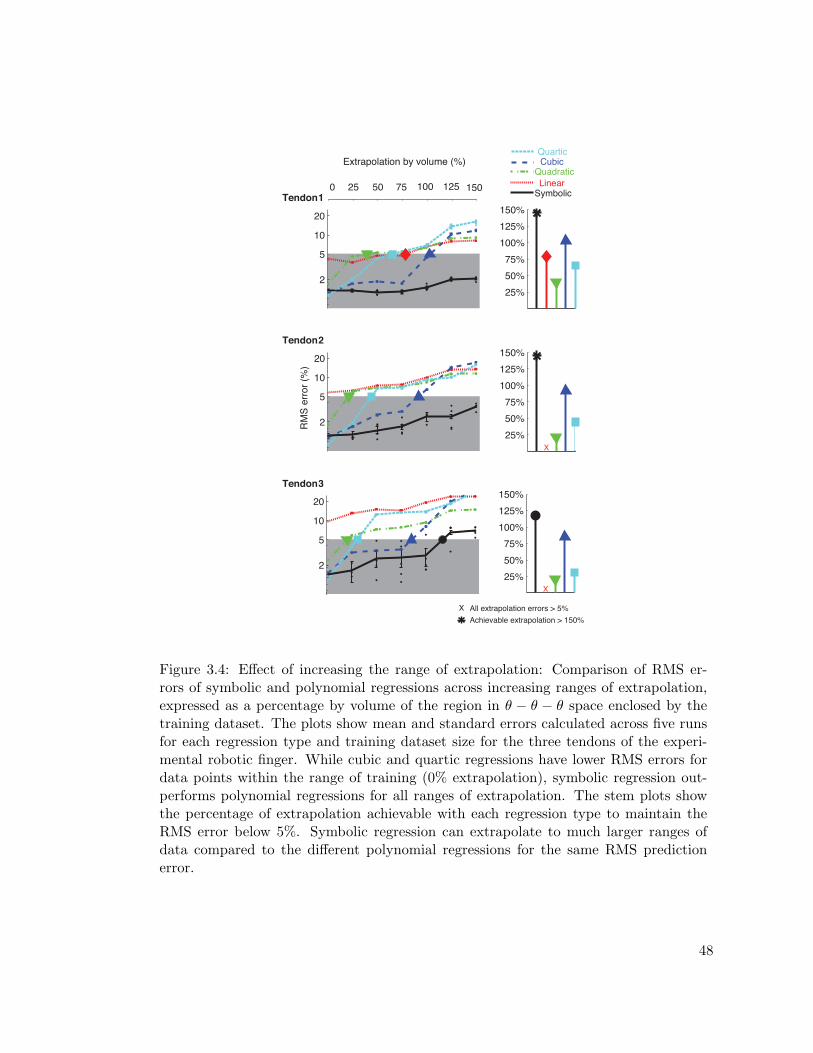
25%50%75%

100%125%150%

Tendon 1

Tendon 2

Tendon 3

RM

S er

ror (

%)

Extrapolation by volume (%)

0 25 15075 10050 125

X

X

X All extrapolation errors > 5%Achievable extrapolation > 150%

2

5

10

20

2

5

10

20

2

5

10

20

25%50%75%

100%125%150%

25%50%75%

100%125%150%

Symbolic

Quartic

LinearQuadratic

Cubic

Figure 3.4: Effect of increasing the range of extrapolation: Comparison of RMS er-rors of symbolic and polynomial regressions across increasing ranges of extrapolation,expressed as a percentage by volume of the region in θ − θ − θ space enclosed by thetraining dataset. The plots show mean and standard errors calculated across five runsfor each regression type and training dataset size for the three tendons of the experi-mental robotic finger. While cubic and quartic regressions have lower RMS errors fordata points within the range of training (0% extrapolation), symbolic regression out-performs polynomial regressions for all ranges of extrapolation. The stem plots showthe percentage of extrapolation achievable with each regression type to maintain theRMS error below 5%. Symbolic regression can extrapolate to much larger ranges ofdata compared to the different polynomial regressions for the same RMS predictionerror.

48

In general, symbolic regression required fewer training data points than polynomial re-

gressions to obtain RMS errors of 5% in tendon excursion predictions (Fig. 3.3). When

tested with the cross-validation dataset, cubic and quartic regressions had lower RMS

errors than symbolic regression for large training dataset sizes, but had much larger er-

rors when the number of training data points was small. However, when tested with

the extrapolation dataset, all polynomial regressions had much larger errors compared

to symbolic regression, independent of the size of the training dataset (Fig. 3.3). These

observations were consistent across all three tendons (S1, S2 and S3 in Fig. 3.1).

3.4.1.2 Effect of Increasing the Range of Extrapolation

Symbolic regression could extrapolate further away from the training datasets compared

to polynomial regressions for the same RMS error in tendon excursion predictions. It

could extrapolate to ranges beyond 150% of the range of the training dataset (by volume)

for tendons one and two and up to 125% for tendon three and still maintain RMS errors

below 5%. In comparison, linear, quadratic and quartic regressions could not extrapolate

beyond 50-75% in most cases, and cubic regression up to 100% for the same RMS error

of 5% in tendon excursion predictions (Fig. 3.4).

Figure 3.5 summarizes the comparison between symbolic and polynomial regressions

for the experimental data from the tendon-driven robotic finger. It shows the achievable

percentage extrapolation for the different regression techniques with reduction in training

dataset size to obtain 5% RMS error in tendon excursion predictions. Symbolic regression

could extrapolate to much larger ranges of data, compared to the polynomial regressions,

for all the training dataset sizes.

49

Extrapolation by volume (%)

0

25

50

75

100

125

150

>150

n n

2n

4n

8n

16n

32n

64n

128

Training set size (n =1688)

Extra

pola

tion

by v

olum

e (%

)

SymbolicQuartic

LinearQuadratic

Cubic

Figure 3.5: Summary of the comparison between symbolic and polynomial regressions intheir ability to extrapolate and their performance with training dataset reduction. Theachievable percentage extrapolation for models trained over different training datasetsizes to maintain RMS errors below 5% is shown for each regression technique for thethree tendons of the planar robotic system. For each training dataset size, symbolicregression can extrapolate to larger ranges beyond the training dataset compared topolynomial regressions.

50

Landsmeer combination Expressions RMS errors (%)

Train. Crossvalid. Ext.

I, I, I Target 1.8θ1 + 1.8θ2 + 1.8θ3Evolved 1.8θ1 + 1.8θ2 + 1.8θ3 0.001 0 0

I, II, III Target 1.8θ1 + 3.6sin(0.5θ2) + 0.6θ3 −(1.6θ3)/tan(0.5θ3) + 3.2

Evolved 1.8θ1 + 3.61sin(0.5θ2) + 1.54θ3−0.778sin(θ3) 0.102 0.084 0.124

I, III, III Target1.8θ1 + 0.6θ3 −(1.6θ3)/tan(0.5θ3) + 0.6θ2 −(1.6θ2)/tan(0.5θ2) + 6.4

Evolved1.8θ1 + 0.61θ3 +1.1θ3tan(0.24θ3) + 0.24θ22 +2.15tan(0.287θ2)

0.007 0.008 0.026

II, II, I Target 3.6sin(0.5θ1) + 3.6sin(0.5θ2) +1.8θ3

Evolved 3.6sin(0.5θ1) + 3.6sin(0.5θ2) +1.8θ3

0.001 0 0

II, II, II Target 3.6sin(0.5θ2) + 3.6sin(0.5θ1) +3.6sin(0.5θ3)

Evolved3.6sin(0.5θ2) + 1.01(θ1 +sin(0.8θ1)) + 1.01(θ3 +sin(0.8θ3))− 0.015

0.043 0.041 0.318

III, II, I Target1.8θ3 + 0.6θ1 −(1.6θ1)/tan(0.5θ1) +3.6sin(0.5θ2) + 3.2

Evolved1.8θ3 + 0.58θ1 + 0.31θ21 −0.06sin(0.43θ21) + θ2 +1.03sin(0.79θ2)

0.031 0.034 0.165

III, III,III

Target

0.6θ1 + 0.6θ2 + 0.6θ3 −(1.6θ1)/tan(0.5θ1) −(1.6θ2)/tan(0.5θ2) −(1.6θ3)/tan(0.5θ3) + 9.6

Evolved

0.58θ1 + 0.58θ2 + 0.55θ3 +0.32θ21 + 0.32θ22 +0.31θ23 − 0.13sin(0.32θ21) −0.13sin(0.32θ22) + 0.018

0.059 0.066 0.345

Table 3.2: Target and inferred expressions with training, cross-validation and extrapo-lation RMS errors(%) for some combinations of Landsmeer’s models I, II, III

51

3.4.2 Results for the Computer-Generated Synthetic Data

All regressions produced very low errors for the computer-generated synthetic data when

no noise or extrapolation was involved. We observed that of the 27 possible combinations

of the three Landsmeer’s models, symbolic regression tended to infer the exact target

ground-truth expressions for joints with models I and II, and found expressions equiva-

lent or closely related to the original expression (e.g., Taylor series terms or alternative

trigonometric forms) for joints with model III (Table 3.2). The training, cross-validation

and extrapolation RMS errors were below 0.4% for all 27 combinations.

3.4.2.1 Robustness to Noise

When experimentally realistic noise was added to the training datasets, cubic and quar-

tic regressions overfit to the noise and performed poorly when tested for cross-validation

and extrapolation (Fig. 3.6). In contrast, symbolic regression outperformed the poly-

nomial regressions for all tendons when tested with extrapolation datasets and matched

quadratic regression when tested with cross-validation datasets. The box plot in Fig 3.6

shows that for the 27 combinations of Landsmeer’s models with noise added, on aver-

age symbolic and quadratic regressions had equivalent cross-validation errors, whereas

symbolic was 8% better than quadratic regression when tested with the extrapolation

dataset. Hence, symbolic regression would be the regression of choice to model tendon

excursions in physiological systems from experimental data, where measurement noise

cannot be avoided.

52

.0

.0001

1

1

Landsmeer combination

Log

RM

S er

ror (

%)

Cro

ss-v

alid

atio

n

9 18 27

50%

Ext

rapo

latio

n

.0001

.01

1

With no noise With noise added

SymbolicQuartic

LinearQuadratic

Cubic

Rat

io R

MS

erro

rs (S

ymbo

lic /

Qua

drat

ic)

9

1

1.1

0.8

0.9

1

1.1

0.

RM

S er

ror (

%)

0.8

1

1.2

1.

2.

9 18 27

2

2

8

Figure 3.6: Comparison of root mean squared errors between symbolic and polynomialregressions for the 27 combinations of Landsmeers models with no noise and with ±5%noise added to joint angles and ±1% to tendon excursions. While cubic and quarticregressions have lower errors than symbolic regression for data with no noise, whenexperimentally realistic noise is added, symbolic regression has much lower errors thanthese polynomial regressions. The box plot on the right shows the ratio of RMS errorsof symbolic to quadratic regression (best among polynomial regressions) for the datawith noise. The median ratio is close to one for cross-validation testing demonstratingthat symbolic and quadratic regressions are equivalent with respect to RMS errors inthis case whereas for extrapolation testing, the median ratio is 0.92 indicating that onaverage, symbolic regression has 8% lower RMS errors than quadratic regression acrossthe 27 models.

53

RM

S er

ror (

%)

Cro

ss-v

alid

atio

nEx

trapo

latio

n

SymbolicQuartic

LinearQuadratic

Cubic

Experimental dataWith no noise

Number of parameters

Simulated dataWith noise added

1

2

3

0 20 401

2

3

5

.0001

.01

1

0 20 40

.0001

.01

1

0 20 401

2

5

10

1

2

5

10

Figure 3.7: Comparison of RMS errors and number of parameters across symbolicand polynomial regression models for experimental data from the three tendons ofthe planar robotic system and synthetic data generated using the 27 combinations ofLandsmeers models with no noise and with experimentally realistic noise added. Inall cases, symbolic regression models have fewer parameters and lower RMS errorscompared to the polynomial regressions.

54

3.4.2.2 Number of Free Parameters as a Practical Measure of the Complexity

of the Analytical Expression

Analytical expressions obtained using symbolic regression had fewer free parameters and

lower cross-validation, extrapolation errors compared to polynomial regressions for ex-

perimental data from the tendon-driven robotic system as well as for the synthetic data

with no noise and with noise added (Fig. 3.7).

3.5 Discussion

We have presented a novel method based on symbolic regression that can infer accurate

analytical expressions mapping joint angles to tendon excursions from sparse datasets.

Symbolic regression outperforms polynomial regression, the state-of-the-art technique

used in musculoskeletal modeling, in that it requires smaller training datasets, can ex-

trapolate to ranges outside that of the training dataset, and does not contain an arbitrary

number of free parameters that can lead to overfitting the training datasets and/or their

noise. We have demonstrated these advantages of symbolic regression using both ex-

perimental and synthetic data and strongly suggest that this approach may be a more

suitable choice to model tendon mechanics for neuromuscular systems.

Obtaining the necessary experimental data to create valid analytical expressions to

represent the musculoskeletal system is invariably difficult and costly. This is true for

both cadaveric specimens and human subjects. Hence it is critical to be able to extract

functionally accurate analytical expressions from as sparse a dataset as possible. More-

over, because the ground truth is not usually known, it is important to have confidence

55

that the expressions found are unaffected by unavoidable measurement noise, that enough

data are available/used, that the form of the analytical expressions is appropriate and

parsimonious, and that the analytical functions are valid for the entire natural workspace

of the limb. We have demonstrated here that symbolic regression, as implemented in Eu-

reqa (Schmidt & Lipson 2009), outperforms polynomial regression, the state-of-the-art in

musculoskeletal modeling, with respect to these performance criteria.

For the physical system of tendons traveling over joints with smoothly varying me-

chanical behavior, it is critical that the tendon excursion expressions model data even

outside the range of the experimentally obtained data points on which they are trained to

ensure they capture the true behavior of the system, and not just overfit to the training

data points. Moreover, obtaining data spanning the entire range of motion of a multi-

degree of freedom biomechanical system is very difficult. It would also necessitate a larger

training dataset. Polynomial models do not extrapolate well again due to their overfit-

ting behavior whereas symbolic regression avoids this problem and can model points well

beyond the range of training data.

Experimental data from biomechanical specimens is unavoidably polluted by measure-

ment noise and/or uncertainty. These can arise from skin deformation, motion capture

errors and/or estimation of axes of joint rotation, measurement errors and/or noise, etc.

Small errors in these measurements lead to large errors in the inferred joint angle kinemat-

ics (Woltring et al. 1983, Cappozzo et al. 1996, Holden et al. 1997). While experimental

data are often filtered, filtering introduces artifacts and reduces the resolution of the mea-

surements. Hence it is important that the regression technique employed be robust to

56

noise and capture the true underlying system behavior with the highest resolution pos-

sible. We show that polynomial regression models, especially higher order polynomials,

overfit to the noise and can be poor representations of the real underlying behavior of

the system. In contrast, symbolic regression is seen to be robust to noise and is more

accurate than polynomial regressions in modeling noisy data.

The form of the analytical function must also strike a balance between parsimony

and accuracy. Functions with a large number of free parameters require a large training

dataset for the estimation of the values of those parameters. They also have a greater

tendency to overfit to the training dataset when compared to models with fewer pa-

rameters. On the other hand, analytical functions with too few parameters will fail to

accurately represent the functional nonlinearities of the system. The symbolic regression

algorithm in Eureqa explores multiple potential forms for the analytical function while

also penalizing the number of parameters; and prioritizes low fitness error solutions with

fewer parameters over those with more parameters. In many of the cases we present,

polynomial functions of higher orders have a large number of free parameters compared

to the more parsimonious analytical functions found by symbolic regression.

The ability of symbolic regression to infer the nonlinear target expressions of the

Landsmeer models shows that our method can capture the underlying physics of the

system directly from input-output data. This is particularly the case here because the

target expressions were derived by Landsmeer by hand using principles of geometry and

anatomy. As argued elsewhere (Schmidt & Lipson 2009), the fact that symbolic regression

did not only infer adequate mathematical expressions but those target expressions is worth

noting. At the very least, this says that those target expressions are parsimonious and

57

that Eureqa is able to favor parsimonious expressions. In addition, this demonstrates how

the analytical expressions for tendon excursions or moment arm variations generated by

symbolic regression may contain insight on the geometry of the tendon routing – and

therefore capture the physics of the system.

Unlike conventional optimization that is based on a ‘single line search’ and finds the

global optimum or one of the local optima of the fitness landscape, Eureqa converges on

a family of optimal solutions that lie on the Pareto front of the fitness error-complexity

plane. The user is then free to choose the solution they want based on the features of the

analytical expressions most important to them such as (i) Observation and knowledge of

the system being modeled, (ii) Fitness error alone, (iii) Cross-validation or extrapolation

error (as we chose to in this chapter), etc. Polynomial regressions or other functional

regressions do not offer this choice. Currently, selection of suitable functions is mostly

driven by the properties and pitfalls of polynomial fitting as opposed to giving the freedom

to the investigator to choose functions for scientific or computational reasons.

Until recently, measuring tendon excursions accurately was only possible in cadaveric

specimens. But with advances in the field of magnetic resonance and ultrasound imaging,

it has become possible to record moment arms in live subjects (Rugg, Gregor, Mandel-

baum & Chiu 1990, Maganaris 2004, Blemker et al. 2007). While in this chapter we have

demonstrated the use of symbolic regression to extract analytical functions mapping joint

angles to tendon excursions assuming direct measurements in cadaveric systems, it will

soon be possible to measure tendon excursions and moment arms non-invasively in vivo

– and our techniques will be applicable to those measurements. This would enable esti-

mation of accurate, subject-specific models of moment arm variation that are critical, for

58

example, in the cases of deformity, surgical modification, injury, or the development of

functional electrical stimulation controllers (Khang & Zajac 1989) and for patient-specific

diagnosis and rehabilitation.

The analytical functions obtained are selected to be computationally efficient for iter-

ative or real-time use, but they can be costly to find off-line. One of the major limitations

of symbolic regression is computational cost, since it uses genetic programming that in-

volves searching a high dimensional space for optimal or near-optimal solutions. Eureqa

was designed to execute on a cluster of parallel computers by automatically parallelizing

the search process, where the computation time is reduced linearly with the number of

processors available. Also, while it might be computationally expensive to infer these an-

alytical expressions, it needs to be done only once. The resulting analytical expressions

can then be used as part of the model in the research of interest. In fact, once inferred, the

computational cost of implementing the expressions is lower given that parsimony (and

therefore computational efficiency) is an explicit fitness criterion. Eureqa’s graphical user

interface allows the user to continuously monitor the fitness error as well as the family

of optimal analytical functions throughout a search. The user can pause and continue,

or terminate the search at any point. In addition, the user has the flexibility to select

the set of mathematical operations that are to be the possible options defining the space

of feasible functions to be generated. While choosing more operations would make the

search more generic and thus increase computational cost for function inference, restrict-

ing the solution space too much can also lead to inappropriate or inaccurate analytical

functions. Hence an informed choice needs to be made based on knowledge of the system

59

being modeled, the purpose of the analytical functions, and availability of computational

power.

State-of-the-art biomechanical modeling involves assuming a fixed topology/form for

the system being modeled and estimating the parameter values from experimental data.

In our previous work (Valero-Cuevas, Anand, Saxena & Lipson 2007), we have demon-

strated that modeling of certain complex biomechanical systems requires simultaneous

inference of both model topology and parameter values directly from experimental data.

Here, as a continuation of that work, we have demonstrated that the conventional method

of assuming a fixed polynomial form and regressing coefficients from experimental data,

suffers from certain drawbacks which can be overcome by using symbolic regression that

simultaneously infers both the form and the parameter values of the analytical expressions

directly from experimental data.

We have demonstrated the advantages of using this method in a tendon-driven robotic

system. We are currently applying it to infer analytical expressions modeling tendon

excursions in the human fingers from cadaveric data.

Acknowledgment

Coauthors Dr. Hod Lipson and Dr. Francisco-Valero-Cuevas. Michael Schmidt for help

with setting up Eureqa. Computation for the work described in this chapter was sup-

ported by the University of Southern California Center for High-Performance Computing

and Communications (www.usc.edu/hpcc). Demelza Gutierrez designed and built the

60

robotic finger. This material is based upon work supported by NSF Grants EFRI-COPN

0836042 and NIH Grants AR050520 and AR052345 to FVC.

61

Chapter 4

Simultaneous Inference of the Form and Parameters of

Analytical Models Describing Tendon Routing in the

Human Fingers.

4.1 Abstract

Control of finger movement and force is made possible by a complex network of tendons.

Analytical models for the excursions and moment arms of these tendons have been used

extensively in the literature to understand finger motion and force, to determine changes

in actions of different muscles with joint posture, and more recently, to model finger

dynamics to test theories of motor control. The analytical models used in the literature are

mostly of two kinds: i. Polynomial regressions and ii. Functions consisting of Landsmeer’s

models which are based on approximate geometry of tendon routing. Both these types

of models assume a fixed form for the mathematical expressions while the parameter

values are either regressed from experimental data or calculated based on assumptions

about the anatomy or some optimization criteria. Here we demonstrate a novel method

based on symbolic regression that simultaneously infers both the mathematical form

62

and the parameter values of these models directly from experimental data. We use this

technique to infer analytical models for the seven tendons controlling the index finger.

We demonstrate that these models are more accurate and have fewer parameters than

both polynomial regressions as well as expressions consisting of Landsmeer’s models when

tested with i. data from multiple trials from the same cadaveric hand and ii. data from

different cadaveric hands. Hence, our symbolic regression approach would be the method

of choice whether the goal is to obtain subject-specific analytical models representing

these systems or models that generalize across the population.

4.2 Introduction

Tendon routing in the human fingers is complex with the presence of networks of inter-

connections that connect multiple muscles to multiple joints. The actuation of these

tendons by the muscles to bring about movement and force is not fully understood

(Zancolli 1979, Brand & Hollister 1999). Computational modeling of these systems have

been extensively used in the literature to understand the role of these networks in human

manipulation including grasp, climbing, playing music (Leijnse 1996, Vigouroux, Quaine,

Labarre-Vila & Moutet 2006, Sancho-Bru et al. 2001, Sancho-Bru, Perez-Gonzalez, Ver-

gara & Giurintano 2003), to understand changes upon injury (Valero-Cuevas et al. 2000),

neuromuscular control(Esteki & Mansour 1996, Valero-Cuevas 2000b) and to develop

functional electrical stimulation controllers (Esteki & Mansour 1997).

Many of these computational models often rely on explicit analytical expressions repre-

senting changes in tendon excursions with joint angles. Instantaneous moment arms (and

63

hence, moment arm matrices) can then be calculated using the tendon excursion-joint

displacement technique (An et al. 1984) by taking partial derivatives of these expressions

with respect to the joint angle changes. Such models have been used in the literature

not only in the fingers but in different musculoskeletal systems in the body, to under-

stand how the action of muscles changes with joint posture (Eg. (An et al. 1983, Spoor

et al. 1990, Herzog & Read 1993, Liu et al. 1997) ). They have been used to validate

anatomical models explicitly representing the physics of interactions of tendons with

bones (Eg. (Murray et al. 1995, Buford Jr et al. 1997)). These analytical models are

particularly important for the simulation of musculoskeletal dynamics to test theories of

motor control where moment arms (part of the system dynamics) need to be evaluated

iteratively several thousand times (Theodorou et al. 2011). In such simulations, com-

pact, simple representations which can be easily differentiated and evaluated quickly are

critical.

The most commonly used analytical models representing tendon routing in the fingers

are based on Landsmeer’s models I, II and III (Landsmeer 1961) where the tendon excur-

sions for the different tendons are represented as combinations of the different Landsmeer

models based on geometry of the joints they actuate. The parameter values for the

Landsmeer models in these cases are obtained from force optimizations in simulation and

ratios of distribution of forces in the different bands of the extensor mechanism (Brook

et al. 1995, Berme, Paul & Purves 1977, Purves & Berme 1980). The other type of

analytical model consists of polynomial regression models where tendon excursions are

assumed to be of polynomial form (linear, quadratic, cubic, etc.) and the coefficients

are regressed from experimental data obtained from cadaveric specimens (Eg. (Franko

64

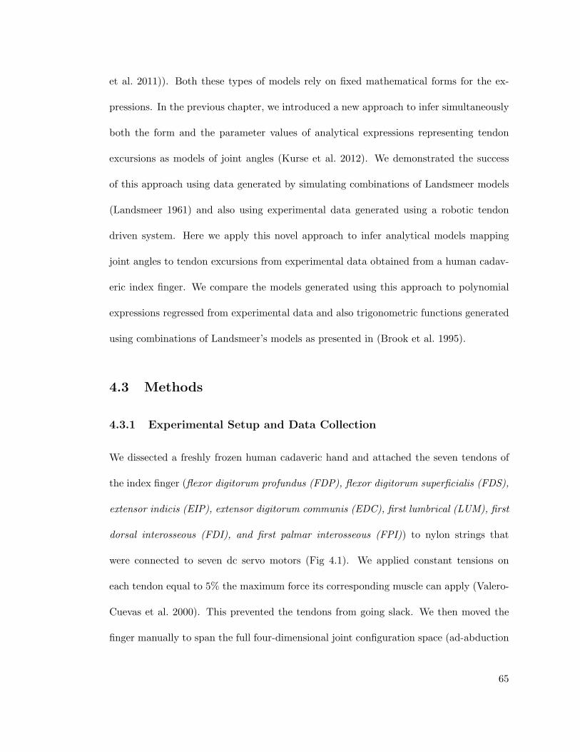
et al. 2011)). Both these types of models rely on fixed mathematical forms for the ex-

pressions. In the previous chapter, we introduced a new approach to infer simultaneously

both the form and the parameter values of analytical expressions representing tendon

excursions as models of joint angles (Kurse et al. 2012). We demonstrated the success

of this approach using data generated by simulating combinations of Landsmeer models

(Landsmeer 1961) and also using experimental data generated using a robotic tendon

driven system. Here we apply this novel approach to infer analytical models mapping

joint angles to tendon excursions from experimental data obtained from a human cadav-

eric index finger. We compare the models generated using this approach to polynomial

expressions regressed from experimental data and also trigonometric functions generated

using combinations of Landsmeer’s models as presented in (Brook et al. 1995).

4.3 Methods

4.3.1 Experimental Setup and Data Collection

We dissected a freshly frozen human cadaveric hand and attached the seven tendons of

the index finger (flexor digitorum profundus (FDP), flexor digitorum superficialis (FDS),

extensor indicis (EIP), extensor digitorum communis (EDC), first lumbrical (LUM), first

dorsal interosseous (FDI), and first palmar interosseous (FPI)) to nylon strings that

were connected to seven dc servo motors (Fig 4.1). We applied constant tensions on

each tendon equal to 5% the maximum force its corresponding muscle can apply (Valero-

Cuevas et al. 2000). This prevented the tendons from going slack. We then moved the

finger manually to span the full four-dimensional joint configuration space (ad-abduction

65

Load cells

Position encodersServo motors

Markers

Figure 4.1: The index finger of a freshly frozen cadaveric finger was moved manuallyto span a range of joint angles. The excursions of the seven tendons were recorded andjoint angles calculated from motion capture data.

66

and flexion-extension at the metacarpophalangeal joint (MCP), and flexion-extension at

the proximal interphalangeal joint (PIP) and the distal interphalangeal joint (DIP) of the

index finger. A single movement trial lasted for five minutes. As we moved the finger,

optical encoders measured tendon excursions at a sampling frequency of 10Hz. We used

a 6-camera optical motion capture system, manufactured by Vicon (Lake Forest, CA),

to track reflective markers adhered to each segment of the finger, at a frequency of 30

Hz. The mean calibration residual error of the marker position reconstruction was less

than 0.2 mm. We processed the 3D coordinates of the markers generated by the Vicon

Nexus software to obtain the four sets of joint angle changes for the entire duration of

movement and then downsampled them to 10 Hz. This provided us a dataset consisting of

a set of joint angles of the four degrees-of-freedom for the index finger and corresponding

tendon excursions of the seven tendons. We divided this complete dataset into a training,

cross-validation and extrapolation datasets. Please see chapter 3 for descriptions of these

datasets. We repeated the movement trial with the same set of tensions on all the tendons

to obtain a second dataset of joint angles and tendon excursions. We also repeated the

above experimental procedure with a second cadaveric index finger to obtain a third

dataset of joint angles and tendon excursions. While we moved the finger to span the full

four-dimensional space in all trials, the actual movement time profiles were different in

each case.

4.3.2 Symbolic Regression Implementation Using Eureqa

We used a software program called Eureqa (Schmidt & Lipson 2009) that implements

symbolic regression using genetic programming to learn the analytical models that map

67

joint angle changes to the tendon excursions of the seven tendons of the index finger.

The objective function defined in the Eureqa environment was to find explicit analytical

models of the form s = f(θ), where s is each tendon’s excursion and θ is the vector of the

four joint angles at every time step, minimizing the root mean squared errors between

predicted and experimentally measured values for tendon excursions (fitness error). Only

the data points from the training dataset were used to infer the analytical models. In

addition to minimizing the error criterion, Eureqa also penalizes model complexity defined

by the number of mathematical operators and parameter values in the function. Using this

multi-objective optimization approach, Eureqa produced a family of multiple ‘optimal’

analytical models (15-20 functions) that map joint angles to the tendon excursions and

lie on the Pareto front of the fitness error vs. complexity (defined above) plane. The

advantage of this approach is that the user now has the choice to pick a solution based

on the criterion of interest: minimizing cross-validation error, extrapolation error or

based on inspection. Please see (Kurse et al. 2012) and Chapter 3 for more details

about Eureqa implementation in tendon driven systems. Here, we chose the expressions

that gave the lowest RMS error when tested on all the data points in the dataset(s)

of interest. On average, we ran each search in parallel for 150 core hours on a cluster

of computers(Dual Dualcore AMD Opteron 2.0 GHz ) at the USC High-Performance

Computing and Communications (www.usc.edu/hpcc) computer cluster.

68

4.3.3 Comparison Against Polynomial Regression and Landsmeer-Based

Models

The state-of-the-art technique in musculoskeletal modeling is to regress tendon excursions

as polynomial functions of joint angles (Eg. (Spoor et al. 1990, Visser et al. 1990, Pigeon

et al. 1996, Liu et al. 1997, Menegaldo et al. 2004, Franko et al. 2011)). We regressed

the coefficients of multivariable linear, quadratic, cubic and quartic polynomials (all cross

terms considered) using MATLAB c© (Version R2009b, MathWorks, Natwick, MA). We

did not consider polynomials of order greater than four because they tend to overfit to the

training data and perform worse than polynomial regressions of lower orders. Spline func-

tions, which are piecewise polynomials stitched together (Murray et al. 1995) would also

overfit to the data. Please see Chapter 3 for more reasoning on why we chose only these

polynomials. We also implemented the analytical models proposed in (Brook et al. 1995)

consisting of combinations of Landsmeer’s models and whose parameter values are based

on force distribution in the extensor mechanism suggested in earlier papers including

(Chao & An 1978a). We uniformly scaled these Landsmeer-based model expressions us-

ing the training dataset to minimize the RMS errors between the experimentally recorded

and model predicted tendon excursions. This was done to account for differences in hand

size across specimens.

While all the analytical models (symbolic, polynomial and Landsmeer-based) were

obtained using only the training data points from the first dataset, they were compared

against each other with respect to i Mean errors across two movement trials from the

69

same cadaveric hand and ii. Mean errors across two trials from two different cadaveric

hands.

4.3.3.1 Two Movement Trials from the Same Cadaveric Specimen

We calculated the RMS errors between model-predicted and experimentally measured

tendon excursions over all the data points in the two datasets from the same cadaveric

specimen. We compared the mean of the two RMS errors for the different analytical

models. In other words, we wanted to see which models had lowest error across the two

datasets. Since symbolic regression gave us a family of multiple analytical models, we

chose the function with the least error across the two datasets for comparison.

4.3.3.2 Two Trials with Two Different Cadaveric Specimens

We repeated the above procedure using : the first dataset (same movement trial used

for training) and the dataset obtained from the second cadaveric specimen. We again

compared the mean of the two RMS errors for the different analytical models to see

which models had the lowest error across the two specimens. For symbolic regression,

we chose the analytical expression with the smallest error among the family of functions

obtained. When testing against data points from the second hand specimen, we scaled

all the models (symbolic, polynomial and Landsmeer-based) uniformly to account for

differences in hand size.

70

sfdp = 10.36θmcp + 10.95θpip + exp(1.84θdip)sfds = 12.47θmcp + 7.22θpip − exp(1.49− 4.22θpip − 24.15θmcpθpip − 26.03θadd)− θdip + 5.34sei = 5.86sin(1.97θadd − θmcp)− 3.92θpip + 0.8sedc = −6.99sin(θmcp − θadd) + 5.09cos(0.23 + θpip)− 4.39slum = 2.54θmcp − 0.71cos(39.7θaddθmcp − 3.1θmcp)− 13.05θadd − 4.83θpip

sfdi = −5.64θadd − 4.4θaddsin(4.94θmcp) + 1.27sin(3.4θmcp) + 1.45cos(1.02 − 1.96θpip) −4.83θaddθpip

sfpi = 9.38θmcp + 9.25sin(3.01θadd)− 11.29θaddθmcp + 4.12cos(θpip + 4.12θadd)− 3.01

Table 4.1: Analytical models obtained using symbolic regression for the excursions ofthe seven tendons of the index finger (FDP,FDS,EIP,EDC,LUM,FDI,FPI) that gener-alize best across trials from the same cadaveric hand.

sfdp = 10.36θmcp + 10.95θpip + exp(1.84θdip)sfds = 12.17θmcp + 8.14θpip − θdip + 4.46sei = −9.61θmcp − 2.85θpip + 1.19sedc = −9.13θmcp + θadd − 3.34θpip + 1.47slum = 2.54θmcp − 13.05θadd − 0.71cos(39.7θaddθmcp − 3.1θmcp)− 4.83θpip

sfdi = 4.51θmcp

sfpi = 9.48θmcp + 8.08sin(2.99θadd)− sin(13.95θaddθmcp) + 4.31cos(θpip + 2.99θadd)− 3.2

Table 4.2: Analytical models obtained using symbolic regression for the excursions ofthe seven tendons of the index finger (FDP,FDS,EIP,EDC,LUM,FDI,FPI) that gener-alize best across trials from different cadaveric hands.

4.4 Results

Table 4.1 shows the ‘best’ analytical models obtained using symbolic regression that had

lowest mean RMS errors across the two movement trials from the same cadaveric speci-

men. These are the expressions that would best describe this specific cadaveric specimen.

The expressions consist mostly of linear, trigonometric and exponential terms. Table

4.2 shows similar analytical models obtained using symbolic regression with lowest mean

RMS errors across the two specimens from among the family of multiple solutions. Note

that both these sets of expressions are from the same family of solutions inferred using

the training data points from the first movement trial. The expressions that generalized

across the two specimens had more linear components, fewer parameters and hence may

be termed simpler than the functions in Table 4.1.

71

FDP FDS EIP EDC LUM FDI FPI2

5

10

20

SymbolicLandsmeer

Quartic

LinearQuadratic

Cubic

Tendon

Nor

mal

ized

RM

S er

ror (

%)

(a) Mean of normalized RMS errors ofthe different models across two move-ment trials from the same cadavericspecimen. The best symbolic regres-sion function (picked from the fam-ily of functions generated) had lowererrors across the two trials comparedto the polynomial regressions and theLandsmeer based models.

2 10 502

5

10

20

50FDP

2 10 502

5

10

20

50FDS

2 10 502

5

10

20

50EIP

2 10 502

5

10

20

50EDC

2 10 502

5

10

20

50LUM

2 10 502

5

10

20

50FDI

2 10 502

5

10

20

50FPI

Number of parameters

(b) Normalized RMS errors vs. the number of parame-ters in the functions generated using the different tech-niques. Symbolic regression expressions had fewer pa-rameters and lower RMS errors compared to the otherfunctions.

Figure 4.2: Comparison of symbolic, polynomial and Landsmeer functions when testedon datasets from two different movement trials from the same cadaveric specimen tocompare generalizability of functions across experimental trials.

72

FDP FDS EIP EDC LUM FDI FPI2

5

10

20

Tendon

Nor

mal

ized

RM

S er

ror (

%)

SymbolicLandsmeer

Quartic

LinearQuadratic

Cubic

(a) Mean of normalized RMS errorsof the different regressions across twomovement trials from two different ca-daveric specimens. The models wereall trained on dataset from one speci-men but uniformly scaled when testedon the other specimen. The best sym-bolic regression model (picked fromthe family of functions generated) hadlower mean errors across the speci-mens, compared to the other func-tions.

2 10 502

5

10

20

50FDP

2 10 502

5

10

20

50FDS

2 10 502

5

10

20

50EIP

2 10 502

5

10

20

50EDC

2 10 502

5

10

20

50LUM

2 10 502

5

10

20

50FDI

2 10 502

5

10

20

50FPI

Number of parameters

(b) Normalized RMS errors vs. the number of param-eters in the models generated using the different tech-niques. Symbolic regression expressions had fewer pa-rameters and lower RMS errors compared to the othermodels.

Figure 4.3: Comparison of symbolic, polynomial and Landsmeer models when tested ondatasets from two different cadaveric specimens to compare generalizability of modelsacross hands.

73

Fig. 4.2(a) shows the comparison of performance of the analytical models for symbolic

regression against other analytical models upon testing with data points from the two

movement trials from the same cadaveric hand. The symbolic regression functions had the

lowest RMS errors. While the errors for the flexor tendons (FDP, FDS) were comparable

across the different models, the models had more varying errors for the extensor (EIP,

EDC) and intrinsic tendons (LUM, FDI, FPI). The intrinsic tendons also had much larger

errors compared to the other tendons. Quartic regression in all cases had very large errors.

Quartic regression tends to overfit to the training data points and has been observed to

perform badly with cross-validation and extrapolation data 3.

Fig. 4.2(b) shows the RMS errors of the models vs. the number of parameters in

each. Expressions with fewer parameters may be considered simple, have lesser tendency

to overfit to the data and hence, are more desirable. Symbolic regression expressions had

lower RMS errors as well as fewer parameters than the other models.

Fig. 4.3(a) shows the comparison of the different models when tested with data

points from two different specimens. The errors for all models were larger than before

as expected. Symbolic regression solutions again had lower errors than the other models

(except for the FDI where cubic regression model had a lower RMS error). The mod-

els disagree much more in this case with respect to one another for all the tendons in

comparison to the previous case. The intrinsic tendons (LUM, FDI, FPI) were observed

to have larger errors in all models in comparison to the extrinsic tendons (FDP,FDS,

EIP and EDC). Fig. 4.3(b) compares the RMS errors of the models vs. the number of

parameters. Symbolic regression expressions had fewer parameters and lower errors than

the other models.

74

4.5 Discussion

We have implemented a novel method based on symbolic regression to simultaneously

infer the mathematical form and parameter values of analytical models representing the

tendon excursions of the index finger. We have demonstrated that these models are more

accurate than both polynomial regressions (linear, quadratic, cubic and quartic) as well

as Landsmeer-based models in representing tendon routing, whether our goal is to obtain

i. subject-specific models of these systems or ii. models that generalize across specimens.

We also show that these symbolic regression models have fewer parameters than the other

models which is important to ensure they do not overfit to the training data points.

The analytical models obtained using symbolic regression that best fit the data from

a single cadaveric hand mostly consisted of linear, exponential and trigonometric com-

ponents. The expressions for the tendon excursions give some insight into the physics

of interaction and routing of these tendons. For example, the expressions for the lum-

brical and the FPI contain coupling terms θmcpθadd reflecting on the way these tendons

are routed about the MCP joint whereas tendons like the FDP and FDS do not contain

this term and are known to produce a more straightforward flexion-extension motion at

the joints. This insight is not available in case of polynomial regressions. The analytical

models that generalize well across the two hand specimens are ‘simpler’ than the func-

tions in the previous case with the latter consisting of a larger number of linear terms.

While we know that these functions generalize best across the two cadaveric specimens

in comparison to the other models, whether they are sufficiently accurate would have to

75

be decided by the modeler looking at the RMS error values presented in Fig. 4.3(a) and

the problem they are trying to solve.

As we have shown in chapter 3, polynomial regressions tend to overfit to the training

dataset. This results in very large errors when tested on data points either not in the

training dataset but lying in the range of the training data (cross-validation dataset) or

data points outside the range of training (extrapolation dataset). Hence when tested on

the complete dataset as we have done here, the errors of functions like quartic regression

are very high.

All models are more accurate for the ‘simpler’ tendons, the FDP, FDS, EIP and EDC,

in comparison to the intrinsic muscles (LUM, FDI, FPI). These larger errors could be at-

tributed in part to the joint model of the MCP where the orientation of the ad-abduciton

axis to the flexion-extension axis has been long debated (Berme et al. 1977, Youm, Gille-

spie, Flatt & Sprague 1978, Valero-Cuevas 1997) and in part because these tendons do not

independently control the finger joints but attach to the extensor mechanism which in turn

controls joint motion. Again the complexity of the extensor mechanism is well known (Eg.

(Landsmeer 1949, Garcia-Elias, An, Berglund, Linscheid, Cooney Iii & Chao 1991),etc.).

Also, there have been variations observed across the population in terms of attachment

points of the intrinsic muscles (Salsbury 1937). This could also explain why all models

performed much worse for the intrinsics when tested across datasets from two different

hand specimens.

Models with fewer coefficients are preferable to models with a large number of coeffi-

cients to reduce overfitting (Kurse et al. 2012). They may also be considered as ‘simpler’

and more elegant representations of the system. Symbolic regression functions had much

76

fewer parameters than the other models. This is because Eureqa (the symbolic regression

program used here) explicitly favors solutions that have fewer mathematical components

(parameters and mathematical operators) to those with a larger number of mathematical

components.

Most existing studies use cadaveric testing to obtain analytical models for moment

arms and tendon excursions. But, with advances in imaging, it is becoming possible to

measure tendon excursions and moment arms in live subjects(Rugg et al. 1990, Maganaris

2004, Blemker et al. 2007). We can then apply our methodology to datasets from these

imaging studies to obtain accurate, subject-specific models of tendon routing that would

be critical to developing functional electrical stimulators or for diagnosis and repair.

While the analytical models obtained using symbolic regression are selected to be com-

putationally efficient for iterative or real-time use, they can be computationally expensive

to find. But this needs to be done only once. Please see Chapter 3 for the limitations of

Eureqa and how some features built in Eureqa help to minimize those limitations.

Acknowledgment

Coauthors Dr. Hod Lipson and Dr. Francisco-Valero-Cuevas. Dr. Marta Covadonga

Mora Aguilar and Dr. Jason J. Kutch for helping me with the cadaver experiments. I

would also like to thank the hand surgeons, Dr. Vincent Hentz, Dr. Caroline Leclercq, Dr.

Isabella Fassola and Dr. Nina Lightdale for doing the cadaveric dissections. Computation

for the work described in this chapter was supported by the University of Southern Califor-

nia Center for High-Performance Computing and Communications (www.usc.edu/hpcc).This

77

material is based upon work supported by NSF Grants EFRI-COPN 0836042 and NIH

Grants AR050520 and AR052345 to FVC.

78

Chapter 5

Experimental Cadaveric Actuation Gives Insight on

Control of Human Finger Movement

5.1 Abstract

Human finger movement is produced by the coordinated actuation of several tendons

interacting with one another. The control mechanisms that produce this movement are

not well understood. In this chapter, we describe the use of computer controlled servo

motors to actuate the seven tendons of a cadaveric index finger to produce a simple

tapping motion. We observe that controlling the motors as tunable springs, similar to

human muscles, is an effective way to control finger movement in comparison to simple

force or position control. We also observe that two types of equilibria can be demonstrated

in the cadaveric finger: i. stable equilibrium where the displacement of the finger brings

it back to a specific posture and ii. what we describe as neutral equilibrium observed in

a specific range of postures and tendon tensions where the finger when disturbed from

equilibrium stays in the new displaced posture. We show that the tendon tensions in the

79

latter type of equilibrium lie close to the null space of the moment arm matrix that maps

tendon tensions to joint torques.

5.2 Introduction

Slow and accurate finger movements are critical to human manipulation. There have

been several studies in the literature that have described these movements in different

activities of daily living, like typing, movement to grasp, etc (Eg. (Dennerlein, Mote Jr &

Rempel 1998, Santello, Flanders & Soechting 2002)). But how the nervous system controls

the complex musculature that actuates the human fingers to produce these movements

is not completely understood. Understanding control of finger movement is important to

be able to predict and correct changes that happen during injury and disease, to develop

functional electrical stimulation controllers and to build better robotic and prosthetic

hands.

Accurate measurement of the excursions of the tendons actuating the fingers and the

corresponding muscle forces during these simple finger movements would give insight on

how the nervous system is controlling them. Unfortunately, it is currently impossible to

measure both forces and tendon excursions accurately in a live person. While electromyo-

graphy (EMG) is useful to determine when a particular muscle or groups of muscles are

turning on and off, how the signal can be related to either muscle force or tendon excur-

sions is not clearly understood (Inman, Ralston, De CM Saunders, Bertram Feinstein &

Wright Jr 1952, Disselhorst-Klug, Schmitz-Rode & Rau 2009). On the other hand, arti-

ficially actuating a human cadaveric specimen makes it possible to completely measure

80

inputs (the tendon excursions and forces) and outputs (fingertip forces and joint angle

changes). In this chapter we describe the cadaveric actuation system we have developed,

that enables us to selectively control the tendons of a human cadaveric hand. We use

this setup to control the tendons of the index finger to produce a slow tapping motion

(flexion-extension movement) and to study finger equilibrium at different postures and

input tendon tensions. This cadaveric actuation gives us a better understanding of the

problems the nervous system faces when actuating the complex musculature of the fingers.

5.3 Methods

We dissected a freshly frozen human cadaveric hand and mounted it on a fixed support

using an external fixator (Agee-WristJack, Hand Biomechanics Lab, Inc., Sacramento,

CA). We attached the seven tendons of the index finger (flexor digitorum profundus

(FDP), flexor digitorum superficialis (FDS), extensor indicis (EI), extensor digitorum

communis (EDC), first lumbrical (LUM), first dorsal interosseous (FDI), and first palmar

interosseous (FPI)) to nylon strings that were connected to seven dc servo motors (Fig.

5.1). We measured the tension exerted on each tendon using one degree-of-freedom load

cells and the tendon excursions using optical encoders attached to the motors. We used a

real-time controller (PXI 8108, National Instruments, Austin, TX) to control the motors

in three different modes : i. position control mode where the motors were commanded to

apply specific tendon excursions on each of the tendons, ii. force control mode where the

motors were commanded to apply specific tension on each tendon, and iii. sping control

mode where the motors were made to behave like tunable springs whose spring constant

81

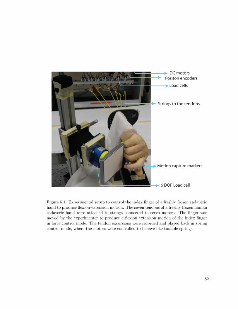
Load cells

Strings to the tendons

Motion capture markers

6 DOF Load cell

DC motorsPositon encoders

Figure 5.1: Experimental setup to control the index finger of a freshly frozen cadaverichand to produce flexion-extension motion. The seven tendons of a freshly frozen humancadaveric hand were attached to strings connected to servo motors. The finger wasmoved by the experimenter to produce a flexion extension motion of the index fingerin force control mode. The tendon excursions were recorded and played back in springcontrol mode, where the motors were controlled to behave like tunable springs.

82

could be adjusted and the command to each motor was in the form of change in resting

length of the spring.

5.3.1 Control of Finger Tapping Motion

The first phase of the experiment was the recording phase. In this phase, we maintained

a constant tension of 5N on all the tendons of the cadaveric finger using force control

mode and moved the finger manually to produce a motion that resembled a simple finger

tap (Venkadesan & Valero-Cuevas 2008). We recorded tendon tensions and excursions

throughout the movement. The next phase of the experiment was the playback phase

where we played back the excursions recorded in the first phase as changes in resting

lengths of the tunable springs corresponding to each tendon in spring control mode. This

helped us to replicate the tapping motion produced in the first phase.

5.3.2 Finger Equilibrium Study

We applied a constant tension of 3N to each of the seven tendons of the index finger

in force control mode (coordination pattern 1). The finger came to a stable equilibrium

position. We then perturbed the finger by displacing it from this position and the finger

returned to the equilibrium posture. Then, keeping the finger in a specific posture (neutral

ad-abduction and approximately 20 degrees flexion at the metacarpophalangeal (MCP),

proximal interphalangeal (PIP) and distal interphalangeal (DIP) joints), we adjusted the

tensions on the tendons by trial and error to find a specific set of tensions that maintained

the finger in that posture in equilibrium (coordination pattern 2). We then moved the

finger to a different posture keeping the tension on each of the tendons the same (using

83

6 DOF loadcell

Load cells measur-ing tendon tensions

Strings connecting tendons to motors

Fingertip force vector

Figure 5.2: The experimental setup used to record fingertip forces from a freshly frozencadaveric hand. We applied all possible combinations of high and low tensions tothe seven tendons of the index finger (there are 128 such combinations) and recordedcorresponding fingertip forces. We repeated this in three different finger postures : fullyflexed, tap and fully extended.

84

force control) and the finger stayed in equilibrium even in the new posture. We observed

a range of finger postures where the finger remained in this equilibrium. We call this state

of equilibrium, neutral equilibrium and describe more in section 5.5. Movement beyond

this range resulted in the finger attaining the posture that formed the boundary of this

neutral equilibrium. We then increased the tension on one of the finger tendons (FDS)

(coordination pattern 3) and this neutral equilibrium was lost. The finger now reached

a new equilibrium, in a new posture. Changing the finger posture manually resulted in

the finger coming back to this new equilibrium in a spring like behavior.

We then performed an isometric force production experiment where we adjusted the

finger segments to a posture in the range where the neutral and stable equilibrium had

been observed in the previous scenario, and attached the cadaver fingertip to a six degree-

of-freedom load cell (Fig. 5.3). We applied multiple combinations of tendon tensions

consisting of a low force of 1N and high force of 11N (using force control mode) and

recorded the corresponding fingertip forces. We then regressed a matrix mapping tendon

tensions (Fm) to fingertip force (Ftip) which we call the action matrix (A). We then

multiplied this matrix with the transpose of the jacobian (J(θ)) transforming joint angle

velocities to fingertip velocities, to obtain the moment arm matrix (R) of the finger in

this posture. We did not use the entire fingertip wrench (force and torque at the endpoint

(Valero-Cuevas et al. 1998)) but only the fingertip force. Hence the action matrix is only

an approximation of the actual action matrix. Below is the mathematical derivation of

the moment arm matrix.

85

It can be shown using Principle of Virtual Work (Yoshikawa 1990, Valero-Cuevas

2009),

Ftip = J(θ)−Tτ

where Ftip is the wrench vector at the fingertip, J(θ)) is the Jacobian transforming joint

angle velocities to fingertip velocity and the τ is the vector of joint torques. However,

τ = RFm

where R is the moment arm matrix and Fm is the vector of tendon tensions. Hence,

Ftip = J(θ)−TRFm

Ftip = AFm

A = J(θ)−TR

R = J(θ)TA

We then calculated joint torques (τ = RFm) using the moment arm matrix R. The

null space of the 4× 7 moment arm matrix is 3 dimensional. We calculated the distance

of the three coordination pattern vectors from the null space of the moment arm matrix

to see how far each of these patterns were from being in the null space. Here is how we

determined the distance from the null space:

w = U(UT (U))−1UTFm

86

d = ‖Fm −w‖

where U is the matrix formed by the bases vectors of the null space of the action matrix

A and w is the projection of Fm on the null space.

5.4 Results

We were able to successfully control the motion of the human cadaveric finger and record

tendon excursions and tendon tensions for all movements.

5.4.1 Results from Control of Finger Tapping Motion

Fig. 5.3 shows the start and end posture of the cadaveric finger during the tapping

motion as well as the time history of excursions and tensions of the seven tendons. The

playback of the finger tapping motion using the spring control mode produced smooth,

repeatable movements at all the joints. Even though the motion produced was a simple

flexion-extension, a coordinated set of excursions of all tendons were required. This is

due to the routing of the seven tendons around the four degrees-of-freedom of the index

finger. The tension profiles observed were based on the spring stiffness chosen to produce

the movement and are not unique.

5.4.2 Results from Finger Equilibrium Study

We observed that the finger exhibited two kinds of equilibria when the tendons were held

at constant tension in force control mode: i. Stable equilibrium where the displacement

of the finger posture resulted in its coming back to the same posture, and ii. what

87

Tendon Excursions (mm) Tendon Tensions (N)

0 205 410−15

0

15

0 205

0

5

10 FDPFDSEIEDCLUMFDIFPI

Figure 5.3: Tendon excursions and tendon tensions for a single tap. The figure showsthe cadaver finger in the start and end of a single tap. Even a simple flexion-extensionmotion of the finger requires a coordinated set of excursions of all the seven tendonscontrolling the index finger. The tendon tension profile shows the tensions in thecorresponding tendons during this movement which are not unique.

88

FDP

FDS

EI EDC

LUM

FDI

FPI

1 2 30

0.05

0.1

0.15

0.2

0.25

Sum

of j

oint

torq

ues

(Nm

)

1 2 30

1

2

3

4D

ista

nce

from

nul

l spa

ce (N

)

1 2 3

0

2

4

6

8Te

ndon

tens

ions

i

ii iii

FDP

FDS

EI EDC

LUM

FDI

FPI

FDP

FDS

EI EDC

LUM

FDI

FPI

Coordination pattern

Change in tension in single tendon

FlexorsExtensorsIntrinsics

Figure 5.4: Results from the finger equilibrium study. i. Three different coordinationpatterns were applied to the seven tendons. The only difference between coordinationpattern 2 and 3 is the tension applied to the FDS tendon. ii. The sum of jointtorques was calculated for each of the three coordination patterns based on a constantmoment arm matrix regressed from experimental data consisting of tendon tensions andfingertip force outputs in an isometric test. The calculated joint torque was smallestfor the second coordination pattern that produced neutral equilibrium in the finger.iii. Calculating the distance of the coordination patterns from the null space of themoment arm matrix showed that the second pattern producing the neutral equilibriumwas closest to the null space.

89

we describe as neutral equilibrium where the displacement of the finger results in a new

posture and the finger stays in equilibrium in this new posture. In section 5.5, we describe

how we believe these equilibria are being attained.

Fig 5.4 shows the three coordination patterns applied and the results from the calcu-

lation of the joint torques and distances from the null space. The sum of joint torques in

the four-degrees of freedom was smallest in coordination pattern 2 compared to the other

two coordination patterns. The distance of coordination pattern 2 from the null space

of the moment arm matrix was also the smallest, implying that coordination pattern 2

which produced the neutral equilibrium pattern in the finger was closest to the null space

of the moment arm matrix among the three patterns.

5.5 Discussion

We have demonstrated the successful control of a cadaveric index finger to produce a

simple tapping motion consisting of flexion-extension of the MCP, PIP and DIP of the

index finger. We have also demonstrated that the finger exhibits neutral equilibrium in a

specific range of joint postures and tendon tension combinations and stable equilibrium

in others, when the tendon tensions are maintained at a constant set of values.

Even a simple motion like finger flexion-extension requires a coordinated set of tendon

excursions in all the tendons. But this does not necessarily mean that all the muscles

attached to these tendons need to be activated. Muscles not activated would be stretched

passively by the actions of the other muscles and the joint motion. The tendon tension

profile we recorded in our cadaveric actuation setup is again the force that in a living

90

person would come from both active contraction and passive stretching. These force

profiles are not unique due to redundancy in the system (Bernstein 1967, Kutch & Valero-

Cuevas 2011). Multiple sets of muscle forces can lead to the same tendon excursions and

joint motion. The nervous system could pick a coordination pattern depending on the

task and the cost function being considered.

We tried to implement the finger tapping motion in force control, position control and

spring control modes. Force control, where the command consists of specific sets of tendon

tensions, requires a very accurate model of the plant. Otherwise the specimen could be

damaged if a specific force is being commanded on a tendon that cannot be produced due

to kinematic restrictions or action of other muscles. Simple position control again requires

a perfect model of the plant to avoid tendons from going slack. Also demanding a specific

set of tendon excursions could result in very high tendon tensions resulting in the system

getting locked leading to damage. The spring based control where inaccuracies in the

model of the plant are accounted for by simulated passive compliance in the controller

proved most effective in the control of the index finger. The spring based control is

analogous to the working of muscles in the human system. Command from the alpha

motor neuron can be considered as a command that reduces the resting length of a spring

resulting in force being generated. The force-length and force-velocity properties of the

muscle would effectively change the stiffness of this viscoelastic structure. Together the

finger can be considered to being displaced from one equilibrium position to another. See

Section 5.7 for a simulation study discussing this in more detail.

Joint equilibrium upon loading of tendons has been discussed with respect to the

fingers and also other joints in the body(Landsmeer 1961, Zdravkovic, Jacob & Sennwald

91

1995). But, to the best of our knowledge, equilibria of finger joints at different tendon

tension combinations and joint postures has not been studied experimentally in cadaveric

specimens. Our cadaveric setup allowed us to tune in different tendon tensions easily and

observe changes in different postures. We observed both stable equilibrium discussed in

the literature before (Landsmeer 1961) where the finger upon external perturbation to

posture returned to a specific posture, as well as neutral equilibrium where the finger

upon displacement stayed in the new posture.

There is a natural equilibrium of the finger that is stable : produced by the stiffness

created by the skin, the ligaments, etc. This stiffness is larger at the boundaries in

comparison to the working range of the finger (Esteki & Mansour 1996). When perturbed

with no tendon tension inputs, the finger comes to an equilibrium posture. When a control

input is applied in the form of joint torque produced by tendon forces, then depending

on the tendon tension pattern, different behavior is observed: i. If the tendon tension

profile is in the null space of the moment arm matrix of the finger (in that posture),

the finger exhibits ‘neutral equilibrium’ where any perturbation in posture results in the

finger staying in this new posture because the equilibrium conditions are satisfied in this

new posture. This kind of behavior is seen in the working range of the finger motion

where the torque due to ligaments, skin, etc. is very small compared to the torque

produced by tendon tension. ii. For tendon tension profiles that do not lie in the null

space of the moment arm matrix, the equilibrium posture is closer to the boundaries of

the range of finger motion where the torque due to the passive stiffness (skin, ligaments,

etc.) balances the torque produced by the tendon tensions. See the Appendix (Section

5.6) for a mathematical description of this equilibrium.

92

When calculating the moment arm matrix, we only considered the fingertip force

output and not the torque that the four degree-of-freedom finger produces at the fingertip

(Valero-Cuevas 2009). We need to include the measured fingertip torque when regressing

the action matrix from finger output and tendon tensions. It is possible that the sum of

torques at the joints as well as the distance from the null space would be much smaller

than that calculated here if this fingertip torque were included in the analysis.

In this study the tendons were being held at a constant tendon tension pattern (using

force control). This is not exactly true in the human system, since changes in posture

result in changes in muscle lengths and hence, in tendon tensions (force-length relation-

ship). However, for small finger movements the length changes of the muscles would be

relatively small and hence keeping the tension profile also relatively fixed.

The existence of neutral equilibrium could be used by the central nervous system in

finger grasp. While the nervous system sends a simple finger flexion command, the finger

posture would be adjusted based on the shape of the object being grasped. Experiments

with EMG recordings in live subjects from the finger muscles during grasp would need

to be performed to test if this is true.

Acknowledgment

Coauthors Dr. Francisco Valero-Cuevas and Dr. Jason Kutch. The hand surgeons, Dr.

Vincent Hentz, Dr. Caroline Leclercq, Dr. Isabella Fassola and Dr. Nina Lightdale for

doing the cadaveric dissections. Dr. Jae Woong Yi for building the cadaver actuation

93

setup. NSF Grants EFRI-COPN 0836042 and NIH Grants AR050520 and AR052345 to

FVC.

5.6 Appendix: Mathematical Explanation of Finger Equilibria

We describe here in more detail using a dynamical systems perspective, the two states of

equilibria of the finger. The finger can be described as a second order dynamical system.

Then the equation of motion of the system would be:

Iθ + Cθ +Kθ = τ

where I is the moment of inertia of the finger, θ represents the vector of joint angles at

the four degrees of freedom in the finger, C is the viscosity coefficient, K is the stiffness

coefficient and τ is the vector of joint torques produced by the tendons. Suppose the

states of the system are x1,x2 where x1 = θ and x2 = θ

x1 = x2

x2 = θ = I−1(τ −Kθ − Cθ)

In equilibrium,

x1 = 0

x2 = 0

94

which implies,

θ = 0

I−1(τ −Kθ − Cθ) = 0

I−1(τ −Kθ) = 0

(τ −Kθ) = 0

But,

τ = RFm

RFm −Kθ = 0

But in the central region of the workspace of the finger, K is negligible compared to RFm.

Hence, if Fm lies in the null space of R, then there is ‘neutral equilibrium’. And when

it is not in the null space of R, then there is a net torque at the joints which displaces

the finger till it reaches the boundary where the K is not negligible. The new equilibrium

then corresponds to a posture, θ such that RFm −Kθ = 0.

95

5.7 Appendix: A Strain-Energy Approach to Simulating

Slow Finger Movements and Changes Due to Loss of

Musculature

5.7.1 Introduction

The neuromuscular interactions that produce slow and accurate finger movements are

not understood. The geometry of finger anatomy is such that a slow finger movement

(i.e., sequence of joint rotations) completely defines the necessary excursions of all ten-

dons. Given that muscle tone prevents tendons from becoming slack, all tendons must

undergo eccentric or concentric excursions during functional finger movements. Here, we

describe a novel computational solver to model slow finger movements, and report how

the mathematics of strain-energy of over-constrained systems can predict the impairment

in finger motion that accompanies partial paralyses.

5.7.2 Methods

A slow moving finger is best modeled as a first order dynamical system having low mass

and performing quasi-static motion (which is not the case for fast finger movements

(Darling et al. 1994)). Our 3-D model consists of a kinematic 3-link mechanism with

2 degrees of freedom (ad-abduction and flexion-extension) at the metacarpophalangeal

joint (MCP) and 1 degree of freedom (flexion-extension) at the proximal interphalangeal

(PIP) and the distal interphalangeal (DIP) joints. All seven muscles of the index finger

were included: flexor digitorum profundus (FDP), flexor digitorum superficialis (FDS),

extensor indicis proprius (EIP), extensor digitorum communis (EDC), first lumbrical

96

(LUM), first dorsal interosseous (FDI), and first palmar interosseous (FPI). The routing

of the tendons across finger joints is represented by the moment arm matrix obtained

from (An et al. 1983). Our focus here is the computational engine, thus for now we

have neglected the extensor mechanism, but its effects will be considered in subsequent

work. Torsional springs at the joints simulate the known passive stiffness arising from

skin and soft tissue. The muscles actuating the index finger are modeled as tunable linear

elastic springs that only exert force in tension. Changing the latent resting length of a

spring, l0 , results in a muscle force that is proportional to the difference between its

current and resting lengths. Therefore the activation signal to a muscle is simulated as

a change in resting length, ∆l0 (Fig. 1). Here, we are only interested in understanding

how finger movement arises from ∆l0 , and simply assume that ∆l0 can arise from a

neural command. A set of commanded resting lengths to all muscles defines the posture

attained by minimizing the strain-energy of the finger at equilibrium: where the net joint

torques produced by the muscles, τ ext , are exactly balanced by the torques produced by

joint-stiffness,τ in .

∆s = RT (∆θ)

τ ext = RKm(∆l0 −∆s)

τ in = Kθ(∆θ)

97

where ∆s is the change in tendon excursions, R is the moment arm matrix, Km is the

matrix of muscle spring constants,∆l0 is the change in spring resting lengths, Kθ is the

matrix of torsion spring constants at the joints and ∆θ is the resulting change in joint

angles.

Given that muscles behave like nonlinear springs that do not exert compressive force,

there is an extra constraint defined by,

Km ≈ 0 if ∆l0 < RT∆θ (5.1)

Also, we ensure that ∆l0 > 0 since muscle activation always leads to a net force

greater than passive stretch force. We solve the forward kinematic problem iteratively

using a Newton-Raphson iteration method.

As a first demonstration of our system, we simulated a simple quasi-static tapping

motion by finding an appropriate trajectory of muscle resting length changes. The move-

ment consisted of an initial retraction of the index finger followed by a downward flexion

motion (Fig. 5.5). In addition, we simulated the resulting trajectory for acute radial,

median and ulnar nerve palsies by removing the muscle commands to the i) two extensors,

ii) the two flexors, and iii) the two interosseii and lumbrical, respectively and applying

the same resting length change commands as before to the unaffected muscles. This sim-

ulates effects prior to neuromuscular adaptation (i.e., the robustness of finger trajectories

to acute loss of some muscles). Note that the affected muscles continue to exert passive

stretch forces even without the activation command.

98

All intactRadial nerve palsyMedian nerve palsyUlnar nerve palsy

Figure 5.5: Fingertip trajectories for a simple tapping motion in unaffected and im-paired cases.

99

5.7.3 Results and Discussion

Not surprisingly, the fingertip deviates from the original trajectory when some muscle

commands are removed (Fig. 5.5). Some postures and directions of movement become

impossible without the presence of specific muscles. However, the value of these simula-

tions is that they begin to explain the relative effect of different deficits and indicate which

muscles are more or less critical to the execution of accurate and slow finger movements.

In addition, finger movements are typically modeled using second order dynamics(Sueda

et al. 2008, Venkadesan & Valero-Cuevas 2008). Here we are proposing that a simple

quasi-static solver based on strain-energy equilibrium can model slow finger movements

since mass and inertia properties of fingers are small. While muscle mechanics depends

on neural activation and a muscles force-length and force-velocity properties, the end

product is a force command, which we generate by the adjustment of resting lengths of

fictitious springs.

100

Chapter 6

Experimental Validation of Existing Models of the Index

Finger

6.1 Introduction

The role of the different components of the extensor mechanism in finger function has

been long debated in the literature. While several simplistic computational models have

been suggested over the years, the normative model developed by An et al. 1979 (Chao &

An 1978a, An et al. 1979) remains the most comprehensive 3D anatomical model of the

index finger to date. Though this model has been employed in several research studies

(Eg. (Harding et al. 1993)), it has never been rigorously validated with experimental

data. The model assumes bowstringing of all tendons with joint rotation and a constant

force distribution within the different bands of the extensor mechanism, independent of

joint posture. Both the above assumptions are modeling simplifications and are contrary

to experimental observations. Valero-Cuevas et al. in 1998 (Valero-Cuevas et al. 1998)

emphasized the importance of including changes in force distribution through the extensor

mechanism, with finger posture. They modified a constant moment arm model proposed

101

by An et al, 1983 (An et al. 1983), obtained by regression of tendon excursion-joint

angle data from cadaveric specimens, to include changes in force distribution through the

extensor mechanism with posture. But the validity of fingertip force predictions of neither

of these models has been tested with experimental data. In this chapter, we rigorously

validate the normative model of the index finger as well as the constant moment arm

models described in An et al, 1983 and Valero-Cuevas et al. 1998, with experimental

data collected from a cadaveric index finger in multiple postures.

6 DOF loadcell

Load cells measur-ing tendon tensions

Strings connecting tendons to motors

Fingertip force vector

Figure 6.1: The experimental setup used to record fingertip forces from a freshly frozencadaveric hand. We applied all possible combinations of high and low tensions tothe seven tendons of the index finger (there are 128 such combinations) and recordedcorresponding fingertip forces. We repeated this in three different finger postures : fullyflexed, tap and fully extended.

102

6.2 Methods

The seven tendons of the index finger: flexor digitorum profundus (FDP), flexor digito-

rum superficialis (FDS), extensor indicis (EI), extensor digitorum communis (EDC), first

lumbrical (LUM), first dorsal interosseous (FDI), and first palmar interosseous (FPI), in

a freshly frozen cadaveric hand were actuated using dc motors controlled by a National

Instruments PXI real-time control system (Fig. 6.1). All possible combinations of low

(2N) and high (10N) tendon tensions were applied to the cadaveric specimen and corre-

sponding fingertip forces and torques were recorded using a 6 DOF load cell attached to

the fingertip. This procedure was repeated at three different postures in one cadaveric

specimen.

A matrix transforming tendon tensions to fingertip forces (the action matrix) was

regressed from the experimental data in each posture (mean R2 = 0.96). The normative

model of the index finger was implemented in MATLAB. The moment arm matrix cor-

responding to each finger posture was calculated based on rotations of tendon positions

as described in (An et al. 1979) and using equations for force distribution through the

extensor mechanism described in (Chao & An 1978a). The action matrix was calculated

by multiplying the inverse transpose of the Jacobian mapping joint angle velocities to

fingertip velocities, with the moment arm matrix (Valero-Cuevas et al. 1998). Similar

action matrices were determined for the constant moment arm models of An et al, 1983

(An et al. 1983) and Valero-Cuevas et al, 1998 (Valero-Cuevas et al. 1998). All moment

arm matrices were scaled to the length of the middle phalanx to reduce the effect of

103

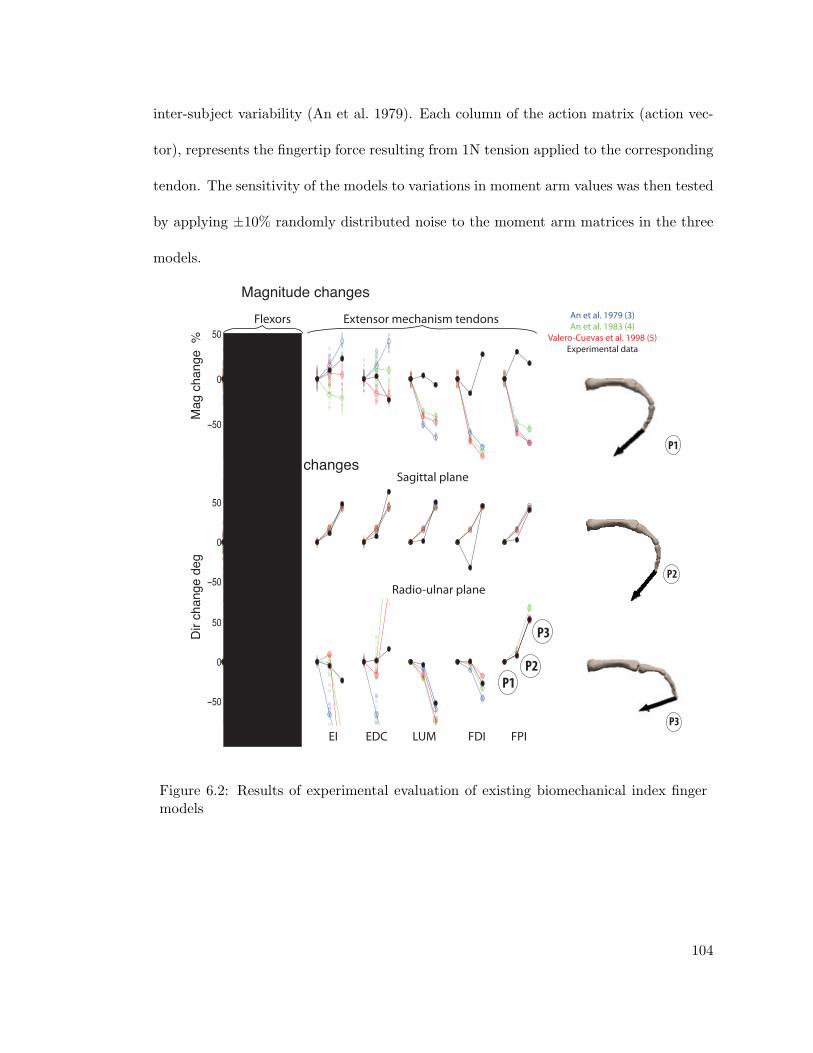
inter-subject variability (An et al. 1979). Each column of the action matrix (action vec-

tor), represents the fingertip force resulting from 1N tension applied to the corresponding

tendon. The sensitivity of the models to variations in moment arm values was then tested

by applying ±10% randomly distributed noise to the moment arm matrices in the three

models.

An et al. 1979 (3)An et al. 1983 (4)

Valero-Cuevas et al. 1998 (5)Experimental data

1 2

Magnitude changes

Direction changes

FDP FDS EI EDC LUM FDI FPI

Flexors Extensor mechanism tendons

Sagittal plane

Radio-ulnar plane

Mag

cha

nge

%D

ir ch

ange

deg

−50

0

50

−50

0

50

−50

0

50

P1P2

P3

P1

P2

P3

Figure 6.2: Results of experimental evaluation of existing biomechanical index fingermodels

104

6.3 Results

Fig. 6.2 shows the changes in magnitude and direction of each tendons action vector

relative to the first posture for all models (and data). The changes in magnitude observed

in all three models disagree with one another and with those observed in experimental

data. The changes in direction for tendons other than EI and EDC (sagittal plane) and

LUM, FDI and FPI (radio-ulnar plane) also do not match with corresponding changes

in experimental data. The components of the action vector for the EDC and EI in

the radio-ulnar plane are very small and hence corresponding directional errors can be

neglected.

Fig 6.3 shows the absolute magnitude and direction errors for the An-Chao normative

model (An et al. 1979), which is the only one of the three models here that explicitly

represents the extensor mechanism. The figure shows the errors for each tendon’s action

vector when evaluated against the experimental data in the three finger postures. The

absolute errors in magnitude are very large. The direction errors for some of the intrinsic

tendons is smaller compared to the errors for the EDC and EIP. This is a little counterin-

tuitive considering that these are relatively ‘simple tendons’. Also the errors are different

in different postures as can be expected since the tension distribution in the extensor

mechanism is known to change with posture.

The flexors with larger moment arms are more sensitive to variations as compared to

the extensors and the intrinsics. A ±10% change in moment arm values in these tendons

results in 30-40 degree change in fingertip force direction and around 50% change in

magnitude.

105

Magnitude errors

Direction errors

FDP FDS EIP EDC LUM FDI FPI0

20

40

60

Dir

erro

r (de

gree

s)

FDP FDS EIP EDC LUM FDI FPI0

200

400

600

800

1000

Mag

erro

r %

Fully �exedTapFully extended

Figure 6.3: Absolute magnitude and direction errors for the An-Chao Normative modelwhen tested with experimental data from a cadaveric index finger

106

The three models of the index finger disagree with one another and with the experi-

mental data. They are sensitive to perturbations and result in large variations in fingertip

force output. Hence it is important to develop subject-specific models of these complex

systems that have been informed by experimental data.

6.4 Discussion

Our experimental validation of the existing models of the index finger revealed that

existing models have large magnitude and directional errors. More detailed and accurate

representations of the topology and parameters of the extensor mechanism, inferred from

experimental data, are necessary to develop reliable biomechanical models of the finger

to understand motor control of manipulation and changes upon damage.

Acknowledgment

Coauthors Dr. Hod Lipson and Dr. Francisco Valero-Cuevas. The hand surgeons, Dr.

Vincent Hentz, Dr. Caroline Leclercq, Dr. Isabella Fassola and Dr. Nina Lightdale for

doing the cadaveric dissections. Dr. Jae Woong Yi for building the cadaver actuation

setup. NSF Grants EFRI-COPN 0836042 and NIH Grants AR050520 and AR052345 to

FVC.

107

Chapter 7

Study of the Sensitivity of Fingertip Force Output to

Topology and Parameters of the Extensor Mechanism

Using a Novel Finite Element Analysis Simulator

7.1 Abstract

How the extensor mechanism of the fingers distributes forces from multiple muscles to

multiple joints resulting in fingertip force is not clearly understood. Existing muscu-

loskeletal modeling software cannot model interactions of complex tendon networks with

bones. Here we present a novel simulator based on the finite element method that models

the mechanics of interactions of any elastic network of strings with arbitrarily shaped

solids like bones. We validated this simulator using experimental data from the actuation

of a latex rubber network draped on a solid hemispherical dome and observed that the

model matches the experimental data closely with an overall RMS error of 11.5% in forces.

We then simulated the extensor mechanism of the index finger as an elastic tendon net-

work of strings draped over an MRI scan of the finger bones. Since the properties of the

108

extensor mechanism and its influence on fingertip force are poorly understood, we per-

formed a sensitivity analysis where we varied the positions of connectivity of the network,

the cross sectional area of the different bands, the resting lengths of these components

and the topology (or connectivity) of the network itself. We simulated these changes in

three different finger postures. We observed that the fingertip force output is sensitive

to the posture, the positions of the nodes, the resting lengths of the components and the

topology of the extensor mechanism and less sensitive to the cross sectional areas of the

different bands.

7.2 Introduction

Forces generated by the muscles actuating the fingers are transmitted to the joints through

a complex network of tendons called the extensor mechanism. The role of the extensor

mechanism in human manipulation is not clearly understood (Valero-Cuevas 2000a, Lee,

Chen, Towles & Kamper 2008, Landsmeer 1949, Haines 1951, Littler 1967, Harris Jr &

Rutledge Jr 1972). Studies have shown that the extensor mechanism transmits forces dif-

ferently at different finger postures. It has also been shown that the different components

of the extensor mechanism have different elastic properties (Garcia-Elias, An, Berglund,

Linscheid, Cooney & Chao 1991). While most studies of the extensor mechanism use

the Winslow’s rhombus representation, other representations have also been suggested in

the literature (Garcia-Elias, An, Berglund, Linscheid, Cooney Iii & Chao 1991). How

fingertip force output changes with these parameters: locations of the network nodes, the

109

elastic properties of the network or the topological representation (the network connec-

tivity) itself, has not been studied.

Computational modeling can be a useful tool to understand the mechanical behavior

of the extensor mechanism and its sensitivity to the properties mentioned above. Most ex-

isting computational models of the fingers do not represent the interactions of the various

components of the extensor mechanism. They either consist of combinations of Landsmeer

models for tendon routing (Sancho-Bru et al. 2001) or are represented as constant moment

arm matrices (An et al. 1983, Spoor 1983, Leijnse et al. 1992, Leijnse 1996, Valero-Cuevas

et al. 1998). The An-Chao model (Chao & An 1978a, An et al. 1979), one of the earli-

est developed mathematical representations of the finger, which has been used in several

studies in the literature (Li et al. 2001, Harding et al. 1993, Dennerlein, Diao, Mote Jr

& Rempel 1998, Weightman & Amis 1982), explicitly modeled the distribution of forces

within the extensor mechanism. But it assumed a fixed distribution of tendon tensions

among the different bands of the extensor mechanism for all postures. However, ear-

lier studies had shown that the geometry of the bands as well as the force distribution

through them, change significantly with posture (Garcia-Elias, An, Berglund, Linscheid,

Cooney Iii & Chao 1991, Sarrafian et al. 1970, Micks & Reswick 1981). Recently, a dy-

namic simulator of the hand has been developed (Sueda et al. 2008) that simulates the

interactions of these tendon network interactions. But it is aimed at producing realistic

hand motion for graphics applications and the force transmission capability of this model

has not been validated with experimental data.

Most existing musculoskeletal modeling software like SIMM (Motion Analysis Corpo-

ration) (Delp & Loan 1995), AnyBody (AnyBody Technology) (Damsgaard et al. 2006)

110

or MSMS (Davoodi et al. 2007) do not have the capability to model tendinous networks.

They are based on single line of action models for the musculotendons or use of wrapping

surfaces and via points to model the routing of musculotendons around joints. See chap-

ter 2 for more details about these models. These techniques do not suffice to model the

wrapping of a network of tendons on solid bony surfaces. Hence, we developed a novel

finite element method based simulator that models the mechanical force transmission by

an elastic network of tendons draped on any arbitrary solid (like bones) which we present

here. It is an advancement of the relaxation algorithm based simulator presented earlier

(Lipson 2006, Valero-Cuevas & Lipson 2004). It can be effectively used to model isometric

force production in complex biomechanical systems. We validate this solver by actuating

a latex network draped on a hemispherical dome. We then use this simulator to model

the finger extensor mechanism to study the sensitivity of fingertip output to variation in

the parameters and topology of the extensor mechanism.

7.3 Methods

7.3.1 The Tendon Network Simulator

Previously, a relaxation algorithm was used to simulate mechanics of tendon networks in

2D and for networks on simplified models of bones in 3D(Valero-Cuevas & Lipson 2004).

Here we use the finite element method to expand this work to develop a simulator of

elastic networks interacting with arbitrarily shaped rigid objects. The solver assumes the

solid surface to be fixed and frictionless, and the elastic network is free to deform and

slide over the surface while the resulting contact forces can be determined.

111

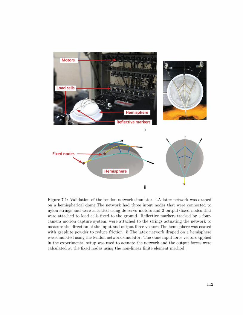
Motors

Load cells

Hemisphere

Re�ective markers

Fixed nodes

Hemisphere

i

ii

Figure 7.1: Validation of the tendon network simulator. i.A latex network was drapedon a hemispherical dome.The network had three input nodes that were connected tonylon strings and were actuated using dc servo motors and 2 output/fixed nodes thatwere attached to load cells fixed to the ground. Reflective markers tracked by a four-camera motion capture system, were attached to the strings actuating the network tomeasure the direction of the input and output force vectors.The hemisphere was coatedwith graphite powder to reduce friction. ii.The latex network draped on a hemispherewas simulated using the tendon network simulator. The same input force vectors appliedin the experimental setup was used to actuate the network and the output forces werecalculated at the fixed nodes using the non-linear finite element method.

112

We model the elastic tendon networks using cable elements that transmit forces in

tension but not in compression, that are connected at nodes that only have displacement

degrees of freedom (three, similar to a 3D truss). The solid surface on which this network

is draped is modeled as a rigid tessellated solid. The boundary conditions include the

input force vectors applied on the network (by muscles in the body) in 3D and zero

displacements at the nodes where the elastic network attaches to the solid (the tendon

slips). We used the incremental-iterative Newton-Raphson (NR) technique to solve the

non linear finite element problem (Crisfield 1991). First the initial configuration of the

network was defined in the same 3D coordinate space as the rigid polygon model of the

bones. Then in every large iteration of the process, we performed i. a node penetration

test – If a node was inside the tessellated solid, we pushed it to the surface and held it

there by a constraint spring and ii. an element penetration test –We tested multiple points

along the length of the element and created new nodes at points penetrating the solid and

pushed them to the surface. Once node and element-penetration tests were performed,

the tangent stiffness matrix and residue vector were calculated for every element. These

were assembled and the displacements of the nodes were calculated for small increments

in load using the iterative Newton-Raphson method. The node- and element-penetration

tests were repeated for every load increment. Please see the appendix for more details.

7.3.2 Experimental Validation of the Tendon Network Simulator

We draped a network made of latex rubber on a plastic surface which formed a part of

a hemisphere. The network had three input nodes and two output nodes (Fig. 7.1).

We connected the input nodes using nylon strings to dc servo motors. The strings were

113

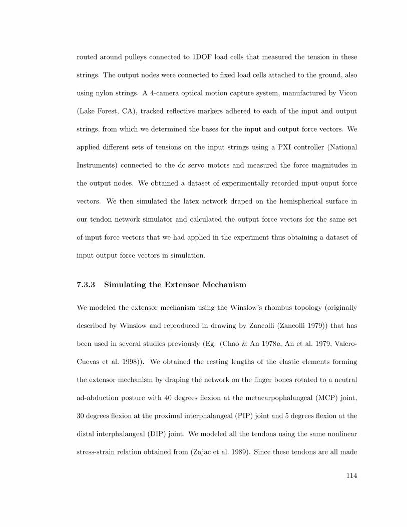
routed around pulleys connected to 1DOF load cells that measured the tension in these

strings. The output nodes were connected to fixed load cells attached to the ground, also

using nylon strings. A 4-camera optical motion capture system, manufactured by Vicon

(Lake Forest, CA), tracked reflective markers adhered to each of the input and output

strings, from which we determined the bases for the input and output force vectors. We

applied different sets of tensions on the input strings using a PXI controller (National

Instruments) connected to the dc servo motors and measured the force magnitudes in

the output nodes. We obtained a dataset of experimentally recorded input-ouput force

vectors. We then simulated the latex network draped on the hemispherical surface in

our tendon network simulator and calculated the output force vectors for the same set

of input force vectors that we had applied in the experiment thus obtaining a dataset of

input-output force vectors in simulation.

7.3.3 Simulating the Extensor Mechanism

We modeled the extensor mechanism using the Winslow’s rhombus topology (originally

described by Winslow and reproduced in drawing by Zancolli (Zancolli 1979)) that has

been used in several studies previously (Eg. (Chao & An 1978a, An et al. 1979, Valero-

Cuevas et al. 1998)). We obtained the resting lengths of the elastic elements forming

the extensor mechanism by draping the network on the finger bones rotated to a neutral

ad-abduction posture with 40 degrees flexion at the metacarpophalangeal (MCP) joint,

30 degrees flexion at the proximal interphalangeal (PIP) joint and 5 degrees flexion at the

distal interphalangeal (DIP) joint. We modeled all the tendons using the same nonlinear

stress-strain relation obtained from (Zajac et al. 1989). Since these tendons are all made

114

of collagenous fibers, this is a valid assumption. We calculated the element cross-sectional

areas for each of the bands of the extensor mechanism using values for the force length re-

lationship provided in (Garcia-Elias, An, Berglund, Linscheid, Cooney & Chao 1991). We

obtained the polygonal surface model of scanned hand bones from the Stereolithography

Archive at Clemson University. We studied the finger in three postures, all in neutral ad-

abduction : i. Fully flexed (50 60 20) ii. Tap (40 30 5) and iii. Fully extended (20 20 10).

(Note that the values in the parentheses represent the flexion joint angles, in degrees, at

the MCP, PIP and DIP, respectively for each of the postures.) There were three inputs to

the model representing forces from four of the muscles actuating the index finger- the first

palmar interosseous (FPI), extensor indicis (EI), extensor digitorum communis (EDC)

and the first lumbrical (LUM). The EI and the EDC which have a very similar line of

action (An et al. 1983) were modeled as one input. The extensor mechanism attached to

the finger bones at two points, the central and the terminal slips on the middle phalanx

and distal phalanx respectively (Fig. 7.2(a)). We did not model the retinacular and the

oblique retinacular ligaments (Bendz 1985). Solving the non linear finite element problem

gave us the displacements of all the nodes of the network and the reaction forces at the

two slips. We obtained joint torques from tendon tensions and calculated fingertip force

output using the formulation F = J−Tτ (Valero-Cuevas 2009) where F is the fingertip

force output, J is the jacobian transforming joint angle velocities to fingertip velocities

and τ is the vector of joint torques (Fig. 7.2(a)).

115

7.3.4 Sensitivity Analysis

Sensitivity analysis is a common procedure in computational modeling to see the effect

of changes in parameter values or inputs on the output of the model. Local sensitivity

analysis is one of the simplest forms where the parameters/inputs to the model are varied

one at a time keeping the others fixed at the base value (Scovil & Ronsky 2006, Raphael,

Tsianos & Loeb 2010). We tested the local sensitivity of the fingertip force output to

four different properties of the extensor mechanism : i. Node positions of eight nodes

forming the extensor mechanism, ii. Cross-sectional areas of 10 elements, iii. Resting

lengths of 10 elements iv. Topology of the network (Fig. 7.2(b)). We assumed palmar-

dorsal symmetry for all properties (so number of parameters were reduced to half their

total number). We varied each property individually and measured changes in fingertip

force magnitude and direction in reference to those generated using the base network

with nominal values for the properties (defined in the previous section). For the first

three properties, we generated 100 samples each, consisting of random combinations of

parameter values lying between ±25% of the range of possible values for the parameter

of interest (i.e. 100 combinations of node positions, 100 combinations of cross sectional

areas, etc.) To understand the effect of topology, 16 discrete topologies were studied,

formed by different combinations of inclusion and removal of four bands of the extensor

mechanism (Fig. 7.2(b)).

116

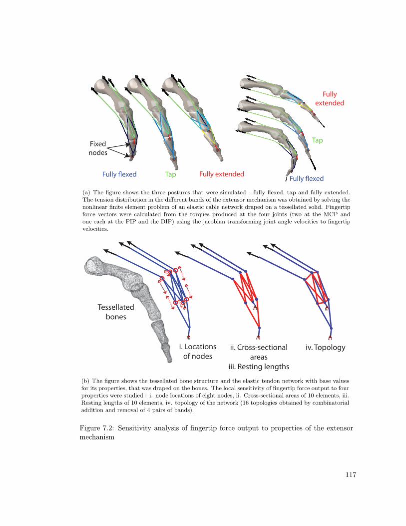
Fully �exed

Tap

Fully extended

Fully �exed Tap Fully extended

Fixed nodes

(a) The figure shows the three postures that were simulated : fully flexed, tap and fully extended.The tension distribution in the different bands of the extensor mechanism was obtained by solving thenonlinear finite element problem of an elastic cable network draped on a tessellated solid. Fingertipforce vectors were calculated from the torques produced at the four joints (two at the MCP andone each at the PIP and the DIP) using the jacobian transforming joint angle velocities to fingertipvelocities.

Tessellated bones

i. Locations of nodes

ii. Cross-sectional areas

iii. Resting lengths

iv. Topology

(b) The figure shows the tessellated bone structure and the elastic tendon network with base valuesfor its properties, that was draped on the bones. The local sensitivity of fingertip force output to fourproperties were studied : i. node locations of eight nodes, ii. Cross-sectional areas of 10 elements, iii.Resting lengths of 10 elements, iv. topology of the network (16 topologies obtained by combinatorialaddition and removal of 4 pairs of bands).

Figure 7.2: Sensitivity analysis of fingertip force output to properties of the extensormechanism

117

7.4 Results

7.4.1 Results of validation of the tendon network

The reaction forces determined using the tendon network simulator matched the ex-

perimental data closely with a normalized RMS error of 11.5%. Figure 7.3 shows the

validation results. To ensure that any arbitrary network would not produce the same

reaction forces, we also simulated a latex network slightly altered from the one used for

the experiments in our tendon network simulator. We then compared the reaction forces

predicted for the altered network with the previous experimentally measured values. The

errors in this case were much larger.

7.4.2 Results of Sensitivity Analysis

We observed that the sensitivity of the fingertip force output to the different properties of

the extensor mechanism varied largely with finger posture (Fig. 7.4). This was not very

surprising because it has been shown in early cadaver studies that the tension distribution

within the bands of the extensor mechanism changes with finger posture (Sarrafian et al.

1970, Micks & Reswick 1981) with more force being transmitted to the terminal slip

in extended postures and to the central slip in flexed postures. The sensitivity of the

fingertip force is also different for the different properties of the extensor mechanism.

Based on the local sensitivity analysis performed here, we observe that the fingertip

output is most sensitive to the resting lengths of the bands of the extensor mechanism.

±25% perturbation of the resting length can lead to more than 40 degrees of change

in fingertip output and more than 200% change in force magnitude. Topology of the

118

0 1 2 3 4 50

1

2

3

4

5

RF Magnitude (Model) in N

RF

Mag

nitu

de (D

ata)

in N

0 1 2 3 4 50

1

2

3

4

5

RF Magnitude (Model) in N

RF

Mag

nitu

de (D

ata)

in N

RF Node 1RF Node 2x=y line

Node 1

Node 2

Node 1

Node 2

Figure 7.3: Comparison of experimental and simulated data for latex network drapedon hemisphere. The figure shows a comparison of force magnitudes at the two fixednodes of the latex network recorded experimentally vs. calculated in simulation usingthe tendon network simulator. The left column shows results when the same networktopology and parameters were generated in simulation as those used for the experiment.The force magnitudes in the experimental and simulated cases matched closely seen bytheir proximity to the x=y line. The right column shows comparison of the sameexperimental data with simulated data from a network with a modified topology thanthe one used for the experiment. The experimental and simulated force magnitudesdo not align closely to the x-y line unlike before. This demonstrated that the tendonnetwork simulator accurately represented the physical latex network and the matchingup of the experimental and simulated data was not mere coincidence.

119

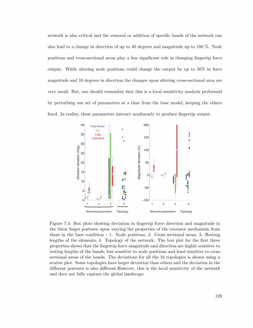
network is also critical and the removal or addition of specific bands of the network can

also lead to a change in direction of up to 40 degrees and magnitude up to 180 %. Node

positions and cross-sectional areas play a less significant role in changing fingertip force

output. While altering node positions could change the output by up to 50% in force

magnitude and 10 degrees in direction the changes upon altering cross-sectional area are

very small. But, one should remember that this is a local sensitivity analysis performed

by perturbing one set of parameters at a time from the base model, keeping the others

fixed. In reality, these parameters interact nonlinearly to produce fingertip output.

0

5

10

15

20

25

30

35

40

Dire

ctio

n de

viat

ion

(deg

)

−100

−50

0

50

100

150

200

Mag

nitu

de d

evia

tion

(%)

1 2 3 4 1 2 3 4

Network parameters Topology Network parameters Topology

Fully �exedTapFully

extended

Figure 7.4: Box plots showing deviation in fingertip force direction and magnitude inthe three finger postures upon varying the properties of the extensor mechanism fromthose in the base condition : 1. Node positions, 2. Cross sectional areas, 3. Restinglengths of the elements, 4. Topology of the network. The box plot for the first threeproperties shows that the fingertip force magnitude and direction are highly sensitive toresting lengths of the bands, less sensitive to node positions and least sensitive to crosssectional areas of the bands. The deviations for all the 16 topologies is shown using ascatter plot. Some topologies have larger deviation than others and the deviation in thedifferent postures is also different.However, this is the local sensitivity of the networkand does not fully capture the global landscape.

120

7.5 Discussion

Here we have presented a novel simulator to model the interactions of elastic tendon

networks with arbitrarily shaped bones in three-dimensions. We have validated this sim-

ulator with experimental data from a latex network draped on a hemispherical dome

and shown that the model prediction match closely with the data (RMS error of 13% in

reaction forces). Some reasons for the slight mismatch between the model and the ex-

perimental data could be attributed to measurement errors, friction on the hemisphere,

errors in calculation of force vector direction from motion capture data and also replica-

tion of the exact experimental setup in simulation (Eg. location of the network on the

hemisphere, location of the fixed nodes where the reaction forces were measured, etc).

It has also been shown in cadaveric observational studies of the extensor mechanism

(Garcia-Elias, An, Berglund, Linscheid, Cooney Iii & Chao 1991) that there are large

changes in spatial arrangement of the components of the extensor mechanism in the

different postures.We observed this in simulation too. While the actual deformation of

the components itself was not very large, the components did shift and the distribution

of tension in them changed substantially with finger posture. This was also seen in

the sensitivity analysis where the sensitivity of the fingertip force output direction and

magnitude was different in different postures.

We model the extensor mechanism as a set of elastic strings connected to each other

at distinct nodes. This is an approximation of the true structure which consists of several

thin elastic collagenous fibers interlaced to form a sheet of collagen. Also the base network

assumed here is based on the Winslow’s rhombus topology and the node positions were

121

chosen to approximately represent the network as seen in textbooks of anatomy, based

on anatomical observation in cadaveric specimens. In Chapter 8 we will infer a more

accurate topology and set of parameter values directly from experimental data collected

by testing of a cadaveric index finger.

As mentioned earlier, the sensitivity analysis described here is a local sensitivity analy-

sis where individual properties were varied independently keeping all the other properties

fixed at the base level. But since these different properties interact in a nonlinear fash-

ion, the sensitivity profile could change if different base parameter values are assumed

for the properties or if multiple properties are varied simultaneously. A more rigorous

sensitivity analysis based on Monte Carlo sampling methods (Santos, Bustamante &

Valero-Cuevas 2009) would be more comprehensive.

The sensitivity analysis demonstrated that the fingertip force output is most sensitive

to topology and resting lengths of the bands. For a stiff elastic network like the tendon

networks, the deformation of the network upon loading with low forces like the ones

applied here or those applied by muscles in the human fingers is very small. Hence, the

largest effect of fingertip force is due to changes in connectivity of the network because

force distribution largely depends on which bands are transmitting forces. Changing

the resting length or changing the topology perform the same function of changing this

connectivity. Hence the fingertip force output is most sensitive to these properties.

While the tendon network simulator here has been used to determine finger forces in

an isometric scenario, it could be easily extended to simulate slow finger movements as a

quasi-static solver. Joint torques would be calculated the exact same manner as shown

122

here and the joint angles of the finger are changed to reach a new equilibrium posture of

the finger.

7.6 Appendix

The tendon network simulator relies on solving a nonlinear finite element problem. The

tendon network is represented as a set of elastic elements connected to one another at

distinct nodes. These elements have the same elastic properties as human tendons and

they exert forces only in tension. Hence the network is represented as a truss network but

with elements transmitting force only in tension (string or cable network). The bones

are represented as tessellated solids, rotated to represent the posture being simulated.

They are modeled as rigid solids and their elastic deformations are neglected. The elastic

network drapes on this solid and the algorithm ensures the network does not penetrate

this solid. The flow chart of the algorithm used to solve the finite element problem is

shown in Fig. 7.5. It is based on an incremental-iterative Newton-Raphson method

(Crisfield 1991).

The external force vector totF consisting of x,y,z components of the external force

vectors acting on each of the nodes of the tendon network is applied to the system in

parts (j)F.

(j)F =(j−1)F +(tot)FN

123

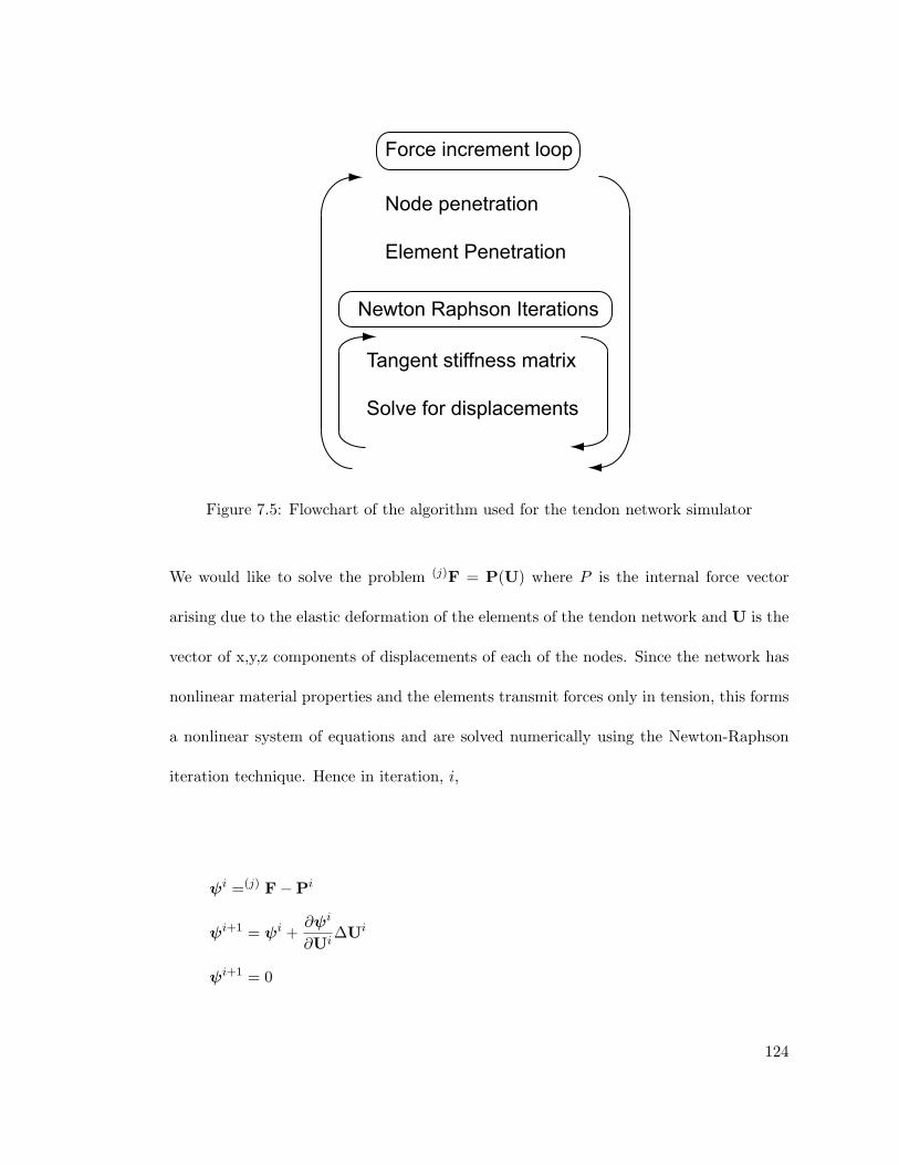
Node penetration

Element Penetration

Force increment loop

Newton Raphson Iterations

Tangent stiffness matrix

Solve for displacements

Figure 7.5: Flowchart of the algorithm used for the tendon network simulator

We would like to solve the problem (j)F = P(U) where P is the internal force vector

arising due to the elastic deformation of the elements of the tendon network and U is the

vector of x,y,z components of displacements of each of the nodes. Since the network has

nonlinear material properties and the elements transmit forces only in tension, this forms

a nonlinear system of equations and are solved numerically using the Newton-Raphson

iteration technique. Hence in iteration, i,

ψi =(j) F−Pi

ψi+1 = ψi +∂ψi

∂Ui∆Ui

ψi+1 = 0

124

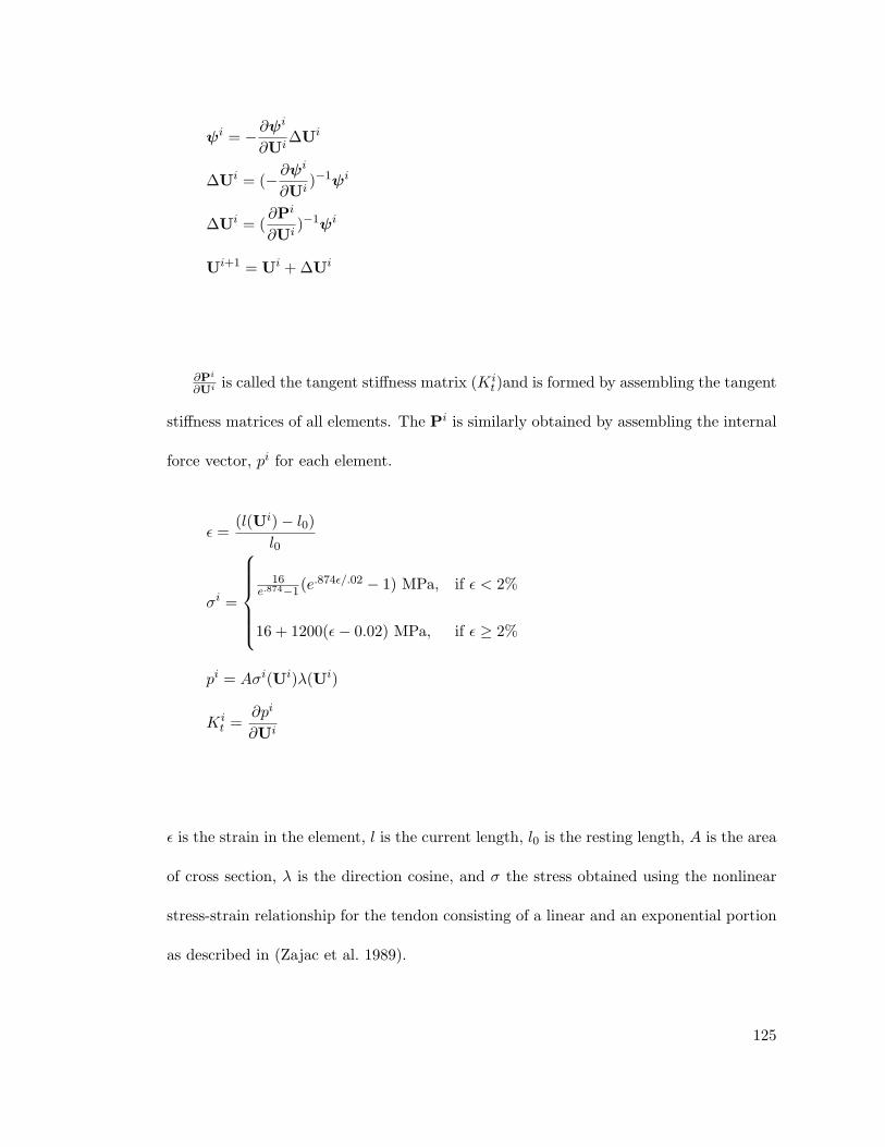
ψi = −∂ψi

∂Ui∆Ui

∆Ui = (−∂ψi

∂Ui)−1ψi

∆Ui = (∂Pi

∂Ui)−1ψi

Ui+1 = Ui + ∆Ui

∂Pi

∂Ui is called the tangent stiffness matrix (Kit)and is formed by assembling the tangent

stiffness matrices of all elements. The Pi is similarly obtained by assembling the internal

force vector, pi for each element.

ε =(l(Ui)− l0)

l0

σi =

16

e.874−1(e.874ε/.02 − 1) MPa, if ε < 2%

16 + 1200(ε− 0.02) MPa, if ε ≥ 2%

pi = Aσi(Ui)λ(Ui)

Kit =

∂pi

∂Ui

ε is the strain in the element, l is the current length, l0 is the resting length, A is the area

of cross section, λ is the direction cosine, and σ the stress obtained using the nonlinear

stress-strain relationship for the tendon consisting of a linear and an exponential portion

as described in (Zajac et al. 1989).

125

7.6.1 Node and Element Penetration Tests

A node-penetration test was performed to check if any node was penetrating the solid.

This was done by checking the sign of the dot product of the vector from the node to

the centroid of the closest triangle and the outward normal vector to that triangle. If a

node was penetrating the solid, the node was pushed out to the surface by a restoration

force created by a constraint spring element from the nearest point on the surface to the

penetrating node. This spring element had a negligible resting length and high stiffness,

and represented the force that a solid surface applies to prevent penetration. Then an

element-penetration test was performed by repeating the node penetration test at distinct

points on the element. If a point on the element was penetrating the solid, a new node

was created at that point and pushed to the surface in the manner described above.

Acknowledgment

Coauthors Dr. Hod Lipson and Dr. Francisco Valero-Cuevas. Dr. Anupam Saxena

and Qian-Yi Zhou for their inputs. This material is based upon work supported by

the National Science Foundation under Grants No. 0237258 (CAREER award) and No.

0312271 (ITR project); This publication was made possible by Grants Number AR050520

and AR052345 from the National Institutes of Health (NIH). Its contents are solely the

responsibility of the authors and do not necessarily represent the official views of the

National Institute of Arthritis and Musculoskeletal and Skin Diseases (NIAMS), or the

NIH.

126

Chapter 8

Inference of the Topology and Parameters of the Tendon

Networks of the Human Fingers via Sparse

Experimentation

8.1 Abstract

Computational models of biomechanical systems are generally developed using exper-

imentally measured values for specific parameters of the system and fitting this to a

structure that is based on anatomical observations with simplifying assumptions. How-

ever, it is not always feasible to measure all parameters in a system and there is no

guarantee that the assumed anatomical structure of the model is functionally accurate.

As we have demonstrated in chapters 3 and 4, models whose structure and parameter val-

ues are inferred directly from experimental data can be more accurate representations of

the system whether the goal is to obtain subject-specific models or models that generalize

across specimens. However, obtaining a large amount of data from biological systems can

be very expensive. Here we implement a novel method to simultaneously infer the param-

eter values and topology/structure of a three dimensional anatomy-based model of the

127

extensor mechanism of the index finger directly from functional input-output cadaveric

experimental data through intelligent testing that enables the inference with minimal

data points. We show that the models of the extensor mechanism inferred using this

technique more accurately predict fingertip force magnitude and direction in comparison

to a model widely used in the literature.

8.2 Introduction

Understanding neural control of motion and force requires accurate representations of the

‘plant’ or the peripheral musculoskeletal system being controlled. Computational models

of these musculoskeletal systems have been widely used in the literature to understand

how they produce movement and force when actuated by the nervous system(Valero-

Cuevas et al. 2009). These computational models are generally based on anatomical

observations in cadaveric specimens. In most cases, a fixed structure and connectivity

of the musculotendons to the bones and joints is assumed and the model parameters

are obtained using rigorous experimental measurements (Holzbaur, Murray & Delp 2005,

Brown & Loeb 2000, Murray et al. 1995) or calculated based on equilibrium conditions

or solving an optimization problem (Chao & An 1978b, Lee & Rim 1990).

In some cases, it is very difficult to measure certain properties or parameter values of

these musculoskeletal systems experimentally. In many cases musculoskeletal models are

not one-to-one representations of the biological system. They consist of computational

simplifications and hence some parameters of the model may not correspond directly to

a specific properties in the system. For example, muscles with a large insertion are often

128

represented using multiple segments (Holzbaur et al. 2005). Hence an alternative method

of inference of model parameters directly from experimental data has been used in recent

years (Yeo, Tresch & Pai 2008, Gatti & Hughes 2009, Yeo, Mullens, Sandercock, Pai &

Tresch 2011, Raphael et al. 2010). In these studies, model parameters are optimized such

that the difference between the experimental data and the model outputs is minimum.

But then, these studies still make an assumption on the structure of the model : the

topology or the connectivity of the different components, based on the knowledge of the

anatomy. But if this assumed structure itself is not correct, inferring model parame-

ter values from experimental data and fitting them to the wrong structure would not

solve the problem. Hence a new computational method was developed by Valero-Cuevas

et al. (Valero-Cuevas, Anand, Saxena & Lipson 2007) to simultaneously infer model

topology and parameter values of complex biomechanical systems from experimental

data. Moreover this method based on the estimation exploration algorithm developed

by Bongard and Lipson (Bongard & Lipson 2004a, Bongard & Lipson 2005b, Bongard &

Lipson 2005a), demonstrates this inference through minimal experimental data points.

In this method, the concept of predator-prey coevolution is used to optimize a set

of models explaining the data and a set of tests that give most information about the

models. The estimation phase involves optimization of a set of models that best fit the

available experimental data points. This is followed by the exploration phase that involves

finding a test/tests that create most disagreement among the best models obtained so

far. Only these tests are then meant to be carried out on the physical system to obtain

new experimental data points. This process continues till convergence. Hence, instead

of randomly picking experimental tests to perform on the system, only ‘intelligent’ tests

129

chosen by this method are used. Please see (Bongard & Lipson 2005a) for more details on

the method and (Valero-Cuevas, Anand, Saxena & Lipson 2007) for the implementation

in inference of tendon networks. It was shown here (Valero-Cuevas, Anand, Saxena &

Lipson 2007) that this method of inference of structures via ‘intelligent testing’ performed

better than using random tests in speed of convergence to good solutions as well as the

accuracy of the solutions obtained. Here we apply this methodology to simultaneously

infer the topology and parameter values of computational models of the finger’s exten-

sor mechanism from experimental data obtained by actuating a human cadaveric finger.

Please see Chapter 7 for an overview of existing models of the index finger. We compared

the inferred model of the extensor mechanism with the model proposed by Chao and

An (Chao & An 1978a, An et al. 1979) most commonly adopted in the literature and

which is one of the few models that actually explicitly incorporates the interactions of

the components of the extensor mechanism in fingertip force prediction. But this model

assumes constant force distribution through the different bands and no changes with

posture which has been demonstrated in cadaveric studies to not be the case in reality

(Sarrafian et al. 1970, Micks & Reswick 1981).

8.3 Methods

8.3.1 Experimental Data from a Cadaveric Index Finger

The cadaveric experimental setup used to actuate the seven tendons (FDP,FDS,EIP,LUM,FDI,FPI)

of the index finger is described in Chapter 6. Using force control mode (see section 5.3),

we applied a base tension of 1N on the FDP, FDS and the FDI. We applied a set of

130

6 DOF loadcell

Load cells measur-ing tendon tensions

Strings connecting tendons to motors

Fingertip force vector

Figure 8.1: The experimental setup used to record fingertip forces from a freshly frozencadaveric hand. We applied 24 combinations of random inputs lying in the range of 1 to11N to the EIP, EDC, LUM and FPI tendons of the index finger and a base tension of1N on the other three tendons (FDP, FDS and FDI). We recorded the output fingertipforces for each combination of inputs. We repeated this in three different finger postures: fully flexed, tap and fully extended.

131

randomly generated tendon tensions (uniform distribution) lying between 1N and 11N

on the EIP, EDC, LUM and FPI. Whether the FDI attaches to the extensor mechanism

or not has been debated in the literature and there have been contradicting observations

(Salsbury 1937, Garcia-Elias, An, Berglund, Linscheid, Cooney Iii & Chao 1991). We

chose to actuate the FDI with base tension and not consider it as an input to the exten-

sor mechanism. The fingertip was rigidly attached to a 6 DOF load cell (JR3, Woodland,

CA) from which we obtained the fingertip force vector. We repeated this procedure in

three different finger postures : fully flexed, tap and fully extended all in neutral ad-

abduction and flexion-extension joint angles at the MCP, PIP and DIP of (26 62 35), (25

40 30), (5 30 20) degrees, respectively in the three postures. Hence the entire dataset

consisted of 72 tests (24 in each of the three postures).

8.3.2 Modeling Environment

The tendon network simulator used to model the interactions of the elastic tendon net-

works draped on the bones of the index finger is described in detail in Chapter 7. Fig.

8.2 shows the base model along with the properties of the extensor mechanism that were

inferred from the experimental data : i. node positions of 6 nodes (4 variables) forming

the extensor mechanism, ii. resting lengths of 13 elements (7 variables) and iii. topology

of the network : 8 elements (4 variables). We chose to infer these specific properties

based on the sensitivity analysis results in Chapter 7. The node positions were moved

along the length of the outer segment. The resting lengths at any set of node positions

were determined by first draping the network with no input tendon tension in a spe-

cific posture (neutral ad-abduction, 40,30,5 degrees flexion at the MCP, PIP and DIP,

132

respectively) and then altering this length by the factor determined by the optimization

variable corresponding to this parameter. The topology was varied by either including

or removing the specific eight bands of the extensor mechanism shown in Fig. 8.1. We

assumed symmetry of the network topology and parameters about the sagittal plane of

the finger for computational simplicity. The extensor mechanism model was assumed to

have three inputs: the LUM, the FPI and one extensor input. The EIP and the EDC were

combined as one single tendon and the tension magnitudes applied to these two tendons

were summed together. Given, a set of topology-parameter values, input force magni-

tudes and finger posture, the fingertip force vector was determined solving the nonlinear

finite element problem, calculating joint torques and using the Jacobian matrix mapping

the joint angle velocities to end point velocities as described in Chapter 7.

Tessellated bones

i. Locations of 6 nodes

(4 variables)

ii. Resting lengths of 13 elements(7 variables)

iii. Topology : 8 elements

(4 variables)

Figure 8.2: The tendon network simulator and the variables being inferred. The tendonnetwork was modeled as a network of elastic cable elements draped on a tessellatedmodel of the bones. Three properties of the network were varied :i. Node positions of6 nodes (4 variables), ii. Resting lengths of 13 elements (7 variables) and iii. Topologyof the network : 8 elements (4 variables).

133

Test suite

Converged?

5N 5N3N

1N1.5N3N

Start3 Random testsMeasured data

Evolve models

No

End

Two best tests selected

Estimation Exploration

1N3N3N

Identify most `intelligent’

tests (posture +

tendon tensions)

Figure 8.3: The estimation exploration algorithm. The algorithm began with threerandom tests consisting of input tendon tensions and experimentally recorded finger-tip forces in three postures (One test in each posture). These were used to optimizeindividually three models of the network minimizing errors in fingertip force directionand magnitude between the experimental data and model prediction. This is the es-timation phase. This was followed by the exploration phase where the two tests thatcause maximum disagreement in fingertip force magnitude and direction between theoptimized models from the estimation phase were picked. These data points from theexperimental dataset were then added to the test suite and used for the estimation.This coevolution of models and tests was carried out for six iterations.

134

8.3.3 Inference Algorithm

We used the estimation-exploration algorithm to infer the topology and parameter values

of the extensor mechanism (Bongard & Lipson 2004a, Bongard & Lipson 2005b, Bongard

& Lipson 2005a, Valero-Cuevas, Anand, Saxena & Lipson 2007). Our inference began with

a test suite consisting of three random data points measured experimentally, i.e three sets

of input tendon tensions and experimentally recorded fingertip forces in three postures

(1 test in each posture). These were used to optimize individually three models of the

network in parallel in what is called the estimation phase (Fig. 8.3). The optimization

cost function was a weighted sum of the fingertip force magnitude error and fingertip

direction error, which we shall call the fitness error. The fingertip force magnitude error

was the root mean squared (RMS) normalized magnitude error and the force direction

error was the RMS direction angle error of the fingertip force vector over all the tests

in the test suite. We used a Markov-Chain Monte Carlo based optimization algorithm

for the estimation. The estimation phase was followed by the exploration phase. Here

the tests competed amongst themselves (each test consisting of posture and input tendon

tensions) to create largest disagreement among the three optimal models obtained in the

estimation phase. The disagreement produced by a test was measured by the variance

in fingertip force magnitude (or fingertip force direction) when this test was applied

to the three optimal models from the estimation phase, in simulation. Two tests were

selected, one which when applied to the three models in simulation, resulted in the largest

variance in fingertip force magnitude and the other, which resulted in largest variance

in fingertip force direction. The experimental data points corresponding to these two

135

new tests were then added to the test suite and the estimation was repeated. This

co-evolution of models that explained the available data points in the test suite and of

tests that caused most disagreement among the optimal models, was repeated till we

either ran out of experimental data points, the error in the estimation phase stopped

improving or the error was below a certain bound which was defined by the errors in

experimental measurement of joint angles and segment lengths (See below for details).

This entire inference algorithm was run in a parallel computing environment using the

Matlab Parallel Computing toolbox on a computer cluster at the USC High Performance

Computing and Communications Facility.

We implemented the An-Chao normative model (Chao & An 1978a, An et al. 1979) of

the index finger to obtain moment arm values for the tendons of interest (EIP, EDC, LUM

and FPI) in the three finger postures described above. We scaled the model based on the

length of the middle phalynx (An et al. 1979). We obtained fingertip force vector using

the equation (Valero-Cuevas 2009), Ftip = J−TRFm where Ftip is the fingertip wrench

vector, J is the Jacobian matrix mapping joint angle velocities to fingertip velocities, R

is the moment arm matrix, and Fm is the vector of tendon tensions. We only used the

fingertip force components of the fingertip wrench vector for this study (not the torque

produced at the fingertip).

We compared the errors of the inferred models when tested with all the data points

in our dataset (72 tests, 24 in each of the three postures) against the errors for the An-

Chao model (Chao & An 1978a, An et al. 1979). We compared the errors of the fingertip

force direction and magnitude only in the sagittal plane of the finger. The ad-abduction

force component arises from the ad-abduction torque at the MCP which is governed by

136

the location of the input tendons with respect to the joint center and not the properties

(topology and parameters) of the extensor mechanism we were trying to infer. The RMS

magnitude errors (errormag) and RMS direction errors (errordir) were calculated using

the equations below:

errormag =√

(1N

N∑i=1

(‖Fmod‖ − ‖Fexp‖

‖Fexp‖ × 100)2)

errordir =√

(1N

N∑i=1

(cos−1(Fmod

‖Fmod‖ ·Fexp

‖Fexp‖))2)

where errormag and errordir are the errors in fingertip force magnitude and direction,

respectively, N is the total number of tests in the data set (N=72 in our case), Fmod

is the fingertip force magnitude in the model, Fexp is the experimental fingertip force

magnitude.

8.3.4 Experimental Measurement Error

Errors in measurement of joint angles and segment lengths are almost unavoidable in

experiments with biological specimens like the cadaveric index finger (using current mea-

surement techniques: ruler and goniometer/motion capture). This is because of the

existence of non-engineering joints and the presence of skin and fat over the bones whose

length and posture we are trying to measure. These errors in measurement lead to er-

rors in fingertip force direction and magnitude largely because of the nonlinear Jacobian

matrix mapping joint angle velocities to fingertip velocities that also is involved in the

transformation of joint torques to fingertip force. Our inference algorithm will only be

137

able to obtain models that are as accurate as the experimental data; in other words,

the experimental measurement error defines the bound/limit on the fitness error of the

models being inferred. We performed a Monte Carlo analysis by perturbing the joint

angles defining the posture of the finger by ±5 degrees and segment lengths by ±5% and

calculated the fingertip force direction and magnitude errors in simulation, keeping the

network topology and parameters fixed. This determined the experimental uncertainty

bound and any model with errors below this bound would be a valid solution to the

problem.

8.4 Results

The results presented here are based on four separate runs of inference using the estimation-

exploration algorithm. Each inference run consisted of six iterations of the estimation

and exploration phases. A total of thirteen intelligent tests were introduced. Since each

run inferred three independent models, we obtained 12 ‘optimal’ models at the end of four

runs. We compared the RMS errors in force magnitudes and directions of the sagittal

components of the fingertip force vectors predicted using the An-Chao model as well as

the twelve inferred models. We chose to only compare the sagittal components because

the ad-abduction component of the force vector arises largely from the moment arms of

the tendons about the MCP which are not part of the extensor mechanism and hence

not varied in the inference process. Fig. 8.4 shows the comparison results. We only show

the mean and std deviation of the best five models obtained from the inference. The

RMS magnitude errors for the An-Chao model was about five times larger than the mean

138

error for the five best inferred models. The directional errors were also 1.6 to two times

larger than in the An-Chao model compared to the inferred models. The direction errors

for the fully flexed posture were the largest for both types of models followed next by

the tap posture and then the fully extended posture with the lowest errors. The band

of experimental uncertainty shown in the figure was generated by doing a Monte Carlo

analysis where the joint angles were perturbed by ±5 degrees and the segment lengths

by ±5%, keeping the network topology and parameters fixed. These experimental errors

resulted in an error of up to 1.5N in fingertip force magnitude and 14.5 degrees in force

direction. This forms the bound on the accuracy of the inference algorithm. Any model

with errors below this bound is a valid solution to the problem.

The best five inferred models of the extensor mechanism are shown in the fully ex-

tended posture in Fig. 8.5. The color map indicates the tension in each of the bands

of the extensor mechanism. The models differ in their topology and parameter values,

but have a similar fingertip force direction and magnitude error. This demonstrates the

issue of non-uniqueness that has been discussed in earlier work as well (Valero-Cuevas,

Anand, Saxena & Lipson 2007). We discuss more details about unobservability and

non-uniqueness in Chapter 9.

139

Experimental uncertainty

Full flex Tap Full Ext0

1

2

3

4

5

6

RM

S M

ag e

rror (

N)

An Chao 1979Opt

Full flex Tap Full Ext0

5

10

15

20

25

30

35

40

45

RM

S D

ir er

ror d

eg

Figure 8.4: Comparison of magnitude and direction errors of the saggital plane compo-nent of the fingertip force vector in the best five inferred models vs. An-Chao normativemodel (Chao & An 1978a, An et al. 1979) in the three finger postures fully flexed, tapand fully extended. The RMS magnitude errors as well as directional errors were muchlarger for the An-Chao model compared to the inferred models in each of the threepostures.

140

5

10

15

20

25 N

0

Figure 8.5: The best five inferred models obtained using the estimation-explorationalgorithm. These models have similar input-output behavior but vary in their topologyand parameters, demonstrating non-unique solutions.

141

8.5 Discussion

Here we have demonstrated for the first time the inference of a functional 3-dimensional

model of a musculoskeletal system from experimental data collected from an intact cadav-

eric system using intelligent testing. The inferred models capture the functional behavior

of the system more accurately than the model most commonly used in the literature.

The An-Chao model as well as its modified versions (Weightman & Amis 1982) do not

explicitly model the elastic properties of the tendon networks or the physics of interactions

of the different components constituting these networks. Another big drawback of the

An-Chao model is that it assumes a fixed distribution of tendon tensions in the different

components with changes in posture. But cadaveric studies have shown that the geometry

of the bands as well as the force distribution through them, change significantly with

posture (Garcia-Elias, An, Berglund, Linscheid, Cooney Iii & Chao 1991, Sarrafian et al.

1970, Micks & Reswick 1981). The models inferred here give insight on how the geometry

and force distribution changes in the different finger postures.

The inferred models had a fingertip direction error of 10-25 degrees (in the sagittal

plane). While this may seem a like a large error, one should keep in mind that fingertip

force output is very sensitive to measurement in joint angles (Goehler & Murray 2010)

as has been demonstrated using the Monte Carlo analysis. Hence models with very low

errors (lower than the 14.5 degree error bound) in fingertip force direction would be

overfitting to these measurement errors. Uniform scaling of the entire model would lead

to a reduction in the magnitude error considering that the transformation from joint

torques to fingertip force is linear when the posture is fixed.

142

While the An-Chao model is a simple mathematical representation and very easy to

implement computationally, the finite element simulator described here is more mathe-

matically involved. Chapter 7 gives details on the implementation of this model. Also,

while it is more complex than the An-Chao model, it is much simpler and faster than

detailed finite element models used to describe cartilage-ligament-joint mechanics in mus-

culoskeletal systems (Huiskes & Chao 1983).

A small error in the measurement of joint angles and segment lengths leads to a large

deviation in fingertip force vector output. This is primarily caused by the nonlinear

Jacobian matrix transforming joint angle velocities to fingertip velocities (Valero-Cuevas

2009). Hence, it is extremely important to be able to measure these properties accurately

during experimentation. However, some error is unavoidable considering that we are

modeling the biomechanical system using simple engineering joints and the joint angle and

segment length measurements are made in the presence of fat and skin. These fingertip

force vector errors produced by errors in posture and segment length measurements define

the limit on how accurately the tendon network topology and parameters can be identified.

Any network obtained using the inference algorithm with fingertip force magnitude and

direction errors lower than this limit are potential solutions for the problem. This results

in a problem of non-uniqueness that is different from the one discussed in (Valero-Cuevas,

Anand, Saxena & Lipson 2007). We describe the different forms of non-uniqueness in

more detail in Chapter 9. This experimental uncertainty bound has other implications

in addition to biomechanical model inference. This raises interesting questions from a

neuromuscular control perspective. Small deviations in estimates of joint angles and finger

segment lengths would result in a fingertip direction error of up to 15 degrees which is

143

larger than the friction cone angle for many surfaces. Hence a very accurate estimate

of joint angles and segment lengths would be needed by the nervous system to be able

to grasp such a surface. Also, one needs to keep in mind that these sensitivities of the

Jacobian are true only if we assume engineering hinge like joints for the index finger. It

is possible that the deviation from engineering joints could make the system much more

robust to errors in posture and segment lengths.

We observed that multiple sets of topologies and parameter values give similar fin-

gertip force vector at the end point. In other words multiple solutions exist that do the

same functional mapping from inputs to outputs. This could mean that the specific set

of topology and parameters observed in the real system could be due to evolutionary

reasons or for goals not related to fingertip force production (Eg. joint protection, etc.).

In this study, we used a set of experimental data points that had been obtained

prior to the inference. Even in this setup the estimation-exploration algorithm has the

computational advantage of using fewer data points and has been shown in an earlier study

(Valero-Cuevas, Anand, Saxena & Lipson 2007), to produce more accurate solutions than

using randomly generated tests. However, the ultimate goal of using this algorithm would

be to run the inference in real-time and only perform those experiments on the cadaveric

specimen as suggested by the exploration phase. Thus the damage to the specimen can

be minimized through intelligent testing.

While most musculoskeletal models are based on a one-kind fits all approach where a

generic model is developed based on cadaveric studies and the model is uniformly scaled

to fit different subjects (Eg. (An et al. 1979)), the idea of subject-specific modeling where

data from individual specimens is used to develop personalized musculoskeletal models

144

is gaining ground. This has been spearheaded by advances in magnetic resonance and

ultrasound imaging (Blemker et al. 2007). In these cases it is very important to have

computational methods to infer accurate subject-specific representations of the system

being modeled. The method presented here based on the estimation exploration algorithm

would enable the inference of accurate subject-specific models with minimum number of

experimental data points.

While in this chapter, we have demonstrated the inference of functional models of the

extensor mechanism of the index finger, this novel method of inference through intelligent

testing can be applied to the inference of functional models of other musculoskeletal

models in the body as well.

8.6 Appendix: Inference of Networks in Simulation

Fig. 8.6 demonstrates the inference of the topology and parameter values of an elastic

tendon network draped on a hemisphere from simulated data generated using a target

network. This was a test of concept to see if we can accurately infer a 3D network

draped on a solid directly from input-output data. In simulation, with no noise, our

optimization algorithm based on Stochastic Hill Climbing with Learning by Vectors of

Normal Distributions (Rudlof & Koppen 1996) was able to uniquely identify the network

directly from the input-output data with no knowledge about the physical connectivity

of the network or the positions of the nodes.

145

i. ii. iii.

iv.v.

Topology and parameter inference

of 3D models

Figure 8.6: Inference of network topology and parameter values in simulation. AMarkov-Chain Monte Carlo based optimization was able to successfully infer topologyand parameters of an elastic tendon network draped on a hemisphere, in simulation.i. A target network is defined in simulation and an input-output dataset generatedby applying different input tendon tensions and calculating the reaction forces at thefixed nodes using the tendon network simulator. ii. The inference process begins witha primordial soup from which can be generated several random instances (iii). iv. Thenode locations and topology are optimized in a parallel computing environment till thefitness error goes below a tolerance limit. v. The inferred network matched the targetnetwork. Hence we were able to successfully infer the network topology and parametersdirectly from the input-output data.

146

Acknowledgment

Coauthors Dr. Francisco Valero-Cuevas and Dr. Hod Lipson. Dr. Jason Kutch for

help with the cadaver setup design and implementation. Dr. Srideep Musuvathy, Juan-

Miguel Ramirez-Rocamora and Emily Lawrence for help with the experiments. The

hand surgeons, Dr. Vincent Hentz, Dr. Caroline Leclercq, Dr. Isabella Fassola and Dr.

Nina Lightdale for doing the cadaver dissections. Dr. Jae Woong Yi for building the

cadaver actuation setup. NSF Grants EFRI-COPN 0836042 and NIH Grants AR050520

and AR052345 to FVC. Professor Anupam Saxena for helpful discussions on the finite

element method.

147

Chapter 9

Discussion: Challenges in the Inference of Computational

Models of Tendon Networks.

In this chapter, we will be discussing some of the challenges faced and lessons learned

during the process of inference of computational models of biomechanical systems. Future

work in this area would need to consider these issues.

9.1 Measurement of Joint Angles

Measurement of joint angles in the human finger is a challenging task considering that

biological joints are not the same as the engineering joints that we use to model them,

the exact locations of the joints are hard to determine, and there are skin deformations

displacing the reflective markers used to determine the joint angles. In the cadaveric

index finger, this was particularly true for the MCP joint and the measurement of the

ad-abduction angle. While new techniques based on probabilistic inference have been

suggested in the literature (Todorov 2007), we had little success in implementing them

with data from the cadaveric finger. There is definitely a need to model musculoskeletal

148

joints more accurately and for algorithms that can be used to infer joint angles from

motion-capture data.

9.2 Unobservability and Non-Uniqueness

There exists the problem of unobservability as well as non uniqueness when it comes

to elastic networks like the tendon networks described in this dissertation. What is

specifically being referred to here is the fact that it is not possible to determine all the

hidden states of the system simply from the measured inputs and outputs. In the case

of the tendon networks of the fingers, the inputs and outputs measured were the tendon

tensions applied to the FPI, LUM and EDC/EIP and the output was the fingertip force

vector. The hidden states of the system are the existence of the nodes and elements of

the finite element representation of the extensor mechanism and the positions of these

entities. This issue of unobservability can also be flipped around and termed as an

issue of non-uniqueness; i.e. multiple topologies and parameter values, i.e. elements

and node combinations exist that result in the same input-output transformation. This

issue exists at multiple levels. One is inherent in the network topology and parameters

itself as is demonstrated in Fig. 9.1 in 2-dimensional elastic networks (Valero-Cuevas,

Anand, Saxena & Lipson 2007). The other level of unobservability/non-uniqueness exists

when working with experimental data like the data from the cadaveric specimen that was

described in the previous chapter. The latter arises due to the mismatch between the

model and the experimental system mostly occurring due to experimental measurement

uncertainties which will be discussed in more detail in section 9.3. This mismatch sets

149

a limit on how accurately a system can be identified. A model that is inferred from a

set of experimental measurements can only have errors as large as this limit. Smaller

errors simply mean that the model is over fitting to the experimental data. Hence two

different networks with different topologies and parameter values could in simulation give

rise to different outputs for the same inputs and would hence be uniquely identifiable.

However, if the difference in the outputs of these two networks is within the limit set

by the model-experimental data mismatch, then they would never be uniquely identified

from experimental data.

For example, consider network A in Fig 9.2. This is the model of the true latex

network that was used to collect an experimental dataset consisting of tendon tension

inputs and reaction force outputs (See Chapter 7 for more details). The error between

the experimental measurements and the predictions of this model is 11.5 %. This is the

model-experimental data mismatch that sets the limit on how accurately a model of this

network can be inferred from the experimental data. Network B in Fig 9.2 could result

in different outputs for the same inputs when compared with network A in simulation.

However when tested with the experimental data obtained (whose true model is network

A), the error between model predictions and experimental measurements is 10.95% which

is less than the limit set by the model-experimental data mismatch. Hence network A can

never be uniquely inferred from experimental data. There will be network B and other

networks which will all have errors within the limit and hence be equally good solutions

to the inference problem.

150

Figure 9.1: Demonstration of the problem of unobservability/non-uniqueness in elastictendon networks in two dimensions (Valero-Cuevas, Anand, Saxena & Lipson 2007).

9.3 Model-Experimental Data Mismatch Due to Uncertainties

in Experimental Measurements

There are several factors that lead to mismatch between model predictions and the ex-

perimental data. One of the main sources of error is the uncertainty in experimental

measurements. This is particularly significant in measurements from biological systems.

Here we will discuss how the measurement of the fingertip force output used in the infer-

ence in Chapter 8 is sensitive to the measurement of joint angles and segment lengths.

Deviations in measurement of the joint angles and the segment lengths results in model-

experimental data mismatch in two ways: i. Transformation of forces from the sensor

coordination system to the finger coordination system. ii. The model not accurately

representing the system posture and segment lengths.

151

i. Network A i. Network B

Figure 9.2: Unobservability/Non-uniqueness issue when dealing with experimental datafrom elastic networks draped on solids, in 3 dimensions. Networks that give rise tooutputs whose errors lie within specific limits determined by model-experimental data-mismatch cannot be distinguished from each other. In this figure, network A is the truemodel of the latex network used in the experiment described in Chapter 7. However,network B also has similar errors as network A when tested against experimental data.Hence network A cannot be uniquely inferred from the experimental data.

152

9.3.1 Transformation from the Force Sensor Coordination System to

the Finger Coordination System

The fingertip force vectors used in the inference in Chapter 8 are in the finger coordinate

system that need to be transformed from the coordinate system of the force sensor used

in the experiments (See Fig. 8.1). This transformation is done through four rotation

matrices (one for each degree-of-freedom) that rotate the force vector from the fingertip

to the base of the finger. Errors in joint posture measurement result in errors in the

rotation matrix and hence the fingertip force vector. Fig. 9.3 shows the results of a

simple Monte Carlo simulation to test deviations in fingertip force vector for deviations

in ±5 degrees in joint angle measurements for each of the four joint angles and ±5%

deviation in segment lengths of the index finger. We observed that this resulted in an

error of about 12 degrees in fingertip force direction. This transformation error does not

affect the fingertip force magnitude because the rotation matrices only rotate the force

vector without altering the force magnitude.

9.3.2 Effect of Inaccuracies in Model Posture and Segment Lengths

Since the measured joint angles and segment lengths are replicated in the tendon network

simulator, any errors in joint angle and segment length measurements would imply that

the model is not an accurate representation of the experimental system. A recent study

by Goehler and Murray (Goehler & Murray 2010) demonstrates that small deviations in

these measurements can lead to large variations in fingertip force output. We performed

a Monte Carlo simulation where we perturbed the four joint angles representing the

posture of the finger by ±5 degrees and the segment lengths by ±5%, keeping the network

153

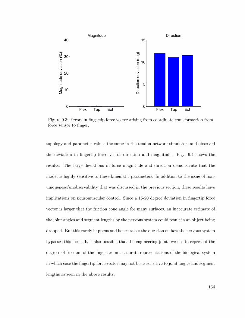
Flex Tap Ext0

10

20

30

40Magnitude

Mag

nitu

de d

evia

tion

(%)

Flex Tap Ext0

5

10

15Direction

Dire

ctio

n de

viat

ion

(deg

)

Figure 9.3: Errors in fingertip force vector arising from coordinate transformation fromforce sensor to finger.

topology and parameter values the same in the tendon network simulator, and observed

the deviation in fingertip force vector direction and magnitude. Fig. 9.4 shows the

results. The large deviations in force magnitude and direction demonstrate that the

model is highly sensitive to these kinematic parameters. In addition to the issue of non-

uniqueness/unobservability that was discussed in the previous section, these results have

implications on neuromuscular control. Since a 15-20 degree deviation in fingertip force

vector is larger that the friction cone angle for many surfaces, an inaccurate estimate of

the joint angles and segment lengths by the nervous system could result in an object being

dropped. But this rarely happens and hence raises the question on how the nervous system

bypasses this issue. It is also possible that the engineering joints we use to represent the

degrees of freedom of the finger are not accurate representations of the biological system

in which case the fingertip force vector may not be as sensitive to joint angles and segment

lengths as seen in the above results.

154

Flex Tap Ext0

25

50Magnitude

Mag

nitu

de d

evia

tion

(%)

Flex Tap Ext0

10

20Direction

Dire

ctio

n de

viat

ion

(deg

)

Figure 9.4: Errors in fingertip force vector arising due to model being an inaccurate rep-resentation of the experimental system. A Monte Carlo analysis shows there is an errorof 25-50 % in fingertip force magnitude and around 15 degrees in force direction arisingfrom a ±5% perturbation in segment lengths and ±5 degrees in joint posture. Thisdemonstrates how sensitive the fingertip force vector is to these kinematic parameters.

9.4 Ambiguity of the Model of the MCP Joint

The kinematics of the MCP joint is still not well understood. Hence there is a larger scope

of error of MCP angle measurement. In addition, the orientation of the ad-abduction axis

with respect to the flexion-extension axis has also been debated. See (Valero-Cuevas 1997)

for a description on different models of the MCP joint. Here, we performed another Monte

Carlo simulation to see how changing the angle between the MCP flexion-extension and

ad-abduction joint axes affected fingertip force vector (Fig. 9.5). We perturbed this

angle between 70 and 100 degrees and observed that the fingertip force vector magnitude

and direction are very sensitive to this parameter. Hence, there is a need to accurately

characterize the kinematic nature of the MCP joint and the orientation of the MCP joint

axes.

155

Flex Tap Ext0

100

200

300Magnitude

Mag

nitu

de d

evia

tion

(%)

Flex Tap Ext0

20

40

Direction

Dire

ctio

n de

viat

ion

(deg

)

Figure 9.5: Sensitivity of fingertip force vector to changes in angle between MCP flexion-extension and ad-abduction axes. The nature of the MCP joint is not clearly under-stood. A Monte Carlo simulation where the angle between the MCP flexion-extensionand the MCP ad-abduction axes was perturbed between 70 and 100 degrees resultedin large fingertip force output deviations thus demonstrating that the fingertip forcevector is very sensitive to this angle parameter.

9.5 Stiffness of the Tendon Network

Unlike muscles, tendons have low compliance. The extensor mechanism is a network of

very stiff collagenous strings that stretch very little. For all the elements of this network

to transmit force upon loading, they need to be connected in a very specific manner

with accurately determined lengths. Otherwise, there is a high chance that part of the

network would go slack and hence not contribute to force transmission. It would also be

interesting to compare the string like representation used in this dissertation to model

the collagenous network of the extensor mechanism, against a sheet like representation.

It is possible that the existence of a large number of fibers in the sheet introduces a

redundancy that allows slackening of some fibers and still allow force transmission.

156

9.6 Implementation in the Clinic

The ultimate goal would be to apply the computational techniques described in this disser-

tation to infer accurate subject-specific models of tendon networks in patients with tendon

injury as well as those with nerve palsies, in the clinic. The main challenge to achieve this

goal is the measurement of forces exerted by the muscles on the tendon networks (or alter-

natively, the tendon excursions produced by muscle contraction/stretching). Currently,

there is no way to infer these quantities accurately in live subjects. While electromyogram

is useful to determine when a particular muscle or group of muscles is on or off, its relation

to muscle force or muscle displacement is not understood(Inman et al. 1952, Disselhorst-

Klug et al. 2009). However, recent technological advances particularly in imaging show

promise that we could, in the near future, be able to measure musculotendon movements

in real-time in live subjects (Blemker et al. 2007). In addition to this, there have also

been studies to infer muscle forces using fluctuations in endpoint force (Kutch, Kuo &

Rymer 2010). Until the technology is available, we will have to settle with generalizable

models that capture behavior across a population. However, it is possible that there ex-

ists a finite number of ‘types’ or ‘classes’ of tendon networks that exist in the population.

This has been shown to be the case with respect to human thumb models as described

in (Santos & Valero-Cuevas 2006). Such classes of tendon networks could be identified

from testing of multiple cadaveric specimens using the inference methods described in

this dissertation.

157

9.7 Acknowledgement

Coauthors Dr. Francisco Valero-Cuevas and Dr. Hod Lipson. NSF Grants EFRI-COPN

0836042 and NIH Grants AR050520 and AR052345 to FVC.

158

Chapter 10

Conclusions and Future Work

In this dissertation, we have presented novel methods for the computational modeling of

musculoskeletal systems. These methods are based on the inference of accurate models

of these systems from sparse experimental data. Using the complex tendon networks of

the human fingers as an example, we have demonstrated the development of two kinds of

computational models – analytical models consisting of functions mapping joint angles

to tendon excursions, and anatomy-based models capturing the interactions of a network

of elastic tendons with the bones of the fingers. We have implemented a novel inference

technique based on symbolic regression to infer mathematical forms and parameter val-

ues of tendon routing in musculoskeletal systems. We showed that the functions inferred

using this method are more accurate, require fewer training data points, have fewer pa-

rameters, are more robust to noise, and can extrapolate better than polynomial regression

models, the state of the art in musculoskeletal modeling. We applied this technique to

learn analytical models modeling the tendon excursions of the human index finger and

showed that these functions are more accurate than Landsmeer-based models or poly-

nomial regressions whether our goal is to obtain subject-specific models or models that

159

generalize across specimens. We successfully controlled a human cadaveric index finger

to produce a slow tapping motion for the first time ever (to the best of our knowledge)

and learned that a spring-based ‘muscle-like’ control was more effective in producing slow

finger motions than simple force or position control. We demonstrated that the finger

has neutral equilibrium in a specific range of postures when the input tendon tensions are

in(or close to) the null space of the moment arm matrix of the finger in those postures.

Stable equilibrium was observed in other postures. We developed a novel finite element

method based tendon network simulator to simulate the interactions of elastic tendon

networks with arbitrarily shaped solids and used this to study the sensitivity of fingertip

force magnitude and direction to the elastic properties and topology of the extensor mech-

anism. We concluded that the output is most sensitive to the resting lengths of the fibers

and the topology of the structure. We then implemented a novel inference algorithm to

infer the three dimensional network structure of the extensor mechanism of the fingers

from minimal experimental data through intelligent testing. The models of the extensor

mechanism inferred more accurately matched with experimental data compared to the

An-Chao normative model used extensively in the literature.

The computational methods developed in this dissertation are a combination of tech-

niques in biomechanics, machine learning and electromechanical experimentation. They

can be used for the inference of accurate models of different musculoskeletal systems in

the body. Analytical models are critical for dynamical simulations especially for control.

The analytical models for the index finger presented here are currently being used as

a representation of the biomechanics of the ‘plant’ to test theories of motor control in

human manipulation. More work needs to be done to see how the nervous system could

160

be using the neutral equilibrium in the fingers observed here and its implications on our

understanding of grasp and manipulation. The tendon network environment developed

here can be a useful tool for clinical research to understand how damage or injury to

the network can affect fingertip force production. The inference of the three dimensional

structure of the finger model demonstrated in this dissertation is a step towards the in-

ference of subject specific models of musculoskeletal systems. Combining it with real

time magnetic resonance or ultrasound imaging could in the future enable development

of individualized models of these systems and to study specific changes on damage or

repair.

161

Bibliography

Abend, W., Bizzi, E. & Morasso, P. (1982), ‘Human arm trajectory formation’, Brain105(Pt 2), 331–48.

An, K., Linscheid, R. & Brand, P. (1991), ‘Correlation of physiological cross-sectional ar-eas of muscle and tendon.’, Journal of hand surgery (Edinburgh, Scotland) 16(1), 66.

An, K. N., Chao, E. Y., Cooney, W. P. & Linscheid, R. L. (1979), ‘Normative model ofhuman hand for biomechanical analysis.’, J Biomech 12(10), 775–788.

An, K. N., Chao, E. Y., Cooney, W. P. & Linscheid, R. L. (1985), ‘Forces in the normaland abnormal hand’, Journal of Orthopaedic Research 3(2).

An, K. N., Chao, E. Y. S. & Kaufman, K. R. (1991), ‘Analysis of muscle and joint loads’,Basic orthopaedic biomechanics pp. 1–50.

An, K. N., Takahashi, K., Harrigan, T. P. & Chao, E. Y. (1984), ‘Determination of muscleorientations and moment arms’, Journal of biomechanical engineering 106, 280.

An, K. N., Ueba, Y., Chao, E. Y., Cooney, W. P. & Linscheid, R. L. (1983), ‘Tendonexcursion and moment arm of index finger muscles’, J Biomech 16(6), 419–25.

Anderson, A. E., Ellis, B. J. & Weiss, J. A. (2007), ‘Verification, validation and sensitivitystudies in computational biomechanics’, Computer methods in biomechanics andbiomedical engineering 10(3), 171–184.

Anderson, F. C. & Pandy, M. G. (2001), ‘Dynamic optimization of human walking’,Journal of biomechanical engineering 123, 381.

Andriacchi, T. P., Natarajan, R. N. & Hurwitz, D. E. (1991), ‘Musculoskeletal dynamics,locomotion, and clinical applications’, Basic orthopaedic biomechanics p. 51.

Bartel, D. L., Bicknell, V. L. & Wright, T. M. (1986), ‘The effect of conformity, thickness,and material on stresses in ultra-high molecular weight components for total jointreplacement’, J Bone Joint Surg Am 68(7), 1041–1051.

Bendz, P. (1985), ‘The functional significance of the oblique retinacular ligament oflandsmeer. a review and new proposals’, The Journal of Hand Surgery: Journalof the British Society for Surgery of the Hand 10(1), 25–29.

Berme, N., Paul, J. P. & Purves, W. K. (1977), ‘A biomechanical analysis of themetacarpo-phalangeal joint’, Journal of Biomechanics 10(7), 409–412.

162

Bernstein, N. (1967), The co-ordination and regulation of movements, Oxford, UK: Perg-amo.

Blankevoort, L., Kuiper, J. H., Huiskes, R. & Grootenboer, H. J. (1991), ‘Articular con-tact in a three-dimensional model of the knee’, Journal of Biomechanics 24(11), 1019.

Blemker, S. S., Asakawa, D. S., Gold, G. E. & Delp, S. L. (2007), ‘Image-based mus-culoskeletal modeling: applications, advances, and future opportunities’, Journal ofMagnetic Resonance Imaging 25(2), 441–451.

Blemker, S. S. & Delp, S. L. (2005), ‘Three-dimensional representation of complex musclearchitectures and geometries’, Annals of Biomedical Engineering 33(5), 661–673.

Bongard, J. C. & Lipson, H. (2004a), Automating genetic network inference with minimalphysical experimentation using coevolution, in ‘Genetic and Evolutionary Compu-tation Conference (GECCO) 2004’, Springer, pp. 333–345.

Bongard, J. C. & Lipson, H. (2005a), ‘Nonlinear system identification using coevolution ofmodels and tests’, Evolutionary Computation, IEEE Transactions on 9(4), 361–384.

Bongard, J. & Lipson, H. (2004b), Once more unto the breach: Co-evolving a robot and itssimulator, in ‘Proceedings of the Ninth International Conference on the Simulationand Synthesis of Living Systems (ALIFE9)’, pp. 57–62.

Bongard, J. & Lipson, H. (2005b), ‘Active coevolutionary learning of deterministic finiteautomata’, The Journal of Machine Learning Research 6, 1651–1678.

Brand, P. W. & Hollister, A. (1999), Clinical mechanics of the hand, Mosby St. Louis,MO.

Brook, N., Mizrahi, J., Shoham, M. & Dayan, J. (1995), ‘A biomechanical model of indexfinger dynamics’, Medical Engineering and Physics 17(1), 54–63.

Brown, I. E. & Loeb, G. E. (2000), ‘A reductionist approach to creating and using neuro-musculoskeletal models’, Biomechanics and Neural Control of Posture and Movementpp. 148–163.

Buchanan, T. S., Lloyd, D. G., Manal, K. & Besier, T. F. (2004), ‘Neuromusculoskeletalmodeling: Estimation of muscle forces and joint moments and movements frommeasurements of neural command’, J Appl Biomech 20(4), 367–395.

Buchner, H. J., Hines, M. J. & Hemami, H. (1988), ‘A dynamic model for finger inter-phalangeal coordination’, J Biomech 21(6), 459–68.

Buford Jr, W. L., Ivey Jr, F. M., Malone, J. D., Patterson, R. M., Pearce, G. L., Nguyen,D. K. & Stewart, A. A. (1997), ‘Muscle balance at the knee-moment arms for thenormal knee and the acl-minus knee’, Rehabilitation Engineering, IEEE Transactionson 5(4), 367–379.

Bunnell, S. (1945), ‘Surgery of the hand’, Southern Medical Journal 38(3), 228.

163

Cappozzo, A., Catani, F., Leardini, A., Benedetti, M. G. & Della Croce, U. (1996), ‘Po-sition and orientation in space of bones during movement: experimental artefacts’,Clinical Biomechanics 11(2), 90–100.

Cerveri, P., De Momi, E., Marchente, M., Lopomo, N., Baud-Bovy, G., Barros, R. M. L. &Ferrigno, G. (2008), ‘In vivo validation of a realistic kinematic model for the trapezio-metacarpal joint using an optoelectronic system’, Annals of Biomedical Engineering36(7), 1268–1280.

Chao, E. (1989), Biomechanics of the hand: a basic research study, World Scientific PubCo Inc.

Chao, E. Y. & An, K. N. (1978a), ‘Determination of internal forces in human hand’,journal of the engineering mechanics division 104(1), 255–272.

Chao, E. Y. & An, K. N. (1978b), ‘Graphical interpretation of the solution to the redun-dant problem in biomechanics’, Journal of Biomechanical Engineering 100, 159–67.

Cheng, E. J., Brown, I. E. & Loeb, G. E. (2000), ‘Virtual muscle: a computationalapproach to understanding the effects of muscle properties on motor control’, Journalof neuroscience methods 101(2), 117–130.

Clavero, J. A., Golano, P., Farinas, O., Alomar, X., Monill, J. M. & Esplugas, M. (2003),‘Extensor mechanism of the fingers: Mr imaging-anatomic correlation 1’, Radio-graphics 23(3), 593–611.

Clewley, R. H., Guckenheimer, J. M. & Valero-Cuevas, F. J. (2008), ‘Estimating effectivedegrees of freedom in motor systems’, IEEE Trans Biomed Eng 55(2 Pt 1), 430–42.

Crisfield, M. A. (1991), Nonlinear finite element analysis of solids and structures. Volume1: Essentials, Wiley, New York, NY (United States).

Damsgaard, M., Rasmussen, J., Christensen, S. T., Surma, E. & de Zee, M. (2006),‘Analysis of musculoskeletal systems in the anybody modeling system’, SimulationModelling Practice and Theory 14(8), 1100–1111.

Darling, W. G., Cole, K. J. & Miller, G. F. (1994), ‘Coordination of index finger move-ments’, Journal of Biomechanics 27(4), 479–491.

Davoodi, R., Brown, I. E. & Loeb, G. E. (2003), ‘Advanced modeling environment for de-veloping and testing fes control systems’, Medical Engineering and Physics 25(1), 3–9.

Davoodi, R. & Loeb, G. E. (2003), A biomimetic strategy for control of fes reaching, in‘Engineering in Medicine and Biology Society, 2003. Proceedings of the 25th AnnualInternational Conference of the IEEE’, Vol. 2. Engineering in Medicine and BiologySociety, 2003. Proceedings of the 25th Annual International Conference of the IEEE.

Davoodi, R., Urata, C., Hauschild, M., Khachani, M. & Loeb, G. E. (2007), ‘Model-based development of neural prostheses for movement’, Biomedical Engineering,IEEE Transactions on 54(11), 1909–1918.

164

Delp, S. L., Anderson, F. C., Arnold, A. S., Loan, P., Habib, A., John, C. T., Guendelman,E. & Thelen, D. G. (2007), ‘Opensim: Open-source software to create and analyzedynamic simulations of movement’, IEEE Trans Biomed Eng 54(11), 1940–1950.

Delp, S. L. & Loan, J. P. (1995), ‘A graphics-based software system to develop andanalyze models of musculoskeletal structures’, Computers in Biology and Medicine25(1), 21–34.

Dennerlein, J. T., Diao, E., Mote Jr, C. D. & Rempel, D. M. (1998), ‘Tensions of theflexor digitorum superficialis are higher than a current model predicts’, Journal ofBiomechanics 31(4), 295–302.

Dennerlein, J. T., Mote Jr, C. D. & Rempel, D. M. (1998), ‘Control strategies for fingermovement during touch-typing the role of the extrinsic muscles during a keystroke’,Experimental Brain Research 121(1), 1–6.

Disselhorst-Klug, C., Schmitz-Rode, T. & Rau, G. (2009), ‘Surface electromyography andmuscle force: Limits in semg-force relationship and new approaches for applications’,Clinical Biomechanics 24(3), 225–235.

Esteki, A. & Mansour, J. (1997), ‘A dynamic model of the hand with application in func-tional neuromuscular stimulation’, Annals of Biomedical Engineering 25(3), 440–451.

Esteki, A. & Mansour, J. M. (1996), ‘An experimentally based nonlinear viscoelasticmodel of joint passive moment’, Journal of Biomechanics 29(4), 443–450.

Fernandez, J. W. & Pandy, M. G. (2006), ‘Integrating modelling and experiments to assessdynamic musculoskeletal function in humans’, Experimental Physiology 91(2), 371–382.

Franko, O., Winters, T., Tirrell, T., Hentzen, E. & Lieber, R. (2011), ‘Moment arms ofthe human digital flexors’, Journal of Biomechanics 44(10), 1987–1990.

Fregly, B. (2008), ‘Computational assessment of combinations of gait modifications forknee osteoarthritis rehabilitation’, Biomedical Engineering, IEEE Transactions on55(8), 2104–2106.

Fuglevand, A. J., Winter, D. A. & Patla, A. E. (1993), ‘Models of recruitment and ratecoding organization in motor-unit pools’, J Neurophysiol 70(6), 2470–88.

Garcia-Elias, M., An, K. N., Berglund, L. J., Linscheid, R. L., Cooney, W. P. & Chao, E.(1991), ‘Extensor mechanism of the fingers. ii. tensile properties of components***’,The Journal of hand surgery 16(6), 1136–1140.

Garcia-Elias, M., An, K. N., Berglund, L., Linscheid, R. L., Cooney Iii, W. P. & Chao,E. (1991), ‘Extensor mechanism of the fingers. i. a quantitative geometric study***’,The Journal of hand surgery 16(6), 1130–1136.

165

Garcia, M., Chatterjee, A., Ruina, A. & Coleman, M. (1998), ‘The simplest walkingmodel: Stability, complexity, and scaling’, ASME Journal of Biomechanical Engi-neering 120, 281–288.

Garner, B. A. & Pandy, M. G. (2000), ‘The obstacle-set method for representing musclepaths in musculoskeletal models’, Computer methods in biomechanics and biomedicalengineering 3(1), 1–30.

Gatti, C. & Hughes, R. (2009), ‘Optimization of muscle wrapping objects using simulatedannealing’, Annals of Biomedical Engineering 37(7), 1342–1347.

Goehler, C. & Murray, W. (2010), ‘The sensitivity of endpoint forces produced by theextrinsic muscles of the thumb to posture’, Journal of biomechanics 43(8), 1553–1559.

Gonzalez, R. V., Hutchins, E. L., Barr, R. E. & Abraham, L. D. (1996), ‘Developmentand evaluation of a musculoskeletal model of the elbow joint complex’, Journal ofbiomechanical engineering 118, 32.

Green, P. J. & Silverman, B. W. (1994), Nonparametric regression and generalized linearmodels: a roughness penalty approach, Vol. 58, Chapman & Hall/CRC.

Haines, R. W. (1951), ‘The extensor apparatus of the finger’, Journal of Anatomy 85(Pt3), 251.

Happee, R. & Van der Helm, F. C. T. (1995), ‘The control of shoulder muscles duringgoal directed movements, an inverse dynamic analysis’, Journal of Biomechanics28(10), 1179–1191.

Harding, D. C., Brandt, K. D. & Hillberry, B. M. (1993), ‘Finger joint force minimizationin pianists using optimization techniques.’, J Biomech 26(12), 1403–1412.

Harris Jr, C. & Rutledge Jr, G. (1972), ‘The functional anatomy of the extensor mecha-nism of the finger’.

Hatze, H. (1977), ‘A myocybernetic control model of skeletal muscle’, Biological Cyber-netics 25(2), 103–119.

Hatze, H. (1997), ‘A three-dimensional multivariate model of passive human joint torquesand articular boundaries’, Clinical Biomechanics 12(2), 128–135.

Hatze, H. (2002), ‘The fundamental problem of myoskeletal inverse dynamics and itsimplications’, Journal of Biomechanics 35(1), 109–115.

Hatze, H. (2005), ‘Towards a comprehensive large-scale computer model of the humanneuromusculoskeletal system’, Theoretical Issues in Ergonomics Science 6(3), 239–250.

Herrmann, A. & Delp, S. (1999), ‘Moment arm and force-generating capacity of theextensor carpi ulnaris after transfer to the extensor carpi radialis brevis’, The Journalof hand surgery 24(5), 1083–1090.

166

Herzog, W. & Read, L. J. (1993), ‘Lines of action and moment arms of the major force-carrying structures crossing the human knee joint’, Journal of Anatomy 182(Pt2), 213.

Holden, J. P., Orsini, J. A., Siegel, K. L., Kepple, T. M., Gerber, L. H. & Stanhope, S. J.(1997), ‘Surface movement errors in shank kinematics and knee kinetics during gait’,Gait & Posture 5(3), 217–227.

Hollister, A., Buford, W. L., Myers, L. M., Giurintano, D. J. & Novick, A. (1992),‘The axes of rotation of the thumb carpometacarpal joint’, Journal of OrthopaedicResearch 10(3), 454–460.

Holzbaur, K. R. S., Murray, W. M. & Delp, S. L. (2005), ‘A model of the upper extremityfor simulating musculoskeletal surgery and analyzing neuromuscular control’, Annalsof Biomedical Engineering 33(6), 829–840.

Hoy, M. G., Zajac, F. E. & Gordon, M. E. (1990), ‘A musculoskeletal model of the humanlower extremity: the effect of muscle, tendon, and moment arm on the moment-anglerelationship of musculotendon actuators at the hip, knee, and ankle’, Journal ofBiomechanics 23(2), 157–169.

Huiskes, R. & Chao, E. Y. (1983), ‘A survey of finite element analysis in orthopedicbiomechanics: the first decade’, Journal of Biomechanics 16(6), 385.

Hull, M. L. & Jorge, M. (1985), ‘A method for biomechanical analysis of bicycle pedaling’,Journal of Biomechanics 18(9), 631–644.

Inman, V., Ralston, H., De CM Saunders, J., Bertram Feinstein, M. & Wright Jr, E.(1952), ‘Relation of human electromyogram to muscular tension’, Electroencephalog-raphy and clinical Neurophysiology 4(2), 187–194.

Inman, V. T. (1944), ‘Observations on the function of the shoulder joint’, The Journal ofBone and Joint Surgery 26(1), 1.

Jinha, A., Ait-Haddou, R., Binding, P. & Herzog, W. (2006), ‘Antagonistic activity ofone-joint muscles in three-dimensions using non-linear optimisation’, Mathematicalbiosciences 202(1), 57–70.

Kamper, D. G., George Hornby, T. & Rymer, W. Z. (2002), ‘Extrinsic flexor mus-cles generate concurrent flexion of all three finger joints’, Journal of Biomechanics35(12), 1581–1590.

Karniel, A. & Inbar, G. F. (1997), ‘A model for learning human reaching movements’,Biological Cybernetics 77(3), 173–183.

Kaufman, K. R., An, K. A., Litchy, W. J. & Chao, E. Y. S. (1991), ‘Physiological predic-tion of muscle forces. ii, application to isokinetic exercise’, Neuroscience 40(3), 793–804.

167

Khang, G. & Zajac, F. E. (1989), ‘Paraplegic standing controlled by functional neuromus-cular stimulation: Part i–computer model and control-system design.’, IEEE TransBiomed Eng 36(9), 873–884.

Koza, J. R. (1992), Genetic programming: On the programming of computers by meansof natural selection, The MIT press, Cambridge, Massachusetts.

Kuo, A. D. (2002), ‘Energetics of actively powered locomotion using the simplest walkingmodel’, Journal of biomechanical engineering 124, 113.

Kuo, A. D. & Maxwell Donelan, J. (2009), ‘Comment on ”contributions of the individualankle plantar flexors to support, forward progression and swing initiation duringwalking” ((neptune et al., 2001) and ”muscle mechanical work requirements duringnormal walking: the energetic cost of raising the body’s center-of-mass is significant”(neptune et al., 2004)’, J Biomech 42(11), 1783–5; author reply 1786–9.

Kuo, P. L., Lee, D. L., Jindrich, D. L. & Dennerlein, J. T. (2006), ‘Finger joint coordi-nation during tapping’, Journal of Biomechanics 39(16), 2934–2942.

Kurse, M., Lipson, H. & Valero-Cuevas, F. J. (2012), ‘Extrapolatable analytical functionsfor tendon excursions and moment arms from sparse datasets’, IEEE Transactionson Biomedical Engineering 59(6), 1572–1582.

Kutch, J., Kuo, A. & Rymer, W. (2010), ‘Extraction of individual muscle mechanicalaction from endpoint force’, Journal of neurophysiology 103(6), 3535–3546.

Kutch, J. & Valero-Cuevas, F. (2011), ‘Muscle redundancy does not imply robustness tomuscle dysfunction’, Journal of Biomechanics 44(7), 1264–1270.

Landsmeer, J. M. (1961), ‘Studies in the anatomy of articulation. i. the equilibrium ofthe” intercalated” bone’, Acta morphologica Neerlando-Scandinavica 3, 287.

Landsmeer, J. M. F. (1949), ‘The anatomy of the dorsal aponeurosis of the human fingerand its functional significance’, The Anatomical Record 104(1).

Landsmeer, J. M. F. (1963), ‘The coordination of finger-joint motions’, The Journal ofBone and Joint Surgery 45(8), 1654.

Lee, J. W. & Rim, K. (1990), ‘Maximum finger force prediction using a planar simula-tion of the middle finger’, ARCHIVE: Proceedings of the Institution of MechanicalEngineers, Part H: Journal of Engineering in Medicine 1989-1996 (vols 203-210)204(38), 169–178.

Lee, S. W., Chen, H., Towles, J. D. & Kamper, D. G. (2008), ‘Estimation of the effectivestatic moment arms of the tendons in the index finger extensor mechanism’, Journalof Biomechanics 41(7), 1567–1573.

Leijnse, J. (1996), ‘A graphic analysis of the biomechanics of the massless bi-articularchain. application to the proximal bi-articular chain of the human finger’, Journalof Biomechanics 29(3), 355–366.

168

Leijnse, J., Bonte, J. E., Landsmeer, J. M. F., Kalker, J. J., Van der Meulen, J. C.& Snijders, C. J. (1992), ‘Biomechanics of the finger with anatomical restrictions–the significance for the exercising hand of the musician’, Journal of Biomechanics25(11), 1253–1264.

Li, Z. M., Zatsiorsky, V. M. & Latash, M. L. (2001), ‘The effect of finger extensormechanism on the flexor force during isometric tasks’, Journal of Biomechanics34(8), 1097–1102.

Lieber, R. L., Jacobson, M. D., Fazeli, B. M., Abrams, R. A. & Botte, M. J. (1992),‘Architecture of selected muscles of the arm and forearm: anatomy and implicationsfor tendon transfer’, The Journal of hand surgery 17(5), 787.

Lipson, H. (2006), ‘A relaxation method for simulating the kinematics of compoundnonlinear mechanisms’, Journal of Mechanical Design 128, 719.

Lipson, H., Bongard, J., Zykov, V. & Malone, E. (2006), Evolutionary robotics for leggedmachines: from simulation to physical reality, in ‘Intelligent Autonomous Systems’,Vol. 9, p. 9.

Littler, J. W. (1967), ‘The finger extensor mechanism’, The Surgical Clinics of NorthAmerica 47(2), 415.

Liu, J., Hughes, R. E., Smutz, W. P., Niebur, G. & Nan-An, K. (1997), ‘Roles of deltoidand rotator cuff muscles in shoulder elevation’, Clinical Biomechanics 12(1), 32–38.

Maganaris, C. N. (2004), ‘Imaging-based estimates of moment arm length in intact humanmuscle-tendons’, European journal of applied physiology 91(2), 130–139.

Magermans, D., Chadwick, E., Veeger, H., Rozing, P. & Van der Helm, F. (2004), ‘Ef-fectiveness of tendon transfers for massive rotator cuff tears: a simulation study’,Clinical Biomechanics 19(2), 116–122.

McLean, S., Su, A. & van den Bogert, A. (2003), ‘Development and validation of a 3-dmodel to predict knee joint loading during dynamic movement’, Journal of biome-chanical engineering 125, 864.

Menegaldo, L. L., de Toledo Fleury, A. & Weber, H. I. (2004), ‘Moment arms and mus-culotendon lengths estimation for a three-dimensional lower-limb model’, Journal ofBiomechanics 37(9), 1447–1453.

Micks, J. E. & Reswick, J. B. (1981), ‘Confirmation of differential loading of lateral andcentral fibers of the extensor tendon’, The Journal of hand surgery 6(5), 462.

Murray, R., Li, Z. & Sastry, S. (1994), A mathematical introduction to robotic manipula-tion, CRC.

Murray, W. M., Delp, S. L. & Buchanan, T. S. (1995), ‘Variation of muscle moment armswith elbow and forearm position’, Journal of Biomechanics 28(5), 513–525.

169

Mussa-Ivaldi, F. A., Hogan, N. & Bizzi, E. (1985), ‘Neural, mechanical, and geometricfactors subserving arm posture in humans’, Journal of Neuroscience 5(10), 2732–2743.

Neptune, R. (2000), ‘Computer modeling and simulation of human movement’, ScientificPrinciples of Sports Rehabilitation 11(2), 417–434.

Neptune, R. R., Kautz, S. A. & Zajac, F. E. (2001), ‘Contributions of the individual ankleplantar flexors to support, forward progression and swing initiation during walking’,Journal of Biomechanics 34(11), 1387–1398.

Neptune, R. R., McGowan, C. P. & Kautz, S. A. (2009), ‘Forward dynamics simulationsprovide insight into muscle mechanical work during human locomotion’, Exerciseand sport sciences reviews 37(4), 203.

Neptune, R. R., Zajac, F. E. & Kautz, S. A. (2004), ‘Muscle mechanical work requirementsduring normal walking: the energetic cost of raising the body’s center-of-mass issignificant’, Journal of Biomechanics 37(6), 817–825.

Olney, S. J., Griffin, M. P., Monga, T. N. & McBride, I. D. (1991), ‘Work and powe in gaitof stroke patients’, Archives of physical medicine and rehabilitation 72(5), 309–314.

Otis, J., Jiang, C., Wickiewicz, T., Peterson, M., Warren, R. & Santner, T. (1994),‘Changes in the moment arms of the rotator cuff and deltoid muscles with abductionand rotation’, The Journal of Bone and Joint Surgery 76(5), 667–676.

Pandy, M. G. (2001), ‘Computer modeling and simulation of human movement’, Annualreview of biomedical engineering 3(1), 245–273.

Pandy, M. G. & Sasaki, K. (1998), ‘A three-dimensional musculoskeletal model of the hu-man knee joint. part 2: analysis of ligament function’, Computer methods in biome-chanics and biomedical engineering 1(4), 265–283.

Pandy, M. G., Sasaki, K. & Kim, S. (1997), ‘A three-dimensional musculoskeletal modelof the human knee joint. part 1: theoretical construction’, Computer methods inbiomechanics and biomedical engineering 1(2), 87–108.

Patriarco, A. G., Mann, R. W., Simon, S. R. & Mansour, J. M. (1981), ‘An evaluationof the approaches of optimization models in the prediction of muscle forces duringhuman gait’, Journal of Biomechanics 14(8), 513.

Piazza, S. J. (2006), ‘Muscle-driven forward dynamic simulations for the study of normaland pathological gait’, Journal of NeuroEngineering and Rehabilitation 3(1), 5.

Piazza, S. J. & Delp, S. L. (2001), ‘Three-dimensional dynamic simulation of total kneereplacement motion during a step-up task’, Journal of biomechanical engineering123, 599.

Pigeon, P., Yahia, L. H. & Feldman, A. G. (1996), ‘Moment arms and lengths of hu-man upper limb muscles as functions of joint angles’, Journal of Biomechanics29(10), 1365–1370.

170

Prilutsky, B. I. & Zatsiorsky, V. M. (2002), ‘Optimization-based models of muscle coor-dination’, Exercise and sport sciences reviews 30(1), 32.

Purves, W. & Berme, N. (1980), ‘Resultant finger joint loads in selected activities’, Jour-nal of Biomedical Engineering 2(4), 285–289.

Raphael, G., Tsianos, G. & Loeb, G. (2010), ‘Spinal-like regulator facilitates control of atwo-degree-of-freedom wrist’, The Journal of Neuroscience 30(28), 9431–9444.

Rawlinson, J. J. & Bartel, D. L. (2002), ‘Flat medial-lateral conformity in total kneereplacements does not minimize contact stresses.’, J Biomech 35(1), 27–34.

Rawlinson, J. J., Furman, B. D., Li, S., Wright, T. M. & Bartel, D. L. (2006), ‘Retrieval,experimental, and computational assessment of the performance of total knee re-placements.’, J Orthop Res 24(7), 1384–1394.

Rockwell, W. B., Butler, P. N. & Byrne, B. A. (2000), ‘Extensor tendon: Anatomy, injury,and reconstruction’, Plastic and Reconstructive Surgery 106(7), 1592.

Rudlof, S. & Koppen, M. (1996), Stochastic hill climbing with learning by vectors of nor-mal distributions, in ‘Proceedings of the First On-line Workshop on Soft Computing,Nagoya Japan’, pp. 60–70.

Rugg, S. G., Gregor, R. J., Mandelbaum, B. R. & Chiu, L. (1990), ‘In vivo momentarm calculations at the ankle using magnetic resonance imaging (mri)’, Journal ofBiomechanics 23(5), 495–497, 499–501.

Salsbury, C. (1937), ‘The interosseous muscles of the hand’, Journal of Anatomy 71(Pt3), 395.

Sancho-Bru, J. L., Perez-Gonzalez, A., Vergara-Monedero, M. & Giurintano, D. (2001),‘A 3-d dynamic model of human finger for studying free movements’, Journal ofBiomechanics 34(11), 1491–1500.

Sancho-Bru, J., Perez-Gonzalez, A., Vergara, M. & Giurintano, D. (2003), ‘A 3d biome-chanical model of the hand for power grip’, Journal of biomechanical engineering125, 78.

Santello, M., Flanders, M. & Soechting, J. F. (2002), ‘Patterns of hand motion duringgrasping and the influence of sensory guidance’, J Neurosci 22(4), 1426–35. Santello,Marco Flanders, Martha Soechting, John F NS-15018/NS/NINDS NIH HHS/UnitedStates Clinical Trial Research Support, U.S. Gov’t, P.H.S. United States The Journalof neuroscience : the official journal of the Society for Neuroscience J Neurosci. 2002Feb 15;22(4):1426-35.

Santos, V. J., Bustamante, C. D. & Valero-Cuevas, F. J. (2009), ‘Improving the fitnessof high-dimensional biomechanical models via data-driven stochastic exploration’,IEEE Transactions on Biomedical Engineering 56(3).

171

Santos, V. J. & Valero-Cuevas, F. J. (2006), ‘Reported anatomical variability naturallyleads to multimodal distributions of denavit-hartenberg parameters for the humanthumb’, IEEE Trans Biomed Eng 53, 155–163.

Sarrafian, S. K., Kazarian, L. E., Topouzian, L. K., Sarrafian, V. K. & Siegelman, A.(1970), ‘Strain variation in the components of the extensor apparatus of the fingerduring flexion and extension: A biomechanical study’, The Journal of Bone andJoint Surgery 52(5), 980.

Schieber, M. H. & Santello, M. (2004), ‘Hand function: peripheral and central constraintson performance’, Journal of Applied Physiology 96(6), 2293.

Schmidt, M. D. & Lipson, H. (2006), ‘Co-evolving fitness predictors for accelerating andreducing evaluations’, Genetic Programming Theory and Practice IV 5.

Schmidt, M. & Lipson, H. (2005), ‘Coevolution of fitness maximizers and fitness predic-tors’, GECCO Late Breaking Paper .

Schmidt, M. & Lipson, H. (2009), ‘Distilling free-form natural laws from experimentaldata’, science 324(5923), 81.

Schutte, L. M., Rodgers, M. M., Zajac, F. E., Glaser, R. M., Center, V. A. M. & Alto,P. (1993), ‘Improving the efficacy of electrical stimulation-induced leg cycleergome-try: an analysis based on a dynamic musculoskeletal model’, IEEE Transactions onRehabilitation Engineering 1(2), 109–125.

Scott, S. H. (2004), ‘Optimal feedback control and the neural basis of volitional motorcontrol’, Nature Reviews Neuroscience 5(7), 532–546.

Scovil, C. & Ronsky, J. (2006), ‘Sensitivity of a hill-based muscle model to perturbationsin model parameters’, Journal of Biomechanics 39(11), 2055–2063.

Shadmehr, R. & Mussa-Ivaldi, F. A. (1994), ‘Adaptive representation of dynamics duringlearning of a motor task’, Journal of Neuroscience 14(5), 3208–3224.

Smith, R. J. (1974), ‘Balance and kinetics of the fingers under normal and pathologicalconditions’, Clinical orthopaedics and related research 104, 92.

Soechting, J. F. & Flanders, M. (1997), ‘Evaluating an integrated musculoskeletal modelof the human arm’, Journal of biomechanical engineering 119, 93.

Spoor, C. W. (1983), ‘Balancing a force on the fingertip of a two-dimensional finger modelwithout intrinsic muscles’, Journal of Biomechanics 16(7), 497–504.

Spoor, C. W. & Landsmeer, J. M. F. (1976), ‘Analysis of the zigzag movement of thehuman finger under influence of the extensor digitorum tendon and the deep flexortendon’, Journal of Biomechanics 9(9), 561–566.

Spoor, C. W., Van Leeuwen, J. L., Meskers, C. G. M., Titulaer, A. F. & Huson, A.(1990), ‘Estimation of instantaneous moment arms of lower-leg muscles’, Journal ofBiomechanics 23(12), 1247–1259.

172

Stark, H. H., Boyes, J. H. & Wilson, J. N. (1962), ‘Mallet finger’, The Journal of Boneand Joint Surgery 44(6), 1061.

Stern Jr, J. T. (1971), ‘Investigations concerning the theory of ’spurt’ and ’shunt’ muscles’,Journal of Biomechanics 4(5), 437–453.

Sueda, S., Kaufman, A. & Pai, D. K. (2008), ‘Musculotendon simulation for hand ani-mation’, ACM Transactions on Graphics 27(3).

Thelen, D. G., Anderson, F. C. & Delp, S. L. (2003), ‘Generating dynamic simulations ofmovement using computed muscle control’, Journal of Biomechanics 36(3), 321–328.

Theodorou, E., Todorov, E. & Valero-Cuevas, F. J. (2011), Neuromuscular stochastic op-timal control of a tendon driven index finger model, in ‘American Control Conference(ACC), 2011’, pp. 348–355.

Todorov, E. (2007), ‘Probabilistic Inference of Multijoint Movements, Skeletal Parametersand Marker Attachments From Diverse Motion Capture Data’, IEEE Trans BiomedEng 54(11), 1927–1939.

Valero-Cuevas, F. (1997), Muscle coordination of the human index finger, PhD thesis,Doctoral Dissertation, Stanford University, Stanford, CA.

Valero-Cuevas, F. (2000a), Applying principles of robotics to understand the biomechan-ics, neuromuscular control and clinical rehabilitation of human digits, in ‘Roboticsand Automation, 2000. Proceedings. ICRA’00. IEEE International Conference on’,Vol. 1, IEEE, pp. 270–275.

Valero-Cuevas, F. & Hentz, V. (2002), ‘Releasing the a3 pulley and leaving flexor su-perficialis intact increases pinch force following the zancolli lasso procedures to pre-vent claw deformity in the intrinsic palsied finger’, Journal of orthopaedic research20(5), 902–909.

Valero-Cuevas, F., Hoffmann, H., Kurse, M., Kutch, J. & Theodorou, E. (2009), ‘Com-putational models for neuromuscular function’, IEEE Reviews in Biomedical Engi-neering 2, 110.

Valero-Cuevas, F. J. (2000b), ‘Predictive modulation of muscle coordination pattern mag-nitude scales fingertip force magnitude over the voluntary range’, J Neurophysiol83(3), 1469–79.

Valero-Cuevas, F. J. (2005), ‘An integrative approach to the biomechanical function andneuromuscular control of the fingers’, J Biomech 38(4), 673–84.

Valero-Cuevas, F. J. (2009), ‘A mathematical approach to the mechanical capabilities oflimbs and fingers’, Adv. Exp. Med. Biol. 629, 619–633.

Valero-Cuevas, F. J., Anand, V. V., Saxena, A. & Lipson, H. (2007), ‘Beyond parameterestimation: extending biomechanical modeling by the explicit exploration of modeltopology’, IEEE Trans Biomed Eng 54(11), 1951–64.

173

Valero-Cuevas, F. J., Johanson, M. E. & Towles, J. D. (2003), ‘Towards a realistic biome-chanical model of the thumb: the choice of kinematic description may be morecritical than the solution method or the variability/uncertainty of musculoskeletalparameters’, J Biomech 36, 1019–1030.

Valero-Cuevas, F. J. & Lipson, H. (2004), A computational environment to simulate com-plex tendinous topologies, in ‘Conf Proc IEEE Eng Med Biol Soc’, Vol. 6, pp. 4653–6.

Valero-Cuevas, F. J., Towles, J. D. & Hentz, V. R. (2000), ‘Quantification of fingertipforce reduction in the forefinger following simulated paralysis of extensor and intrinsicmuscles’, J Biomech 33(12), 1601–9.

Valero-Cuevas, F. J., Yi, J. W., Brown, D., McNamara, R. V., r., Paul, C. & Lipson, H.(2007), ‘The tendon network of the fingers performs anatomical computation at amacroscopic scale’, IEEE Trans Biomed Eng 54(6 Pt 2), 1161–6.

Valero-Cuevas, F. J., Zajac, F. E. & Burgar, C. G. (1998), ‘Large index-fingertip forcesare produced by subject-independent patterns of muscle excitation’, J Biomech31(8), 693–703.

Van der Helm, F. C. T. (1994), ‘A finite element musculoskeletal model of the shouldermechanism’, Journal of Biomechanics 27(5), 551–559.

Van Langelaan, E. J. (1983), ‘A kinematical analysis of the tarsal joints. an x-ray pho-togrammetric study’, Acta orthopaedica Scandinavica. Supplementum 204, 1.

Van Zuylen, E. J., Van Velzen, A. & van der Gon, J. J. (1988), ‘A biomechanical modelfor flexion torques of human arm muscles as a function of elbow angle’, Journal ofBiomechanics 21(3), 183–190.

Venkadesan, M. & Valero-Cuevas, F. J. (2008), ‘Neural control of motion-to-force transi-tions with the fingertip’, J Neurosci 28(6), 1366–73.

Vigouroux, L., Quaine, F., Labarre-Vila, A. & Moutet, F. (2006), ‘Estimation of fingermuscle tendon tensions and pulley forces during specific sport-climbing grip tech-niques’, Journal of Biomechanics 39(14), 2583–2592.

Visser, J. J., Hoogkamer, J. E., Bobbert, M. F. & Huijing, P. A. (1990), ‘Length and mo-ment arm of human leg muscles as a function of knee and hip-joint angles’, Europeanjournal of applied physiology and occupational physiology 61(5), 453–460.

Weightman, B. & Amis, A. A. (1982), ‘Finger joint force predictions related to design ofjoint replacements’, Journal of Biomedical Engineering 4(3), 197–205.

Winter, D. A. (1990), Biomechanics and motor control of human movement, Wiley-Interscience.

Winters, J. M. (2000), ‘Terminology and foundations of movement science’, Biomechanicsand Neural Control of Posture and Movement p. 3.

174

Wismans, J., Veldpaus, F., Janssen, J., Huson, A. & Struben, P. (1980), ‘A three-dimensional mathematical model of the knee-joint’, Journal of Biomechanics13(8), 677.

Woltring, H. J., Huiskes, R. & de Lange, A. (1983), Measurement error influence on heli-cal axis accuracy in the description of 3d finite joint movement in biomechanics, in‘Proceedings of the American Society of Mechanical Engineers Biomechanics Sympo-sium’, Proceedings of the American Society of Mechanical Engineers BiomechanicsSymposium, Houston, Texas, June, pp. 19–22.

Yamaguchi, G. T. (2005), Dynamic modeling of musculoskeletal motion: a vectorizedapproach for biomechanical analysis in three dimensions, Springer Verlag.

Yeo, S., Mullens, C., Sandercock, T., Pai, D. & Tresch, M. (2011), ‘Estimation of muscu-loskeletal models from in situ measurements of muscle action in the rat hindlimb’,Journal of Experimental Biology 214(5), 735–746.

Yeo, S., Tresch, M. & Pai, D. (2008), Optimal design of musculoskeletal models usingforce field data, in ‘Engineering in Medicine and Biology Society, 2008. EMBS 2008.30th Annual International Conference of the IEEE’, IEEE, pp. 3710–3714.

Yoon, Y. S. & Mansour, J. M. (1982), ‘The passive elastic moment at the hip’, Journalof Biomechanics 15(12), 905.

Yoshikawa, T. (1990), Foundations of robotics: analysis and control, The MIT Press.

Youm, Y., Gillespie, T., Flatt, A. & Sprague, B. (1978), ‘Kinematic investigation ofnormal mcp joint’, Journal of Biomechanics 11(3), 109–118.

Zahalak, G. I. & Ma, S. P. (1990), ‘Muscle activation and contraction: constitutive rela-tions based directly on cross-bridge kinetics’, Journal of biomechanical engineering112, 52.

Zajac, F. E. (1992), ‘How musculotendon architecture and joint geometry affect the ca-pacity of muscles to move and exert force on objects: a review with application toarm and forearm tendon transfer design.’, J Hand Surg Am 17(5), 799–804.

Zajac, F. E. (2002), ‘Understanding muscle coordination of the human leg with dynamicalsimulations’, Journal of Biomechanics 35(8), 1011–1018.

Zajac, F. E., Biosci, J., Physiol, J. C., Biol, J. E., Physiol, Z. V., Lond, J. Z., Physiol,Z. J., Soc, J. G. E., Acta, B. B. & Biochem, A. (1989), ‘Muscle and tendon: proper-ties, models, scaling, and application to biomechanics and motor control’, Crit RevBiomed Eng 17, 359–411.

Zajac, F. E., Neptune, R. R. & Kautz, S. A. (2002), ‘Biomechanics and muscle coordi-nation of human walking part i: introduction to concepts, power transfer, dynamicsand simulations’, Gait and Posture 16(3), 215–232.

175

Zancolli, E. (1979), Structural and dynamic bases of hand surgery, 2nd edn, Lippincott,Philadelphia.

Zdravkovic, V., Jacob, H. & Sennwald, G. (1995), ‘Physical equilibrium of the normalwrist and its relation to clinically defined’, The Journal of Hand Surgery: Journalof the British Society for Surgery of the Hand 20(2), 159–164.

176