INF5820 – 2011 fall Natural Language Processing

INF5830 – 2015 FALL NATURAL LANGUAGE PROCESSING

Jan Tore Lønning, Lecture 12, 2.11

1

Today

Feature selection 1(Oblig 2) Scikit-Learn from NLTK Linear classifiers Naive Bayes is log linear Logistic Regression Multinomial Logistic Regression =

Maximum Entropy Classifiers

2

Machine Learning 3

Data Features Machine Learning Algorithm

Selecting Cleaning Tokenization Lemmatizing? ‘‘Munging’’ …

Feature Selection Arguably the most important step for the results

Example: Word Sense Disambiguation 4

‘‘Bag of words’’-features Features: [fishing, big, sound, player, fly, rod, pound,

double, runs, playing, guitar, band] The example: [0,0,0,1,0,0,0,0,0,0,1,0] Which words as features? How many?

NLTK, initially: The most frequent ones There might be better ways to select (we return to this later)

An electric guitar and bass player stand off to one side, not really part of the scene, just as a sort of nod to gringo expectations perhaps.

• Many features • Boolean values

Hard-line-serve 5

Number of word features

Hard

0 0.802

10 0.768

20 0.764

50 0.774

100 0.800

200 0.812

500 0.830

1000 0.842

2000 0.846

5000 0.844

Hard-line-serve 6


Hard Serve

0 0.802 0.350

10 0.768 0.550

20 0.764 0.622

50 0.774 0.692

100 0.800 0.728

200 0.812 0.766

500 0.830 0.784

1000 0.842 0.794

2000 0.846 0.802

5000 0.844 0.804

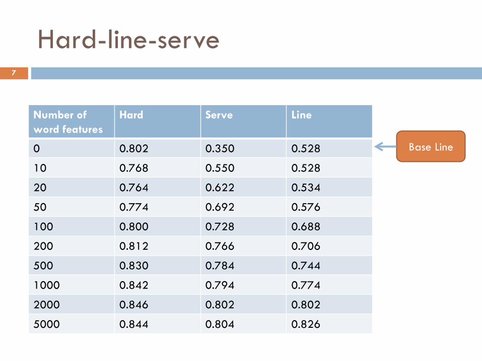
Hard-line-serve 7


Hard Serve Line

0 0.802 0.350 0.528

10 0.768 0.550 0.528

20 0.764 0.622 0.534

50 0.774 0.692 0.576

100 0.800 0.728 0.688

200 0.812 0.766 0.706

500 0.830 0.784 0.744

1000 0.842 0.794 0.774

2000 0.846 0.802 0.802

5000 0.844 0.804 0.826

Base Line

Collocational features 8

With tags: [wi−2,POSi−2,wi−1,POSi−1,wi+1, POSi+1,wi+2, POSi+2] Example: [guitar, NN, and, CC, player, NN, stand, VB]

Without tags: [wi−2,wi−1,wi+1,wi+2] Example: [guitar, and, player, stand]

An electric guitar and bass player stand off to one side, not really part of the scene, just as a sort of nod to gringo expectations perhaps.

• Few features • Many possible values

Window size (without tags) 9

Words on each side

Hard Serve Line

0 0.802 0.350 0.528

1 0.898 0.742 0.734

2 0.886 0.818 0.772

3 0.868 0.856 0.776

4 0.864 0.856 0.782

5 0.854 0.858 0.768

Base Line

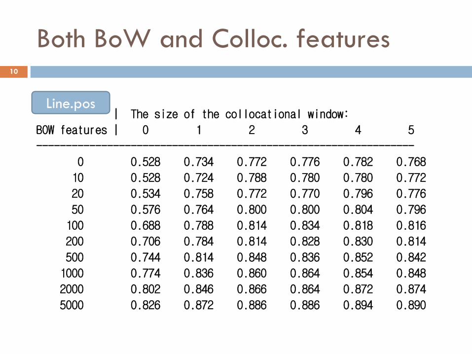
Both BoW and Colloc. features 10

| The size of the collocational window:

BOW features | 0 1 2 3 4 5

----------------------------------------------------------------

0 0.528 0.734 0.772 0.776 0.782 0.768

10 0.528 0.724 0.788 0.780 0.780 0.772

20 0.534 0.758 0.772 0.770 0.796 0.776

50 0.576 0.764 0.800 0.800 0.804 0.796

100 0.688 0.788 0.814 0.834 0.818 0.816

200 0.706 0.784 0.814 0.828 0.830 0.814

500 0.744 0.814 0.848 0.836 0.852 0.842

1000 0.774 0.836 0.860 0.864 0.854 0.848

2000 0.802 0.846 0.866 0.864 0.872 0.874

5000 0.826 0.872 0.886 0.886 0.894 0.890

Line.pos

Today



11

Other ML algorithms in NLTK 12

Included: Naive Bayes (Bernoulli) Decision trees

Import from Scikit-Learn Example: from sklearn.linear_model import LogisticRegression sk_classifier = SklearnClassifier(LogisticRegression()) sk_classifier.train(train_set)

Instead of: classifier = nltk.NaiveBayesClassifier.train(train_set)

Then use the same set-up as in the oblig

Scikit-Learn 13

A large set of various ML classification algorithms They can be imported into NLTK

In general faster than NLTK’s algorithms Beware how the features are selected/formulated:

They may be reformulated/altered when translated into Scikit

Example: SklearnClassifier(BernoulliNB()) performed inferior to

nltk.NaiveBayesClassifier when we used the NLTK-features

Today



14

Geometry: lines

Descartes (1596-1650)

Line: ax + by + c = 0 If b ≠ 0:

y= mx + n n = - c/b is

the intercept with the y-axis

m = -a/b is the slope A point =

intersection of two lines

y = - 2x + 5 4x + 2y – 10 = 0

Normal vector of a line

cos(π/2) = 0 If P passes through

(0,0) there is an n = (xn, yn) s.t.

(x,y) is on P iff (x,y) • (xn, yn) = 0 x × xn = - y × yn

If (a,b) ≠ (0,0) is on P: n = s ×(b, -a) for some

s

Example: y = -2x/5 2x + 5y = 0 (x,y) • (2,5) = 0

Lines not through (0,0)

y = - 2x + 5 2x + y – 5 = 0 (x,y) • (2,1) = 5

Geometry: planes

Plane: ax + by + cz + d = 0 If c ≠ 0:

z= mx + ny + n A line is

the intersection of two planes

3x + 2y –z +2 = 0 z = 3x + 2y + 2

http://www.univie.ac.at/future.media/moe/galerie/geom2/geom2.html#eb

Normal vector of a plane

All points (x,y,z) where ((x,y,z)-(x0,y0,z0))•(a,b,c) =0 (x,y,z) • (a,b,c) = d

(d = a x0+b y0+c z0)

Hyperplane w0+w1x1+w2x2 +… +wnxn = 0 (w1,w2,…,wn) •(x1, x2,…xn)=-w0

Sometimes (n+1 dimensions): (w0,w1,w2,…,wn) •(1,x1, x2,…xn)= 0

Hyperplanes

Generalizes to higher dimensions In n-dimensional space (x1, x2, …, xn):

Points satisfying:

w0 + w1x1 + w2x2 +… + wnxn = 0 for any choice of w0, w1, w2,… wn where not all of w1, w2,… wn = 0

is called a hyper-plane (In machine learning) the same as the intersection of two

hyper-planes in n+1 dimensional space: w0x0 + w1x1 + w2x2 +… + wnxn x0 = 1

Linear classifiers

Assume: All features are numerical

(including Boolean) Two classes

The two classes are linearly separable if they can be separated by a hyperplane

In 2 dimensions that is a line: ax + by < c for red points ax + by > c for blue points

21

Linear classifiers

A linear classifier introduces a hyperplane and classifies accordingly

(If the data aren’t linearly separable, the classifier will make mistakes).

22

Linear classifiers – general case

Try to separate the classes by a hyperplane

(equivalently

taking w0=-θ and x0=1)

The object represented by is in C if and only if

and in –C if

( )nxxx ,...,, 21

∑=

=M

iii xw

1θ

∑=

==•M

iii xwxw

00

∑=

<M

iii xw

1θ

∑=

>M

iii xw

1θ

23

Today



24

Naive Bayes is a log linear classifier

{ }∏=∈

=n

jj

ccccfPcPc

1,)|()(maxargˆ

21

∏∏==

>n

jj

n

jj cfPcPcfPcP

122

111 )|()()|()(

1)|()(

)|()(

122

111

>

∏

∏

=

=n

jj

n

jj

cfPcP

cfPcP

1)|()|(

)()(

1 2

1

2

1 >∏=

n

j j

j

cfPcfP

cPcP

0)|()|(

)()(log

1 2

1

2

1 >

∏=

n

j j

j

cfPcfP

cPcP

0)|()|(

log)()(log

1 2

1

2

1 >

+

∑=

n

j j

j

cfPcfP

cPcP

∑=

=M

iii xw

1θ

=

)|()|(

log2

1

cfPcfP

wj

jj

−=−=

)()(log

2

10 cP

cPwθ

25

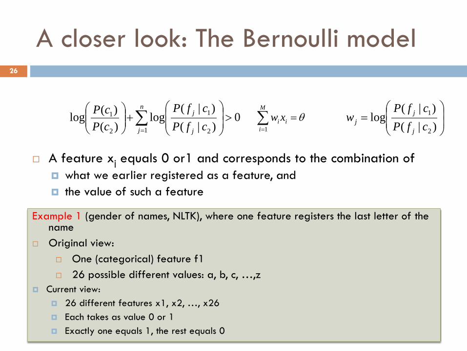
A closer look: The Bernoulli model

A feature xj equals 0 or1 and corresponds to the combination of what we earlier registered as a feature, and the value of such a feature

0)|()|(

log)()(log

1 2

1

2

1 >

+

∑=

n

j j

j

cfPcfP

cPcP ∑

=

=M

iii xw

1θ

=

)|()|(

log2

1

cfPcfP

wj

jj

Example 1 (gender of names, NLTK), where one feature registers the last letter of the name

Original view: One (categorical) feature f1 26 possible different values: a, b, c, …,z

Current view: 26 different features x1, x2, …, x26 Each takes as value 0 or 1 Exactly one equals 1, the rest equals 0

26

A closer look: The Bernoulli model

A feature xj equals 0 or1 and corresponds to the combination of what we earlier registered as a feature, and the value of such a feature

Example 2: text categorization: Original view: one feature fi for a term ti:

fi = 1 if ti is present, fi = 0 if ti isn’t present Current view

one term x2i corresponding to ti being present and one term x2i+1 corresponding to ti being absent

One of these equals 1, the other equals 0

0)|()|(

log)()(log

1 2

1

2

1 >

+

∑=

n

j j

j

cfPcfP

cPcP ∑

=

=M

iii xw

1θ

=

)|()|(

log2

1

cfPcfP

wj

jj

27

A closer look: the multinomial model

The multinomial does not strictly fit the NB-model:

But it fits the linear model If j is the index of a feature term (lexeme) tj (not a particular

occurrence in a document) xj is the number of occurrrences of tj in the document and wj is

0)|()|(

log)()(log

1 2

1

2

1 >

+

∑=

n

j j

j

cfPcfP

cPcP

∑=

=M

jijj xw θ

=

)|()|(

log2

1

cfPcfP

wj

jj

28

Today



29

NB and logistic regression

The NB uses a linear expression to decide

where

Are these the best choices for the wjs? Logistic regression instead faces the question directly: Which wjs make the best classifier of the form

0)|(1

)|(log)|()|(log

100

01

1

2

1 >+==•=

−=

∑∑==

M

iii

M

iii xwxwxwfw

fcPfcP

fcPfcP

=

)|()|(

log2

1

cfPcfP

wj

jj

( ) 0)|(1

)|(ln)|(logit1

0001

11 >+==•=

−= ∑∑

==

M

iii

M

iii xwxwxwfw

fcPfcPfcP

30

Logistic regression – learning

Conditional maximum likelihood estimation: Choose the model that fits the training data best!

where: There are m many training data ci is the class of observation i, i.e. c1 or c2. The feature vector for observation i is:

∑∏==

==m

i

ii

w

m

i

ii

wfcPfcPw

11

)|(logmaxarg)|(maxargˆ

),...,( 21i

niii ffff =

31

There is no analytic solution to

Use some numeric method which runs through a series of iterations e.g. gradient ascent (hill climbing)

There are partial derivatives (gradient) which points out the direction of the ascent

There is a global optimum: convergence But we cannot predict how far to go.

There is a tendency to overfitting, hence regularization

Don’t try this at home! Use a package

Learning algorithms

∑=

=m

i

ii

wfcPw

1)|(logmaxargˆ

fwe

fcP

•−+=

11)|( 1

)()|(logmaxargˆ1

wRfcPwm

i

ii

wα−= ∑

=

where

33

Gradient ascent 34

Today



35

A slight reformulation

We saw that for NB

iff

This could also be written

0)|()|(

log)()(log

1 2

1

2

1 >

+

∑=

n

j j

j

cfPcfP

cPcP

( ) ( ) 0)2|(log)|(log)(log)(log1

121 >−+− ∑=

n

jjj cfPcfPcPcP

∑∑==

+>+n

jj

n

jj cfPcPcfPcP

12

111 )2|(log)(log)|(log)(log

)|()|( 21 fcPfcP

> ∏∏==

>n

jj

n

jj cfPcPcfPcP

122

111 )|()()|()(

36

Reformualtion, contd. 37

has the form where

and our earlier

So the probability in this notation

and similarly for P(c2|f)

∑∑==

+>+n

jj

n

jj cfPcPcfPcP

12

111 )2|(log)(log)|(log)(log

fwxwxwfwM

iii

M

iii

•=>=• ∑∑

==

2

0

2

0

11

))|(log( 11 cfPw jj =

21jjj www −=

))|(log( 22 cfPw jj =

fwfw

fw

fww

fww

fw

fw

eee

ee

eefcP

••

•

•−

•−

•

•

+=

+=

+= 12

1

21

21

)(

)(

1 11)|(

Multinomial logistic regression

We may generalize this to more than two classes For each class cj for j = 1,..,k a linear expression and the probability of belonging to class cj:

where

and

( ) ∏ ∏=

=∑==•= •

i i

fi

fwfwjj i

ifjii i

jij

aZ

wZ

eZ

eZ

fwZ

fcP e 1111exp1)|(

jiw

i ea =

( )∑=

•=k

j

j fwZ1exp

∑=

=•M

ii

ji

j xwfw0

classifierlinear as NBBinary )(Bernoulli Bayes Naive

regression Logisticregression lMultinomia

≈

38

Footnote: Alternative formulation

(In case you read other presentations, like Mitchell or Hastie et. al.: They use a slightly different formulation, corresponding to

where for i = 1, 2,…, k-1:

But and

The two formulations are equivalent though: In the J&M formulation, divide the numerator and denominator in each P(ci|f)

with

and you get this formulation (with adjustments to Z and w.)

( )∑−

=

•+=1

1exp1

k

i

i fwZ

( )∑−

=

•+= 1

1exp1

1)|( k

i

i

k

fwfcP

( ) ∏ ∏=

=∑==•= •

j j

fj

fwfwii j

jfijj j

iji

aZ

wZ

eZ

eZ

fwZ

fcP e 1111exp1)|(

( )fwk

•exp

39

Indicator variables

Already seen: categorical variables represented by indicator variables, taking the values 0,1

Also usual to let the variables indicate both observation and class

( ) ( )( ) ∑ ∑

∑

∑ ∑

∑

∑= =

=

= =

=

=

=

=•

•=•=

k

l

li

m

ii

ji

m

ii

k

li

n

i

li

i

n

i

ji

k

l

l

jjj

xcfw

xcfw

fw

fw

fw

fwfwZ

fcP

1 0

0

1 0

0

1),(exp

),(exp

exp

exp

exp

expexp1)|(

40

Examples – J&M 41

Why called ”maximum entropy”?

See NLTK book for a further example

42

P(NN)+P(JJ)+P(NNS)+P(VB)=1

P(NN)+P(NNS)=0.8

P(VB)=1/20

Why called ”maximum entropy”?

The multinomial logistic regression yields the probability distribution which Gives the maximum entropy Given our training data

43

Learning

Similarly to the binary logistic regression, Regularization

NLTK: Some iterative optimization techniques are much faster than others.

When training Maximum Entropy models, avoid the use of Generalized Iterative Scaling (GIS) or Improved Iterative Scaling (IIS),

which are both considerably slower than the Conjugate Gradient (CG) and the BFGS optimization methods.

44

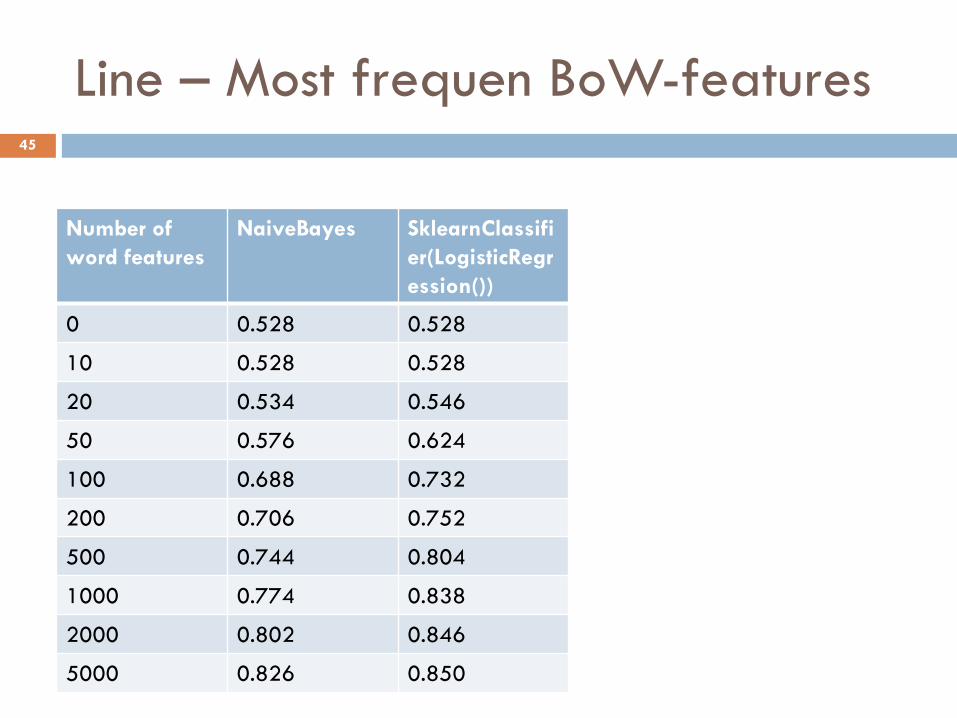
Line – Most frequen BoW-features 45


NaiveBayes SklearnClassifier(LogisticRegression())

0 0.528 0.528

10 0.528 0.528

20 0.534 0.546

50 0.576 0.624

100 0.688 0.732

200 0.706 0.752

500 0.744 0.804

1000 0.774 0.838

2000 0.802 0.846

5000 0.826 0.850

INF5820 – 2011 fall Natural Language Processing

Documents

Transcript of INF5820 – 2011 fall Natural Language Processing