Working Paper Series

Inequality of opportunity and growth Gustavo A. Marrero Juan G. Rodríguez

ECINEQ WP 2010 – 154

ECINEQ 2010-154

February 2010

www.ecineq.org

Inequality of opportunity and growth*

Gustavo A. Marrero Universidad de La Laguna

Juan G. Rodríguez†

Universidad Rey Juan Carlos

Abstract Theoretical and empirical studies exploring the effects of income inequality upon growth reach a disappointing inconclusive result. This paper postulates that one reason for this ambiguity is that income inequality is actually a composite measure of at least two different sorts of inequality: inequality of opportunity and inequality of returns to effort. These two types of inequality affect growth through opposite channels, so the relationship between income inequality and growth is positive or negative depending on which component is larger. We test this proposal using inequality-of-opportunity measures computed from the PSID database for 23 states of the U.S. in 1980 and 1990. We find robust support for a negative relationship between inequality of opportunity and growth, and a positive relationship between inequality of returns to effort and growth. Keywords: income inequality; inequality of opportunity; economic growth. JEL Classification: D63, E24, O15, O40.

* We are grateful for assistance with the data base from Marta Huerta and Elijah Baley. We also acknowledge helpful comments and suggestions of François Bourguignon, John Roemer, Francisco Ferreira, Shlomo Yitzhaki and the audiences at ECINEQ2009 (Buenos Aires), XXXIV Simposio de la Asociación Española de Economía (Valencia), XII Encuentro de Economía Aplicada (Madrid) and FEDEA (Madrid). This paper has benefited from the support of the Spanish Ministry of Education and Science [Project SEJ2006-15172/ECON and SEJ2006-14354/ECON]. The usual disclaimer applies. † Address of correspondence: G. Marrero, Departamento de Análisis Económico (Universidad de La

Laguna, Spain), FEDEA, ICAE and CAERP. Tel: +34 985 103768. E-mail: gmarrero@ull.es. J. G. Rodriguez, Instituto de Estudios Fiscales and Departamento Economía Aplicada I (Universidad Rey Juan Carlos, Spain). Tel: +34 91 4888031. E-mail: juangabriel.rodriguez@urjc.es

2

1. Introduction

A surge of literature on income inequality and growth has emerged over the last two

decades.2 On one hand, this literature addresses the causation from growth to inequality,

and disputes about the Kuznets (1955) and the “augmented” Kuznets hypothesis

(Milanovic, 1994), according to which economic development (and other socio-

economic and political aspects) should eventually reduce income inequality. On the

other hand, the reverse causation is studied, i.e., the effects of income inequality on

growth. We concentrate on this second channel of influence, whose related literature has

lead to controversial conclusions.

The analysis of the relationship between inequality and growth suggests many

channels through which inequality can affect growth. Accumulation of savings

(Galenson and Leibenstein, 1955), unobservable effort (Mirrless, 1971), and the

investment project size (Barro, 2000) are some of the main routes through which

inequality may enhance growth. On the contrary, inequality can negatively affect

growth through the following channels: unproductive investments (Mason, 1988), levels

of nutrition and health (Dasgupta and Ray, 1987), demand patterns (Marshall, 1988),

capital market imperfections (Banerjee and Newman, 1991), fertility (Galor and Zang,

1997), domestic market size (Murphy et al., 1989), political economy (Persson and

Tabellini, 1994), and political instability (Alesina and Perotti, 1996). Thus, overall

inequality would affect growth positively or negatively depending on the channels that

dominate.

However, the existing empirical literature does not indicate that any of these

channels has a predominant influence. As a result, the relationship between inequality

2 Surveys on this issue can be found in Bénabou (1996), Bourguignon (1996), Aghion et al. (1999),

Bertola et al. (2005) and Ehrhart (2009).

3

and growth turns out to be ambiguous.3 Empirical papers tend to justify this ambiguity

through the quality of data (Deininger and Squire, 1996), the inconsistent nature of

inequality measures (Knowles, 2001), the type of inequality index (Székely, 2003), the

econometric method (Forbes, 2000) or the set of countries considered and their degree

of development (Barro, 2000). Thus, Ehrhart (2009, p. 39) acknowledges that the

overall rather inconclusive econometric results suggest that either the data and the

instruments are not sufficient to estimate the true relationship between inequality and

growth or the transmission mechanisms really at work are different from those

mentioned in the literature.

In this paper, we defend the idea that this ambiguity can be due to the concept of

inequality that has been used in the literature. We base our argument in the idea that

income inequality is actually a composite measure of at least two different sorts of

inequality: inequality of opportunity (IO) and inequality of returns to effort (IE)

(Roemer, 1993; Van de Gaer, 1993).4 Inequality of opportunity refers to that inequality

stemming from factors (called circumstances) beyond the scope of individual

responsibility like race and socioeconomic background. Inequality of returns to effort

defines the income inequality caused by individual responsible choices. This concept

reflects the consequences of factors for which individuals can be held responsible like

the number of hours worked and occupational choice. Thus, overall inequality can be

seen as the result of heterogeneity in social origins and other factors such as the exerted

effort. We hypothesize that these two types of inequality may affect growth in an

opposite way. On one hand, IO can reduce growth as it favors human capital

accumulation by individuals with better social origins or circumstances, rather than by

3 See Banerjee and Duflo (2003) on the inconclusiveness of the cross-country empirical literature on

inequality and growth. 4 Though not considered in this paper, another possible source of inequality is luck (Lefranc et al.,

forthcoming).

4

individuals with more talent or skills (Loury, 1981; Chiu, 1998). The greater the IO, the

stronger the role that background plays, rather than responsibility.5 On the other hand,

income inequality among those who exert different effort can stimulate growth because

it may encourage people to invest in education and effort (Mirrless, 1971). In sum, the

relationship between income inequality and growth can be positive or negative

depending on which kind of inequality prevails on the overall measure.

The main goal of this paper is to revisit the relationship between inequality and

growth, distinguishing between the IO and IE components. To the best of our

knowledge, the current paper is the first attempt to evaluate the relationship between IO

and growth. For this task, we combine the growth literature from macroeconomics and

the inequality-of-opportunity literature from microeconomics. A discussion on both

these literatures is presented in Section 2.

Data requirements for comparing inequality of income across states or countries

are severe (Deininger and Squire, 1996), but comparisons of IO are even more stringent

(Lefranc et al., 2008). This is because empirical analysis of IO requires not only

comparable measures of individual disposable income but also individual background

measured in a comparable and homogeneous way. Unfortunately, there are only a few

databases with information on individual circumstances or social origins. Furthermore,

the number of circumstances is usually small. In addition, to test for long-term effects

on growth, we also need the value of IO for at least two distant periods of time,

generally 10 years (Barro and Sala-i-Martin, 1991). This last requirement limits even

more the availability of databases. As far as we are aware, the Panel Survey Income

Dynamics (PSID) database is the only exception that satisfies both requirements and is

rich enough in terms of cross-sectional heterogeneity, variables and observations. In 5 A similar reasoning is found in World Bank (2006) and Bourguignon et al. (2007).

5

Section 3, we use depurated data of the PSID database to estimate total inequality and

IO for a selected set of 23 states in the U.S. in the 1980s and 1990s. Nevertheless, note

that any observed vector of circumstances is by construction a subset of the theoretical

vector of all circumstances. Consequently, our empirical estimates should be interpreted

as lower-bound estimates of IO.6

Section 4 shows the empirical model and studies the effect on growth of income

inequality, IO and other widely used control variables. Furthermore, we decompose

total inequality into IO and IE components. We find robust support for a negative

relationship between IO and growth and a positive relationship between IE and growth.

Given these findings, the lesson for economic policy is clear. Redistributive policies

may, in general, increase investment across individuals and thus may increase growth,

but also may discourage unobservable effort borne by agents. On the contrary, policies

that equalize opportunities will improve individual investments without deterring

individual effort. Hence, a general redistributive policy does not guarantee any result,

and growth may increase or decrease depending on which effect prevails. However,

selected distribution policies reducing IO will promote growth-enhancing conditions for

the economy. Finally, Section 5 concludes.

2. Inequality of Opportunity and the Inequality–Growth Debate

The last decade has witnessed an intensive debate about the effects of inequality on

growth. Meanwhile, the inequality-of-opportunity literature has also increased in

6 See Ferreira and Gignoux (2008), among others.

6

importance during the last decade.7 This section attempts to bring the inequality-of-

opportunity issue into the inequality–growth debate.

Two different conceptions of equality of opportunity appear in the literature. The

first one is about meritocracy (Lucas, 1995, Arrow et al., 2000). In this approach,

individuals are completely responsible for their outcome (income, health, employment

status, or utility). As a consequence, total inequality is due to individual responsible

choices. The second conception, which has been developed over the last two decades,

considers that equal opportunity policies must create a “level playing field”, after which

individuals are on their own.8 The “level playing field” principle recognizes that an

individual’s outcome is a function of variables beyond and within the individual’s

control, called circumstances (e.g., socioeconomic, cultural background or race) and

effort (e.g., investment in human capital, number of hours worked and occupational

choice), respectively.9 IO refers to those outcome inequalities that are exclusively due to

different circumstances. Individuals are, therefore, only responsible for their effort. The

meritocracy approach is an extreme case for which circumstances are not considered. In

this paper, we adopt the more general second approach, which distinguishes between

total inequality and IO.

7 Using the Google Academic Search tool, the term “inequality and growth” appears 608 times between

1990 and 1999 but 3,690 times between 2000 and 2009. The term “inequality of opportunity” is shown

696 times between 1990 and 1999 but 1,460 times between 2000 and 2009. However, the entry

“inequality of opportunity and growth” is shown zero times. There is one academic document for each of

the following entries: “inequality of opportunities and growth”, “equality of opportunities and growth”

and “equality of opportunity and growth”. This search was made on May 26th

, 2009. 8 See Roemer (1993, 1996, 1998 and 2002), Van de Gaer (1993), Fleurbaey (1995 and 2008), Roemer et

al. (2003), Ruiz-Castillo (2003), Peragine (2002 and 2004), Checchi and Peragine (2005), Betts and

Roemer (2007), Moreno-Ternero (2007), Ooghe et al. (2007), Fleurbaey and Maniquet (2007),

Bourguignon et al. (2007), Lefranc et al. (2008 and forthcoming), Rodríguez (2008) and Ferreira and

Gignoux (2008). 9 Talent could be considered a circumstance, however, this variable is controversial as it might reflect past

effort of a person (while being a child) and hence is not obviously something for which a person should

not be held accountable.

7

Two sets of models have been proposed in the inequality–growth literature:

models where inequality is beneficial for growth and models where inequality is

harmful for growth.

On one hand, we find three main reasons for a positive relationship between

inequality and growth. First, income inequality is fundamentally good for the

accumulation of a surplus over present consumption regardless of whether the rich have

a higher marginal propensity to save than the poor do (Kaldor’s hypothesis). Then,

more unequal economies grow faster than economies characterized by a more equitable

income distribution if growth is related to the proportion of national income that is

saved.10

Second, following Mirrless (1971), in a moral hazard context where output

depends on the unobservable effort borne by agents, rewarding the employees with a

constant wage, which is independent from output performance, will discourage them

from investing any effort (Rebelo, 1991). Third, since investment projects often involve

large sunk costs, wealth needs to be sufficiently concentrated in order for an individual

to be able to initiate a new industrial activity. Barro (2000) proposes a similar argument

for education. Accordingly, investments in physical or human capital have to go

beyond a fixed degree to affect growth in a positive manner.

On the other hand, we find three main sets of models in which inequality can

discourage growth. The first set refers to models of economic development where three

general arguments can be found (Todaro, 1994): unproductive investment by the rich

(Mason, 1988); lower levels of human capital, nutrition and health by the poor

(Dasgupta and Ray, 1987); and biased demand pattern of the poor towards local goods

(Marshall, 1988). The second set groups models of imperfect capital markets, fertility

and domestic market size. Wealth and human capital heterogeneity across individuals 10

See Galenson and Leibenstein (1955), Stiglitz (1969) and Bourguignon (1981).

8

produces a negative relationship between income inequality and growth whether capital

markets are imperfect and investment indivisibilities exist.11

According to the

endogenous fertility approach, income inequality reduces per capita growth because of

the positive effect that inequality exerts on the rate of fertility.12

Moreover, the

production of manufactures is only profitable if domestic sales cover at least the fixed

setup costs of plants. Consequently, redistribution of income may increase future

growth by inducing higher demand of manufactures.13

Finally, the third set of models

refers to the political economy literature, where two arguments can be found. First, in a

median-voter framework, a more unequal distribution of income leads to a larger

redistributive policy and thus to more tax distortion that deters private investment and

growth.14

Second, strong inequality may result in political instability.15

As a conclusion from the last two paragraphs, inequality may affect growth

through a large variety of opposite routes. Therefore, from a theoretical perspective, the

prevalence of a positive or negative relationship between overall inequality and growth

depends on which channel predominates. This fact is clearly reflected by the empirical

evidence linking income inequality to economic growth: cross-sectional and panel data

studies are generally inconclusive. Cross-sectional analysis showing a negative

relationship between both dimensions include, among others, Alesina and Rodrik

(1994), Persson and Tabellini (1994), Clarke (1995), Perotti (1996), Alesina and Perotti

(1996) and Alesina et al. (1996). However, other authors find a positive relationship

between growth and income inequality, such as Partridge (1997) and Zou and Li

11

See Banerjee and Newman (1991), Galor and Zeira (1993), Bénabou (1996), Aghion and Bolton (1997)

and Piketty (1997). 12

See Galor and Zang (1997), Dahan and Tsiddon (1998), Morand (1998), Khoo and Dennis (1999) and

Kremer and Chen (2002). 13

See Murphy et al. (1989), Falkinger and Zweimüller (1997), Zweimüller (2000) and Mani (2001). 14

See Perotti (1992 and 1993), Alesina and Rodrik (1994), Alesina and Perotti (1994) and Persson and

Tabellini (1994). 15

See Gupta (1990), Tornell and Velasco (1992), Alesina and Perotti (1996), Alesina et al. (1996),

Svensson (1998) and Keefer and Knack (2002).

9

(1998). Barro (2000) shows a very slight relationship between both variables when

using panel data, while Forbes (2000) finds a positive relationship.

Given these different findings in the literature, we propose to analyze the

inequality and growth relationship using the IO concept. In particular, models à la

Mirrless, where a positive relationship between inequality and growth is found, have to

do with incentives to merits and effort, so they can be associated with inequality of

returns to effort. On the other hand, models where inequality is harmful for growth

have to do with the negative impact that certain adverse circumstances may have on

growth. In this case, these models are closed related to the inequality-of-opportunity

concept. Consequently, by considering the IO component, we can discriminate between

some positive and negative influences upon growth. In Sections 4, we test our proposal

with an inequality–growth empirical analysis for the U.S. economy but before, we

estimate IO in the next section.

3. Inequality of Opportunity in the U.S.

In this section we estimate the IO in the U.S. by using depurated data of the Panel

Survey Income Dynamics (PSID) database for 23 states in the 1980s and 1990s. First,

we present the method; next, we describe the database; and finally, we show the main

results.

3.1. The conceptual approach

This section is based on Roemer (1993) and Van de Gaer (1993). Consider a finite

population of discrete individuals indexed by i ∈ {1, …, N}. As is standard in the

10

inequality-of-opportunity literature, the individual income, yi, is assumed to be a

function of the amount of effort, ei, that is expended and the set of circumstances, Ci,

that the individual faces, and it is denoted by ),( iii eCfy = . Circumstances are traits

beyond the individual responsibility, while effort represents those factors for which the

individual is responsible. In this context, effort is not only the extent to which a person

exerts herself, but all the other background traits of the individual that might affect her

success, but that are excluded from the list of circumstances. We treat effort as a

continuous variable, while, for each individual i, Ci is a vector of J elements, each

element corresponding to a particular circumstance. Finally, circumstances are

exogenous because they cannot be affected by individual decisions, while effort is

influenced, among other factors, by circumstances. Consequently, individual income

can be rewrite as ))(,( iiii CeCfy = .

In order to estimate IO, we partition the population into a mutually exclusive and

exhaustive set of types Γ = {H1, …, HM}, where all individuals in each type m share the

same set of circumstances. That is, H1 ∪ H2 ∪ … ∪ HM = {1, …, N}, Hr ∩ Hs = ∅, ∀ r

and s, and Ci = Ck, ∀ i and k |i ∈ Hm and k ∈ Hm , ∀ m. Furthermore, assume that the

distribution of effort exerted by individuals of type m is mF and that ( )πme is the level

of effort exerted by the individual at the thπ quantile of that effort distribution. Given

the type m, we can, hence, define the level of income obtained by the individual at the

thπ quantile as follows:

( ) ))(( ππ mmm eyv = . (1)

In this manner, the income rank and the effort rank are the same within each type

because, given a particular type, income is fully and monotonically determined by

11

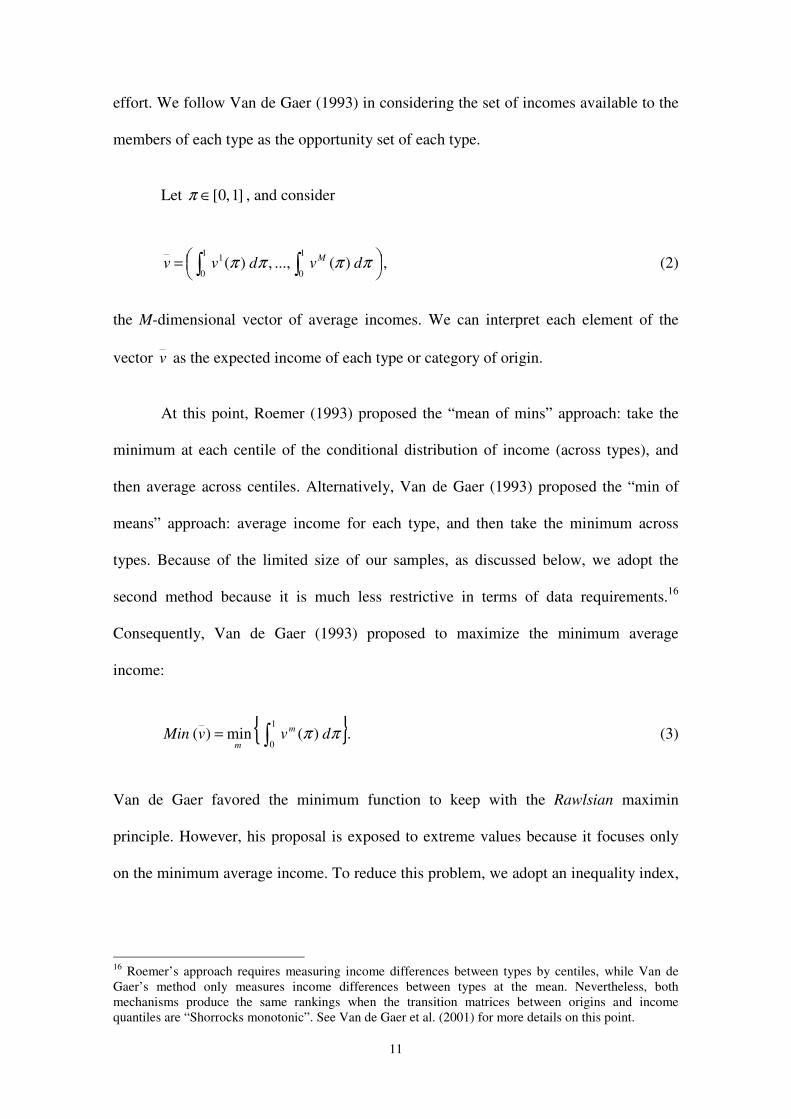
effort. We follow Van de Gaer (1993) in considering the set of incomes available to the

members of each type as the opportunity set of each type.

Let ]1,0[∈π , and consider

= ∫∫ ππππ dvdvv

M)(...,,)(

1

0

1

0

1, (2)

the M-dimensional vector of average incomes. We can interpret each element of the

vector v as the expected income of each type or category of origin.

At this point, Roemer (1993) proposed the “mean of mins” approach: take the

minimum at each centile of the conditional distribution of income (across types), and

then average across centiles. Alternatively, Van de Gaer (1993) proposed the “min of

means” approach: average income for each type, and then take the minimum across

types. Because of the limited size of our samples, as discussed below, we adopt the

second method because it is much less restrictive in terms of data requirements.16

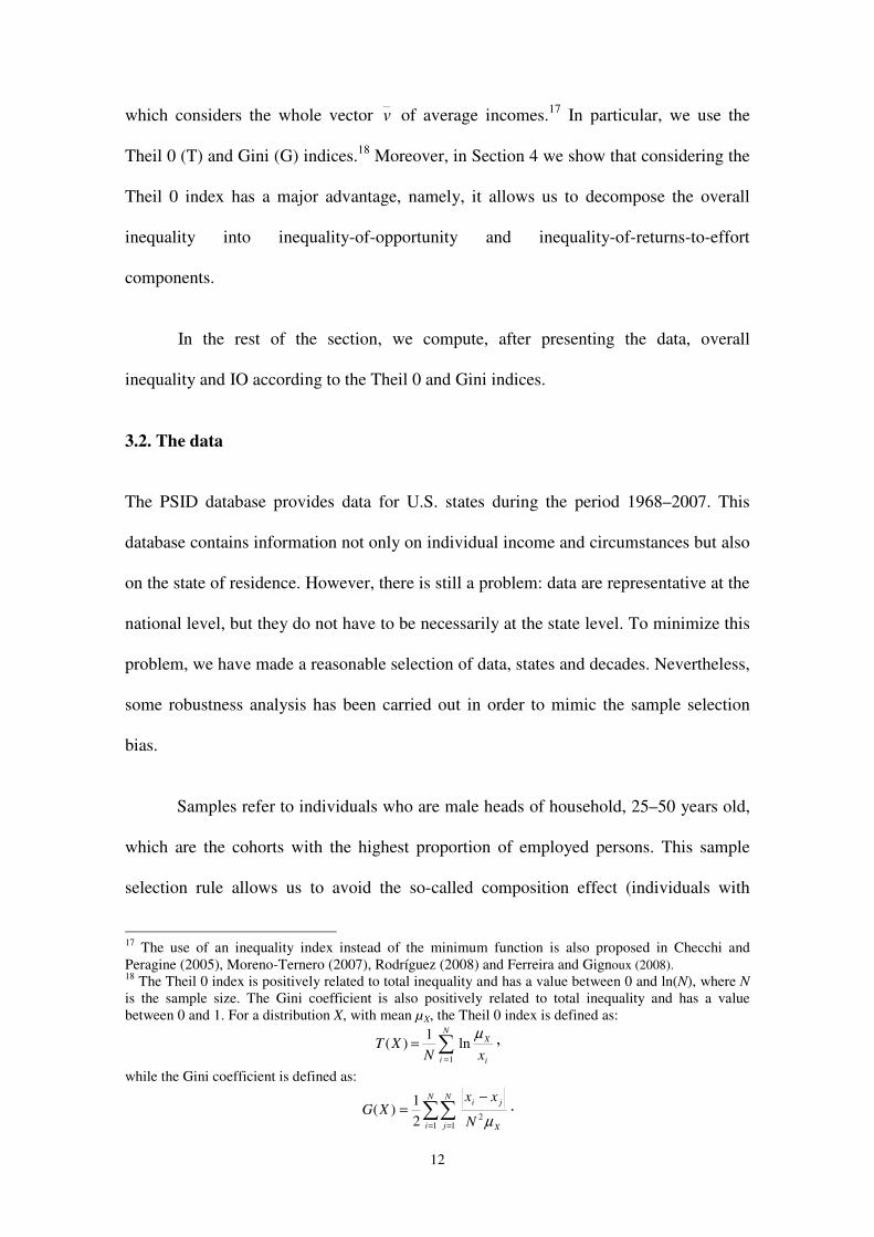
Consequently, Van de Gaer (1993) proposed to maximize the minimum average

income:

{ }ππ dvvMin m

m)(min)(

1

0∫= . (3)

Van de Gaer favored the minimum function to keep with the Rawlsian maximin

principle. However, his proposal is exposed to extreme values because it focuses only

on the minimum average income. To reduce this problem, we adopt an inequality index,

16

Roemer’s approach requires measuring income differences between types by centiles, while Van de

Gaer’s method only measures income differences between types at the mean. Nevertheless, both

mechanisms produce the same rankings when the transition matrices between origins and income

quantiles are “Shorrocks monotonic”. See Van de Gaer et al. (2001) for more details on this point.

12

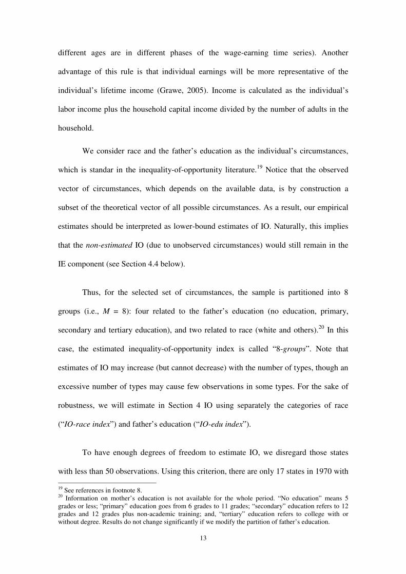
which considers the whole vector v of average incomes.17

In particular, we use the

Theil 0 (T) and Gini (G) indices.18

Moreover, in Section 4 we show that considering the

Theil 0 index has a major advantage, namely, it allows us to decompose the overall

inequality into inequality-of-opportunity and inequality-of-returns-to-effort

components.

In the rest of the section, we compute, after presenting the data, overall

inequality and IO according to the Theil 0 and Gini indices.

3.2. The data

The PSID database provides data for U.S. states during the period 1968–2007. This

database contains information not only on individual income and circumstances but also

on the state of residence. However, there is still a problem: data are representative at the

national level, but they do not have to be necessarily at the state level. To minimize this

problem, we have made a reasonable selection of data, states and decades. Nevertheless,

some robustness analysis has been carried out in order to mimic the sample selection

bias.

Samples refer to individuals who are male heads of household, 25–50 years old,

which are the cohorts with the highest proportion of employed persons. This sample

selection rule allows us to avoid the so-called composition effect (individuals with

17

The use of an inequality index instead of the minimum function is also proposed in Checchi and

Peragine (2005), Moreno-Ternero (2007), Rodríguez (2008) and Ferreira and Gignoux (2008). 18

The Theil 0 index is positively related to total inequality and has a value between 0 and ln(N), where N

is the sample size. The Gini coefficient is also positively related to total inequality and has a value

between 0 and 1. For a distribution X, with mean µX, the Theil 0 index is defined as:

∑=

=N

i i

X

xNXT

1

ln1

)(µ ,

while the Gini coefficient is defined as:

∑∑= =

−=

N

i

N

j X

ji

N

xxXG

1 122

1)(

µ.

13

different ages are in different phases of the wage-earning time series). Another

advantage of this rule is that individual earnings will be more representative of the

individual’s lifetime income (Grawe, 2005). Income is calculated as the individual’s

labor income plus the household capital income divided by the number of adults in the

household.

We consider race and the father’s education as the individual’s circumstances,

which is standar in the inequality-of-opportunity literature.19

Notice that the observed

vector of circumstances, which depends on the available data, is by construction a

subset of the theoretical vector of all possible circumstances. As a result, our empirical

estimates should be interpreted as lower-bound estimates of IO. Naturally, this implies

that the non-estimated IO (due to unobserved circumstances) would still remain in the

IE component (see Section 4.4 below).

Thus, for the selected set of circumstances, the sample is partitioned into 8

groups (i.e., M = 8): four related to the father’s education (no education, primary,

secondary and tertiary education), and two related to race (white and others).20

In this

case, the estimated inequality-of-opportunity index is called “8-groups”. Note that

estimates of IO may increase (but cannot decrease) with the number of types, though an

excessive number of types may cause few observations in some types. For the sake of

robustness, we will estimate in Section 4 IO using separately the categories of race

(“IO-race index”) and father’s education (“IO-edu index”).

To have enough degrees of freedom to estimate IO, we disregard those states

with less than 50 observations. Using this criterion, there are only 17 states in 1970 with

19

See references in footnote 8. 20

Information on mother’s education is not available for the whole period. “No education” means 5

grades or less; “primary” education goes from 6 grades to 11 grades; “secondary” education refers to 12

grades and 12 grades plus non-academic training; and, “tertiary” education refers to college with or

without degree. Results do not change significantly if we modify the partition of father’s education.

14

at least 50 observations. Moreover, there were 2,116 observations for the U.S. as a

whole in 1970, whereas the numbers of observations were 3,091 and 3,843 in 1980 and

1990, respectively. Hence, to assure a large enough sample size for each state, we

disregard the 1970s and focus on the 1980s and 1990s. For these two decades, our final

sample reduces to the following 23 states: Arkansas, California, Florida, Georgia,

Illinois, Indiana, Iowa, Kentucky, Louisiana, Maryland, Massachusetts, Michigan,

Mississippi, Missouri, New Jersey, New York, North Carolina, Ohio, Pennsylvania,

South Carolina, Tennessee, Texas, and Virginia.

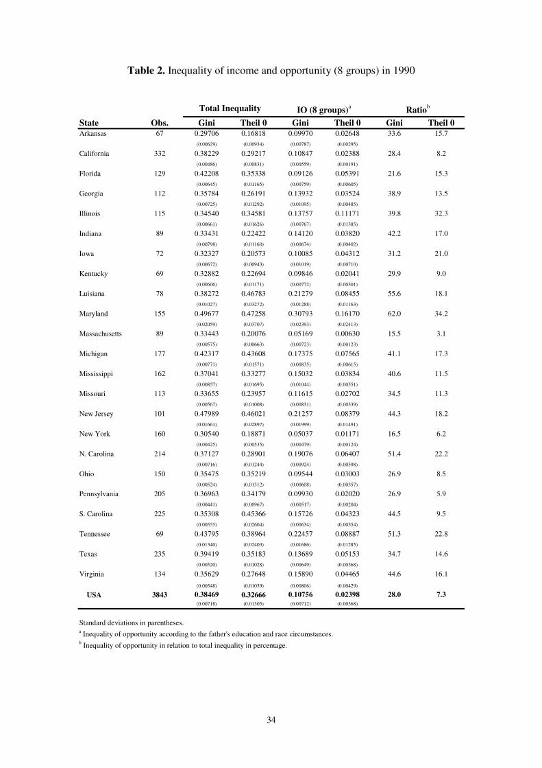
3.3. Inequality of income and opportunity in the U.S. states

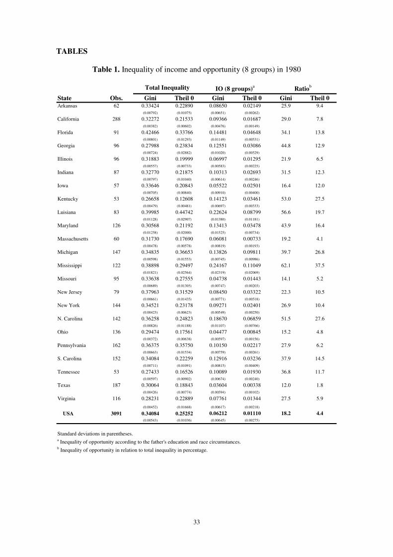
For the 23 selected U.S. states, Tables 1 and 2 show income inequality and IO estimates

for 1980 and 1990, respectively.21

They show results for the Theil 0 and Gini indices

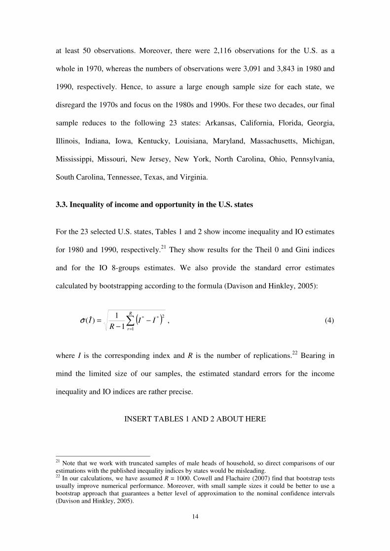
and for the IO 8-groups estimates. We also provide the standard error estimates

calculated by bootstrapping according to the formula (Davison and Hinkley, 2005):

( )∑=

−−

=R

r

IIR

I1

2**

1

1)ˆ(σ̂ , (4)

where I is the corresponding index and R is the number of replications.22

Bearing in

mind the limited size of our samples, the estimated standard errors for the income

inequality and IO indices are rather precise.

INSERT TABLES 1 AND 2 ABOUT HERE

21

Note that we work with truncated samples of male heads of household, so direct comparisons of our

estimations with the published inequality indices by states would be misleading. 22

In our calculations, we have assumed R = 1000. Cowell and Flachaire (2007) find that bootstrap tests

usually improve numerical performance. Moreover, with small sample sizes it could be better to use a

bootstrap approach that guarantees a better level of approximation to the nominal confidence intervals

(Davison and Hinkley, 2005).

15

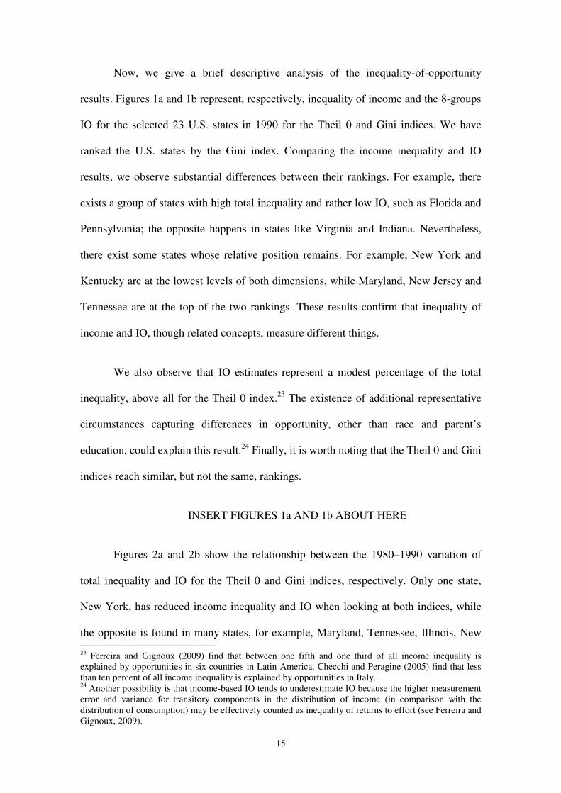
Now, we give a brief descriptive analysis of the inequality-of-opportunity

results. Figures 1a and 1b represent, respectively, inequality of income and the 8-groups

IO for the selected 23 U.S. states in 1990 for the Theil 0 and Gini indices. We have

ranked the U.S. states by the Gini index. Comparing the income inequality and IO

results, we observe substantial differences between their rankings. For example, there

exists a group of states with high total inequality and rather low IO, such as Florida and

Pennsylvania; the opposite happens in states like Virginia and Indiana. Nevertheless,

there exist some states whose relative position remains. For example, New York and

Kentucky are at the lowest levels of both dimensions, while Maryland, New Jersey and

Tennessee are at the top of the two rankings. These results confirm that inequality of

income and IO, though related concepts, measure different things.

We also observe that IO estimates represent a modest percentage of the total

inequality, above all for the Theil 0 index.23

The existence of additional representative

circumstances capturing differences in opportunity, other than race and parent’s

education, could explain this result.24

Finally, it is worth noting that the Theil 0 and Gini

indices reach similar, but not the same, rankings.

INSERT FIGURES 1a AND 1b ABOUT HERE

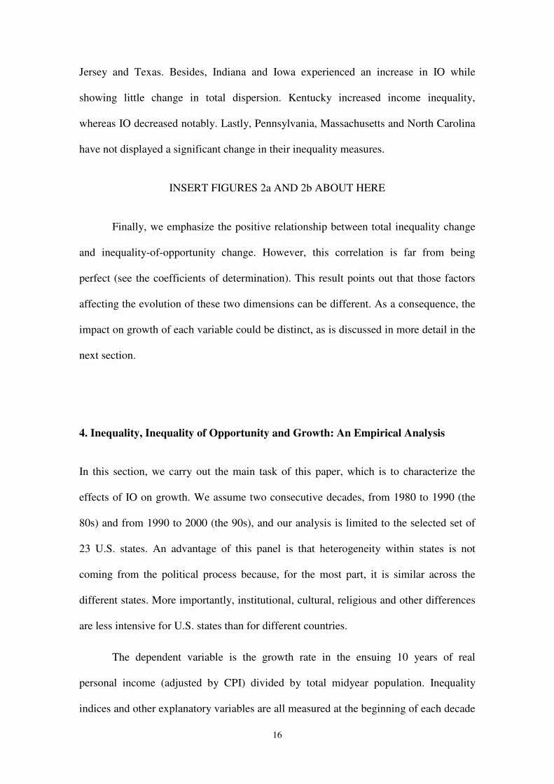
Figures 2a and 2b show the relationship between the 1980–1990 variation of

total inequality and IO for the Theil 0 and Gini indices, respectively. Only one state,

New York, has reduced income inequality and IO when looking at both indices, while

the opposite is found in many states, for example, Maryland, Tennessee, Illinois, New 23

Ferreira and Gignoux (2009) find that between one fifth and one third of all income inequality is

explained by opportunities in six countries in Latin America. Checchi and Peragine (2005) find that less

than ten percent of all income inequality is explained by opportunities in Italy. 24

Another possibility is that income-based IO tends to underestimate IO because the higher measurement

error and variance for transitory components in the distribution of income (in comparison with the

distribution of consumption) may be effectively counted as inequality of returns to effort (see Ferreira and

Gignoux, 2009).

16

Jersey and Texas. Besides, Indiana and Iowa experienced an increase in IO while

showing little change in total dispersion. Kentucky increased income inequality,

whereas IO decreased notably. Lastly, Pennsylvania, Massachusetts and North Carolina

have not displayed a significant change in their inequality measures.

INSERT FIGURES 2a AND 2b ABOUT HERE

Finally, we emphasize the positive relationship between total inequality change

and inequality-of-opportunity change. However, this correlation is far from being

perfect (see the coefficients of determination). This result points out that those factors

affecting the evolution of these two dimensions can be different. As a consequence, the

impact on growth of each variable could be distinct, as is discussed in more detail in the

next section.

4. Inequality, Inequality of Opportunity and Growth: An Empirical Analysis

In this section, we carry out the main task of this paper, which is to characterize the

effects of IO on growth. We assume two consecutive decades, from 1980 to 1990 (the

80s) and from 1990 to 2000 (the 90s), and our analysis is limited to the selected set of

23 U.S. states. An advantage of this panel is that heterogeneity within states is not

coming from the political process because, for the most part, it is similar across the

different states. More importantly, institutional, cultural, religious and other differences

are less intensive for U.S. states than for different countries.

The dependent variable is the growth rate in the ensuing 10 years of real

personal income (adjusted by CPI) divided by total midyear population. Inequality

indices and other explanatory variables are all measured at the beginning of each decade

17

(1980 and 1990). This strategy saves us from endogeneity and measurement errors. In

this manner, we can apply standard pooling regressions techniques, such as in Barro and

Sala-i-Martin (1991), Partridge (1997) and many others.

To measure the relationship between inequality, IO and growth properly, the

model must include additional variables that also affect growth. We use the controls that

were significant in Partridge (1997). In a first and more parsimonious specification -

specification (1) -, we consider a convergence term, time and regional dummies and the

average skills of the labor force. In a second specification - specification (2) -, we also

include variables capturing sectoral composition and past labor growth.25

More specifically, the lagged level of real per capita income is included in the

model to control for conditional convergence across states.26

In addition, we consider a

time dummy for the 80s, and we omit the dummy for the 90s. We also use a standard

and broad classification for regional variables: West, Midwest, South and Northeast.27

The omitted regional dummy is the Northeast region. We consider three categories to

measure the average skills of the labor force: the percentage of the population over 24

years old who have graduated from high school but do not have a four-year college

degree (high school); the percentage who have graduated from a four-year college

(college); and the omitted category, which is the percentage of individuals who have not

graduated from high school.28

To control for the initial economic sectoral mix of each

25

Population and personal income data come from the Regional Economic Accounts of the Bureau of

Economic Analysis (U.S. Department of Commerce, http://www.bea.gov/regional/spi/drill.cfm), while

CPI data come from the U.S. Department of Labor (All Urban Consumers CPI series:

http://www.bls.gov/data/#prices); employment data (total and by type of industry) come from the Current

Employment Statistics of the Bureau of Labor Statistics (U.S. Department of Labor:

http://www.bls.gov/data/#employment). 26

As is the norm in the convergence literature, an implicit assumption is that economic growth is

converging to an equilibrium growth path that is a function of initial conditions (Barro and Sala-i-Martin,

1991) 27

Regional dummies consider those fixed factors that are time invariant and inherent to each area but are

not observed or not included in the model, such as geographical, social or local policy regional aspects or

initial technology efficiency. 28

Historical Census Statistics on Education Attained in the U.S., 1940 to 2000 (U.S. Census Bureau):

18

state, the shares of nonagricultural employment are included for mining, construction,

manufacturing, transportation and public utilities, finance, insurance and real estate,

and government. Traded goods and services are the omitted sector, and thus the

employment share coefficients should be interpreted as being relative to this sector. The

percentage of the population who worked on a farm (farm) is included to account for the

different importance of agriculture across states. Finally, in order to account for the

possibility that growth in the previous decade could, in turn, influence growth in the

following decade and be correlated with past inequality, we include the percentage

change in nonagricultural employment in the preceding decade (e.g., employment

growth in the 80s is used to explain per capita income growth in the 90s).

4.1. Income inequality and growth

The benchmark analysis is based on regressions between growth, lagged income, an

overall inequality index (Theil 0 and Gini) and the set of control variables:

itsititsitsitit XRTIyGY ελδαφβ +++++= −−− '''·· , (5)

where GYit is real per capita income growth in the decade, yit–s is the real per capita

income of state i at the beginning of the decade, Iit–s is the overall inequality index at the

beginning of the decade, Tt is the time dummy corresponding to the 80s, Ri is a set of

regional dummies, Xit–s groups the rest of control variables measured at the beginning of

the decade, and finally εit encompasses effects of a random nature that are not

considered in the model and is assumed to have the standard error component structure.

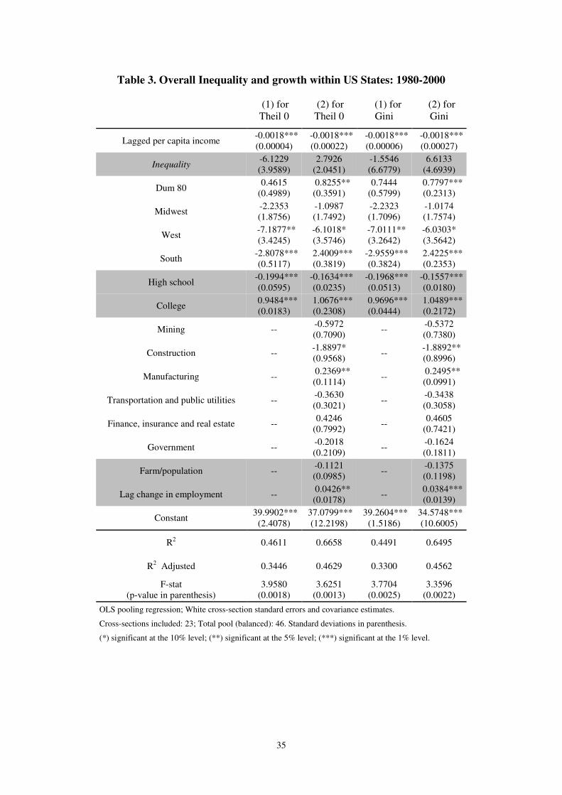
Results for this benchmark setting are shown in Table 3. As in the rest of the paper,

http://www.census.gov/population/www/socdemo/education/introphct41.html.

19

results are based on the standard OLS pooling regression and White cross-sectional

standard errors and covariance matrix.

INSERT TABLE 3 ABOUT HERE

Regardless of the model specification, the results for the control variables are

fairly robust and are in line with the related literature. The negative coefficient for

lagged per capita income reflects conditional convergence, and its magnitude is in

accordance with Barro and Sala-i-Martin (1991). Future economic growth is expected to

be positively correlated with the labor force’s human capital. As is commonly found in

growth models augmented for human capital, the relevant variable of education is

college, which is highly positive and significant with respect to the omitted category

(non-graduated). However, we find that the effect of high school on growth is negative,

but small, with respect to this category. The coefficients on most of the initial industrial

mix variables are negative, though only construction is significant. The exception is

manufacturing, whose coefficient is positive and significant. These findings suggest that

states with greater initial shares in services and traded goods (the omitted category) and

manufacturing have experienced higher economic growth.

The estimates for the farm variable are negative and no significant, while the

coefficient associated with labor growth in the preceding year is positive and

significant, which corroborates the idea that growth in the previous decade influences

growth in the following decade. Regarding the cross-regional dummies, the coefficient

for South is positive and significant for a full-specified model, while that for West is

negative and significant; the coefficient for Midwest is no significant. Finally, the

dummy for the 80s is positive and significant for a full-specified model.

20

At last, regarding the overall inequality indices, we first notice that Partridge

(1997) found a positive relationship between overall inequality and per capita income

growth. However, we find that the initial Theil 0 and Gini coefficients are no

significant.29

Based on this result, a poor conclusion would be that distributive policies

would not affect growth. Next, we test whether this result is due to the non-distinction

between income inequality and IO. As we will see below, controlling by an inequality-

of-opportunity measure changes the policy message dramatically.

4.2. Inequality of opportunity and growth

Now, we introduce IO into the model. In particular, we include the IO term into the

expression (5) to estimate the following model:

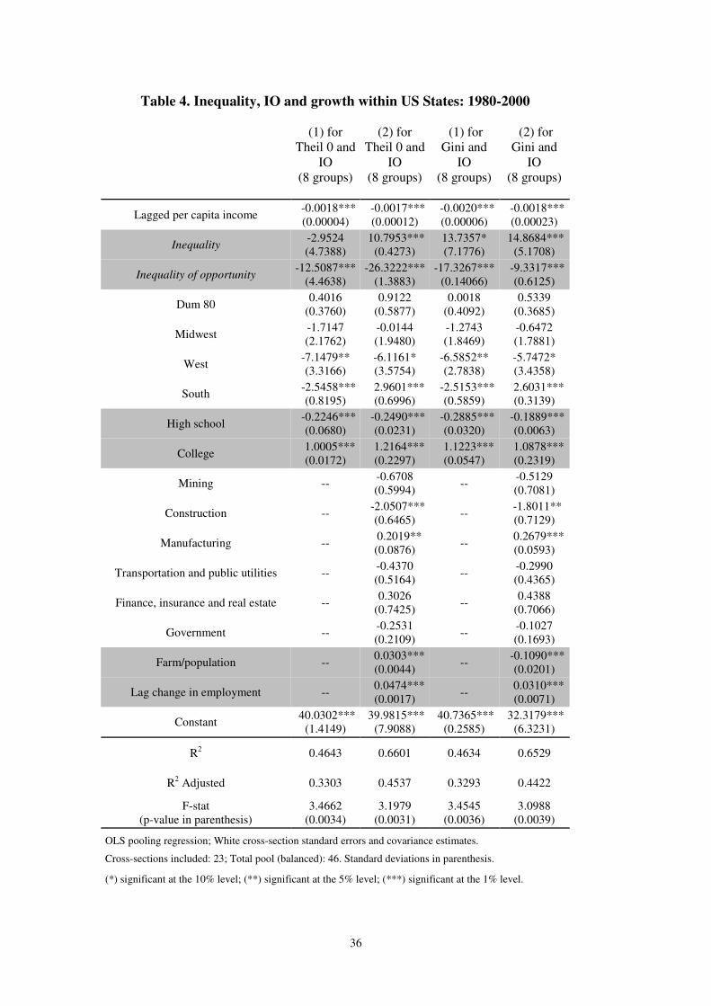
itsititsitsitsitit XRTIOIyGY ελδαφφβ ++++++= −−−− '''··· 21 (6)

where IOit–s is the corresponding inequality-of-opportunity index (8-groups) at the

beginning of the decade.

When including the IO term into the regression, we control for the observed

circumstances, i.e. father’s education and race. As a result, the coefficient of total

inequality would now show the effect of effort and those circumstances that are not

observed. Thus, we would expect that our estimated IO has a negative effect on growth,

and the positive coefficient of total inequality found in Table 3 turns out significant.

These results are confirmed for the Theil 0 and Gini indices, as it is shown in Table 4.

These findings support the thesis that IO and inequality of returns to effort have

opposite effects upon growth. Inequality is good for growth when that comes from

29

Note that our results are not directly comparable with Partridge’s; because we use the PSID database,

our samples refer to male heads of households 25 to 50 years old, and we focus on the 80s and 90s and 23

selected states.

21

differences in the returns to effort, while it is harmful for growth when that comes from

differences in opportunity. Accordingly, policies that equalize opportunity and promote

individual effort will enhance growth.

INSERT TABLE 4 ABOUT HERE

The importance of this result deserves a careful analysis of robustness. The

number and type of circumstances used, the way that income inequality and IO are

combined into the same regression and the number of states considered, are the factors

that we analyze to be more confident in our main result.

4.3. Inequality-of-opportunity estimates: the role of circumstances

Peculiar non-linearity effects on growth of the educational structure might lead to

erroneous conclusions when using father’s education as a circumstance. For instance,

let’s assume that race is not representative because it does not explain much IO and the

explicative variables that measure the average skills of the labor force do not completely

capture the effect of education upon growth. Then, it is possible that the estimated IO

term, which relies on the distribution of people among four educational groups, is

actually capturing part of the effect that education may have on growth. This fact might

cause that the estimated impact of IO would be misleading.30

To check this possibility,

we analyze the explicative power of every circumstance alone.

First, we estimate dispersion in opportunity using separately the circumstance of

race (IO-race) and father’s education (IO-edu). Table 5 shows the indices of IO for our

selected U.S. states in 1980 and 1990. We observe that both circumstances are relevant

for explaining differences in opportunity. For example, when using the Theil 0 index we

30

We are grateful for this suggestion from François Bourguignon.

22

find that IO-race and IO-edu dominate to each other approximately in the same number

of states in 1990. Therefore, the negative impact of IO on growth found in the previous

section (see Table 4) cannot be completely ascribed to father’s education. Even if the

proposed alternative channel through which education may affect growth is true, there is

still room for a negative and significant impact of IO due to race on growth.

INSERT TABLE 5 ABOUT HERE

Table 6 shows the regression results using the IO-race and IO-edu indices under

the full specified model. We first notice that the coefficient for the IO-race measure is

highly significant and negative for both the Theil 0 and the Gini indices. However, the

impact of IO-edu is unclear because its coefficient is negative but non-significant for the

Theil 0 and Gini indices. In respect to the coefficient of total inequality, it is positive

and significant for the 2-groups case (IO-race), and positive but non-significant for the

4-groups case (IO-edu). Consequently, we can be confident in the estimated impact of

IO (8 groups), as long as race has been shown to be the driving force explaining the

negative influence that IO has on growth.

INSERT TABLE 6 ABOUT HERE

4.4. Overall inequality decomposition

Thus far, we have included in the regressions indices of total inequality and IO.

However, the total inequality and IO terms are not independent, which may affect the

estimated coefficient of IO and its significance. In order to avoid this inconvenience, a

further refinement is possible: we can exactly decompose overall inequality into

inequality-of-opportunity and inequality-of-returns-to-effort components. In this

23

manner, the two sources of income differences, circumstances and effort, will be

included separately in the regressions.

As is well known, an inequality index is additively decomposable by population

subgroups if and only if it is a positive multiple of a member of the Generalized Entropy

class (Bourguignon, 1979 and Shorrocks, 1980 and 1984). This means that for every

partition, any member of the Generalized Entropy class can be expressed as the sum of

two terms: a weighted sum of within-group inequalities, plus a between-group

inequality component. Only the Theil 0 index, among the members of the General

Entropy class, uses weights based on the groups’ population shares and has a path-

independent decomposition (Foster and Shneyerov, 2000).31

For both reasons we

consider the Theil 0 index throughout this Section.

Thus, given a particular set of circumstances, consider any partition of income v

into M groups, ( )Mvvv ...,,1= , and v as defined in expression (2), then the Theil 0

index can be decomposed as follows:

∑=

+=M

m

m

m vTpvTvT1

)()()( , (7)

where pm is the frequency of type m in the population. The first term, )(vT , is a

between-group index, which captures the income inequality due to different

circumstances. As it was done in Section 3, this component is calculated by applying

the Theil 0 index to an income vector in which each individual in a given group receives

the corresponding group’s mean income. Thus, this component is, by construction, an

31 The rest members of the General Entropy class use weights based not only on the groups’ population

shares but also on the groups’ income shares. In this manner, these indices give more importance to rich

people.

24

inequality-of-opportunity index. As said above, its accuracy is conditioned by the set of

circumstances being selected, which, in practice, depends on the available data. The

second component is a within-group term, which captures the income inequality within

each type m, weighted by the demographic importance of the corresponding type.

Because income is a function of effort and circumstances, the within-group component

then can be considered as an inequality-of-returns-to-effort index (the IE variable).

Unfortunately, the estimated IE and IO terms will not be completely orthogonal because

the non-estimated IO (due to unobserved circumstances) would still remain in the IE

component.32

After decomposing total inequality into inequality-of-opportunity and inequality-

of-returns-to-effort components, we estimate the following model:

itsititsitsitsitit XRTIOIEyGY ελδαφφβ ++++++= −−−− '''··· 21 . (8)

Table 7 shows the results for this model, using the IO (8 groups), IO-race and IO-edu

estimates. The IE coefficient is positive and significant, while the IO coefficient is

negative and significant for the IO (8 groups) and IO-race estimates. For the IO-edu

index, the coefficients for the IE and IO variables are positive and negative,

respectively, but they are not significant. These results are consistent with previous

findings. In particular, the two components of total inequality, IO and IE, have

significant but opposite effects upon growth. Moreover, race is more important than

father’s education in explaining the negative influence of IO on growth.

32

The Gini index generally fails to decompose additively into between- and within-group components.

Thus, the Gini decomposition is (see, among others, Lambert and Aronson, 1993):

RvGqpvGvGM

m

m

mm ++= ∑=1

)()()( ,

where qm is the income share for type m. The first term is the between-groups Gini coefficient, the second

term is the within-group component, and R is a residual that is zero only in the case that group income

ranges do not overlap, which does not occur in our case.

25

INSERT TABLE 7 ABOUT HERE

4.5. States

Now, we change the states considered in the regressions. Because of the limited size of

our samples, we eliminate those states with fewer observations in 1990.33

Using the

specification in (8), we show in Table 8 the IO and IE coefficients when reducing

recursively the number of states in the regression. Thus, the first line shows the results

when using all 23 states; the second line shows the results when Arkansas, which is the

state with lowest number of observations in 1990, is excluded; in the next row, we

exclude Arkansas and Tennessee, which is the next state with lowest number of

observations; and so on and so forth for the next rows until we keep with 10 states (20

observations).34

Results confirm the positive and significant coefficient for IE and the

negative and significant coefficient for IO. Reducing the number of states, therefore,

neither affects our main result.

INSERT TABLE 8 ABOUT HERE

5. Concluding Remarks

Models exploring the incidence of income inequality upon economic growth do not

reach a clear-cut conclusion. We postulate in this paper that one possible reason for this

inconclusiveness is that income inequality indices are indeed measuring at least two

different sorts of inequality: inequality of opportunity and inequality of effort. Though

33

Similar results are obtained if we eliminate those states with fewer observations in 1980. 34

We are aware of the few degrees of freedom that we have when reducing the number of states, but we

now care only for the robustness of our results.

26

this distinction has already been emphasized in the inequality-of-opportunity literature,

it has not yet been considered in the growth literature.

Using depurated data of the PSID database for 23 U.S. states in 1980 and 1990,

we followed Van de Gaer’s approach to compute inequality-of-opportunity and

inequality-of-returs-to-effort indices. We ran standard OLS pooling regressions, finding

robust support for a negative relationship between inequality of opportunity and growth

and a positive relationship for the other sort of inequality. Hence, these two types of

inequalities are affecting growth through opposite channels. On one hand, inequality of

effort increases growth because it may encourage people to invest in education and to

exert effort. On the other hand, inequality of opportunity decreases growth because it

may not favor human capital accumulation of the more talented individuals. In fact, Van

de Gaer et al. (2001) have pointed out that inequality of opportunity reduces the role

that talent plays in competing for a position by worsening intergenerational mobility.

Making a distinction between inequality of income and inequality of opportunity can

throw some light upon several intriguing empirical facts in the growth literature. Two

examples are pointed out.

Barro (2000) shows a positive relationship between growth and inequality within

most developed countries, while this relationship is negative when looking at the

poorest countries. He proposes, as a tentative explanation, the different role of capital

markets. In particular, he considers that problems of information (moral-hazard and

repayment enforcement problems) are larger in poor countries because they have less-

developed credit markets. However, he does not find empirical evidence for this

different role of capital markets. An alternative explanation that would arise from the

present paper is that differences in opportunity are more important within less-

developed countries. At this respect, some evidence is found in the inequality-of-

27

opportunity literature as in Ferreira and Gignoux (2009), Checchi and Peragine (2005),

Rodríguez (2008) and Cogneau and Mesplé-Somps (2009).

Secondly, some empirical studies have found that the effect of income inequality

on growth is sensitive to the inclusion of some variables like regional dummy variables

(Birdall et al., 1995). However, the relationship between initial land inequality and

growth is negative and robust to the introduction of regional dummies and other

explicative variables (Deininger and Squire, 1998). Our proposal offers an easy

explanation for this empirical fact. Income inequality comes not only from unequal

opportunities but also from different levels of effort. As a result, the effect of income

inequality upon growth can have a different sign depending on the kind of controls that

are introduced in the regressions. However, initial land inequality comes

unambiguously from unequal opportunities (i.e., the socioeconomic conditions of

parents) and has a clear-cut negative effect upon growth.

Further research concerning these issues is clearly needed. However, we believe

that a complete understanding of the relationship between inequality and growth

requires more effort in constructing appropriated databases that properly represent

social origins.

28

REFERENCES

Aghion, P. and Bolton P. (1997), “A trickle-down theory of growth and development

with debt overhang”, Review of Economic Studies, 64, 151-162.

Aghion, P. Caroli, E. and García-Peñalosa, C. (1999), “Inequality and economic growth:

the perspective of the new growth theories”, Journal of Economic Literature, 37,

1615-1660.

Alesina, A. and Rodrik, D. (1994), “Distributive politics and economic growth”,

Quaterly Journal of Economics, 109, 465-490.

Alesina, A. and Perotti, R. (1994), “The political economy of growth: a critical survey

of the recent literature”, The World Bank Economic Review, 8, 350-371.

Alesina, A. and Perotti, R. (1996), “Income distribution, political instability and

investment”, European Economic Review, 40, 1203-1228.

Alesina, A., Ozler, S., Roubini, N. and Swagel, P. (1996), “Political instability and

economic growth”, Journal of Economic Growth, 1, 189-211.

Arrow, K., Bowles, S. and Durlauf, S. (2000), Meritocracy and economic inequality.

Princeton University Press.

Banerjee, A. and Newman, A.F. (1991), “Risk-bearing and the theory of income

distribution”, Review of Economic Studies, 58, 211-235.

Banerjee, A. and Duflo, E. (2003), “Inequality and growth: what can the data say?”,

Journal of Economic Growth, 8, 267-299.

Barro, R. J. (2000), “Inequality and growth in a panel of countries”, Journal of

Economic Growth, 5, 5-32.

Barro, R. J. and Sala-i-Martin, X. (1991), “Convergence across states and regions”,

Brookings Papers on Economic Activity, 1, 107-182.

Bertola, G., Foellmi, R. and Zweimüller, J. (2005), Income distribution in

macroeconomic models. Princeton: Princeton University Press.

Betts, J. and Roemer, J. E. (2007), “Equalizing opportunity for racial and

socioeconomic groups in the United States through educational finance reform”,

in Schools and the Equal Opportunity Problem, P. Peterson (ed.), Cambridge,

M.A.: The MIT Press.

Birdsall, N., Ross, D. and Sabot, R. (1995), “Inequality and growth reconsidered:

lessons from East Asia”, World Bank Economic Review, 9, 477-508.

Bourguignon, F. (1979), “Decomposable income inequality measures”, Econometrica,

47, 901-920.

Bourguignon, F. (1981), “Pareto-superiority of unegalitarian equilibria in Stiglitz' model

of wealth distribution with convex savings function”, Econometrica, 49, 1469-

1475.

Bourguignon, F. (1996), “Equity and economic growth: permanent questions and

changing answers?”, Working Paper 96-15, DELTA Paris.

Bourguignon, F., Ferreira, F. and Menéndez, M. (2007), “Inequality of opportunity in

Brazil”, Review of Income and Wealth, 53, 585-618.

Bourguignon, F., Ferreira, F. and Walton, M. (2007), “Equity, efficiency and inequality

traps: a research agenda”, Journal of Economic Inequality, 5, 235-256.

Checchi, D. and Peragine, V. (2005), “Regional Disparities and inequality of

opportunity: the case of Italy”, IZA Discussion Paper 1874/2005.

Chiu, W. H. (1998), “Income inequality, human capital accumulation and economic

performance”, Economic Journal, 108, 44-59.

29

Clarke, G.R.C. (1995), “More evidence on income distribution and growth”, Journal of

Development Economics, 47, 403-427.

Cogneau, D. and Mesplé-Somps, S. (2009), “Inequality of Opportunity for Income in

Five Countries of Africa”, Research on Economic Inequality, 16, 99-128.

Cowell, F. A. and E. Flachaire (2007): “Income Distribution and Inequality

Measurement: The Problem of Extreme Values", Journal of Econometrics, 141,

1044-1072.

Dahan, M. and Tsiddon, D. (1998), “Demographic transition, income distribution and

economic growth”, Journal of Economic Growth, 3, 29-52.

Dasgupta, P. and Ray, D. (1987), “Inequality as a Determinant of Malnutrition and

Unemployment Policy”, Economic Journal, 97, 177-188.

Davison, A. C. and D. V. Hinkley (2005), Bootstrap methods and their application.

Cambridge University Press, New York.

Deininger, K. and Squire, L. (1996), “A new data set measuring income inequality”, World

Bank Economic Review, 10, 565-591.

Deininger, K. and Squire, L. (1998), “New ways of looking at old issues: inequality and

growth”, Journal of Development Economics, 57, 259-287.

Ehrhart, C. (2009), “The effects of inequality on growth: a survey of the theoretical and

empirical literature”, ECINEQ WP 2009-107.

Falkinger, J. and Zweimüller, J. (1997), “The impact of income inequality on product

diversity and economic growth”, Metroeconomica, 48, 211-237.

Ferreira, F. and Gignoux, J. (2008), “The measurement of inequality of opportunity:

theory and an application to Latin America”, World Bank Policy Research

Working Paper #4659.

Fleurbaey, M. (1995), “Equal opportunity or equal social outcome”, Economics and

Philosophy, 11, 25-56.

Fleurbaey, M. (2008), Fairness, responsibility, and welfare. Oxford: Oxford University

Press.

Fleurbaey M. and F. Maniquet (2007), “Compensation and responsibility”, in The

Handbook for Social Choice and Welfare, Arrow, K., Sen, A. and Suzumura, K.

(eds.), Amsterdan: North Holland.

Forbes, K. (2000), “A reassessment of the relationship between inequality and growth”,

American Economic Review, 90, 869-887.

Foster, J. and Shneyerov, A. (2000), “Path independent inequality measures”, Journal of

Economic Theory, 91, 199-222.

Galenson, W. and Leibenstein, H. (1955), “Investment criteria, productivity and economic

development”, Quaterly Journal of Economics, 69, 343-370.

Galor, O. and Zeira, J. (1993), “Income distribution and macroeconomics”, Review of

Economic Studies, 60, 35-52.

Galor, O. and Zang, H. (1997), “Fertility, income distribution and economic growth:

theory and cross-country race obviousness”, Japan and the world economy, 9, 197-

229.

Grawe, N. (2005), “Lifecycle bias in estimates of intergenerational earnings

persistence”, Labour Economics, 13, 551-570.

Gupta, D. K. (1990), The economics of political violence. The effect of political instability

on economic growth. New York: Praeger Publishers.

Keefer, P. and Knack, S. (2002), “Polarization, politics and property rights: links between

inequality and growth”, Public Choice, 111, 127-154.

30

Khoo, L. and Dennis, B. (1999), “Income inequality, fertility choice, and economic

growth: theory and evidence”, Harvard Institute for International Development

(HIID), Development Discussion Paper 687.

Knowles, S. (2001), “Inequality and economic growth: the empirical relationship

reconsidered in the light of comparable data”. Discussion Paper 105, Department of

Economics, University of Otago (Dunedin), New Zealand.

Kremer, M. and Chen, D. (2002), ”Income distribution dynamics with endogenous

fertility”, Journal of Economic Growth, 7, 227-258.

Kuznets, S. (1955), “Economic growth and income inequality”, American Economic

Review, 45, 1-28.

Lambert, P. J. and Aronson, J. R. (1993), “Inequality decomposition analysis and the

Gini coefficient revisited”, Economic Journal, 103, 1221-1227.

Lefranc, A., Pistolesi, N. and Trannoy A. (2008), “Inequality of opportunities vs.

inequality of outcomes: Are Western societies all alike?”, Review of Income and

Wealth, 54, 513-546.

Lefranc, A., Pistolesi, N. and Trannoy A. (forthcoming), “Equality of opportunity:

Definitions and testable conditions, with an application to income in France”,

Journal of Public Economics.

Loury, G. C. (1981), “Intergenerational transfers and the distribution of earnings”,

Econometrica, 49, 843-867.

Lucas, J. R. (1995), Responsibility. Oxford: Clarendon Press.

Mani, A. (2001), “Income distribution and the demand constraint”, Journal of Economic

Growth, 6, 107-133.

Mason, A. (1988), “Savings, economic growth and demographic change”, Population and

Development Review, 14, 113-144.

Marshall, A. (1988), “Income distribution, the domestic market and growth in Argentina”,

Labour and Society, 13 (1), 79-103.

Milanovic, B. (1994), “Determinants of cross-country income inequality : an augmented

Kuznets hypothesis”, Policy Research Working Paper Series, 1246, The World

Bank.

Mirrless, J. (1971), “An exploration in the theory of optimum income taxation”, Review of

Economic Studies, 38, 175-208.

Morand, O. F. (1998), “Endogenous fertility, income distribution, and growth”, Journal

of Economic Growth, 4, 331-349.

Moreno-Ternero, J. D. (2007), “On the design of equal-opportunity policies”,

Investigaciones Económicas, 31, 351-374.

Murphy, K. M., Schleifer, A. and Vishny, R. (1989), “Income distribution, market size,

and industrialization”, Quaterly Journal of Economics, 104, 537-564.

Ooghe, E., Schokkaert E. and D. Van de gaer (2007), “Equality of opportunity versus

equality of opportunity sets”, Social Choice and Welfare, 28, 209-230.

Partridge, M. D. (1997), “Is Inequality Harmful for Growth? Comment”, American

Economic Review, 87, 5, 1019-1032.

Peragine, V. (2002), “Opportunity egalitarianism and income inequality”, Mathematical

Social Sciences, 44, 45-60.

Peragine, V. (2004), “Ranking of income distributions according to equality of

opportunity”, Journal of Income Inequality, 2, 11-30.

Perottti, R. (1992), “Income distribution, politics and growth”, American Economic Review

82, 311-316.

Perottti, R. (1996), “Growth, income distribution and democracy: what the data say”,

Journal of Economic Growth, 1, 149-187.

31

Persson, T. and Tabellini, G. (1994), “Is inequality harmful for growth?: theory and

evidence”, American Economic Review, 84, 600-621.

Piketty, T. (1997), “The dynamics of the wealth distribution and the interest rate with

credit rationing”, Review of Economic Studies, 64, 173-189.

Rebelo, S. (1991), “Long-run policy analysis and long-run growth”, Quaterly Journal of

Economics, 107, 255-284.

Roemer, J. E. (1993), “A pragmatic approach to responsibility for the egalitarian

planner”, Philosophy & Public Affairs, 10, pp. 146-166.

Roemer, J.E. (1996), Theories of Distributive Justice. Harvard University Press,

Cambridge, M.A.

Roemer, J.E. (1998), Equality of Opportunity. Harvard University Press, Cambridge,

M.A.

Roemer, J.E. (2002), “Equality of opportunity: a progress report”, Social Choice and

Welfare, 19, 455-471.

Roemer, J.E., Aaberge, R., Colombino, U., Fritzell, J., Jenkins, S., Marx, I., Page, M.,

Pommer, E., Ruiz-Castillo, J., San Segundo, M. J., Tranaes, T., Wagner, G. and

Zubiri, I. (2003), “To what extent do fiscal regimes equalize opportunities for

income acquisition among citizens?”, Journal of Public Economics, 87, 539-565.

Rodríguez, J. G. (2008), “Partial equality-of-opportunity orderings”, Social Choice and

Welfare, 31, 435-456.

Ruiz-Castillo, J. (2003), “The measurement of the inequality of opportunities”,

Research on Economic Inequality, 9, 1-34.

Shorrocks, A. F. (1980), “The class of additively decomposable inequality measures”,

Econometrica, 48, 613-625.

Shorrocks, A. F. (1984), “Inequality Decomposition by population subgroups”,

Econometrica, 52, 1369-1388.

Stiglitz, J.E. (1969), “The distribution of income and wealth among individuals”,

Econometrica, 37, 382-397.

Svensson, J. (1998), “Investment, property rights and political instability: theory and

evidence”, European Economic Review, 42, 1317-1341.

Székeli, M. (2003), “The 1990s in Latin America: Another decade of persistent

inequality, but with somewhat lower poverty”, Journal of Applied Economics, VI,

317-339.

Todaro, M.P. (1994), Economic development. New York, London: Longman.

Tornell, A. and Velasco, A. (1992), “The tragedy of the commons and economic

growth: why does capital flows from poor to rich countries?”, Journal of Political

Economy, 100, 1208-1231.

Van de Gaer, D. (1993), “Equality of opportunity and investment in human capital”,

Catholic University of Leuven, Faculty of Economics, no. 92.

Van de Gaer D., E. Schokkaert and M. Martinez, (2001), “Three meanings of

intergenerational mobility”, Economica, 68, 519-538.

U.S. Census Bureau, Department of Commerce. Decennial census of population:

Characteristics of the population. Washington, DC: U.S. Government Printing

Office, various years.

U.S. Bureau of Economic Analysis, Department of Commerce. Regional Economic

Accounts. Washington, DC: U.S. Government Printing Office, various years.

U.S. Department of Agriculture. Agricultural statistics. Washington, DC: U.S.

Government Printing Office, various years.

32

U.S. Department of Labour. Employment, hours and earnings. Washington, DC: U.S.

Government Printing Office, various issues.

U.S. Department of Labour. Geographic profile of employment and unemployment.

Washington, DC: U.S. Government Printing Office, various years.

World Bank (2006), World development report 2006: equity and development,

Washington, DC: The World Bank and Oxford University Press.

Zweimüller, J. (2000), “Schumpeterian entrepreneurs meet Engel´s law: the impact of

inequality on innovation-driven growth”, Journal of Economic Growth, 5, 185-

206.

Zou, H. and Li, H. (1998), “Income inequality is not harmful for growth: theory and

evidence”, Journal of Development Economics, 2, 318-334.

33

TABLES

Table 1. Inequality of income and opportunity (8 groups) in 1980

State Obs. Gini Theil 0 Gini Theil 0 Gini Theil 0

Arkansas 62 0.33424 0.22890 0.08650 0.02149 25.9 9.4

(0.00792) (0.01075) (0.00651) (0.00262)

California 288 0.32272 0.21533 0.09366 0.01687 29.0 7.8

(0.00382) (0.00602) (0.00476) (0.00149)

Florida 91 0.42466 0.33766 0.14481 0.04648 34.1 13.8

(0.00801) (0.01293) (0.01149) (0.00531)

Georgia 96 0.27988 0.23834 0.12551 0.03086 44.8 12.9

(0.00724) (0.02882) (0.01020) (0.00529)

Illinois 96 0.31883 0.19999 0.06997 0.01295 21.9 6.5

(0.00557) (0.00733) (0.00583) (0.00225)

Indiana 87 0.32770 0.21875 0.10313 0.02693 31.5 12.3

(0.00797) (0.01040) (0.00614) (0.00246)

Iowa 57 0.33646 0.20843 0.05522 0.02501 16.4 12.0

(0.00705) (0.00840) (0.00910) (0.00400)

Kentucky 53 0.26658 0.12608 0.14123 0.03461 53.0 27.5

(0.00479) (0.00481) (0.00697) (0.00333)

Luisiana 83 0.39985 0.44742 0.22624 0.08799 56.6 19.7

(0.01128) (0.02907) (0.01380) (0.01181)

Maryland 126 0.30568 0.21192 0.13413 0.03478 43.9 16.4

(0.01258) (0.02000) (0.01525) (0.00734)

Massachusetts 60 0.31730 0.17690 0.06081 0.00733 19.2 4.1

(0.00478) (0.00578) (0.00819) (0.00193)

Michigan 147 0.34835 0.36653 0.13826 0.09811 39.7 26.8

(0.00598) (0.01553) (0.00745) (0.00986)

Mississippi 122 0.38898 0.29497 0.24167 0.11049 62.1 37.5

(0.01821) (0.02564) (0.02319) (0.02069)

Missouri 95 0.33638 0.27555 0.04738 0.01443 14.1 5.2

(0.00689) (0.01305) (0.00747) (0.00203)

New Jersey 79 0.37963 0.31529 0.08450 0.03322 22.3 10.5

(0.00661) (0.01435) (0.00771) (0.00518)

New York 144 0.34521 0.23178 0.09271 0.02401 26.9 10.4

(0.00423) (0.00623) (0.00549) (0.00250)

N. Carolina 142 0.36258 0.24823 0.18670 0.06859 51.5 27.6

(0.00826) (0.01188) (0.01107) (0.00766)

Ohio 136 0.29474 0.17561 0.04477 0.00845 15.2 4.8

(0.00372) (0.00638) (0.00597) (0.00156)

Pennsylvania 162 0.36375 0.35750 0.10150 0.02217 27.9 6.2

(0.00663) (0.01534) (0.00759) (0.00261)

S. Carolina 152 0.34084 0.22259 0.12916 0.03236 37.9 14.5

(0.00711) (0.01091) (0.00815) (0.00409)

Tennessee 53 0.27433 0.16526 0.10089 0.01930 36.8 11.7

(0.00597) (0.00902) (0.00674) (0.00240)

Texas 187 0.30064 0.18843 0.03604 0.00338 12.0 1.8

(0.00426) (0.00774) (0.00594) (0.00102)

Virginia 116 0.28231 0.22889 0.07761 0.01344 27.5 5.9

(0.00452) (0.01668) (0.00617) (0.00218)

USA 3091 0.34084 0.25252 0.06212 0.01110 18.2 4.4

(0.00543) (0.01036) (0.00645) (0.00275)

Standard deviations in parentheses.a Inequality of opportunity according to the father's education and race circumstances.

b Inequality of opportunity in relation to total inequality in percentage.

Total Inequality IO (8 groups)a

Ratiob

34

Table 2. Inequality of income and opportunity (8 groups) in 1990

State Obs. Gini Theil 0 Gini Theil 0 Gini Theil 0

Arkansas 67 0.29706 0.16818 0.09970 0.02648 33.6 15.7

(0.00629) (0.00934) (0.00787) (0.00295)

California 332 0.38229 0.29217 0.10847 0.02388 28.4 8.2

(0.00486) (0.00831) (0.00559) (0.00191)

Florida 129 0.42208 0.35338 0.09126 0.05391 21.6 15.3

(0.00645) (0.01165) (0.00759) (0.00605)

Georgia 112 0.35784 0.26191 0.13932 0.03524 38.9 13.5

(0.00725) (0.01292) (0.01095) (0.00485)

Illinois 115 0.34540 0.34581 0.13757 0.11171 39.8 32.3

(0.00661) (0.01626) (0.00767) (0.01385)

Indiana 89 0.33431 0.22422 0.14120 0.03820 42.2 17.0

(0.00798) (0.01160) (0.00674) (0.00402)

Iowa 72 0.32327 0.20573 0.10085 0.04312 31.2 21.0

(0.00672) (0.00943) (0.01019) (0.00710)

Kentucky 69 0.32882 0.22694 0.09846 0.02041 29.9 9.0

(0.00606) (0.01171) (0.00772) (0.00301)

Luisiana 78 0.38272 0.46783 0.21279 0.08455 55.6 18.1

(0.01027) (0.03272) (0.01288) (0.01163)

Maryland 155 0.49677 0.47258 0.30793 0.16170 62.0 34.2

(0.02059) (0.03707) (0.02393) (0.02413)

Massachusetts 89 0.33443 0.20076 0.05169 0.00630 15.5 3.1

(0.00575) (0.00663) (0.00723) (0.00123)

Michigan 177 0.42317 0.43608 0.17375 0.07565 41.1 17.3

(0.00771) (0.01571) (0.00835) (0.00615)

Mississippi 162 0.37041 0.33277 0.15032 0.03834 40.6 11.5

(0.00857) (0.01695) (0.01044) (0.00551)

Missouri 113 0.33655 0.23957 0.11615 0.02702 34.5 11.3

(0.00567) (0.01008) (0.00831) (0.00339)

New Jersey 101 0.47989 0.46021 0.21257 0.08379 44.3 18.2

(0.01661) (0.02897) (0.01999) (0.01491)

New York 160 0.30540 0.18871 0.05037 0.01171 16.5 6.2

(0.00425) (0.00535) (0.00479) (0.00124)

N. Carolina 214 0.37127 0.28901 0.19076 0.06407 51.4 22.2

(0.00716) (0.01244) (0.00924) (0.00598)

Ohio 150 0.35475 0.35219 0.09544 0.03003 26.9 8.5

(0.00524) (0.01312) (0.00608) (0.00357)

Pennsylvania 205 0.36963 0.34179 0.09930 0.02020 26.9 5.9

(0.00441) (0.00967) (0.00517) (0.00204)

S. Carolina 225 0.35308 0.45366 0.15726 0.04323 44.5 9.5

(0.00555) (0.02604) (0.00634) (0.00354)

Tennessee 69 0.43795 0.38964 0.22457 0.08887 51.3 22.8

(0.01340) (0.02403) (0.01686) (0.01285)

Texas 235 0.39419 0.35183 0.13689 0.05153 34.7 14.6

(0.00520) (0.01028) (0.00649) (0.00368)

Virginia 134 0.35629 0.27648 0.15890 0.04465 44.6 16.1

(0.00548) (0.01039) (0.00806) (0.00429)

USA 3843 0.38469 0.32666 0.10756 0.02398 28.0 7.3

(0.00718) (0.01305) (0.00712) (0.00368)

Standard deviations in parentheses.a Inequality of opportunity according to the father's education and race circumstances.

b Inequality of opportunity in relation to total inequality in percentage.

Total Inequality IO (8 groups)a

Ratiob

35

Table 3. Overall Inequality and growth within US States: 1980-2000

(1) for

Theil 0

(2) for

Theil 0

(1) for

Gini

(2) for

Gini

Lagged per capita income -0.0018***

(0.00004)

-0.0018***

(0.00022)

-0.0018***

(0.00006)

-0.0018***

(0.00027)

Inequality -6.1229

(3.9589)

2.7926

(2.0451)

-1.5546

(6.6779)

6.6133

(4.6939)

Dum 80 0.4615

(0.4989)

0.8255**

(0.3591)

0.7444

(0.5799)

0.7797***

(0.2313)

Midwest -2.2353

(1.8756)

-1.0987

(1.7492)

-2.2323

(1.7096)

-1.0174

(1.7574)

West -7.1877**

(3.4245)

-6.1018*

(3.5746)

-7.0111**

(3.2642)

-6.0303*

(3.5642)

South -2.8078***

(0.5117)

2.4009***

(0.3819)

-2.9559***

(0.3824)

2.4225***

(0.2353)

High school -0.1994***

(0.0595)

-0.1634***

(0.0235)

-0.1968***

(0.0513)

-0.1557***

(0.0180)

College 0.9484***

(0.0183)

1.0676***

(0.2308)

0.9696***

(0.0444)

1.0489***

(0.2172)

Mining -- -0.5972

(0.7090) --

-0.5372

(0.7380)

Construction -- -1.8897*

(0.9568) --

-1.8892**

(0.8996)

Manufacturing -- 0.2369**

(0.1114) --

0.2495**

(0.0991)

Transportation and public utilities -- -0.3630

(0.3021) --

-0.3438

(0.3058)

Finance, insurance and real estate -- 0.4246

(0.7992) --

0.4605

(0.7421)

Government -- -0.2018

(0.2109) --

-0.1624

(0.1811)

Farm/population -- -0.1121

(0.0985) --

-0.1375

(0.1198)

Lag change in employment -- 0.0426**

(0.0178) --

0.0384***

(0.0139)

Constant 39.9902***

(2.4078)

37.0799***

(12.2198)

39.2604***

(1.5186)

34.5748***

(10.6005)

R2 0.4611 0.6658 0.4491 0.6495

R2 Adjusted 0.3446 0.4629 0.3300 0.4562

F-stat

(p-value in parenthesis)

3.9580

(0.0018)

3.6251

(0.0013)

3.7704

(0.0025)

3.3596

(0.0022)

OLS pooling regression; White cross-section standard errors and covariance estimates.

Cross-sections included: 23; Total pool (balanced): 46. Standard deviations in parenthesis.

(*) significant at the 10% level; (**) significant at the 5% level; (***) significant at the 1% level.

36

Table 4. Inequality, IO and growth within US States: 1980-2000

(1) for

Theil 0 and

IO

(8 groups)

(2) for

Theil 0 and

IO

(8 groups)

(1) for

Gini and

IO

(8 groups)

(2) for

Gini and

IO

(8 groups)

Lagged per capita income -0.0018***

(0.00004)

-0.0017***

(0.00012)

-0.0020***

(0.00006)

-0.0018***

(0.00023)

Inequality -2.9524

(4.7388)

10.7953***

(0.4273)

13.7357*

(7.1776)

14.8684***

(5.1708)

Inequality of opportunity -12.5087***

(4.4638)

-26.3222***

(1.3883)

-17.3267***

(0.14066)

-9.3317***

(0.6125)

Dum 80 0.4016

(0.3760)

0.9122

(0.5877)

0.0018

(0.4092)

0.5339

(0.3685)

Midwest -1.7147

(2.1762)

-0.0144

(1.9480)

-1.2743

(1.8469)

-0.6472

(1.7881)

West -7.1479**

(3.3166)

-6.1161*

(3.5754)

-6.5852**

(2.7838)

-5.7472*

(3.4358)

South -2.5458***

(0.8195)

2.9601***

(0.6996)

-2.5153***

(0.5859)

2.6031***

(0.3139)

High school -0.2246***

(0.0680)

-0.2490***

(0.0231)

-0.2885***

(0.0320)

-0.1889***

(0.0063)

College 1.0005***

(0.0172)

1.2164***

(0.2297)

1.1223***

(0.0547)

1.0878***

(0.2319)

Mining -- -0.6708

(0.5994) --

-0.5129

(0.7081)

Construction -- -2.0507***

(0.6465) --

-1.8011**

(0.7129)

Manufacturing -- 0.2019**

(0.0876) --

0.2679***

(0.0593)

Transportation and public utilities -- -0.4370

(0.5164) --

-0.2990

(0.4365)

Finance, insurance and real estate -- 0.3026

(0.7425) --

0.4388

(0.7066)

Government -- -0.2531

(0.2109) --

-0.1027

(0.1693)

Farm/population -- 0.0303***

(0.0044) --

-0.1090***

(0.0201)

Lag change in employment -- 0.0474***

(0.0017) --

0.0310***

(0.0071)

Constant 40.0302***

(1.4149)

39.9815***

(7.9088)

40.7365***

(0.2585)

32.3179***

(6.3231)

R2 0.4643 0.6601 0.4634 0.6529

R2 Adjusted 0.3303 0.4537 0.3293 0.4422

F-stat

(p-value in parenthesis)

3.4662

(0.0034)

3.1979

(0.0031)

3.4545

(0.0036)

3.0988

(0.0039)

OLS pooling regression; White cross-section standard errors and covariance estimates.

Cross-sections included: 23; Total pool (balanced): 46. Standard deviations in parenthesis.

(*) significant at the 10% level; (**) significant at the 5% level; (***) significant at the 1% level.

37

Table 5. Inequality of opportunity in 1980 and 1990 (2 and 4 groups)

State Gini Theil 0 Gini Theil 0 Gini Theil 0 Gini Theil 0

Arkansas 0.04525 0.01681 0.05985 0.00674 0.03522 0.00865 0.07593 0.02083

(0.00426) (0.00235) (0.00658) (0.00130) (0.00356) (0.00145) (0.00775) (0.00266)

California 0.05206 0.00866 0.05984 0.00735 0.06506 0.01829 0.06792 0.00797

(0.00319) (0.00109) (0.00475) (0.00111) (0.00258) (0.00139) (0.00557) (0.00127)

Florida 0.06870 0.01858 0.11434 0.02466 0.07764 0.04869 0.04832 0.00806

(0.00623) (0.00350) (0.01237) (0.00482) (0.00448) (0.00415) (0.00910) (0.00217)

Georgia 0.06891 0.01855 0.09283 0.01544 0.04440 0.00981 0.11313 0.02432

(0.00677) (0.00342) (0.01055) (0.00336) (0.00436) (0.00183) (0.01189) (0.00458)

Illinois 0.03618 0.00573 0.04220 0.00391 0.08241 0.04617 0.04538 0.00502

(0.00460) (0.00152) (0.00611) (0.00097) (0.00503) (0.00509) (0.00778) (0.00143)

Indiana 0.04658 0.01232 0.07117 0.01011 0.03750 0.01153 0.11986 0.02538

(0.00410) (0.00208) (0.00586) (0.00145) (0.00366) (0.00225) (0.00622) (0.00277)

Iowa 0.00030 0.00008 0.05503 0.02495 0.00214 0.00103 0.09869 0.04205

(0.00000) (0.00030) (0.00913) (0.00400) (0.00092) (0.00044) (0.00950) (0.00690)

Kentucky 0.01852 0.00316 0.11805 0.02502 0.01297 0.00102 0.08430 0.01204

(0.00210) (0.00047) (0.00780) (0.00326) (0.00422) (0.00066) (0.00775) (0.00230)

Luisiana 0.15171 0.04664 0.17443 0.05666 0.11288 0.02600 0.14185 0.03584

(0.01289) (0.00820) (0.01394) (0.00953) (0.01232) (0.00590) (0.01254) (0.00647)

Maryland 0.07397 0.01223 0.11305 0.02277 0.18455 0.09564 0.15154 0.05507

(0.00824) (0.00279) (0.01496) (0.00625) (0.01087) (0.01203) (0.02217) (0.01062)

Massachusetts 0.00234 0.00125 0.05889 0.00620 0.00607 0.00190 0.04637 0.00444

(0.00000) (0.00092) (0.00820) (0.00169) (0.00105) (0.00034) (0.00713) (0.00119)

Michigan 0.03693 0.00703 0.11648 0.08429 0.07972 0.04031 0.14242 0.03618

(0.00376) (0.00146) (0.00819) (0.00907) (0.00453) (0.00470) (0.00872) (0.00409)

Mississippi 0.15316 0.05286 0.15551 0.05609 0.10694 0.02396 0.09600 0.01629

(0.01339) (0.00988) (0.02493) (0.01622) (0.01021) (0.00473) (0.01087) (0.00378)

Missouri 0.01061 0.00060 0.02211 0.00095 0.01179 0.00070 0.09605 0.01713

(0.00369) (0.00044) (0.00707) (0.00087) (0.00421) (0.00056) (0.00848) (0.00296)

New Jersey 0.06578 0.03060 0.04415 0.01030 0.08626 0.03954 0.13820 0.03576

(0.00499) (0.00424) (0.00749) (0.00309) (0.00515) (0.00466) (0.01930) (0.00999)

New York 0.05187 0.01365 0.04941 0.00673 0.03654 0.00559 0.01334 0.00060

(0.00450) (0.00252) (0.00483) (0.00082) (0.00428) (0.00138) (0.00453) (0.00029)

N. Carolina 0.10302 0.03112 0.15196 0.05497 0.14671 0.05085 0.11258 0.02937

(0.00610) (0.00375) (0.01208) (0.00747) (0.00565) (0.00405) (0.01027) (0.00504)

Ohio 0.01288 0.00111 0.02974 0.00155 0.03081 0.00698 0.08070 0.02348

(0.00342) (0.00056) (0.00580) (0.00065) (0.00323) (0.00150) (0.00583) (0.00291)

Pennsylvania 0.02938 0.00610 0.07975 0.01307 0.01910 0.00235 0.07477 0.01317

(0.00267) (0.00113) (0.00780) (0.00235) (0.00330) (0.00086) (0.00496) (0.00156)

S. Carolina 0.10373 0.02700 0.00859 0.00026 0.11095 0.02901 0.08258 0.01726

(0.00688) (0.00362) (0.00563) (0.00044) (0.00529) (0.00286) (0.00601) (0.00196)

Tennessee 0.01165 0.00228 0.09497 0.01758 0.01828 0.00672 0.20515 0.07297

(0.00202) (0.00058) (0.00688) (0.00231) (0.00356) (0.00259) (0.01688) (0.01221)

Texas 0.01211 0.00046 0.03297 0.00290 0.08192 0.02525 0.03183 0.00184

(0.00502) (0.00040) (0.00576) (0.00089) (0.00543) (0.00353) (0.00776) (0.00094)

Virginia 0.01952 0.00260 0.06794 0.00925 0.07228 0.01837 0.12133 0.02922

(0.00314) (0.00084) (0.00604) (0.00157) (0.00435) (0.00219) (0.00885) (0.00390)

USA 0.04048 0.00815 0.04049 0.00475 0.05721 0.01730 0.07966 0.01097

(0.00515) (0.00265) (0.00664) (0.00180) (0.00493) (0.00318) (0.00791) (0.00290)

Standard deviations in parentheses.a Inequality of opportunity according to race.

b Inequality of opportunity according to father's education.

IO (2 groups)a

IO (4 groups)b

1990

IO (2 groups)a

IO (4 groups)b

1980

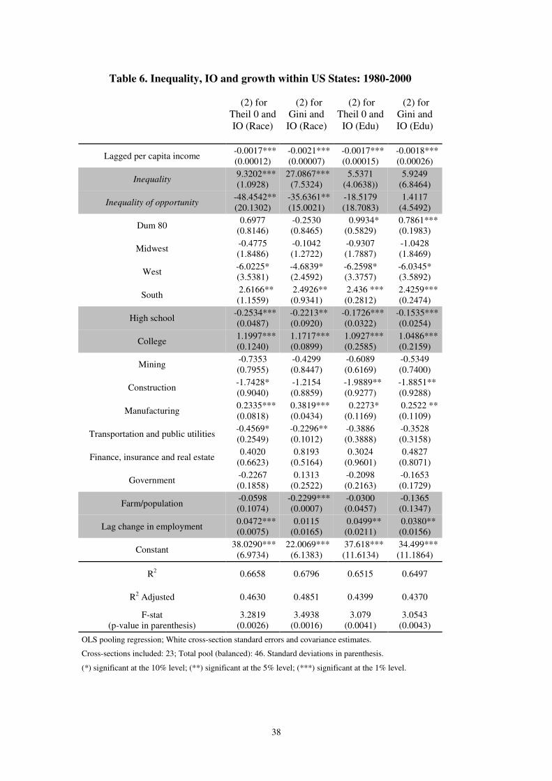
38

Table 6. Inequality, IO and growth within US States: 1980-2000

(2) for

Theil 0 and

IO (Race)

(2) for

Gini and

IO (Race)

(2) for

Theil 0 and

IO (Edu)

(2) for

Gini and

IO (Edu)

Lagged per capita income -0.0017***

(0.00012)

-0.0021***

(0.00007)

-0.0017***

(0.00015)

-0.0018***

(0.00026)

Inequality 9.3202***

(1.0928)

27.0867***

(7.5324)

5.5371

(4.0638))

5.9249

(6.8464)

Inequality of opportunity -48.4542**

(20.1302)

-35.6361**

(15.0021)

-18.5179

(18.7083)

1.4117

(4.5492)

Dum 80 0.6977

(0.8146)

-0.2530

(0.8465)

0.9934*

(0.5829)

0.7861***

(0.1983)

Midwest -0.4775

(1.8486)

-0.1042

(1.2722)

-0.9307

(1.7887)

-1.0428

(1.8469)

West -6.0225*

(3.5381)

-4.6839*

(2.4592)

-6.2598*

(3.3757)

-6.0345*

(3.5892)

South 2.6166**

(1.1559)

2.4926**

(0.9341)

2.436 ***

(0.2812)

2.4259***

(0.2474)

High school -0.2534***

(0.0487)

-0.2213**

(0.0920)

-0.1726***

(0.0322)

-0.1535***

(0.0254)

College 1.1997***

(0.1240)

1.1717***

(0.0899)

1.0927***

(0.2585)

1.0486***

(0.2159)

Mining -0.7353

(0.7955)

-0.4299

(0.8447)

-0.6089

(0.6169)

-0.5349

(0.7400)

Construction -1.7428*

(0.9040)

-1.2154

(0.8859)

-1.9889**

(0.9277)

-1.8851**

(0.9288)

Manufacturing 0.2335***

(0.0818)

0.3819***

(0.0434)

0.2273*

(0.1169)

0.2522 **

(0.1109)

Transportation and public utilities -0.4569*

(0.2549)

-0.2296**

(0.1012)

-0.3886

(0.3888)

-0.3528

(0.3158)

Finance, insurance and real estate 0.4020

(0.6623)

0.8193

(0.5164)

0.3024

(0.9601)

0.4827

(0.8071)

Government -0.2267

(0.1858)

0.1313

(0.2522)

-0.2098

(0.2163)

-0.1653

(0.1729)

Farm/population -0.0598

(0.1074)

-0.2299***

(0.0007)

-0.0300

(0.0457)

-0.1365

(0.1347)

Lag change in employment 0.0472***

(0.0075)

0.0115

(0.0165)

0.0499**

(0.0211)

0.0380**

(0.0156)

Constant 38.0290***

(6.9734)

22.0069***

(6.1383)

37.618***

(11.6134)

34.499***

(11.1864)

R2 0.6658 0.6796 0.6515 0.6497

R2 Adjusted 0.4630 0.4851 0.4399 0.4370

F-stat

(p-value in parenthesis)

3.2819

(0.0026)

3.4938

(0.0016)

3.079

(0.0041)

3.0543

(0.0043)

OLS pooling regression; White cross-section standard errors and covariance estimates.

Cross-sections included: 23; Total pool (balanced): 46. Standard deviations in parenthesis.

(*) significant at the 10% level; (**) significant at the 5% level; (***) significant at the 1% level.

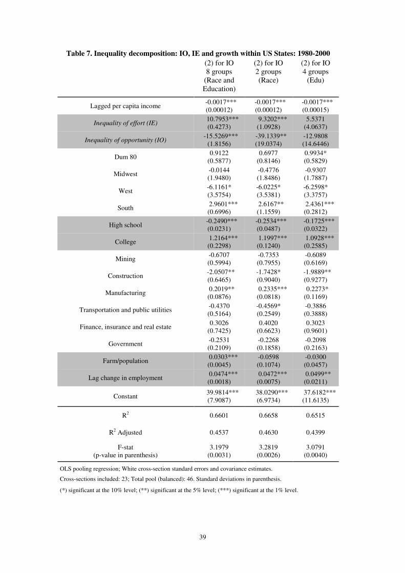
39

Table 7. Inequality decomposition: IO, IE and growth within US States: 1980-2000

(2) for IO

8 groups

(Race and

Education)

(2) for IO

2 groups

(Race)

(2) for IO

4 groups

(Edu)

Lagged per capita income -0.0017***

(0.00012)

-0.0017***

(0.00012)

-0.0017***

(0.00015)

Inequality of effort (IE) 10.7953***

(0.4273)

9.3202***

(1.0928)

5.5371

(4.0637)

Inequality of opportunity (IO) -15.5269***

(1.8156)

-39.1339**

(19.0374)

-12.9808

(14.6446)

Dum 80 0.9122

(0.5877)

0.6977

(0.8146)

0.9934*

(0.5829)

Midwest -0.0144

(1.9480)

-0.4776

(1.8486)

-0.9307

(1.7887)

West -6.1161*

(3.5754)

-6.0225*

(3.5381)

-6.2598*

(3.3757)

South 2.9601***

(0.6996)

2.6167**

(1.1559)

2.4361***

(0.2812)

High school -0.2490***

(0.0231)

-0.2534***

(0.0487)

-0.1725***

(0.0322)

College 1.2164***

(0.2298)

1.1997***

(0.1240)

1.0928***

(0.2585)

Mining -0.6707

(0.5994)

-0.7353

(0.7955)

-0.6089

(0.6169)

Construction -2.0507**

(0.6465)

-1.7428*

(0.9040)

-1.9889**

(0.9277)

Manufacturing 0.2019**

(0.0876)

0.2335***

(0.0818)

0.2273*

(0.1169)

Transportation and public utilities -0.4370

(0.5164)

-0.4569*

(0.2549)

-0.3886

(0.3888)

Finance, insurance and real estate 0.3026

(0.7425)

0.4020

(0.6623)

0.3023

(0.9601)

Government -0.2531

(0.2109)

-0.2268

(0.1858)

-0.2098

(0.2163)

Farm/population 0.0303***

(0.0045)

-0.0598

(0.1074)

-0.0300

(0.0457)

Lag change in employment 0.0474***

(0.0018)

0.0472***

(0.0075)

0.0499**

(0.0211)

Constant 39.9814***

(7.9087)

38.0290***

(6.9734)

37.6182***

(11.6135)

R2 0.6601 0.6658 0.6515

R2 Adjusted 0.4537 0.4630 0.4399

F-stat

(p-value in parenthesis)

3.1979

(0.0031)

3.2819

(0.0026)

3.0791

(0.0040)

OLS pooling regression; White cross-section standard errors and covariance estimates.

Cross-sections included: 23; Total pool (balanced): 46. Standard deviations in parenthesis.

(*) significant at the 10% level; (**) significant at the 5% level; (***) significant at the 1% level.

40

Table 8. The IO and IE components when reducing recursively the number of US States

States IE std p-value IO std p-value

23 All 10.795 0.427 0.000 -15.527 1.816 0.000

22 Arkansas 7.705 1.602 0.000 -15.062 4.814 0.004

21 Tennessee 8.278 1.271 0.000 -13.729 5.760 0.025

20 Kentucky 11.727 5.581 0.047 -11.468 6.527 0.093

19 Iowa 10.591 5.977 0.092 -10.727 4.319 0.022

18 Louisiana 11.831 6.828 0.100 -8.579 4.883 0.096

17 Indiana 24.308 8.808 0.014 -11.051 2.501 0.000

16 Massachusetts 26.465 10.472 0.024 -27.679 16.342 0.112

15 New Jersey 30.515 6.565 0.001 -27.650 14.921 0.089

14 Georgia 46.874 0.7712 0.000 -34.795 7.814 0.001

13 Missouri 60.030 3.195 0.000 -56.266 16.068 0.008

12 Illinois 68.837 4.179 0.000 -154.787 6.209 0.000

11 Florida 70.015 3.933 0.000 -135.742 2.828 0.000

10 Virginia 35.866 4.980 0.019 -89.200 6.042 0.005

41

FIGURES

Figure 1a. Income Inequality in U.S. (1990)

0.00

0.05

0.10

0.15

0.20

0.25

0.30

0.35

0.40

0.45

0.50M

ar

NJe

Ten

Mic

Flo

Tex

USA Lu

i

Ca

l

NC

a

Mis

s

Pe

n

Ge

o

Vir

Oh

i

SCa Ill

Mis

so

Mas Ind

Ke

n

Iow

NY

Ark

Ine

qu

ali

ty

States

Gini

Theil 0

Figure 1b. Inequality of opportunity (8 groups) in U.S. (1990)

0.00

0.05

0.10

0.15

0.20

0.25

0.30

0.35

Ma

r

Ten

Lui

NJe

NC

a

Mic

Vir

SC

a

Mis

s

Ind

Ge

o Ill

Tex

Mis

so Ca

l

US

A

Iow

Ark

Pe

n

Ke

n

Oh

i

Flo

Mas NY

Ine

qu

ali

ty

States

Gini

Theil 0

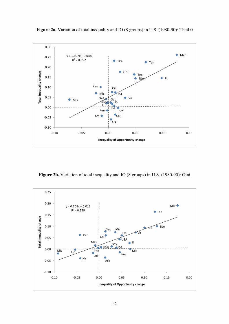
42

Figure 2a. Variation of total inequality and IO (8 groups) in U.S. (1980-90): Theil 0

Ark

Cal

FloGeo

Ill

IndIow

Ken

Lui

Mar

Mas

Mic

Mis

Mio

NJe

NY

NCa

Ohi

Pen

SCa Ten

Tex

Vir

USA

y = 1.407x + 0.048

R² = 0.392

-0.10

-0.05

0.00

0.05

0.10

0.15

0.20

0.25

0.30

-0.10 -0.05 0.00 0.05 0.10 0.15

To

tal

Ine

qu

ali

ty c

ha

ng

e

Inequality of Opportunity change

Figure 2b. Variation of total inequality and IO (8 groups) in U.S. (1980-90): Gini

Ark

Cal

Flo

Geo

Ill

Ind

Iow

Ken

Lui

Mar

Mas

Mic

Mis Mio

NJe

NY

NCa

Ohi

Pen

SCa

Ten

Tex

Vir

USA

y = 0.708x + 0.016

R² = 0.559

-0.10

-0.05

0.00

0.05

0.10

0.15

0.20

0.25

-0.10 -0.05 0.00 0.05 0.10 0.15 0.20

To

tal

Ine

qu

ali

ty c

ha

ng

e

Inequality of Opportunity change