Inequality, Financialisation and Credit Booms: a Model of ...

LUISS Guido CarliSchool of European Political Economy

Working Paper2/2016

Inequality, Financialisationand Credit Booms:

a Model of Two CrisesAlberto Cardaci

Francesco Saraceno

LUISS Guido Carli / School of European Political Economy Working paper n. 2/2016 Publication date: February 2016 Inequality, Financialisation and Credit Booms: a Model of Two Crises

© 2016 Alberto Cardaci, Francesco Saraceno ISBN 978-‐88-‐6856-‐065-‐2

This working paper is distributed for purposes of comment and discussion only. It may not be reproduced without permission of the copyright holder.

LUISS Academy is an imprint of LUISS University Press – Pola s.r.l. a socio unico Viale Pola 12, 00198 Roma Tel. 06 85225485 e-‐mail [email protected] www.luissuniversitypress.it

Editorial Committee: Leonardo Morlino (chair) Paolo Boccardelli Matteo Caroli Giovanni Fiori Daniele Gallo Nicola Lupo Stefano Manzocchi Giuseppe Melis Marcello Messori Gianfranco Pellegrino Giovanni Piccirilli Arlo Poletti Andrea Prencipe Pietro Reichlin

Inequality, Financialisation and Credit Booms:

a Model of Two Crises*

Alberto Cardaci�1 and Francesco Saraceno1,2

1OFCE-SciencesPo, 69 Quai d’Orsay, 75340, Paris, France2LUISS-SEP, Via di Villa Emiliani 14, 00197, Rome, Italy

Abstract

We develop a macroeconomic model with an agent-based household sector and astock-flow consistent structure, in order to analyse the impact of rising income inequal-ity on the likelihood of a debt crisis for different institutional settings. In particular, westudy how economic crises emerge in the presence of different credit conditions and policyreactions to rising income disparities. Our simulations show the relevance of the degreeof financialisation of an economy. In fact, when inequality grows, a Scylla and Charybdiskind of dilemma seems to arise: on the one hand, low credit availability implies a dropin aggregate demand and output; on the other hand, a higher willingness to lend andlower perceptions of system risk result in greater instability and a debt-driven boom andbust cycle. The model allows to replicate the credit-led consumption booms that pavedthe way for both the crisis of 1929 and the recent financial crisis. In addition, our paperyields a new insight on the appropriate policy reaction: tackling inequality by meansof a more progressive tax system compensates for the rise in income disparities therebystabilising the economy. This is a better solution compared to a more proactive fiscalpolicy which, instead, only leads to a larger duration of the boom and bust cycle.

Keywords: Inequality, Household Debt, Credit Markets, Agent-Based Models, Stock-Flow Consistency

JEL Classification: C63, D31, E21, E62, G01

*We are particularly grateful to Tiziana Assenza, Alessandro Caiani, Mauro Napoletano and AlbertoRusso, as well as to the participants at the seminar held in Universita Milano Bicocca, the EEA New Yorkconference, the Bordeaux-Milano Joint Workshop on Agent-Based Models, the 19th FMM Conference inBerlin, the Ancona conference on “Large-scale Crises: 1929 vs 2008”, and the internal seminars at LASER,OFCE and Universite Paris XIII. This paper benefited from funding by the European Community’s SeventhFramework Programme (FP7/2007-2013) under Socio-economic Sciences and Humanities, grant agreementno. 320278 (RASTANEWS).

�Corresponding author, [email protected].

1

©A. Cardaci & F. Saraceno | LUISS School of European Political Economy | Working Paper | 02/2016

1 Introduction: Inequality, Institutions and Financialisation

It is widely established that inequality increased substantially, both in developed and inemerging economies, starting from the late 1970s (Atkinson et al., 2011; IMF, 2007; Mi-lanovic, 2010; OECD, 2008; Piketty and Saez, 2013). In particular, in Europe and in theUnited States those who have lost ground belong to the middle class, while in other areasof the world, such as China, the rise of inequality has hit the very poor. Nonetheless, in allcases the redistribution has benefited mainly the rich and the very rich (the top one percentof the population, see Table 1), giving birth to what Dew-Becker and Gordon (2005) defineas the “Superstar Economy”.

1970 2007 2012

CanadaTop 10% 37.92 40.76 40.12 (2010)Top 5% 24.22 28.46 27.34 (2010)

ChinaTop 10% 17.37 (1986) 27.94 (2003) –Top 5% 9.8 (1986) 17.75 (2003) –

FranceTop 10% 33.14 33.12 32.34Top 5% 21.95 22.33 21.48

GermanyTop 10% 31.8 (1971) 38.57 –Top 5% 22.1 (1971) 27.09 –

ItalyTop 10% 30.5 (1974) 34.12 –Top 5% 19.86 (1974) 23.6 –

JapanTop 10% 31.9 41.03 40.5 (2010)Top 5% 21.13 26.38 25.98 (2010)

SwedenTop 10% 29.36 27.76 27.9Top 5% 18.34 18.06 18.25

UKTop 10% 28.82 42.61 39.13Top 5% 18.65 30.77 27.49

USA Top 10% 31.51 45.67 47.19 (2014)Top 5% 20.39 33.84 34.63 (2014)

Source: The World Wealth and Income Database - WID

http://www.wid.world

Table 1: Top Income Shares for selected countries.

The recent crisis has led to an increasing body of literature, both theoretical and empir-ical, challenging the classical dichotomy between income distribution and economic perfor-mance. In particular, different contributions have identified a link between growing inequalityand the recent financial crisis. In fact, Fitoussi and Saraceno (2010a,b) argue that the rootcauses of the crisis are to be found in the structural weakness of the world economy in 2007.Building on Kaldor’s (1955) framework, Fitoussi and Saraceno notice how the transfer ofresources from lower and the middle people to the wealthiest - i.e. from those who consumealmost all of their income to those who have a high propensity to save - caused a reductionin the average propensity to consume thus increasing the mass of savings. Increased savingsrates have two effects: the accumulation of a large amount of liquidity that fuelled a seriesof speculative bubbles (in the stock and real estate markets); and a chronic deficiency ofaggregate demand. Yet, il line with Fazzari and Cynamon (2013), the authors highlight aparadox, as the generalised increase of inequality does not seem to be correlated to macroe-

2


conomic growth over the decades 1980-2007. For example, in the same years in which incomedisparities widened, the American economy performed reasonably well with sustained con-sumption spending and an average annual growth rate of 3.16% between 1981 and 2007; onthe contrary, other parts of the world, most notably continental Europe, experienced excesssavings and sluggish growth.

The reason why increased inequality led to excess savings in some areas, while resulting inexcesses demand in others, lies in the interaction of the trend in income distribution, commonto all countries, with institutional differences - most notably, the degree of financialisation- and the policy responses that have taken very different forms. As a matter of fact, thedevelopment of financial markets seems to be a key factor that explains such differencesamong countries.

Kumhof et al. (2012) argue that the increase in income inequality in the United Statesand, in general, in more advanced economies, has not been tackled by means of politicalinterventions to support the living standards of those who suffer from stagnating incomes.Rather, policy authorities have temporarily alleviated its consequences “through access tocheap borrowing, in other words through financial liberalization” (Kumhof et al., 2012, p.8). Krueger and Perri (2006) show that the rise in inequality in the United States ledto a change in the development of financial markets, which have allowed households tobetter insure against fluctuations of income. Therefore, in the United States, the reductionin income has been offset by private borrowing, made easier by a less regulated financialsystem, but also by a widespread perception of “end of history” which led to believe thatall constraints to the unlimited growth of some sectors (financial, real estate) had beenpermanently removed. Consequently, aggregate demand remained high, even if it was debt-driven rather than income-driven. Hence, as claimed by Belabed at al. (2013, p. 2), “inadvanced economies with highly developed financial markets, including most notably theUnited States and the United Kingdom, rising inequality has led to a deterioration of nationalsaving-investment balances, as the poor and middle classes borrowed from the rich and fromforeign lenders to finance consumption”. However, growing inequality in other regions ofthe world, such as China, led to a different outcome because “financial markets are lessdeveloped and hence do not allow the lower and middle classes to respond to lower incomes byborrowing” (Belabed et al., 2013, p. 2). The implication is a weaker domestic demand and theemergence of an export-oriented growth model, where richer creditors lend to foreign ratherthan domestic borrowers. Also continental Europe has developed an export-oriented growthmodel, as stricter regulation of financial markets and less accommodating monetary policieshave made borrowing for households and firms more difficult and expensive. PeripheralEurope also experienced a rise in top income shares in the recent decades (Atkinson et al.,2011). However, in contrast with the rest of the continent, these countries recorded growinglevel of household indebtedness as well as current account deficits (Kumhof et al., 2012).

The joint increase of inequality and consumer debt, as well as the resulting financialfragility, are not new in history. Gjerstad and Smith (2014) show that the “Great Recession”of 2008 and the “Great Depression” of 1929 share a similar pattern of real estate appreciation,increasing household debt and booming consumption in the period leading to the financialcrisis, followed by a balance sheet recession in which falling house prices feed back into wealthand consumption contraction. In fact, the initial stage of the crisis in both 1929 and 2008was of strikingly equal intensity (Eichengreen and O’Rourke, 2009): the drop of industrialproduction and of stock market valuations, as well as the shrinking of world trade, weresimilar in size during the first 12-15 months of the crisis. The pattern started to divergeonly when the effects of macroeconomic policies (which were more proactive in the recent

3


crisis) began to materialize. Olney (1999) further stresses that household use of installmentcredit for consumption purposes exploded in the 1920s, in a similar way to the dramaticrise in credit-financed consumption boom prior to the recent Great Recession. The analogyis impressive, as the author points out that outstanding nonmortgage consumer debt morethan doubled in the 1920s, thus making that decade the crucial turning point in the historyof consumer credit. Indeed, “contemporaries noted that in the 1920s it first became commonfor merchants to assume that a customer was buying on credit rather than with cash” (Olney,1999, p. 320-321). After all, in 1930, Persons (1930, p. 94, 96) argued that “the existingdepression was due essentially to the great wave of credit expansion in the past decade”,adding also that “the great field of credit expansion in the last decade lies in the realm ofurban real estate mortgages”. He also highlighted, in line with Olney (1999), the dramaticrise in installment debt used to buy goods such as furniture, clothing and cars.

Fratianni and Giri (2015) further investigate the similarities between the two crises,showing that in both cases monetary authorities’ decisions were the most likely trigger ofthe crisis, as a tightening policy followed a period of monetary expansion. Such point ofview is in line with Rajan (2010), who argued that monetary authorities in the United Statesfostered the speculative boom by implementing an expansionary policy in order to stimulatethe economy, thus facilitating household access to credit markets and sustaining consumptionfor a while, albeit at the price of booming household debt. Rajan emphasises in particularthe role of government failures: “the political response to rising inequality whether carefullyplanned or an unpremeditated reaction to constituent demands was to expand lending tohouseholds, especially low-income ones”, so as to end up with rising household debt. Yet,similar to Fitoussi and Saraceno (2010b), Fratianni and Giri argue that while Rajan may beright in pointing at excessively lax monetary policy as the trigger of the crisis, the role ofthe central bank only led to the amplification of a structural phenomenon, namely wideningincome disparities and increased financial fragility.

The paper is organised as follows: Section 2 introduces our macroeconomic model; Section3 provides an analysis of model results (different institutional scenarios and policy reactions)obtained by means of Monte Carlo repetitions; we also check for the robustness of our resultsthrough sensitivity analysis. Finally, Section 4 concludes drawing hte policy implications ofour investigation.

2 The Model

We build a macroeconomic model with an agent-based household sector. Our goal is toshow how the institutional setting and credit conditions interact with the impact of risinginequality on the performance of the economy and the accumulation of household debt. Wealso investigate whether different policies, which correspond to the choices made by policymakers in the aftermath of the two crises of 1929 and 2008, succeed in stabilising the economy.

Our work follows part of the literature on macro agent-based models. In particular,Cardaci (2014) analyses the consequence of rising inequality in a context of peer effects inconsumption and equity extraction processes. The paper shows that widening income dis-parities result in a debt-financed consumption boom that jeopardises the stability of theeconomic system (a similar result is found in Russo et al., 2015). Our paper represents astep forward. In fact, not only we include an analysis of the impact of inequality for differ-ent degrees of financialisation, but we also assess the effectiveness of different fiscal policyreactions. This is in line with the contribution by Dosi et al. (2013) that focuses on the

4


effect of inequality under different monetary and fiscal policies. They show that more un-equal societies suffer from more severe business cycles oscillations and higher unemploymentrates thus increasing the likelihood of economic crises. Yet, their model only allows for theaccumulation of private debt by firms. On the contrary, we focus on household debt since, aswe showed above, it was a salient feature of the economy before both the 1929 and the 2008crises. On the other hand, this might allow for a generalisation of the policy implications ofour findings.

Our model is also stock-flow consistent (SFC). The SFC approach is commonly used inthe Post-Keynesian literature and dates back to the contributions by Tobin (1969, 1982)and, more recently, Godley and Lavoie (2007). The idea behind this methodology is thattransactions in asset stocks imply the existence of an interlocked system of balance sheets,as Godley and Lavoie (2007) point out. As such, SFC models are built upon an accountingframework whose goal is to coherently integrate all stocks and flows of an economy, so that“every monetary flow, in accordance with the double-entry book keeping logic, is recordedas a payment for one sector and a receipt for another sector, and every financial stock isrecorded as an asset for a sector and a liability for another sector” (Caiani et al., 2014, p.425).

Our model is built upon the “KISS” (Keep It Simple, Stupid!) principle. As such, wedevote our effort to the development of the household sector, while simplifying all the othersas much as possible. Hence, the distinctive features of our economy are as follows:

� There is one representative firm which that produces using labour, and distributes allits earnings.

� In the credit market, a representative bank extends non-collateralised loans to house-holds.

� Households own the firm and the bank. Their desired consumption is based on imitativebehaviour and, more precisely, on the Expenditure Cascades (EC) hypothesis (Franket al., 2014)

� There is a public sector with a government that can issue bonds to finance its deficit(if any), and a central bank.

The model has a sequential structure regarding decisions about flows and actual balance-sheet transactions. The entire sequence of events in each period t can be summarised asfollows:

1. Production. The firm produces homogenous perishable goods using labour as theonly input.

2. Distribution. The firm distributes wages to all households; if the commercial bankhas a positive net worth, its profits are also distributed to households. This process isbased on individual income shares drawn from a Pareto distribution.

3. Bail out. In case of a negative net worth, the commercial bank is bailed out by thecentral bank via a transfer of assets (i.e. reserves).

4. Government revenues and debt. Households pay taxes based on a progressiveand exogenous tax system. Collected taxes add up to the government deposit accountheld by the central bank. The government then pays back its principal and interest onbonds to each household.

5


5. Desired consumption and financial assessment. Households compute their de-sired consumption based on imitative behaviour and assess their own financial position.This latter may be positive, if their internal resources are higher than their desired con-sumption and due debt, or negative, otherwise. Households with a positive financialposition use the exceeding amount of internal resources to demand government bonds,whereas households with a negative financial position ask for a loan.

6. Policy action. Policy institutions their targets: the central bank sets the policyinterest rate while the government sets its desired public expenditure. Both decisionsfollow a counter-cyclical rule based on the value of the “demand gap” in the previousperiod.

7. Bond market. If desired public expenditure exceeds collected taxes and past de-posits, the government needs to borrow from households. Total bond demand simplyequals the sum of individual bond demand by households (see step 5). Note that thebond market may be in disequilibrium since total supply and demand are the result ofindependent decisions.1

8. First pay-back phase (PBP). Households pay back the loan (principal plus inter-est) from the previous period. This does not include borrowers who need to performdebt rollover, as they do not have the internal resources to meet their debt obliga-tions entirely. Hence, they will enter the credit market trying to get a new loan and,afterwards, they will go through a second PBP.

9. Credit market. The bank sets its total available credit supply as a fraction of totalcredit demand and ranks households in ascending order based on their financial sound-ness. Loan applications, computed by households at step 5, are satisfied until thebank exhausts its credit supply. Credit-rationing may occur: more financially fragilehouseholds may not obtain any loan and, as such, they are not be able to finance theirdesired consumption entirely nor to perform debt rollover. Hence, they go bankruptand they are banned from the credit market for an exogenous number of periods.

10. Second pay-back phase. Households who needed debt rollover and successfullyobtained a new loan in the credit market, can now pay back the loan from the previousperiod.

11. Goods market. The government and households buy goods based on their desiredlevel of consumption. If the level of output produced by the firm at step 1 is lower thanoverall desired consumption, rationing takes place. Excess supply, when it appears, isdisposed of at no cost.

12. Macroeconomic closure. Finally, all macroeconomic variables (e.g. GDP, PublicDebt, Private Debt) are updated.

Figure 1 provides a graphical representation of all the transactions taking place in ourartificial economy, based on the sequence reported above. These are represented as flowsfrom a typology of agents to the others. In order to make sure that our model is stock-flowconsistent so that no flow “leaks out” of the system, each agent is provided with a balance

1Note also that we don’t allow for government debt monetisation, so that the amount of deficit is constrainedby savings. This simplifying assumption plays little role, as in the simulations below the supply of governmentbonds is always the short side of the market.

6


sheet that allows us to track and measure the levels of all stock variables at any point intime. Table 2 shows the balance sheets of all the agents in the economy at the end of eachperiod, with the household sector represented in aggregate terms for simplicity.2

Figure 1: Transaction flows in our economy.

Stock-flow consistency implies that any transaction that takes place in the economyis matched by an identical change in the stocks held in the balance sheets of the agentsinvolved. For example, when the firm pays the wage bill, it transfers all of its deposits tothe household sector through the commercial bank. Table 3 provides a numerical example:firm deposits decrease to zero (all revenues are distributed as wages), whereas householddeposits increase accordingly. This transaction is reported also on the liability side of thebalance sheet of the bank. Yet, the net worth of the bank does not change since a transferof deposits does not modify the overall amount of liabilities it holds.3 In general, at theend of each period, agents may have positive or negative individual net worth, depending onthe difference between assets and liabilities. However, stock-flow consistency in our modelimplies that the overall value of the net worth in the economy must always be zero, not only

2Note that central banks do not lend unsecured to commercial banks, as they usually take collateral to protectagainst the possibility of loss due to credit and market risk (Rule, 2015). Yet in our framework, when thecommercial bank is bailed out by the central bank, it receives liquidity (i.e. new assets called reserves)without transferring any assets to the central bank. In other words, our simplifying assumption is that thebailout does not require any collateral or reimbursement and, as such, the central bank does not hold anyasset.

3In principle, such transfer of liabilities takes place among different banks and, as such, it has to be matchedby an equal transfer of reserves on the asset side of their balance sheets. Nonetheless, this change does notoccur in our case because our simplified framework features a single representative bank.

7


Household

Assets Liabilities

Deposits (Dt,H) Loans (Lt,H)Bonds (Bt)

Bank

Assets Liabilities

Loans (Lt,H) Households deposits (Dt,H)Reserves (Rt) Firm deposits (Dt,F )

Firm

Assets Liabilities

Deposits (Dt,F )

Government

Assets Liabilities

Deposits (Dt,G) Bonds (Bt)

Central Bank

Assets Liabilities

Reserves (Rt)Government deposits (Dt,g)

Table 2: Agents’ balance sheets in our economy.

at the end of each period t but also after any transaction.Let us now introduce the rules of behaviour for each category of agent and sector of the

economy.

2.1 Production

The representative firm has a limited role to play in our model: it distributes wages andreacts to disequilibria in the goods market by changing total production. The firm is ownedby the entire population of households, H, who all work for it. As shown in Equations 1 and2, current production (Qt) and prices (Pt) depend on their level in the previous period andon a sensitivity parameter (φQ and φP respectively) multiplied by the demand gap. Thislatter is defined as the previous period difference between aggregate demand and production,divided by production itself, that is gapt−1 = ADt−1−Qt−1

Qt−1. In other words, the demand gap

represents a measure of the real term excess demand or supply in the past.

Qt = Qt−1 (1 + φQ · gapt−1) (1)

Pt = Pt−1 (1 + φP · gapt−1) (2)

At the beginning of each period, the firm distributes its entire revenues, collected at theend of t − 1, to the population in the form of wages. The distribution process is basedon constant individual income shares that are drawn from a Pareto distribution. This is

8


Household

Assets Liabilities

Dt,H = 100 Lt,H = 70Bt = 20

NWt,H = 50

Firm

Assets Liabilities

Dt,F = 80NWt,F = 80

Bank

Assets Liabilities

Lt,H = 70 Dt,H = 100Rt = 110 Dt,F = 80

NWt,B = 0

Household

Assets Liabilities

Dt,H = 180 Lt,H = 70Bt = 20

NWt,H = 130

Firm

Assets Liabilities

Dt,F = 0NWt,F = 0

Bank

Assets Liabilities

Lt,H = 70 Dt,H = 180Rt = 110 Dt,F = 0

NWt,B = 0

Table 3: Numerical example of a wage payment. The firm transfers all of its revenues tothe household sector as wages. This implies a transfer of deposits from the balance sheet ofthe former to that of the latter. This modifies their net worth. Also the bank records thischange on the liability side of its balance sheet, even though its overall net worth remainsthe same.

consistent with empirical evidence suggesting that income is generally distributed accordingto a power-law distribution and, more specifically, to a Pareto, particularly at top of theincome scale (Clementi and Gallegati, 2005; Jones, 2015).

2.2 Expenditure Cascades and Financial Assessment

Individual household income (Equation 3) is defined as the sum of wages (wt,h), profits fromthe bank (πt,h, if any) and the repayment schedule on government bonds from the previousperiod (RSGt−1,h, if any).

yt,h = wt,h + πt,h +RSGt−1,h (3)

After receiving income, households pay taxes based on a progressive tax system, withconstant tax rates set in period 1. Hence, individual disposable income (ydt,h) is given byincome net of the due amount of taxes (Tt,h), as defined in Equation 4.

ydt,h = yt,h − Tt,h (4)

Consumption behaviour in our model is based on peer effects and imitation. This is con-sistent with the empirical literature on behavioural economics, as reported in Cardaci (2014),Fazzari and Cynamon (2013) and Frank et al. (2014). In particular, similar to Cardaci (2014),the formulation of desired consumption in our model follows the Expenditure Cascades (EC)

9


hypothesis introduced by Frank et al. (2014), with a slightly amended formulation (Equation5).

Cdt,h = k · ydt,h + a · Ct−1,j (5)

Therefore, h’s desired consumption is a function of her disposable income (ydt,h) as wellas j’s actual consumption in the previous period, where j is the household who ranks justabove h in the income scale, so that j = h + 1. k is a parameter unrelated to permanentincome level or rank (Frank et al., 2014), while the sensitivity parameter a is such that0 ≤ a ≤ 1: “when a = 1, h fully mimics j’s consumption; whereas when a = 0, h does notconsider j’s consumption” (Cardaci, 2014, p. 8).

As already mentioned, households carry out an assessment of their financial position,by comparing their expected expenditures with their internal resources. That is, if thesum of desired consumption and the repayment schedule on loans from the previous period(RSt−1,h

4) is higher than the sum of their disposable income and past deposits (Dt−1,h),households have a negative financial position and apply for a loan (Ld

t,h) to the bankingsector. That is:

if Cdt,h +RSt−1,h > ydt,h +Dt−1,h

then Ldt,h = Cd

t,h +RSt−1,h − ydt,h −Dt−1,h (6)

On the contrary, households with enough internal resources to finance desired consump-tion and repayment schedule, ask for government bonds (Bd

t,h). Hence:

if Cdt,h +RSt−1,h ≤ ydt,h +Dt−1,h

then Bdt,h = ydt,h +Dt−1,h − Cd

t,h −RSt−1,h (7)

2.3 Bond Market

At the beginning of each period, the government sets its (Gdt ) as a percentage of GDP. As

already pointed out, this decision follows an anti-cyclical rule. In particular, the government

adjusts the initial value of such ratio ( Gd

GDP , computed in period 1) based on its sensitivity(φG) to the demand gap in the previous period.

Gdt

GDPt−1=

Gd

GDP− φG · gapt−1 (8)

Afterwards, the government carries out its own financial assessment by computing thedifference between its expected expenditure (the sum of desired public expenditure and therepayment schedule on public bonds issued in the previous period, RSGt−1) and its availableinternal resources (the sum of past deposits, Dt−1,g, and the amount of taxes collected, Tt).If this is negative, the government has enough resources to finance the expected expenditure.On the contrary, if the difference is positive, the government has to finance its expenditureby issuing new public bonds. The overall supply of bonds is defined in Equation 9.

4The repayment schedule on loans is defined in section 2.4.

10


BSt = Gdt +RSGt −Dt,g (9)

Note that government deposits at time t are defined as the sum between past deposits andtax revenues, so that Dt,g = Dt−1,g+Tt. We assume that bonds are one period debt contractsbetween households and the government. Hence, in the following period, the government willpay back RSGt−1, which includes both principal and interests. We also make the assumptionthat the interest rate on bonds is equal to the policy rate set by the central bank (see Section2.4).

It is wort noting that there is no mechanism that guarantees that the bond market isin equilibrium. In other words, as the formulation of bond demand and supply are basedon independent decisions by households and the government, rationing may take place inthe bond market. Indeed, if total bond supply is higher than demand, all households askingfor bonds get the desired amount. Still, in the opposite case, all applicants are rationedso that the amount each h gets is equal to Bd

t,hBStBDt

, where BDt is total bond demand (i.e.

BDt =∑

hBdt,h).

2.4 Pay Back Phase and Credit Market

As pointed out in Section 2.2, only households with a negative financial position enter thecredit market. Note, however, that we distinguish two types of borrowers: consumptionborrowers (CB) and borrowers in financial distress (FDB). CB are all households whose ownresources are enough to pay back their repayment schedule on the loan from the previousperiod5. Hence, they enter the market in order to get a loan to finance their desired con-sumption only. On the contrary, FDB ask for a new loan not only to finance consumptionbut also to perform debt rollover. In other words, FDB use the new loan to pay back theprevious one.

The commercial bank sets a maximum allowable credit supply as a fraction of total creditdemand (Equation 10).

LSt = vt∑h

Ldt,h (10)

Note that vt ∈ [vmin, vmax]. That is, the commercial bank endogenously changes the valueof vt within two boundaries (vmin and vmax) that are exogenously set in the initialisationphase of the model (Conditions 11 and 12). In particular, vt evolves as a function of systemic

risk which is proxied by the household debt-to-GDP ratio in the previous period, debtt−1

GDPt−1.

In fact, we introduce an exogenous parameter (threshold) that represents the sensitivitythreshold to the level of the household debt-to-GDP ratio, so that if the ratio is higher(lower) than the threshold, the bank decreases (increases) vt.

if debtt−1

GDPt−1> threshold then vt = vt−1 − φv(vmin − vt−1) (11)

if debtt−1

GDPt−1< threshold then vt = vt−1 + φv(vmax − vt−1) (12)

The sensitivity threshold, as well as the two boundaries for vt, represent our key pa-rameters in the simulation phase of the model as they act on the willingness to lend of the

5CB also includes households with zero repayment schedule, that is, those who did not take any loan in t− 1.

11


commercial bank and on its reaction to systemic risk. Hence, a more financialised economyis one in which both threshold and vmax are set to high values.

The commercial bank ranks households in ascending order based on a measure of theirfinancial soundness - namely the total debt service ratio (TDS)6 - and supplies credit bymatching each individual demand until LSt = 0. As a consequence, if vt < 1, less financiallysound applicants (namely, households with a higher TDS) will be rationed on the creditmarket thus getting no loans at all. Borrowers who are credit-rationed cannot pay back theirprevious loan and, in some cases, finance their desired consumption entirely. Therefore, theywill go bankrupt and as such they are not allowed to apply for another loan for a limitedperiod of time.

Similar to bonds, we assume each loan is a one-period debt contract corresponding to arepayment schedule defined as RSt,h = Lt,h(1+rLt,h), to be paid back entirely in the followingperiod. Similar to Russo et al. (2015) and Cardaci (2014), the interest rate on loans is madeup of three components, as described by Equation 13.

rLt,h = rt + rt + rt,h (13)

rt is a system-specific component that reflects the sensitivity of the bank to the householddebt-to-GDP ratio of the economy, so that rt = ρ debtt−1

GDPt−1, while rt,h is a household-specific

component equal to µTDSt,h, where µ is the bank sensitivity to household total debt serviceratio. Finally, rt is the policy rate set by the central bank at the beginning of each period(Equation 14). Similar to desired public expenditure, the central bank reacts to changes inthe demand gap.7

rt = rt−1 + φCB · gapt−1 (14)

Once transactions in the credit market are over, a new PBP begins: all FDB who suc-cessfully got a loan now pay back their due debt RSt−1,h.

2.5 Goods Market

Both the government and households interact with the firm in order to buy goods. Notethat each agent on the demand side may have an actual capacity of spending that differsfrom the desired one. As a matter of fact, even though the government is willing to spendan amount equal to Gd

t , it is possible that its liquidity does not allow to do so and its actualspending capacity is constrained by its current deposits (Dt,g), which include collected taxes,issued bonds and past deposits. Hence actual maximum government expenditure is definedas min(Gd

t , Dt,g). Similarly, some households might not be able to finance their desiredconsumption entirely due to credit rationing, as already pointed out. As a consequence,actual maximum expenditure for each household is equal to min(Cd

t,h, Dt,h).Before transactions take place, the firm compares aggregate demand in real terms (Equa-

tion 15) with the amount of quantities produced.

ADt =min(Gd

t , Dt,g) +∑

hmin(Cdt,h, Dt,h)

Pt(15)

6Following Cardaci (2014), TDS is defined as the ratio between household repayment schedule and disposableincome.

7As quantities and prices move in the same direction, the central bank is implicitly targeting inflation as well.

12


If the former is lower than the latter, each buyer will obtain the demanded amount ofgoods, while the firm will get rid of excess supply at no cost. In the opposite case, instead,all buyers in the goods market will be rationed. If such a circumstance occurs, the firmcomputes a “rationing ratio” equal to Qt

ADt. This applies equally to the government as well

as each household, so that all buyers are rationed in the same way and actual householdconsumption and government spending are defined as Ct,h = min(Cd

t,h, Dt,h) Qt

ADtand Gt =

min(Gdt , Dt,g) Qt

ADt.

3 Model Results

Model results are obtained by means of computer simulations. We start by replicating thefollowing three scenarios:

� a baseline (BS) scenario with income shares that are fixed at the beginning of the firstperiod and remain constant over time;

� a rising-inequality (RS) scenario in which we change the value of individual incomeshares over time to simulate increasing income disparities;

� finally, a credit-inequality (CS) scenario in which the maximum propensity to lend ofthe bank rises along with the same rise of inequality simulated in RS.

We also run some additional experiments to assess different model dynamics when finan-cial conditions, as well as policy implementations, change.

For each scenario we perform 20 Monte Carlo (MC) repetitions selecting a differentrandom seed at each run, similar to Delli Gatti et al. (2011) and Russo et al. (2015). Thechoice of our parameter vector, shown in Table 4, is based on the need to rule out explosivedynamics and unrealistic patterns, so that “no attempt has been made at this stage tocalibrate the model for instance, by means of genetic algorithms in order to force the outputof simulation to replicate some pre-selected empirical regularities” (Delli Gatti et al., 2011,p. 61). Moreover, we perform both univariate and multivariate sensitivity analysis in orderto test the robustness of model results to changes in parameter values.

3.1 Monte Carlo Analysis of the Three Scenarios

For each scenario, we compute the cross-simulation mean of the key variables. For example,we calculate GDP at each time t as the average of GDP across the 20 MC ripetitions foreach of the three scenarios. Moreover, we drop the first 200 periods in order to get rid oftransients, that is the stabilisation phase of the model. Graphs only show the last 800 periodsfor this reason. Furthermore, following Cardaci (2014), all data generated by our model arerepresented as simple moving averages in order to smooth out the cyclical fluctuations of thetime series.

BS is based on the calibration shown in Table 4, while in the other two scenarios weimplement the following shocks:

� RS: the income share of the top 10% increases gradually (from period 401 to period600) from 22% to 37%.

� CS: we perform the same inequality shock as in RS, together with a sudden rise invmax which increases from 0.4 to 0.8 in period 401.

13


Parameter Value

T Number of periods 1000H Number of households 200k Propensity to consume for h = 1 : H − 1 0.8kH Propensity to consume for h = H 0.6a Sensitivity parameter to j’s past consumption 0.6

vmax Maximum propensity to lend 0.4vmin Minimum propensity to lend 0.1ρ Bank sensitivity to debt/gdp ratio 0.005µ Bank sensitivity to TDS 0.005φQ Output sensitivity to output gap 0.01φP Price sensitivity to output gap 0.01φG Government sensitivity to output gap 0.05φCB Central bank sensitivity to output gap 0.05φv Speed of adjustment for credit supply 0.05

freeze Number of “freezing” periods for bankrupt borrowers 5threshold Bank threshold for debt-to-GDP ratio 0.5

Table 4: Model calibration

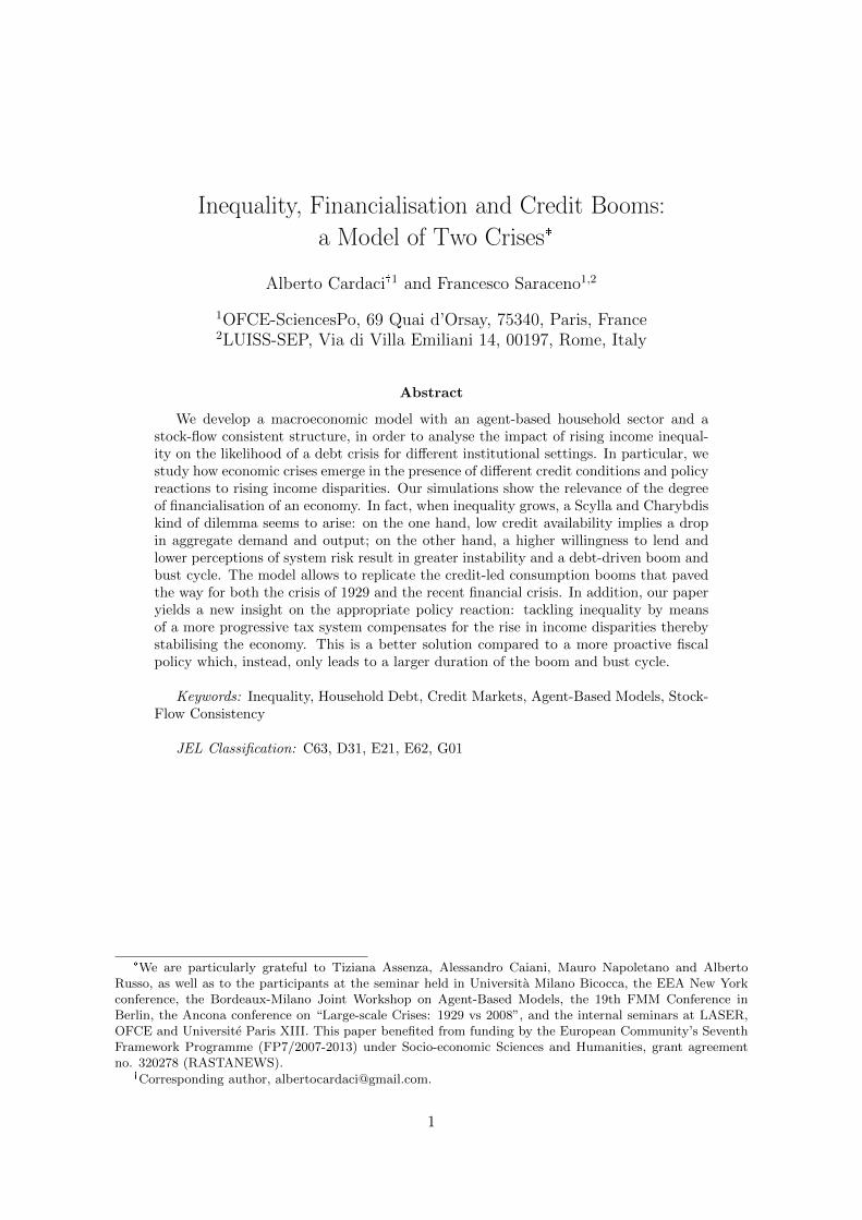
All the key time series obtained by means of MC repetitions show smooth and minoroscillations along a stationary trend in the baseline scenario (as confirmed by Table 5, whichreports also the average growth rates of GDP in all the 20 MC simulations for the baselinescenario). In particular, the model seems to stabilise along a quasi-steady state. As shownin Figure 2, GDP in BS is rather flat over time.

Let us provide a narrative for the other two scenarios.

� RS. Figure 2 shows quite distinctly that a rise in income disparities results in fallingGDP. As a matter of fact, when income moves from the bottom to the top of thedistribution, overall desired consumption rises for a very small number of periods dueto stronger expenditure cascades. However, financial parameters (vmax, thresholdand φv) in RS do not change compared to their baseline values and the economyremains poorly financialised as it is in BS. As a consequence, households do not findenough credit supply to finance their increased desired expenditure and demand forloans. Indeed, in the baseline the household debt-to-GDP ratio is well below the banksensitivity threshold and, consequently, vt rises endogenously up to vt = vmax, ∀t. Thatis, in BS the banking system endogenously increases its willingness to lend up to itsmaximum value as it detects low systemic risk. Yet, as vmax is calibrated at a lowvalue in BS and RS (see Table 4), the result of increasing inequality in our economywith a low degree of financialisation and credit availability is a recession with fallingdebt and desired consumption.

� CS. Similar to RS, as soon as income inequality starts to increase, household desiredconsumption grows because of stronger imitation effects. However, the degree of finan-cialisation is different in CS, as the commercial bank has a higher maximum willingnessto supply credit. That is, a greater value of vmax allows vt to rise endogenously so thata broader number of borrowers actually finds the necessary external resources to fi-nance their desired spending. In fact, even if income disparities become wider, GDP

14


SimulationAverage growth

rate (%)Mean Variance

StandardDeviation

1 1.51 15443.80 2848.26 53.372 1.31 15685.65 8572.67 92.593 1.11 15382.01 3138.18 56.024 0.17 15636.93 4992.87 70.665 0.61 15593.71 3554.80 59.626 1.47 15639.42 8035.21 89.637 1.03 15416.06 5673.53 75.328 0.89 15428.54 3084.45 55.549 0.97 15415.67 2321.31 48.1810 1.09 15518.28 5624.1 74.9911 1.07 15606.42 4321.62 65.7412 0.3 15200.34 2895.02 53.813 0.76 15752.72 3546.91 59.5514 1.39 15536.94 5783.84 76.0515 0.19 15516.43 2847.19 53.3616 0.35 15491.02 4382.62 66.217 1.1 15574.72 9465.53 97.2918 0.72 15592.42 3043.92 55.1719 1.16 15484.07 2836.83 53.3620 0.36 15471.21 2838.9 53.28

Table 5: Key statistics for BS-GDP in the 20 MC simulations.

rises in CS as a result of debt-financed consumption. Also note that the default rate ofborrowers actually goes down. This is not surprising: higher credit availability resultsin a greater number of households who successfully perform debt-rollover and as suchmore borrowers are actually able to pay back their older loans. Nonetheless, this alsoimplies that household debt grows faster than GDP: the debt-to-GDP ratio increasesas well, going beyond the threshold level set by the commercial bank. This is theturning point: the bank starts decreasing its willingness to lend and, as a consequencethe portion of overall credit demand that is actually matched by credit supply dropsthus triggering the recession. Two aspects are worth stressing: (1) the fall in GDPis slower than that of desired consumption and (2) credit demand and supply remainsubstantially higher compared to their baseline level, even though they both experi-ence much wider oscillations along a roughly decreasing trend. The first point canbe explained by the impact of public spending which decreases but at a fairly slowerrate than private spending. The second point, instead is explained by looking at thenumber of households who need debt rollover, which remains stable at around 60%after the peak of GDP and debt. This entails a change in the nature of credit: thehigher demand for credit after the recession comes from FDB and it is, as such, fordebt rollover purposes rather than for consumption financing.

3.2 Financialisation and Institutional Setting

The results of our three main scenarios suggest that where credit constraints are relaxed,higher loan demand can be matched by a wider availability of credit thereby resulting in

15


Figure 2: GDP (top left), aggregate desired consumption (top right), household debt (bottomleft) and household debt-to-GDP (bottom right) in BS (blue), RS (red), CS (yellow).

higher household debt that sustains aggregate demand at the price of greater instability;whereas, if access to credit is harder and its availability is subject to tighter regulation,widening income disparities are not compensated by increased borrowing and, as such, theeconomy performs badly.

We now want to provide a deeper analysis of the impact of growing inequality on theperformance of the economy under different degrees of financialisation. To do so, we run twomore sets of simulations by randomly drawing 20 different values for vmax and threshold.For each of these values, we also perform 20 MC repetitions, each with a different randomseed (for a total of 400 simulations).

In the first case we reproduce a multitude of scenarios where the bank has a differentmaximum willingness to lend, while in the second case we test how greater credit availabilityinteracts with different sensitivities to the household debt-to-GDP ratio by the bank.

Let us start from changes in vmax. When inequality rises, we increase the maximumwillingness to lend of the bank without changing the value of threshold or any other pa-rameter in the model. Figure 3 reports our key results for selected values of vmax. Thegraphs show that a higher value of vmax corresponds to a greater boom and bust cycle, asexpected. That is, a stronger degree of financialisation allows for more debt-financed desiredconsumption by households, while a lower amount of credit availability forces the economyinto the recession since the downward pressure on the aggregate demand is not compensatedby higher household debt.

16


Figure 3: GDP (left) and aggregate desired consumption (right) for vmax equal to 0.5724(purple), 0.5846 (green), 0.6023 (light blue), 0.6894 (dark red), compared to baseline (blue),RS (red) and CS (yellow).

Figure 4: GDP (left) and aggregate desired consumption (right) for threshold equal to 0.1048(green), 0.2041 (purple), 0.2533 (light blue), 0.3705 (dark red) compared to baseline (blue),RS (red) and CS (yellow).

Next we investigate the case of a different threshold in CS. That is, when inequalityincreases, the bank is willing to supply more credit, since vmax jumps from 0.4 to 0.8 inCS, but it also has different sensitivities to the household debt-to-GDP ratio (starting fromperiod 1 and letting the other parameters unchanged). Our results for selected values ofthrehsold are shown in Figure 4. Clearly, threshold is a key parameter in determiningmodel dynamics. As a matter of fact, lower values of threshold imply a worse performanceof the economy, regardless of the increased willingness to lend of the bank. In particularwhen threshold is less or equal to 0.1, the economy in CS performs even worse than in theRS scenario where threshold = 0.5 and vmax = 0.4. In general, our findings seem to bringabout further evidence that the degree of financialisation matters, even when we look atanother dimension, namely the sensitivity of the commercial bank to systemic risk.

17


Figure 5: GDP (top left) and aggregate desired consumption (top right) for different levels ofprogressive tax system (purple, green and light blue) compared to baseline (blue), RS (red)and CS (yellow).

3.3 Policy Responses

We now move on to the analysis of different policy interventions. In particular, we compare a“Keynesian” type of policy - consisting in a bolder reaction of desired government expenditureto the demand gap8 - with an increase in “progressivity” of the tax system that tacklesinequality by redistributing income from the top to the bottom of the population. Ourresults suggest that the second type of policy has a clearer and stronger effect on the overalleconomy with respect to an intervention of the first type.

Simulations are carried out following the same procedure introduced above: we randomlydraw 20 different values for φG and for each of them we also perform 20 MC repetitions ineach of the three scenarios (hence, we perform 1200 computer simulations in total). We findthat, a greater value of φG does not avoid the recession that results from rising inequalityin the RS scenario. Moreover, in the CS scenario, that is when inequality rises togetherwith the maximum willingness to lend of the banking system, the impact of the Keynesianpolicy reaction is non tangible. That is, the time series for the key variables do not showany significant difference (in terms of magnitude, duration and volatility of the boom andbust cycle) compared to the standard time series obtained in the CS scenario with φG equalto its baseline value.

What happens if, instead, the government reacts to rising inequality by changing thetax rates such that it redistributes income from households at the top of the distribution tothose at the bottom? In this case, the impact on the economy is strong and positive. Notethat we analyse the fiscal reform in RS so that all model parameters, including the financialones, do not change.

Selected simulations are reported in Figure 5. They all show that more progressivesystems manage to counterbalance the (exogenous) change in the Pareto distribution thatalters the original distribution of income. Regardless of the degree of progressivity, theeconomy has a higher and more stable GDP compared to the baseline, as well as a similar levelof household debt. This latter is also much lower than in CS. In any case, a more progressivetax system results in a dramatic boom in GDP followed by a prolonged period of stability.

8Notice that in our model “Keynesian” does not indicate a large government, but rather a proactive one. Ourinterpretation is consistent with the first part of the General Theory.

18


This is not surprising: by counterbalancing the rising trend in inequality, the governmentprovides poorer households with the necessary internal resources to finance their desiredconsumption. As a consequence, the household sector relies much less on debt accumulationso that both household debt and household debt-to-GDP stabilise around the baseline levelafter a certain number of periods.

As far as our result seem to push in favour of a structural reform with a more progressivetax system, for the sake of completeness it is worth pointing out that we do not take intoaccount any consideration regarding the distortionary effect that greater progressivity mayhave on other aspects of the economy, such as the functioning of labour markets or firmprofits and investment decisions. The interpretation of our results should therefore be lim-ited to considering that an increase in progressiveness is more efficient than macroeconomicpolicies in tackling the expenditure cascades that follow an rise in inequality. Any furtherinterpretation would be unwarranted given the simplified structure of our model.

3.4 Consumption and Income Inequality

One of the major advantages of agent-based models is that they allow to track and analysethe distribution of key economic variables among the population of the artificial economy. Inparticular, we are interested in assessing how consumption and income inequality change inthe three basic scenarios introduced above. Notice that even though wages and bank profitsare distributed based on exogenous Pareto shares, interests on government bonds are basedon the stock of bonds held by each household. As such, they might allow income distributionto change endogenously.

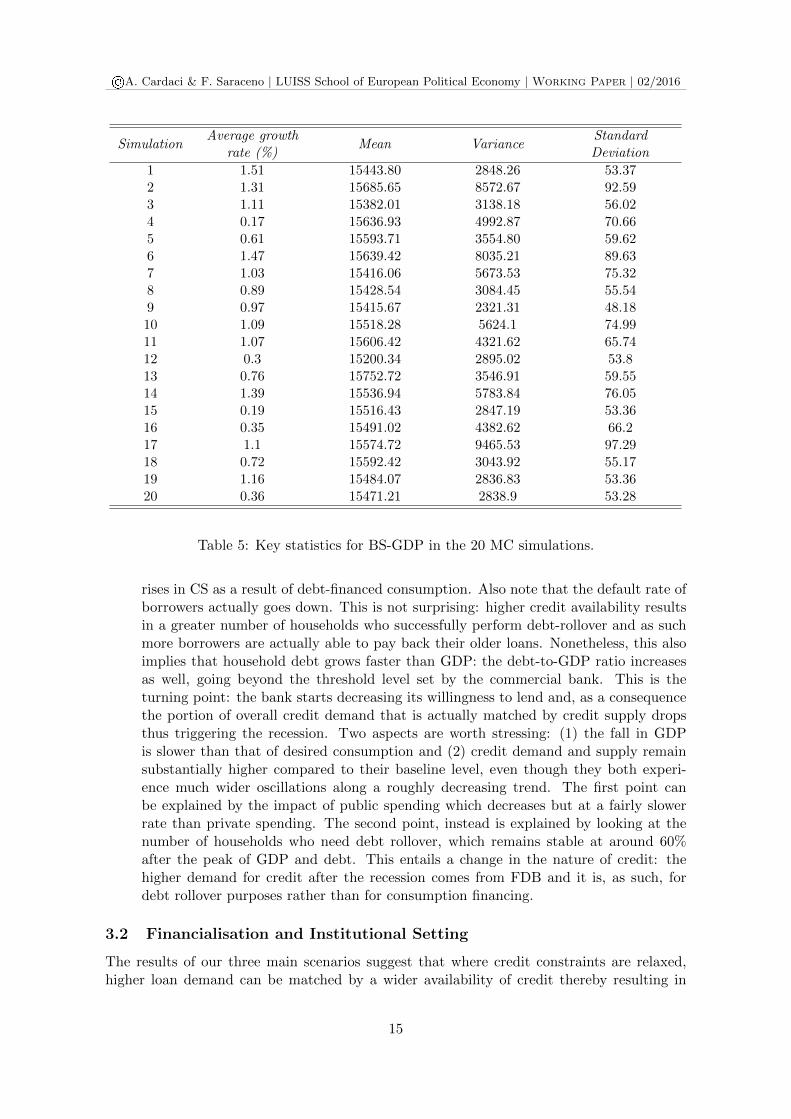
In order to measure consumption (income) inequality we compute the ratio betweenactual consumption (disposable income) at the richest 20% and at the poorest 20% of thepopulation. Figure 6 plots the time series of such ratios in BS, RS and CS.

In the BS scenario, the distribution of both consumption and income remains fairly con-stant. Following the inequality shock in both RS and CS, the two measures of distributionrise, thus indicating a stronger concentration of income and consumption at the top. Yet,income inequality is lower in CS compared to RS. This is explained by looking at the timeseries of household consumption for the same percentiles. These are reported in Figure 7,which shows that households at the top increase their consumption in CS, thereby accumu-lating lower savings and, consequently, government bonds. As such, interest income increasesless than in the RS scenario thus contributing to a lower increase of income inequality inCS compared to RS. As expected, also consumption inequality is lower in CS with respectto RS. This is explained by the greater availability of credit to poorer households in theexpansionary phase of the economy.

In general, one can observe that consumption inequality tracks income inequality in allscenarios, a behaviour that is confirmed by recent empirical analysis (Aguiar and Bils, 2011).

3.5 Sensitivity Analysis

In order to check whether our model results are biased by the specific combination of param-eter values, we perform both univariate and multivariate sensitivity analysis. This allows usto test the robustness of the model following changes in the parameter vector.

Univariate analysis consists in assessing variations in model outcome while performingchanges in one parameter at a time, leaving all the others constant. As Delli Gatti et al.(2011, p. 77) point out, “the model is then believed to be good if the output values of interestdo not vary significantly despite significant changes in the input values”. Hence, we select

19


Figure 6: Consumption (top) and income (bottom) inequality in BS (blue), RS (red) andCS (yellow).

12 parameters of our model and we randomly draw 20 values within a reasonable min-maxinterval for each individual parameter at a time, leaving all the other ones unchanged. Then,for each of the 20 values, we perform 20 MC repetitions, each with a different random seed,in the 3 scenarios (BS, RS and CS). Therefore, the univariate analysis of a single parameterimplies 1200 simulations. Since we explore 12 parameters, we run 14400 simulations in total.

As a general comment, we highlight that for most variables the resulting variations inoutput are smaller than the variations in the parameters. This indicates that results areindeed quite robust with respect to univariate changes in model parameters. Table 6 reportsthe variation for each parameter between its minimum and maximum value in the sensitivityanalysis and the corresponding cross-series variation in GDP at time 500 for BS and attime 1000 for RS and CS9. With the only exception of a and k, output variations in thebaseline scenario are consistently small for a very wide range of values for each individualparameter. Notice that variations in two parameters, namely vmax and φv, do not determineany change in output in BS. Univariate analysis also shows that individual changes in a widerange of model parameters have no significant effect on the dynamics of the model in theRS scenario either, even though freeze has a slightly more relevant role than in BS. Finally,as expected, all parameters have a more distinctive impact on model dynamics in CS: our

9For the sake of simplicity, we report values for GDP only since our results show that variations in the otherkey time series are in line with those for GDP.

20


Figure 7: Household consumption for the poorest 20% (top) and richest 20% (bottom), inBS (blue), RS (red) and CS (yellow).

analysis confirms the primary role of the consumption parameters, a and k, as well as of thefinancial parameters related to the behaviour of the banking system, namely threshold andvmax, followed by φv and freeze.

The univariate analysis for the CS scenario shows that values of a between 0.4 and0.6 result in shorter booms and longer busts, whereas a > 0.6 implies a wider durationof the expanding phase of the economy. In addition, values of k lower than 0.5 seem tocounterbalance the impact of a higher willingness to lend, as the CS scenario collapses tothe RS in this case. a and k are not the only relevant parameters in CS. As a matter offact, our results suggest that φQ, φP , φv, threshold and freeze have an impact on modeldynamics in this scenario as well. In particular, higher values of φQ and φP imply greaterbooms and faster recessions. Higher values of φv and freeze result in faster and strongerbooms and longer busts over time, whereas the higher threshold, the greater and longer theboom before the bust.

As a further robustness check, we also compute the percentage of successful simulationsfor each of the parameters tested in the univariate analysis. We do so by calculating themean and the variance of selected key variables (i.e. GDP, desired consumption, householddebt, credit demand and household default rate) along the entire time span in each of thethree scenarios. Then we compare these values, obtained under the different calibrationsused in the sensitivity analysis, with the same values obtained with the standard calibrationreported in Table 4.

For example, based on the standard calibration, both the mean and the variance ofGDP are lower in RS and higher in CS, compared to the baseline values. Hence, we checkwhether GDP has the same qualitative behaviour in terms of mean and variance in any

21


ParameterVariation in

parameter (%)

Variation inGDP-BS at t 500

(%)

Variation inGDP-RS at t

1000 (%)

Variation inGDP-CS at t

1000 (%)

k 65.1 12.68 25.60 102.18a 302.64 28.4 60.37 231.22

vmax 103.56 0 0 53.69ρ 355.25 1.3 2.15 14.38µ 2505.26 0.39 1.59 19.39φQ 1369.17 0.98 3.47 22.05φP 1817.82 1.73 3.69 14.36φG 274.37 2.38 1.59 9.71φCB 288.55 1.22 1.39 14.08φv 747.62 0 0 34.72

freeze 350 3.42 10.02 30.9threshold 660.69 0.45 0.54 59. 44

Table 6: Min-max variations in parameter values for univariate sensitivity analysis, togetherwith corresponding cross-series variation in GDP at time 500 in BS and at time 1000 in RSand CS.

other univariate simulation. For instance, we find that, ceteris paribus, any of the randomlyselected values of ρ implies that both the mean and variance of GDP are lower in RS andhigher in CS. Hence, we claim that 100% of the univariate simulations for ρ are successful.

We repeat this experiment for all the parameters tested in the univariate analysis (Table7) and we find that, on average, 98.96% of univariate simulations are successful, based onthe criteria mentioned above. This is further evidence that the model is fairly robust tounivariate changes in model parameters.

ParameterSuccessful

simulations (%)Parameter

Successfulsimulations (%)

k 97.91 φG 100a 98.75 φCB 100

vmax 100 φv 100ρ 100 vmax 94.63µ 100 threshold 96.3φQ 100 freeze 100φP 100

Average 98.96

Table 7: Percentage of successful simulations in the univariate sensitivity analysis.

Multivariate analysis tests changes in model results with different calibrations of modelparameters. In this case, we build 20 parameter vectors for our model parameters. Eachvalue in the vector is randomly draw within a reasonable interval. Then, for each of the20 vectors, we perform 20 MC repetitions, each with a different random seed, in the threescenarios. Hence, in the multivariate sensitivity analysis, we run 1200 simulations in total.

The multivariate analysis shows that the behaviour of the model is robust to parameter

22


Figure 8: GDP in the multivariate sensitivity analysis.

changes. Figure 8, which shows GDP for each of the parameter vectors, proves that almostany combination of parameters leads to the same dynamics from a purely qualitative point ofview. The only exception to this is represented by the highest blue line in the graph (Figure8): in CS, for this specific combination of parameters, GDP booms in the expansion phaseof the economy while falling at a dramatically slow pace during the recession. By lookingat the calibration for this particular case, one may have an intuition about such dynamics:this scenario features a value of a and k close to 1, a very low value of freeze (equal to2), as well as a higher threshold (around 0.6) and a much greater value for vmax (around0.8). We believe that the explanation for the entity of the boom, as well as its sensationallyslow negative growth in the recession, is to be found precisely in the extremely large valuesof a, k and vmax that allow the model to follow the same dynamics as in the standard CSwith more pronounced values. In other words, GDP booms as a consequence of strongerexpenditure cascades and greater availability of credit. However, after peaking, the economyenters a recession and GDP starts to fall. Its remarkably small negative growth rate mightbe the consequence of very low value of freeze as it implies easier access to credit marketsfor both consumption and debt-rollover purposes. In other words, even though the banklowers its endogenous willingness to lend, households who go bankrupt can still access thecredit market after a very few periods and, as such, debt-financed consumption keeps goingon during the recession (even though at a lower speed compared to the boom).

With the exception of the above mentioned case, we can generally conclude that resultsfrom our simulations are in line with those for the univariate case. That is, our multivariatesensitivity analysis confirms the primary role of just a few model parameters, namely aand k in determining model dynamics in BS and RS. It also highlights the importance ofvmax and threshold in the CS case, thus proving the importance of reproducing alternativefinancial and policy scenarios by changing the values of such parameters. In addition, wecompute the percentage of successful simulations also in the multivariate case. Based on the

23


same criteria described for the univariate analysis, our test identifies 86.25% of successfulsimulations in the multivariate case, thus leading us to conclude that the model is robustalso to multivariate changes in model parameters.

4 Conclusion

Through an agent-based macroeconomic model with a stock-flow consistent structure, weshowed how different institutional settings and levels of financialisation affect the dynamicsof an economy hit by an increase of inequality. In fact, when income disparities becomewider, a dilemma arises. That is, when the degree of financialisation is poor and financialinstitutions are less willing to lend, increasing inequality implies a drop in aggregate demandand output. On the contrary, when credit constraints are relaxed and the financial sectoris prone to lend, our results spotlight a short term positive effect on growth at the price ofgreater financial instability, in line with Kumhof et al. (2012) and Russo et al. (2015). Hence,the model allows to replicate the credit-led consumption boom that paved the way for therecent financial crisis as well as that of 1929.

In addition, our paper yields a new insight on the comparison between the Great De-pression of the 1930s and the recent crisis. Indeed, there is little doubt that the lessonslearned from the policy mistakes of the Great Recession allowed, at least in some countries,to counterbalance the recent bust with effective monetary and fiscal policies (where coun-tercyclical policies were not massively used, as for example in Europe, the crisis was longerand deeper). Nevertheless, our paper shows that another lesson should be learned: withoutstructural policies aimed at restoring more equal societies, the fragility of the economy willpersist beyond the current crisis. The return to more equal societies that followed the greatrecession played a major role in the sustained growth of the post-WWII period (Piketty,2013). Our results suggest that the substitution of structural policies aimed at rebalancingincome distribution with proactive fiscal (and monetary) policies is bound to fail at stabil-ising the economy beyond the short term. There is no way around a serious reconsiderationof the mechanisms for distributing wealth and income. Therefore, in order to avoid beingcaught between the Scyilla of stagnant growth and the Charybdis of instability, it seemsnecessary to act on the structure of the economy and on the problem of inequality at itsroots.

References

Aguiar, M. A. and Bils, M. (2011). Has consumption inequality mirrored income inequality?Working Paper 16807, National Bureau of Economic Research.

Atkinson, A. B., Piketty, T., and Saez, E. (2011). Top incomes in the long run of history.Journal of Economic Literature, 49(1):3–71.

Belabed, C., Theobald, T., and Van Treeck, T. (2013). Income distribution and currentaccount imbalances. IMK Working Paper, (126).

Caiani, A., Godin, A., and Lucarelli, S. (2014). Innovation and finance: a stock flowconsistent analysis of great surges of development. Journal of Evolutionary Economics,24(2):421–448.

24


Cardaci, A. (2014). Inequality, household debt and financial instability: an agent-basedperspective. Working paper.

Clementi, F. and Gallegati, M. (2005). Pareto’s law of income distribution: Evidence forgermany, the united kingdom, and the united states. In Chatterjee, A., Sudhakar, Y., andChakrabarti, B. K., editors, Econophysics of Wealth Distributions. Springer Milan.

Delli Gatti, D., Desiderio, S., Gaffeo, E., Cirillo, P., and Gallegati, M. (2011). Macroeco-nomics from the Bottom-Up. Milano, IT: Springer.

Dew-Becker, I. and Gordon, R. J. (2005). Where did the productivity growth go? inflationdynamics and the distribution of income. Brookings Papers on Economic Activity.

Dosi, G., Fagiolo, G., Napoletano, M., and Roventini, A. (2013). Income distribution, creditand fiscal policies in an agent-based keynesian model. Journal of Economic Dynamics andControl, 37(8):1598–1625.

Eichengreen, B. and O’Rourke, K. (2009). A Tale of Two Depressions. VoxEU, (Last Update:2010).

Fazzari, S. M. and Cynamon, B. Z. (2013). Inequality and household finance during theconsumer age. Levy Economics Institute Working Paper, (752).

Fitoussi, J. P. and Saraceno, F. (2010a). How deep is a crisis? policy responses and structuralfactors behind diverging performances. Journal of Globalization and Development, 1:1–17.

Fitoussi, J. P. and Saraceno, F. (2010b). Inequality, the crisis and after. Rivista di PoliticaEconomica, 100(I-III):9–28.

Frank, R. H., Levine, A. S., and Dijk, O. (2014). Expenditure cascades. Review of BehavioralEconomics, 1.

Fratianni, M. and Giri, F. (2015). The Tale of two Great Crises. MoFiR Working PaperSeries, 117(December).

Gjerstad, S. and Smith, V. (2014). Consumption and Investment Booms in the Twentiesand Their Collapse in 1930. In White, E. N., Snowden, K., and Price, F., editors, Housingand Mortgage Markets in Historical Perspective, chapter 3, pages 81–114. University ofChicago Press.

Godley, W. and Lavoie, M. (2007). Monetary Economics. Palgrave Macmillan.

IMF (2007). World Economic Outlook - Globalization and Inequality. IMF Publications.

Jones, C. (2015). Pareto and piketty: The macroeconomics of top income and wealth in-equality. Journal of Economic Perspectives, 29(1):29–46.

Kaldor, N. (1955). Alternative theories of distribution. The Review of Eonomic Studies,23:83–100.

Krueger, D. and Perri, F. (2006). Does income inequality lead to consumption inequality?evidence and theory. Review of Economic Studies, (73):163–193.

Kumhof, M., Lebarz, C., Ranciere, R., Richter, W. A., and Throckmorton, N. A. (2012).Income inequality and current account imbalances. IMF Working Paper, (08).

25


Milanovic, B. (2010). The Haves and the Have-Nots: A Brief and Idiosyncratic History ofGlobal Inequality. New York, NY: Basic Books.

OECD (2008). Growing Unequal?: Income Distribution and Poverty in OECD Countries.OECD Publications.

Olney, M. L. (1999). Avoiding Default: The Role of Credit in the Consumption Collapse of1930. The Quarterly Journal of Economics, 114(1):319–335.

Persons, C. (1930). Credit expansion, 1920 to 1929, and its lessons. Quarterly Journal ofEconomics, 45(1):94–130.

Piketty, T. (2013). Capital in the Twenty-First Century. Harvard University Press.

Piketty, T. and Saez, E. (2013). Top incomes and the great recession: Recent evolutions andpolicy implications. IMF Economic Review, 61.

Rajan, G. R. (2010). Fault Lines: How Hidden Fractures Still Threaten the World Economy.Princeton, NJ: Princeton University Press.

Rule, G. (2015). Understanding the central bank balance sheet. CCBS Handbook of theBank of England, 32.

Russo, A., Riccetti, L., and Gallegti, M. (2015). Increasing inequality, consumer creditand financial fragility in an agent based macroeconomic model. Journal of EvolutionaryEconomics.

Tobin, J. (1969). A general equilibrium approach to monetary theory. Journal of Money,Credit and Banking, 1(1):15–29.

Tobin, J. (1982). Money and finance in the macroeconomic process. Journal of Money,Credit and Banking, 2(14):171–204.

26

Inequality, Financialisation and Credit Booms: a Model of ...

Documents

Transcript of Inequality, Financialisation and Credit Booms: a Model of ...