Inequality during the Early Years: Child Outcomes and - Iza
64
DISCUSSION PAPER SERIES Forschungsinstitut zur Zukunft der Arbeit Institute for the Study of Labor Inequality during the Early Years: Child Outcomes and Readiness to Learn in Australia, Canada, United Kingdom, and United States IZA DP No. 6120 November 2011 Bruce Bradbury Miles Corak Jane Waldfogel Elizabeth Washbrook
Transcript of Inequality during the Early Years: Child Outcomes and - Iza
DI
SC
US
SI
ON
P
AP
ER
S
ER
IE
S
Forschungsinstitut zur Zukunft der ArbeitInstitute for the Study of Labor
Inequality during the Early Years:Child Outcomes and Readiness to Learn in Australia, Canada, United Kingdom, and United States
IZA DP No. 6120
November 2011
Bruce BradburyMiles CorakJane WaldfogelElizabeth Washbrook
Inequality during the Early Years: Child Outcomes and Readiness to Learn in Australia, Canada, United Kingdom,
and United States
Bruce Bradbury University of New South Wales
Miles Corak
University of Ottawa and IZA
Jane Waldfogel Columbia University, LSE and IZA
Elizabeth Washbrook
University of Bristol
Discussion Paper No. 6120 November 2011
IZA
P.O. Box 7240 53072 Bonn
Germany
Phone: +49-228-3894-0 Fax: +49-228-3894-180
E-mail: [email protected]
Any opinions expressed here are those of the author(s) and not those of IZA. Research published in this series may include views on policy, but the institute itself takes no institutional policy positions. The Institute for the Study of Labor (IZA) in Bonn is a local and virtual international research center and a place of communication between science, politics and business. IZA is an independent nonprofit organization supported by Deutsche Post Foundation. The center is associated with the University of Bonn and offers a stimulating research environment through its international network, workshops and conferences, data service, project support, research visits and doctoral program. IZA engages in (i) original and internationally competitive research in all fields of labor economics, (ii) development of policy concepts, and (iii) dissemination of research results and concepts to the interested public. IZA Discussion Papers often represent preliminary work and are circulated to encourage discussion. Citation of such a paper should account for its provisional character. A revised version may be available directly from the author.
IZA Discussion Paper No. 6120 November 2011
ABSTRACT
Inequality during the Early Years: Child Outcomes and Readiness to Learn in Australia,
Canada, United Kingdom, and United States* This study of the emergence of inequality during the early years is based upon a comparative analysis of children at the age of about five years in Australia, Canada, the United Kingdom and the United States. We study a series of child outcomes related to readiness to learn, focusing on vocabulary development and externalizing behavior. Our major findings are three in number. First, significant inequalities in child capacities emerge even in these early years in all four countries but the disparities are notably greater in the United States and the United Kingdom than in Australia, and particularly in Canada. Second, large differences in cognitive outcomes exist in all countries between children from disadvantaged backgrounds and the mainstream and these are of similar magnitudes across countries. Differences across countries in the overall disparity between cognitive outcomes of the least and most advantaged, therefore, largely reflect variation in the degree to which children at the top of the SES distribution out-perform those in the middle. Third, disparities in social and behavioral development are markedly smaller than in cognitive outcomes and differ from cognitive outcomes in their association with SES across countries. While the smallest SES gaps are found in Australia and Canada for both types of outcome, differences in cognitive outcomes are greatest in the US, while differences in behavioral outcomes are greatest in the UK. JEL Classification: I24, J13, J24 Keywords: children, education, socio-economic inequalities Corresponding author: Elizabeth Washbrook Centre for Market and Public Organisation University of Bristol 2 Priory Road Bristol, BS8 1TX United Kingdom E-mail: [email protected]
* This work was funded by the Russell Sage Foundation. We are also grateful for funding support from the Sutton Trust, the Australian Research Council, and NICHD, and for research assistance from Ali Akbar Ghanghro and Liana Fox. We also acknowledge the support of Statistics Canada in facilitating access to the Canadian data through the Carelton, Ottawa, Outaouais Local Research Data Centre at the University of Ottawa and Carelton University. This paper uses unit record data from Growing Up in Australia, the Longitudinal Study of Australian Children. The study is conducted in partnership between the Department of Families, Housing, Community Services and Indigenous Affairs (FaHCSIA), the Australian Institute of Family Studies (AIFS) and the Australian Bureau of Statistics (ABS). The findings and views reported in this paper are those of the authors and should not be attributed to FaHCSIA, AIFS or the ABS.
1
Inequality during the Early Years:
Child Outcomes and Readiness to Learn
in Australia, Canada, United Kingdom, and United States
1. Introduction
The importance of the early years is now a mainstay of public policy discourse. Early investments are
often claimed to frame the chances children will successfully navigate the series of transitions they must
make in becoming successful and self-reliant adults. As such they have a direct bearing on the conduct of
social policy in many OECD countries.
This perspective reflects a large and growing literature from a number of different disciplines on
the importance of the early years. Knudsen et al. (2006) offer a particularly clear and succinct summary,
but just as importantly they sketch out the logic of an argument stressing the relevance for public policy.
How and why early experiences have long-lasting consequences has important implications, in their view,
for the future productivity of society, and raises a need for public policy to invest in the development of
young children from disadvantaged backgrounds. This question also relates to an important shared value:
equality of opportunity, the idea that all children regardless of socio-economic background should have
the opportunity to develop their capacities to become all that they can be.
As such the focus in this chapter is on the emergence of inequality during the early years. We
offer a comparative analysis of children who, at the age of about five years, are at the onset of formal
schooling, and therefore put the focus on the environment and on public policies other than the education
system. We study a series of child outcomes related to readiness to learn— focusing on vocabulary
development and externalizing behavior—in a comparative way across four countries: Australia, Canada,
the United Kingdom, and the United States. While family is the principle influence on child outcomes
during these early years, the time and skills parents bring to bear in investing in their children is also
influenced by public policies addressed to families and their interaction with labor markets. Our analysis
describes the extent to which inequalities in outcomes emerge by the age of five according to parental
education and income. While our estimates are not intended to be causal, our descriptive results may point
2
toward possible policy remedies. In particular, the implications for public policy may well be different if
inequality of outcomes is due solely to relatively well-advantaged families capitalizing on their resources
to improve the lives of their children, than if it is due to the relatively disadvantaged raising children that
fall far below the mainstream. We therefore pay particular attention to charting the gaps that emerge at
both the top and the bottom of the education and income hierarchy.
Our major findings are three in number. First, significant inequalities in child capacities emerge
even in these early years in all four countries but the disparities are notably greater in the United States
and the United Kingdom than in Australia, and particularly in Canada. Second, large differences in
cognitive outcomes exist in all countries between children from disadvantaged backgrounds and the
mainstream and these are of similar magnitudes across countries. Differences across countries in the
overall disparity between cognitive outcomes of the least and most advantaged, therefore, largely reflect
variation in the degree to which children at the top of the SES distribution out-perform those in the
middle. Third, disparities in social and behavioral development are markedly smaller than in cognitive
outcomes and differ from cognitive outcomes in their association with SES across countries. While the
smallest SES gaps are found in Australia and Canada for both types of outcome, differences in cognitive
outcomes are greatest in the US, while differences in behavioral outcomes are greatest in the UK.
2. Background
By focusing on early cognitive and socio-emotional development we are speaking to a literature that has
highlighted the importance of both cognitive skills (such as reading and math knowledge) and other types
of skills (such as social and emotional development) for adult earnings, employment, and other outcomes.
As suggested this literature also argues that early experiences are important, and that interventions in
early childhood can be particularly effective at reducing longer-term inequalities (Almond and Currie,
2010; Carneiro and Heckman, 2003; Cunha, Heckman, Lochner, and Masterov, 2005; Currie and Stabile,
2006; Heckman and Lochner, 2000; Magnuson and Duncan, 2009; and Smith, 2009).
3
Our analysis is also predicated upon the idea that there is value in a cross-country comparative
analysis. We focus on these four particular countries because they are often thought of as having similar
types of welfare states and labor markets (Esping-Anderson 1990), and indeed they often look to each
other for policy models and reforms. Yet at the same time there are important and interesting differences
in both outcomes and inputs.
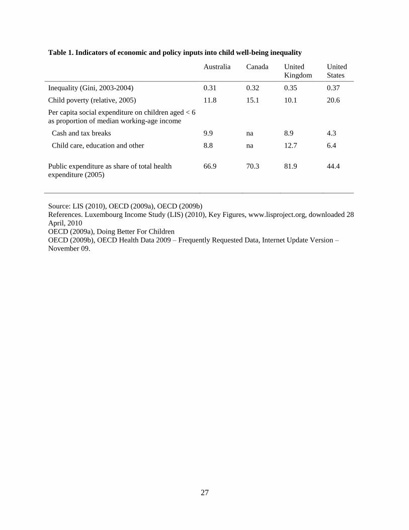
As shown in Table 1, each of these countries is characterized by levels of income inequality that
for the most part are above the OECD average — with Gini coefficients ranging from about 0.31 and 0.32
in Australia and Canada to 0.35 and 0.37 in the United Kingdom and the United States. They also differ
in their levels of social mobility in adult earnings across generations. The United States and United
Kingdom are identified as among the least mobile countries; Australia and Canada are among the most
mobile (Corak, 2006). The countries also differ in the levels of child poverty. Child poverty rates based
upon a relative income threshold (50% of median equivalised income) are as high as 21 percent in the
United States, but significantly lower at 15 percent in Canada, 12 per cent in Australia and 10 percent in
the United Kingdom.
Further, there are substantial differences in expenditures and policy frameworks for families with
young children, with the United States standing out as having the least generous provisions. Per capita
social expenditure on children younger than six years of age is significantly higher in Australia and the
United Kingdom than in the United States (Table 1).1 Moreover, across the four major domains of public
policy that affect families with young children – parental leave, child care, income supports, and health
insurance – the US has the weakest provisions, and if anything the gap between the US and the other
countries has widened in recent years as the other countries‘ policies to support families with young
children have evolved and expanded.
In Australia, one of the few countries to not offer paid parental leave (although it does offer 12
months of unpaid parental leave), plans are now underway to move to a system of 14 weeks of paid leave.
1 Expenditures in the US would be higher if they took into account tax support for employer-sponsored health
insurance.
4
Child care policies are evolving as well. Child care in Australia is provided by a combination of state,
non-governmental organization, and private providers. Historically there has been a split between ‗long
day care‘ (which is subsidised by the Federal government by providing child care rebates of up to 50% of
the fees) and ‗pre-school‘ (which is provided by the states as part of the education system). Payment for
preschool and availability differs from state to state, as does the school starting age. There is currently a
policy program initiated by the Council of Australian Governments (the Commonwealth and the States
acting together) to develop a unified early years framework that will bring together the Commonwealth
and State provisions and iron out the anomalies. Overall Australia is one of the lowest spenders in the
OECD on childhood services but in contrast provides relatively generous cash transfers to parents of
young children including a generous baby bonus, various family tax benefits and other in kind provisions.
The benefit system is also relatively progressive, with many of the cash transfers being targeted at the
most disadvantaged. Most Australians have access to comprehensive health care, which is mainly
publicly financed. The state provides financial incentives to doctors to encourage them to provide free
services to children under 16 and to income support recipients (Healy et al, 2006).
There were important expansions in family policy in Canada during the 1990s, with the cohort
studied here among the first to be exposed to some of these provisions. This includes the introduction of a
National Child Benefit and Early Childhood Development Agreements. These involved increased
financial transfers provided through the tax system targeted according to family income and the number
of children, and including supplements based on the number of children younger than seven years of age.
This change significantly increased the financial support to lower income families. At the same time there
was an increase of in-kind support through the development of early childhood learning and day care
facilities. These innovations also included an increase in paid parental leave through the unemployment
insurance program, so that beginning in 2001 up to one year of benefits are provided for a parent of a
newborn or adopted child. This includes 15 weeks of maternity benefits to the biological mother, and a
further 35 weeks of parental benefits that can be shared between the mother and the father. With regard to
health care, in Canada all children and their families are covered by a universal health care system. This
5
has been a longstanding program that permits families of all socio-economic backgrounds access to
publicly provided health care. In other domains there is also considerable variation in policies across the
ten provinces with, for example, Quebec offering essentially free child care for working mothers, and
Ontario currently implementing a program of full day kindergarten beginning at age four.
The past decade in the United Kingdom has witnessed dramatic expansions in programs and
supports for preschool age children (Waldfogel, 2010). Parents of the cohort studied here had the right to
take up to three months of unpaid parental leave, and mothers had the right to up to 29 weeks of job-
protected maternity leave, with 18 weeks paid (this has since been extended to a year of job-protected
maternity leave, with 9 months paid). In addition, low-income families with young children in this period
benefited from sizable increases in means-tested benefits as well as in the universal child allowance
program. Home visiting and child care services provided to children under age three by the Sure Start
program began on a small scale in 1999, just prior to the birth of this cohort, and expanded progressively
thereafter. And this cohort of children was the very first entitled to free universal preschool at age three
(although preschool for four year olds had been introduced six years earlier in 1998). As in Australia and
Canada, all children and their families benefit from universal health care, which is provided free at the
point of service by the National Health Service.
In contrast, the United States remains one of the few advanced industrialized countries without a
national policy providing a period of paid maternity leave (Waldfogel, 2006). Under the Family and
Medical Leave Act, qualifying employees may take up to 12 weeks of leave following a birth, but only
about half of new parents are covered and eligible, the period of leave is quite short by international
standards, and it is unpaid. The United States also differs from other advanced industrialized countries in
having a system of early childhood care and education that relies heavily on the private market. Subsidies
are provided to low-income working families, but there are not enough dollars to support all eligible
families. The federal Head Start program provides preschool to disadvantaged three and four year olds,
but, in spite of recent expansions, does not serve all eligible children. Public pre-kindergarten programs
serve only a small share (roughly one sixth) of the country‘s four year olds. Thus, a child‘s experience of
6
preschool remains very strongly correlated with parental resources, with the most advantaged children the
most likely to participate. Moreover, the US still does not provide universal health insurance coverage for
children and their families, even after the recent expansions in Medicaid and the Children‘s Health
Insurance Program, and the passage of health care reform in early 2010.
Whether these inputs have bearing on these outcomes is hard to tell without first documenting at
what point in the life cycle significant socio-economic gradients begin to emerge. A comparative analysis
may be helpful in appreciating the role of differences in public policy choices, but is obviously a
challenge because of the need for comparable data. Our analysis therefore takes advantage of rich data on
specific cohorts from each of the four countries to investigate variations in the connection between
parental resources and inequality in early child outcomes. Part of our contribution to the literature is,
therefore, methodological. We focus attention on measures and indicators that are relatively similar across
the very detailed surveys conducted in these countries, highlighting areas where future research and data
development in other countries might be directed.
The most important antecedent for our work is Waldfogel and Washbrook (2009, 2010) who
study income-related gaps in school readiness in the United States and the United Kingdom. Some of this
ground is covered by Corak, Curtis, and Phipps (2010) who study differences between Canada and the
United States, and by Bradbury and others on disparities in Australia (Bradbury, 2007; Katz and
Redmond, 2009; Redmond and Zhu, 2009).
While this work indicates that substantial gaps in school readiness exist in all four countries, only
two explicit cross-country comparisons have been carried out, and these focused only on pairs of
countries and examined different age groups and outcomes. Comparing income-related gaps in cognitive
and behavioral aspects of school readiness for preschool age children in the United States and the United
Kingdom, Waldfogel and Washbrook (2009, 2010) found that overall the results were quite similar. Large
gaps were evident in both countries between children in the bottom and middle income quintiles, and
between children in the top and middle income quintiles. Another point of agreement was that differences
in parenting behaviour were found to be an important mediator of the gaps in both countries. But some of
7
the findings in Corak et al. (2010) would suggest that these similarities are not likely to hold in general.
Their analysis of a range of cognitive, behavioral, and health outcomes for preschool and school age
children in Canada and the United States found that income-related gaps differed across the two countries.
In general, gaps in outcomes between low-income children and their more advantaged peers tended to be
larger in the US than they are in Canada, suggesting the presence of less mobility even in childhood.
3. The nature of the data and the measurement of outcomes and socio-economic background
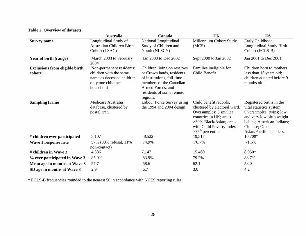
Our analysis is based upon: (1) the Longitudinal Study of Australian Children (LSAC), for Australia; (2)
the National Longitudinal Survey of Children and Youth (NLSCY), for Canada; (3) the Millennium
Cohort Study (MCS), for the UK; and (4) the Early Childhood Longitudinal Study-Birth Cohort (ECLS-
B), for the US. The UK and US studies each survey a single birth cohort, and we utilize both in their
entirety. The Australian and Canadian studies contain multiple birth cohorts from which we select the
sub-sets most comparable in time with the available UK and US data. Some details of the full scope of the
Australian and Canadian studies are given in the appendix; for the rest of the chapter we describe only
those cohorts used in the analysis.
These data are vast in both the breadth and depth of information they contain on children in all
stages of their lives. Indeed, some of these surveys could more accurately be described as containing
multiple surveys, involving separate questionnaires for parents, schools, and children. Our use of this
information is very selective, and driven by the objectives of our analysis and the need for cross-country
comparability. Table 2 provides an overview of some of the key features of each survey, with further
detail provided in the appendix. While the four datasets share many similarities the task of developing
comparable measures of outcomes and background is not simple.
We use information on more than 40,000 children across the four countries born in the first four
years of the 21st century. All these children were age 4 to 5 when their outcomes were assessed. The
samples were designed to be broadly representative of all children born in the country in the relevant time
window, and who remained resident until the dates of the follow-ups. Survey weights are used in all
8
analyses to adjust for over-sampling of certain groups, geographical clustering and non-random attrition.
The study-specific details on survey design are discussed in the appendix.
Each of the datasets contains three waves: Wave 1 when the children were age 0 or 1; Wave 2
when they were age 2 or 3; and Wave 3 when they were age 4 or 5. Each wave contains a Parent
Interview in which the most knowledgeable parent or care-giver—the child‘s biological mother in the
overwhelming majority of cases—responded to detailed questions on the family‘s socio-economic
circumstances and the early care environment of the child. The Wave 3 modules also include direct
assessments of the child‘s cognitive ability based on several well-known psychometric instruments,
parent reports of the frequency the child exhibited certain behaviors, and anthropomorphic
measurements.1 Hence comparable measures of both parental socio-economic status (―P‖) and cognitive,
socio-emotional and health outcomes in early childhood (―C1‖) can be constructed for all four countries.
The differences in child development age 4 or 5 are related to two indicators of parental
resources. Following the literature on the importance of parental education on child outcomes, the first
indicator we use is the highest educational qualification attained by the primary care-giver or partner who
is co-resident with the child at the time of the Wave 3 survey. We recode the information to UNESCO‘s
International Standard Classification of Education (ISCED), a scale explicitly designed to enable cross-
national comparisons. In this way it is possible to distinguish four common levels: lower secondary or
less (Level 2); upper secondary and post-secondary non-tertiary (Levels 3 and 4); first stage tertiary
practical/technical/occupationally-specific programs (Level 5B); and first stage tertiary theoretically-
based/research preparatory/highly skilled professional programs and second stage tertiary advanced
research qualifications (Levels 5A and 6).
Table A1 in the appendix provides details of common national qualifications that fall into each
category, and distributions of parental education for the full Wave 3 samples analyzed in this chapter.
Inspection of this table alerts us to the fact that the imposition of ISCED definitions results in apparently
very different education distributions across the countries. Although the proportion of families in the
lowest (Level 2) and highest (Levels 5A/6) categories are roughly similar in three of the four countries,
9
the Canadian distribution is heavily skewed toward the more highly educated. In addition, the proportions
of families falling into the middle two categories is complicated by the fact that Level 5B qualifications
are relatively more common in Canada and the United States, while Level 3/4 qualifications are the norm
among the ‗middle-educated‘ in Australia and the UK. We judge it likely that this discrepancy is more a
function of the rigidities of the ISCED classification system than evidence of higher average levels of
educational attainment in North America, and for this reason we group Levels 3, 4 and 5B together in a
single middle education category that covers around 50% of the population in three of the four countries
(and 40% in Canada). Our analysis uses this middle group as the reference category and documents the
difference in average outcomes between children in this group and those in the lowest and highest ISCED
categories.
Whether the difference in education distribution matters for our discussion of the correlation
between the distribution of P and C1 depends upon the mechanisms by which parental education acts on
outcomes. If parental education has a direct effect on outcomes, then it will be appropriate to compare
child outcomes within parental education groups. If, on the other hand, education acts as a mechanism for
sorting parents on the basis of academic aptitude, and it is this underlying aptitude that has an impact on
child outcomes, then a country which has a smaller proportion of the population in the extreme education
groups would be expected to have more unequal child outcomes across education groups. Because of the
possibility of this mechanism, some caution is required when comparing outcomes across education
groups.
The second indicator of parental socio-economic status is average gross household income,
divided into quintile groups in our main analysis (this is thus not subject to the issues raised in the
previous paragraph, but does assume that it is relative, rather than absolute, income which matters for
defining groups). We derive a measure of gross nominal household income at each of the three waves,
deflate to 2006 values using national price indices, and convert the amounts to US dollars using OECD
purchasing power parity indices (see appendix). The square root of household size is used as the
equivalence scale. These three observations of real gross equivalized household income for each family
10
are then averaged and the survey weights are used to define nationally-representative quintile boundaries.2
The intent of the averaging is to minimize the influence of transitory fluctuations in income due to
employment patterns after child birth, reporting or other factors that may introduce measurement error
into the analysis. Measurement error will have a tendency to lead to an understatement of the true
relationship between child outcomes and parental resources.
In addition it should be noted that the precision of the income questions posed in the parental
interviews differs across the countries. The least detailed measure comes from the US survey, in which
parents are asked to give their total gross annual household income in one of thirteen bands. We calculate
the percentage of US families in each band (separately for single-parent and couple families, and
separately for each wave), and use these percentiles to derive a comparable measure from the more
continuous income data in other countries. All families are then classified into one of 26 income/family
structure groups at each wave. A representative dollar value for gross household income is assigned to
each group and it is this ‗lumpy‘ nominal measure that is used in the rest of the income variable
derivation (see the appendix for further details of how these values are assigned).
We organize our analyses by two broad outcome domains: cognitive and socio-emotional. For
each domain, we focus primarily on a single outcome measure that is the most comparable across the full
set of four countries. We then go on to explore other outcomes that are measured consistently in fewer
than four countries or that measure a more narrow sub-set of skills, but which provide some evidence on
the robustness of our core findings (see the appendix for details of these additional outcomes). Our focal
cognitive outcomes are picture vocabulary test scores. Children‘s receptive vocabulary is measured in the
Australian, Canadian and American datasets with items from the Peabody Picture Vocabulary Test
(PPVT). In this assessment the child is shown pictures on an easel and is asked to identify the picture that
best represents the meaning of the word read out by the interviewer.3 The UK picture vocabulary
assessment—the British Ability Scales Naming Vocabulary (BAS-NV) test—differs slightly from the
PPVT by requiring the child to name out loud the object shown in a single picture. Although this assesses
expressive rather than receptive vocabulary, both the BAS-NV and the PPVT are well-known assessments
11
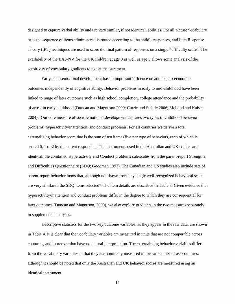
designed to capture verbal ability and tap very similar, if not identical, abilities. For all picture vocabulary
tests the sequence of items administered is routed according to the child‘s responses, and Item Response
Theory (IRT) techniques are used to score the final pattern of responses on a single ―difficulty scale‖. The
availability of the BAS-NV for the UK children at age 3 as well as age 5 allows some analysis of the
sensitivity of vocabulary gradients to age at measurement.
Early socio-emotional development has an important influence on adult socio-economic
outcomes independently of cognitive ability. Behavior problems in early to mid-childhood have been
linked to range of later outcomes such as high school completion, college attendance and the probability
of arrest in early adulthood (Duncan and Magnuson 2009; Currie and Stabile 2006; McLeod and Kaiser
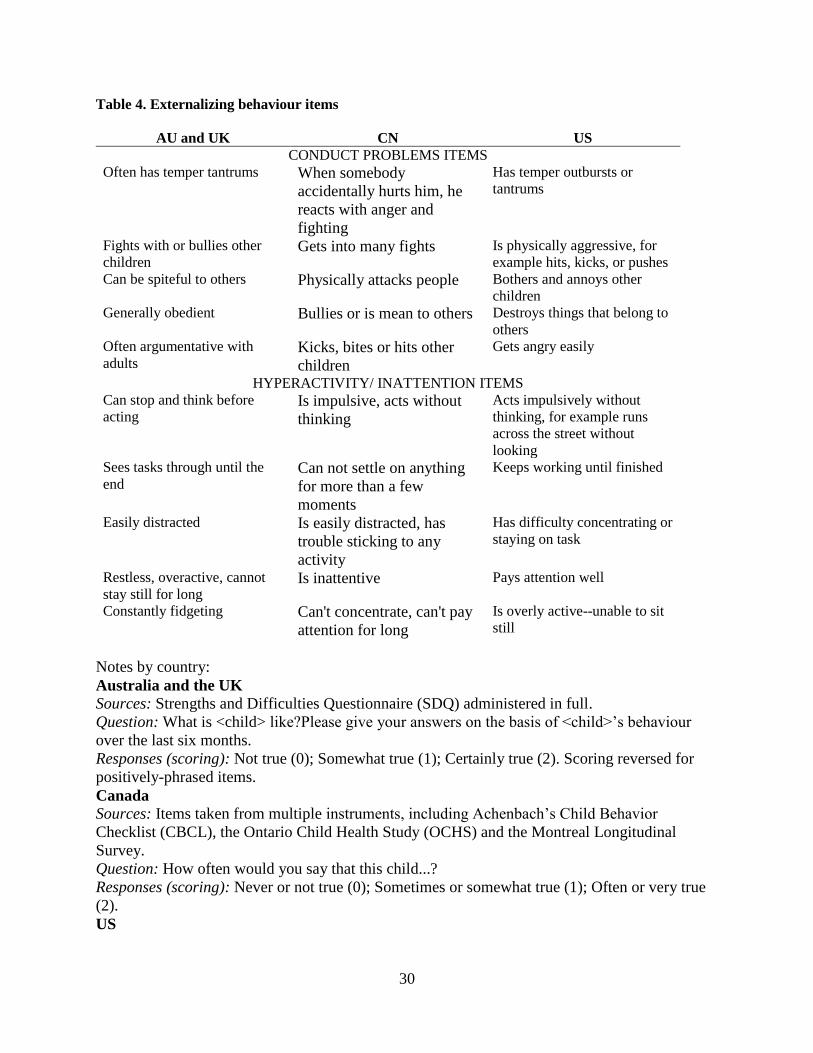
2004). Our core measure of socio-emotional development captures two types of childhood behavior
problems: hyperactivity/inattention, and conduct problems. For all countries we derive a total
externalizing behavior score that is the sum of ten items (five per type of behavior), each of which is
scored 0, 1 or 2 by the parent respondent. The instruments used in the Australian and UK studies are
identical: the combined Hyperactivity and Conduct problems sub-scales from the parent-report Strengths
and Difficulties Questionnaire (SDQ; Goodman 1997). The Canadian and US studies also include sets of
parent-report behavior items that, although not drawn from any single well-recognized behavioral scale,
are very similar to the SDQ items selected4. The item details are described in Table 3. Given evidence that
hyperactivity/inattention and conduct problems differ in the degree to which they are consequential for
later outcomes (Duncan and Magnuson, 2009), we also explore gradients in the two measures separately
in supplemental analyses.
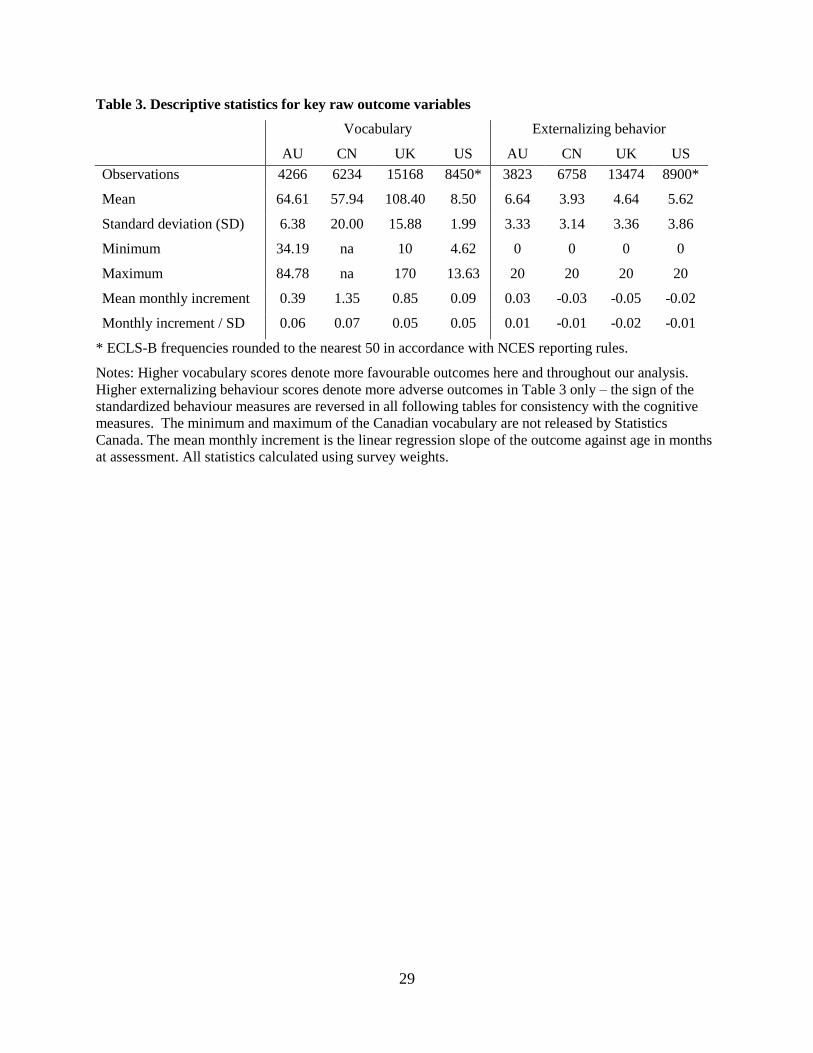
Descriptive statistics for the two key outcome variables, as they appear in the raw data, are shown
in Table 4. It is clear that the vocabulary variables are measured in units that are not comparable across
countries, and moreover that have no natural interpretation. The externalizing behavior variables differ
from the vocabulary variables in that they are nominally measured in the same units across countries,
although it should be noted that only the Australian and UK behavior scores are measured using an
identical instrument.
12
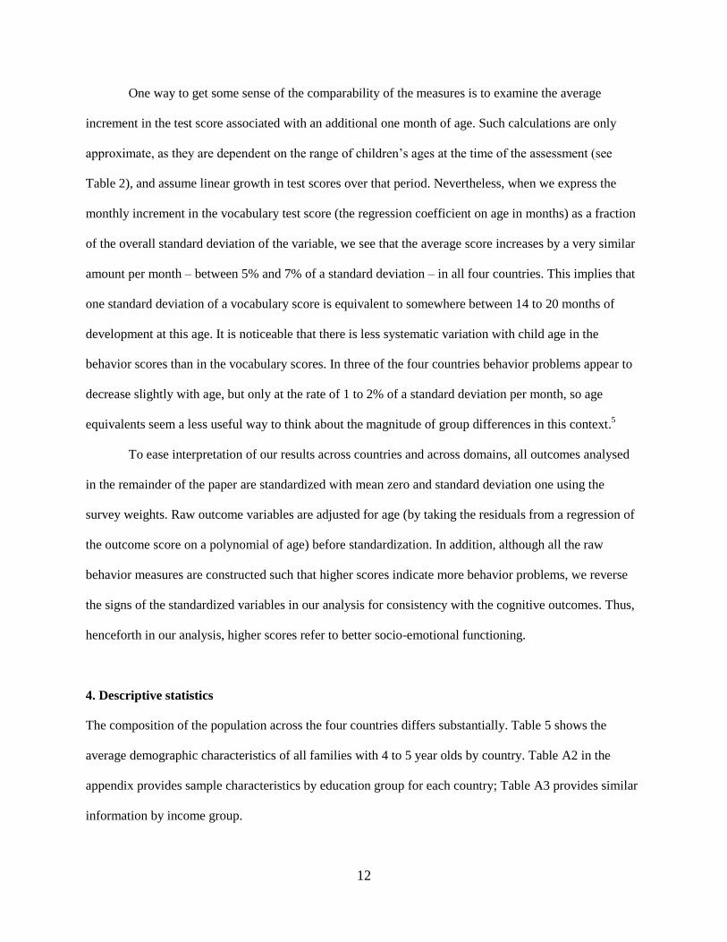
One way to get some sense of the comparability of the measures is to examine the average
increment in the test score associated with an additional one month of age. Such calculations are only
approximate, as they are dependent on the range of children‘s ages at the time of the assessment (see
Table 2), and assume linear growth in test scores over that period. Nevertheless, when we express the
monthly increment in the vocabulary test score (the regression coefficient on age in months) as a fraction
of the overall standard deviation of the variable, we see that the average score increases by a very similar
amount per month – between 5% and 7% of a standard deviation – in all four countries. This implies that
one standard deviation of a vocabulary score is equivalent to somewhere between 14 to 20 months of
development at this age. It is noticeable that there is less systematic variation with child age in the
behavior scores than in the vocabulary scores. In three of the four countries behavior problems appear to
decrease slightly with age, but only at the rate of 1 to 2% of a standard deviation per month, so age
equivalents seem a less useful way to think about the magnitude of group differences in this context.5
To ease interpretation of our results across countries and across domains, all outcomes analysed
in the remainder of the paper are standardized with mean zero and standard deviation one using the
survey weights. Raw outcome variables are adjusted for age (by taking the residuals from a regression of
the outcome score on a polynomial of age) before standardization. In addition, although all the raw
behavior measures are constructed such that higher scores indicate more behavior problems, we reverse
the signs of the standardized variables in our analysis for consistency with the cognitive outcomes. Thus,
henceforth in our analysis, higher scores refer to better socio-emotional functioning.
4. Descriptive statistics
The composition of the population across the four countries differs substantially. Table 5 shows the
average demographic characteristics of all families with 4 to 5 year olds by country. Table A2 in the
appendix provides sample characteristics by education group for each country; Table A3 provides similar
information by income group.
13
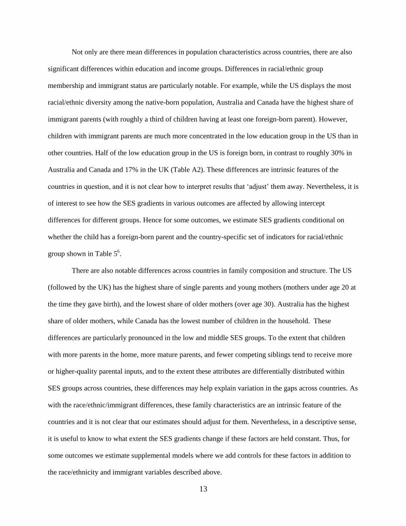
Not only are there mean differences in population characteristics across countries, there are also
significant differences within education and income groups. Differences in racial/ethnic group
membership and immigrant status are particularly notable. For example, while the US displays the most
racial/ethnic diversity among the native-born population, Australia and Canada have the highest share of
immigrant parents (with roughly a third of children having at least one foreign-born parent). However,
children with immigrant parents are much more concentrated in the low education group in the US than in
other countries. Half of the low education group in the US is foreign born, in contrast to roughly 30% in
Australia and Canada and 17% in the UK (Table A2). These differences are intrinsic features of the
countries in question, and it is not clear how to interpret results that ‗adjust‘ them away. Nevertheless, it is
of interest to see how the SES gradients in various outcomes are affected by allowing intercept
differences for different groups. Hence for some outcomes, we estimate SES gradients conditional on
whether the child has a foreign-born parent and the country-specific set of indicators for racial/ethnic
group shown in Table 56.
There are also notable differences across countries in family composition and structure. The US
(followed by the UK) has the highest share of single parents and young mothers (mothers under age 20 at
the time they gave birth), and the lowest share of older mothers (over age 30). Australia has the highest
share of older mothers, while Canada has the lowest number of children in the household. These
differences are particularly pronounced in the low and middle SES groups. To the extent that children
with more parents in the home, more mature parents, and fewer competing siblings tend to receive more
or higher-quality parental inputs, and to the extent these attributes are differentially distributed within
SES groups across countries, these differences may help explain variation in the gaps across countries. As
with the race/ethnic/immigrant differences, these family characteristics are an intrinsic feature of the
countries and it is not clear that our estimates should adjust for them. Nevertheless, in a descriptive sense,
it is useful to know to what extent the SES gradients change if these factors are held constant. Thus, for
some outcomes we estimate supplemental models where we add controls for these factors in addition to
the race/ethnicity and immigrant variables described above.
14
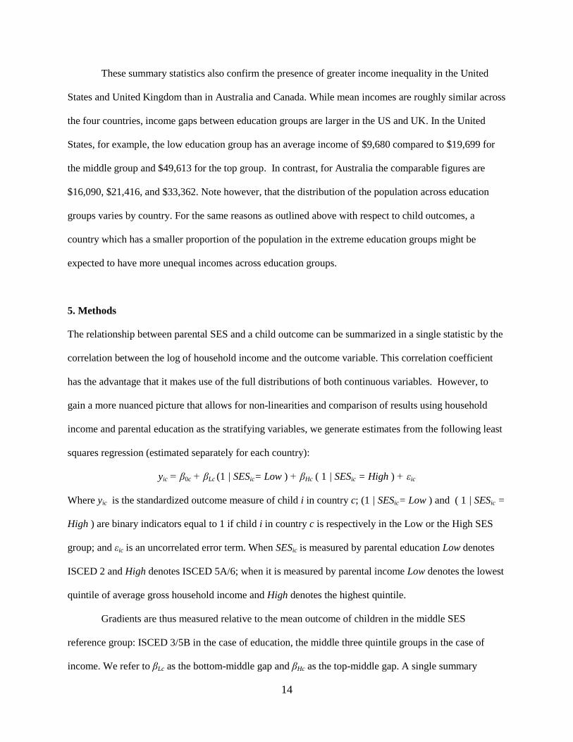
These summary statistics also confirm the presence of greater income inequality in the United
States and United Kingdom than in Australia and Canada. While mean incomes are roughly similar across
the four countries, income gaps between education groups are larger in the US and UK. In the United
States, for example, the low education group has an average income of $9,680 compared to $19,699 for
the middle group and $49,613 for the top group. In contrast, for Australia the comparable figures are
$16,090, $21,416, and $33,362. Note however, that the distribution of the population across education
groups varies by country. For the same reasons as outlined above with respect to child outcomes, a
country which has a smaller proportion of the population in the extreme education groups might be
expected to have more unequal incomes across education groups.
5. Methods
The relationship between parental SES and a child outcome can be summarized in a single statistic by the
correlation between the log of household income and the outcome variable. This correlation coefficient
has the advantage that it makes use of the full distributions of both continuous variables. However, to
gain a more nuanced picture that allows for non-linearities and comparison of results using household
income and parental education as the stratifying variables, we generate estimates from the following least
squares regression (estimated separately for each country):
yic = β0c + βLc (1 | SESic= Low ) + βHc ( 1 | SESic = High ) + εic
Where yic is the standardized outcome measure of child i in country c; (1 | SESic= Low ) and ( 1 | SESic =
High ) are binary indicators equal to 1 if child i in country c is respectively in the Low or the High SES
group; and εic is an uncorrelated error term. When SESic is measured by parental education Low denotes
ISCED 2 and High denotes ISCED 5A/6; when it is measured by parental income Low denotes the lowest
quintile of average gross household income and High denotes the highest quintile.
Gradients are thus measured relative to the mean outcome of children in the middle SES
reference group: ISCED 3/5B in the case of education, the middle three quintile groups in the case of
income. We refer to βLc as the bottom-middle gap and βHc as the top-middle gap. A single summary
15
measure of the inequality in child outcomes is given by ( βLc - βHc ), the difference in mean outcomes
between those in the high and low SES groups. All outcome variables are standardized to have unit
variance, and so these coefficients represent the number of standard deviations difference between the
different SES groups. The appropriate survey weights are used in the calculation of all estimates and
sample design features are accounted for in the calculation of confidence intervals.7
All four of these countries are characterized by diversity in terms of ethnic and racial identity and
immigrant status. For this reason we augment the above equation with controls for race, ethnicity, and
immigrant status to examine the extent to which SES gradients are associated with demographic
heterogeneity.8 It is often suggested in the literature that race and ethnicity play a particularly important
role in distinguishing child outcomes in the United States from other countries. But we should also note
that these countries have very different policies with respect to immigration selection rules. The variables
used to define race and ethnicity are, of necessity, different in each country (see Table 5), but we believe
that we have been able to capture the most salient features of the within-country heterogeneity.
As discussed, a second way in which families differ across countries, and that might matter in
explaining differential SES gaps, is their structure and composition. Accordingly, we estimate an
additional model in which we further add controls for single parenthood, age of mother, and number of
children in the household.
6. Results
Figure 1 displays the correlations between log gross household income and our two focal outcomes, with
95% confidence intervals shown by the range plots. On the basis of this simple statistic, the four countries
appear to divide into two groups of two – Australia and Canada show similar relationships between
family income and child outcomes that are markedly weaker than the correlations for the United Kingdom
and the United States. In both cases the Canadian correlation is the lowest of the four, closely followed by
Australia. Among the high correlations, the US income-vocabulary relationship is slightly stronger than
that in the UK, while the reverse is true for the income-externalizing behavior relationship.
16
However, while these correlations tell us about the overall strength of the association between
parental SES and child outcomes, they do not tell us where in the distribution this occurs. For this reason,
we turn next to models that explicitly compare outcomes for the top group and the middle, and for the
bottom group and the middle.
Figure 2 explores the associations of SES and vocabulary outcomes in more detail. Panel A refers
to the overall country results with no controls for demographic characteristics, Panel B shows the results
after adding controls on racial/ethnic/immigrant composition, and Panel C adds further controls for family
composition and mother‘s age at birth. The lighter bars in these figures show βHc , the mean outcome
score for the ‗top‘ group minus the mean score for the ‗middle‘ group. The darker bars similarly show βLc,
the bottom-middle gap, with the combined bar lengths ( βLc - βHc ), the gap between the top and bottom,
summarized in parentheses alongside the relevant bars. The outcomes are all standardised measures, so
that a difference of 0.50 represents a half standard deviation difference in outcomes. The figures also
show approximate 95 per cent confidence intervals. Note that countries can be significantly different from
one another even if the confidence intervals overlap to some extent. Details of all estimates, along with
pairwise t-tests of country differences, are provided in the appendix.
Focusing first on the unconditional estimates in Panel A, we see that the overall differences in
vocabulary scores between the top and bottom SES groups mimic the pattern of correlations shown in
Figure 2, regardless of whether parental income or education is used as the SES indicator. The US shows
the greatest disparities, followed by the UK and Australia, with the smallest average differences found in
Canada. Pairwise t-tests of cross-country differences confirm that the top-bottom US gradient is
significantly larger than those of each of the other three countries, and also that this gradient is
significantly smaller in Canada than the UK. However, we cannot reject the hypotheses of no significant
differences between Australia and either Canada or the UK.
Comparison of the top-middle and bottom-middle gaps reveals that these country differences are
almost entirely driven by variation at the upper part of the SES distribution. In no case is the bottom-
middle income-related gap significantly different between any pair of countries, although children from
17
the lowest educated families in Canada (6.2% of the cohort) do perform significantly better in a relative
sense than their counterparts in either the UK or the US.
Differences at the top end of the distribution are much more marked. American children in the
highest education households score 0.60 of a standard deviation higher than children from the middle
education group, compared to 0.43 for the UK and 0.33 to 0.35 for the other two countries. A similar
pattern is seen for income, with American children in the highest income households scoring 0.62 of a
standard deviation higher than children from the middle income group. This gap ranges from to 0.25
(Canada) to 0.33 (Australia) to 0.43 (UK) in the other countries. Again, we cannot reject the hypothesis
that the top-middle gaps are equal in Australia and Canada on either measure, nor that the top-middle
income gap is the same in Australia and the UK. Other than this, all country differences in the top-middle
gaps, and in particular the differences between the US and all other countries, are significant.
Panel B displays a similar set of results, but based upon models that include controls for
racial/ethnic diversity and immigrant status.9 The contrast between these results and those in Panel A
highlights the extent to which SES gradients are associated with this heterogeneity, and in particular the
extent to which the greater divergence in vocabulary scores in the United States is associated with the
racial and ethnic heterogeneity in that country.
As expected, the overall lengths of the bars are generally either smaller or the same length as
those in Panel A (this can also be seen in appendix Table A4). The portion of the SES gradients explained
by these controls is particularly large for the US. For example, after controlling for race/ethnicity and
immigration status, the gap in vocabulary scores between children of middle-income and high-income
parents falls by 36% in the US as compared to 9% in Australia and 24% in the UK. After controlling for
race/ethnicity and immigration status the top-middle differences between the US and both Canada and
Australia are reduced, but not eliminated. No significant differences in the any of the vocabulary
gradients between the US and the UK, however, remain in Panel B. It appears that some, but not all, of
the greater variation in vocabulary outcomes in the US is associated with the divergent outcomes of
18
children in different racial/ethnic and nativity groups within that country, but that significant differences
between the US and other countries remain.
Panel C shows the estimates from a further set of models adding, in addition to the above
controls, a set of controls for single parent, age of mother (binary indicators for below 20 or above 30 at
the time of the birth, with age 20 to 30 as the reference category), and number of children in the home.
The results show that the correlation between family composition and SES contributes to the vocabulary
gradients in all four countries, but does little to explain the country differences, which remain largely
unchanged from Panel B. Again, no differences between the US and the UK remain, but high SES
children in the US continue to exhibit an advantage in vocabulary that is relatively greater than for their
counterparts in either Australia or Canada.
While the vocabulary measures presented in Figure 2 are the most comparable measures of child
cognitive development across the four countries, the surveys also include a number of other cognitive
scores. Figure 3 offers a brief look at the two cognitive domains where we have comparable data for three
countries (estimates of the unconditional gradients in all supplementary outcomes are available in the
appendix). It is unfortunate that the instruments used to measure math skills differ considerably across the
three countries in which they were included, and are only available for the UK at the earlier Wave 2 (age
3). The copying instrument was identical in the Australian and Canadian surveys, but again differs in the
US case. Hence we cannot draw strong conclusions from the correlations shown in Figure 3, but it is
noticeable that the ranking of the countries under both additional measures is the same as for the
vocabulary measure – the US shows the greatest disparities in both outcomes, followed by the UK and
Australia, with the lowest correlations found in the Canadian measures. Analysis of the top-middle and
bottom-middle gaps (not shown here) shows that as before higher US gradients are generally driven by
greater disparities at the top of the SES distribution, although some differences in the relative position of
the lowest SES groups are also discernable.
Figure 4 depicts in more detail the socio-economic gradients in our most comparable measure of
socio-emotional functioning, externalizing behaviors. As suggested by the correlations in Figure 1, SES-
19
related disparities in behavioral outcomes are smaller than in cognitive outcomes in all countries. The
unconditional results in Panel A highlight Canada as a clear outlier in this domain, and t-tests provided in
the appendix confirm that all top-bottom and top-middle gradients – whether by income or education –
are significantly smaller in Canada than all the other three countries. Assessment of the relative position
of low SES children in Canada varies depending on whether income or education is the stratifying
variable – the bottom-middle income gap is not significantly different in Canada to that in any of the other
countries, but children of the low-educated show smaller disparities in externalizing behavior than
elsewhere.
In contrast to the results for vocabulary outcomes, the greatest disparities in behavioral outcomes
are found not in the US but in the UK. Differences between high- and middle-SES children are virtually
identical in the two countries, and it is solely the relatively greater level of behavioral problems of low
SES children in the UK that is responsible for this finding.
The addition of racial/ethnic/nativity controls in Panel B makes very little difference to the
estimated gradients in any country, but the demographic controls added in Panel C have a stronger
explanatory role, suggesting that somewhat different mechanisms underlie the gradients in cognitive and
socio-emotional outcomes. The smaller behavioral gradients in Canada are not accounted for by any of
the controls, but differences between the UK and both the US and Australia become insignificant when
family composition and maternal age are held constant. Additional analyses provided in the appendix find
little systematic variation across countries in the gradients of the sub-domains of hyperactivity/inattention
and conduct problems. Low SES children in the UK have the greatest disparities in both sub-domains of
all the four countries, and overall gradients are the lowest in Canada on both measures.
7. Some implications
While it is very difficult to ascribe the variation in outcomes to particular policies or institutions, our
results do complement other indicators of social inequality and mobility, and offer a starting point to
reflect upon the particular accomplishments and challenges in each country. In particular, our results
20
indicate that, in spite of the broad similarities, young children grow up in very different contexts in these
four countries.
The descriptive statistics in Table 5 highlight the fact that the resources—both monetary and non-
monetary—families are able to bring to bear differ in an absolute sense across these countries. While
overall average income, at about $26,000 to $29,000, is about the same it is distributed differently, with
lower educated parents having substantially less income in the United Kingdom, and particularly in the
United States. But this reflects a number of other demographic factors that also determine the amount of
time and other non-monetary resources parents have to invest in their young children. Children raised in
the bottom of the income distribution are more likely to have parents with low levels of education,
mothers who tend to be younger at the child‘s birth, and more likely to be in a single parent household.
Racial/ethnic and cultural diversity also play out across socio-economic groups in a different way in the
four countries. Australia and Canada have high proportions of children living with foreign-born parents,
who are equally as likely to be found among low-income as among high-income groups. The United
Kingdom has a lower proportion of second-generation immigrant children in general but again there is
little relation with socio-economic status, while in the United States the high proportion of children with
foreign-born parents is concentrated disproportionately in the lower socio-economic groups.
The extent of the disparities and differences across these countries is somewhat muted when
account is taken of the diversity in demographic composition of the population. The outcomes look more
similar when account is made of these differences, particularly between the US and UK where no
significant differences remain. The characteristics of families in different socio-economic groups clearly
have an impact on social outcomes of the next generation, and like many other countries in the OECD
these countries will increasingly face the need to cope with racial and ethnic diversity and other
demographic shifts, and to integrate and foster the development of new citizens. But there are also a host
of broader issues associated with the support that families in challenging circumstances can rely upon. As
we emphasized earlier, children experience very different policy contexts across the four countries in four
policy domains that determine the amount of time parents have for non-market activities associated with
21
family life, as well as other material resources important for the development of children: parental leave,
child care, income supports for families with young children, and health insurance. Such policies may be
one dimension contributing to a much more muted socio-economic gradient with respect to externalizing
behaviors in Canada. Exploring the role of these policy contexts in early inequalities is an important
challenge for future research.
8. Conclusion
This chapter is intended to shed light on the origins of inequality and social immobility by examining the
gaps that exist in cognitive and socio-emotional development in early childhood in four countries that
share a good deal in common, but that also display important differences. We emphasize three basic
findings and also offer some thoughts about the use of cross-country comparative data.
First, our analysis of four and five year olds in Australia, Canada, the United Kingdom, and the
United States finds that while gaps in readiness to learn between the children of relatively advantaged and
relatively disadvantaged families are clearly evident in each country, there is also variation across them.
Disparities in Australia and Canada are consistently smaller on a range of outcome measures than
disparities in the US and the UK.
Second, differences in cognitive development seem to be more strongly linked to disparities in
parental resources in the United States than in the other countries, with the difference driven by a
particularly large advantage of high-SES children relative to those in the middle. Thus, any explanation
of cross-national differences must account both for why children at the top out-perform children in the
middle to different degrees. One hypothesis, which might be tested in future research, is that families in
the middle receive less support in the US due to the highly targeted nature of its social welfare system,
and thus lag further behind those at the top. While the very poorest in the US are eligible for programs
such as Medicaid and Head Start, these benefits are withdrawn at a much lower level of income in the US
than in countries such as Canada and the UK. High rates of full-time maternal employment, combined
with a largely private child care market in which quality is very costly, is another factor that may
22
disadvantage middle-income children in the US relative to those in other countries. Another possible
factor is the greater disparity of incomes in the US, with particularly high incomes for those at the top.
Third, the cross-country pattern of SES disparities in school readiness differs depending on the
outcome measure considered. Social and behavioral development is less strongly linked than cognitive
development to family background in all countries. In comparative terms, low SES children in the UK
have high levels of behavior problems but appear in line with other countries in terms of their deficits in
cognitive outcomes. Conversely, the cognitive advantages displayed by high SES children in the US are
not accompanied by unusually low levels of behavior problems relative to other countries.
In addition to these substantive conclusions, we also offer a call for more attention to comparable
data across a larger number of OECD countries. Our analysis is descriptive, but good description is the
first step to informed policy discussion and hypotheses about causal relationships. While the data we rely
upon are extremely rich, they are designed to inform public policy by offering a longitudinal perspective
on child development in a particular national context. This no doubt is central to an appreciation of the
causal mechanisms determining outcomes, but without attention to the comparability of measures across
countries, an opportunity is missed to illustrate the role of different public policies and social situations.
We draw an analogy to the important role that the Programme of International Student Assessment has
had on discussions of schooling outcomes for 15 year olds across the entire OECD. Now that public
policy has come to fully appreciate that this variation is also rooted in disparities of outcomes during the
early years, the development of a similar instrument offering comparable cross-sectional indicators over
many more countries than we are able to examine here would inform the quality of future research and
public discourse directed to the well being of children.
In this paper we find clear evidence of differences in the correlation between socio-economic
status and child cognitive outcomes. This correlation is strongest in the US and the UK and weakest in
Australia and Canada. Although our four countries share a common heritage, their economic and social
policy environments differ in many ways. Although our results cannot be used to point unambiguously to
23
any particular causal determinant, they do suggest the importance of future research on the role that
specific policies might play.
Our findings are also relevant to some of the larger questions about intergenerational mobility
addressed in this volume. Previous research has shown a noticeable (though admittedly not large) positive
correlation between high parental inequality and high levels of parent-child immobility of adult income
levels (Bjorklund and Jantti 2008; Corak 2006). Indeed the US experience of high inequality and high
intergenerational immobility is a key data point for this cross-national correlation. It is certainly not
inevitable that high inequality should imply low mobility, indeed the rhetoric advanced in unequal
societies is often just the opposite. The results found here can be seen as contributing to an explanation of
this relationship. The distribution of resources available to families with young children does seem to
matter for their developmental outcomes – and this in turn is one part of the explanation for the broader
patterns of intergenerational mobility.
24
Endnotes
1 In some cases assessments at Wave 2 are also available. We make only limited use of these measures for
comparability reasons, and make it clear when we do so that the outcome in question is not taken from the default
Wave 3 survey. 2 We use measures from one or two waves if information on all three waves is not available.
3 It should be noted, however, that different items and versions of the PPVT were used in different countries. These
details are available in the appendix. 4 We are confident that although the wording of items is different across countries, collectively they capture similar
emotional and behavioral concepts. A number of alternative scales are commonly used to measure child behaviour
problems. Two of the most widely used – the Rutter scale and the Child Behavior Checklist – have both been shown
to predict high-psychiatric-risk cases with the same accuracy as the SDQ (Goodman 1997; Goodman and Scott
1999). In addition, note that differences in distribution of responses to items that vary across countries will only
affect our conclusions to the extent that they differ systematically with socio-economic status. 5 The pattern of decreasing behavior problems with age is supported by a comparison of the UK scores at Wave 2
(age 3) and Wave 3 (age 5) as the mean falls from 6.46 to 4.64 over this period. 6 Note that the Australian survey does not record the child‘s racial/ethnic background as such, so we are able only to
distinguish between Indigenous children and the rest. Definitions from the Canadian survey relate to the
race/ethnicity of the main carer rather than the child. 7 The exception to this is that the confidence intervals for the correlation coefficient in Australia do not take account
of sample design. Also, in all countries, our confidence intervals do not account for the sampling variance associated
with the standardization of the dependent variables, and so are slightly too narrow. 8 An alternative approach would be to re-estimate our models on a sub-sample consisting only of children with non-
minority native-born parents. We estimated such models as a robustness check, as discussed below. 9 An alternative approach would be to estimate a model only for the non-minority and native-born sub-group in each
country. We did estimate such models as a robustness check (shown in appendix table A3) and found the results
were broadly comparable to those obtained in the full sample model with controls for minority status and foreign-
born. We also estimated more detailed models including controls for language spoken in the home (although the
variables regarding language are not fully comparable across countries) and results were similar.
25
References
Almond, Douglas and Janet Currie. 2010. ―Human Capital Development Before Age Five.‖ NBER
Working Paper 15827. Cambridge, MA.
Bradbury, Bruce. 2007. "Child Outcomes and Family Socio-Economic Characteristics." SPRC Report
9/07, prepared for the Department of Families, Community Services and Indigenous Affairs.
Carneiro, Pedro and James Heckman. 2003. ―Human Capital Policy.‖ In James Heckman, Alan Krueger,
and Benjamin Friedman (eds). Inequality in America: What Role for Human Capital Policies?
Cambridge, MA: MIT Press.
Case, Anne and Christina Paxson. 2010. ―Causes and Consequences of Early Life Health.‖ NBER
Working Paper 15637. Cambridge, MA.
Corak, Miles. 2006. ―Do Poor Children Become Poor Adults? Lessons for Public Policy from a Cross
Country Comparison of Generational Earnings Mobility.‖ In John Creedy and Guyonne Kalb (eds).
Research on Economic Inequality. Amsterdam: Elsevier Press.
Corak, Miles (2008). Immigration in the Long Run: The Education and Earnings Mobility of Second-
Generation Canadians. Institute for Research on Public Policy Choices. Volume 14, no. 13.
Corak, Miles, Lori Curtis, and Shelley Phipps. 2010. ―Economic Mobility, Family Background, and the
Well-Being of Children in the United States and Canada.‖ Revised version of a paper presented at a
conference on Intergenerational Mobility Within and Across Nations, University of Wisconsin-
Madison, September 2009.
Cunha, Flavio, James Heckman, Lance Lochner, and Dmitri Masterov. (2005) Interpreting the evidence
on life cycle skill formation. In Eric Hanushek and Finis Welch (eds.) Handbook of the Economics
of Education. Amsterdam: North Holland.
Currie, Janet. 2009. ―Healthy, Wealthy, and Wise: Socioeconomic Status, Poor Health in Childhood, and
Human Capital Development.‖ Journal of Economic Literature 47(1): 87-122.
Currie, Janet and Mark Stabile. 2006. ―Child Mental Health and Human Capital Accumulation: The Case
of ADHD.‖ Journal of Health Economics 25(6): 1094-1118.
De Lemos, Molly (2002). ―Patterns of Young Children‘s Development: An International Comparison of
Development as Assessed by Who Am I?‖. Research Paper R-02-5E. Applied Research Branch,
Strategic Policy, Human Resources Development Canada.
Duncan, Greg and Katherine Magnuson. 2009. ―The Nature and Impact of Early Achievement Skills,
Attention and Behavior Problems.‖ Paper presented at the conference on “Rethinking the Role of
Neighborhoods and Families on Schools and School Outcomes for American Children,‖ November
19-20, 2009, Washington, DC.
Esping-Anderson, Gosta. 1990. Three Worlds of Welfare Capitalism. Princeton, NJ: Princeton University
Press.
26
Esping-Anderson, Gosta. 2005. ―Social Inheritance and Equal Opportunities Policies.‖ In Simone
Delorenzi, Jodie Reed and Peter Robinson (eds.) Maintaining Momentum: Promoting Social
Mobility and Life Chances from Early Years to Adulthood. London: Institute for Public Policy
Research.
Goodman R (1997) ―The Strengths and Difficulties Questionnaire: A Research Note.‖ Journal of Child
Psychology and Psychiatry, 38, 581-586.
Goodman R, and Stephen Scott (1999) ―Comparing the Strengths and Difficulties Questionnaire and the
Child Behavior Checklist: Is Small Beautiful?.‖ Journal of Abnormal Child Psychology, 27(1), 17-
24.
Healy Judith, Sharman Evelyn, Lokuge Buddhima 2006. Australia: Health system review. Health Systems
in Transition 2006; 8(5): 1–158.
Heckman, James J., and Lance Lochner. 2000. ―Rethinking Education and Training Policy:
Understanding the Sources of Skill Formation in a Modern Economy.‖ In Sheldon Danziger and
Jane Waldfogel (eds). Securing the Future: Investing in Children from Birth to College. New York:
Russell Sage Foundation.
Katz, I. and Redmond, G.. 2009. ―Family Income as a Protective Factor for Child Outcomes.‖ In K.
Rummery, I. Greener and C. Holden (eds.), Social Policy Review 21, The Policy Press, Bristol.
Knudsen, Eric I., James J. Heckman, Judy L. Cameron, and Jack P. Shonkoff (2006). ―Economic,
neurobiological, and behavioural perspectives on building America‘s future workforce.‖
Proceedings of the National Academy of Sciences. Vol. 103, No. 27 pp. 10155-10162.
McLeod, Jane D. and Karen Kaiser (2004). ―Child Emotional and Behavioral Problems in Educational
Attainment.‖ American Sociological Review. Vol. 69, No. 5 pp. 636-658.
OECD (2006). Where Immigrant Children Succeed: A Comparative Review of Performance and
Engagement in PISA 2003. Paris: OECD.
Redmond, G. and Zhu, A. 2009. ―Maternity Leave and Child Outcomes.‖ Final Report for Department of
Families, Housing, Community Services and Indigenous Affairs December 2009, Social Policy
Research Centre, The University of New South Wales,
Smith, James. 2009. ―The Impact of Childhood Health on Adult Labor Market Outcomes.‖ The Review of
Economics and Statistics 91(3): 478-489.
Waldfogel, Jane (2006). What Children Need. Cambridge: Harvard University Press.
Waldfogel, Jane (2010). Britain’s War on Poverty. New York: Russell Sage Foundation.
Waldfogel, Jane and Elizabeth Washbrook (2009). Early Years Policy. Report for the Sutton Trust.
Waldfogel, Jane and Elizabeth Washbrook (2010). ―Income-Related Gaps in School Readiness in the US
and UK.‖ Revised version of a paper presented at a conference on Intergenerational Mobility
Within and Across Nations, University of Wisconsin-Madison, September 2009.
27
Table 1. Indicators of economic and policy inputs into child well-being inequality
Australia Canada United
Kingdom
United
States
Inequality (Gini, 2003-2004) 0.31 0.32 0.35 0.37
Child poverty (relative, 2005) 11.8 15.1 10.1 20.6
Per capita social expenditure on children aged < 6
as proportion of median working-age income
Cash and tax breaks 9.9 na 8.9 4.3
Child care, education and other 8.8 na
12.7 6.4
Public expenditure as share of total health
expenditure (2005)
66.9 70.3 81.9 44.4
Source: LIS (2010), OECD (2009a), OECD (2009b)
References. Luxembourg Income Study (LIS) (2010), Key Figures, www.lisproject.org, downloaded 28
April, 2010
OECD (2009a), Doing Better For Children
OECD (2009b), OECD Health Data 2009 – Frequently Requested Data, Internet Update Version –
November 09.
28
Table 2. Overview of datasets
Australia Canada UK US
Survey name Longitudinal Study of
Australian Children Birth
Cohort (LSAC)
National Longitudinal
Study of Children and
Youth (NLSCY)
Millennium Cohort Study
(MCS)
Early Childhood
Longitudinal Study Birth
Cohort (ECLS-B)
Year of birth (range) March 2003 to February
2004
Jan 2000 to Dec 2002 Sept 2000 to Jan 2002 Jan 2001 to Dec 2001
Exclusions from eligible birth
cohort
Non-permanent residents;
children with the same
name as deceased children;
only one child per
household
Children living on reserves
or Crown lands, residents
of institutions, full-time
members of the Canadian
Armed Forces, and
residents of some remote
regions.
Families ineligible for
Child Benefit
Children born to mothers
less than 15 years old;
children adopted before 9
months old.
Sampling frame Medicare Australia
database, clustered by
postal area.
Labour Force Survey using
the 1994 and 2004 design
Child benefit records,
clustered by electoral ward.
Oversamples: 3 smaller
countries in UK; areas
>30% Black/Asian; areas
with Child Poverty Index
>75th percentile.
Registered births in the
vital statistics system.
Oversamples: twins; low
and very low birth weight
babies; American Indians;
Chinese; Other
Asian/Pacific Islanders.
# children ever participated 5,107 8,522 19,517 10,700*
Wave 1 response rate 57% (33% refusal, 11%
non-contact)
74.9% 76.7% 71.6%
# children in Wave 3 4,386 7,147 15,460 8,950*
% ever participated in Wave 3 85.9% 83.9% 79.2% 83.7%
Mean age in months at Wave 3 57.7 58.6 62.1 53.0
SD age in months at Wave 3 2.9 6.7 3.0 4.2
* ECLS-B frequencies rounded to the nearest 50 in accordance with NCES reporting rules.
29
Table 3. Descriptive statistics for key raw outcome variables
Vocabulary Externalizing behavior
AU CN UK US AU CN UK US
Observations 4266 6234 15168 8450* 3823 6758 13474 8900*
Mean 64.61 57.94 108.40 8.50 6.64 3.93 4.64 5.62
Standard deviation (SD) 6.38 20.00 15.88 1.99 3.33 3.14 3.36 3.86
Minimum 34.19 na 10 4.62 0 0 0 0
Maximum 84.78 na 170 13.63 20 20 20 20
Mean monthly increment 0.39 1.35 0.85 0.09 0.03 -0.03 -0.05 -0.02
Monthly increment / SD 0.06 0.07 0.05 0.05 0.01 -0.01 -0.02 -0.01
* ECLS-B frequencies rounded to the nearest 50 in accordance with NCES reporting rules.
Notes: Higher vocabulary scores denote more favourable outcomes here and throughout our analysis.
Higher externalizing behaviour scores denote more adverse outcomes in Table 3 only – the sign of the
standardized behaviour measures are reversed in all following tables for consistency with the cognitive
measures. The minimum and maximum of the Canadian vocabulary are not released by Statistics
Canada. The mean monthly increment is the linear regression slope of the outcome against age in months
at assessment. All statistics calculated using survey weights.
30
Table 4. Externalizing behaviour items
AU and UK CN US
CONDUCT PROBLEMS ITEMS
Often has temper tantrums When somebody
accidentally hurts him, he
reacts with anger and
fighting
Has temper outbursts or
tantrums
Fights with or bullies other
children Gets into many fights Is physically aggressive, for
example hits, kicks, or pushes
Can be spiteful to others Physically attacks people Bothers and annoys other
children
Generally obedient Bullies or is mean to others Destroys things that belong to
others
Often argumentative with
adults Kicks, bites or hits other
children
Gets angry easily
HYPERACTIVITY/ INATTENTION ITEMS
Can stop and think before
acting Is impulsive, acts without
thinking
Acts impulsively without
thinking, for example runs
across the street without
looking
Sees tasks through until the
end Can not settle on anything
for more than a few
moments
Keeps working until finished
Easily distracted Is easily distracted, has
trouble sticking to any
activity
Has difficulty concentrating or
staying on task
Restless, overactive, cannot
stay still for long Is inattentive Pays attention well
Constantly fidgeting Can't concentrate, can't pay
attention for long
Is overly active--unable to sit
still
Notes by country:
Australia and the UK
Sources: Strengths and Difficulties Questionnaire (SDQ) administered in full.
Question: What is <child> like?Please give your answers on the basis of <child>‘s behaviour
over the last six months.
Responses (scoring): Not true (0); Somewhat true (1); Certainly true (2). Scoring reversed for
positively-phrased items.
Canada
Sources: Items taken from multiple instruments, including Achenbach‘s Child Behavior
Checklist (CBCL), the Ontario Child Health Study (OCHS) and the Montreal Longitudinal
Survey.
Question: How often would you say that this child...?
Responses (scoring): Never or not true (0); Sometimes or somewhat true (1); Often or very true
(2).
US
31
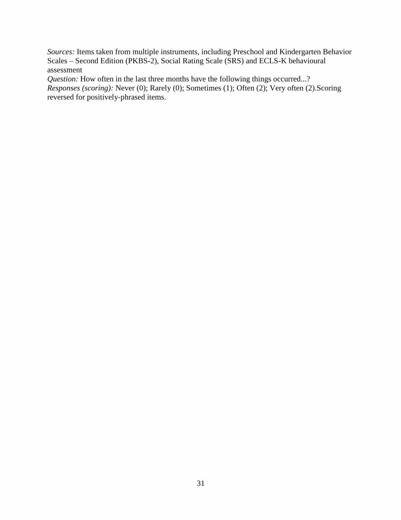
Sources: Items taken from multiple instruments, including Preschool and Kindergarten Behavior
Scales – Second Edition (PKBS-2), Social Rating Scale (SRS) and ECLS-K behavioural
assessment
Question: How often in the last three months have the following things occurred...?
Responses (scoring): Never (0); Rarely (0); Sometimes (1); Often (2); Very often (2).Scoring
reversed for positively-phrased items.

32
Table 5. Average characteristics of families with 4 to 5 year old children, by country
AU
(N = 4,386)
CN
(N = 6812)
UK
(N = 15,460)
US
(N = 8,500)*
Low education (ISCED 2) 8.2% 6.2% 12.2% 10.4%
Middle education (ISCED 3/5B) 53.5% 39.6% 52.9% 56.6%
High education (ISCED 5A/6) 38.4% 54.2% 34.1% 33.0%
Mean household income (SD) 25,569
(15,375)
29,539
(17,983)
27,195
(19,447)
28,534
(27,604)
Single parent household at W3 15.0% 14.4% 19.7% 21.8%
Mother <20 at birth 4.0% 3.4% 7.6% 11.0%
Mother >30 at birth 50.0% 42.6% 40.8% 31.7%
Under 18s in household at W3 2.51
(1.05)
2.25
(0.98)
2.40
(1.05)
2.44
(1.14)
Foreign-born parent 33.0% 31.5% 13.0% 23.4%
White (non-Hispanic for US) - 81.0% 86.7% 54.0%
Black (non-Hispanic for US) - 3.3% 2.8% 13.8%
Hispanic - - - 25.1%
Asian - - - 2.6%
South Asian - 4.9% - -
Pakistani/Bangladeshi - - 4.2% -
Indian - - 1.8% -
Chinese - 2.4% - -
Indigenous (AU)/ Aboriginals (CN) 4.9% 1.9% - -
Mixed - - 3.3% -
Race/ethnicity NOC - 6.6% 1.2% 4.5%
* ECLS-B frequencies rounded to the nearest 50 in accordance with NCES reporting rules.
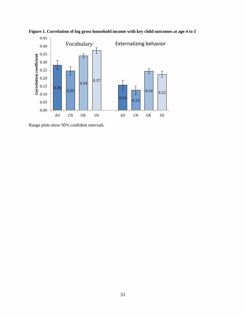
33
Figure 1. Correlation of log gross household income with key child outcomes at age 4 to 5
Range plots show 95% confident intervals.
0.28 0.25
0.34 0.37
0.16 0.13
0.24 0.22
0.00
0.05
0.10
0.15
0.20
0.25
0.30
0.35
0.40
0.45
AU CN UK US AU CN UK US
Co
rre
lati
on
co
eff
icie
nt
Vocabulary Externalizing behavior
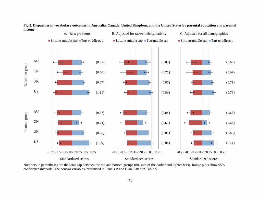
34
Fig 2. Disparities in vocabulary outcomes in Australia, Canada, United Kingdom, and the United States by parental education and parental
income
A. Raw gradients B. Adjusted for race/ethnicity/nativity C. Adjusted for all demographics
Educa
tion g
roup
AU
CN
UK
US
I
nco
me
gro
up
AU
CN
UK
US
Standardized scores Standardized scores Standardized scores
Numbers in parentheses are the total gap between the top and bottom groups (the sum of the darker and lighter bars). Range plots show 95%
confidence intervals. The control variables introduced in Panels B and C are listed in Table 5.
-0.75 -0.5 -0.25 -1E-15 0.25 0.5 0.75
(0.85)
(0.66)
(0.97)
(1.21)
(0.87)
(0.74)
(0.95)
(1.09)
Bottom-middle gap Top-middle gap
-0.75 -0.5 -0.25 -1E-15 0.25 0.5 0.75
(0.83)
(0.71)
(0.87)
(0.86)
(0.84)
(0.63)
(0.81)
(0.84)
Bottom-middle gap Top-middle gap
-0.75 -0.5 -0.25 -1E-15 0.25 0.5 0.75
(0.68)
(0.64)
(0.71)
(0.76)
(0.68)
(0.64)
(0.65)
(0.71)
Bottom-middle gap Top-middle gap
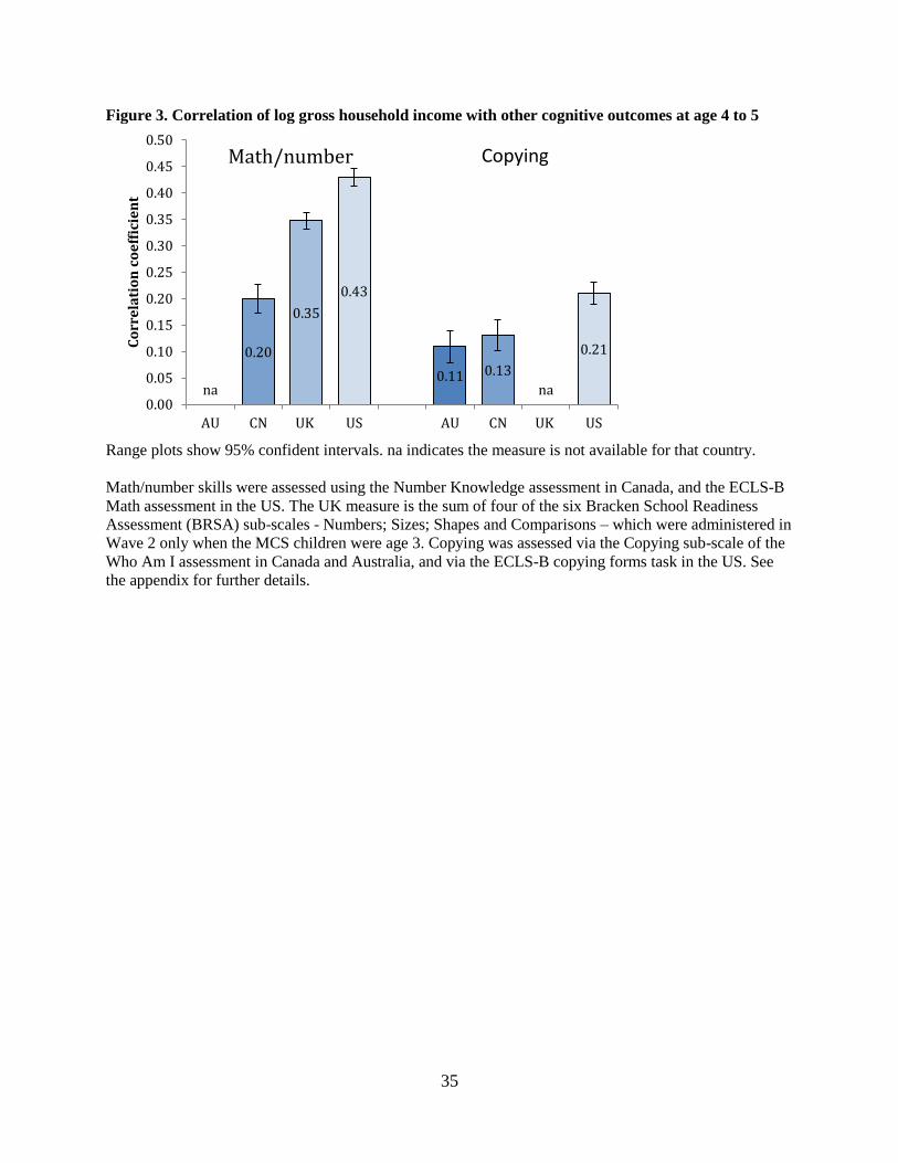
35
Figure 3. Correlation of log gross household income with other cognitive outcomes at age 4 to 5
Range plots show 95% confident intervals. na indicates the measure is not available for that country.
Math/number skills were assessed using the Number Knowledge assessment in Canada, and the ECLS-B
Math assessment in the US. The UK measure is the sum of four of the six Bracken School Readiness
Assessment (BRSA) sub-scales - Numbers; Sizes; Shapes and Comparisons – which were administered in
Wave 2 only when the MCS children were age 3. Copying was assessed via the Copying sub-scale of the
Who Am I assessment in Canada and Australia, and via the ECLS-B copying forms task in the US. See
the appendix for further details.
na
0.20
0.35
0.43
0.11 0.13
na
0.21
0.00
0.05
0.10
0.15
0.20
0.25
0.30
0.35
0.40
0.45
0.50
AU CN UK US AU CN UK US
Co
rre
lati
on
co
eff
icie
nt
Math/number Copying
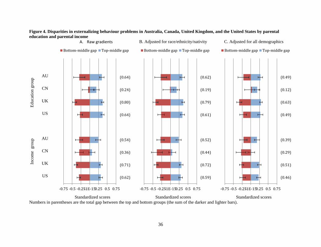
36
Figure 4. Disparities in externalizing behaviour problems in Australia, Canada, United Kingdom, and the United States by parental
education and parental income
A. Raw gradients B. Adjusted for race/ethnicity/nativity C. Adjusted for all demographics
Educa
tion g
roup
AU
CN
UK
US
I
nco
me
gro
up
AU
CN
UK
US
Standardized scores Standardized scores Standardized scores
Numbers in parentheses are the total gap between the top and bottom groups (the sum of the darker and lighter bars).
-0.75 -0.5 -0.25 -1E-15 0.25 0.5 0.75
(0.64)
(0.24)
(0.80)
(0.64)
(0.54)
(0.36)
(0.71)
(0.62)
Bottom-middle gap Top-middle gap
-0.75 -0.5 -0.25 -1E-15 0.25 0.5 0.75
(0.62)
(0.19)
(0.79)
(0.61)
(0.52)
(0.44)
(0.72)
(0.59)
Bottom-middle gap Top-middle gap
-0.75 -0.5 -0.25 -1E-15 0.25 0.5 0.75
(0.49)
(0.12)
(0.63)
(0.49)
(0.39)
(0.29)
(0.51)
(0.46)
Bottom-middle gap Top-middle gap
37
APPENDIX
1. Survey details
Longitudinal Study of Australian Children (LSAC). LSAC contains data from two separate nationally
representative samples of children and their families. The ‗K‘ cohort (not used in our study) comprises
4,983 children born between March 1999 and February 2000, and aged 4-5 during the first round of
interviews. The data used in this study are from the more recent ‗B‘ cohort – 5,107 children born between
March 2003 and February 2004, and aged 0-1 during the first round of interviews.
Random stratified samples were drawn from the Health Insurance Commission database on which
practically all children (and their date of birth) are registered; since it is through this that they have access
to free public health care. The reweighted sample is designed to be representative of all Australian
children in the ‗B‘ cohort age range.
Full waves of face to face interviews have been collected every two years for the LSAC ‗B‘
cohort – when the children were age 0 to 1, 2 to 3 and 4 to 5. In addition, postal questionnaires were sent
to parents at Waves 1.5 and Waves 2.5 (ie., half way through the two year intervals between the main
interviews).
National Longitudinal Study of Children and Youth (NLSCY). Unlike the other datasets used in this study,
the NLSCY is a long-running longitudinal study of Canadian children, with different cohorts brought into
the sample depending on the year. The so-called ―original cohort‖ of 0 to 11 year olds were first surveyed
in 1994/95 (Cycle 1), with information collected every two years since that time. The latest collection of
data occurred in 2006/7 when the original cohort was 12 to 23 years of age (Cycle 7). In addition, each
biennial survey adds an ―Early Childhood Development‖ (ECD) cohort, a representative cohort of 0 to 1
year olds born in 1996, 1998, 2000, 2002, 2004, and 2006. In cycle 7 there are a total of 20,470 children
in all available ECD cohorts.
38
Our analysis draws on two cohorts of children: children born in 2000, age 0-1 in Cycle 4, age 2-3
in Cycle 5, and age 4-5 in Cycle 6; and children born in 2002, age 0-1 in Cycle 5, age 2-3 in Cycle 6, and
age 4-5 in Cycle 7.
The NLSCY sample is meant to be representative of children and is based upon a sampling frame
of all Canadian Households. Typically children are selected from households sampled by Statistics
Canada‘s Labour Force Survey (LFS) that collects labour market data from a national sample of 54000
households on a monthly basis. The LFS is the Canadian equivalent of the US Current Population Survey
(CPS). This is based upon a stratified, multistage design using probability sampling at all stages.
The NLSCY produces three sets of weights at each cycle: two longitudinal, one cross-sectional.
The NLSCY weighting strategy is based on a series of adjustments applied to the NLSCY design weight.
Each child‘s NLSCY design weight is equal to the inverse of his/her probability of selection. The Labour
Force Survey (LFS) subweight accounts for all of the sample design information for the LFS sample. For
the NLSCY, children are selected from the households selected from the LFS. To reflect these additional
sample design steps, the LFS subweight is multiplied by several other factors. The final weight is
obtained by applying nonresponse and post-stratification adjustments to the NLSCY design weight. The
‗post-stratification‘ weight adjustment procedure was carried out to ensure consistency between the
estimates produced by NLSCY and Statistics Canada‘s population estimates by age, sex and province.
The NLSCY collects has three broad components: Child Component, Youth Component and an
Adult Component. The Person Most Knowledgeable (PMK) about the child and his/her spouse answered
the questions in the Adult and Child Component (for children aged 0-17). The Youth component was
used for selected respondents aged 16 and above. The survey has been designed to interview up to two
respondents in the Youth or Child category. The NLSCY therefore makes an important distinction
between ‗households‘ and ‗children/youth‘. The interviews were carried out using computer-assisted
interviewing (CAI) methods and the use of paper questionnaires. The former consisted of computer-
assisted personal interviewing (CAPI) with the help of a laptop as well as computer-assisted telephone
interviewing (CATI).
39
Interviews were conducted in English or French. The interviewers were given freedom to switch
between both languages if the respondent encountered any difficulty in understanding a question or a
phrase. Also, a small number of interviews were conducted in languages other than French or English
with the interviewer translating the questions into the respondent‘s preferred language.
The NLSCY is jointly conducted by Statistics Canada and sponsored by Human Resources and
Social Development Canada (HRSDC). The data is available in Research Data Centres that were
established through a joint effort by Statistics Canada and university consortia. The access to these Data
Centres is restricted to researchers working on projects approved by Social Sciences and Humanities
Research Council (SSHRC) and Statistics Canada.
Millennium Cohort Study (MCS). Children eligible for inclusion in the MCS were those born between 1
September 2000 and 31 August 2001 (for England and Wales), and between 23 November 2000 and 11
January 2002 (for Scotland and Northern Ireland), alive and living in the UK at age nine months.
The geography of electoral wards was used as a sampling frame. There were 11,090 electoral
wards in the UK at the time of sampling, which were combined into 9,548 ‗superwards‘ in order to
eliminate very small units with less than 24 expected births in a year. 398 of these wards and
‗superwards‘ were selected for sampling. The sample is clustered geographically and disproportionately
stratified to over-represent: (1) the three smaller countries of the UK (Wales, Scotland and Northern
Ireland); (2) areas in England with higher minority ethnic populations in 1991 (where at least 30 per cent
of the population were Black or Asian); and (3) disadvantaged areas (drawn from the poorest 25 per cent
of wards based on the Child Poverty Index). Of the 398 wards sampled, 50% were in England, 18% in
Wales, 16% in Scotland and 16% in Northern Ireland; 5% were high ethnic minority wards and 48% were
disadvantaged wards.
A list of all nine month old children living in the sampled wards was derived from Child Benefit
records provided by the Department of Social Security (subsequently Department for Work and Pensions
and then HM Revenue and Customs). Child Benefit claims cover virtually all of the child population
40
except those ineligible due to recent or temporary immigrant status. 27,201 families were identified as
eligible from the Child Benefit records, of which 24,180 (90%) were issued to the field.
Two types of weights are provided with the MCS. The sample design or probability weights are
used to correct for MCS cases having unequal probabilities of selection that result from the stratified
cluster sample design. These are fixed, and do not change over time and vary only by the nine stratum
(advantaged and disadvantaged wards in each of the four countries, plus ethnic wards in England only).
Non-response weights adjust for possible biases generated by systematic unit non-response and vary by
sweep and cohort family. The non-response weight at the current sweep is the inverse of the predicted
probability of responding based on a logistic regression model using data from previous sweep(s).
The MCS surveyed cohort families three times, when the cohort members were roughly 9
months, 3 years and 5 years of age. Future sweeps are planned but not used in this study. At each sweep
there were separate questionnaires for the Main Carer and the Main Carer‘s partner (if present in the
household). Interviews were carried out using computer-assisted personal interview (CAPI) software on a
laptop, and using a confidential computer-assisted self-completion interview (CASI) for sensitive
subjects. Direct child assessments of cognitive ability and anthropomorphic measurements were carried
out at sweeps 2 and 3. Older siblings aged 10 to 15 (in English families only) completed a paper
questionnaire at Sweeps 2 and 3.
Roughly 4% of interviews with the main carer were conducted wholly or partly in a language
other than English in Wave 1, falling to around 2% in Wave 3. Common languages used were: Welsh,
Arabic, Bengali, Gujarati, Hindi, Kurdish, Punjabi, Somali, Tamil, Turkish and Urdu. The child cognitive
assessments were conducted in English only (25 Welsh children completed a Welsh version of the
Naming Vocabulary test, the only assessment for which this option was offered).
The Millennium Cohort Study is funded by the Economic and Social Research Council and a
consortium of Government Departments headed by the Office for National Statistics (ONS). Data are
publicly available from the UK Data Archive.
41
The Early Childhood Longitudinal Study – Birth Cohort (ECLS-B). The ECLS-B selected a nationally
representative probability sample of children born in the United States in 2001. Births were sampled
within a set of primary sampling units (PSUs) and in some cases secondary sampling units (SSUs) in
order to control data collection costs. (A PSU is an individual county or group of contiguous counties. An
SSU is a subdivision of a PSU.) The core ECLS-B sample consists of births sampled within 96 PSUs. An
additional sample of 18 PSUs was selected from a supplemental frame consisting of areas where the
population has a higher proportion of American Indian births (see below). The ECLS-B samples included
births occurring in counties within 46 states and in Washington, D.C.
The ECLS-B was designed to support statistical analyses in the following analytic domains: (1)
child‘s race/ethnicity, as derived from birth certificate data (American Indian including Alaska Natives;
Chinese; Other Asian or Pacific Islander, i.e. excluding Chinese; Hispanic; Black, non-Hispanic; White,
non-Hispanic); (2) birth weight (very low, moderately low and normal) and (3) plurality (twin and non-
twin). When combined, these analytic domains result in 36 distinct birth certificate sampling strata. Six
strata required oversampling: the American Indian, Chinese, and Other Asian/Pacific Islander groups;
those with very low birth weight (under 1,500 grams) and those with moderately low birth weight
(between 1,500 and 2,500 grams); and twins.
Children were sampled via registered births from the National Center for Health Statistics
(NCHS) vital statistics system. Individual birth certificates within PSUs or SSUs were sampled from data
files provided by state registrars. Within each case stratum, each sampled birth had an equal overall
probability of selection. Membership of an ECLS-B PSU was determined using state and county of
occurrence, although birth certificates also provide information on state of residence. Approximately
14,000 births were sampled and fielded and yielded 10,688 9-month completed cases.
The ECLS-B weights were developed in three steps: (1) base weights were calculated using the
overall selection probabilities; (2) weights were adjusted for survey nonresponse; and (3) raking
(adjusting sums of weights to known or estimated totals) was used to adjust for undercoverage and to
improve precision of survey estimates. The development of the ECLS-B weights was a sequential
42
process. The 9-month weights were developed from the base weight. Weights for subsequent sweeps were
then developed as adjustments to the weights from the previous wave.
The ECLS-B surveyed cohort families three times, when the cohort members were roughly 9
months and 2 years of age, and during the preschool year when most cohort members were 4 years of age.
A future kindergarten wave is planned but not used in this study. A Parent Computer-Assisted Personal
Interview (CAPI) was administered at each of the three sweeps, consisting of an in-person interview in
which the interviewer asked questions aloud and entered the responses in a computer. In addition, for
items that could be considered sensitive, parent self-completion intstruments were used.
The full scope of the ECLS-B includes a number of data collection instruments not used in this
study. These are Resident and Non-resident Father Questionnaires; selected variables taken directly from
the birth certificate; a Child Care Provider telephone interview; and in some cases a Child Care
Observation.
Computer-assisted personal interviews (CAPIs) and self-administered paper questionnaires were
available in English and Spanish versions, and bilingual interviewers were trained to conduct interviews
in either English or Spanish. An interpreter, either a community or household member, was used for
families who spoke languages other than English or Spanish. Around 6-7% of parent interviews were
conducted in Spanish at each sweep, and further 1.5-2% were conducted in a language other than English
and Spanish. A Spanish version of the ECLS-B Preschool Direct Cognitive Assessment (Wave 3) was
used in the field when necessary, but assessment scores were not computed/provided because sample
sizes were too small (n=120). Hence all of the preschool wave assessment data that is usable was
administered in English.
The primary sponsor of the ECLS-B is the National Center for Education Statistics (NCES),
Institute of Education Sciences (IES), U.S. Department of Education (ED). Due to NCES' confidentiality
legislation, ECLS-B data in micro-data form (i.e., CD-ROM) are available only through a restricted-use
data license agreement.
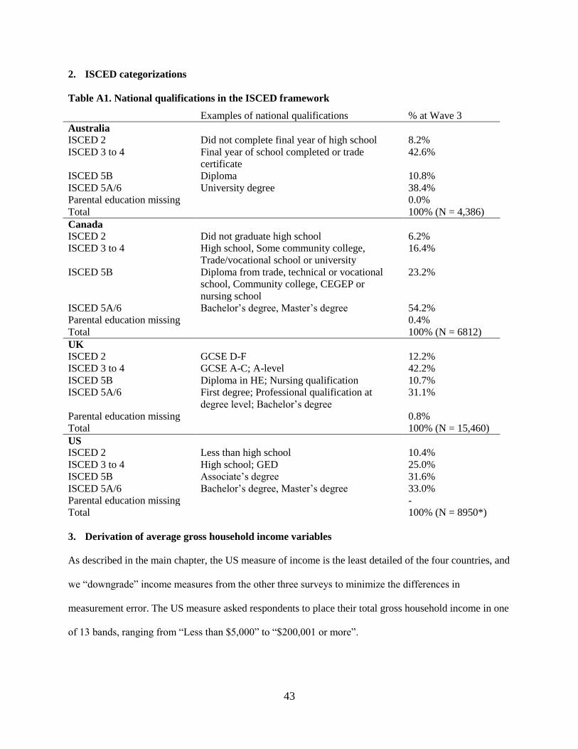
43
2. ISCED categorizations
Table A1. National qualifications in the ISCED framework
Examples of national qualifications % at Wave 3
Australia
ISCED 2 Did not complete final year of high school 8.2%
ISCED 3 to 4 Final year of school completed or trade
certificate
42.6%
ISCED 5B Diploma 10.8%
ISCED 5A/6 University degree 38.4%
Parental education missing 0.0%
Total 100% (N = 4,386)
Canada
ISCED 2 Did not graduate high school 6.2%
ISCED 3 to 4 High school, Some community college,
Trade/vocational school or university
16.4%
ISCED 5B Diploma from trade, technical or vocational
school, Community college, CEGEP or
nursing school
23.2%
ISCED 5A/6 Bachelor‘s degree, Master‘s degree 54.2%
Parental education missing 0.4%
Total 100% (N = 6812)
UK
ISCED 2 GCSE D-F 12.2%
ISCED 3 to 4 GCSE A-C; A-level 42.2%
ISCED 5B Diploma in HE; Nursing qualification 10.7%
ISCED 5A/6 First degree; Professional qualification at
degree level; Bachelor‘s degree
31.1%
Parental education missing 0.8%
Total 100% (N = 15,460)
US
ISCED 2 Less than high school 10.4%
ISCED 3 to 4 High school; GED 25.0%
ISCED 5B Associate‘s degree 31.6%
ISCED 5A/6 Bachelor‘s degree, Master‘s degree 33.0%
Parental education missing -
Total 100% (N = 8950*)
3. Derivation of average gross household income variables
As described in the main chapter, the US measure of income is the least detailed of the four countries, and
we ―downgrade‖ income measures from the other three surveys to minimize the differences in
measurement error. The US measure asked respondents to place their total gross household income in one
of 13 bands, ranging from ―Less than $5,000‖ to ―$200,001 or more‖.
44
First, we calculated the proportion of families falling into each of the 13 bands at each of three
waves, separately for two-parent and single-parent households. To illustrate 1.7% of two-parent
households reported incomes in the lowest band at Wave 1 and 3.0% reported incomes in the second
lowest band. Equivalent percentages of the sample of single-parent households were 17.8% and 15.6%.
The basis of our income harmonization was then to define categorical income variables -- for each
country, wave and family structure group – with the same distributions as the US variables. The
categorical variables were then converted back to a ―lumpy‖ continuous variables by assigning a
representative dollar value to each band. This procedure differed slightly across surveys.
Australia and Canada. The income questions in both the LSAC and the NLSCY asked for gross
household income in a continuous format. After dividing families into the proportions described above on
the basis of their reported income, each family in a given band was assigned the median value of income
in that band, overwriting the family-specific reported value.
UK. Income questions in the MCS related to net rather than gross household income, and also
required responses in bands, although in this case 19 bands were offered with the boundaries differing for
single- and two-parent families. To deal with this, we used external nationally representative data from
the Family Resources Survey (FRS) 2001 to 2007 on the gross and net incomes of families with children
under 6. The median value of gross income for FRS families with net incomes within each pair boundary
values was calculated and assigned to the relevant MCS families. Hence this step both converted net to
gross values and created continuous variables from the MCS banded data in the most detailed way
possible. This intermediary variable was then transformed in the same way as the Australian and
Canadian continuous gross income variables, by dividing it up according to the US distribution and over-
writing with the median band value.
US. In order to assign a dollar value to each of the US income bands, and in particular to ―close‖
to open top band, we again use external nationally representative data, in this case from the June Current
Population Survey (CPS). The value of income assigned to each band is the median gross income of
families with children under 6 with income inside the boundary values.
45
For all countries these nominal derived gross household income variables were deflated to 2006
values using national price indices, converted to US dollars using OECD purchasing power parity (PPP)
indices, and normalized by the square root of household size. The three observations of real gross
equivalized household income for each family were then averaged and the survey weights were used to
define nationally-representative quintile boundaries.
More specifically, the Australian price indices for the three waves of the data were 2004 = 0.941,
2006 = 1, and 2008 = 1.068 (Source: ABS 6401.0, Annual CPI), the Canadian indices were 2000 = 0.874,
2002 = 0.917, 2004 = 0.958 and 2006 = 1 (Source: Statistics Canada, CPI for Canada V41690973 series),
the UK 2001 = 0.875, 2002 = 0.889, 2003 = 0.915, 2004 = 0.942, 2005 = 0.969, 2006 = 1, 2007 = 1.043
(Source: ONS, All Items RPI) and the US 2001 = 0.878, 2002 = 0.892, 2003 = 0.913, 2004 = 0.937, 2005
= 0.969, 2006 = 1, 2007 = 1.028 (Source: BLS CPI-U). The PPP indices used were AU = 1.375, CN =
1.210, UK = 0.617 and US = 1 (Source: PPP index for 'actual individual consumption' for 2006,
SourceOECD National Accounts Statistics, Volume I - Exchange Rate, PPPs, and Population Vol 2009
release 01, downloaded 15 Dec 09).
4. Additional information on outcome measures
As described in the main text, the picture vocabulary tests used in the Australian, Canadian and US
surveys all used items from the Peabody Picture Vocabulary Test (PPVT). The instruments administered,
however, were not identical. The LSAC used a short version of the Third Edition of the PPVT (PPVT-
III), adapted specifically for the survey and containing 40 items – 20 core, 10 basal (to which children
performing poorly on the core items were routed), and 10 ceiling items (for children socring highly on the
core items). The NLSCY administed the PPVT Revised Version in full (PPVT-R; the prior version to the
PPVT-III), with a French adaptation (EVIP) available for all French-speakers. The ECLS-B, like the
LSAC, used only selected items from the PPVT-III, but in this case only 15 items were selected in total.
Early math and number skills were assessed in three of the countries, Australia being the
exception. We provide some results relating to these outcomes but note they were assessed in quite
46
different ways in different surveys and results may not be as comparable across countries as for some
other outcomes. The Canadian Number Knowledge assessment is a mental arithmetic test designed to
measure children‘s comprehension of the system of whole numbers. Children were not permitted to use a
pencil and paper but instead were required to rely on a ―mental counting line‖ in order to answer the
orally-given questions. The ECLS-B Mathematics assessment was designed specifically for the US
survey and included questions in following content areas: number sense, geometry, counting, operations,
and patterns. As with the vocabulary assessments, the items administered were routed according to the
child‘s responses and scored consistently using IRT techniques. The UK dataset contains no assessments
of math skills in Wave 3. However, in Wave 2 (when the children were 3 years of age) the Bracken
School Readiness Assessment (BRSA) was administered, which is composed of six sub-scales. We derive
a measure of math skills as the sum of the Numbers, Sizes, Comparisons and Shapes sub-scales, a broad
definition that is perhaps most comparable with the US Mathematics assessment. Assessments of copying
skills are available for children in all countries except the UK. The tasks are designed to assess the child‘s
ability to conceptualize and reconstruct a geometrical shape and provide a non-verbal test of cognitive
ability that provides a contrast to the verbal vocabulary measure. The use of the ability to copy
geometrical figures to assess the level of development in children has been long established, indeed dating
back to the original Simon Binet test. Research indicates that copying skills are strongly associated with
subsequent school achievement, are valid across different cultural groups, and provide a reliable measure
of development at the time of assessment (de Lemos, 2002). In all three countries the child recorded his or
her response in a booklet, which was then scored centrally by trained researchers. The Australian and
Canadian children were assessed using the same instrument: the Copying scale of the Who Am I (WAI)
assessment, which requires children to copy five shapes (circle, triangle, cross, square, and diamond) with
each response assessed on a four-point scale. In the US task the child was asked to copy seven shapes
(vertical line, horizontal line, circle, square, cross, triangle, and asterisk) with each items scored either one
(a pass) or zero (fail).
47
Several other cognitive assessment measures are available for single countries or pairs of
countries only. For Canada and Australia, the Symbols sub-scale of the WAI assessment, composed of a
set of five writing tasks (printing their name, printing some letters, numbers, words and a sentence),
assesses the ability of the child to understand and use symbolic representations such as numbers, letters
and words. The WAI Total score is the sum of the WAI Copying and Symbols sub-scales. The US
Literacy Assessment, again designed specifically for the ECLS-B and using IRT scoring techniques,
assesses a range of content areas related to emergent literacy: letter recognition, in both receptive and
expressive modes; letter sounds; early reading (recognition of simple words); phonological awareness;
knowledge of print conventions; and matching words. Finally, the total BRSA score for the UK children
(the sum of the four math sub-scales plus the Letters and Colors sub-scales) provides a summary measure
of cognitive ability that combines a number of literacy and math skills.
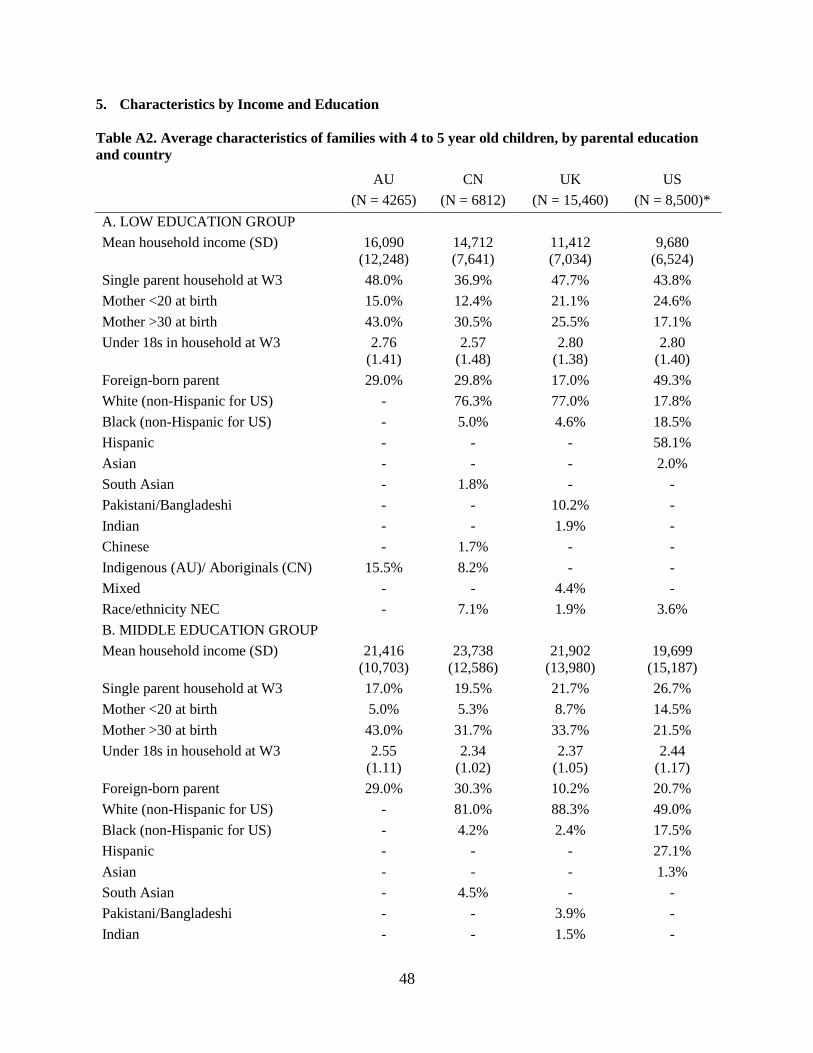
48
5. Characteristics by Income and Education
Table A2. Average characteristics of families with 4 to 5 year old children, by parental education
and country
AU
(N = 4265)
CN
(N = 6812)
UK
(N = 15,460)
US
(N = 8,500)*
A. LOW EDUCATION GROUP
Mean household income (SD) 16,090
(12,248)
14,712
(7,641)
11,412
(7,034)
9,680
(6,524)
Single parent household at W3 48.0% 36.9% 47.7% 43.8%
Mother <20 at birth 15.0% 12.4% 21.1% 24.6%
Mother >30 at birth 43.0% 30.5% 25.5% 17.1%
Under 18s in household at W3 2.76
(1.41)
2.57
(1.48)
2.80
(1.38)
2.80
(1.40)
Foreign-born parent 29.0% 29.8% 17.0% 49.3%
White (non-Hispanic for US) - 76.3% 77.0% 17.8%
Black (non-Hispanic for US) - 5.0% 4.6% 18.5%
Hispanic - - - 58.1%
Asian - - - 2.0%
South Asian - 1.8% - -
Pakistani/Bangladeshi - - 10.2% -
Indian - - 1.9% -
Chinese - 1.7% - -
Indigenous (AU)/ Aboriginals (CN) 15.5% 8.2% - -
Mixed - - 4.4% -
Race/ethnicity NEC - 7.1% 1.9% 3.6%
B. MIDDLE EDUCATION GROUP
Mean household income (SD) 21,416
(10,703)
23,738
(12,586)
21,902
(13,980)
19,699
(15,187)
Single parent household at W3 17.0% 19.5% 21.7% 26.7%
Mother <20 at birth 5.0% 5.3% 8.7% 14.5%
Mother >30 at birth 43.0% 31.7% 33.7% 21.5%
Under 18s in household at W3 2.55
(1.11)
2.34
(1.02)
2.37
(1.05)
2.44
(1.17)
Foreign-born parent 29.0% 30.3% 10.2% 20.7%
White (non-Hispanic for US) - 81.0% 88.3% 49.0%
Black (non-Hispanic for US) - 4.2% 2.4% 17.5%
Hispanic - - - 27.1%
Asian - - - 1.3%
South Asian - 4.5% - -
Pakistani/Bangladeshi - - 3.9% -
Indian - - 1.5% -
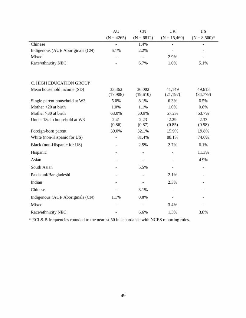
49
AU
(N = 4265)
CN
(N = 6812)
UK
(N = 15,460)
US
(N = 8,500)*
Chinese - 1.4% - -
Indigenous (AU)/ Aboriginals (CN) 6.1% 2.2% - -
Mixed - - 2.9% -
Race/ethnicity NEC - 6.7% 1.0% 5.1%
C. HIGH EDUCATION GROUP
Mean household income (SD) 33,362
(17,908)
36,002
(19,610)
41,149
(21,197)
49,613
(34,779)
Single parent household at W3 5.0% 8.1% 6.3% 6.5%
Mother <20 at birth 1.0% 1.1% 1.0% 0.8%
Mother >30 at birth 63.0% 50.9% 57.2% 53.7%
Under 18s in household at W3 2.41
(0.86)
2.23
(0.87)
2.29
(0.85)
2.33
(0.98)
Foreign-born parent 39.0% 32.1% 15.9% 19.8%
White (non-Hispanic for US) - 81.4% 88.1% 74.0%
Black (non-Hispanic for US) - 2.5% 2.7% 6.1%
Hispanic - - - 11.3%
Asian - - - 4.9%
South Asian - 5.5% - -
Pakistani/Bangladeshi - - 2.1% -
Indian - - 2.3% -
Chinese - 3.1% - -
Indigenous (AU)/ Aboriginals (CN) 1.1% 0.8% - -
Mixed - - 3.4% -
Race/ethnicity NEC - 6.6% 1.3% 3.8%
* ECLS-B frequencies rounded to the nearest 50 in accordance with NCES reporting rules.
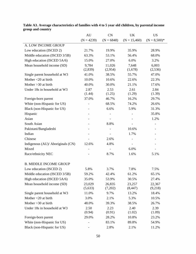
50
Table A3. Average characteristics of families with 4 to 5 year old children, by parental income
group and country
AU
(N = 4239)
CN
(N = 6848)
UK
(N = 15,460)
US
(N = 8,500)*
A. LOW INCOME GROUP
Low education (ISCED 2) 21.7% 19.9% 35.9% 28.9%
Middle education (ISCED 3/5B) 63.3% 53.1% 56.4% 68.0%
High education (ISCED 5A/6) 15.0% 27.0% 6.0% 3.2%
Mean household income (SD) 9,784
(2,839)
11,026
(2,954)
7,648
(1,678)
6,003
(2,536)
Single parent household at W3 41.0% 38.5% 55.7% 47.0%
Mother <20 at birth 10.0% 10.6% 22.6% 22.3%
Mother >30 at birth 40.0% 30.0% 21.1% 17.6%
Under 18s in household at W3 2.87
(1.44)
2.53
(1.25)
2.61
(1.29)
2.84
(1.39)
Foreign-born parent 37.0% 46.7% 16.2% 29.7%
White (non-Hispanic for US) - 68.5% 74.2% 26.6%
Black (non-Hispanic for US) - 6.6% 5.9% 31.3%
Hispanic - - - 35.8%
Asian - - - 1.2%
South Asian - 8.8% - -
Pakistani/Bangladeshi - - 10.6% -
Indian - - 1.7% -
Chinese - 2.6% - -
Indigenous (AU)/ Aboriginals (CN) 12.6% 4.8% - -
Mixed - - 6.0% -
Race/ethnicity NEC - 8.7% 1.6% 5.1%
B. MIDDLE INCOME GROUP
Low education (ISCED 2) 5.8% 3.7% 7.8% 7.5%
Middle education (ISCED 3/5B) 59.2% 42.4% 61.2% 65.1%
High education (ISCED 5A/6) 35.0% 53.9% 30.5% 27.4%
Mean household income (SD) 23,029
(5,633)
26,835
(7,202)
23,257
(8,447)
22,367
(9,218)
Single parent household at W3 11.0% 9.7% 13.2% 18.4%
Mother <20 at birth 3.0% 2.1% 5.3% 10.5%
Mother >30 at birth 48.0% 39.3% 38.5% 26.7%
Under 18s in household at W3 2.50
(0.94)
2.23
(0.91)
2.40
(1.02)
2.39
(1.09)
Foreign-born parent 29.0% 28.2% 10.8% 23.2%
White (non-Hispanic for US) - 83.1% 89.8% 54.9%
Black (non-Hispanic for US) - 2.8% 2.1% 11.2%
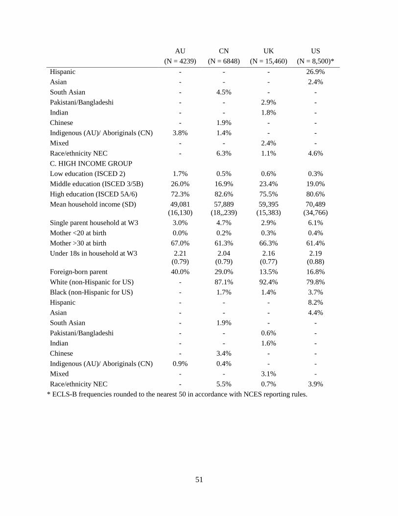
51
AU
(N = 4239)
CN
(N = 6848)
UK
(N = 15,460)
US
(N = 8,500)*
Hispanic - - - 26.9%
Asian - - - 2.4%
South Asian - 4.5% - -
Pakistani/Bangladeshi - - 2.9% -
Indian - - 1.8% -
Chinese - 1.9% - -
Indigenous (AU)/ Aboriginals (CN) 3.8% 1.4% - -
Mixed - - 2.4% -
Race/ethnicity NEC - 6.3% 1.1% 4.6%
C. HIGH INCOME GROUP
Low education (ISCED 2) 1.7% 0.5% 0.6% 0.3%
Middle education (ISCED 3/5B) 26.0% 16.9% 23.4% 19.0%
High education (ISCED 5A/6) 72.3% 82.6% 75.5% 80.6%
Mean household income (SD) 49,081
(16,130)
57,889
(18,,239)
59,395
(15,383)
70,489
(34,766)
Single parent household at W3 3.0% 4.7% 2.9% 6.1%
Mother <20 at birth 0.0% 0.2% 0.3% 0.4%
Mother >30 at birth 67.0% 61.3% 66.3% 61.4%
Under 18s in household at W3 2.21
(0.79)
2.04
(0.79)
2.16
(0.77)
2.19
(0.88)
Foreign-born parent 40.0% 29.0% 13.5% 16.8%
White (non-Hispanic for US) - 87.1% 92.4% 79.8%
Black (non-Hispanic for US) - 1.7% 1.4% 3.7%
Hispanic - - - 8.2%
Asian - - - 4.4%
South Asian - 1.9% - -
Pakistani/Bangladeshi - - 0.6% -
Indian - - 1.6% -
Chinese - 3.4% - -
Indigenous (AU)/ Aboriginals (CN) 0.9% 0.4% - -
Mixed - - 3.1% -
Race/ethnicity NEC - 5.5% 0.7% 3.9%
* ECLS-B frequencies rounded to the nearest 50 in accordance with NCES reporting rules.
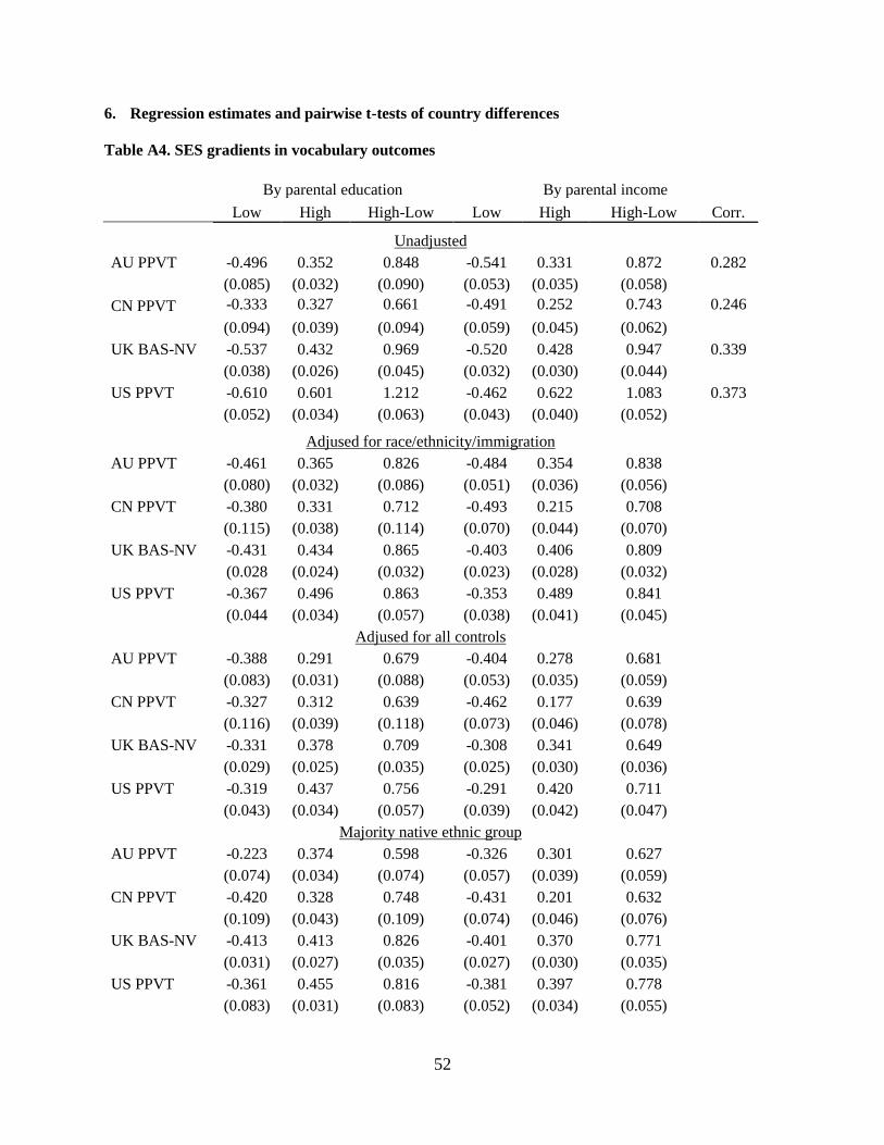
52
6. Regression estimates and pairwise t-tests of country differences
Table A4. SES gradients in vocabulary outcomes
By parental education By parental income
Low High High-Low Low High High-Low Corr.
Unadjusted
AU PPVT -0.496 0.352 0.848 -0.541 0.331 0.872 0.282
(0.085) (0.032) (0.090) (0.053) (0.035) (0.058)
CN PPVT -0.333 0.327 0.661 -0.491 0.252 0.743 0.246
(0.094) (0.039) (0.094) (0.059) (0.045) (0.062)
UK BAS-NV -0.537 0.432 0.969 -0.520 0.428 0.947 0.339
(0.038) (0.026) (0.045) (0.032) (0.030) (0.044)
US PPVT -0.610 0.601 1.212 -0.462 0.622 1.083 0.373
(0.052) (0.034) (0.063) (0.043) (0.040) (0.052)
Adjused for race/ethnicity/immigration
AU PPVT -0.461 0.365 0.826 -0.484 0.354 0.838
(0.080) (0.032) (0.086) (0.051) (0.036) (0.056)
CN PPVT -0.380 0.331 0.712 -0.493 0.215 0.708
(0.115) (0.038) (0.114) (0.070) (0.044) (0.070)
UK BAS-NV -0.431 0.434 0.865 -0.403 0.406 0.809
(0.028 (0.024) (0.032) (0.023) (0.028) (0.032)
US PPVT -0.367 0.496 0.863 -0.353 0.489 0.841
(0.044 (0.034) (0.057) (0.038) (0.041) (0.045)
Adjused for all controls
AU PPVT -0.388 0.291 0.679 -0.404 0.278 0.681
(0.083) (0.031) (0.088) (0.053) (0.035) (0.059)
CN PPVT -0.327 0.312 0.639 -0.462 0.177 0.639
(0.116) (0.039) (0.118) (0.073) (0.046) (0.078)
UK BAS-NV -0.331 0.378 0.709 -0.308 0.341 0.649
(0.029) (0.025) (0.035) (0.025) (0.030) (0.036)
US PPVT -0.319 0.437 0.756 -0.291 0.420 0.711
(0.043) (0.034) (0.057) (0.039) (0.042) (0.047)
Majority native ethnic group
AU PPVT -0.223 0.374 0.598 -0.326 0.301 0.627
(0.074) (0.034) (0.074) (0.057) (0.039) (0.059)
CN PPVT -0.420 0.328 0.748 -0.431 0.201 0.632
(0.109) (0.043) (0.109) (0.074) (0.046) (0.076)
UK BAS-NV -0.413 0.413 0.826 -0.401 0.370 0.771
(0.031) (0.027) (0.035) (0.027) (0.030) (0.035)
US PPVT -0.361 0.455 0.816 -0.381 0.397 0.778
(0.083) (0.031) (0.083) (0.052) (0.034) (0.055)
53
Standard errors (adjusted for complex survey design) in parenthesis. All numbers (other than correlations)
are standard deviation units. Low and High denote the deviations in the mean outcome from the (omitted)
middle SES group among the low and high SES groups respectively.
Race/ethnicity/immigration controls: Dummy variable for either parent foreign-born; set of country-
specific dummies for race/ethnic category (see Table 5).
All controls: Race/ethnicity/immigration controls described above, plus: dummies for mother<20;
mother>30; single parent household at Wave 3; number of under-18s in the household at Wave 3
(continuous variable).
Majority native ethnic group defined as neither parent foreign-born and race/ethnicity as follows (% total
sample): AU – Non-indigenous (67%); CN – White (70%); UK – White (79%); US – White non-Hispanic
(42%).
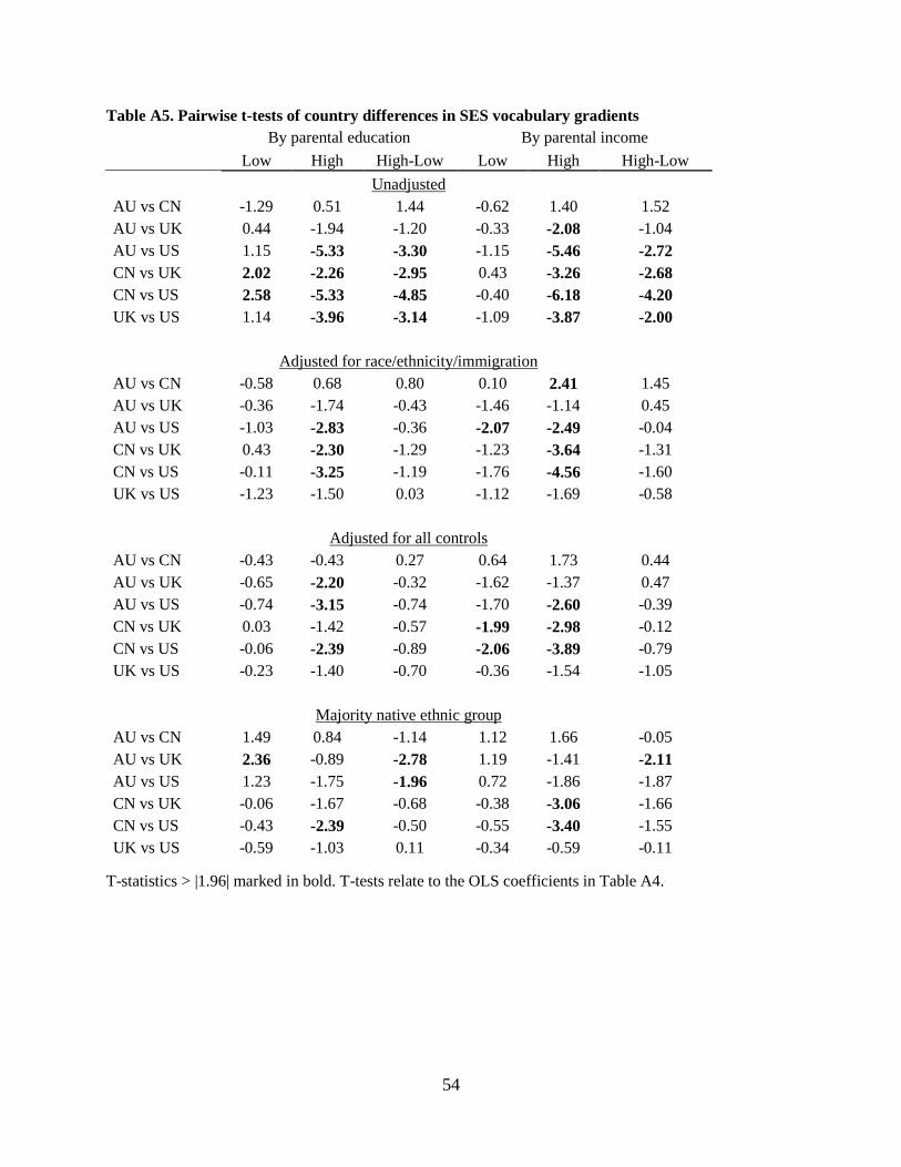
54
Table A5. Pairwise t-tests of country differences in SES vocabulary gradients
By parental education By parental income
Low High High-Low Low High High-Low
Unadjusted
AU vs CN -1.29 0.51 1.44 -0.62 1.40 1.52
AU vs UK 0.44 -1.94 -1.20 -0.33 -2.08 -1.04
AU vs US 1.15 -5.33 -3.30 -1.15 -5.46 -2.72
CN vs UK 2.02 -2.26 -2.95 0.43 -3.26 -2.68
CN vs US 2.58 -5.33 -4.85 -0.40 -6.18 -4.20
UK vs US 1.14 -3.96 -3.14 -1.09 -3.87 -2.00
Adjusted for race/ethnicity/immigration
AU vs CN -0.58 0.68 0.80 0.10 2.41 1.45
AU vs UK -0.36 -1.74 -0.43 -1.46 -1.14 0.45
AU vs US -1.03 -2.83 -0.36 -2.07 -2.49 -0.04
CN vs UK 0.43 -2.30 -1.29 -1.23 -3.64 -1.31
CN vs US -0.11 -3.25 -1.19 -1.76 -4.56 -1.60
UK vs US -1.23 -1.50 0.03 -1.12 -1.69 -0.58
Adjusted for all controls
AU vs CN -0.43 -0.43 0.27 0.64 1.73 0.44
AU vs UK -0.65 -2.20 -0.32 -1.62 -1.37 0.47
AU vs US -0.74 -3.15 -0.74 -1.70 -2.60 -0.39
CN vs UK 0.03 -1.42 -0.57 -1.99 -2.98 -0.12
CN vs US -0.06 -2.39 -0.89 -2.06 -3.89 -0.79
UK vs US -0.23 -1.40 -0.70 -0.36 -1.54 -1.05
Majority native ethnic group
AU vs CN 1.49 0.84 -1.14 1.12 1.66 -0.05
AU vs UK 2.36 -0.89 -2.78 1.19 -1.41 -2.11
AU vs US 1.23 -1.75 -1.96 0.72 -1.86 -1.87
CN vs UK -0.06 -1.67 -0.68 -0.38 -3.06 -1.66
CN vs US -0.43 -2.39 -0.50 -0.55 -3.40 -1.55
UK vs US -0.59 -1.03 0.11 -0.34 -0.59 -0.11
T-statistics > |1.96| marked in bold. T-tests relate to the OLS coefficients in Table A4.
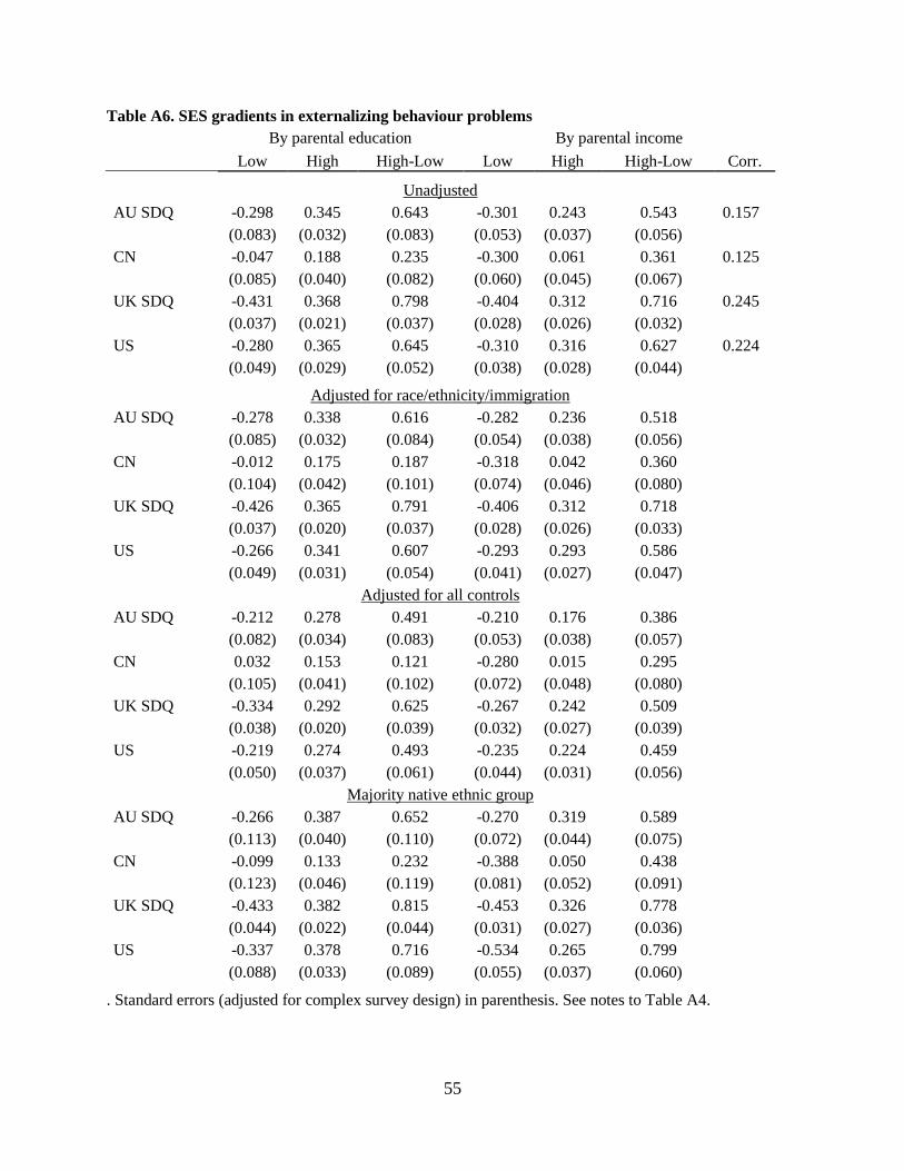
55
Table A6. SES gradients in externalizing behaviour problems
By parental education By parental income
Low High High-Low Low High High-Low Corr.
Unadjusted
AU SDQ -0.298 0.345 0.643 -0.301 0.243 0.543 0.157
(0.083) (0.032) (0.083) (0.053) (0.037) (0.056)
CN -0.047 0.188 0.235 -0.300 0.061 0.361 0.125
(0.085) (0.040) (0.082) (0.060) (0.045) (0.067)
UK SDQ -0.431 0.368 0.798 -0.404 0.312 0.716 0.245
(0.037) (0.021) (0.037) (0.028) (0.026) (0.032)
US -0.280 0.365 0.645 -0.310 0.316 0.627 0.224
(0.049) (0.029) (0.052) (0.038) (0.028) (0.044)
Adjusted for race/ethnicity/immigration
AU SDQ -0.278 0.338 0.616 -0.282 0.236 0.518
(0.085) (0.032) (0.084) (0.054) (0.038) (0.056)
CN -0.012 0.175 0.187 -0.318 0.042 0.360
(0.104) (0.042) (0.101) (0.074) (0.046) (0.080)
UK SDQ -0.426 0.365 0.791 -0.406 0.312 0.718
(0.037) (0.020) (0.037) (0.028) (0.026) (0.033)
US -0.266 0.341 0.607 -0.293 0.293 0.586
(0.049) (0.031) (0.054) (0.041) (0.027) (0.047)
Adjusted for all controls
AU SDQ -0.212 0.278 0.491 -0.210 0.176 0.386
(0.082) (0.034) (0.083) (0.053) (0.038) (0.057)
CN 0.032 0.153 0.121 -0.280 0.015 0.295
(0.105) (0.041) (0.102) (0.072) (0.048) (0.080)
UK SDQ -0.334 0.292 0.625 -0.267 0.242 0.509
(0.038) (0.020) (0.039) (0.032) (0.027) (0.039)
US -0.219 0.274 0.493 -0.235 0.224 0.459
(0.050) (0.037) (0.061) (0.044) (0.031) (0.056)
Majority native ethnic group
AU SDQ -0.266 0.387 0.652 -0.270 0.319 0.589
(0.113) (0.040) (0.110) (0.072) (0.044) (0.075)
CN -0.099 0.133 0.232 -0.388 0.050 0.438
(0.123) (0.046) (0.119) (0.081) (0.052) (0.091)
UK SDQ -0.433 0.382 0.815 -0.453 0.326 0.778
(0.044) (0.022) (0.044) (0.031) (0.027) (0.036)
US -0.337 0.378 0.716 -0.534 0.265 0.799
(0.088) (0.033) (0.089) (0.055) (0.037) (0.060)
. Standard errors (adjusted for complex survey design) in parenthesis. See notes to Table A4.
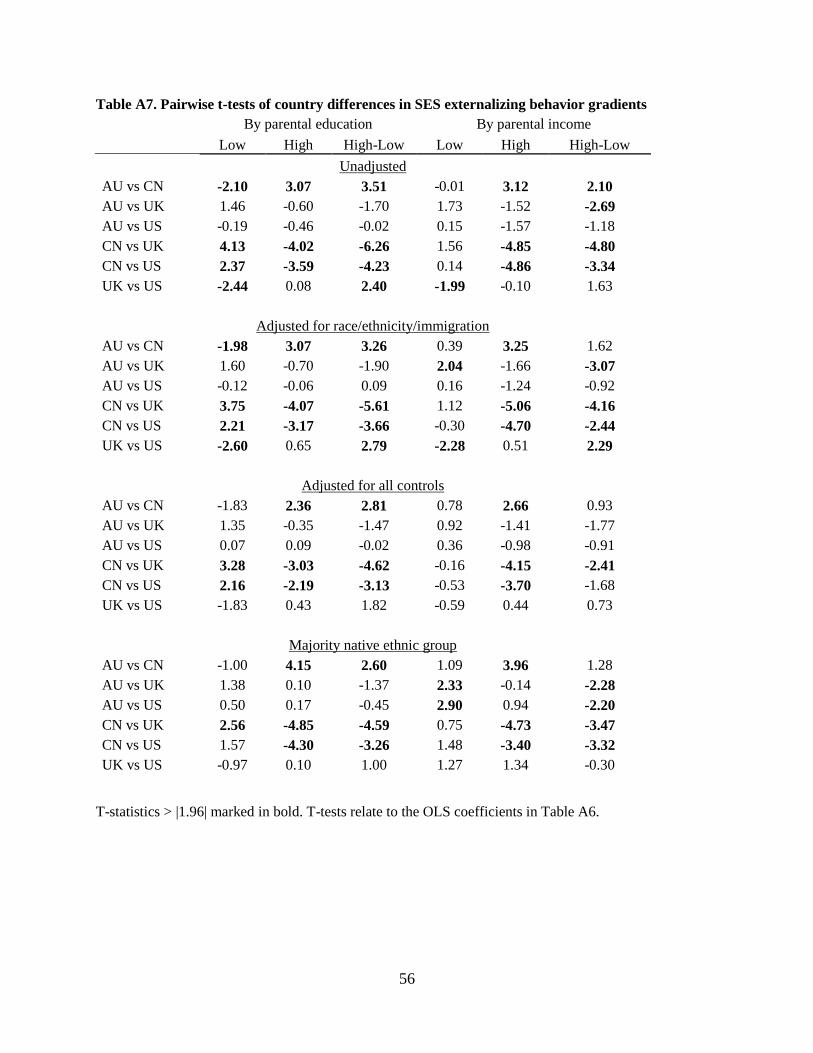
56
Table A7. Pairwise t-tests of country differences in SES externalizing behavior gradients
By parental education By parental income
Low High High-Low Low High High-Low
Unadjusted
AU vs CN -2.10 3.07 3.51 -0.01 3.12 2.10
AU vs UK 1.46 -0.60 -1.70 1.73 -1.52 -2.69
AU vs US -0.19 -0.46 -0.02 0.15 -1.57 -1.18
CN vs UK 4.13 -4.02 -6.26 1.56 -4.85 -4.80
CN vs US 2.37 -3.59 -4.23 0.14 -4.86 -3.34
UK vs US -2.44 0.08 2.40 -1.99 -0.10 1.63
Adjusted for race/ethnicity/immigration
AU vs CN -1.98 3.07 3.26 0.39 3.25 1.62
AU vs UK 1.60 -0.70 -1.90 2.04 -1.66 -3.07
AU vs US -0.12 -0.06 0.09 0.16 -1.24 -0.92
CN vs UK 3.75 -4.07 -5.61 1.12 -5.06 -4.16
CN vs US 2.21 -3.17 -3.66 -0.30 -4.70 -2.44
UK vs US -2.60 0.65 2.79 -2.28 0.51 2.29
Adjusted for all controls
AU vs CN -1.83 2.36 2.81 0.78 2.66 0.93
AU vs UK 1.35 -0.35 -1.47 0.92 -1.41 -1.77
AU vs US 0.07 0.09 -0.02 0.36 -0.98 -0.91
CN vs UK 3.28 -3.03 -4.62 -0.16 -4.15 -2.41
CN vs US 2.16 -2.19 -3.13 -0.53 -3.70 -1.68
UK vs US -1.83 0.43 1.82 -0.59 0.44 0.73
Majority native ethnic group
AU vs CN -1.00 4.15 2.60 1.09 3.96 1.28
AU vs UK 1.38 0.10 -1.37 2.33 -0.14 -2.28
AU vs US 0.50 0.17 -0.45 2.90 0.94 -2.20
CN vs UK 2.56 -4.85 -4.59 0.75 -4.73 -3.47
CN vs US 1.57 -4.30 -3.26 1.48 -3.40 -3.32
UK vs US -0.97 0.10 1.00 1.27 1.34 -0.30
T-statistics > |1.96| marked in bold. T-tests relate to the OLS coefficients in Table A6.
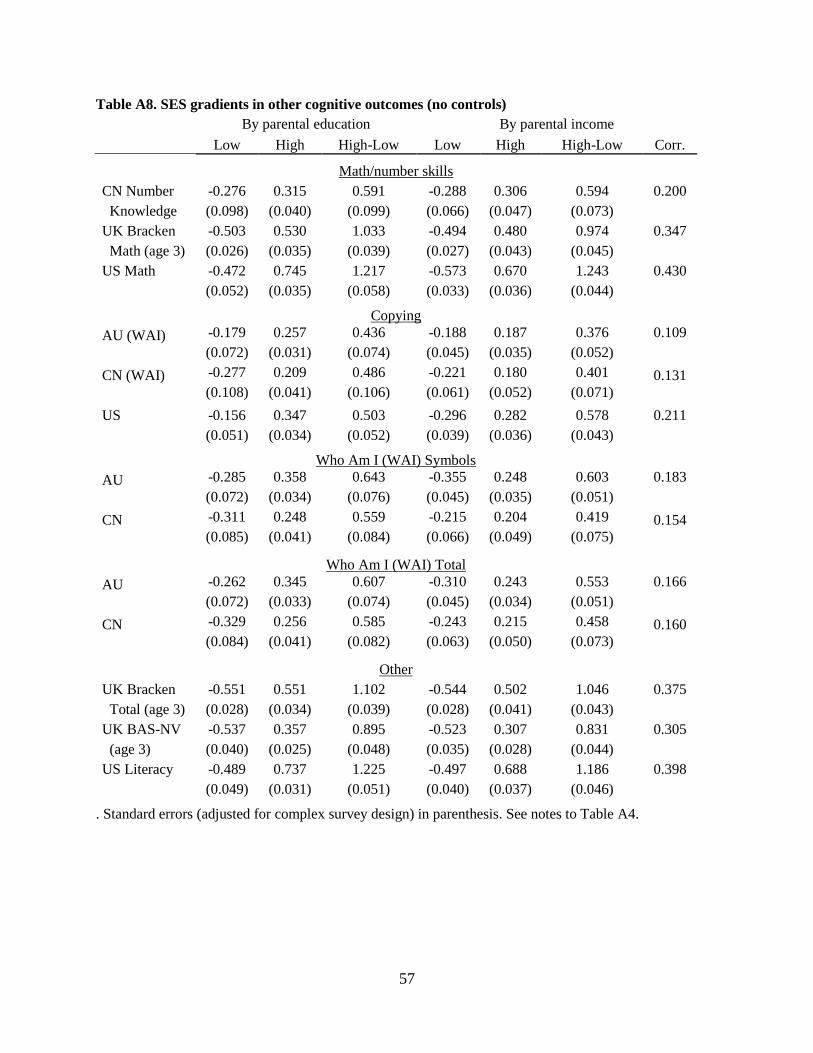
57
Table A8. SES gradients in other cognitive outcomes (no controls)
By parental education By parental income
Low High High-Low Low High High-Low Corr.
Math/number skills
CN Number -0.276 0.315 0.591 -0.288 0.306 0.594 0.200
Knowledge (0.098) (0.040) (0.099) (0.066) (0.047) (0.073)
UK Bracken -0.503 0.530 1.033 -0.494 0.480 0.974 0.347
Math (age 3) (0.026) (0.035) (0.039) (0.027) (0.043) (0.045)
US Math -0.472 0.745 1.217 -0.573 0.670 1.243 0.430
(0.052) (0.035) (0.058) (0.033) (0.036) (0.044)
Copying
AU (WAI) -0.179 0.257 0.436 -0.188 0.187 0.376 0.109
(0.072) (0.031) (0.074) (0.045) (0.035) (0.052)
CN (WAI) -0.277 0.209 0.486 -0.221 0.180 0.401 0.131
(0.108) (0.041) (0.106) (0.061) (0.052) (0.071)
US -0.156 0.347 0.503 -0.296 0.282 0.578 0.211
(0.051) (0.034) (0.052) (0.039) (0.036) (0.043)
Who Am I (WAI) Symbols
AU -0.285 0.358 0.643 -0.355 0.248 0.603 0.183
(0.072) (0.034) (0.076) (0.045) (0.035) (0.051)
CN -0.311 0.248 0.559 -0.215 0.204 0.419 0.154
(0.085) (0.041) (0.084) (0.066) (0.049) (0.075)
Who Am I (WAI) Total
AU -0.262 0.345 0.607 -0.310 0.243 0.553 0.166
(0.072) (0.033) (0.074) (0.045) (0.034) (0.051)
CN -0.329 0.256 0.585 -0.243 0.215 0.458 0.160
(0.084) (0.041) (0.082) (0.063) (0.050) (0.073)
Other
UK Bracken -0.551 0.551 1.102 -0.544 0.502 1.046 0.375
Total (age 3) (0.028) (0.034) (0.039) (0.028) (0.041) (0.043)
UK BAS-NV -0.537 0.357 0.895 -0.523 0.307 0.831 0.305
(age 3) (0.040) (0.025) (0.048) (0.035) (0.028) (0.044)
US Literacy -0.489 0.737 1.225 -0.497 0.688 1.186 0.398
(0.049) (0.031) (0.051) (0.040) (0.037) (0.046)
. Standard errors (adjusted for complex survey design) in parenthesis. See notes to Table A4.
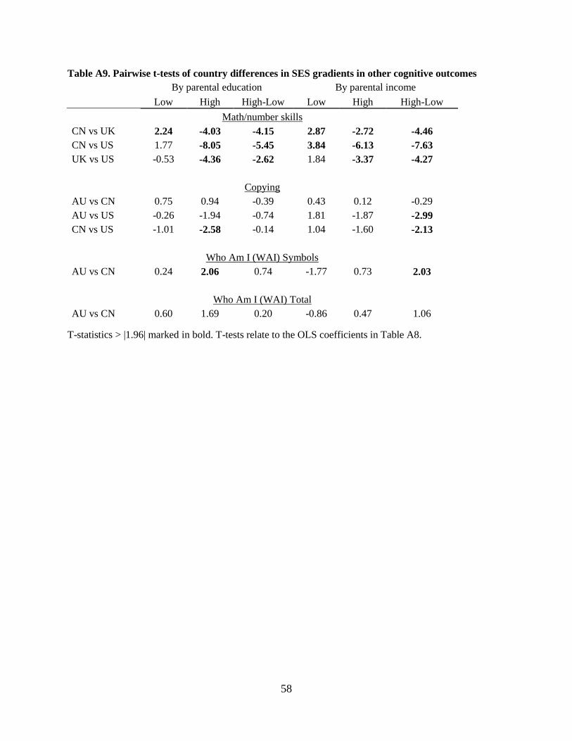
58
Table A9. Pairwise t-tests of country differences in SES gradients in other cognitive outcomes
By parental education By parental income
Low High High-Low Low High High-Low
Math/number skills
CN vs UK 2.24 -4.03 -4.15 2.87 -2.72 -4.46
CN vs US 1.77 -8.05 -5.45 3.84 -6.13 -7.63
UK vs US -0.53 -4.36 -2.62 1.84 -3.37 -4.27
Copying
AU vs CN 0.75 0.94 -0.39 0.43 0.12 -0.29
AU vs US -0.26 -1.94 -0.74 1.81 -1.87 -2.99
CN vs US -1.01 -2.58 -0.14 1.04 -1.60 -2.13
Who Am I (WAI) Symbols
AU vs CN 0.24 2.06 0.74 -1.77 0.73 2.03
Who Am I (WAI) Total
AU vs CN 0.60 1.69 0.20 -0.86 0.47 1.06
T-statistics > |1.96| marked in bold. T-tests relate to the OLS coefficients in Table A8.
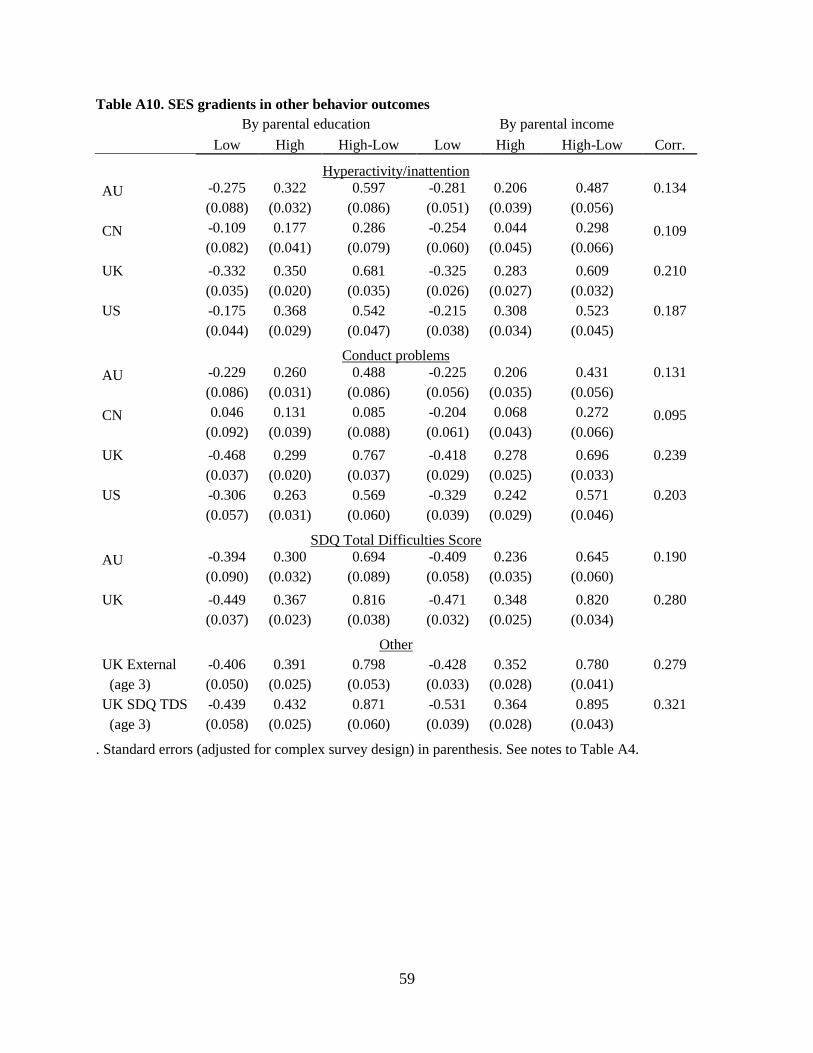
59
Table A10. SES gradients in other behavior outcomes
By parental education By parental income
Low High High-Low Low High High-Low Corr.
Hyperactivity/inattention
AU -0.275 0.322 0.597 -0.281 0.206 0.487 0.134
(0.088) (0.032) (0.086) (0.051) (0.039) (0.056)
CN -0.109 0.177 0.286 -0.254 0.044 0.298 0.109
(0.082) (0.041) (0.079) (0.060) (0.045) (0.066)
UK -0.332 0.350 0.681 -0.325 0.283 0.609 0.210
(0.035) (0.020) (0.035) (0.026) (0.027) (0.032)
US -0.175 0.368 0.542 -0.215 0.308 0.523 0.187
(0.044) (0.029) (0.047) (0.038) (0.034) (0.045)
Conduct problems
AU -0.229 0.260 0.488 -0.225 0.206 0.431 0.131
(0.086) (0.031) (0.086) (0.056) (0.035) (0.056)
CN 0.046 0.131 0.085 -0.204 0.068 0.272 0.095
(0.092) (0.039) (0.088) (0.061) (0.043) (0.066)
UK -0.468 0.299 0.767 -0.418 0.278 0.696 0.239
(0.037) (0.020) (0.037) (0.029) (0.025) (0.033)
US -0.306 0.263 0.569 -0.329 0.242 0.571 0.203
(0.057) (0.031) (0.060) (0.039) (0.029) (0.046)
SDQ Total Difficulties Score
AU -0.394 0.300 0.694 -0.409 0.236 0.645 0.190
(0.090) (0.032) (0.089) (0.058) (0.035) (0.060)
UK -0.449 0.367 0.816 -0.471 0.348 0.820 0.280
(0.037) (0.023) (0.038) (0.032) (0.025) (0.034)
Other
UK External -0.406 0.391 0.798 -0.428 0.352 0.780 0.279
(age 3) (0.050) (0.025) (0.053) (0.033) (0.028) (0.041)
UK SDQ TDS -0.439 0.432 0.871 -0.531 0.364 0.895 0.321
(age 3) (0.058) (0.025) (0.060) (0.039) (0.028) (0.043)
. Standard errors (adjusted for complex survey design) in parenthesis. See notes to Table A4.
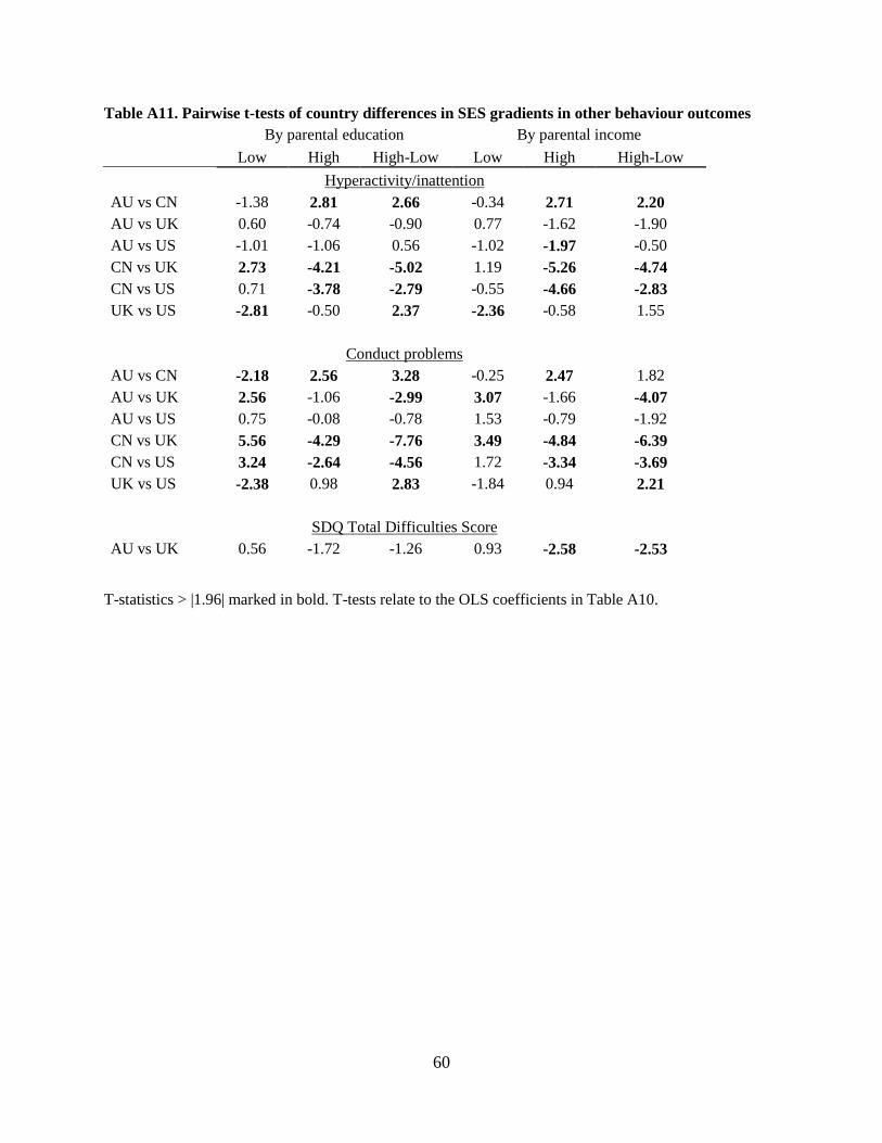
60
Table A11. Pairwise t-tests of country differences in SES gradients in other behaviour outcomes
By parental education By parental income
Low High High-Low Low High High-Low
Hyperactivity/inattention
AU vs CN -1.38 2.81 2.66 -0.34 2.71 2.20
AU vs UK 0.60 -0.74 -0.90 0.77 -1.62 -1.90
AU vs US -1.01 -1.06 0.56 -1.02 -1.97 -0.50
CN vs UK 2.73 -4.21 -5.02 1.19 -5.26 -4.74
CN vs US 0.71 -3.78 -2.79 -0.55 -4.66 -2.83
UK vs US -2.81 -0.50 2.37 -2.36 -0.58 1.55
Conduct problems
AU vs CN -2.18 2.56 3.28 -0.25 2.47 1.82
AU vs UK 2.56 -1.06 -2.99 3.07 -1.66 -4.07
AU vs US 0.75 -0.08 -0.78 1.53 -0.79 -1.92
CN vs UK 5.56 -4.29 -7.76 3.49 -4.84 -6.39
CN vs US 3.24 -2.64 -4.56 1.72 -3.34 -3.69
UK vs US -2.38 0.98 2.83 -1.84 0.94 2.21
SDQ Total Difficulties Score
AU vs UK 0.56 -1.72 -1.26 0.93 -2.58 -2.53
T-statistics > |1.96| marked in bold. T-tests relate to the OLS coefficients in Table A10.
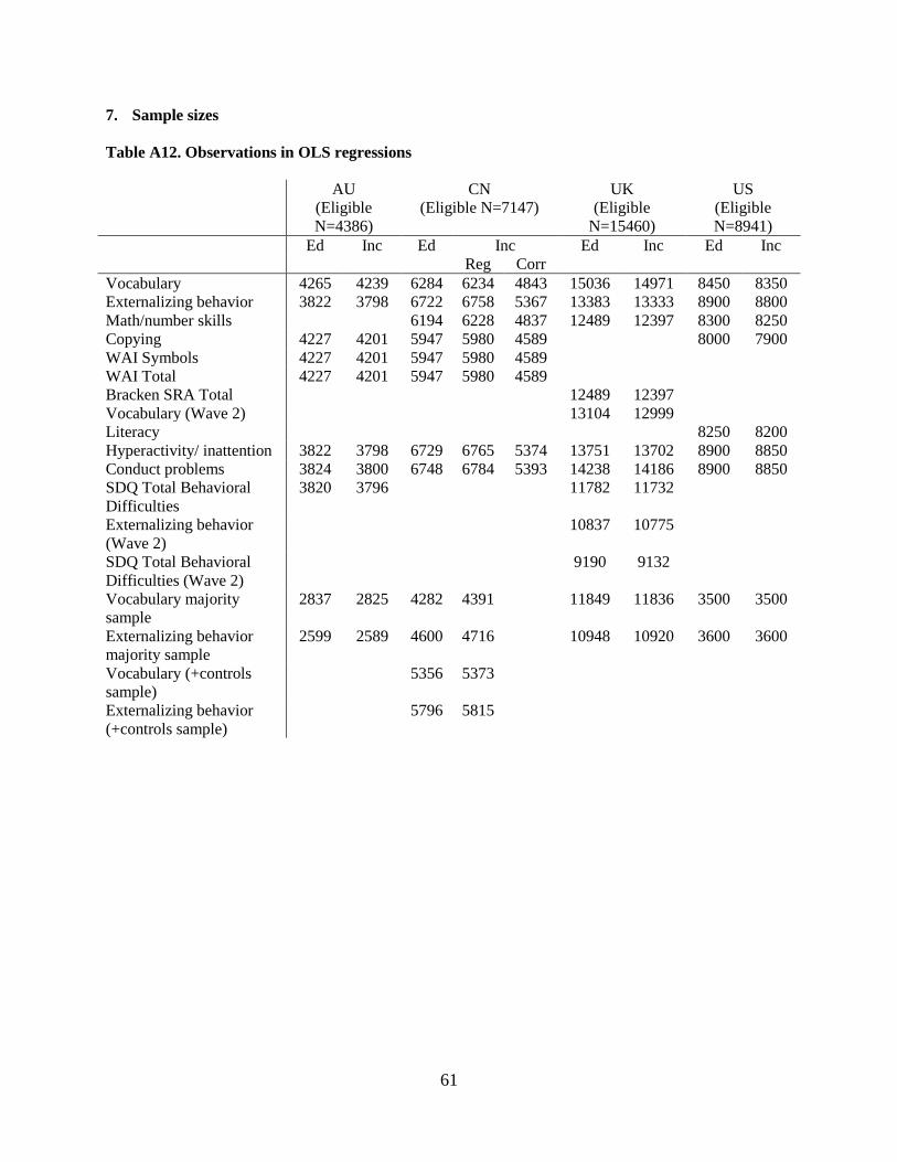
61
7. Sample sizes
Table A12. Observations in OLS regressions
AU
(Eligible
N=4386)
CN
(Eligible N=7147)
UK
(Eligible
N=15460)
US
(Eligible
N=8941)
Ed Inc Ed Inc Ed Inc Ed Inc
Reg Corr
Vocabulary 4265 4239 6284 6234 4843 15036 14971 8450 8350
Externalizing behavior 3822 3798 6722 6758 5367 13383 13333 8900 8800
Math/number skills 6194 6228 4837 12489 12397 8300 8250
Copying 4227 4201 5947 5980 4589 8000 7900
WAI Symbols 4227 4201 5947 5980 4589
WAI Total 4227 4201 5947 5980 4589
Bracken SRA Total 12489 12397
Vocabulary (Wave 2) 13104 12999
Literacy 8250 8200
Hyperactivity/ inattention 3822 3798 6729 6765 5374 13751 13702 8900 8850
Conduct problems 3824 3800 6748 6784 5393 14238 14186 8900 8850
SDQ Total Behavioral
Difficulties
3820 3796 11782 11732
Externalizing behavior
(Wave 2)
10837 10775
SDQ Total Behavioral
Difficulties (Wave 2)
9190 9132
Vocabulary majority
sample
2837 2825 4282 4391 11849 11836 3500 3500
Externalizing behavior
majority sample
2599 2589 4600 4716 10948 10920 3600 3600
Vocabulary (+controls
sample)
5356 5373
Externalizing behavior
(+controls sample)
5796 5815