Inequality, Aspirations, and Social Comparisons∗

Jonathan Bendor

Stanford University

Daniel Diermeier

Northwestern University

Michael M. Ting

Columbia University

(corresponding author)

July 2015

We develop a model of adaptive learning with social comparisons. Actors are more likely

to choose actions that recently yielded satisfactory payoffs; satisfaction is evaluated relative

to an aspiration level that reflects previous payoffs and possibly other players’ payoffs. This

captures the phenomenon of social comparison via reference groups. We show that if agents

compare themselves to those who are receiving higher payoffs then in stable outcomes all

payoffs must be equal. If, however, agents’ aspirations are driven by less ambitious social

comparisons then very unequal distributions can be stable. We apply our general results

to collective action problems in socio-political hierarchies and derive conditions for stable

exploitation. Finally, we develop a computational model which shows that increases in

payoff-inequality make outcomes less stable.

∗An earlier version of this paper was presented at the 2007 annual meeting of the American PoliticalScience Association. We thank Michael Harrison and David Kreps for helpful discussions about nonstationaryMarkov chains, and Greg Martin and Holke Brammer for their research assistance.

1

I. Introduction

When the “Occupy Wall Street” movement began in September of 2011, it quickly adopted

the slogan “We are the 99%” expressing outrage over the massive inequality in the United

States and elsewhere (e.g. Stiglitz 2011). The explicit comparison between the income and

wealth enjoyed by a tiny minority compared to the vast majority provided the emotional

fuel that launched wide-spread protests in the United States and elsewhere.

In the case of the Occupy movements economic inequality appeared to trigger wide-spread

collective action on a global scale. Yet, in other cases even more extreme social and economic

disparities are sustained over long-time periods without protests or rebellions. Political

scientists, especially Gurr (1970), have pointed to psychological mechanisms such as relative

deprivation as potential explanations for the occurrence and timing of political protests.

According to this view, revolts and rebellions are rooted in the perceived discrepancy between

an individual’s standing in society and her aspirations, resulting in anger, discontent, and

ultimately protest or violent action.1

While these explanations are certainly plausible, they are largely developed in isolation

from strategic considerations such as selective incentives (Olson 1971 [1965]) or community

enforcement (Ostrom 1990) that have dominated the analysis of collective action in the

rational choice tradition. In this paper we analyze the consequences of psychological mech-

anisms based on social comparisons in the context of strategic interaction as captured by

game-theoretic models.

In contrast to classical game theory, however, agents in our model are not fully rational.

Rather, in our model, actors adapt via aspiration-based processes: they are more likely

to choose an action if it yielded a satisfactory payoff in the preceding period, and less

likely otherwise. (Psychologists call this reinforcement learning.) A payoff is satisfactory

if it exceeds the agent’s aspiration level. Aspiration levels, however, are not fixed; they

are functions of other agents’ payoffs (Bendor, Diermeier, and Ting 2007b, Cui, Zhai, and

Liu 2009). In brief, agents observe the payoffs of others in their reference group, compare

their payoff to that reference payoff and then interpret their own payoff as satisfactory or

unsatisfactory.2 Note that agents do not form explicit expectations about the actions of

1See also Gurney and Tierney (1982).2In related work, aspirations adapt endogenously to a player’s experience, so that receiving a high payoff

2

other players in choosing their own actions; instead, they respond to positive and negative

feedback based on social comparisons.3

Social psychologists have long argued that social comparisons are a central feature of

human life. Following the seminal work of Sherif (1936) and, especially, Festinger (1954) a

multitude of studies have shown how social comparisons influence judgments (e.g., evalua-

tion of self and others), affect, and even actions. For example, individuals assessed their own

health more positively if they compared themselves to others in poorer health (Suls, Marco,

and Tobin 1991), even if they suffered from cancer (see Van der Zee, Buunk, and Sanderman

1998) or severe cardiac problems (Helgeson and Taylor 1993). Similarly, couples expressed

more satisfaction with their relationships when they compare themselves with other cou-

ples with perceived lower satisfaction. In a recent brain imaging study Fliessbach, Weber,

Trautner, Dohmen, Sunde, Elger, and Falk (2007) provide neurophysiological evidence for

the importance of social comparison on reward processing in the human brain.

Social comparisons can also have behavioral consequences. Smokers were more likely to

quit if they associated themselves with other smokers who were more able to quit (Gerrard,

Gibbons, Lane, and Stock 2005). High school students who compared themselves to peers

who out-performed them improved their grades more than others who did not (Blanton, Bu-

unk, Gibbons, and Kuyper 1999). Individual spending decisions and self-reported happiness

depend on relative comparisons of income (Veenhoven 1991, Karlsson, Dellgran, Klingander,

and Garling 2004, Luttmer 2005, Clark, Frijters, and Shields 2008, Caporale, Georgellis,

Tsitsianis, and Yin 2009). In political domains voters evaluate incumbents based on relative

increases the threshold required for satisfaction. This approach, in which aspirations adjust purely individ-ualistically, has been fruitfully used in several contexts to examine long-run behavior in normal form gamesincluding voting and turnout (e.g., Bendor, Diermeier, and Ting 2003, Bendor, Diermeier, Siegel, and Ting2011).

3Game-theorists, of course, have long noted that behavior in strategic interactions can be influenced bycommunity relationships (e.g. Ostrom 1990, Kandori 1992), but their approach is rather different. Theidea is that players may change their behavior as members of a group – for example they may cooperateeven in a single-shot prisoners’ dilemma – because defection would trigger collective punishment by theplayers’ communities. In these settings, equilibrium behavior is grounded in mutually consistent, rationalexpectations about the strategies of other players. These models not only show how cooperation can besustained endogenously, they also help identify some of the factors that may promote or hinder cooperativebehavior. For example, an interesting feature of these models is that all else equal, the density and structureof communal interaction makes contingent punishments more severe, thus better deterring defection (Bendorand Mookherjee 1990, Kandori 1992). However, although these approaches are insightful, from a behavioralperspective they are somewhat problematic as the proposed mechanisms for cooperation depend on precisecoordination on a particular punishment protocol, a demanding task especially in large groups.

3

comparisons of economic performance (Kayser and Peress 2012).

Social structures such as reference groups are conveniently modeled as networks (e.g.

Jackson 2008). In the context of social comparisons, for example, individual i may compare

herself to individual j by tracking j’s payoff. Social comparisons may not be symmetric.

That is, i may track j, but j may pay no attention to i. To capture different strengths of

influence we will use influence matrices that assign different weights to different comparisons.

While social influence networks are often exogenous, they may also change over-time either

randomly or in response to received payoffs (e.g. Lazer, Rubineau, Chetkovich, Katz, and

Neblo 2010). In our model we allow for influence structures that change over time.

Our model examines the impact of such comparisons on collective choice contexts. We

represent these interactions as non-cooperative games. We proceed in three steps. First,

we establish some general characteristics of adaptation under social comparisons. These

results hold for any strategic interaction modeled as a repeated normal form game. They

identify network properties of social comparison that determine whether stable outcomes

require equal payoffs for all players. Thus, they are especially relevant to a classical problem

in political sociology: the stability of inequality (e.g., Runciman 1966).

Second, we apply these results to two important types of collective action problems:

public goods and resource-allocation. This allows us to probe what stabilizes hierarchies.

Our main results establish that the stability of unequal distributions depends on a key feature

of social comparisons. If agents compare themselves only with agents with the same or lower

payoffs, inequality can be stable. If, however, they “look up”—their aspirations are driven

by the perception of people who are doing better than they are—then inequality is unstable.

Finally, we use computational methods to do two things: check the robustness of the

analytical model and “smooth it out,” i.e., allow us to examine the degree of instability of

different outcomes (and hence of different systems). Fortunately, these two tasks complement

each other: once we have done the latter, doing the former turns out to be easy. Proceeding

in this way, we find that our main results (properly understood) are robust: inequality tends

to destabilize outcomes.

4

II. The Model

Basic Concepts and Notation

Throughout the paper we assume infinitely repeated normal form games, with fixed stage

games and deterministic payoffs. Let t denote discrete time periods and i denote actors

(i = 1, . . . , n), with n finite. Each player i has mi > 1 actions, where mi is finite. Player

i’s generic action is denoted αi. An outcome o corresponds to an element in the associated

normal form payoff matrix. We write α(o) to denote the action profile that generates outcome

o and αi(o) to denote i’s action within that profile.

A player’s probability of playing action αi at t is denoted pi,t(αi). Similarly, pi,t is i’s

probability distribution over all actions at t. Let πi,t(o) denote i’s payoff, given outcome

o. Aspiration levels are called ai,t. We assume that there is an aspiration level for each

possible payoff level, i.e. for each i, t and o there exists some ai,t such that ai,t = πi,t(o). For

convenience we will drop time subscripts when the meaning is clear.

Propensity- and Aspiration-Adjustment

Players’ propensities are governed by two similar mechanisms. At each period, every player

i becomes more likely to choose an action if it was coded as successful in the previous period.

A success for i occurs when her payoff exceeds her aspiration level. Analogously, i reduces her

likelihood of choosing any action coded as a failure. Observe that these rules are compatible

with a wide range of functional forms.

A1 (positive feedback): If i used action αi in t and if πi,t ≥ ai,t then pi,t+1(αi) ≥ pi,t(αi);

this conclusion holds strictly if pi,t(αi) < 1 and πi,t > ai,t.

A2 (negative feedback): If i used action αi in t and if πi,t < ai,t then pi,t+1(αi) ≤ pi,t(αi);

this conclusion holds strictly if pi,t(αi) > 0.

The heart of aspiration-adjustment is that aspirations respond to experience (payoffs).

In this model, agent i’s aspiration in period t+ 1 is a weighted average of his current payoff

and those of some of the other players. We call the latter i’s reference group. If player j is

in i’s reference group then we will say that i tracks j, as shorthand for “i tracks j’s payoff.”

We call this a process of social comparison. We also assume that ai,t+1 is always influenced

by i’s current aspiration, ai,t.

5

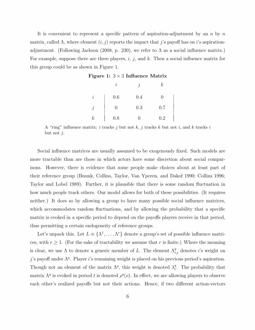
It is convenient to represent a specific pattern of aspiration-adjustment by an n by n

matrix, called Λ, where element (i, j) reports the impact that j’s payoff has on i’s aspiration-

adjustment. (Following Jackson (2008, p. 230), we refer to Λ as a social influence matrix.)

For example, suppose there are three players, i, j, and k. Then a social influence matrix for

this group could be as shown in Figure 1.

Figure 1: 3× 3 Influence Matrix

i j k

i 0.6 0.4 0

j 0 0.3 0.7

k 0.8 0 0.2

A “ring” influence matrix: i tracks j but not k, j tracks k but not i, and k tracks ibut not j.

Social influence matrices are usually assumed to be exogenously fixed. Such models are

more tractable than are those in which actors have some discretion about social compar-

isons. However, there is evidence that some people make choices about at least part of

their reference group (Buunk, Collins, Taylor, Van Yperen, and Dakof 1990; Collins 1996;

Taylor and Lobel 1989). Further, it is plausible that there is some random fluctuation in

how much people track others. Our model allows for both of these possibilities. (It requires

neither.) It does so by allowing a group to have many possible social influence matrices,

which accommodates random fluctuations, and by allowing the probability that a specific

matrix is evoked in a specific period to depend on the payoffs players receive in that period,

thus permitting a certain endogeneity of reference groups.

Let’s unpack this. Let L ≡ {Λ1, . . . ,Λr} denote a group’s set of possible influence matri-

ces, with r ≥ 1. (For the sake of tractability we assume that r is finite.) Where the meaning

is clear, we use Λ to denote a generic member of L. The element Λqi,j denotes i’s weight on

j’s payoff under Λq. Player i’s remaining weight is placed on his previous period’s aspiration.

Though not an element of the matrix Λq, this weight is denoted λqi . The probability that

matrix Λq is evoked in period t is denoted ρq(o). In effect, we are allowing players to observe

each other’s realized payoffs but not their actions. Hence, if two different action-vectors

6

produce the same vector of payoffs then they generate the same probability distribution over

L.

We can see how this setup allows for endogenous reference groups by re-examining the

above three-person example. Suppose player j is ambitious, in the sense of only tracking

players who receive higher payoffs than he does in any given period. Suppose in outcome o1

the payoffs are πi(o1) > πj(o1) > πk(o1) whereas in outcome o2 they are πi(o2) < πj(o2) <

πk(o2). If o1 happens in t, then the probability that j tracks k in t is zero, whereas if o2

occurs then the chance that j tracks i in t would be zero. Formally, this would be represented

by the probability distribution of ρq(·), which conditions on the realized payoff vector. If

this distribution is the same for all possible payoff vectors, then we recover the simple case

of exogenously fixed social influence. (Note, however, that even this simple case allows for

random fluctuations in who tracks whom.)

These social influence matrices and their associated probabilities may reflect some in-

terdependence among players’ reference groups. For example, suppose i and j form a tight

subgroup, so Λi,j > 0 and Λj,i > 0 in every Λ in L. Hence their tracking of k may not be inde-

pendent: roughly speaking, Pr(Λi,j > 0 and Λj,i > 0) could exceed Pr(Λi,j > 0) ·Pr(Λj,i > 0).

(Indeed, it may be that for every Λ ∈ L player k is either in the reference groups of both i

and j or she is in neither reference group; the mixed cases never occur.)

A3 summarizes the assumptions about aspiration-adjustment.

A3 (aspiration adjustment):

(i) There are r ≥ 1 n × n social influence matrices, labeled Λq (1 ≤ q ≤ r). The

probabilities ρq(o) of selecting Λq are fixed and independent over time but may depend on

o, the realized vector of payoffs.

(ii) For any realized social influence matrix Λq, the weights Λqi,j are non-negative and on

each row i (i = 1, . . . , n) sum to 1− λqi , where λqi ∈ (0, 1) is the weight on ai,t in Λq.

(iii) For any realized social influence matrix Λq, ai,t+1 = λqiai,t +∑n

j=1 Λqi,jπj,t.

Note that A3 allows for the possibility that some players adjust their aspirations in a

purely individualistic way. This occurs for player i when λqi + Λqi,i = 1 for all Λq ∈ L.

It is worth emphasizing that players in our model are not imitating each other’s ac-

tions. Instead, what social comparisons directly impact is a cognitive variable: aspiration

7

levels. Thus, our model combines key features of two lines of network research that have

remained mostly disjoint: models in which players imitate actions (Jackson 2008, chapter

9) and those which focus on the diffusion of opinions, information, and other cognitive vari-

ables (Jackson, chapter 8). The former are often ‘behaviorist’: they may not represent any

cognitive variables at all. The latter are often purely cognitive: the agents may not take

any actions; everything—e.g., opinion-change—happens inside their heads. In our model, a

cognitive variable (aspirations) and an associated adaptive rule drive behavior. Actions in

turn generate payoffs which impact the cognitive variable, and ’round it goes.

Note that our model defines a stochastic process, with states that are sets of action-

propensities and aspirations. The best-understood kinds of stochastic processes are Markovian—

tomorrow’s probability distribution over the possible states depends only on today’s state

and the transition rules—with stationary (time-homogeneous) transition rules. Fortunately,

however, few of our results require these properties.

Of course, imposing special structure usually boosts a model’s predictive power, so in

Section V (and occasionally elsewhere) we will exploit the added power conferred by assuming

that the stochastic process is both Markovian and stationary. Indeed, we will soon see that

thinking about these special types of stochastic processes helps to give us intuitions about

what kinds of outcomes we should expect to see and which we should not.

First, however, we must examine the primitives of our process—action-propensities and

aspirations—and the implications of our basic axioms, A1-A3. Intuitively, if the process

settles down on some of these states then it probably also settles down on their observable

products: actions and outcomes. Hence it makes sense to look for states with self-replicating

properties. This idea is expressed in Macy and Flache’s notion (2002) of a self-reinforcing

equilibrium with endogenous aspirations where both aspirations and propensities are fixed

points. Here we focus on a generalization of their solution concept. In this generalization, the

propensities must be self-replicating. Specific aspiration-values need not, however, replicate

themselves, i.e. they do not need to be fixed points. (This is useful because reference groups

and hence aspirations can change over time.) Instead, we require only that there exists a set

of aspirations that (a) is absorbing—once aspirations enter the set they never leave it—and

(b) as long as aspirations stay in that set then propensities replicate the required specific

values. (Of course, a singleton set can satisfy these properties.) Formally,

8

Definition 1 A Self-Reinforcing Equilibrium (SRE) is a vector of propensities (pi,t)i

and a compact set of aspirations Ai satisfying ai,t ∈ Ai for each i, where for all i, αi, and

t′ > t:

(i) pi,t′(αi) = pi,t(αi),

(ii) ai,t′ ∈ Ai.

SREs do not exist in all games, even for stationary Markovian processes. Consider the

example in Figure 2. In this example no outcome is stable in the above sense if both players

track each other. However, the absence of stable outcomes does not mean that the model

makes no prediction. It means only that the process does not in the limit get absorbed

into an outcome. Instead, the process will exhibit more complicated dynamics: individual

sample paths never settle down.4 (As we will see in section V, if the sample paths produced

by players interacting in the game of Figure 2 are produced by a stationary Markov process

then under plausible conditions the process will produce a stable distribution of outcomes.)

Figure 2: No Stable Outcome

C D

C 701, 700 0, 900

D 900, 0 400, 401

4For stationary Markov processes there is a strong connection between self-replicating equilibria (SRE)and an intuitive notion of a stable outcome. Imagine agents adapting by adjustment rules that accord withA1-A3. Clearly, if the associated process gets absorbed into outcome o—if it reaches o it stays there—thenwe would naturally say that o is stable. We will see later that if a process is Markovian and stationary andis not shocked by random perturbations then an outcome is stable in this sense if and only if it is supportedby self-replicating propensities and aspirations. (As we will see, outcomes that are not supported by SREscan be unstable in a very basic sense. Not only are they not absorbing; they may be transient : eventuallythe process will leave them and never return. For example, if two agents are playing a standard prisoner’sdilemma and their adjustment rules create a stationary Markov process then the asymmetric outcomes of(defect, cooperate) and (cooperate, defect) will be transient if both players engage in social comparisons.)In section V we will analyze stochastic processes that are perturbed by random shocks. We will sometimeslean on this intuitive notion of stability and tersely refer to ‘stable outcomes’ as shorthand for ‘outcomesthat are supported by SREs, under certain types of stochastic processes’.

9

III. General Results

We now investigate how the structure of social comparison determines whether unequal

outcomes are stable. The topic of stable hierarchies is, of course, a venerable one in political

sociology, going back to Marx and de Tocqueville.

We show that there are two distinct forces underlying social comparison that link stability

and equality. One is the sheer availability of information about how other people are doing.

In many contemporary societies, it can be hard to avoid social comparisons: modern media

regularly put them before us. This factor is exogenous in our model. The other force is partly

endogenous reference groups, produced by the proclivities of people tantalized by those who

are doing better than they are. We take these up in turn.

Exogenously Dense Social Comparisons

Our first set of general results turn on a key network property concerning the density of

reference groups among a set of players. This property is probabilistic: it allows for different

social comparisons (different Λ’s) to hold at various dates. In order to explain this concept

clearly, it is helpful to first introduce a simpler, deterministic notion that is a special case of

ours.

Let’s reconsider the social influence matrix of Figure 1. This is a ring structure: i tracks

j, j tracks k, and k tracks i. We will call this a strongly connected network or structure.5

As the term suggests, a strongly connected system cannot be broken up into self-contained

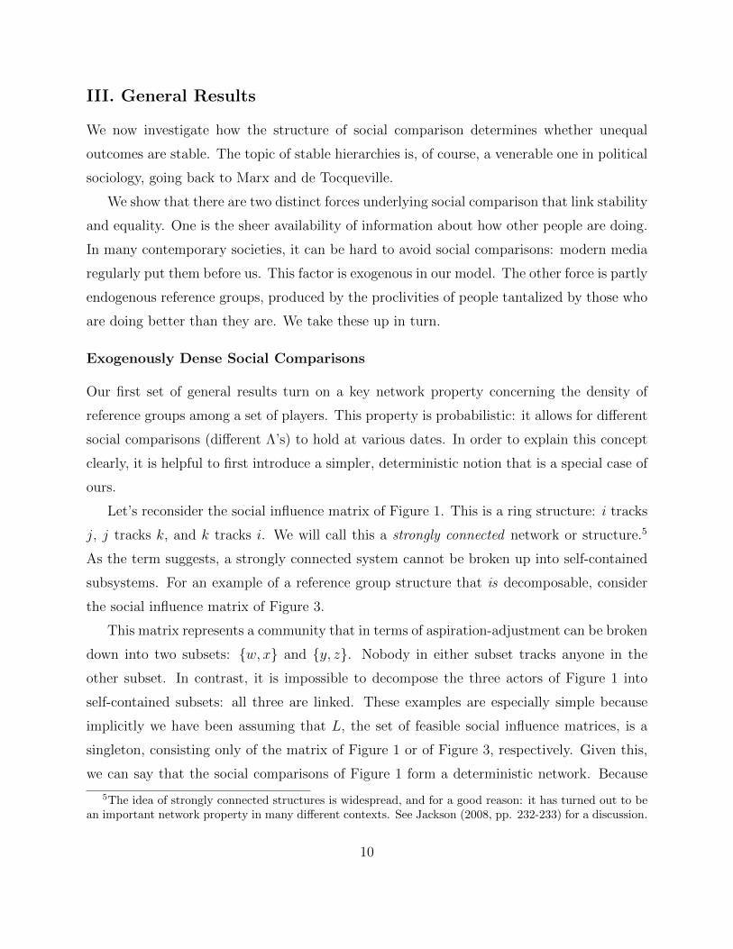
subsystems. For an example of a reference group structure that is decomposable, consider

the social influence matrix of Figure 3.

This matrix represents a community that in terms of aspiration-adjustment can be broken

down into two subsets: {w, x} and {y, z}. Nobody in either subset tracks anyone in the

other subset. In contrast, it is impossible to decompose the three actors of Figure 1 into

self-contained subsets: all three are linked. These examples are especially simple because

implicitly we have been assuming that L, the set of feasible social influence matrices, is a

singleton, consisting only of the matrix of Figure 1 or of Figure 3, respectively. Given this,

we can say that the social comparisons of Figure 1 form a deterministic network. Because

5The idea of strongly connected structures is widespread, and for a good reason: it has turned out to bean important network property in many different contexts. See Jackson (2008, pp. 232-233) for a discussion.

10

Figure 3: 4× 4 Influence Matrix

w x y z

w 0.6 0.4 0 0

x 0.7 0.3 0 0

y 0 0 0.2 0.8

z 0 0 0.5 0.5

A decomposable influence matrix: w and x track only each other, and y and z trackonly each other.

the model of the present paper allows for randomness in reference groups—different social

influence matrices can occur in different periods—we use a probabilistic notion of relatedness.

Informally, a set of players are probabilistically strongly connected if, for every partition of

the set into two disjoint, nonempty subsets, there’s a chance—not necessarily a certainty—

that at least one person in each subset tracks someone in the other subset. This idea is

formalized below.

Definition 2 Set N is (probabilistically) strongly connected if, for every J ⊂ N , where

J 6= ∅ and J 6= N , there exists some j ∈ J and i ∈ N\J and some Λq ∈ L such that Λqj,i > 0

and there exists some i′ ∈ N\J and j′ ∈ J and some Λq′ ∈ L such that Λq′

i′j′ > 0.

If a network of social comparisons is deterministically strongly connected then of course

it must be probabilistically so as well. (It is easy to check, for instance, that the matrix of

Figure 1 satisfies Definition 2.) But the converse does not hold: the players could form a

probabilistically strongly connected system even if no feasible social influence matrix satisfies

Definition 2 by itself. For example, suppose that there are three feasible Λ’s for some three-

person group. In Λ1, the only social comparison is that i tracks j; in Λ2, only j tracks k; in

Λ3, just k tracks i. Although any particular reference group structure is decomposable, the

set of players is probabilistically strongly connected.

Henceforth, we will simply say that a set of players is strongly connected, as shorthand

for saying that it is probabilistically strongly connected in the sense of Definition 2.

11

Our first result shows that if reference groups are dense enough to create a strongly

connected community then outcomes with heterogeneous payoffs will not be tolerated: they

are unstable. (The proofs of Theorem 1 and of most of the other results are in the appendix.)

Theorem 1 If the set of players is strongly connected then an outcome is supported by a

self-reinforcing equilibrium if and only if that outcome gives all players the same payoff.

Theorem 1 yields the following corollary. (The proof, being straightforward, is omitted.)

Suppose we restrict attention to aspiration-based adaptive rules that are Markovian and

stationary. In this context, Theorem 1 implies that if payoffs are heterogeneous in every

outcome then no outcome is stable. This corollary tells what will not happen but not what

will. What, then, should we expect to occur in such circumstances? We will return to this

question in Section V.

Strongly connected social comparison networks produce a drive toward equality for a

simple but powerful reason: such systems are dense enough to ensure that some people on

the bottom of a hierarchy track some people who are doing better than they are. To see this

in a stark setting, consider a community divided into two groups: haves and have-nots—A’s

and B’s, respectively. All A’s get the same payoff, πA; all B’s get πB < πA. Suppose B’s

tracked only each other. Then in the steady state their aspirations would equal πB, whence

they would be content with their lot. Therefore, this outcome can be stabilized by some

self-enforcing equilibrium. (It does not matter whom A’s track: they will be satisfied in

any network of social comparisons.) But if B’s track only each other then the system is not

strongly connected: if the community is partitioned into A’s and B’s then with probability

one nobody in the latter tracks anyone in the former, which violates Definition 2. If the

system were strongly connected then at least one B would sometimes track an A. But if that

happened then that B’s aspiration would exceed πB—and she would be dissatisfied with her

action. This would destabilize inequality.

The logic of this simple example holds generally.

Proposition 1: An outcome with unequal payoffs is supported by a self-enforcing equi-

librium only if there is no Λ such that an agent with the minimum payoff tracks any agent

receiving more than the minimum payoff, i.e., only if nobody at the bottom tracks anyone

higher.

12

Strong connectedness ensures that the condition described by Proposition 1 cannot hold.

And since this condition of nobody at the bottom tracking anyone higher is necessary for

inequality, strong connectedness is sufficient for equality.

We next explore inequality, when Proposition 1’s condition does hold.

Partially Decomposable Communities

We call a group of players closed if nobody in the group tracks anyone outside it, under any

matrix in L.

Theorem 2 If the players can be partitioned into k disjoint nonempty groups, A1, . . . , Ak

(1 < k < n) such that each group is strongly connected and l of the groups (1 ≤ l ≤ k),

A1, . . . , Al, are closed, then the following conclusions hold.

(i) An outcome can be supported by a self-reinforcing equilibrium only if all payoffs in

group Aq are the same, for all q = 1, . . . , l.

(ii) If all k groups are closed (i.e., l = k) then homogeneous within-group payoffs is also

sufficient for the conclusion of (i).

The exogenous reference group structure of Theorem 2 permits the existence of stable

payoff-inequalities.6 We will explore the impact of endogenous reference groups in the next

section.

6Theorem 2 provides some methodological insight regarding the empirical content of aspiration-basedmodels of adaptation. Bendor, Diermeier and Ting (2007a) show that for a wide class of aspiration-basedadaptive rules any outcome of the stage game can be sustained as a stable outcome by some pure self-replicating equilibrium. (A pure self-replicating equilibrium is one in which the vector of propensities (pi,t)iis degenerate: for each player i, pi,t(αi) = 1 for some αi and pi,t(α

′i) = 0 for all other actions α′i.) Intuitively,

this means that such models lack empirical content as they are consistent with any observable behavior,similar to the well-known folk-theorems in non-cooperative game theory. Although the folk theorems ofBendor, Diermeier and Ting (2007a) are more general in some respects than the present paper’s Theorem2, in one respect they are more specialized: they are equivalent to the case of k = n groups: every player isan island (regarding aspiration-formation). More generally, the empirical content of the model is decreasingin k, the number of reference groups. If k = 1, what can happen (stably) is tightly constrained. If k = n,anything can be a stable outcome. The degree of constraint falls monotonically as k increases from 1 to n.

13

Endogenous Reference Groups

Now we analyze social comparisons that are influenced by realized outcomes. Players, know-

ing these outcomes, can compare themselves to people who are doing better than they or to

those doing worse.

In the following results, π(o) denotes the highest payoff that any player gets in outcome

o, while π(o) is the lowest.

Definition 3 Social comparisons are based on looking upwards if the following condition

holds for all outcomes: if πi(o) < π(o) for player i in outcome o, then given o player i tracks

j only if πj(o) > πi(o).

Theorem 3 If social comparisons are based on looking upwards and for every i and every

o there is a Λq(o) ∈ L such that λqi (o) + Λqi,i(o) < 1 then an outcome is supported by a

self-reinforcing equilibrium if and only if that outcome gives all players the same payoff.

As Runciman and other political sociologists have argued, looking up creates a drive

toward equality.7 Note that social comparisons may be based on looking upwards yet not

produce a strongly connected network. For example, suppose that we are investigating

the stability of outcome o, which yields different payoffs for all agents. (For convenience,

number the players so that π1(o) > · · · > πn(o).) Assume that actors 2 through n look up;

specifically, they track only player 1. Obviously these social comparisons destabilize this

outcome: the aspiration level of everyone other than player 1 is a weighted average of his

own payoff and the top value, π1(o), so dissatisfaction is rampant. But this network is not

strongly connected. (To see this, partition it into the subsets of {1} and {2, . . . , n}. Nobody

in the first subset tracks anyone in the second one (i.e., player 1 tracks no one); hence,

Definition 2’s criterion is not satisfied.8 This shows that ambitious social comparisons and

strong connectivity are different causes of the same effect.

7“[A]lthough the enjoyments of the workers have risen, the social satisfaction that they give has fallenin comparison with the increased enjoyments of the capitalist, which are inaccessible to the worker” (Marxand Engels, quoted in Davies 1962, p.5).

8In graph theory this network would be called weakly connected. The notion of weak connectivity is basedon undirected graphs. Because aspiration networks with reference groups are intrinsically directed structures,the concept of weak connectivity is less useful for present purposes than is that of strong connectivity, whichis based on directed graphs.

14

In contrast to the restlessness produced by looking up, looking down or sideways produces

contentment with the status quo (Runciman 1966).9 Hence, these kinds of social comparisons

stabilize inequality.

Definition 4 Social comparisons are based on looking downwards or sideways if the follow-

ing condition holds for all outcomes: given outcome o player i tracks j only if πi(o) ≥ πj(o).

Theorem 4 If social comparisons are based on looking downwards or sideways then

any outcome, no matter how unequal the payoffs, is supported by some self-reinforcing

equilibrium.

If some people in the community are ambitious—they look up—whereas others prefer the

self-enhancement generated by looking down or sideways, then stability requires appeasing

the ambitious.

Corollary 1 If the set of players is divided into two subsets, those who look up and those

who look down or sideways, and λqi + Λqi,i < 1 for all ambitious players in all Λq, then an

outcome o is supported by a self-reinforcing equilibrium if and only if all the ambitious agents

get π(o), the maximal payoff anyone gets in o.

The corollary points out the stabilizing force of raising the payoffs of ambitious community

members, or cooptation. If inequality is to be stable, those on top must figure out how to

co-opt those who are (1) less well off and (2) ambitious.

Another way of stating the necessity condition in Corollary 1 is as follows. Suppose

a player would look up if someone’s payoff exceeded his. Then he’d be disgruntled: his

aspiration would exceed his payoff. So that outcome would be unstable, even if all the

other players were content with their lot. Note that these results go well beyond relative

deprivation theory (Gurr 1970), which predicts that social comparisons lead to the formation

of social movements and rebellions but does not predict that the outcomes of such activities

will eventually lead to less inequality. Our model implies not only protest activity, but less

unequal social outcomes.

9As social psychological research indicates, looking down can enhance one’s sense of self (Taylor and Lobel1989, Wills 1981; however, see Collins 1996 for complications). This may be an important motive for thechoice of social comparisons.

15

To further explore these issues we investigate two specific collective choice problems: the

production of public goods and the allocation of resources.

IV. Collective Action Problems and Inequality

Viable communities must solve two vital collective action problems. First, they must pro-

duce some public goods. This usually includes security (Tilly 1992); it often includes the

protection of a commons or some other resource (Ostrom 1990). Second, they must figure

out some way to allocate resources without too much violence. Either process can produce

inequality. Some people may shirk in the production of collective goods, thus exploiting

those who work hard. In resource-allocation, some people may behave more aggressively

than others and thereby grab bigger slices of the pie. Hence, both of these critical processes

can be conflictual: those who are more pro-social may wind up with less value than those

who are less pro-social.

We represent these possibilities by a large class of games. Although the games are

symmetric in the standard sense—everyone has the same set of actions and reversing two

players’ actions reverses their payoffs—this class of games is defined by their asymmetric

outcomes. Roughly speaking, the defining property is this: if player i’s action is more pro-

social than player j’s, then the latter’s payoff exceeds the former’s.10 (Since the game is

symmetric, if the players use the same action then their payoffs are equal.) For example, the

infamous game of Chicken belongs to this class. As Figure 4 shows, if player 1 is aggressive

while player 2 is conciliatory, then the former’s payoff exceeds the latter’s. (Indeed, player 1

gets the game’s maximal payoff in this circumstance.)

We will give a precise definition of this class of games below. First we must provide

some notation and assumptions. The common action-set is {α1, . . . , αm}, with m > 1.

Without loss of generality, the actions are labeled so that lower-numbered actions are more

pro-social than higher-numbered actions. For example, cooperation in the standard binary-

choice Prisoner’s Dilemma would be α1; defection would be α2.

10So-called divide-the-dollar games do not belong to the class of conflictual games for a technical reason:if the sum of the demands exceeds a dollar (more generally, the feasible pie of value) then everyone getsexactly the same payoff—zero—no matter what their individual demands were. An ε-perturbation to thepayoffs in the required direction (more aggressive demands yield ε-higher payoffs) yields situations that dobelong to the class of games examined here.

16

Figure 4: Chicken Game

Aggressive Conciliatory

Aggressive 0, 0 3, 1

Conciliatory 1, 3 2, 2

Definition 5 A symmetric one-shot game is called conflictual if αi(o) = αr, αj(o) = αs,

and r < s for any outcome o and any players i and j, then πi(o) < πj(o).

Note that in resource-allocation contexts, aggressive agents are generally being more

active than their less aggressive brethren, whereas in public good games shirking often entails

passivity. Despite this difference, in both situations it is clear which actions are pro-social

and which are not.

We model a community of n players who are playing a conflictual game in every period.

The game may involve providing a public good or resource-allocation or any other situation

that satisfies Definition 5. Consider a community with k > 1 groups. Can these groups form

a stable hierarchy? The following pair of results address this question. Note that Corollary

2 follows from Theorem 3: given the key property of conflictual games—if two actors take

different actions then the more pro-social one gets a lower payoff—everybody will be satisfied

with an outcome only if they use the same action.

Corollary 2: Suppose that social comparisons are based on looking upwards and λqi+Λqi,i <

1 for all i and all q. If the stage game is conflictual then an outcome can be supported by

a self-reinforcing equilibrium if and only if everyone takes the same action (and hence gets

the same payoff).

The following result follows from Theorem 4. What we call higher-status groups are those

that get higher payoffs than lower status ones. Thus, the groups form a hierarchy.

Corollary 3: Suppose that social comparisons are based on looking downwards or sideways.

If the stage game is conflictual and actors have at least as many actions as there are groups,

then there exists an SRE in which the groups form a hierarchy: (1) actions within a group

17

are homogeneous and (2) actions across groups are heterogeneous, with higher status groups

behaving in a less pro-social way than lower status ones.

Finally, once again we see a connection between cooptation and stable inequality.

Corollary 4: Suppose the hypotheses of Corollary 1 hold. If the stage game is conflictual

then an outcome is supported by a self-reinforcing equilibrium only if (i) all ambitious agents

behave homogeneously and (ii) nobody behaves in a less pro-social way than the ambitious

agents.

Part (ii) of this result implies that the ambitious agents get the maximal payoff, π(o).

Our analysis shows that social reference structures where agents look downwards and

sideways can sustain unequal social hierarchies. Members of each social stratum do equally

well, but across strata behavior differs: groups of higher status take advantage of lower ones

by behaving less pro-socially, either by contributing less to public goods or by grabbing more

resources. Social hierarchies thus become self-sustaining. Lower status people end up with

less but, perhaps because of their lower status, do not compare themselves to higher status

individuals. These restrictions to downward and sideways comparisons maintain unequal

allocations in equilibrium.

V. Robustness and Degrees of Instability: A Computational Model

Thus far we have used analytical methods to investigate the relation between inequality and

instability. These approaches are powerful but they exact a price: to keep a model tractable,

assumptions often must be stated crisply—e.g., payoffs are either exactly equal or they’re

not. Further, the stability concept of self-reproducing equilibria is also crisp: either an

outcome is an SRE or it is not. Together, these two dichotomies yield a conclusion—unequal

payoffs are unstable (Theorems 1 and 3)—that is very sharp but perhaps unrealistically

so. Inequality is a matter of degree. Some payoffs, though not precisely equal, are almost

so; others are wildly divergent. As the current controversy over income inequality in the

United States indicates, the degree of inequality matters empirically. Similarly, the intuitive

hypothesis is that outcomes in the real world exhibit degrees of stability: they are not either

perfectly stable or completely unstable.

Hence it makes sense to examine the relation between inequality and instability under a

18

more nuanced set of assumptions. In this section we will investigate whether an increase in

payoff-inequality makes an outcome less stable, a continuous analog to the analytical model’s

dichotomous conclusion that unequal payoffs are unstable.

Fortunately, there are standard methods for studying degrees of stability. Probably the

best-known approach is to construct a model which has an ergodic stochastic process: (1)

there is a unique invariant probability distribution over the state space and (2) the process

converges to that unique distribution from any initial vector of probabilities over the states.

In the present context, ergodicity would ensure that there is an invariant distribution over

actions and outcomes. This in turn automatically provides a stability-metric: an outcome’s

stability is measured by a continuous variable, its limiting probability, which reflects how

long the process will dwell there in the long run. For example, consider the (stationary)

Markov chain in Figure 5.

Figure 5: 2-State Probability Transition Matrix

a b

a 0.8 0.2

b 0.7 0.3

Neither state is absorbing, so neither is perfectly stable. Clearly, however, state a is more

stable than b: the process is likely to leave the latter but not the former. This difference is

reflected in the states’ limiting probabilies: a’s is 79; b’s, only 2

9.

There are several ways to ensure that our process is ergodic for a large class of n-person

games. A convenient standard approach is to introduce shocks to action-propensities: at

any date an agent might move to a propensity vector that is totally mixed over his set of

actions. Thus, with a possibly small probability, an agent does not do what she intends to

do. The shocks to action-propensities are independent across players and i.i.d. for a given

agent. (For technical reasons one also must ensure that the process is aperiodic, i.e., does not

mechanically alternate between states. This is easily accomplished by introducing a small

amount of inertia into the adjustment processes, which is what we do here.)

Because it is difficult to solve this model analytically, i.e., to generate closed-form results,

we mostly use computational methods. (At the end of this section we examine a special case

19

that is tractable enough to allow us to return to analytical methods.) The computational

model, which we describe below, can address robustness questions by generating numerical

output regarding the limiting distribution.11

To reduce computing time we study the simplest possible strategic contexts, 2×2 games.

For the adjustment of action-propensities we use the standard Bush-Mosteller rule, a cor-

nerstone of many models of learning and adaptive behavior.12 Adjustment in this rule is a

linear function of the amount of available propensity. For example, suppose that an agent

has two actions, cooperate (C) or defect (D), and she tries C in t and it yields a satisfactory

payoff (i.e., positive feedback). Then

pC,t+1 = pC,t + θ(1− pC,t), (1)

where θ, a constant in (0, 1], is the speed of adjustment. An analogous equation holds for

negative feedback.

The agents update their aspirations each round according to a simple weighted average

rule. For example, for agent 1 the rule is as follows:

a1,t+1 = (0.7)a1,t + (0.3)π1,t + π2,t

2. (2)

Agent 2’s rule is analogous. (Note that because the agents always track each other they form

a strongly connected system, in the sense of Definition 2.)

In each round the following sequence of events occurs:

1. Agents choose an action according to their action propensity vector.

2. Payoffs are realized according to the payoff matrix of the stage game.

3. Agents compare their payoff to their aspiration and, if not inertial, adjust action

propensities accordingly. Inertia occurs with probability .01 in each round. They

update their action propensities according to the Bush-Mosteller heuristic (??) with

11A supplementary appendix, available online, proves that the process of the computational model isergodic (hence has a unique limiting distribution) for a large class of games that includes all the simulationspresented in the present paper.

12The classic reference here is Bush and Mosteller (1955). For a pioneering application of the Bush-Mosteller rule to the social sciences see Cross (1973); for an application to political behavior in particularsee chapter four of Bendor, Diermeier, Siegel, and Ting (2011).

20

θ = 0.1. With probability .01 an agent’s propensity vector is subject to an additive

normally-distributed tremble with mean zero and standard deviation of 0.01.13

4. Agents update their aspiration levels according to (??). With probability .01 an agent

is inertial and does not adjust aspirations.

The simulation program is implemented in the R programming language and is available

in an online supplementary appendix. The program simulates 1,000 independent plays of a

two-agent, normal form repeated game. For each set of 1,000 plays, the program generates

data on the frequency of each outcome. Thus, outcomes that occur more often over the long

run are considered more stable. We present results for 100, 1,000, 10,000, and 20,000 rounds

of play to show that the mean frequencies of each outcome have settled into their long-run

values.

To get things going, we assume that agents choose actions in round 1 by flipping an

unbiased coin. Aspirations initially equal 1.5, which is the average of the four payoffs used

in the simulations.

Figure 6: Games V-1 and V-2 (Stag Hunt)

C D C D

C 3, 3 0, 1

D 1, 0 2, 2

C 3.01, 3 0, 1

D 1, 0 2.01, 2

Left: game V-1, which is a standard Stag Hunt. Right: game V-2, which perturbsthe payoffs of V-1.

We can now analyze the model’s robustness regarding payoff-symmetry. First consider

games V-1 and V-2, as illustrated in Figure 6: the former is a perfectly symmetric instance

of Stag Hunt; the latter, a slightly asymmetric version of the same basic game. The output

for both games, with and without social comparisons, is displayed in Table 1. Two features

13If a realized shock would produce a propensity outside of [0, 1] then that draw is discarded and a newone drawn.

21

of the case where players track each other are worth noting. First, the stability-ranking of

the outcomes is the same in the two games. In particular, (C, C) and (D, D) are each more

likely in the limit than is either (D, C) or (C, D). Thus, the introduction of slight payoff-

asymmetries in game V-2 does not affect this fundamental property. The main diagonal

outcomes in V-2 are nearly symmetric, whereas the payoffs of (D, C) and (C, D) are quite

different. This matters.

Table 1: Simulation Results for Games V-1 and V-2

Proportion of Outcomesover 1,000 Sequences of Play

Game Social Outcome PeriodsComparisons? 100 1,000 10,000 20,000

V-1 yes C, C .295 .441 .499 .527C, D .173 .034 .010 .008D, C .169 .034 .010 .008D, D .364 .490 .482 .456

no C, C .297 .387 .442 .446C, D .170 .034 .009 .008D, C .169 .034 .009 .008D, D .365 .544 .557 .538

V-2 yes C, C .287 .351 .353 .356C, D .184 .156 .153 .152D, C .186 .155 .152 .151D, D .343 .338 .341 .340

no C, C .287 .417 .433 .432C, D .170 .036 .010 .008D, C .170 .036 .010 .008D, D .372 .512 .548 .551

Second, (C, C) and (D, D) are noticeably less stable in game V-2 than they are in V-1.14

14This is not because either player does objectively worse in, say, the (C, C) outcome of V-2 than undermutual cooperation in game V-1. Indeed, Row does slightly better, while Column’s payoff is unchanged.(The same comparison holds for (D, D) across the two games.) An atomistic view of judgment and choicemight lead one to expect that if an outcome becomes even weakly Pareto-better then it will occur more oftenin the limit. Social comparisons change things.

22

This is a continuous version of the analytical model’s main theme: when the network of

social comparisons is strongly connected, as it is in these simulations, increased inequality

reduces stability.15 In comparison, when neither player tracks the other, the slight increase

in payoff-asymmetry in the main diagonal outcomes has no effect.

Readers might wonder, however, whether our explanation of the first property is correct.

Although it is true that the main diagonal outcomes in game V-2 are more equal than are

the off-diagonal outcomes, the former also Pareto-dominate the latter. And since aspiration-

based adaptation tends to revisit alternatives that yield good payoffs (those that satisfy

aspirations) and to avoid bad ones (those that do not), one would expect Pareto-domination

alone to matter. The reason is straightforward. If payoffs {a, b} Pareto-dominate {c, d} and

the latter are satisfactory then the former must also be, but the opposite does not hold:

{a, b} could be satisfactory yet {c, d} not. In short, all else equal, Pareto-superiority should

enhance stability. This could be a confounding hypothesis.

Game V-3, shown in Figure 7, allows us to test this guess by pulling apart payoff-

symmetry and Pareto-optimality. In this game the outcomes with equal payoffs are Pareto-

dominated by those with asymmetric payoffs. Analogously to game V-2, game V-4 perturbs

these payoffs slightly.

Figure 7: Games V-3 and V-4

C D C D

C 1, 1 2, 3

D 3, 2 0, 0

C 1.01, 1 2, 3

D 3, 2 0.01, 0

Left: game V-3, which has symmetric payoff outcomes that are Pareto dominated.Right: game V-4, which perturbs the payoffs of V-3.

Table 2 illustrates the results for V-3 and V-4 both with and without social comparisons.

15We suspect that these differences in the limiting probabilities of the main diagonal outcomes in gamesV-1 and V-2 are somewhat inflated by a discontinuous property of the Bush-Mosteller rule: the magnitudeof propensity-adjustment depends only on the sign of feedback; it is insensitive to how much aspirations andpayoffs differ. We investigate this issue at the end of this section.

23

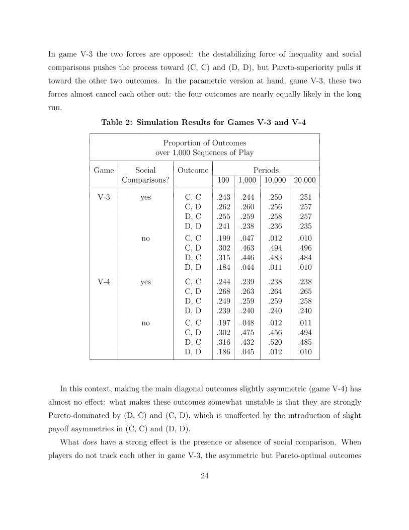
In game V-3 the two forces are opposed: the destabilizing force of inequality and social

comparisons pushes the process toward (C, C) and (D, D), but Pareto-superiority pulls it

toward the other two outcomes. In the parametric version at hand, game V-3, these two

forces almost cancel each other out: the four outcomes are nearly equally likely in the long

run.

Table 2: Simulation Results for Games V-3 and V-4

Proportion of Outcomesover 1,000 Sequences of Play

Game Social Outcome PeriodsComparisons? 100 1,000 10,000 20,000

V-3 yes C, C .243 .244 .250 .251C, D .262 .260 .256 .257D, C .255 .259 .258 .257D, D .241 .238 .236 .235

no C, C .199 .047 .012 .010C, D .302 .463 .494 .496D, C .315 .446 .483 .484D, D .184 .044 .011 .010

V-4 yes C, C .244 .239 .238 .238C, D .268 .263 .264 .265D, C .249 .259 .259 .258D, D .239 .240 .240 .240

no C, C .197 .048 .012 .011C, D .302 .475 .456 .494D, C .316 .432 .520 .485D, D .186 .045 .012 .010

In this context, making the main diagonal outcomes slightly asymmetric (game V-4) has

almost no effect: what makes these outcomes somewhat unstable is that they are strongly

Pareto-dominated by (D, C) and (C, D), which is unaffected by the introduction of slight

payoff asymmetries in (C, C) and (D, D).

What does have a strong effect is the presence or absence of social comparison. When

players do not track each other in game V-3, the asymmetric but Pareto-optimal outcomes

24

now take the lion’s share of the limiting distribution. This shows that it was indeed their

inequality that prevented them from being more stable than the symmetrically bad outcomes

of (C, C) and (D, D) in V-3, with its strongly connected network of social comparisons.

Isolating the Effects of Inequality

As we have seen, the preceding simulations were somewhat complicated to analyze because of

the intertwined effects of inequality and Pareto-dominance. In this last subsection we focus

exclusively on inequality by examining constant-sum games. In such games all outcomes are

necessarily Pareto-optimal. Hence, we can now study the effects of variations in inequality

in splendid isolation.

Consider, for example, the constant-sum game depicted in Figure 8. Whereas there is

enormous inequality in two outcomes, (C, D) and (D, C), payoffs are nearly equal in the

other two outcomes. If Theorem 1 is robust then in the long run (C, C) and (D, D) should

occur more frequently than do the off-diagonal outcomes.

Figure 8: Game V-5 (Constant Sum)

C D

C .01, −.01 −100, 100

D −100, 100 10, −10

However, a simulation of the game V-5 reveals that the outcomes are essentially equally

likely in the long-run (Table 3).16 This would be unsurprising if social comparisons were

disabled but as the table indicates, this occurs when social comparisons are enabled. Indeed,

the output displayed in Table 3 is based on a strong degree of social comparison: when

adjusting aspirations each player puts as much weight on his partner’s payoff as his own.

Despite this, big variations in inequality seem to have no effect: outcomes with nearly equal

payoffs are no more likely in the long-run than those with huge inequalities.

16The final two columns of this figure appear identical. This is not a mistake; the proportions after 10,000periods were virtually identical.

25

Table 3: Simulation Results for Game V-5

Proportion of Outcomesover 1,000 Sequences of Play

Game Social Outcome PeriodsComparisons? 100 1,000 10,000 20,000

V-5 yes C, C .248 .249 .250 .250(magnitude C, D .235 .248 .250 .250insensitive) D, C .268 .252 .250 .250

D, D .250 .250 .250 .250

no C, C .252 .250 .250 .250C, D .246 .249 .250 .250D, C .253 .251 .251 .251D, D .250 .249 .249 .249

V-5 yes C, C .429 .513 .524 .524(magnitude C, D .131 .116 .114 .114sensitive) D, C .315 .282 .276 .276

D, D .124 .089 .086 .086

no C, C .253 .250 .251 .251C, D .248 .249 .249 .249D, C .252 .251 .251 .251D, D .247 .249 .249 .249

26

This anomaly is not confined to a computational model; it reappears in an analytical one.

When players put equal weights on each other’s payoffs and the game is zero-sum, it is easy

to see that both aspirations must converge to zero. This enables us to study the process’s

long-run patterns analytically, if the propensity-adjustment rule is sufficiently simple. For

example, in the bang-bang Bush-Mosteller rule, where propensities adjust completely to zero

or one, the only non-transient propensities are zero and one. Because the long run depends

only on non-transient states, we can analyze this case by examining a reduced form in which

the only propensity-values are zero and one. Further, because we know that the only non-

transient aspiration level is the game’s constant sum, the probability transition matrix that

yields the (unique) invariant distribution for the non-transient states can be represented as

shown in Figure 9, where s denotes the probability that the agent switches to a new action

(i.e., puts a propensity of one on a new action).

Figure 9: Transition Matrix for Non-Transient States in Constant Sum Gamewith Bang-Bang Bush-Mosteller Rule

C, C C, D D, C D, D

C, C 1− s s 0 0

C, D 0 1− s 0 s

D, C s 0 1− s 0

D, D 0 0 s 1− s

This matrix immediately implies that in the unique limiting distribution all outcomes

are equally likely. The simulation got it right.

Why does intuition fail here? Why are the nearly-equal outcomes not much more likely

in the long run than the grossly unequal ones? We believe that this is an artifact of a discon-

tinuity in the propensity-adjustment rule. In the standard Bush-Mosteller rule that drives

these simulations, propensity-change responds only to the sign of feedback; it is insensitive

to magnitudes, e.g., how big is negative feedback. This is why the transition probabilities in

Figure 9 are the same. Our axioms of propensity-adjustment, A1 and A2, do allow for this

magnitude-insensitivity; they do not, however, require it. Accordingly, although Theorem 1

27

and the other analytical results hold for magnitude-insensitive rules such as Bush-Mosteller,

they also hold for rules that respond continuously to feedback. Agents using a magnitude-

sensitive rule would, for example, react more strongly to a big disappointment—payoffs

far below aspirations—than to a small one. And we conjecture that the anomaly would

disappear if the simulation were based on such a rule.

We can test the above reasoning by making propensity-adjustment continuous in the

difference between aspirations and payoffs. Here we assume this in a simple way, by en-

dogenizing the inertia parameter that governs propensity-adjustment. Thus, a player is

inertial—does not change action-propensities—with probability 1 − ψ, which decreases in

the difference between aspirations and payoffs. Assumption A4 expresses the idea formally.

A4 (magnitude-sensitive adjustment): For every agent i the probability of adjustment,

ψ(|ai,t − πi,t|), is a strictly increasing and continuous function, with ψ(0) = 0.

It suffices to make the probability of inertia depend continuously on the magnitude of the

discrepancy between aspirations and payoffs; the rest of the propensity-adjustment mech-

anism can have discontinuities, as does, e.g., the bang-bang Bush-Mosteller. Because this

adaptive rule is so tractable we continue to use it here. Now, however, it is activated with

probability ψ and inactive with the complementary probability.17

If we re-run game V-5 with a magnitude-sensitive propensity-adjustment rule, we see that

here intuition is confirmed: the most nearly-equal outcome is indeed much more likely in the

long-run than highly unequal ones (bottom half of Table 3). As conjectured, the surprising

result for the magnitude-insensitive case shown in the top half of Table 3, which seemed to

indicate that Theorem 1 is not robust, was an artifact of a discontinuity in the simulation’s

propensity-adjustment rule.

The logic underlying this conclusion does not depend on the particular parameter values

used in the magnitude-sensitive simulation. It generalizes to a large class of constant-sum

2× 2 games, as we now show.18

17Because the action of an agent using the bang-bang Bush-Mosteller can be associated with a positivesurprise (i.e., πi,t > ai,t) only if agent i’s propensity to try the action in question already equals the maximumfeasible propensity of 1.0, only the magnitude of disappointments (πi,t < ai,t) matters here.

18This paper’s substantive focus is on collective action problems, which cannot arise in constant-sum gamessince they lack Pareto-suboptimal outcomes—a defining property of collective action problems. Hence thissubsection’s focus on constant sum games is purely methodological: such games allow us to study the effect

28

In what follows, b denotes the sum of the players’ payoffs in a constant-sum game and

p̃(o) is the limiting probability of outcome o.

Remark 1: Consider any constant-sum 2×2 game in which π1(o) 6= π2(o) for all outcomes

o. If ai,t+1 = λiai,t + (1 − λi)πi,t+πj,t

2for i = 1, 2, propensities adjust by a bang-bang

Bush-Mosteller that satisfies A4, and neither player has a strategy that yields more than b2

independently of the other player’s strategy then the following properties hold.

(i) The process is ergodic and the limiting distribution is over four states. The action-

propensities of these four states are defined by the four possible combinations of zero-

one propensities and hence can be described by the four action-pairs: (C,C), (C,D),

(D,C), and (D,D).

(ii) p̃(or) > p̃(os) if and only if |π1(or)− π2(or)| < |π1(os)− π2(os)|.

(iii) ∂p̃(or)∂|π1(or)−π2(or)| < 0.

Part (ii) implies that the more-equal outcomes are more likely in the long-run than are

less-equal ones. Part (iii), a comparative static, says that if an outcome becomes more equal

then it happens more often in the limit.

Remark 1 is confined to 2×2 games. Our last result examines the issue of robustness in a

more general setting. Proposition 2 uses the following notion of a ‘small’ degree of inequality.

We will say that outcome o is in an ε-neighborhood of complete equality if there exists an

ε > 0 such that | bn− πi(o)| ≤ ε for i = 1, . . . , n.

Because we are now examining n-person games, we cannot state simple conditions that

suffice to ensure ergodicity as we could for 2× 2 games. Fortunately, however, this does not

matter, because the next result establishes that the effect of near-equality is close to that of

complete equality for any invariant distribution that the process might reach. (And part (i)

of the proposition shows that it must reach some invariant distribution.)

Proposition 2: Consider any constant-sum game with n > 1 players, where every player

has finitely many actions and in every outcome o there are players i and j such that πi(o) 6=πj(o). If ai,t+1 = λiai,t + (1− λi)

∑nj=1 πj,t

nfor i = 1, . . . , n and action-propensities adjust by a

bang-bang Bush-Mosteller that satisfies A4 then the following hold.

of inequality without the possibly confounding effects of Pareto-inefficiency.

29

(i) The process converges to an invariant distribution.

(ii) If the process has converged to an invariant distribution with exactly one nontransient

outcome, o∗, that is in an ε-neighborhood of complete equality then p̃(o∗) is close to 1

for ε ‘small’.

Proposition 2 shows that when the issue is exclusively how the pie is cut—its size be-

ing constant—and players make social comparisons then the degree of inequality matters,

provided that propensity-adjustment is continuous. This indicates that Theorem 1 and the

other analytical results are robust in a restricted but still important sense: when people

are more likely to respond to big disappointments than to small ones, complete equality is

inessential.

VI. Conclusion

Public outrage based on a experience of relative deprivation has often been suggested as

an explanation for political protest. Yet, in other cases highly unequal societies are stable

without widespread protests. In this paper we propose an explanation for these disparate

findings using a framework that combines adaptive processes based on social comparisons

with strategic interactions analyzed by non-cooperative game theory. Our framework pro-

vides a rich set of results. The first set of findings pertains to general n-person contexts.

We showed that as long as people track the payoffs of some other players, the set of stable

outcomes is tightly restricted: under very general assumptions people must receive the same

payoff in an outcome supported by a self-reinforcing equilibrium. Loosely speaking, social

comparison generates uniformity in payoffs among strongly connected players. Inequality

is not tolerated. If communities are partially decomposable, however, pay-off inequalities

shaped by the reference group structure can endure. What matters at a deeper level is

whether people with low payoffs compare themselves to those with higher ones. If agents

‘look up’ then inequality is unstable. Computational simulations establish the robustness of

the basic intuitions of these analytical results.

The second set of findings showed that similar effects occur in collective action situations.

If agents do not look up, then stable hierarchies of inequality can exist. Actions within a

group are homogenous, but across status groups actions are heterogenous, with higher status

30

groups acting less cooperatively than lower status groups. Thus, we can show the existence

of durable hierarchies of inequality where some groups contribute while others free-ride on

the contributions of the contributing groups. This shows how a socio-psychological property

(“who is in my reference group?”) generates socio-political inequality. Intuitively, the source

of unequal hierarchies is a failure of imagination: one does not compare one’s own payoff

to those of people in other strata. In turn, a shift in social reference groups, either due to

social changes or better access to media, may upset established hierarchies, as individuals

now compare themselves to others that are relatively better off, thus triggering a sense of

dissatisfaction that may ultimately lead to political unrest and other forms of collective

action.

Our results also shed some light on the impact of social media on social movements and

revolts as recently witnessed in the “Arab Spring” (Eltantawy and Wiest, 2011). Many com-

mentators have focused on how social media have allowed political activists and opposition

groups to organize more quickly. Our results suggest that new media may also change so-

cial reference groups. Once people of lower socio-economic status compare their lot to that

enjoyed by the better-off, unequal payoffs can no longer be sustained.

31

Appendix

Proof of Theorem 1

Sufficiency. Consider an outcome o in which everyone gets the same payoff, π(o). The

candidate pure SRE (i.e., one in which everyone plays pure strategies) is one in which player

i plays αi(o) with probability one and in which ai,t = π(o) for all i.

Because aspirations equal π(o), everyone is satisfied in t, whence by (A1) player i con-

tinues to play αi(o) with probability one, for all i.

Further, because everyone is getting the same payoff, by A3 everyone is getting a weighted

average of π(o) for any realized Λ. Hence ai,t+1 = ai,t.

Thus, the propensity and aspiration vectors of period t are reproduced in t+ 1. QED.

Necessity. The proof is by contradiction. Suppose that an outcome o∗ is supported by a

pure SRE (i.e., one in which everyone plays pure strategies) but in o∗ there are at least two

people who get different payoffs. That is, there exists an SRE such that

for all i and t : pi,t(αi(o∗)) = 1 and ai,t ∈ Ai,

where Ai has the properties stipulated by Definition 1, and there exist some distinct i and

j such that πi(o∗) 6= πj(o

∗).

Because there are at least two players, i and j, who get different payoffs in o∗, we can

partition N into two nonempty subsets, A and B, such that everyone in A gets the same

payoff and everyone in B gets a higher one. (Note that the payoff to players in A is not

necessarily the minimal payoff in o∗; it is simply less than the payoffs of any of the B players.)

Now consider some i ∈ A, and suppose that we are trying to stabilize the vector of pure

propensities that generates o∗ and the associated sets of aspirations at some date t. (Recall

that because |L| ≥ 1, social comparisons may continually change, whence so may aspirations,

even in an SRE.)

Because the group is probabilistically strongly connected there must be at least one player

in A, say i, at least one player in B, say j, and some Λq ∈ L such that Λqi,j > 0.

We consider three cases.

Case 1: ai,t > πi(o∗).

32

Because A2 requires that the action-propensity change whereas the definition of an SRE

requires that it remain fixed, in this case we are done immediately.

Case 2: ai,t = πi(o∗).

Because player i tracks j ∈ B in at least one Λ, i.e., in Λq, and because ρq > 0, Pr(i tracks

nobody in B in t) < 1. Hence, ai,t is not absorbing; further, in every period the process

can transition to Case 1 with a probability that is bounded away from zero uniformly in t.

Therefore the condition that defines case 2 cannot be part of an SRE.

Case 3: ai,t < πi(o∗).

Because here ai,t < πi(o∗) and because ai,t+1 is a weighted average of ai,t, πi(o

∗), and

other payoffs (associated with o∗) which, because i ∈ A, must all weakly exceed πi(o∗), it

follows immediately that ai,t+1 > ai,t. Hence, no set of aspirations (a, a), where a < πi(o∗),

is absorbing. Further, because the set of social influence matrices is fixed and each one

is realized with a probability that is bounded away from zero uniformly in t, the second

Borel-Cantelli lemma implies that the probability that ai,t stays below πi(o∗) goes to zero as

t→∞. Further, since i must be tracking players whose payoffs strictly exceed his, eventually

the process must transition to case 1, whereupon the argument pertaining to that case is

activated. QED.

In the proof of Proposition 1 and thereafter we follow the convention of using ‘with posi-

tive probability’ (abbreviated by ‘wpp’) as a shorter way of saying “with strictly positive

probability.”

Proof of Proposition 1

The proof is by contradiction. Suppose outcome o, which yields unequal payoffs, is supported

by an SRE yet there is some player, say i, who gets the minimum payoff and who wpp tracks

j, whose payoff exceeds i’s. Then for any social influence matrix for which Λi,j(o) > 0,

ai,t > πi. But then by A2, the axiom of negative feedback, i’s propensity to play αi(o) must

decrease. Hence the assumption that o is supported by an SRE must be false. QED.

33

Proof of Theorem 2

(i) We check to see whether outcome o′, in which Ar-payoffs are heterogeneous, can be

supported by an SRE. Since Ar is sealed off from the other groups, regarding aspirational

dynamics we can treat it as a free-standing set of players. Hence, Theorem 1 can be applied.

So the answer is negative: outcome o′ cannot be supported by an SRE.

(ii) Select an arbitrary group, Ar. We check to see whether a certain outcome o, which

gives everyone in Ar the same payoff, πAr(o), can be supported by an SRE. (Given that Ar

was selected arbitrarily, if this works for Ar then it will work generally.) Suppose in some

period o occurs. We construct vectors of aspirations and propensities that will self-replicate,

in the sense of Definition 1. First, let ai,t ≤ πAr(o) for all i ∈ Ar. Second, let Pr(αi(o)) = 1.

Since i tracks only other people in Ar and since in t everyone in Ar gets the same payoff

from o, ai,t+1 = λiai,t + (1 − λi)πAr(o). Hence ai,t+1 ≤ πAr(o), so the players continue to

be satisfied by o. Moreover, by simple algebra, all their aspirations continue to be less than

or equal to π(o). By induction these properties continue to hold indefinitely, satisfying the

definition of a self-replicating equilibrium. QED.

Proof of Theorem 3

Sufficiency. If everyone gets the same payoff then any convex combination of payoffs (i.e.,

any combination of Λi,j’s) is also the same; call this π. Consider one of these outcomes; call

it o. Consider any start in which Pr(αi(o)) = 1 and ai,0 ≤ π for all i. Then everyone is

satisfied in o so by A1 all propensities continue, in t = 2, to equal one on the appropriate

action. Further, by A3 all aspirations continue to be less than or equal to π in t = 2. By

induction these properties continue to hold indefinitely, whence o is an SRE. QED.

Necessity. Consider an outcome o (without loss of generality in the public good game) in

which payoffs are heterogeneous. Hence there must be at least two players, say i and j, such

that πi(o) < πj(o). Because aspirations are formed by looking up, i tracks only players who

get more than πi(o). And because λi + Λi,i < 1, i must track someone wpp. Hence wpp ai

is a convex combination of i’s payoff and something greater than that, whence ai > πi(o).

In such an event i is dissatisfied, and by A2 reduces her propensity to play αi(o). So o is

unstable. QED.

34

Proof of Theorem 4

Consider an arbitrary player i. At any date t, either i tracks someone else or she does not.

If she does not then ai,t = πi,t. If she does, then she tracks someone who gets a payoff that

is equal to or less than πi,t. In this case, ai,t ≤ πi,t. In either case she is satisfied with the

outcome, o; hence by A1 she will not reduce the propensity to play αi(o). Therefore the

state in which i plays αi(o) with probability one and in which ai = πi(o), for i = 1, . . . , n, is

stable. QED.

Proof of Corollary 1

Sufficiency Consider an outcome o in which the ambitious players get the maximal payoff,

π(o). Because nobody’s payoff exceeds theirs, they are satisfied no matter whom they track.

And since unambitious players look down or sideways, the proof of Theorem 4 holds for this

subset. Hence everyone is satisfied in o, so by the usual construction o is an SRE. QED.

Necessity Consider an outcome o in which some ambitious player, say i, is not getting the

maximal payoff. Since λi + Λi,i < 1, wpp i tracks someone else. And since i only looks up,

anyone who is tracked by i, say j, must satisfy πi(o) < πj(o). Hence ai(o) > πi(o). Thus i is

dissatisfied, which destabilizes o. QED.

Proof of Corollary 2

Since conflictual games are symmetric, if everyone takes the same action (in say the public

goods game) then they all get the same payoff. Then Theorem 3 can be applied. QED.

Proof of Corollary 3

Because the game is conflictual, hence symmetric, all players have the same action set.

Therefore, mi = m for all i. Further, it is given that m ≥ k, where k is the number of

groups. (To avoid triviality we assume that k > 1.) Thus, without loss of generality we can

label the groups and the actions so that in outcome o players in group j use action αj, where

j = 1, . . . , k. Then Theorem 4, which holds for arbitrary outcomes, can be applied. QED.

35

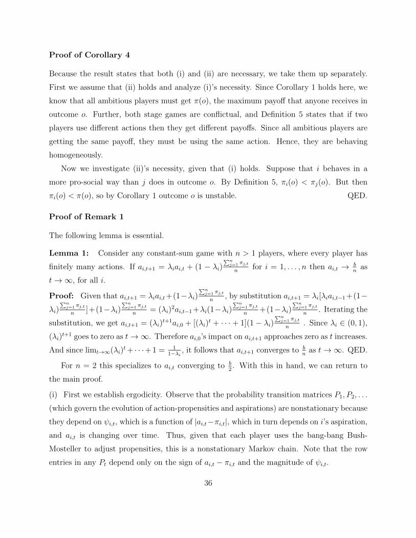
Proof of Corollary 4

Because the result states that both (i) and (ii) are necessary, we take them up separately.

First we assume that (ii) holds and analyze (i)’s necessity. Since Corollary 1 holds here, we

know that all ambitious players must get π(o), the maximum payoff that anyone receives in

outcome o. Further, both stage games are conflictual, and Definition 5 states that if two

players use different actions then they get different payoffs. Since all ambitious players are

getting the same payoff, they must be using the same action. Hence, they are behaving

homogeneously.

Now we investigate (ii)’s necessity, given that (i) holds. Suppose that i behaves in a

more pro-social way than j does in outcome o. By Definition 5, πi(o) < πj(o). But then

πi(o) < π(o), so by Corollary 1 outcome o is unstable. QED.

Proof of Remark 1

The following lemma is essential.

Lemma 1: Consider any constant-sum game with n > 1 players, where every player has

finitely many actions. If ai,t+1 = λiai,t + (1 − λi)∑n

j=1 πj,t

nfor i = 1, . . . , n then ai,t → b

nas

t→∞, for all i.

Proof: Given that ai,t+1 = λiai,t+(1−λi)∑n

j=1 πj,t

n, by substitution ai,t+1 = λi[λiai,t−1+(1−

λi)∑n

j=1 πj,t

n]+(1−λi)

∑nj=1 πj,t

n= (λi)

2ai,t−1+λi(1−λi)∑n

j=1 πj,t

n+(1−λi)

∑nj=1 πj,t

n. Iterating the

substitution, we get ai,t+1 = (λi)t+1ai,0 + [(λi)

t + · · · + 1](1− λi)∑n

j=1 πj,t

n. Since λi ∈ (0, 1),

(λi)t+1 goes to zero as t→∞. Therefore ai,0’s impact on ai,t+1 approaches zero as t increases.

And since limt→∞(λi)t + · · ·+ 1 = 1

1−λi , it follows that ai,t+1 converges to bn

as t→∞. QED.

For n = 2 this specializes to ai,t converging to b2. With this in hand, we can return to

the main proof.

(i) First we establish ergodicity. Observe that the probability transition matrices P1, P2, . . .

(which govern the evolution of action-propensities and aspirations) are nonstationary because

they depend on ψi,t, which is a function of |ai,t−πi,t|, which in turn depends on i’s aspiration,

and ai,t is changing over time. Thus, given that each player uses the bang-bang Bush-

Mosteller to adjust propensities, this is a nonstationary Markov chain. Note that the row

entries in any Pt depend only on the sign of ai,t − πi,t and the magnitude of ψi,t.

36

Because Lemma 1 implies that ai,t is converging to b2

as t → ∞, it follows that ψi,t →ψi(| b2 − πi,t|) as t→∞ for i = 1, 2. Hence the sequence of probability transition matrices is

itself converging to a stationary P∞. Therefore, by Lemma 2 in Anily and Federgruen (1987,

p. 869), if a nonstationary Markov chain satisfies Pt → P∞ and P∞ is ergodic then the

nonstationary Markov chain is itself ergodic: it has a unique invariant distribution over its

state space and it must converge to that vector of probabilities from any initial distribution.

Thus far, however, we know only that the sequence of Pt’s converges to some stationary

P∞; we do not yet know whether P∞ is ergodic. Hence we must show that, given the

assumptions of Remark 1, P∞ does in fact represent an ergodic process. To do this, note

first that because the game is constant sum, πi,t >b2

if and only if πj,t <b2. Thus, since

πi(o) 6= πj(o) in all four outcomes of this 2×2 game, exactly one player is dissatisfied in every

outcome, given aspirations of b2. Therefore, the dynamics of the process can be represented

by the following schematic matrix.

C D

C +, − −, +

→ ↓

D −, + +, −↑ ←

At this point the assumption that neither player has a strategy that guarantees satisfac-

tion for ai,t = b2

is useful. It is easy to see that this condition implies that each player is

satisfied in exactly two outcomes. (If, e.g., player 1 were satisfied in three outcomes then

she must have a strategy that ensures a satisfactory payoff for her regardless of player 2’s

action.) Given this restriction, it follows that there are only two possibilities. Stated from

the perspective of player 1, they are (1) player 1 is satisfied by (C, C) and (D, D) or (2)

she is satisfied by (C, D) and (D, C). In the other four cases either action C or action D is

unconditionally satisfying for player 1 or an action is unconditionally satisfying for player 2.

In possibility (1), transitions in the schematic matrix move clockwise; in (2), counter-

clockwise. In either case the process can reach any of the four action-combinations from any

of the others. Hence the states of P∞ communicate. Further, since ψ(·) is strictly increasing

37

in the disparity between aspirations and payoffs, it follows that the probability of inertia (a

dissatisfied player not changing his propensities) is strictly positive in every outcome. This

ensures aperiodicity. Hence P∞ is, in fact, ergodic. As we’ve seen, the limiting distribution

is over all four states, which are described as the four action-combinations, i.e., result (ii)(a)

holds. Thus P∞ is as follows. (Without loss of generality this matrix is based on possibility

(1): (C, C) and (D, D) are satisfying for player 1. The logic for the other matrix is identical.)

C, C C, D D, C D, D

C, C 1−ψ(| b2−π2(C,C)|) ψ(| b

2−π2(C,C)|) 0 0

C, D 0 1−ψ(| b2−π1(C,D)|) 0 ψ(| b

2−π1(C,D)|)

D, C ψ(| b2−π1(D,C)|) 0 1−ψ(| b

2−π1(D,C)|) 0

D, D 0 0 ψ(| b2−π2(D,D)|) 1−ψ(| b

2−π2(D,D)|)

Given this matrix, a bit of algebra reveals that p̃(state i)p̃(state j)

equals the inverse of their exit-

probabilities; e.g., p̃(C,C)p̃(C,D)

=ψC,D

ψC,C. Thus, the states’ limiting probabilities are ordered inversely

to their associated dissatisfaction probabilities, which establishes (ii).

Further, because the ratio of state i’s limiting probability against any other state’s lim-

iting probability is decreasing in ψi, it follows that p̃(state i) is decreasing in ψi, which

establishes (iii). QED.

Proof of Proposition 2

(i) The first step in proving that the process must converge to some invariant distribution

is to note that because the stage game is constant sum and aspirations adjust via ai,t+1 =

λiai,t + (1− λi)∑n

j=1 πj,t

n, a straightforward extension of the two-player result of Remark 1 to

this n-player setting yields the fact that ai,t converges to bn

as t→∞, for all i. This in turn

implies that the sequence of probility transition matrices is converging to a stationary P∞.

Since this stationary matrix governs a finite-state Markov chain it must have at least one

invariant distribution. Finally, convergence is ensured because A4 implies that there must

be inertia in propensity-adjustment, which means that the process is aperiodic. QED.

(ii) Either P∞ yields a unique invariant distribution or multiple ones. If there is only

one then the states’ limiting probabilities can be computed via P∞. Because these limiting

38

probabilities are continuous in the matrix’s transition probabilities and because o∗ would be

absorbing if all its payoffs were exactly the same, the result follows. If there are multiple

invariant distributions then each one must be over a closed class of states, so in effect there

are multiple Markov chains that can be analyzed independently: the limiting probabilities for

a given closed class of states can be calculated by the corresponding submatrix of transition

probabilities, and the continuity property holds as before. QED.

39

References

Anily, Shoshana, and Awi Federgruen. 1987. Ergodicity in Parametric Nonstationary

Markov Chains. Operations Research 35(6):867-874.

Bendor, Jonathan, Daniel Diermeier, and Michael Ting. 2003. A Behavioral Model of

Turnout. American Political Science Review 97(2):261-280.

Bendor, Jonathan, Daniel Diermeier, and Michael Ting. 2007a. Comment: Adaptive

Models in Sociology and the Problem of Empirical Content. American Journal of

Sociology 112(5):1534-1545.

Bendor, Jonathan, Daniel Diermeier, and Michael Ting. 2007b. Aspirations, Reference

Groups, and Collective Action. Paper presented at the the 2007 Annual Meeting of

the American Political Science Association.

Bendor, Jonathan, Daniel Diermeier, David Siegel, and Michael Ting. 2011. A Behavioral

Theory of Elections. Princeton, NJ: Princeton University Press.

Bendor, Jonathan, and Dilip Mookherjee. 1990. Norms, Third-Party Sanctions, and Co-

operation. Journal of Law, Economics, and Organization 6(1):33-63.

Blanton, Hart, Bram P. Buunk, Frederick X. Gibbons, and Hans Kuyper. 1999. When

Better-Than-Others Compare Upward: Choice of Comparison and Comparative Eval-

uation as Independent Predictors of Academic Performance. Journal of Personality &

Social Psychology 76(3):420-430.

Buunk, Bram, Rebecca Collins, Shelley Taylor, Nico Van Yperen, and Gayle Dakof. 1990.

The Affective Consequences of Social Comparison: Either Direction Has Its Ups and

Downs. Journal of Personality & Social Psychology 59(6):1238-1249.

Bush, Robert, and Frederick Mosteller. 1955. Stochastic Models for Learning. New York:

Wiley.

Caporale, Guglielmo M., Yannis Georgellis, Nicholas Tsitsianis, and Ya Ping Yin. 2009.

Income and happiness across Europe: Do reference values matter? Journal of Economic

Psychology 30(1):42-51.

40

Clark, Andrew E., Paul Frijters, and Michael A. Shields. 2008. Relative Income, Happiness,

and Utility: An Explanation for the Easterlin Paradox and Other Puzzles. Journal of

Economic Literature 46(1):95-144.

Collins, Rebecca. 1996. For Better or Worse: the Impact of Upward Social Comparison on

Social-Evaluations. Psychological Bulletin 119(1):51-69.

Cross, John. 1973. A Stochastic Learning Model of Economic Behavior. Quarterly Journal

of Economics 87(2):239-266.

Cui, Zhiwei, Jian Zhai, and Xuan Liu. 2009. The Efficiency of Observability and Mutual

Linkage. The B.E. Journal of Theoretical Economics 9(1) (Contributions), Article 23.

Davies, James C. 1962. Toward a Theory of Revolution. American Sociological Review

27(1):5-19.

Eltantawy, Nahed, and Julie B. Wiest. 2011. The Arab Spring — Social Media in the Egyp-

tian Revolution: Reconsidering Resource Mobilization Theory. International Journal

of Communication 5:1207-1224.

Festinger, Leon. 1954. A Theory of Social Comparison Processes. Human Relations 1:117-

140.

Fliessbach, K., B. Weber, P. Trautner, T. Dohmen, U. Sunde, C. E. Elger, and A. Falk.

2007. Social Comparison Affects Reward-Related Brain Activity in the Human Ventral

Striatum. Science 318:1305-1380.

Gerrard, Meg, Frederick X. Gibbons, David J. Lane, and Michelle L. Stock. 2005. Smoking

cessation: Social comparison level predicts success for adult smokers. Health Psychology

24(6):623-629.

Gurney, Joan N., and Kathleen J. Tierney. 1982. Relative Deprivation and Social Move-

ments: A Critical Look at Twenty Years of Theory and Research. The Sociological

Quarterly 23(1):33-47.

Gurr, Ted Robert. 1970. Why Men Rebel. Princeton, NJ: Princeton University Press.

41

Helgeson, Vicki S., and Shelley E. Taylor. 1993. Social Comparisons and Adjustment

Among Cardiac Patients. Journal of Applied Social Psychology 23(15):1171-1195.

Jackson, Matthew O. 2008. Social and Economic Networks. Princeton, NJ: Princeton

University Press.

Kandori, Michiko. 1992. Social Norms and Community Enforcement. Review of Economic

Studies 59(1):63-80.

Karlsson, Niklas, Peter Dellgran, Birgitta Klingander, and Tommy Garling. 2004. House-

hold consumption: Influences of aspiration level, social comparison, and money man-

agement. Journal of Economic Psychology 25(6):753-769.

Kayser, Mark A., and Michael Peress. 2012. Benchmarking across Borders: Electoral

Accountability and the Necessity of Comparison. American Political Science Review

106(3):661-684.

Lazer, David, Brian Rubineau, Carol Chetkovich, Nancy Katz, and Michael Neblo. 2010.

The Coevolution of Networks and Political Attitudes. Political Communication 27(3):248-

274.

Luttmer, Erzo F. P. 2005. Neighbors as Negatives: Relative Earnings and Well-Being.

Quarterly Journal of Economics 120(3):963-1002.

Macy, Michael, and Andreas Flache. 2002. Learning Dynamics in Social Dilemmas. Pro-

ceedings of the National Academy of Sciences 99:7229-7236.

Olson, Mancur. 1971 [1965]. The Logic of Collective Action: Public Goods and the Theory

of Groups, Revised Edition. Cambridge, MA: Harvard University Press.

Ostrom, Elinor. 1990. Governing the Commons: The Evolution of Institutions for Collec-

tive Action. New York: Cambridge University Press.

Runciman, Walter G. 1966. Relative Deprivation and Social Justice: A Study of Atti-

tudes to Social Inequality in Twentieth-Century England. Berkeley, CA: University of

California Press.

Sherif, M. 1936. The Psychology of Social Norms. Oxford, UK: Harper.

42

Stiglitz, Joseph. 2011. Of the 1%, by the 1%, for the 1%. Vanity Fair, May.

Suls, Jerry, Christine A. Marco, and Sheldon Tobin. 1991. The Role of Temporal Com-

parison, Social Comparison, and Direct Appraisal in the Elderly’s Self-Evaluations of

Health. Journal of Applied Social Psychology 21(14):1125-1144.

Taylor, Shelley, and Marci Lobel. 1989. Social Comparison Activity under Threat: Down-

ward Evaluation and Upward Contacts. Psychological Review 96(4):569-575.

Tilly, Charles. 1992. Coercion, Capital, and European States. Cambridge, MA: Blackwell.

Van der Zee, Karen, Bram Buunk, and Bram Sanderman. 1998. Neuroticism and Reactions

to Social Comparison Information Among Cancer Patients. Journal of Personality

66(2):175-194.

Veenhoven, Ruut. 1991. Is Happiness Relative? Social Indicators Research 24(1):1-34.

Wills, Thomas. 1981. Downward Comparison Principles in Social Psychology. Psycholog-

ical Bulletin 90(2):245-271.

43