Inequality and Economic Growth in Brazil - UZH and Economic Growth in Brazil ... based Kuznets'...
41
Transcript of Inequality and Economic Growth in Brazil - UZH and Economic Growth in Brazil ... based Kuznets'...
Inequality and Economic Growth inBrazil
Bachelor's Thesis
supervised by the
Department of Economics at the University of Zurich
Prof. Dr. Fabrizio Zilibotti
to obtain the degree of
Bachelor of Arts in Economics
Author: Yves KellerCourse of Studies: Economics
1
Abstract
This bachelor thesis gives an overview over Brazil's inequality
and provides the economic theory and latest �ndings about the re-
lationship between inequality and economic growth. In an empirical
part the paper shows with newer data that a signi�cant inequality-
based Kuznets' curve exists for the case of Brazil and that the level
of GDP alone can explain most of the variation in inequality. In a
single-country growth regression the paper �nds evidence that edu-
cation was the main contributor to economic growth in the last half
century and that the Gini coe�cient is insigni�cant when it comes
to its in�uence on growth in Brazil.
2
Contents
1 Introduction 5
2 Inequality in Brazil 8
2.1 Inequality measures . . . . . . . . . . . . . . . . . . . . . . . . . 8
2.2 Facts and �gures about Brazil's inequality . . . . . . . . . . . . . 10
2.3 Why is Brazil so unequal . . . . . . . . . . . . . . . . . . . . . . 12
3 Theoretical Channels on how growth can be a�ected 16
3.1 Credit-market imperfections . . . . . . . . . . . . . . . . . . . . . 17
3.2 Redistribution programs . . . . . . . . . . . . . . . . . . . . . . . 17
3.3 Sociopolitical unrest . . . . . . . . . . . . . . . . . . . . . . . . . 18
3.4 Saving rates . . . . . . . . . . . . . . . . . . . . . . . . . . . . . . 18
3.5 Further channels . . . . . . . . . . . . . . . . . . . . . . . . . . . 18
3.6 Net e�ect . . . . . . . . . . . . . . . . . . . . . . . . . . . . . . . 19
3.7 Situation in Brazil . . . . . . . . . . . . . . . . . . . . . . . . . . 19
4 Empirical �ndings on the e�ect on growth 22
4.1 Evidence of Kuznets curve . . . . . . . . . . . . . . . . . . . . . . 23
4.2 Cross-country regressions . . . . . . . . . . . . . . . . . . . . . . 24
4.3 Implications and problems . . . . . . . . . . . . . . . . . . . . . . 25
5 Regressions 26
5.1 Data set . . . . . . . . . . . . . . . . . . . . . . . . . . . . . . . . 27
5.2 Kuznets' curve in Brazil . . . . . . . . . . . . . . . . . . . . . . . 28
5.2.1 Model . . . . . . . . . . . . . . . . . . . . . . . . . . . . . 28
5.2.2 Results . . . . . . . . . . . . . . . . . . . . . . . . . . . . 29
5.3 Determinants of Income Inequality . . . . . . . . . . . . . . . . . 30
5.3.1 Model . . . . . . . . . . . . . . . . . . . . . . . . . . . . . 30
5.3.2 Results . . . . . . . . . . . . . . . . . . . . . . . . . . . . 31
5.4 E�ect on Growth . . . . . . . . . . . . . . . . . . . . . . . . . . . 32
5.4.1 Model . . . . . . . . . . . . . . . . . . . . . . . . . . . . . 32
5.4.2 Results . . . . . . . . . . . . . . . . . . . . . . . . . . . . 32
5.5 Discussion . . . . . . . . . . . . . . . . . . . . . . . . . . . . . . . 34
6 Conclusion 36
3
List of Figures
1 PPP GDP per capita in US Dollar for Brazil 1981-2009. . . . . . 5
2 Real GDP growth rate for Brazil 1999-2010 . . . . . . . . . . . . 6
3 GDP per capita vs. Inequality . . . . . . . . . . . . . . . . . . . 7
4 Gini-coe�cient on income inequality in Brazil 1981-2009. . . . . 11
5 Income distribution in Brazil 2009 . . . . . . . . . . . . . . . . . 12
List of Tables
1 Income shares in Brazil 2009 . . . . . . . . . . . . . . . . . . . . 11
2 Education levels in Brazil 2010 . . . . . . . . . . . . . . . . . . . 13
3 Data sources - Overview . . . . . . . . . . . . . . . . . . . . . . . 28
4 Data information . . . . . . . . . . . . . . . . . . . . . . . . . . . 28
5 Results from Kuznets curve regression . . . . . . . . . . . . . . . 29
6 Results: Determinants of Income Inequality . . . . . . . . . . . . 31
7 Results: E�ect on Growth . . . . . . . . . . . . . . . . . . . . . . 34
4
1 Introduction
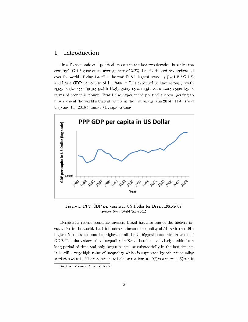
Brazil's economic and political success in the last two decades, in which the
country's GDP grew at an average rate of 3.2%, has fascinated researchers all
over the world. Today, Brazil is the world's 8th largest economy (by PPP GDP)
and has a GDP per capita of $ 11`600. 1 It is expected to have strong growth
rates in the near future and is likely going to overtake even more countries in
terms of economic power. Brazil also experienced political success, getting to
host some of the world's biggest events in the future, e.g. the 2014 FIFA World
Cup and the 2016 Summer Olympic Games.
����
�������������� ������������������
����
������������������ �������
Figure 1: PPP GDP per capita in US Dollar for Brazil 1981-2009.Source: Penn World Table 2012
Despite its recent economic success, Brazil has also one of the highest in-
equalities in the world. Its Gini index on income inequality of 51.9% is the 19th
highest in the world and the highest of all the 20 biggest economies in terms of
GDP. The data shows that inequality in Brazil has been relatively stable for a
long period of time and only began to decline substantially in the last decade.
It is still a very high value of inequality which is supported by other inequality
statistics as well: The income share held by the lowest 10% is a mere 1.1% while12011 est. (Source: CIA Factbook)
5
��
�
�
�
�
�
�
�
���� ���� ���� ���� ���� ���� ���� ���� ��� ��� ���� ����
����������� ��� ��������
����
����������� ��� �
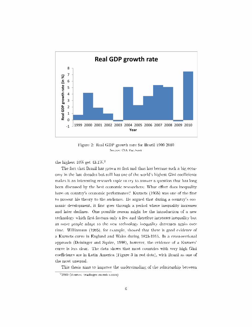
Figure 2: Real GDP growth rate for Brazil 1999-2010Source: CIA Factbook
the highest 10% get 43.1%.2
The fact that Brazil has grown so fast and thus has become such a big econ-
omy in the last decades but still has one of the world's highest Gini coe�cients
makes it an interesting research topic to try to answer a question that has long
been discussed by the best economic researchers: What e�ect does inequality
have on country's economic performance? Kuznets (1955) was one of the �rst
to present his theory to the audience. He argued that during a country's eco-
nomic development, it �rst goes through a period where inequality increases
and later declines. One possible reason might be the introduction of a new
technology which �rst favours only a few and therefore increases inequality but
as more people adapt to the new technology inequality decreases again over
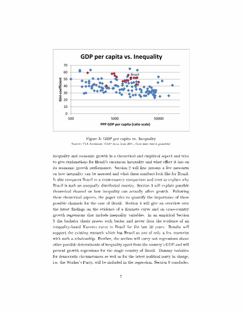
time. Williamson (1985), for example, showed that there is good evidence of
a Kuznets curve in England and Wales during 1823-1915. In a cross-sectional
approach (Deininger and Squire, 1998), however, the evidence of a Kuznets'
curve is less clear. The data shows that most countries with very high Gini
coe�cients are in Latin America (Figure 3 in red dots), with Brazil as one of
the most unequal.
This thesis aims to improve the understanding of the relationship between22009 (Source: tradingeconomics.com)
6
������
�
��
�
�
��
��
�
��
��� ���� �����
���������������
������������������� ������
������������� ����������
Figure 3: GDP per capita vs. InequalitySource: CIA Factbook (GDP data from 2011, Gini data latest possible)
inequality and economic growth in a theoretical and empirical aspect and tries
to give explanations for Brazil's enormous inequality and what e�ect it has on
its economic growth performance. Section 2 will �rst present a few measures
on how inequality can be assessed and what these numbers look like for Brazil.
It also compares Brazil in a cross-country comparison and tries to explain why
Brazil is such an unequally distributed country. Section 3 will explain possible
theoretical channel on how inequality can actually a�ect growth. Following
these theoretical aspects, the paper tries to quantify the importance of these
possible channels for the case of Brazil. Section 4 will give an overview over
the latest �ndings on the evidence of a Kuznets curve and on cross-country
growth regressions that include inequality variables. In an empirical Section
5 the bachelor thesis proves with better and newer data the evidence of an
inequality-based Kuznets curve in Brazil for the last 50 years. Results will
support the existing research which has Brazil as one of only a few countries
with such a relationship. Further, the section will carry out regressions about
other possible determinants of inequality apart from the country's GDP and will
present growth regressions for the single country of Brazil. Dummy variables
for democratic circumstances as well as for the latest political party in charge,
i.e. the Worker's Party, will be included in the regression. Section 6 concludes.
7
2 Inequality in Brazil
As described in the Introduction, Brazil is infamous for its extreme inequality
with a Gini index on income inequality of 51.9%. However, there are more than
one method to describe a country's inequality and some of them will be explained
in the �rst subchapter. In a second part the results for Brazil are presented and
put in a world wide context. In a �nal subchapter, I will summarize the �ndings
in economic literature on why Brazil is so unequal.
2.1 Inequality measures
First and foremost it has to be said that there is no such thing as the
right inequality measurement. The question which method should be chosen is
dependable on what speci�c point the author wants to focus or on how suitable
the method is in explaining the given problem. In addition, most of the time
researchers have to rely on the available data collected by national and regional
governments. Calculating inequality is something not only done by economists
but also by scientists in many other �elds, ranging from social sciences to natural
sciences.
Properties
Despite di�erent methods in calculating inequality, there are four proper-
ties that scientists can agree on (Cowell and Victoria-Feser, 1996): (1) it should
make no di�erence in the calculation which person owns a speci�c income share,
(2) richer countries should not by construction be labelled more unequal (scale
independence), (3) a higher population should have no e�ect on the measure-
ment (population independence) and (4) a transfer from a richer person to a
poorer person while still preserving the order of income ranks should decrease
and not increase inequality.
Gini index
By far the most famous and most used method in measuring inequality is
the Gini index. De�ning the area between the the line of perfect equality and
the Lorenz curve as A and the area under the Lorenz curve as B (see also Figure
5 later in this chapter for the case of Brazil), the Gini index is given by:
Gini = A(A+B)
Gini = A0.5 = 2A = 1− 2B
8
If the Lorenz curve is given by a function y = f(x), the Gini index can be
found like this:
Gini = 1− 2´ 10f(x)dx
In reality, though, the Lorenz curve is almost always unknown and often
only certain points on the curve, i.e. income shares of certain population shares,
are aquired in surveys. This makes the calculation of the area B easier but it
must be said that those results represent only approximations. Barro (2000),
for example, uses that kind of approximation, a Gini index based on income
quintile-shares �rst introduced by Theil (1967). A Gini index can take values
from 0 to 1 with 0 being a total equal and 1 a total unequal society. For further
research and more advanced methods one can have a look at Theil (1969),
Ogwang (2000), Giles (2004) or Deaton (1997) who established a very simple
formula for calculating the Gini index with only the mean of the distribution,
the population and the income shares.
Hoover index
The Hoover index, also called Robin Hood index, is an other measure of
inequality that is used by scientists (Hoover, 1936). It describes how much of
a country's or region's income had to transferred from the rich segment to the
poor one in order to have a community that is totally equal. Graphically, it is
represented by the largest di�erence between the total equality curve and the
Lorenz curve. As with the Gini index, the Hoover index can take values from 0
to 1 with 0 being a total equal community.
Further indexes
The Theil index (Theil, 1967) and the Atkinson index (Atkinson, 1970) are
two more complex indexes which are both based on entropy indexes origing in
information theory. These indexes are preferred when subgroup inequality, i.e.
inequality among income share groups, should also be considered. However,
for most economic research and also for this paper, such indexes are not often
made use of and the Gini index is commonly preferred due to its simplicity and
availability in statistical research.3
3For further study: Atkinson and Bourguignon (2000) and Sen and Foster (1996)
9
Income-share and ratios
An other well used method in describing a community's inequality is to take
a look at income shares. Those shares explain how much a certain share of
population gets from the total income. Usually, one is most interested in the
highest- and lowest-income shares, usually with values that range from 0.1%
to 20% of the population. For comparing those shares' income di�erences, re-
searchers often build ratios to explain by how many times one group is better
o� than an other. Therefore, it's usually higher income groups over lower in-
come groups. Those income shares can also be compared to mean or median
values to get more comparable results. One huge disadvantage compared to the
above stated indexes might be that ratios do not provide absolute measures of
inequality.
After summarizing the most important ways how to calculate inequality, one
important point should not be forgotten and starts before choosing an adequate
method in analysing the inequality. That is the answer of which inequality
should be measured. An economic researcher has to distinguish between income
and wealth inequality; and if he chooses income inequality, does it include capital
gains or not. He also has to decide whether to look at individuals or household
and if he wants to focus on inequality before or after tax. The di�erent methods
for putting a number on inequality explain practically the same thing, but can
sometimes vary a bit in their levels. For high inequalities, the Theil index is
larger than the Hoover index, while for low inequalities, it is the other way round
(Deaton, 1997). In general, most research done on the topic of inequality uses
a second inequality measure to test their results' robustness. Barro (2000) used
the Gini coe�cient in his main regressions and tested his �ndings against the
lowest and the highest income-quintile share to con�rm his original regression
results.
2.2 Facts and �gures about Brazil's inequality
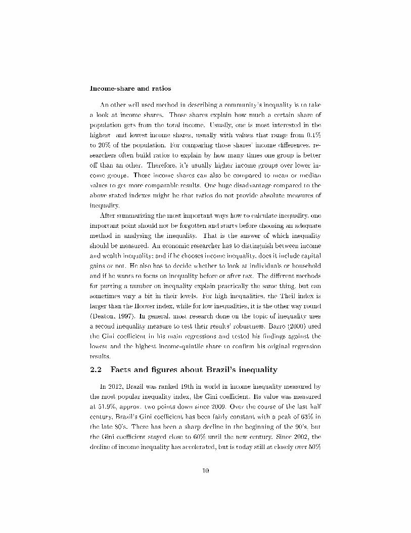
In 2012, Brazil was ranked 19th in world in income inequality measured by
the most popular inequality index, the Gini coe�cient. Its value was measured
at 51.9%, approx. two points down since 2009. Over the course of the last half
century, Brazil's Gini coe�cient has been fairly constant with a peak of 63% in
the late 80's. There has been a sharp decline in the beginning of the 90's, but
the Gini coe�cient stayed close to 60% until the new century. Since 2002, the
decline of income inequality has accelerated, but is today still at closely over 50%
10
��
��
��
��
��
��
��
��
��
������������������
����
���������������
Figure 4: Gini-coe�cient on income inequality in Brazil 1981-2009.Source: Index Mundi 2012
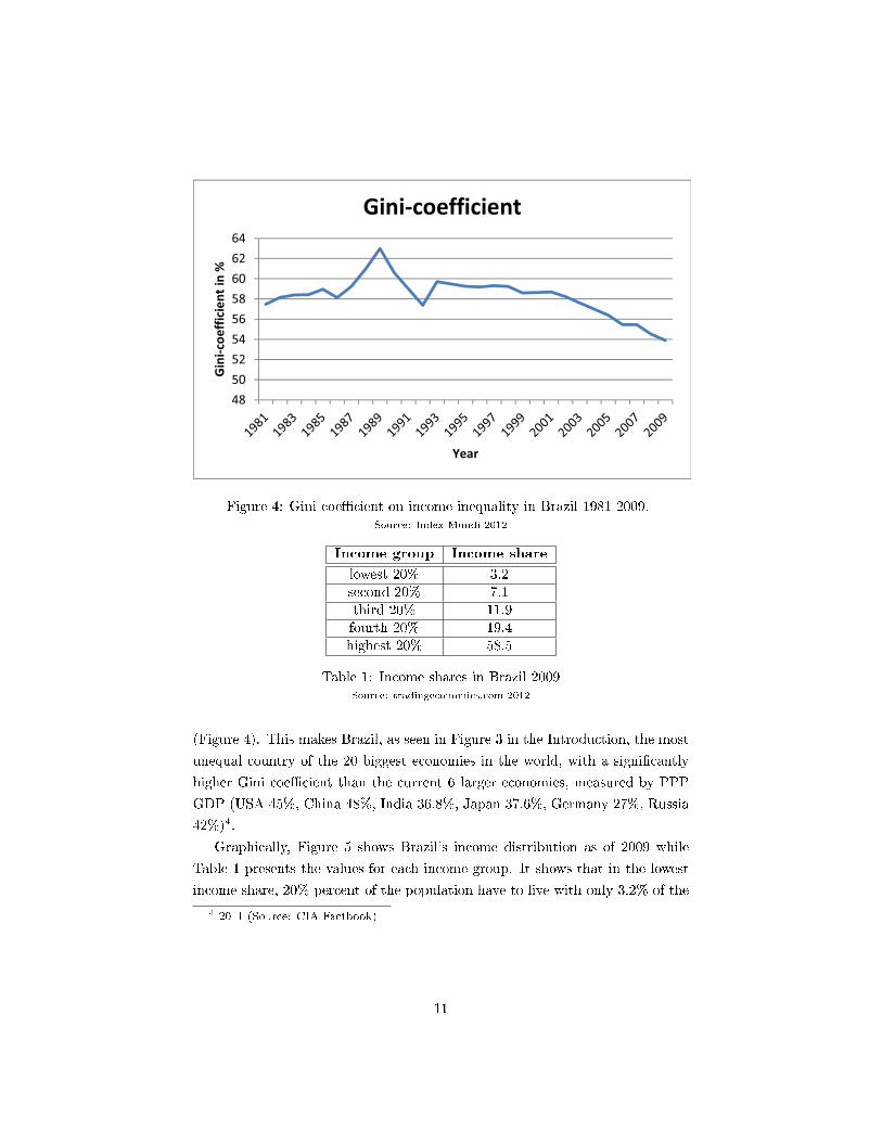
Income group Income share
lowest 20% 3.2second 20% 7.1third 20% 11.9fourth 20% 19.4highest 20% 58.5
Table 1: Income shares in Brazil 2009Source: tradingeconomics.com 2012
(Figure 4). This makes Brazil, as seen in Figure 3 in the Introduction, the most
unequal country of the 20 biggest economies in the world, with a signi�cantly
higher Gini coe�cient than the current 6 larger economies, measured by PPP
GDP (USA 45%, China 48%, India 36.8%, Japan 37.6%, Germany 27%, Russia
42%)4.
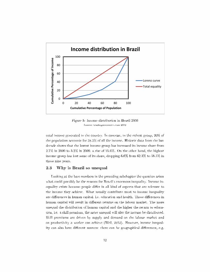
Graphically, Figure 5 shows Brazil's income distribution as of 2009 while
Table 1 presents the values for each income group. It shows that in the lowest
income share, 20% percent of the population have to live with only 3.2% of the4 2011 (Source: CIA Factbook)
11
�
��
��
��
��
���
� �� �� �� �� �������������� �������� ��
����������� ����������������
���������� ������������
���� ���
����� �������
Figure 5: Income distribution in Brazil 2009Source: tradingeconomics.com 2012
total income generated in the country. In contrast, in the richest group, 20% of
the population accounts for 58.5% of all the income. Historic data from the last
decade shows that the lowest income group has increased its income share from
2.7% in 2000 to 3.2% in 2009, a rise of 15.6%. On the other hand, the highest
income group has lost some of its share, dropping 6.6% from 62.3% to 58.5% in
those nine years.
2.3 Why is Brazil so unequal
Looking at the bare numbers in the preceding subchapter the question arises
what could possibly be the reasons for Brazil's enormous inequality. Income in-
equality exists because people di�er in all kind of aspects that are relevant to
the income they achieve. What usually contribute most to income inequality
are di�erences in human capital, i.e. education and health. Those di�erences in
human capital will result in di�erent returns on the labour market. The more
unequal the distribution of human capital and the higher the return to educa-
tion, i.e. a skill premium, the more unequal will also the income be distributed.
Skill premiums are driven by supply and demand on the labour market and
on productivity a worker can achieve (Weil, 2012). However, income inequal-
ity can also have di�erent sources: there can be geographical di�erences, e.g.
12
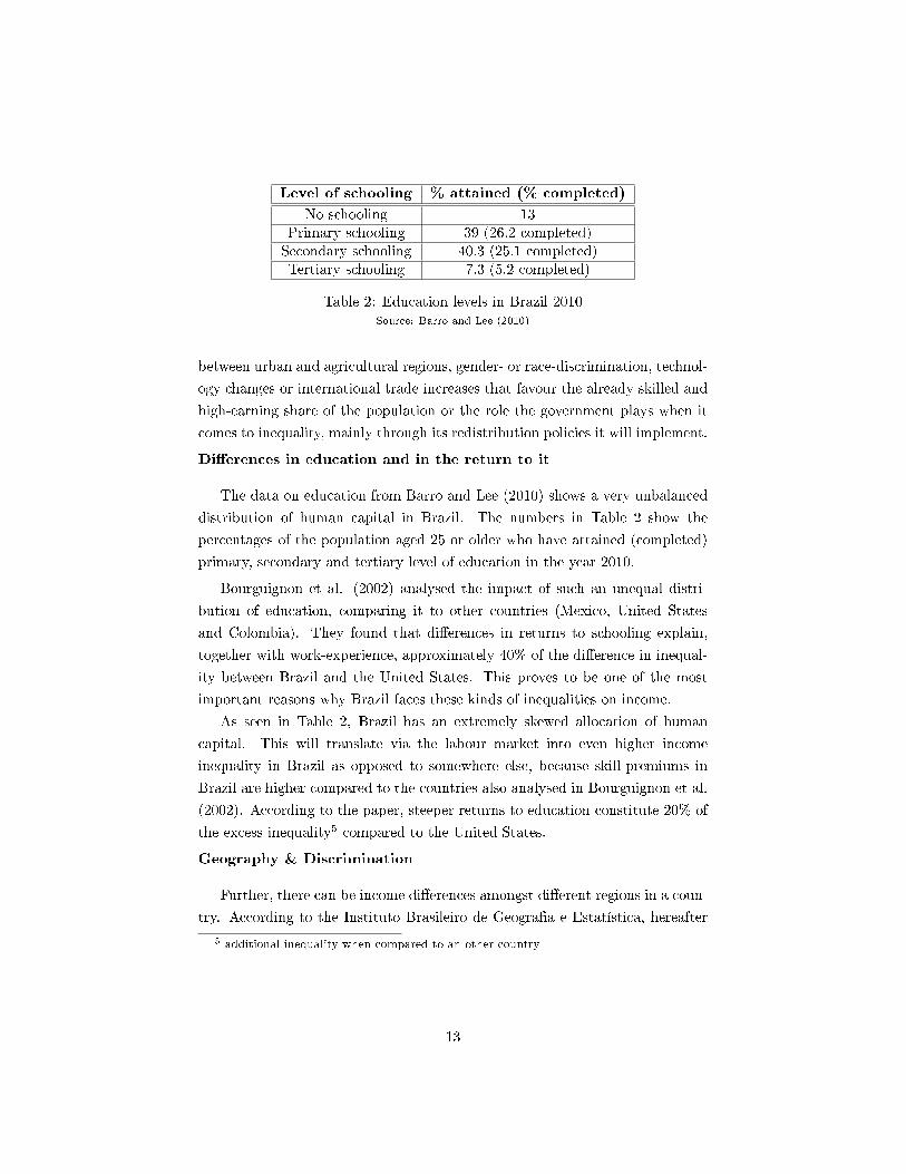
Level of schooling % attained (% completed)
No schooling 13Primary schooling 39 (26.2 completed)Secondary schooling 40.3 (25.1 completed)Tertiary schooling 7.3 (5.2 completed)
Table 2: Education levels in Brazil 2010Source: Barro and Lee (2010)
between urban and agricultural regions, gender- or race-discrimination, technol-
ogy changes or international trade increases that favour the already skilled and
high-earning share of the population or the role the government plays when it
comes to inequality, mainly through its redistribution policies it will implement.
Di�erences in education and in the return to it
The data on education from Barro and Lee (2010) shows a very unbalanced
distribution of human capital in Brazil. The numbers in Table 2 show the
percentages of the population aged 25 or older who have attained (completed)
primary, secondary and tertiary level of education in the year 2010.
Bourguignon et al. (2002) analysed the impact of such an unequal distri-
bution of education, comparing it to other countries (Mexico, United States
and Colombia). They found that di�erences in returns to schooling explain,
together with work-experience, approximately 40% of the di�erence in inequal-
ity between Brazil and the United States. This proves to be one of the most
important reasons why Brazil faces these kinds of inequalities on income.
As seen in Table 2, Brazil has an extremely skewed allocation of human
capital. This will translate via the labour market into even higher income
inequality in Brazil as opposed to somewhere else, because skill-premiums in
Brazil are higher compared to the countries also analysed in Bourguignon et al.
(2002). According to the paper, steeper returns to education constitute 20% of
the excess inequality5 compared to the United States.
Geography & Discrimination
Further, there can be income di�erences amongst di�erent regions in a coun-
try. According to the Instituto Brasileiro de Geogra�a e Estatística, hereafter5 additional inequality when compared to an other country
13
IBGE, which categorizes the country into 5 big regions, there are minimal dif-
ferentials in Gini coe�cients among those regions. The centre-west region, in-
cluding the capital Brasília, features the highest income inequality with a Gini
index of 55.4%. The lowest Gini value is found in the south region (48.9%),
which is also the smallest of the 5 big regions in Brazil.
Geographical di�erences in Gini coe�cients can also be looked at from an-
other perspective: One can distinguish between urban and rural areas. In 2005,
the urban Gini of Brazil was 60%, while the rural Gini was 54%, both being
signi�cantly over the average of other Latin American countries (50% for both
urban and rural Gini).6
Inequality can also have its sources from intended or unintended discrim-
ination, either in the labour market or directly through the government, e.g.
favouring a speci�c group of the population. Two forms of discrimination can
be of importance in Brazil: Gender discrimination and racial discrimination.
Barros (2002) published a study where racial discrimination contributed 5% to
the inequality from changes in labour earnings. Gender discrimination on the
other hand, had no contribution.
Historical distribution of assets and Opportunities
Economic inequality does not only show itself in income, but also in asset
distribution, especially the distribution of land (Deininger and Squire, 1998)).
The possession of land or other assets gives its owner the possibility to get a
return on them. Further, such a land-owner is favoured by �nancial institutions
to get his needed loans. Therefore, one can say that inequality in assets can
translate into income inequality and is thus one of the sources of it. Assuncao
(2006) calculated Land Gini coe�cients for Latin America and compared them
to Asia, Europe and the United States. Land distribution was the most unequal
in Latin America (83% Gini coe�cient), higher than in all other compared
regions of the world (Asia 52%, Europe 64%, United States 75%). This is
assumed to be one of the reasons why so many Latin American countries have
such unequal distributions of income, also seen in Figure 3.
Roemer (2000) proposed to look at the contribution of unequal opportunities
as a cause of inequality in earnings. He distinguished variables in to circum-
6 Source: http://media.routledgeweb.com/pdf/9781844076963/1_gini_on_urban_and-
ruralby_region_lac.pdf
14
stance and e�ort. E�ort is something that an individual can control and change,
as where circumstances cannot be controlled by the individual. Bourguignon
et al. (2007) took this approach and applied it to the case of Brazil. Variables
for circumstances were the father's and mother's education, the father's occu-
pation, the individual's race and region of birth. Those factors accounted for
10-37% of the Theil index on income inequality. It depends whether one only
accounts for direct e�ects of these uncontrollable variables or if one also takes
the indirect e�ects in to the estimation. It turns out that the education of both
parents is a signi�cant contributor to inequality, while the father's occupation
and race are less important but still signi�cant. This shows that social mobility,
i.e. moving up or down your income share group, is still pretty low. Improved
schooling rates and education parameters in the last 20 years (Barro and Lee,
2010) should have helped to improve social mobility and will do that further in
the future.
Government policies
In a �nal argument, I want to stress the importance of the role the government
has when it comes to inequality. First, one should look at the form of govern-
ment from a broader perspective, i.e. whether people in the society have a fair
chance to express their opinions and make them count in the political process,
for example through voting rights. This would be the case for a democratic
government that has been elected through a fair voting process. The opposite
of that would be a dictatorship government, where the population has no or
very limited power to express their political goals. Political economic theory
suggests that, facing the same amount of inequality, democracy-ruled states
have larger redistribution programs in place than dictatorships due to the pos-
sibility of either directly voting for more redistribution programs or by selecting
a government that promises more equalling policies (Barro, 2000). Section 3.2
focuses more on this mechanism and the possible e�ects redistribution programs
can have on economic growth. As the Brazilian population has lived under a
military dictatorship up until 1985, it is plausible that this period has been
a cause of the high inequality Brazil still su�ers today. But one would also
suspect inequality to be reduced after the introduction of democracy as voting
rights were expanded and people were able to vote for political parties in favour
of income-equalling measures. After analysing the form of government from a
purely democracy versus non-democracy standpoint, it can also be decisive to
di�er between di�erent political parties and their intention to reduce inequal-
15
ity. Mainly through the degree of redistribution programs, the political party in
power can a�ect the amount of inequality. In 2002, Luiz Inácio Lula da Silva,
hereafter Lula, became the �rst Brazilian president belonging to the Partido dos
Trabalhadores, hereafter Workers' Party or PT. With the intention to reduce
poverty rates and inequality, the government introduced a family redistribution
program called Bolsa familia which Lula hailed in a 2006 interview with The
Economist7 as �the most important income transfer programme in the world�.
A further measure to reduce inequality was a 25% rise in minimum wages. With
programs like the Bolsa familia and the raise of the minimum wage by Lula, if
implemented correctly, one should notice a decline in income inequality in the
last few years. As seen before, inequality has experienced a sharp decline in the
last decade. Whether this is caused by the stated policy measures or a�ected
by other e�ects, like improved education and health conditions, is di�cult to
tell and will be looked at empirically in Section 5. There I will include dummy
variables for democratically elected governments and for Workers' Party gov-
ernments in my regressions to �nd out the determinants of inequality and the
variables that e�ect economic growth.
3 Theoretical Channels on how growth can be
a�ected
In modern economic literature there are many constructed theories on how in-
equality can a�ect the economic performance of a given country. Barro (2000)
classi�ed them into four categories: credit-market imperfections due to asym-
metric information and the absence of legal institutions, the amount of redis-
tribution programs, sociopolitical unrest and possible di�erences in saving rates
among di�erent income classes. In the following subsections I will analyze the
four possible channels stated by Barro theoretically and add a few further chan-
nels that can be of any importance. In a second part I will apply those factors
to the case of Brazil and evaluate their importance.
7http://www.economist.com/node/5578770
16
3.1 Credit-market imperfections
Due to credit-market imperfections, people with no or little assets tend to not
receive loans and therefore often cannot invest in opportunities that would bring
them a positive return. This might be the case for investments in human capital.
Galor and Zeira (1993) explained that the di�erence in investing in human cap-
ital as opposed to physical capital is that the human capital is not transferable.
As a result, the marginal product of a human capital investment is declining
with the amount invested by a person. Physical capital on the other hand has a
constant return independent of the amount already invested. At �rst the return
on human capital is higher than on physical capital and thus the �rst amount
of investment will be dedicated to human capital. But as the marginal product
declines, there will be a point where the constant return on physical capital is
higher so that a person will only invest in physical capital from that point on.
In an economy where a poor person is not able to borrow from a bank or other
institutions, he will not be able to make an investment in human capital. This
situation of inequality cannot be economically e�cient as marginal products of
human capital investments are higher in the beginning as physical capital in-
vestments after the threshold point. A redistribution from the rich to the poor
would in that case raise the quantity and average productivity of investment.
Higher inequality through credit-market imperfections thus reduces the possible
economic output. Reasons for credit-market imperfections might be because of
imperfect law enforcement or insu�cient laws to protect the assets of debtors.
Those factors should improve though as an economy develops and therefore have
a higher impact on poor economies (Barro, 2000).
3.2 Redistribution programs
In a society with majority voting rights, there is usually a strong favour for
redistribution programs if the assets are heavily unequal distributed among the
individuals. This may involve explicit transfer payments or public-expenditure
programs with a progressive tax system (Barro, 2000). A bigger di�erence
between the mean and the median income will tend to bring more redistribution
as a result of the political process. More redistribution creates more economic
distortions as rich people will be discouraged to work more if more of their
income is redistributed or try to avoid those taxes. The individuals on the
17
receiving end of those redistribution payments also have fewer incentives to
put in more e�ort at work. These factors tend to retard average productivity
and lower investment which results in a negative e�ect on economic growth.
In short, a greater amount of inequality will provoke a greater redistribution,
so that initial inequality will reduce economic growth through the channel of
redistribution politics (Barro, 2000).
3.3 Sociopolitical unrest
High inequality tends to increase crime and other unproductive activities and
might even destabilize a country's institutions. Those actions are a waste of
potential economic resources and could, in the worst case, bring down the in-
vestment in an economy as property rights are threatened (Barro 2000). Perotti
(1995) also found that in more unequal societies individuals tend to engage in
more rent-seeking activities or manifestations of socio-political instability. High
inequality therefore is a cause of wasting resources and deterring potential in-
vestment and has thus a negative e�ect on economic growth.
3.4 Saving rates
By the assumption that individual saving rates rise with the level of income,
a redistribution of wealth or income from the rich to the poor would lower
the aggregate saving rate. In an at least partly closed economy that would
lower investment which would shift the economy into a lower steady state, thus,
reducing economic growth for the speci�c transition period from its original to
the new steady state in the neoclassical growth model by Solow (1956). Contrary
to the previous three possible channels, saving rates provide an explanation why
inequality could have a positive impact on economic growth.
3.5 Further channels
Besides the four channels presented above, there are a number of other possible
channels that might e�ect economic growth. De la Croix and Doepke (2002)
argue that fertility should be considered as an important channel. By the as-
18
sumption that poorer parents tend to have many children and thus, and through
the fact that they are poor, will invest only little in their education. Higher in-
come inequality will therefore increase the fertility di�erential between the rich
and the poor, which means that the amount of children with no or little edu-
cation increases. Consequently, this e�ect lowers the average education and the
average human capital endowments and therefore, lowers growth. De la Croix
and Doepke (2002) make the case in their paper that this fertility di�erential
e�ect accounts for most of the impact inequality has on growth. More general,
the relationship between income inequality and health has been looked at. Sub-
ramanian & Kawachi (2004) and Ram (2006) found a negative impact of income
inequality on general health in a society, especially signi�cant for the poorest
countries. Further, undesirable health conditions can translate into lower eco-
nomic performance which lowers economic growth. There is even evidence that
this channel might as well be active for economically advanced countries where
social standing has become more and more important. Marmot (2004) showed
that one's social standing can directly e�ect the person's health due to factors
like stress and anxiety.
3.6 Net e�ect
As seen in the previous subchapters, there are many possible channels on how
inequality might e�ect economic growth. Most of those channels have a negative
impact on subsequent growth, but there are also other channels which tend to
be the other way round, e.g. the e�ect that di�erent saving rates can have.
From a theoretical standpoint it is therefore almost impossible to estimate the
net e�ect that occurs when combining all the single channels. It might also be
necessary to analyze those channels in detail for any special case to get a more
plausible picture of the importance of each channel. Subsection 7 will thus be
a summary of how those possible channels could translate in the case of Brazil.
3.7 Situation in Brazil
When looking at possible channels that in�uenced Brazil the most, credit-
market imperfections should probably be the one channel emphasized the most,
especially in the pre-democracy era before 1985. During the period of military
19
dictatorship during 1964 until 1985 it is reasonable to presume some kind of
favouritism towards a speci�c group that was leaning towards the rulers of this
time. This alone might already be an inequality-augmenting fact, but further it's
realistic to assume this in-favour group had better access to the credit-market,
e.g. loans. After 1985 as institutions grew more reliable and democratic right
came in to place, the number of loans in general probably went up. Whether
it changed the situation for the poor with little or no assets to get their loans
for investing in mostly their human capital or simple machines for agricultural
activities is di�cult to tell. However, with the emergence of micro-credits in
the last couple of decades and the subsidizing of such micro-credits through the
government since 2005 to bring interests rates down to 8%8 it can be assumed
that today more poor people can have access to credit-market institutions than
in the past. Therefore, I would judge the channel of credit-market imperfections
as important for Brazil but with declining importance in the last three decades
and possible in the future as well.
Applying the logic from Chapter 3.2, considering the high income inequality
and the democratic situation in today's Brazil, one might guess that huge re-
distribution programs were in place to partly balance out the country's income.
Immervoll et al. (2005), though, provide facts that contradict that theory. At
the time of their study, the tax-system in Brazil had a very little equalising
e�ect on income inequality, mainly due to its regressive pension program. This
signalises that the channel is of lesser importance although the tax revenue as
percentage of GDP is at 39.9 9 which is a high number in international compari-
son. This can provoke economic distortions and ine�ciencies but high inequality
is unlikely the sole trigger for the high tax revenue number.
Political unrest in Brazil today is not an issue that could have huge e�ects
as a channel, even during and at the end of the period of military dictatorship
there is no evidence of civil war-like circumstances with highly explosive politi-
cal riots and excesses (Skidmore, 1990). Moreover, with the economic advances
the country experienced in the last decade, political unrest seems even more un-
likely. Although inequality has stagnated for a long period, wages for low-skilled
workers, pensions and entitlements for the poor have still risen in absolute terms.
This should also have an e�ect on poverty-based crime rates as the incentive8Source: 2011 press release by the Brazilian government ( http://www.brasil.gov.br/-
para/press/press-releases/august-1/brazil-expands-federal-microcredit-program-lowers-interest-rates/br_model1?set_language=en)
92011 est. (Source: CIA Factbook)
20
for doing something illegal, e.g. for stealing, has decreased because of better
outside opportunities, i.e. people who are considering illegal activities have now
more to lose than before. Sachsida et al. (2010) have explored the connection
between crime and inequality in Brazil and found that high inequality increases
criminal behaviour but found no evidence on a relationship between inequality
and strongly violent crimes. But again, it's very di�cult to distinguish whether
these criminal activities are induced by inequality or just absolute poverty lev-
els. On one hand, it's hard to believe that when, in a theoretical approach, all
people would have their income doubled over night (but prices on necessities
remain constant), thus leaving inequality exactly the same, that no one changes
his decision to enter in to illegal activities. On the other hand, several stud-
ies like Ravallion (2001) have showed that inequality and poverty numbers are
heavily correlated.
To my knowledge, no data on income-group speci�c saving rates exist for
the case of Brazil. But results from international research regarding the topic
suggest that saving rates tend to rise signi�cantly with income. Dynan et al.
(2004) collected data for households in the United States where at least one
member was aged 30-59. The results showed that the lowest income quintile
saves only 9% of their income, while the rate of the highest income quintile
is at 24.4%. It is plausible to assume a similar outcome in Brazil, especially
because the poor in Brazil are in absolute terms worse o� than in the United
States and have therefore even less room to generate savings. After looking
at the results from Dynan et al. (2004) and the suspicion that results could
very well be more extreme for Brazil, the channel of di�erent saving rates for
di�erent income groups can play a big role in the e�ect of income inequality on
economic growth. However, with the trend of globalization and with economies
getting more open to foreign investment, a country's saving rate has less e�ect
in determining the country's amount of investment which will help produce
economic growth.
With a rate of population living under the poverty line at 26%10 there exists
a considerable high number of people who can barely survive on their current
economic situation. Such extreme conditions can lead to a poverty trap (Baner-
jee and Du�o, 2011) caused by insu�cient nutrition or health conditions. The
person who expierences such a poverty trap �nds himself in a vicious cycle from
which he is not able to escape, e.g. not being healthy leads to an inability to102008 (Source: Index Mundi)
21
work, which prevents him to get the income needed to pay for adequate treat-
ment of his health condition. As high inequality can be a cause of poverty or
is at least strongly correlated to it, this channel could prove to be very impor-
tant. A person who experiences the situation of being in a poverty trap will not
contribute to any economic growth, so the more people that are able to escape
those conditions, the more people will particape in economic activities, which
will lead to higher economic growth.
From 1960 until 2000 Brazil experienced a sharp decline in fertility overall
(Potter et al., 2010), but the development was not evenly distributed among
di�erent income groups (Muniz, 2009). Fertility �rst declined for the upper
income groups, thus increasing the fertility di�erential between the rich and the
poor. But in the last decade covered by the research of Potter et al. (2010)
fertility has also started to decline for lower income groups which, together with
stagnating number of fertility for upper income groups, has decreased the fertil-
ity di�erential again. Therefore, one can conclude that inequality has a�ected
economic growth through the channel of fertility di�erential among the poor
and the rich more in the past than it does now. Still, it is also today a factor
that cannot be underestimated.
After analysing the importance of the di�erent possible channels, it is hard
to conclude which e�ects will have a dominating in�uence in the case of Brazil.
Alone from this qualitative analysis it is impossible to guess the net e�ect that
inequality has on growth. Therefore, in Section 5, the paper will assess the issue
empirically and try to call the e�ect the Gini coe�cient has on growth in the
subsequent period.
4 Empirical �ndings on the e�ect on growth
Economic literature is full of studies concerning the relationship between in-
equality, the level of economic development and the e�ect inequality has on
growth. A �rst part is dedicated to Kuznets' theory about the interaction be-
tween a country's GDP and its Gini coe�cient. Secondly, the recent �ndings
from cross-country growth regressions will be summarized which have resulted
in sometimes contradicting results. A �nal subchapter will conclude about the
problems and implications that occur while researching this topic.
22
4.1 Evidence of Kuznets curve
Kuznets (1955) said that during a country's economic development, inequality
�rst rises and after a while declines again. Hence, we should have graph with
the level of inequality as a function of the level of GDP per capita that shows
an inverted U-shape. His primary example was the shift from the low-income
agricultural sector to the high-income industrial sector but his theory can be
applied to any major innovation or new technology. Assuming that at the
beginning all people are in the same, low-income sector, inequality starts at a
low point. If now people start moving in to the high-wage sector, inequality
will rise as long as it is only a few workers that change the sector. With time
and more people adapting to the change, inequality will decrease again as most
of the people are now in the high-income sector and every worker that joins
this sector will from now on lower inequality in the whole society. Kuznets
hypothesis has been the basis for many economic researchers who tried to prove
or disprove his theory. One can either try to �nd evidence on a possible Kuznets
curve by looking at a single country over time or in a cross-country approach
at a speci�c time.
There are many single country studies on whether there is an evidence of a
Kuznets curve. To just quote two: Williamson (1985) found that during 1823-
1915 there is good evidence of a Kuznets curve in England and Wales, while
Piketty (2000) argues that wage inequality in France between 1901 until 1998
has been extremely stable with no evidence of a Kuznets curve. Deininger and
Squire (1998) investigated the occurrence of a Kuznets curve for 49 countries.
The only found 5 countries, including Brazil11, with a signi�cant Kuznets curve,
4 countries with a signi�cant U-shape curve contrary to Kuznets' prediction and
40 countries with no signi�cant association between inequality and income.
In a cross-country approach, Barro (2000) found out that the relation be-
tween the Gini coe�cient and a quadratic in log(GDP) is statistically signi�cant
in a panel of Gini coe�cients observed 1960, 1970, 1980 and 1990. His data im-
plies that the Gini values rise with GDP for values of GDP less than $1636 (1985
US dollars) and declines afterwards when considering economic development as
the only determinant of inequality. The R-squared values range from 0.12 to
0.22. Hence, although statistically signi�cant, the level of economic development
does not explain much of the variations in income inequality across countries.
After including several other variables such as secondary and higher schooling,11and Hungary, Mexico, Philippines, Trinidad
23
openness, democracy and rule-of-law indexes and dummies for Africa and Latin
America, Barro (2000) gets very high R-squared values that range from 0.63 to
0.74. Considering all those variables, the GDP peak where inequality declines
afterwards occurs at a value of $3320 (1985 US dollars).
4.2 Cross-country regressions
Apart from the simple relationship between GDP per capita and an inequality
measure such as the Gini coe�cient, economists are interested in the e�ect
that inequality has on subsequent growth. Section 3 provided the theoretical
channels on how growth can be a�ected by inequality, now I will focus on the
empirical results from cross-country regressions. Most of the research evaluating
the inequality e�ect on growth use 5 year averages for Gini coe�cients and
look at the e�ect it has in the subsequent time period, usually also 5 years.
Most papers look at growth as a function of investment, initial GDP, years of
schooling and the Gini index. Deininger and Squire (1998) di�erentiate also
between Income and Land Gini and use di�erent regional dummies in their
regressions. Barro (2000) includes several other variables such as government
consumption relative to the country's GDP, rule-of-law and democracy indexes,
fertility rate, in�ation rate and the growth rate of terms of trade. Forbes (2002)
uses a simpler model which only includes the variables initial GDP, the Gini
index, male and female education measures and a PPP index.
Deininger and Squire (1998) showed in their results that inequality reduces
income growth for the poor but not for the rich countries. They also found
that land distribution plays an important role, especially for poor countries,
where land inequality has a strong negative e�ect on long-term growth. The
regional dummies, e.g. for Latin American and African countries, included in the
regression turned out to be negative and highly signi�cant. Barro (2000), with
all variables stated above included, found little overall prove whether inequality
increases or decreases subsequent growth. However, if the fertility variable which
is positively correlated with inequality is omitted from the regression, there is
a negative overall e�ect on growth. Splitting the observations in to high and
low GDP observations, one can see that the e�ect of inequality on growth is
negative for values of per capita GDP below $2070 and then becomes positive.
Forbes' (2002) results are in contrast to the previous �ndings of Deininger and
Squire (1998), Barro (2000) and several other researchers. His results show a
24
signi�cant positive e�ect in the short-term which is robust in various settings
and models. Medium- and long-term e�ects tend to decrease and could even be
negative.
4.3 Implications and problems
As seen in the previous two subsections, there is no clear consensus among
researchers on whether the Kuznets curve is an empirical regularity and on the
e�ects of inequality on subsequent growth. These di�erences mostly do not stem
from di�erent theoretical interpretations, but from di�erent data sets, di�erent
statistical methods and di�erent time horizons.
The �rst source of di�erences is mainly due to di�erent data sets. All data
sets used before Deininger and Squire (1998) cannot be considered as fully high-
quality data material. Deininger and Squire (1998) may be better and more
comprehensive, but the number of observations is still quite small and results
can be skewed in one or the other direction when leaving out a few of those
observations. Barro (2000), Banerjee and Du�o (2003) and Forbes (2002) use
similar high-quality data sets but quite often di�er in the observations they
consider for their regressions. This makes it hard to compare those �ndings as
di�erences could very well be from the data choice itself. Better quality of data
today and in the future will help researchers �nd more precise and clear answers
on these questions.
A second source of potential di�erences are di�erent statistical methods and
models. Which variables are included in the regression will have an impact on
the predicted e�ect inequality has. Omitting just one variable might have the
e�ect to make inequality signi�cant in the given regression. This is a problem
that cannot be easily solved as there is no consensus among economists what
the real model is about. Each paper gives its own reasoning about why some
variables are and some are not included in the regression analysis.
A third and �nal implication when comparing those papers is that they
operate with di�erent time horizons. Most papers seem to agree that the overall
long-term e�ect of inequality on subsequent growth is negative and stronger for
poorer countries than for the rich ones. However, for short-term implications,
the support for a negative e�ect is less clear. Some, like Forbes (2002) argue
that for rich countries, the short-term e�ect is even positive.
Despite having di�erent methods, data sets and time horizons in their regres-
25
sions, researchers can broadly agree on a few subjects: First, short-term e�ects
of inequality on growth are usually more positive or less negative as compared to
medium- and long-term e�ects. Second, growth of low-income countries is more
negatively a�ected by inequality than growth of high-income countries. And
third, regional dummies for African and Latin American countries are in most
studies highly signi�cant variables in growth regressions as well as in regressions
that look for the determinants of inequality.
5 Regressions
In an empirical part, I want to see whether I can answer one or possible more of
the three following questions with the data I collected: Is there evidence in the
data for the last four and a half decades for an income inequality based Kuznets'
curve in Brazil? What else apart from the country's level of GDP determines
income inequality in Brazil? And �nally, what are the e�ects of income in-
equality and di�erent forms of government/politics on economic growth? I use
regression analysis technique as seen in Barro (2000) to measure the determi-
nants of inequality and the impact on growth, but I only include data from one
country, i.e. Brazil. The reason behind this strategy is the improved quality
and quantity of the data available and maybe the possibility to explain some
of the e�ects that were expressed in regional dummies in cross-country growth
regressions. With high-quality data available back to 1966, there is now nearly
half a century with consistent data to analyse these interesting questions.
In both regressions I use dummies for di�erent forms of governments and
politics. I include a dummy for democracy for the period after the end of the
military regime in 1985. This radical change in the people's participation in
politics could have had impacts both directly on inequality, maybe reducing a
certain favouritism towards a speci�c group, and impacts through the channel
�redistribution programs� on economic growth. During a time of dictatorship,
where there are no voting rights to the public, a high number in inequality
does not automatically translate into more redistribution programs towards the
poor as there are no possibilities to express this postulation in the political
process. However, the channel �sociopolitical unrest� might weaken the e�ect,
because governments, facing election or not, could fear that high inequality
brings up tensions in the public that could lead to a disempowerment of such a
26
government. The second dummy included in the regression is a dummy for the
current political party, the Workers' Party, which is in power since 2003. Luiz
Inácio Lula da Silva, known as Lula, was elected president in 2002 after winning
the election against Fernando Henrique Cardoso, the former centrist-president.
Lula was reelected for a second term in 2006 and ended his presidency in 2010.
Since 2010, fellow party-woman Dilma Rousse� is in charge of the country. Lula
and Rousse�, together, were in power for the last ten years, so it is particularly
interesting how these ten years leadership of the PT have a�ected inequality on
one hand and economic growth on the other hand.
5.1 Data set
For the following regressions, I use 5-year averages of the variables throughout
all regressions to cover the short- and maybe some medium-term e�ects. For
GDP data, I use the GDP per capita in US dollar from the Penn World Ta-
ble for all the years covered in the regressions. The Penn World Table is one
of the most used data sets when it comes to national-accounts data, provided
by the University of Pennsylvania. As a variable for physical capital I took
the Investment/GDP ratio, which is a common variable in growth regressions
(Source: EconomyWatch.com). For education parameters, I use the data from
the Barro-Lee dataset (Barro and Lee, 2010). There, I use average years of
schooling for every type (primary, secondary and tertiary) of education to de-
termine which level of education might in�uence the amount of inequality in
Brazil. For the growth regressions, I use the more general average years of
schooling number for all the population above the age of 25. Gini coe�cient are
taken from Deininger and Squire (1998) for the period of 1966 until 1980, which
can be considered high-quality data material, and calculated from yearly Gini
data from TradingEconomics.com for the time after 1980. Table 4 provides the
basic information about the data set used in the following subchapters.
27
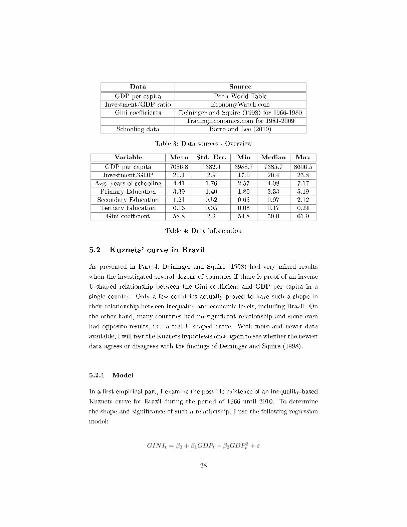
Data Source
GDP per capita Penn World TableInvestment/GDP ratio EconomyWatch.com
Gini coe�cients Deininger and Squire (1998) for 1966-1980TradingEconomics.com for 1981-2009
Schooling data Barro and Lee (2010)
Table 3: Data sources - Overview
Variable Mean Std. Err. Min Median Max
GDP per capita 7056.8 1382.4 3985.7 7385.7 8606.5Investment/GDP 21.1 2.9 17.0 20.4 25.8
Avg. years of schooling 4.41 1.76 2.57 4.08 7.17Primary Education 3.39 1.40 1.80 3.33 5.19Secondary Education 1.21 0.52 0.66 0.97 2.12Tertiary Education 0.16 0.05 0.06 0.17 0.24Gini coe�cient 58.8 2.2 54.8 59.0 61.9
Table 4: Data information
5.2 Kuznets' curve in Brazil
As presented in Part 4, Deininger and Squire (1998) had very mixed results
when the investigated several dozens of countries if there is proof of an inverse
U-shaped relationship between the Gini coe�cient and GDP per capita in a
single country. Only a few countries actually proved to have such a shape in
their relationship between inequality and economic levels, including Brazil. On
the other hand, many countries had no signi�cant relationship and some even
had opposite results, i.e. a real U-shaped curve. With more and newer data
available, I will test the Kuznets hypothesis once again to see whether the newest
data agrees or disagrees with the �ndings of Deininger and Squire (1998).
5.2.1 Model
In a �rst empirical part, I examine the possible existence of an inequality-based
Kuznets curve for Brazil during the period of 1966 until 2010. To determine
the shape and signi�cance of such a relationship, I use the following regression
model:
GINIt = β0 + β1GDPt + β2GDP2t + ε
28
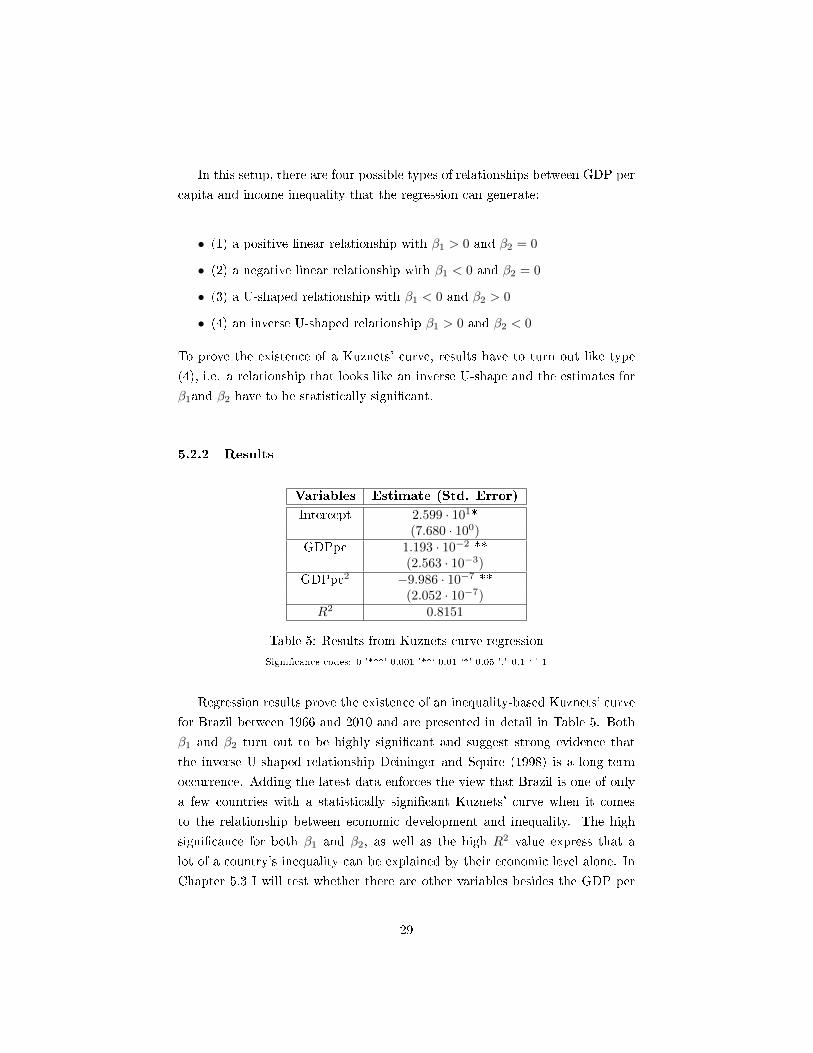
In this setup, there are four possible types of relationships between GDP per
capita and income inequality that the regression can generate:
• (1) a positive linear relationship with β1 > 0 and β2 = 0
• (2) a negative linear relationship with β1 < 0 and β2 = 0
• (3) a U-shaped relationship with β1 < 0 and β2 > 0
• (4) an inverse U-shaped relationship β1 > 0 and β2 < 0
To prove the existence of a Kuznets' curve, results have to turn out like type
(4), i.e. a relationship that looks like an inverse U-shape and the estimates for
β1and β2 have to be statistically signi�cant.
5.2.2 Results
Variables Estimate (Std. Error)
Intercept 2.599 · 101*(7.680 · 100)
GDPpc 1.193 · 10−2 **(2.563 · 10−3)
GDPpc2 −9.986 · 10−7 **(2.052 · 10−7)
R2 0.8151
Table 5: Results from Kuznets curve regression
Signi�cance codes: 0 '***' 0.001 '**' 0.01 '*' 0.05 '.' 0.1 ' ' 1
Regression results prove the existence of an inequality-based Kuznets' curve
for Brazil between 1966 and 2010 and are presented in detail in Table 5. Both
β1 and β2 turn out to be highly signi�cant and suggest strong evidence that
the inverse U-shaped relationship Deininger and Squire (1998) is a long-term
occurrence. Adding the latest data enforces the view that Brazil is one of only
a few countries with a statistically signi�cant Kuznets' curve when it comes
to the relationship between economic development and inequality. The high
signi�cance for both β1 and β2, as well as the high R2 value express that a
lot of a country's inequality can be explained by their economic level alone. In
Chapter 5.3 I will test whether there are other variables besides the GDP per
29
capita values that will prove to be statistically signi�cant, especially education
parameters.
Calculating with the results in Table 5, the tipping point occurs at $5973,
meaning income inequality rises before that level of GDP per capita and declines
afterwards. Barro (2000), in a cross-country study, found tipping points of $1636
(in 1985 dollars) and $3320 (in 1985 dollars) after �ltering out the estimated
e�ects of other variables than the GDP and its square. Deininger and Squire
(1998) calculated these peaks separately for each country. They found a value for
Brazil of $3117, which is about half of what my regression resulted in. This can
most likely be explained with the longer time horizon I used in my regressions
and the recent stronger decline in inequality in the last decade that probably
shifted the tipping point up in the time scale.
5.3 Determinants of Income Inequality
The previous subchapter showed that a lot of the variation of Brazil's in-
equality, measured by the Gini coe�cient, can be explained by its economic
level of development. This was expressed by highly signi�cant estimates that
enforce the view of a Kuznets' curve in the case of Brazil and an R2 value of
0.8151. Now in this section, it will be tested, whether there are other signi�cant
variables that can determine the level of inequality in Brazil.
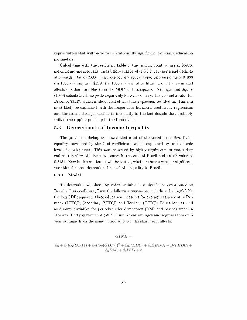
5.3.1 Model
To determine whether any other variable is a signi�cant contributor to
Brazil's Gini coe�cient, I use the following regression, including the log(GDP),
the log(GDP) squared, three education measures for average years spent in Pri-
mary (PEDU), Secondary (SEDU) and Tertiary (TEDU) Education, as well
as dummy variables for periods under democracy (DM) and periods under a
Workers' Party government (WP). I use 5 year averages and regress them on 5
year averages from the same period to cover the short-term e�ects:
GINIt =
β0 + β1log(GDPt) + β2(log(GDPt))2 + β3PEDUt + β4SEDUt + β5TEDUt +
β6DMt + β7WPt + ε
30
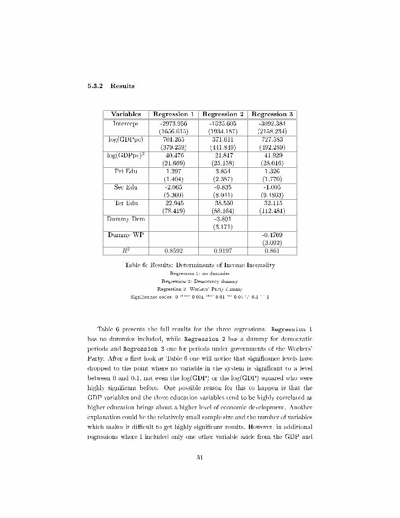
5.3.2 Results
Variables Regression 1 Regression 2 Regression 3
Intercept -2973.956 -1525.605 -3092.384(1656.615) (1934.187) (2158.234)
log(GDPpc) 701.265 371.611 727.583(379.259) (441.849) (492.289)
log(GDPpc)2 -40.476 -21.817 -41.929(21.669) (25.158) (28.016)
Pri Edu 1.397 3.854 1.326(1.404) (2.387) (1.770)
Sec Edu -2.065 -9.835 -1.005(5.360) (8.041) (9.4803)
Ter Edu -22.945 -38.550 -32.115(78.419) (88.164) (112.481)
Dummy Dem -3.891(3.171)
Dummy WP -0.4769(3.092)
R2 0.8592 0.9197 0.861
Table 6: Results: Determinants of Income InequalityRegression 1: no dummies
Regression 2: Democracy dummy
Regression 3: Workers' Party dummy
Signi�cance codes: 0 '***' 0.001 '**' 0.01 '*' 0.05 '.' 0.1 ' ' 1
Table 6 presents the full results for the three regressions. Regression 1
has no dummies included, while Regression 2 has a dummy for democratic
periods and Regression 3 one for periods under governments of the Workers'
Party. After a �rst look at Table 6 one will notice that signi�cance levels have
dropped to the point where no variable in the system is signi�cant to a level
between 0 and 0.1, not even the log(GDP) or the log(GDP) squared who were
highly signi�cant before. One possible reason for this to happen is that the
GDP variables and the three education variables tend to be highly correlated as
higher education brings about a higher level of economic development. Another
explanation could be the relatively small sample size and the number of variables
which makes it di�cult to get highly signi�cant results. However, in additional
regressions where I included only one other variable aside from the GDP and
31
GDP squared, I found that none of the here suggested variables is signi�cant.
GDP and GDP squared remain signi�cant in this one additional variable set-up,
but its signi�cance level drops when compared to the previous subsection. The
dummy variable introduced in Regression 2 for democratic periods turns out
to be negative. A �ve-year period under democratic ruling correlates with a
reduction of the Gini coe�cient of 3.891%. Regression 3 shows that periods
under the Workers' Party government have a similar, yet less strong e�ect. One
�ve year period under the ruling of the PT reduces the Gini index by 0.4769%.
However, the levels of signi�cance for the two dummies are quite low and one
should be very cautious to interpret these results. The reason for these low
signi�cance levels is again to be found at the low number of observations in the
regression.
5.4 E�ect on Growth
In a last empirical part, I will carry out growth regressions similar to works
like Barro (2000), but will do this only for the case of Brazil. The Gini coe�cient
will be included as an independent variable to determine the e�ect it has on
subsequent growth.
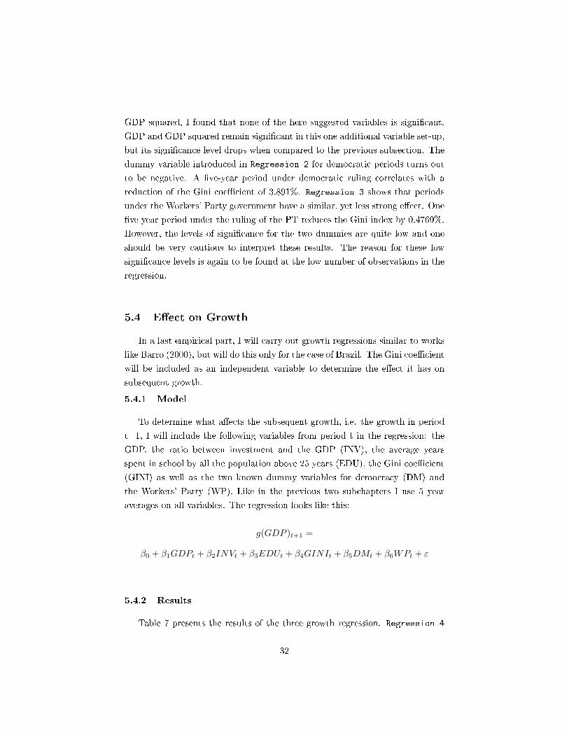
5.4.1 Model
To determine what a�ects the subsequent growth, i.e. the growth in period
t+1, I will include the following variables from period t in the regression: the
GDP, the ratio between investment and the GDP (INV), the average years
spent in school by all the population above 25 years (EDU), the Gini coe�cient
(GINI) as well as the two known dummy variables for democracy (DM) and
the Workers' Party (WP). Like in the previous two subchapters I use 5 year
averages on all variables. The regression looks like this:
g(GDP )t+1 =
β0 + β1GDPt + β2INVt + β3EDUt + β4GINIt + β5DMt + β6WPt + ε
5.4.2 Results
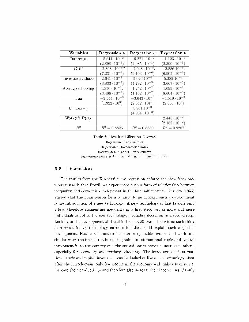
Table 7 presents the results of the three growth regression. Regression 4
32
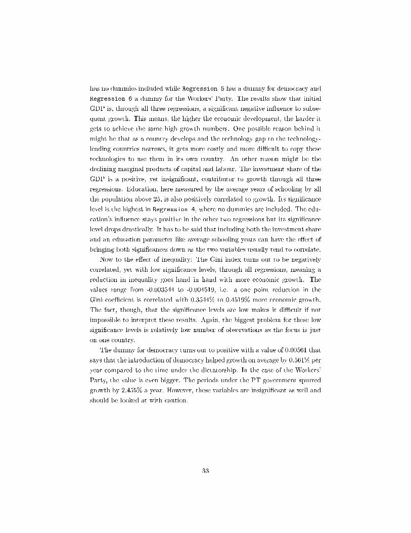
has no dummies included while Regression 5 has a dummy for democracy and
Regression 6 a dummy for the Workers' Party. The results show that initial
GDP is, through all three regressions, a signi�cant negative in�uence to subse-
quent growth. This means, the higher the economic development, the harder it
gets to achieve the same high growth numbers. One possible reason behind it
might be that as a country develops and the technology gap to the technology-
leading countries narrows, it gets more costly and more di�cult to copy these
technologies to use them in its own country. An other reason might be the
declining marginal products of capital and labour. The investment share of the
GDP is a positive, yet insigni�cant, contributor to growth through all three
regressions. Education, here measured by the average years of schooling by all
the population above 25, is also positively correlated to growth. Its signi�cance
level is the highest in Regression 4, where no dummies are included. The edu-
cation's in�uence stays positive in the other two regressions but its signi�cance
level drops drastically. It has to be said that including both the investment share
and an education parameter like average schooling years can have the e�ect of
bringing both signi�cances down as the two variables usually tend to correlate.
Now to the e�ect of inequality: The Gini index turns out to be negatively
correlated, yet with low signi�cance levels, through all regressions, meaning a
reduction in inequality goes hand in hand with more economic growth. The
values range from -0.003544 to -0.004519, i.e. a one point reduction in the
Gini coe�cient is correlated with 0.3544% to 0.4519% more economic growth.
The fact, though, that the signi�cance levels are low makes it di�cult if not
impossible to interpret these results. Again, the biggest problem for these low
signi�cance levels is relatively low number of observations as the focus is just
on one country.
The dummy for democracy turns out to positive with a value of 0.00561 that
says that the introduction of democracy helped growth on average by 0.561% per
year compared to the time under the dictatorship. In the case of the Workers'
Party, the value is even bigger. The periods under the PT government spurred
growth by 2.455% a year. However, these variables are insigni�cant as well and
should be looked at with caution.
33
Variables Regression 4 Regression 5 Regression 6
Intercept −5.611 · 10−2 −6.221 · 10−2 −1.123 · 10−1
(2.898 · 10−1) (2.985 · 10−1) (2.390 · 10−1)GDP −2.898 · 10−5* −2.948 · 10−5. −2.886·10−5.
(7.231 · 10−6) (9.103 · 10−6) (6.905 · 10−6)Investment share 2.641 · 10−4 5.026·10−4 5.285·10−4
(3.833 · 10−3) (4.792 · 10−3) (3.667 · 10−3)Average schooling 1.350 · 10−2. 1.252 · 10−2 1.099 · 10−2
(3.406 · 10−3) (1.162 · 10−2) (8.604 · 10−3)Gini −3.544 · 10−3 −3.643 · 10−3 −4.519 · 10−3
(1.922 · 103) (2.342 · 10)−3 (2.865 · 103)Democracy 5.961·10−3
(4.934 · 10−3)Worker's Party 2.445 · 10−2
(2.152 · 10−2)R2 R2 = 0.8826 R2 = 0.8850 R2 = 0.9287
Table 7: Results: E�ect on GrowthRegression 4: no dummies
Regression 5: Democracy dummy
Regression 6: Workers' Party dummy
Signi�cance codes: 0 '***' 0.001 '**' 0.01 '*' 0.05 '.' 0.1 ' ' 1
5.5 Discussion
The results from the Kuznets` curve regression enforce the view from pre-
vious research that Brazil has experienced such a form of relationship between
inequality and economic development in the last half century. Kuznets (1955)
argued that the main reason for a country to go through such a development
is the introduction of a new technology. A new technology at �rst favours only
a few, therefore augmenting inequality in a �rst step, but as more and more
individuals adapt to the new technology, inequality decreases in a second step.
Looking at the development of Brazil in the last 50 years, there is no such thing
as a revolutionary technology introduction that could explain such a speci�c
development. However, I want to focus on two possible reasons that work in a
similar way: the �rst is the increasing value in international trade and capital
investment in to the country and the second one is better education numbers,
especially for secondary and tertiary schooling. The introduction of interna-
tional trade and capital investment can be looked at like a new technology. Just
after the introduction, only few people in the economy will make use of it, i.e.
increase their productivity and therefore also increase their income. As it's only
34
a few that pro�t at the start, inequality will rise at �rst. Over the course of
time, more people will pro�t from trade or foreign investment, either directly
or through indirect e�ects, e.g. domestic suppliers will up their productivity
as well or will be able to pro�t from better infrastructure or already existing
contacts and relationships to enter the business too. The e�ect of education can
also be very similar. If only a low percentage of children get educated, through
the process of supply and demand, skill premiums will be high and wage di�er-
entials therefore huge. When more children enter the schooling system, human
capital endowments are more equally distributed. This will lower skill premi-
ums and have an equalling e�ect on wages. This equalling e�ect can mostly be
seen in Regressions 1 to 3 where increases in average secondary, but mainly
tertiary schooling attendance has a decreasing, yet insigni�cant, e�ect on the
country's Gini coe�cient.
In the analysis what determines income inequality, both dummies for democ-
racy and the Workers' Party were said to be decreasing inequality, with democ-
racy having a higher value. The introduction of democracy reduced the Gini
coe�cient by nearly 4 points in every 5-year period. Although the estimates
are of low signi�cance, looking at the theoretical channels and at some of the
facts about Brazil's inequality, this could make sense. Dictatorships tend to
favour certain individuals or groups being closely associated with the rulers,
which brings up high inequality. Democracy has therefore an equalling e�ect
or at least reduces the favouritism towards a speci�c group. A further e�ect to
consider when distinguishing a dictatorship and a democracy are voting rights.
Those voting rights should also have an equalling e�ect through the channel of
redistribution politics (Barro, 2000). Even though the value was not as high as
for democracy the years governed by the Workers' Party still had a decreasing
e�ect on income inequality. Bjornskov (2008) found similar results in world-wide
study that leftist leaning governments, like the Workers' Party, tend to reduce
inequality more than rightist leaning governments. Again, those results have to
be put in context. I regressed �ve-year period averages on the same �ve-year
period Gini averages, so the analysis is again very short-term. As more data
becomes available, medium- and long-term e�ects of various government parties
should be more clear and more signi�cant.
The growth regression results further emphasise the importance of education
to the country's growth in the last half century. While the population aged 25
and above in 1966 had only spent a little more than two and a half years in
school, it is in 2010 close to three times that amount. The question whether
35
income inequality contributed positively or negatively to subsequent economic
growth cannot be fully answered as signi�cance levels are too low. However,
from the insigni�cant negative estimate the Gini coe�cient has on growth and
from the qualitative analysis conducted earlier in the thesis, I would judge that
the in�uence of inequality in Brazil is negative on growth. It might well be that
short-term e�ects are close to zero or insigni�cant like in this paper's growth
regression, but it's very plausible to assume long-term e�ects of inequality to be a
negative contributor to growth, especially for low- and middle-income countries
in which Brazil was and is found in the last 50 years. The dummy variables
positive estimates for growth go well with one's intuition but are statistically
as well not signi�cant. But from the analysis before and also based on cross-
country studies it's probably right to say that dictatorships in general produce
lower economic growth rates than democracies in the same situation, which is
in line with economic and political theory and also with previous studies on
that matter. To judge the performance of the Workers' Party from a larger
perspective is di�cult as the party is only in charge for the last ten years and
results can be biased through business cycles and other distortions.
6 Conclusion
Inequality and its consequences on a country's economic performance are a
topic widely discussed and researched all around the world. This paper tried to
analyse the subject on a one country basis and showed that, for understanding
a countries inequality and the possible e�ects it might has, a precise qualitative
analysis is needed. It was able to show that an inequality-based Kuznets' curve
with the newest data is highly signi�cant and probably has a higher tipping
point than previously thought. It will be interesting to see whether this kind of
relationship that is quite rare will continue the same way as the last 50 years.
The paper also showed that it is practically impossible to get other signi�cant
variables apart from the country's level of GDP that determine inequality when
one includes the GDP variable in the regression. For further research, it is
possibly better to omit the GDP variable from the regression completely and
only work with other variables, like education and investment parameters, as
those are usually determining a country's level of GDP.
Another goal of the paper was to analyse the e�ect democracy had on both
inequality and economic growth in this one country set-up. It is reasonable to
assume from the qualitative analysis that democracy has decreased inequality
36
and increased economic growth as also the estimates from the regressions point
that way, unfortunately though with very low signi�cance levels. It was also the
�rst time, to my knowledge, that a paper analysed the e�ect of one particular
political party in such a one country regression system. Recent policies from
the Workers' Party and their goal to reduce poverty have made them a good
research subject to evaluate the growth performance under their regime and
whether they were able to reduce inequality. Poverty-reducing measures, like
the Bolsa familia, have de�nitely had an impact on poverty and thus also on
inequality as the sharp decline of the Gini coe�cient in the last decade showed.
It also has to be said that when it comes to inequality, there is often also a
normative element to the discussion, especially in a country like Brazil where still
a signi�cant amount of people live in poverty. Political and social preferences
play a role and have to be looked at aside e�ciency discussions. Brazil was, is
and will certainly be a case follow closely on this subject.
37
References
[1] A. Alesina and R. Perotti. Income distribution, political instability and
investment. European Economic Review, 40:1203�1228, 1996.
[2] J. Assuncao. Landreform and landholdings in brazil. World Institute for
Development Research Paper, 137, 2006.
[3] A. B. Atkinson. On the measurement of inequality. Journal of Economic
Theory, 2(3):244�263, 1970.
[4] A. B. Atkinson and F. J. Bourguignon. Handbook of Income Distribution:
Volume 1. Elsevier Science, 2000.
[5] A. V. Banerjee and E. Du�o. Inequality and growth: What can the data
say? Journal of Economic Growth, 8:267�299, 2003.
[6] A. V. Banerjee and E. Du�o. Poor Economics: A Radical Rethinking of
the Way to Fight Global Poverty. PublicA�airs, 2011.
[7] N. Barbosa. Latin america: Counter-cyclical policy in brazil: 2008-2009.
Journal of Globalization and Development, 1:1�11, 2010.
[8] R. J. Barro. Inequality and growth in a panel of countries. Journal of
Economic Growth, 5:5�32, 2000.
[9] R. J. Barro and J.-W. Lee. A new data set of educational attainment in
the world, 1950-2010. NBER Working Paper, (15902), 2010.
[10] R. Barros. Inequality in Brazil: Causes and Consequences. Rio de Janeiro:
Instituto de Pesqisa Economica Aplicada, 2002.
[11] N. Birdsall and R. Sabot. Opportunity Foregone: Education in Brazil.
Inter-American Development Bank, 1996.
[12] C. Bjornskov. The growth-inequality association: Government ideology
matters. Journal of Development Economics, 87:300�308, 2008.
[13] R. Bénabou. Inequality and growth. NBER Macroeconomics Annual, pages
11�73, 1996.
[14] F. J. Bourguignon, F. H. G. Ferreira, and P. G. Leite. Beyond Oaxaca-
Blinder: accounting for di�erences in household income distributions across
38
countries. Departamento de Economia, Ponti�ca Universidade Catolica do
Rio de Janeiro, Brazil, 2002.
[15] F. J. Bourguignon, F. H. G. Ferreira, and M. Menedez. Inequality of op-
portunity in brazil. Review of Income and Wealth, 53(4):585�618, 2007.
[16] A. Castello-Climent. Inequality and growth in advanced economies: an
empirical investigation. Journal of Economic Inequality, 8:293�321, 2010.
[17] F. A. Cowell and M.-P. Victoria-Feser. Robustness properties of inequality
measures. Econometrica, 64(1):77�101, 1996.
[18] C. Dagum. Income inequality measures. Encyclopedia of Statistical Sci-
ences, 2004.
[19] A. de Haan and S. Thorat. Addressing group inequalities: Social policies
in emerging economies' great transformation. European Journal of Devel-
opment Research, 24:105�124, 2012.
[20] D. de la Croix and M. Doepke. Inequality and growth: Why di�erential
fertility matters. American Economic Review, 93:1091�1113, 2003.
[21] A. Deaton. Analysis of Household Surveys. Baltimore MD: John Hopkins
University Press, 1997.
[22] K. Deininger and L. Squire. A new data set and measure of income in-
equality. World Bank Economic Review, 10:565�591, 1996.
[23] K. Deininger and L. Squire. New ways of looking at old issues: inequality
and growth. Journal of Development Economics, 57:259�287, 1998.
[24] K. E. Dynan, J. Skinner, and S. P. Zeldes. Do the rich save more? Journal
of Political Economy, 112(2):397�444, 2004.
[25] F. H. G. Ferreira, P. G. Leite, and J. A. Litch�eld. The rise and fall
of brazilian inequality: 1981-2004. World Bank Policy Research Working
Paper, 3867, 2006.
[26] K. J. Forbes. A reassessment of the relationship between inequality and
growth. The American Economic Review, 90(4):869�887, September 2000.
[27] D. Giles. Calculating a standard error for the gini coe�cient: Some further
results. Oxford Bulletin of Economic and Statistics, 66(3):425�433, 2004.
39
[28] D. Herzer and S. Vollmer. Inequality and growth: evidence from panel
cointegration. Journal of Economic Inequality, 2011.
[29] E. M. Hoover. The measurement of industrial localization. Review of
Economics and Statistics, 18:162�171, 1936.
[30] H. Immervoll, H. Levy, J. R. Nogueira, C. O�Donoghue, and R. B.
de Siqueira. The impact of brazil�s tax-bene�t system on inequality and
poverty. Ibero America Institute for Economic Research (IAI) Discussion
Papers, 117, 2005.
[31] S. S. . I. Kawachi. Income inequality and health: What have we learned so
far? Epidemiologic Reviews, 26:78�91, 2004.
[32] M. Kremer and D. L. Chen. Income distribution dynamics with endogenous
fertility. Journal of Economic Growth, 7(3):227�258, 2002.
[33] S. Kuznets. Economic growth and income inequality. American Economic
Review, 45:1�28, 1955.
[34] H. Li and H. fu Zou. Income inequality is not harmful for growth: Theory
and evidence. Review of Development Economics, 2:318�334, 1998.
[35] F. G. D. Maio. Income inequality measures. Journal of Epidemiol Com-
munity Health, 61:849�852, 2007.
[36] A. Malamud. A leader without followers? the growing divergence between
the regional and global performance of brazilian foreign policy. Latin Amer-
ican Politics and Society, 53(3):1�24, 2011.
[37] M. G. Marmot. The status syndrome : how social standing a�ects our
health and longevity. London: Bloomsbury, 2004.
[38] J. O. Muniz. Di�erential Reproduction, Poverty and the Dynamics of In-
equality in Brazil. PhD thesis, University of Wisconsin-Madison, 2009.
[39] T. Ogwang. Inter-country inequality in human development indicators.
Applied Economics Letters, 7:443�446, 2000.
[40] R. Perotti. Growth, income distribution and democracy: What the data
say. Journal of Economic Growth, 1:149�187, 1995.
[41] T. Piketty. Income inequality in france, 1901-1998. unpublished paper, 2000.
40
[42] J. E. Potter, C. P. Schmertmann, R. M. Assunca, and S. M. Cavenaghi.
Mapping the timing, pace, and scale of the fertility transition in brazil.
Population and Development Review, 36(2):283�307, 2010.
[43] R. Ram. Economic development and income inequality: An overlooked
regression constraint. Economic Development and Cultural Change, 43:425�
434, 1995.
[44] R. Ram. Further examination of the cross-country association between in-
come inequality and population health. Social Science & Medicine, 62:779�
791, 2006.
[45] M. Ravallion. Growth, inequality and poverty: Looking beyond averages.
World Development, 29(11):1803�1815, 2001.
[46] J. E. Roemer. Equality of Opportunity. Harvard University Press, 2000.
[47] A. Sachsida, M. J. C. de Mendonça, P. R. A. Loureiro, and M. B. S. Gutier-
rez. Inequality and criminality revisited: further evidence from brazil. Em-
pirical Economics, 39:93�109, 2010.
[48] A. Sen and J. E. Foster. On Economic Inequality. Oxford University Press,
1996.
[49] T. E. Skidmore. The Politics of Military Rule in Brazil, 1964-1985. Oxford
University Press, 1990.
[50] R. M. Solow. A contribution to the theory of economic growth. The Quar-
terly Journal of Economics, 70(1):65�94, 1956.
[51] H. Theil. Economics and Information Theory. Amsterdam: North-Holland,
1967.
[52] H. Theil. The measurement of inequality by components of income. Eco-
nomics Letters, 2:197�199, 1969.
[53] D. N. Weil. Economic Growth - 3rd Edition. Pearson Education Limited,
2012.
[54] J. Williamson. Did British Capitalism Breed Inequality? Boston: Allen &
Unwin, 1985.
41