Industry Effects of Monetary Transmission Mechanism in ...
41
Reserve Bank of India Occasional Papers Vol. 32, No. 2, Monsoon 2011 Industry Effects of Monetary Transmission Mechanism in India: An Empirical Analysis of Use-based Industries Sarat Dhal 1 This study evaluates the industry effects of monetary transmission mechanism in line with the literature on disaggregated approach to policy transmission mechanism. The study uses vector auto regression (VAR) model and monthly data from April 1993 to October 2011 pertaining to output growth of five use-based industries, call money rate and WPI inflation rate for evaluating the transmission mechanism. The generalised accumulated impulse response analysis from the VAR model showed that following a tight monetary policy shock, the output growth could be affected more for capital goods and consumer durables than basic, intermediate and consumer non-durable goods. Intermediate and consumer non-durable goods could show a relatively moderate transient response and transmission lag could be evident for the consumer non-durable goods. However, relatively wide asymptotic standard error bands associated with the impulse responses could be reflecting uncertainty in the impact of transmission mechanism. JEL classification : E52, L60 Keywords : Monetary policy, industry effects, vector auto regression Introduction In recent years, trends in the growth of industrial production in the Indian context have given rise to various concerns, notwithstanding the discussion over data quality and turbulent period of the global crisis. Should the industry sector be accorded policy attention by the authorities, especially from the perspective of monetary policy? How does monetary policy affect the industry sector? Answers to these questions, prima facie, cannot overlook some stylised facts. In the year 2011-12, the industry sector, comprising mining, manufacturing, and electricity, gas and water supply, accounted for 18.3 per cent of 1 Sarat Dhal is Assistant Adviser in the Department of Economic and Policy Research and currently working at the Center for Advanced Financial Research and Learning, Reserve Bank of India, Mumbai. The responsibility for the views expressed in the paper lies with the author only and not the organisation to which he belongs. The author is grateful to the anonymous refree for comments.
Transcript of Industry Effects of Monetary Transmission Mechanism in ...

Reserve Bank of India Occasional PapersVol. 32, No. 2, Monsoon 2011
Industry Effects of Monetary Transmission Mechanism in India:
An Empirical Analysis of Use-based Industries
Sarat Dhal1 This study evaluates the industry effects of monetary transmission mechanism in line with the literature on disaggregated approach to policy transmission mechanism. The study uses vector auto regression (VAR) model and monthly data from April 1993 to October 2011 pertaining to output growth of five use-based industries, call money rate and WPI inflation rate for evaluating the transmission mechanism. The generalised accumulated impulse response analysis from the VAR model showed that following a tight monetary policy shock, the output growth could be affected more for capital goods and consumer durables than basic, intermediate and consumer non-durable goods. Intermediate and consumer non-durable goods could show a relatively moderate transient response and transmission lag could be evident for the consumer non-durable goods. However, relatively wide asymptotic standard error bands associated with the impulse responses could be reflecting uncertainty in the impact of transmission mechanism.
JEL classification : E52, L60Keywords : Monetary policy, industry effects, vector auto regression
Introduction In recent years, trends in the growth of industrial production in the Indian context have given rise to various concerns, notwithstanding the discussion over data quality and turbulent period of the global crisis. Should the industry sector be accorded policy attention by the authorities, especially from the perspective of monetary policy? How does monetary policy affect the industry sector? Answers to these questions, prima facie, cannot overlook some stylised facts. In the year 2011-12, the industry sector, comprising mining, manufacturing, and electricity, gas and water supply, accounted for 18.3 per cent of
1 Sarat Dhal is Assistant Adviser in the Department of Economic and Policy Research and currently working at the Center for Advanced Financial Research and Learning, Reserve Bank of India, Mumbai. The responsibility for the views expressed in the paper lies with the author only and not the organisation to which he belongs. The author is grateful to the anonymous refree for comments.

RESERVE BANK OF INDIA OCCASIONAL PAPERS 40
GDP at factor cost at current prices, as compared with the shares of agriculture and services sectors at 17.2 per cent and 64.5 per cent, respectively. However, the industry sector played a dominant role in the Indian economy in various other ways including investment (or capital formation) activities, economy-wide gross output or aggregate economic transaction, inter-sectoral intermediate demand, merchandise trade, employment and bank credit in the organised sector. Firstly, the national accounts statistics (NAS) for 2010-11 showed that the industry sector accounted for 41.0 per cent of economy-wide gross domestic capital formation, closer to services sector’s share 51.0 per cent and substantially higher than the agriculture sector’s share 8.0 per cent. Secondly, the Input-Output transaction Table 2006-07 showed that the secondary sector led by industries accounted for 40 per cent of economy-wide gross output or economic transaction as compared with the shares of 47 per cent and 13 per cent for services sector and ‘agriculture and allied activities’, respectively. The secondary sector accounted for the bulk 58 per cent of aggregate inter-industry intermediate demand for goods and services, reflecting its backward and forward linkages with other sectors. Thirdly, according to the balance of payments (BOP) accounts 2011-12, merchandise and invisibles items accounted for 58.5 per cent and 41.5 per cent of India’s exports of goods and services in the current account, respectively. Exports of manufactured goods accounted for the bulk of merchandise exports with a share of 61.3 per cent. In 2011-12, imports of industrial inputs accounted for 51.0 per cent of India’s total merchandise imports and 73.5 per cent and 89.9 per cent of non-oil imports and non-oil and non-gold-silver imports, respectively. Fourthly, according to the NSSO Report on employment and unemployment survey 2009-10, there were 545 persons for every 1000 persons employed in non-agricultural activities. The industry sector accounted for 22 per cent of employment in the non-agricultural sector. Fifthly, industry sector comprising small, medium and large enterprises accounted for 45.8 per cent of gross non-food credit, leaving 12.2 per cent for agriculture and 42.0 per cent for other sectors, respectively. Finally, from the perspective of business cycle, a principal component analysis of GDP in terms of growth rate of broad sectors such as agriculture, industry and services reveals the crucial role of industry sector. The first principal component based on ordinary correlations could be associated with similar loadings (weights) to industry and services sectors (Annex 1).

INDuSTRy EFFECTS OF MONETARy TRANSMISSION MECHANISM41
The above stylised facts persuaded this study for analysis of monetary transmission mechanism for India’s industry sector. At this juncture, however, a mute question arises. Should the empirical analysis be confined to monetary implications for the industry sector at the aggregate level? This is an important issue because the industry sector is heterogeneous in nature in terms of product composition varying from salt and pepper to heavy transport machinery and aeronautics, agro-based products to resource based minerals, metal products and chemicals and used-based consumer durable and non-durable goods to basic goods, capital goods and intermediate goods. From this perspective, the study derives inspiration from the literature on disaggregated monetary transmission mechanism. According to this literature, it is important to understand how the effects of change in policy instruments pass through the economy, which sectors respond first to a policy innovation and whether the effects could be more pronounced in some sectors than others. A comparison of the monetary impact across different sectors may provide valuable information for policy purposes (Ganley and Salmon, 1997). In the study, the analysis is focused on monetary transmission mechanism for five use-based industries. using the standard VAR model and monthly data for the sample period April 1993 to October 2011, the study finds that the output growth response to monetary policy shock could be higher for consumer durables and capital goods industries than basic, intermediate and consumer non-durable goods. Intermediate goods industries could exhibit a muted response whereas consumer non-durables could exhibit moderate transitory response accompanied by lags in the transmission mechanism. These findings are expected to provide crucial information for policy purposes. The remainder of the paper is organised in five sections comprising review of literature, methodology and data, empirical findings and conclusion.
Section IIReview of Literature
The subject of monetary transmission mechanism has witnessed a paradigm shift over the years. For the first three to four decades during the post World War II period, economists adhered to the IS-LM type

RESERVE BANK OF INDIA OCCASIONAL PAPERS 42
aggregate macroeconomic model for evaluating the role of monetary policy in economic stabilisation through aggregate output growth and price inflation. Within this framework, it was postulated that policy induced changes in monetary variables could affect aggregate demand and consequently, the growth of economy-wide measure of output such as real gross domestic product and the inflation in the aggregate price index. This characterisation of the monetary transmission mechanism was later construed as a ‘black box’ view, as it did not tell about what happened in the interim in the transmission of policy shocks to the real economy (Bernanke and Gertler, 1995). Thus, the more recent literature on monetary transmission mechanism has embraced disaggregated analyses for a better understanding of how monetary variables affect various components of aggregate demand such as consumption, investment and trade and economic activities across firms, industries, sectors and regions within and across the nations. Studies in this tradition are inspired by the seminal works on asymmetric information, market imperfection and moral hazard by Stiglitz and Weiss (1981) and the credit channel comprising balance sheet channel (Bernake and Gertler, 1995) and the bank lending channel (Kashyap etal.1993 and Kashyap and Stein 1995). Also, several other studies emphasising on the heterogeneous characteristics of producing sectors pertaining to product composition, production technology reflecting upon the intensity of labour and capital inputs, financial structure of firms, openness to trade, wage contracts and flexibility in product prices have contributed to the growth of disaggregate analysis of monetary transmission mechanism [Ahmed (1987), Ahmed and Miller (1997), Angeloni, et al. (1995), Bernanke and Blinder (1988), Bernanke and Gertler (1995), Dale and Haldane (1995), David et al. (2000), Dedola and Lippi (2000), Ganley (1996), Ganley and Salmon (1997), Gertler and Gilchrist (1994), Gaiotti and Generale (2001), Hayo and uhlenbrock (1999), Kandil (1991), Kashyap et al. (1993), Kashyap and Stein (1995), Kretzmer (1989), Loo and Lastrapes (1998), Shelley and Wallace (1998), Peersman and Smets (2005)]. In the Indian context, studies in this tradition are scarce. Dhal (2012) provided an analysis of regional aspect of monetary transmission mechanism in terms of credit dispersion to states in the Indian context. Theoretical and empirical studies on disaggregated transmission mechanism focused on the industry sector provide various perspectives as discussed briefly in the following.

INDuSTRy EFFECTS OF MONETARy TRANSMISSION MECHANISM43
Firstly, the credit channel of transmission mechanism provides an explanation of differential effect of monetary transmission mechanism for firms and industries. Bernanke and Gertler (1995) provided explanation that monetary policy could affect the small firms differently from the large firms. The credit channel perspective on firm size implications for monetary transmission mechanism could be extended to the industry level analysis. Illustratively, basic, capital and consumer durable goods industries could be characterised with a concentration of large firms whereas intermediate and consumer non-durable goods could be characterised with several small firms. According to the credit channel, financial structure or leverage structure of small firms could be different from that of large firms. In this context, the financial accelerator theory of the monetary transmission mechanism states that asymmetric information between borrowers and lenders could give rise to an external finance premium, which typically depends on the net worth of the borrower. A borrower with higher net worth could be capable of posting more collateral and thereby, reduce its cost of external financing. As emphasised by Bernanke and Gertler (1989), the dependence of the external finance premium on the net worth of borrowers creates a “financial accelerator” propagation mechanism. A policy tightening will not only increase the cost of capital through the conventional interest rate channel, it will also lead to a fall in collateral values and cash flow, which will tend to have a positive effect on the external finance premium. Moreover, since collateral values and cash flows are typically low in a recession, the sensitivity of the external finance premium to changes in interest rates will be higher in recessions. Small firms, due to limited access to capital market and external borrowing, are likely to be more dependent on bank credit than large firms. Therefore, monetary policy involving contractions in bank credit and increased interest rate may affect expenditure by small firms more than the large firms. However, an alternative perspective is also maintained by several researchers. Due to large financing requirement at medium and longer horizons for investment activity, large firms may attach greater importance to credit and interest burden than smaller firms.

RESERVE BANK OF INDIA OCCASIONAL PAPERS 44
Secondly, the capital-labour intensity of production provides another explanation (Hayo and uhlenbrock, 1999, Berument etal., 2004, Ganley and Salmon, 1997). This perspective derives from Tobin’s (1960) work relating to money in the neoclassical growth model. In Tobin’s model, real money balance was postulated to affect capital-labour intensity in production, and thus, output growth. Deriving from this hypothesis, researchers argue that capital goods industries are likely to be associated with longer gestation lags, sufficiently large investment requirement and larger amount of credit with longer-maturity and higher interest rates than consumer goods. Thus, the causal nexus of monetary variables such as credit and interest rates with consumer goods and investment goods may not be similar. Berument etal. (2004) showed that an increase in interest rates affected the capital-intensive sectors more than labor-intensive ones. Similarly, Ganley and Salmon (1997) in a study of the uK economy showed that manufacturing, construction, distribution and transportation, exhibited the largest output responses to a monetary shock. Financial services and utilities responded relatively little to the monetary shock. The mining sector’s response was somewhat erratic and ambiguous and the agricultural sector’s response was insignificant.
Thirdly, there is an inventory adjustment perspective (Benito, 2002, Ehrmann and Ellison, 2002, Kashyap etal. 1994,Gertler and Gilchrist,1994). According to Ehrmann and Ellison (2002), the progress in production technology in terms of greater flexibility due to just-in-time production, lean manufacturing and improved inventory management enable firms to adjust their production levels more quickly, easily and at lower cost. Greenspan (2001) recognised that new technologies for supply-chain management and flexible manufacturing imply that businesses can perceive imbalances in inventories at an early age, virtually in real time, and can cut production promptly in response to the developing signs of unintended inventory building. Kashyap etal (1994) found for the uS that the inventory investment of firms without access to public bond markets was significantly liquidity-constrained during the 1981-82 and 1974-75 recessions, in which tight money also appeared to have played a role. Gertler and Gilchrist (1994) examined movements in sales, inventories, and short-term debt for small and

INDuSTRy EFFECTS OF MONETARy TRANSMISSION MECHANISM45
large manufacturing firms and confirmed that the effects of monetary policy changes on small-firm variables were greater when the sector as a whole was growing more slowly.
Fourthly, in terms of product characteristics, studies have examined the sensitiveness of durable goods to monetary policy as compared with non-durable goods (Mishkin 1976, Jung and yun 2005, Haimowitz, 1996, Kretzmer,1989, Ganley and Salmon,1997, Hayo and uhlenbrock, 2000 and Dedola and Lippi, 2000, Peersman and Smets,2002, Drake and Fleissig, 2010, Erceg and Levin, 2002). Mishkin (1976) addressed the neglected illiquid aspect of the consumer durable asset. He suggested that increased consumer liabilities are a major deterrent to consumer durable purchases and increased financial asset holdings a powerful encouragement. Monetary policy was found to have a strong impact on consumer durable expenditure through two additional channels of monetary influence. One, monetary policy affects the price of assets in the economy. Consumer financial asset holdings, thereby, affected expenditure on durables. Two, past monetary policy will have affected the cost and availability of credit, thus influencing the size of consumers’ debt holdings and hence consumer durable expenditure. Kretzmer (1989) suggested that unanticipated money could more likely display non-neutrality in the durable goods sector as agents spend unanticipated increases in their money holdings on goods which provide consumption services over time. Peersman and Smets (2002) showed the demand for durable products, such as investment goods, much more affected by a rise in the interest rate through the usual cost-of-capital channel than the demand for non-durables.
Fifthly, some industries may be producing more tradable goods than others catering to domestic demand. Here, the transmission mechanism could be influenced by the openness of the economy through monetary policy impact on exchange rate, capital flows and export and import prices (Berument etal. 2007). In a study of European countries, Llaudes (2007) found the tradable sector showing a higher degree of responsiveness to monetary policy shocks than the non-tradable sector and emphasised on the importance of industrial structure for the analysis of monetary policy.

RESERVE BANK OF INDIA OCCASIONAL PAPERS 46
Section IIIMethodology and Data
For the empirical analysis, we follow the literature and use standard vector auto regression (VAR) model. Due to the popularity of VAR model, we refrain from rehashing the model’s technical details. However, it is useful to highlight some applied issues relating to the VAR model for aggregated transmission mechanism as compared with the disaggregated model.
Firstly, for the aggregate transmission mechanism, researchers generally use a VAR model comprising three endogenous variables; an indicator of output growth, aggregate price inflation and the monetary policy variable, typically, the short-term interest rate. In principle, a VAR model is a reduced form of a structural model and residuals from the reduced form model cannot be considered as pure innovations. Accordingly, a meaningful analysis of impulse response and forecast error variance decomposition cannot be possible with a reduced form VAR model. It is in this context that researchers rely on orthogonalization of residuals from the reduced form VAR model. Orthogonalized innovations have two principal advantages over non-orthogonal ones: (i) because they are uncorrelated, it is very simple to compute the variances of linear combinations of them, and (ii) it can be rather misleading to examine a shock to a single variable in isolation when historically it has always moved together with several other variables. Or thogonalisation takes this co-movement into account. The greatest difficulty with orthogonalisation is that there are many ways to accom plish it, so the choice of one particular method is not innocuous. Researchers, however, often rely on Choleski factorization involving a lower triangular variance-covariance matrix of VAR residuals for deriving orthogonal shocks to the endogenous variables. The Choleski decomposition is sensitive to the ordering of variables in the VAR model when residuals are correlated. Studies on standard monetary transmission mechanism prefer output, inflation and interest rate variables appearing in order. In this way, the orthogonal innovations are justified with a structural identification of shocks to variables based on macroeconomic postulates such as technology shock driving output

INDuSTRy EFFECTS OF MONETARy TRANSMISSION MECHANISM47
growth, Philips curve describing inflation and output relationship and a monetary policy reaction function associated with output growth and inflation. In the case of disaggregated model involving more than three variables and more than one sectoral output indicators in particular, structural identification of shocks becomes extremely complicated and the straightforward Choleski factorization may not be meaningful. Illustratively, for a VAR model with seven variables comprising interest rate, inflation, and output growth of five use-based industries, the ordering choice becomes complicated with respect to which industry sector should precede or follow other sectors. On the statistical ground, one could find a solution through Granger’s causality among the output indicators. However, such causal ordering may not be consistent with the real world and the underlying technological relationship among producing sectors. In this context, we followed Pesaran and Shin (1998) who suggested that the generalized impulse response analysis, which is free from ordering of variables in the model, could provide a meaningful alternative to impulse response analysis.
Secondly, a peculiar feature of time series models such as the VAR pertains to its sensitivity to measurement of variables, data frequency, and the sample period. In the Indian context, monetary policy works through both quantity (liquidity management) and interest rate channels. Both effects are expected to affect the interbank call money rate in the same direction. Illustratively, a tight liquidity and an increase in the short-term policy rate such as the repo rate are expected to push up the call money rate and vice versa for easy liquidity and decline in the repo rate. For this purpose, we use monthly data for the weighted average interbank call money rate as the policy variable. The aggregate price variable is measured by year-on-year WPI inflation rate based on monthly data2. Similarly, the monthly data on output variables are used for deriving annualised or year-on-year growth rate of seasonally adjusted index of industrial production for five use-based industries. There are two principal reasons for using output growth and inflation rate variables. First, there is an information perspective relating to
2 The year-on-year inflation and output growth rates are defined as Log(Pt/Pt-12)*100 and Log(yt/yt-12)*100, respectively, where P and y refer to price and industrial production indices and Log denote for natural logarithm.
RESERVE BANK OF INDIA OCCASIONAL PAPERS 48
economic agents’ consumption, investment and production decisions and expectation formation process. The official source in India like the Central Statistical office releases monthly data on price and production indices in levels as well as year-on-year percentage increases. However, the year-on-year percentage increase in WPI index, i.e., inflation rate and the year-on-year percentage increase in industrial output indices or growth rates contribute to the headline news. From this perspective, it makes sense to emphasise that economic agents’ behavior and expectations could be influenced by information that is available, interpreted and understood. Secondly, the rate variables enable us to work with a VAR model comprising stationary variables. In our case, we found the variables stationary based on ADF and PP unit root tests. The empirical exercise with level variables (after long transformation of the price and output indices) will have to contend with non-stationary variables and require vector error correction and co-integration (VECM) model. However, the VECM model may involve multiple long-run co-integrating relationships among the variables, requiring identification of the multiple equilibrium trajectories in line with theoretical postulates, which may not be unique. Thus, it is useful to consider a VAR of stationary variables when the purpose is to understand the dynamic interaction among the variables. Moreover, the VAR model is also capable of reflecting upon the short-run and medium-longer horizon responses of variables to various types of shocks.
Thirdly, for a VAR model, the common lag length for the endogenous variables assumes critical importance. In this context, empirical studies often have to contend with alternative scenarios deriving from different lag selection criteria. Like other studies, we also faced difficulties in this regard. Some lag selection criteria like Schwartz Information Criterion (SIC) and Hannan and Quinn (HQ) criteria show lower lags (in our case 2 to 3 months) while others including Likelihood ratio(LR), adjusted LR and Akaike’s Final prediction Error (FPE) show higher lags (in our case 13 months). A lower lag length, however, could not ensure VAR residuals free from serial autocorrelation problem, especially, of first order which is a serious problem for statistical modeling. According to Lutkepohl etal. (2006), the lower lag length in this context could be inadequate to capture the underlying dynamic interaction among the

INDuSTRy EFFECTS OF MONETARy TRANSMISSION MECHANISM49
variables in the VAR model. On the other hand, a model with a higher lag length, though appropriate to capture the underlying dynamic interaction among the variables, could suffer from over parameterisation and efficiency. Nevertheless, most of the empirical studies in the transmission mechanism literature prefer full lag length, i.e., 4 to 5 lags for quarterly data and 12 to 13 lags for monthly data. Thus, in our study based on monthly data, we preferred 13 lags for the models in line with AIC and the empirical tradition.
Fourthly, the period-by-period impulse responses may appear obscure and lack smoothness due to large number of lags and high frequency monthly data. In this context, given the purpose of assessing the total impact of monetary policy shocks on output growth and inflation over different shorter and medium term horizons, an alternative approach entails accumulated impulse responses over different forecast horizon for the VAR model (Lutkepohl, 1990). We examined the cumulative impulse response over the time horizon spanning 1 to 60 months (five year) as this is consistent with the business cycle literature which maintains a typical business cycle spanning a period 2 to 5 years.
Section IV
Empirical Findings For the empirical analysis, we adopted a structured approach by estimating the VAR model with alternative combinations of endogenous variables and some exogenous variables in order to provide robustness to the findings. Before moving to the empirical findings, we bring some further facts about the use-based industries in order to facilitate the analysis and interpretation of the industry effects of monetary transmission mechanism. Firstly, the weights assigned to different use-based industries and the product compositions within each industry group provide some interesting insights. In the construction of index of industrial production, the highest weight is given to basic goods (46 per cent), followed by consumer non-durables (21 per cent), intermediate goods (16 per cent), capital goods (9 per cent) and consumer durables (8 per cent). Annex 2 shows top fifteen products in each user-industry group along with their weights. The distribution of weights reflects the concentration of

RESERVE BANK OF INDIA OCCASIONAL PAPERS 50
activities across the industry groups. Basic goods and consumer durables sectors show higher concentration of weights. This is reflected in top fifteen items accounted for 82 per cent, and 90 per cent of the respective sector’s weight whereas these figures stood at 64 per cent, 55 per cent and 66 per cent, respectively for capital goods, intermediate goods and consumer non-durables (Annex 2). In the basic goods group, two most important items were mining minerals (31 per cent) and electricity (23 per cent) – the utility sector mostly under the public sector, accounting for more than fifty per cent of the basic goods sector and a fifth of the total industry sector’s weight. Secondly, the growth dynamics of use-based industries showed that during the sample period the mean growth rate was highest for the consumer durables followed by capital goods, intermediate goods, consumer non-durables and basic goods (Table 1). In terms of volatility, i.e., standard deviation of growth rate, capital goods were most volatile followed by consumer durables, consumer non-durables, intermediate goods and basic goods. The volatility in industry output growth was also corroborated by maximum and minimum growth rates, reflecting sharper fluctuations in capital goods and consumer durables than other sectors.
Table 1: Summary Statistics of Industry Growth Rate
ZBGS ZKGS ZIGS ZCDGS ZCNDGS ZQS
Sector Weight 46 9 16 8 21 100
Mean 5.88 11.70 7.19 14.40 6.16 7.50
Median 5.62 9.89 6.68 13.65 5.63 7.10
Maximum 15.21 62.15 27.08 56.63 33.82 20.40
Minimum -2.18 -26.58 -7.72 -17.76 -20.75 -7.25
Std. Dev. 3.46 15.40 5.51 11.97 6.86 4.58Weighted contribution to overall Industry sector’s growth
36 14 15 17 18 100
Third, the weighted contribution of use-based industries to the overall industry sector’s growth provides another interesting insight.
INDuSTRy EFFECTS OF MONETARy TRANSMISSION MECHANISM51
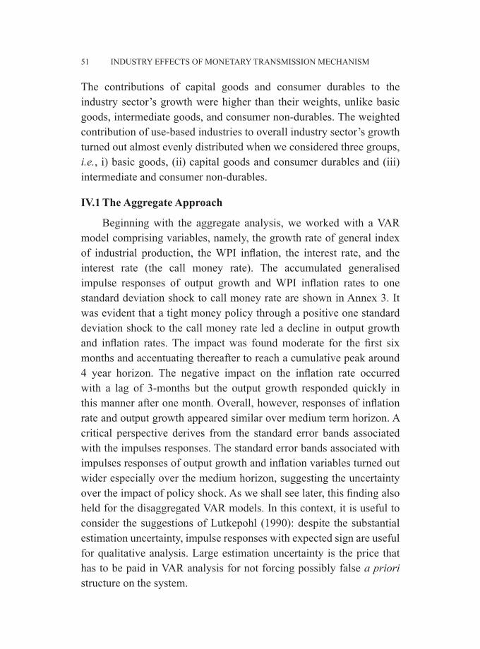
The contributions of capital goods and consumer durables to the industry sector’s growth were higher than their weights, unlike basic goods, intermediate goods, and consumer non-durables. The weighted contribution of use-based industries to overall industry sector’s growth turned out almost evenly distributed when we considered three groups, i.e., i) basic goods, (ii) capital goods and consumer durables and (iii) intermediate and consumer non-durables.
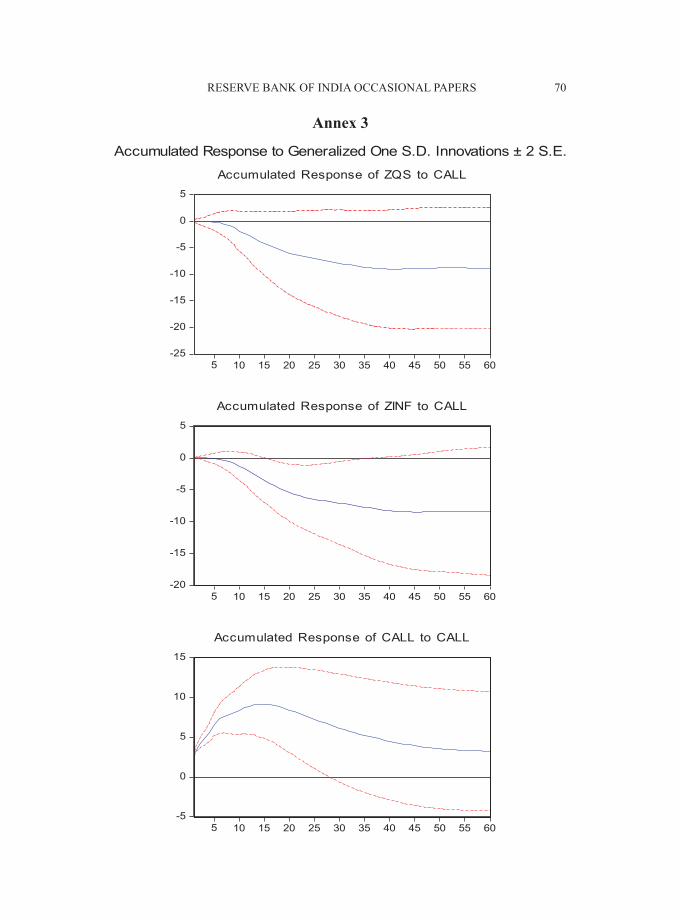
IV.1 The Aggregate Approach
Beginning with the aggregate analysis, we worked with a VAR model comprising variables, namely, the growth rate of general index of industrial production, the WPI inflation, the interest rate, and the interest rate (the call money rate). The accumulated generalised impulse responses of output growth and WPI inflation rates to one standard deviation shock to call money rate are shown in Annex 3. It was evident that a tight money policy through a positive one standard deviation shock to the call money rate led a decline in output growth and inflation rates. The impact was found moderate for the first six months and accentuating thereafter to reach a cumulative peak around 4 year horizon. The negative impact on the inflation rate occurred with a lag of 3-months but the output growth responded quickly in this manner after one month. Overall, however, responses of inflation rate and output growth appeared similar over medium term horizon. A critical perspective derives from the standard error bands associated with the impulses responses. The standard error bands associated with impulses responses of output growth and inflation variables turned out wider especially over the medium horizon, suggesting the uncertainty over the impact of policy shock. As we shall see later, this finding also held for the disaggregated VAR models. In this context, it is useful to consider the suggestions of Lutkepohl (1990): despite the substantial estimation uncertainty, impulse responses with expected sign are useful for qualitative analysis. Large estimation uncertainty is the price that has to be paid in VAR analysis for not forcing possibly false a priori structure on the system.

RESERVE BANK OF INDIA OCCASIONAL PAPERS 52
IV.2 Disaggregated Models
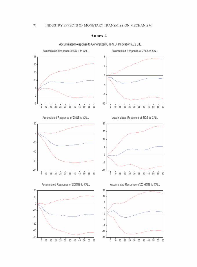
Moving to the disaggregated model, we considered first the VAR model (Model 1) comprising six variables, the interest rate and the output growth rates of five use-based industries. The impulse responses of sectoral output growth to call money rate shock is shown in Annex 4 and summarised in Table 2. Here, a couple of interesting insights emerged. One, a decline in the output growth following the tight money policy was associated with basic, capital, intermediate and consumer durable goods. However, consumer non-durables showed a transmission lag as the decline in output growth occurred after 8 months. Two, different sectors showed different peaks and maximum adverse impact due to the tight money policy shock. The maximum adverse impact was observed for the capital goods followed by consumer durables, basic goods, consumer non-durables and intermediate goods. Three, the peak period of cumulative maximum adverse impact (after which the policy shock faded away with no adverse impact) occurred over the period of 3-year horizon for consumer durables, followed by capital goods (2-years) and basic goods (one and half year). Intermediate goods and consumer durables were associated with moderate impact for shorter horizon of about a year.
Table 2: Impact of One Standard deviation Shock to Call Rate: Accumulated Responses of Output growth (Model without Inflation Rate)
Period ZBGS ZKGS ZIGS ZCDGS ZCNDGS1 -0.31 -0.81 -0.12 -0.07 0.266 -0.76 -6.15 -0.37 -5.36 1.777 -1.17 -7.09 -0.35 -7.53 2.208 -1.46 -8.19 -0.26 -9.28 2.4810 -2.08 -11.69 -0.61 -11.62 1.3112 -2.66 -15.40 -0.15 -14.19 0.5413 -2.54 -17.07 0.18 -14.70 -0.3718 -3.29 -23.73 1.82 -16.81 -1.9620 -3.21 -25.71 2.48 -16.55 -2.4025 -3.08 -27.29 3.70 -16.70 -1.7837 -1.80 -25.57 3.14 -18.91 0.5660 -1.35 -21.06 5.45 -15.37 1.24Generalised Impulse

INDuSTRy EFFECTS OF MONETARy TRANSMISSION MECHANISM53
IV.2.1 Model with Aggregate Price Inflation
In the Model 1, we did not include the inflation rate. However, monetary policy can affect inflation expectation and consequently, aggregate demand and supply conditions and real activity. Thus, we moved to the VAR model (Model 2) with WPI inflation as an endogenous variable in addition to the interest rate and sectoral output growth variables. The impulse responses of sectoral output in response to tight money policy shock are shown in Annex 5 and summarised in Table 3.
Table 3: Impact of One Standard deviation Shock to Call Rate: Accumulated Responses of Output growth and inflation rate
(Model with WPI Inflation Rate as an endogenous variable)Period ZINF ZBGS ZKGS ZIGS ZCDGS ZCNDGS
1 0.00 -0.37 -0.82 -0.09 0.05 0.17
8 -1.73 -2.25 -7.88 -0.94 -10.23 2.28
12 -3.47 -4.18 -14.93 -1.55 -16.91 -0.09
31 -8.64 -8.81 -29.16 -2.77 -32.02 -4.50
33 -8.78 -8.95 -29.39 -3.40 -33.54 -4.30
38 -8.88 -8.58 -30.44 -4.56 -35.54 -4.15
40 -8.83 -8.52 -30.00 -4.82 -35.85 -3.99
41 -8.77 -8.49 -29.98 -4.78 -36.06 -3.77
60 -8.76 -8.05 -23.94 -2.91 -31.60 -2.38
Generalised Impulse
The empirical findings from the Model 2 show some similarity as well as some notable departures from the Model 1. One, basic goods, capital goods, consumer durables and intermediate goods showed a decline in output growth following tight money policy shock while consumer non-durables showed a transmission lag. Moreover, consumer durables and capital goods were affected more than the three other sectors. Two, a comparison of the Model 2 (with inflation) with the Model 1 (without inflation) showed that all five use-based industries witnessed an accentuation of the maximum adverse impact on output growth due to tight money policy shock in the presence of inflation variable. Three, some sectors witnessed a significant increase in the time horizon for the adverse output

RESERVE BANK OF INDIA OCCASIONAL PAPERS 54
effect; from 18 months (Model 1) to 33 months (Model 2) for basic goods and from 10 months to 40 months for the intermediate goods sector. Similarly, consumer non-durables also showed an increase in the time horizon of declining output response from one year (between 8-20 months) to two year horizon (between 8-31 months). Four, consumer durables witnessed maximum impact followed by capital goods in Model 2 unlike the capital goods being impacted more than consumer durables in the Model 1.
IV.2.2 Model with Exogenous Supply Shocks
In the Indian context, the sharp fluctuation in inflation condition often occurs due to supply shocks arising from the movement in the prices of oil and food commodities. Empirical studies generally consider such supply shocks as exogenous in nature as they could not be affected by policy intervention. From this perspective, we estimated VAR model (Model 3) with oil price inflation and food price inflation as exogenous variables. The impulse responses of sectoral output growth to call money rate shock are summarised in Annex 6 and Table 4. A couple of notable findings emerged from the comparison of Model 3 with Model 2. One, all sectors witnessed a moderation in the maximum adverse output effect due to tight money policy shock in the presence of oil price and food price inflation variables. This suggested that supply shocks may not accelerate the monetary impact on real activity. Two, at the same time, Model 3 showed consumer durables with higher impact than capital goods, similar to Model 2. However, the difference between the magnitudes of maximum impact for these two sectors in Model 3 was significantly higher than the Model 2. In other words, a model without controlling for supply shocks could show some overreaction in the growth response of capital goods to policy shock. This is a critical finding because capital goods have implications for overall capacity building and long-run growth trajectory of the economy.
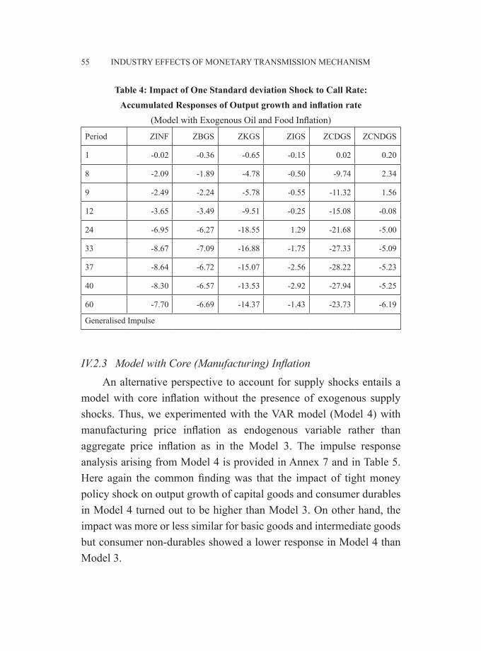
INDuSTRy EFFECTS OF MONETARy TRANSMISSION MECHANISM55
Table 4: Impact of One Standard deviation Shock to Call Rate: Accumulated Responses of Output growth and inflation rate
(Model with Exogenous Oil and Food Inflation)
Period ZINF ZBGS ZKGS ZIGS ZCDGS ZCNDGS
1 -0.02 -0.36 -0.65 -0.15 0.02 0.20
8 -2.09 -1.89 -4.78 -0.50 -9.74 2.34
9 -2.49 -2.24 -5.78 -0.55 -11.32 1.56
12 -3.65 -3.49 -9.51 -0.25 -15.08 -0.08
24 -6.95 -6.27 -18.55 1.29 -21.68 -5.00
33 -8.67 -7.09 -16.88 -1.75 -27.33 -5.09
37 -8.64 -6.72 -15.07 -2.56 -28.22 -5.23
40 -8.30 -6.57 -13.53 -2.92 -27.94 -5.25
60 -7.70 -6.69 -14.37 -1.43 -23.73 -6.19
Generalised Impulse
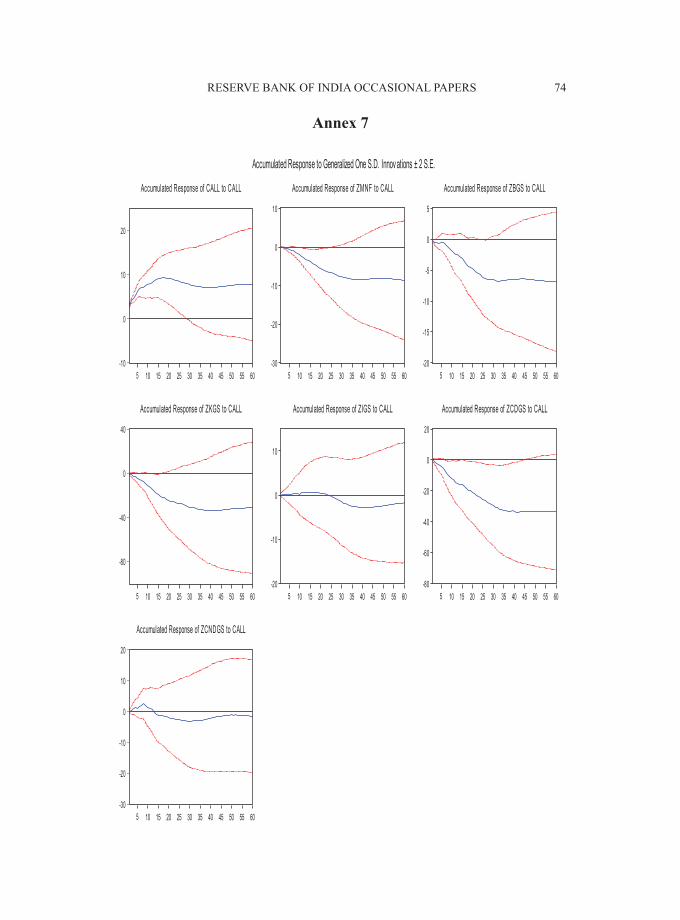
IV.2.3 Model with Core (Manufacturing) Inflation An alternative perspective to account for supply shocks entails a model with core inflation without the presence of exogenous supply shocks. Thus, we experimented with the VAR model (Model 4) with manufacturing price inflation as endogenous variable rather than aggregate price inflation as in the Model 3. The impulse response analysis arising from Model 4 is provided in Annex 7 and in Table 5. Here again the common finding was that the impact of tight money policy shock on output growth of capital goods and consumer durables in Model 4 turned out to be higher than Model 3. On other hand, the impact was more or less similar for basic goods and intermediate goods but consumer non-durables showed a lower response in Model 4 than Model 3.
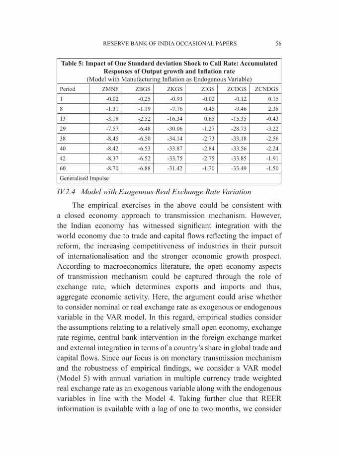
RESERVE BANK OF INDIA OCCASIONAL PAPERS 56
Table 5: Impact of One Standard deviation Shock to Call Rate: Accumulated Responses of Output growth and Inflation rate
(Model with Manufacturing Inflation as Endogenous Variable)Period ZMNF ZBGS ZKGS ZIGS ZCDGS ZCNDGS
1 -0.02 -0.25 -0.93 -0.02 -0.12 0.15
8 -1.31 -1.19 -7.76 0.45 -9.46 2.38
13 -3.18 -2.52 -16.34 0.65 -15.35 -0.43
29 -7.57 -6.48 -30.06 -1.27 -28.73 -3.22
38 -8.45 -6.50 -34.14 -2.73 -33.18 -2.56
40 -8.42 -6.53 -33.87 -2.84 -33.56 -2.24
42 -8.37 -6.52 -33.75 -2.75 -33.85 -1.91
60 -8.70 -6.88 -31.42 -1.70 -33.49 -1.50
Generalised Impulse
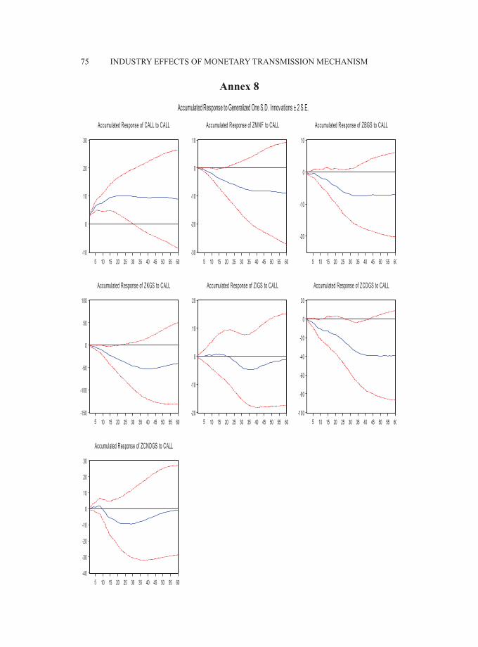
IV.2.4 Model with Exogenous Real Exchange Rate Variation
The empirical exercises in the above could be consistent with a closed economy approach to transmission mechanism. However, the Indian economy has witnessed significant integration with the world economy due to trade and capital flows reflecting the impact of reform, the increasing competitiveness of industries in their pursuit of internationalisation and the stronger economic growth prospect. According to macroeconomics literature, the open economy aspects of transmission mechanism could be captured through the role of exchange rate, which determines exports and imports and thus, aggregate economic activity. Here, the argument could arise whether to consider nominal or real exchange rate as exogenous or endogenous variable in the VAR model. In this regard, empirical studies consider the assumptions relating to a relatively small open economy, exchange rate regime, central bank intervention in the foreign exchange market and external integration in terms of a country’s share in global trade and capital flows. Since our focus is on monetary transmission mechanism and the robustness of empirical findings, we consider a VAR model (Model 5) with annual variation in multiple currency trade weighted real exchange rate as an exogenous variable along with the endogenous variables in line with the Model 4. Taking further clue that REER information is available with a lag of one to two months, we consider

INDuSTRy EFFECTS OF MONETARy TRANSMISSION MECHANISM57
one-month lag of year-on-year variation in the real exchange rate. The impulse responses arising from the Model 5 are shown in Annex 8 and Table 6. The findings from the Model 5 are notable when compared with Model 4. Though with the presence of real exchange rate variation, all sectors witnesses a strengthening of monetary impact, capital goods, intermediate goods and consumer non-durables show a significantly higher impact of tight policy in Model 5 than in Model 4.
Table 6: Impact of One Standard deviation Shock to Call Rate: Accumulated Responses of Output growth and Inflation rate
(Model with Exogenous Real Exchange rate variation)Period ZMNF ZBGS ZKGS ZIGS ZCDGS ZCNDGS
1 -0.02 -0.24 -0.95 -0.02 -0.10 0.11
8 -1.31 -1.10 -8.20 0.48 -8.94 1.55
12 -2.74 -2.20 -16.52 0.64 -12.41 -2.80
24 -5.80 -5.67 -37.23 -1.19 -21.23 -9.25
29 -6.87 -6.81 -44.23 -3.32 -28.30 -9.40
35 -7.88 -7.44 -50.57 -4.77 -35.81 -8.05
39 -8.17 -7.34 -52.56 -4.47 -37.86 -6.70
51 -8.36 -7.20 -47.01 -1.92 -39.47 -2.33
60 -8.99 -7.04 -40.30 -1.07 -38.77 -0.85
Generalised Impulse
IV.2.5 Impact of the Global Crisis
A viewpoint may arise that last four to five years could be construed as a special situation attributable to the global crisis period, necessitating rapid policy response to tackle the adverse conditions. In this context, we evaluated a VAR model (Model 3) with sample period April 1993 to March 2008, excluding the global crisis period. The impulse responses of the use-based industries to tight monetary policy shock are shown in Annex 9 and Table 7. It was evident that the crisis did not affect the underlying nature of transmission mechanism in terms of maximum impact of tight monetary policy shock on the output growth of capital goods and consumer durables. However, the magnitude of impact showed a softening during the crisis. Also, there was some evidence on the faster pace of transmission mechanism in terms of time period for the maximum impact across the sectors.

RESERVE BANK OF INDIA OCCASIONAL PAPERS 58
IV.2.6 Variance Decomposition Analysis
The forecast error variance decomposition showed the findings more or less similar to the impulse response analysis, albeit with some marginal difference. Illustratively, Table 8 provides of the Forecast Error Variance Decomposition (FEVD) analysis for the Model 4. The impact of call money rate shock in explaining total variation of output growth in the medium term (between 12-36 months) was highest for consumer durables, followed by basic goods, capital goods, consumer non-durables and intermediate goods. This finding also extended to other models. A notable finding here was that the inter-industry interaction, comprising own and other sectors’ contributions, accounting for more than three-fourth of total variation of output growth for the use-based industries. Illustratively, over 36 months, own lags reflecting the persistence of the sector accounted for 30 per cent and the lags of other sectors accounted for 58 per cent of total variation in the output growth of capital goods sector.
Table 7: Global Crisis and the Impact of One Standard deviation Shock to Call Rate: Accumulated Responses of
Output growth and Inflation ratePeriod with the Global Crisis Period without Global Crisis
Model 1 Model 2 Model 3 Model 4 Model 1 Model 2 Model 3 Model 4
Basic Goods -9.0 (33)
-7.1 (33)
-6.9 (60)
-7.4 (35)
-10.3 (33)
-9.1 (26)
-7.4 (41)
-9.1 (41)
Capital Goods
-30.4 (38)
-18.6 (24)
-34.1 (38)
-52.6 (39)
-62.0 (60)
-26.6 (60)
-37.6 (60)
-61.5 (60)
Intermediate goods
-4.8 (40)
-2.9 (40)
-2.8 (40)
-4.8 (35)
-12.8 (44)
-7.9 (34)
-8.8 (40)
-12.0 (42)
Consumer durables
-36.1 (41)
-28.2 (37)
-33.9 (42)
-39.5 (51)
-58.1 (60)
-27.5 (33)
-35.3 (60)
-47.3 (47)
Consumer non-durables
-4.5 (31)
-6.2 (60)
-3.2 (29)
-9.4 (29)
-13.4 (60)
-9.3 (29)
-9.6 (60)
-16.0 (60)
Figures indicate maximum impact in terms of cumulative impulse response to one standard deviation shock to call money rate. Figures in bracket indicate the period taken to reach maximum impact.

INDuSTRy EFFECTS OF MONETARy TRANSMISSION MECHANISM59
Table 8: Generalised Forecast Error Variance Decomposition Analysis
Horizon CALL ZINF ZBGS ZKGS ZIGS ZCDGS ZCNDGS0 0.05 0.00 1.00 0.03 0.06 0.06 0.006 0.09 0.01 0.80 0.03 0.18 0.07 0.05
12 0.15 0.02 0.69 0.03 0.15 0.08 0.0924 0.18 0.10 0.49 0.03 0.11 0.13 0.1036 0.18 0.10 0.45 0.04 0.11 0.13 0.1148 0.17 0.10 0.44 0.04 0.11 0.14 0.1160 0.17 0.10 0.44 0.04 0.11 0.14 0.11
Horizon CALL ZINF ZBGS ZKGS ZIGS ZCDGS ZCNDGS0 0.01 0.00 0.03 1.00 0.02 0.03 0.006 0.07 0.06 0.13 0.71 0.13 0.12 0.04
12 0.12 0.14 0.11 0.47 0.12 0.14 0.1324 0.12 0.15 0.09 0.33 0.09 0.14 0.2236 0.12 0.15 0.09 0.31 0.09 0.15 0.2348 0.11 0.15 0.10 0.30 0.10 0.15 0.2260 0.11 0.15 0.11 0.30 0.10 0.15 0.21
Horizon CALL ZINF ZBGS ZKGS ZIGS ZCDGS ZCNDGS0 0.00 0.00 0.06 0.02 1.00 0.13 0.006 0.01 0.02 0.09 0.04 0.92 0.09 0.02
12 0.01 0.02 0.10 0.04 0.86 0.09 0.0424 0.01 0.08 0.09 0.07 0.71 0.15 0.0636 0.03 0.09 0.10 0.07 0.66 0.14 0.0748 0.03 0.09 0.11 0.07 0.62 0.13 0.0960 0.03 0.09 0.11 0.07 0.61 0.13 0.09
Horizon CALL ZINF ZBGS ZKGS ZIGS ZCDGS ZCNDGS0 0.00 0.00 0.06 0.03 0.13 1.00 0.006 0.10 0.02 0.08 0.04 0.25 0.77 0.03
12 0.16 0.03 0.13 0.06 0.24 0.65 0.0424 0.18 0.06 0.12 0.05 0.22 0.58 0.0536 0.20 0.06 0.12 0.05 0.21 0.55 0.0548 0.19 0.06 0.13 0.05 0.21 0.54 0.0560 0.19 0.06 0.13 0.05 0.21 0.53 0.05
Horizon CALL ZINF ZBGS ZKGS ZIGS ZCDGS ZCNDGS0 0.00 0.00 0.00 0.00 0.00 0.00 1.006 0.03 0.03 0.03 0.02 0.03 0.03 0.85
12 0.07 0.05 0.06 0.02 0.05 0.04 0.7224 0.08 0.10 0.07 0.05 0.06 0.08 0.5836 0.08 0.10 0.07 0.05 0.06 0.10 0.5748 0.08 0.10 0.07 0.05 0.07 0.10 0.5660 0.08 0.10 0.07 0.05 0.07 0.10 0.55
RESERVE BANK OF INDIA OCCASIONAL PAPERS 60
Section V
Conclusion
In this study, we examined how monetary policy shock impinges on the output growth of five use-based industries such as basic goods, capital goods, intermediate goods, consumer durables, and consumer non-durable goods. The empirical findings from the VAR model with alternative combinations of variables brought to the fore a common perspective. Monetary policy could affect capital goods and consumer durables more than other three used-based industries. In some cases, basic goods also showed a response similar to durables and capital goods. Intermediate goods and consumer non-durables showed moderate response to policy shock, and the latter was also associated with a lag in transmission effect. The supply side factors affecting inflation through oil and food prices could play a role in determining the output cost of disinflation. Empirical findings suggested that without supply shocks, the impulse response of output and inflation to monetary policy could be overestimated. The industry effects of monetary transmission mechanism could also be different for an open economy with exogenous fluctuation in real exchange rate. These findings provide insights about how monetary policy affects consumption and investment demands and thereby, the economic growth and inflation. It is expected that these findings could find useful for policy analysis in the Indian context. For further research, policy analysis would benefit from studies focused on disaggregate approach to transmission mechanism based on corporate balance sheets across different industries and sectors.
References
Ahmed, S. (1987). “Wage Stickiness and the Non-Neutrality of Money: A Cross-Industry Analysis.” Journal of Monetary Economics, 20.
Ahmed, H. and S.M. Miller (1997). “Monetary and Exchange Rate Policy in Multisectoral Economies.” Journal of Economics and Business, 49.
Angeloni, I., A. Kashyap and B. Mojon (2003). Monetary Policy Transmission in the Euro Area. Cambridge university Press.

INDuSTRy EFFECTS OF MONETARy TRANSMISSION MECHANISM61
Ball, Laurence and David Romer (1990). “Real Rigidities and the Non-Neutrality of Money.” Review of Economic Studies, 57.
Barro, R.J. (1977). “unanticipated Money Growth and unemployment in the united States.” American Economic Review, 67(2).
———. (1981). “unanticipated Money, Output, and the Price Level in the united States.” in R. Barro (ed.), Money, Expectations and Business Cycles. New york: Academic Press.
Benito, A. (2002). “Financial pressure, monetary policy effects and inventory adjustment by uK and Spanish firms.” BANCO DE ESPAÑA/DOCUMENTO DE TRABAJO N.0223
Bernanke, B. and M. Gertler (1995). “Inside the Black Box: The Credit Channel of Monetary Policy Transmission.” Journal of Economic Perspectives, 9.
Bernanke, B.S. and A.S. Blinder (1988). “Credit, Money and Aggregate Demand.” American Economic Review Papers and Proceedings, 78.
Bernanke, Ben S. and Alan S. Blinder (1992). “The Federal Funds Rate and the Channels of Monetary Transmission.” American Economic Review, 82(4).
Bernanke, B.S. and M. Gertler (1995). “Inside the Black Box: The Credit Channel of Monetary Policy Transmission.” Journal of Economic Perspectives, 9.
Berument, H., N.B. Ceylan and E.M. yucel (2004). “The Differential Sectoral Effects of Policy Shocks: Evidence from Turkey.” Working Paper No. 0703, Bilkent University, Department of Economics.
Berument, H., N. Konac and O. Senay (2007). “Openness and the Effectiveness of Monetary Policy: A Cross-country Analysis.” International Economic Journal, 21(4).
Blinder, A. and Mankiw, N.G. Jan. (1984). “Aggregation and Stabilization Policy in a Multicontract Economy.” Journal of Monetary Economics, 13(1).
Dale, S. and A.G. Haldane (1995). “Interest Rates and the Channels of Monetary Transmission: Some Sectoral Estimates.” European Economic Review, 39.

RESERVE BANK OF INDIA OCCASIONAL PAPERS 62
David, I.C., J.J. Durand and N. Payelle (2000). “The Heterogeneous Effects of Monetary Policy in the Euro Area: A Sectoral Approach.” France: university of Rennes.
Dedola, L. and F. Lippi (2000). “The Monetary Transmission Mechanism: Evidence from the Industries of five OECD Countries.” Temi di discussione 389, Bank of Italy.
Dhal, S. (2012). “A Disaggregated Monetary Transmission Mechanism: Evidence from Dispersion of bank Credit to Indian States.” in the Regional Economy of India: Growth and Finance, edited by Deepak Mohanty, Academic Foundation and RBI.
Drake, L. and Adrian R. Fleissig (2010). “Substitution between monetary assets and consumer goods: New evidence on the monetary transmission mechanism.” Journal of Banking and Finance, 34.
Duca, J.V. and D.D. VanHoose (1990). “Optimal Monetary Policy in a Multisectoral Economy with an Economy-wide Money Market.” Journal of Economics and Business, 42(4).
Edwards, S. (1989a). “Openness, Outward Orientation, Trade Liberalization and Economic Performance in Developing Countries.” NBER Working Paper No. 2908.
———. (1989b). “Exchange Controls, Devaluations and Real Exchange Rates: the Latin American Experience.” Economic Development and Cultural Change, 37(3).
Ehrmann, M. and M. Ellison (2002). “The Changing Response of uS Industry to Monetary Policy.” CEPR Papers. uK.
Enders, W. and B. Falk (1984). “A Microeconomic Test of Money Neutrality.” The Review of Economics and Statistics, 66(4).
Erceg, C. and A. Levin (2002). “Optimal Monetary Policy with Durable and Non-Durable Goods.” ECB Working Paper No. 179.
Farès, J. and S. Gabriel (2001). “The Monetary Transmission Mechanism at the Sectoral Level.” Bank of Canada Working Paper 2001-27.

INDuSTRy EFFECTS OF MONETARy TRANSMISSION MECHANISM63
Fiorentini, R. and R. Tamborini (2001). “The Monetary Transmission Mechanism in Italy: the Credit Channel and a Missing Ring.” Giornale degli Economisti e Annali di Economia, 60(1).
Franco, Francesco and Thomas Philippon (2004). “Firms and Aggregate Dynamics.” Manuscript. New york university.
Gaiotti, E.G. and A. Generale (2001). “Does Monetary Policy have Asymmetric Effects? A Look at the Investment Decisions of Italian Firms.” European Central Bank Working Paper Series 110.
Ganley, J. and C. Salmon (1997). “The Industrial Impact of Monetary Policy Transmission: the Case of Italy.” Temi di discussione, 430, Bank of Italy.
Gauger, J. (1988). “Disaggregate Level Evidence on Monetary Neutrality.” The Review of Economics and Statistics, 70(4).
Gauger, J. and W. Enders (1989). “Money Neutrality at Aggregate and Sectoral Levels.” Southern. Economic Journal, 55.
Gerlach, S. and F. Smets (1995). “The Monetary Transmission Mechanism: Evidence from the G-7 Countries.” CEPR Discussion Paper 1219.
Gertler, M. and S. Gilchrist (1993). “The Role of Credit Market Imperfections in the Monetary Transmission Mechanism: Argument and Review.” Scandinavian Journal of Economics 95(1).
Gertler, M. and S. Gilchrist (1994). “Monetary Policy, Business Cycles and the Behavior of Small Manufacturing Firms.” Quarterly Journal of Economics, 109(2).
Greenspan, A. (2001). “Testimony of Chairman Alan Greenspan- Federal Reserve Board’s semi-annual monetary policy report to the Congress Before the Committee on Financial Services”, u.S. House of Representatives July 18, 2001.
Guiso, L., A. Kashyap, F. Panetta and D. Terlizzese (1999). “Will a Common European Monetary Policy have Asymmetric Effects?” Economic Perspectives, Federal Reserve Bank of Chicago.

RESERVE BANK OF INDIA OCCASIONAL PAPERS 64
Hayo, B. and B. uhlenbrock (1999). “Industry Effects of Monetary Policy in Germany.” Center for European Integration Studies Working Paper No. B 14.
Jung, y and T. yun (2005). “Monetary policy, inventory dynamics and price setting behavior.” Federal Reserve Bank Sanfransisco Working Paper 2006-02.
Kandil, M. (1991). “Variations in the Response of Real Output to Aggregate Demand Shocks: A Cross Industry Analysis.” Review of Economics and Statistics, 73.
Kashyap, A.K. and J. Stein (1994). “Monetary Policy and Bank Lending.” in N.G. Mankiew (ed.), Monetary Policy. Chicago: university of Chicago Press.
————. (2000). “What do a Million Observations on Banks say about the Transmission of Monetary Policy?” American Economic Review, 90(3).
Kashyap, A.K. and J.C. Stein (1995). “The Impact of Monetary Policy on Bank Balance Sheets.” Carnegie-Rochester Conference Series on Public Policy, 42.
Kashyap, A.K., J. Stein and D.W. Wilcox (1993). “Monetary Policy and Credit Conditions: Evidence from the Composition of External Finance.” American Economic Review, 83(1).
Kim, S. (1999). “Do Monetary Policy Shocks Matter in the G-7 Countries? using Common Identifying Assumptions about Monetary Policy Across Countries.” Journal of International Economics, 48(2).
Kretzmer, P.E. (1989). “The Cross-Industry Effects of unanticipated Money in an Equilibrium Business Cycle Model.” Journal of Monetary Economics, 23.
Lastrapes, William D. (2006). “Inflation and the Distribution of Relative Prices: The Role of Productivity and Money Supply Shocks.” Journal of Money, Credit and Banking, 38(8).
Linde, J. (2003). “Comment on the Output Composition Puzzle: A Difference in the Monetary Transmission Mechanism in the Euro Area and u.S.” Journal of Money, Credit, and Banking, 35.

INDuSTRy EFFECTS OF MONETARy TRANSMISSION MECHANISM65
Llaudes, R. (2007). “Monetary Policy Shocks in a Two-Sector Open Economy: An Empirical Study.” European Central Bank Working Paper Series No 799.
Loo, C.M. and W.D. Lastrapes (1998). “Identifying the Effects of Money Supply Shocks on Industry-Level Output.” Journal of Macroeconomics, 20(3).
Lutkepohl, H. (1990). “Asymptotic Distributions of Impulse Response Functions and Forecast Error Variance Decompositions of Vector Autoregressive Models.” Review of Economics and Statistics,72(1)
Lütkepohl, H. and D. S. Poskitt (1991). “Estimating Orthogonal Impulse Responses via Vector Autoregressive Models.” Econometric Theory, 7(4).
Lütkepohl, H. R. BrÄuggemann and P. Saikkonen (2006). “Residual Autocorrelation Testing for Vector Error Correction Models.” Journal of Econometrics, 134.
Lütkepohl, H (2006). Vector Autoregressive Models, in T.C. Mills & K. Patterson (Eds.), Palgrave Handbook of Econometrics, Volume 1, Econometric Theory, Houndmills: Palgrave Macmillan, 2006, 477-510.
Mishkin, F. (1976). “Illiquidity, Consumer durable expenditure and Monetary Policy.” American Economic Review, 66(4)
Pesaran, H. Hashem, and y. Shin (1998). “Generalized impulse response analysis in linear multivariate models.” Economics Letters, 58: 17–29
Peersman, G. and F. Smets (2001). “The Monetary Transmission Mechanism in the Euro Area: More Evidence from VAR Analysis.” European Central Bank Working Paper No.91.
————. (2002). “The Industry Effects of Monetary Policy in the Euro Area.” European Central Bank, Working Paper No.165.
————. (2005). “The Industry Effects of Monetary Policy in Euro Area.” Economic Journal, 115(503): 319-342
RESERVE BANK OF INDIA OCCASIONAL PAPERS 66
Ramaswamy, R. and T. Sloek (1997). “The Real Effects of Monetary Policy in the European union: What Are the Differences.” IMF Working Paper No.160. Washington: IMF.
Shelley, G.L. and F. H. Wallace (1998). “Tests of the Money-Output Relation using Disaggregated Data.” The Quarterly Review of Economics and Finance, 38(4).
Stiglitz, J. and A. Weiss (1981). “Credit Rationing in Markets with Imperfect Information.” American Economic Review, 71: 393-410.
Taylor, L.L. and M.K. yucel (1996). “The Policy Sensitivity of Industries and Regions.” Working Paper No.12. Federal Reserve Bank of Dallas.
Waller, C.J. (1992). “The Choice of Conservative Central Banker in a Multisectoral Economy.” American Economic Review, 82(4).

INDuSTRy EFFECTS OF MONETARy TRANSMISSION MECHANISM67
Annex 1: Principal Component Analysis (PCA) of Broad GDP Components:
Agriculture, Industry and Services Sectors
Ordinary Correlation Based PCA
Eigen values: (Sum = 3, Average = 1)Number Value Difference Proportion Cumulative
Value1 1.444435 0.465440 0.4815 1.4444352 0.978995 0.402424 0.3263 2.4234303 0.576570 --- 0.1922 3.000000
Eigenvectors (loadings): Variable PC 1 PC 2 PC 3 XGAGS 0.283025 0.937788 0.201121XGINDS 0.658422 -0.342452 0.670229XGSRVS 0.697408 -0.057269 -0.714383Ordinary correlations:
XGAGS XGINDS XGSRVSXGAGS 1.000000XGINDS 0.032489 1.000000XGSRVS 0.149690 0.406406 1.000000
Ordinary (uncentered) Correlation Based PCA
Eigen values: (Sum = 3, Average = 1)Number Value Difference Proportion Cumulative
ValueCumulative Proportion
1 2.256865 1.601170 0.7523 2.256865 0.75232 0.655696 0.568257 0.2186 2.912561 0.97093 0.087439 --- 0.0291 3.000000 1.0000
Eigenvectors (loadings): Variable PC 1 PC 2 PC 3 XGAGS 0.464988 0.883436 0.057677XGINDS 0.620079 -0.371487 0.691013XGSRVS 0.631893 -0.285548 -0.720537

RESERVE BANK OF INDIA OCCASIONAL PAPERS 68
Ordinary (uncentered) correlations:XGAGS XGINDS XGSRVS
XGAGS 1.000000XGINDS 0.439016 1.000000XGSRVS 0.494075 0.910311 1.000000

INDuSTRy EFFECTS OF MONETARy TRANSMISSION MECHANISM69
Annex 2: Major Product Items in Use-based IndustriesBasic goods Capital goods Intermediate goods Consumer durables Consumer
non-durabelsproducts weight products weight products weight products weight products weight
Minerals 141.6 Com-mercial Vehicles
19.3 Cotton yarn
15.1 Passenger Cars
19.7 Antibiotics 23.8
Electricity 103.2 Boilers 4.0 LPG 11.2 Gems & Jewellery
17.7 Apparels 20.3
Cement 24.1 Tractors 3.8 Non-cot-ton yarn
7.1 Motor Cycles
9.5 sugar 15.2
Diesel 21.1 Three-Wheelers
3.3 Fasteners 5.7 Colour TV 3.8 Newspa-pers
10.1
H R Coils 13.0 Refractory Bricks
3.2 Petrol 5.6 Glazed /Ceramic Tiles
3.6 grey cloth 9.1
Plates 12.5 Grinding Wheels
2.9 Synthetic yarn
5.5 Air Condi-tioner
2.9 Cigarettes 8.7
sponge iron
10.0 Engines 2.9 Steel Structures
5.5 Woollen Carpets
2.6 Cotton cloth
8.0
Bars & Rods
9.8 Plastic Machinery
2.6 Naphtha 5.4 Wood Furniture
2.4 Leather Garments
7.5
Carbon steel
7.8 Trans-formers
2.4 Block Board
5.1 Tyre, Truck/Bus
2.4 Rice 6.6
urea 6.4 Computers 2.3 Purified acid
4.2 Telephone Instru-ments Including Mobile
2.2 Tea 6.5
Stainless/ alloy steel
6.4 Earth Moving Machinery
2.3 Furnace Oil
3.9 Scooter and Mo-peds
2.1 Pens of All Kind
5.9
Ferro manga-nese
6.4 Switch-gears
2.2 Bearings (Ball/Roller)
3.4 Pressure Cooker
2.1 Milk, Skimmed, Pasteurised
5.7
CR Sheets 5.6 Conductor, Alumin-ium
2.0 Polypro-pylene
3.0 Tyre, Car/Cab
2.0 Razor/Safety Blades
5.3
Copper and Prod-ucts
5.5 Air & Gas Compres-sors
1.9 Industrial Alcohol
2.6 PVC Pipes and Tubes
1.9 Biri 5.1
Stampings & Forg-ings
4.9 Textile Machinery
1.7 Glass Bottles
2.6 Marble Tiles/Slabs
1.2 Non-cotton cloth
3.9
sub-total 378.2 sub-total 56.8 sub-total 85.9 sub-total 76.2 sub-total 141.7
All 456.8 All 88.3 All 156.9 All 84.6 All 213.5
RESERVE BANK OF INDIA OCCASIONAL PAPERS 70
Annex 3
-25
-20
-15
-10
-5
0
5
5 10 15 20 25 30 35 40 45 50 55 60
Accumulated Response of ZQS to CALL
-20
-15
-10
-5
0
5
5 10 15 20 25 30 35 40 45 50 55 60
Accumulated Response of ZINF to CALL
-5
0
5
10
15
5 10 15 20 25 30 35 40 45 50 55 60
Accumulated Response of CALL to CALL
Accumulated Response to Generalized One S.D. Innovations ± 2 S.E.
INDuSTRy EFFECTS OF MONETARy TRANSMISSION MECHANISM71
Annex 4

RESERVE BANK OF INDIA OCCASIONAL PAPERS 72
Annex 5

INDuSTRy EFFECTS OF MONETARy TRANSMISSION MECHANISM73
Annex 6
-10
-5
0
5
10
15
20
5 10 15 20 25 30 35 40 45 50 55 60
Accumulated Response of CALL to CALL
-20
-10
0
10
5 10 15 20 25 30 35 40 45 50 55 60
Accumulated Response of ZINF to CALL
-20
-16
-12
-8
-4
0
4
5 10 15 20 25 30 35 40 45 50 55 60
Accumulated Response of ZBGS to CALL
-80
-40
0
40
5 10 15 20 25 30 35 40 45 50 55 60
Accumulated Response of ZKGS to CALL
-20
-10
0
10
20
5 10 15 20 25 30 35 40 45 50 55 60
Accumulated Response of ZIGS to CALL
-80
-60
-40
-20
0
20
5 10 15 20 25 30 35 40 45 50 55 60
Accumulated Response of ZCDGS to CALL
-30
-20
-10
0
10
20
5 10 15 20 25 30 35 40 45 50 55 60
Accumulated Response of ZCNDGS to CALL
Accumulated Response to Generalized One S.D. Innovations ± 2 S.E.
RESERVE BANK OF INDIA OCCASIONAL PAPERS 74
Annex 7
INDuSTRy EFFECTS OF MONETARy TRANSMISSION MECHANISM75
Annex 8

RESERVE BANK OF INDIA OCCASIONAL PAPERS 76
Annex 9a

INDuSTRy EFFECTS OF MONETARy TRANSMISSION MECHANISM77
Annex 9b

RESERVE BANK OF INDIA OCCASIONAL PAPERS 78
Annex 9c

INDuSTRy EFFECTS OF MONETARy TRANSMISSION MECHANISM79
Annex 9d