Industrial structure and child labour. Working Paper Seri ... · local area employment in Brazil...

1.

Industrial structure and child labour.Evidence from Brazil

M. ManacordaF. C. Rosati

February 2008

Und

erst

andi

ng C

hild

ren’

s Wor

k Pr

ojec

t Wor

king

Pap

er S

erie

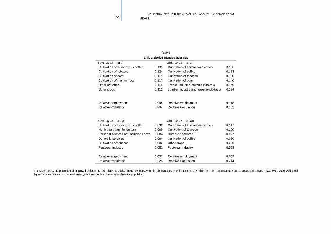
s, Fe

brua

ry 2

008

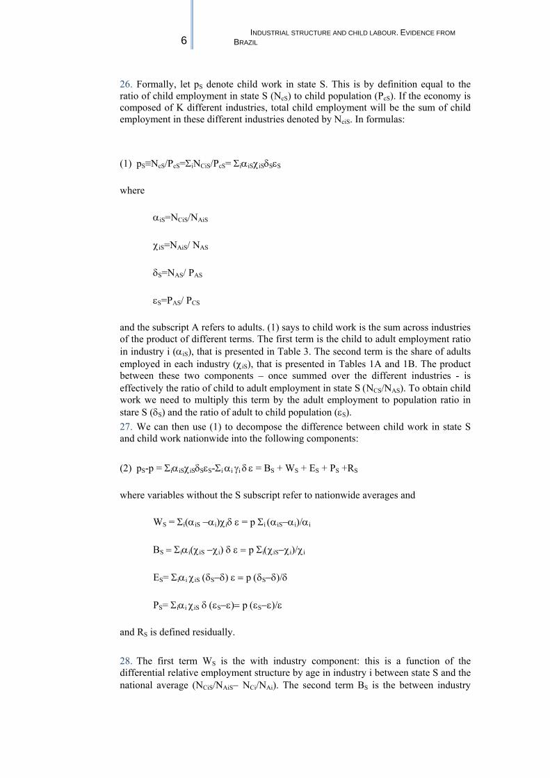
Industrial structure and child labour. Evidence from Brazil

M. Manacorda*

F. C. Rosati**

Working Paper February 2008

Understanding Children’s Work (UCW) Project

University of Rome “Tor Vergata” Faculty of Economics

V. Columbia 2 00133 Rome Tor Vergata

Tel: +39 06.7259.5618 Fax: +39 06.2020.687

Email: [email protected]

As part of broader efforts toward durable solutions to child labor, the International Labour Organization (ILO), the United Nations Children’s Fund (UNICEF), and the World Bank initiated the interagency Understanding Children’s Work (UCW) project in December 2000. The project is guided by the Oslo Agenda for Action, which laid out the priorities for the international community in the fight against child labor. Through a variety of data collection, research, and assessment activities, the UCW project is broadly directed toward improving understanding of child labor, its causes and effects, how it can be measured, and effective policies for addressing it. For further information, see the project website at www.ucw-project.org.

This paper is part of the research carried out within UCW (Understanding Children's Work), a joint ILO, World Bank and UNICEF project. The views expressed here are those of the authors' and should not be attributed to the ILO, the World Bank, UNICEF or any of these agencies’ member countries.

*Department of Economics, QMUL Centre for Economic Performance, LSE and CEPR ** UCW-Project and University of Rome “Tor Vergata”



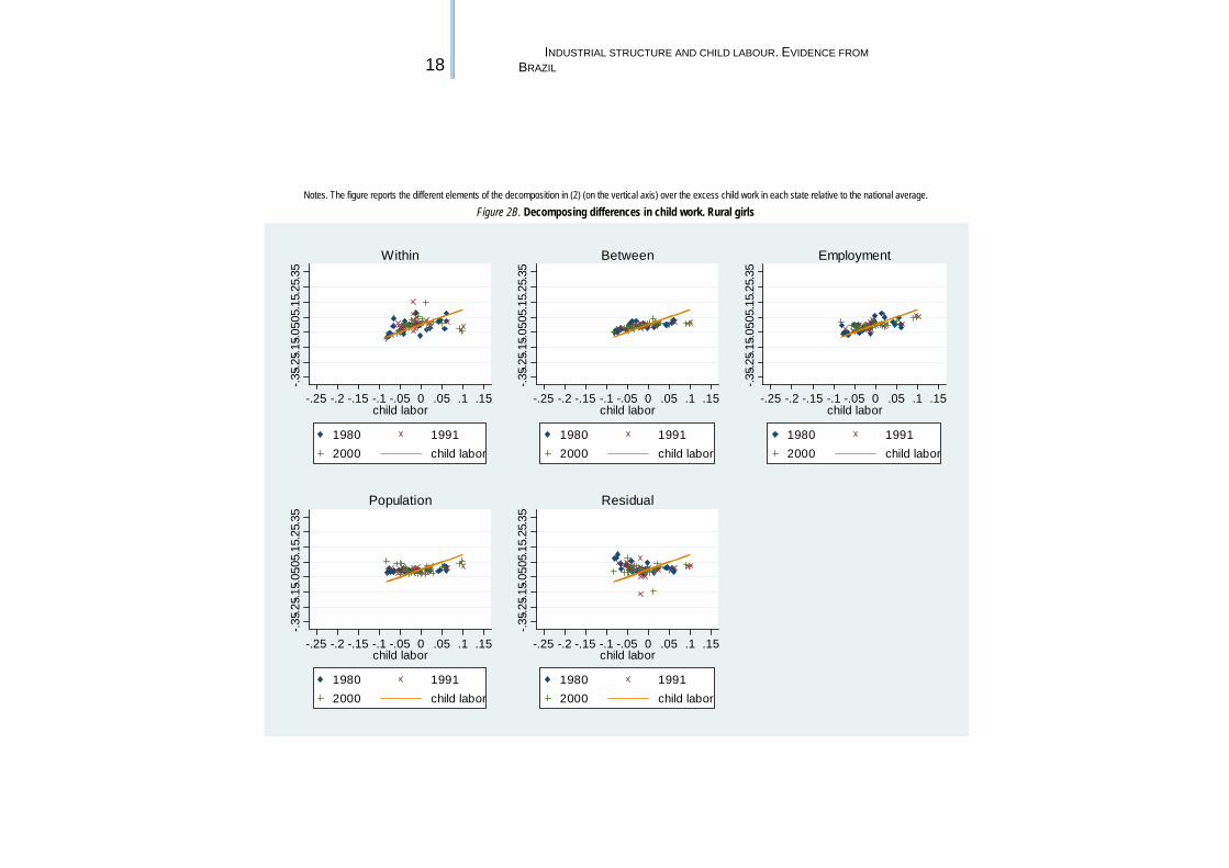
ABSTRACT

In this paper we investigate whether the differential evolution of child work across Brazilian states between 1980 and 2000 can be explained by their different patterns of specialization in industries where children have a comparative advantage. We find that the adoption of different industries mixes by different states accounts for 20% to 30% of the observed variation in child labor in rural areas while we find little or no effect in urban areas.

We are grateful to Cristina Valdivia for excellent research assistance.



CONTENTS

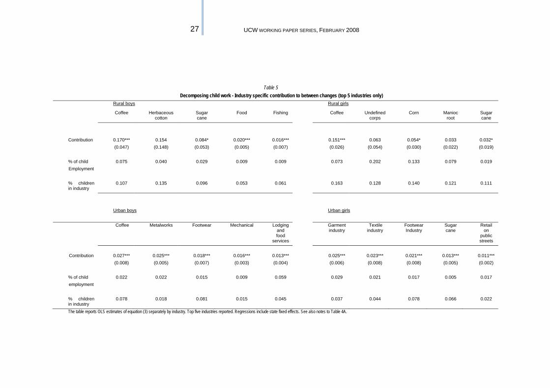
Introduction ............................................................................................................................... 1 1. Data and descriptive analysis ......................................................................................... 2 2. Methodology .................................................................................................................. 5 3. Empirical results ............................................................................................................ 8

3.1 Results by industry ................................................................................................. 10 4. Conclusions .................................................................................................................. 11 References ............................................................................................................................... 13 Data Appendix ......................................................................................................................... 15

1 UCW WORKING PAPER SERIES, FEBRUARY 2008

INTRODUCTION 1. Children work in a variety of economic sectors, but little is known about the role that the characteristics of production in each sector play in determining the extent of child work. If there are sectors that demand a disproportionate share of children in their workforce, then interventions targeting specific sectors of the economy could be warranted. On the other hand, if the presence of children in the workforce is mainly determined by supply, then policies should be targeted to vulnerable household. It is of course very difficult to answer this question: ideally this would require estimating a full labor market sectoral equilibrium model, an objective made difficult both by the lack of data and by the technical difficulties in identifying the relevant parameters. 2. In this paper we begin to address this issue by using micro data from the Brazilian population Census between 1980 and 2000 to study the role of the sectoral distribution of employment in accounting for the incidence of child labor. 3. A large amount of literature has been produced on the phenomenon of child work. We have solid evidence that improvements in living standards - with the ensuing fall in the supply of child work - and the generalized rise in the demand for skills - that reduces the demand for child work - are both responsible for the secular fall children’s employment that is typically associated to economic development (for all, see Edmonds, 2007, and references therein). Economic progress, with the associated increase in the demand for skills, also reduces the incentives to engage in work at an early age, since the opportunity cost of dropping out of school increases over time. The same variables are also potentially able to explain cross-sectional differences in the incidence of child work across countries at different stages of development. 4. As also noted by Edmonds (2007), much of the emphasis in the literature is on the labor supply determinants of child work. The increasing availability of micro data from household surveys for many developing countries has allowed researchers to investigate the children’s decisions in the context of their household supply, link work and schooling decisions, investigate the role of credit constraints and poverty, and understand the role that household production among rural households plays in shaping child work (for a detailed review see Edmonds, 2007 and for a discussion of the theory underpinning child work decisions see Cigno and Rosati, 2005). 5. Less attention has been paid to the demand side. Some studies analyze temporary changes in local labor demand and/or local economic conditions. Guarcello, Lyon and Rosati (2005) for example illustrate the importance of local labor markets condition in determining permanence in school and participation in the labor market in Ethiopia. Similarly Parikh and Sadoulet (2005) find a positive association between local area employment in Brazil while Manacorda and Rosati (2007) present a more nuanced picture, showing that child work responses in Brazil vary substantially according to gender, age and household wealth and location. Again on Brazil, Kruger (2007) shows that an increase in the value of coffee production induces a rise in child work among children (of parents with low or intermediate levels of education). 6. Other work has been trying to establish whether children enjoy a comparative advantage with respect to adults in certain productions and whether this in turn in responsible for the incidence of child work. It is probably not incorrect to say that the existing research in this area is scarce and the findings heterogeneous. Goldin and Sokoloff (1982) for example argue that the rapid process of industrialization in the American Northeast during the first half of the nineteenth century lead a fast rise in the demand for child work due to the expansion of the manufacturing sector that was typically child work intensive. Edmonds (2003) finds that little evidence of an

2 INDUSTRIAL STRUCTURE AND CHILD LABOUR. EVIDENCE FROM

BRAZIL

association between children’s involvement in economic activity and variation in types of industries (over time or between locations), including manufacturing, in contemporary Vietnam. Similarly, while work by Sloutsky and Fisher (2004) and Koutstaal and Schacter (1997) seems to imply that children might have an advantage at work that requires patterns memorization, evidence in support of the “nimble fingers” hypothesis is weak (Levison et al, 1998, and Edmonds, 2007). 7. In this paper we examine more closely the question of whether sector specific labor demand is responsible for the differential incidence of child work across Brazilian states and its differential change over time. Child work is widespread in Brazil. Although this has been declining especially since the mid 1990s (see for example Manacorda and Rosati, 2006), there is still no consensus on the determinants of such decline. Improvements in living standards, increasing urbanization, rising public pressure and the adoption of State and Federal policies aimed specifically at promoting school attendance and curbing child might have all played a role.2 Here we concentrate on a different channel, namely the declining weight of child intensive industries in the economy. 8. The structure of the paper is as follows. In section 1 we present the data and we analyze the sectoral employment distribution of children vis à vis adults. Section 2 lays out the methodology (borrowed by Lewis, 2004) used in section 3 to decompose the incidence of child work into its between and within industry components. Section 4 finally concludes.

1. DATA AND DESCRIPTIVE ANALYSIS 9. For the purpose of this exercise we use micro data from the IPUMS version of the Brazilian Population census (Minnesota Population Center, 2007) for the years 1980, 1991 and 2000.3 Consistently throughout the period of observation, the data provide information on labor market participation for all individuals aged 10 or above. Sample sizes are very large and increase over time, going from around 5.8 million observations in 1980 to more than 10 million observations in 2000. We define as children those aged 10 to 15. Work activity refers to the week before the census week and includes both paid and unpaid economic work. The data exclude non economic activities such as household chores. For those in work, the census ascertains the sector of activity at the three digit level. Because the classification of activities changes considerably over time (the number of sectors grows from 167 in 1980, to 169 in 1991 to 222 in 2000), we have proceeded to standardize the industrial classification. Details about this procedure and the resulting classification are contained in the appendix to the paper. Overall we end up with 105 industrial categories that are consistently defined throughout the period of observation. 10. Figure 1 provides a synthetic picture of the distribution of child work across Brazilian states and its change over time. The figure plots the proportion of working children in 2000 (on the vertical axis) over the proportion in 1980 (on the horizontal axis) by state. A solid line represents the 45 degree line. Data points below (above) the solid line are associated to a fall (rise) in child work in that state. We use sampling weights to get population estimates and we present separate results for boys and girls in rural and urban areas. 2 The evidence on the effect of Bolsa Escola on child labor however seems to suggest no effect (Cardoso and Souza, 2004). 3 IPUMS Census data for Brazil are available since 1970. The problem with the 1970 data, though, is that the classification of industries is too coarse in that year. Around 40% of children would be in fact classified in the “undefined crops” category. To avoid this problem, we only restrict to data from 1980 onwards.


11. On average the proportion of working boys in rural Brazil in 1980 was 36%. However, there is a large variation across states. States with a significantly higher incidence of child work are in the poorer Northeast (Piauí, Paraiba, Pernambuco and Ceara) and North (Rondonia and Acre) while the states in the South and Centre display typically below average levels of child labor. 12. The figure shows a generalized fall in child work among rural boys over the twenty years of observation. The nationwide proportion of children in wok falls by around 30% (to 24%). This is represented visually by the fact that all the observations lie below the 45 degree line. With few exceptions, the ranking of different states remains largely unchanged.4 13. Results for girls in rural areas are quite different. First, in 1980 girls are on average less likely to devote to economic activities and the dispersion across states is also lower. Second, one observes little or no improvement in the propensity of rural girls to work over the 20 years of observation. Child work remains in the order of 10%. Again, with the exception of few states, the ranking of different states remains virtually unchanged. 14. In urban areas, one observes a lower incidence of child work than in rural areas. Child work in 1980 is the order of 15% and 10% respectively for boys and girls. More interestingly, one observes not only a generalized fall in child work but also a clear convergence across states. The data points lie roughly on an horizontal line, especially for girls. By 2000, child work is in the order of 7% for urban boys and 4% for urban girls. 15. Because Brazil becomes increasingly urbanized over the period of observation (the share of children in urban areas grows from approximately 68% to 80% between 1980 and 2000), this also contributes to a fall in child work. Between 1980 and 1990 child work nationwide halves: it goes from 23% to 11% for boys and from 10% to 6% for girls. 16. Having ascertained that there is large variation both across states and over time in child work, Table 1A starts by presenting the distribution of employment by industry in rural areas of Brazil. Unless otherwise noted, this and the following tables pool individuals from the three censuses and present time averages of the relevant variables. The table reports the top six industries of employment for children and adults (aged 16-60). Not surprisingly, children in rural areas are largely involved in farming and livestock raising. Corn, manioc, rice and coffee, together with other (uncategorized) crops account for almost two thirds of boys’ work in rural areas. A similar picture emerges for girls, who also appear to be involved in domestic services (15%). Girls appear to be relatively less likely than boys to work in the rice cultivation and livestock raising but more likely to work in tobacco. Results for adults are reported in the middle panel. Prime age men and women in rural Brazil appear to be involved in similar activities as children. The only exception being public education that accounts for around 10% of rural women’s employment. 17. Potentially a more appropriate comparison is between children and unskilled adults, for whom figures are presented at the bottom of the table. We define as unskilled adults those with zero years of education. Effectively, in rural areas there is a clear correspondence between boys and girls employment structure and the one of uneducated adults.

4 Notice in particular that the Federal district experiences the larges fall in child labor. Indeed, the Federal district, under the impulse of governor Buarque, was the first state to ntrodcute in 1995 a sufccesful condtional cash tansfer program (Bola escola) wehose ocverage was later epxaned to the rest of the country.


BRAZIL

18. Results for children in urban areas are reported in Table 1B. Boys appear to be involved in repairs and maintenance services (8%) and construction (8%), two sectors potentially involving an apprenticeship element and so typical destination for children and teenagers. Another important proportion (around 17%) is employed in the hospitality and retail industries (including street selling), typically low productivity and low skills sectors. The top six industries account for only about a third of urban boys’ total employment. By converse, girls in urban area are strongly concentrated in specific industries. Domestic services in particular account for more than half of girls’ employment in urban Brazil. A non negligible proportion of girls are employed in the hospitality and retail sector (9%) and in the textile and garment industry (5%). The data show clearly that, differently from rural areas, adults happen to be employed in rather different industries from children. Except for construction and maintenance services, none of the top male adult industries features among the top children’s categories. For females, three categories that are prominent among young girls are also top destinations for prime age women (domestic services, lodging and food services and the garment industry). Again, as predictable, even in urban areas we find a closer correspondence between children and uneducated adults, although these two groups are still more dissimilar than in rural areas. Domestic service feature prominently as a sector of employment of urban unskilled women (40%) and the hospitality and retail sector account respectively for 7% and 10% of unskilled adult male and female employment in urban areas. 19. As a more formal analysis of the correspondence between children’s and adult’s employment structure, Table 2 reports Duncan segregation indexes based on the industry distribution. We report three values of the index: for children compared to those aged 16-24, 25-50 and 51-60. Rural boys present a segregation index relative to adult males aged 25-50 in the order of 21%, implying that around one in five children should change employment in order for their employment distribution to mirror the one of adults. Not surprisingly, the sectoral distribution of employment among children appears marginally closer to the one of youths. The segregation index with respect to those aged 16-24 is 0.17. Perhaps surprisingly, rural boys show an even stronger similarity to older males (the Duncan segregation index is 0.14). It is possible that less productive workers (i.e. the very young or the relatively old) happen to be in similar industries. Results for girls are similar, although in general there is more divergence between young girls and prime age women than what found for males. The second row of the table reports the same index relative to unskilled adults. As expected, the segregation index falls considerably. For example, it is found that around 13% of young boys in rural areas should change their sector of employment to have the same distribution as the one of prime age uneducated men. 20. Consistently with what found in Table 1B, urban children display higher segregation than rural children. The Duncan index between rural children and prime age adults is 0.32 for males and 0.44 for females. Although similar to what found in rural areas, the segregation index falls when girls are compared to unskilled women, the same is not true for boys relative to unskilled men. Here, the segregation index, if anything rises modestly. 21. One concern with these results is that children might appear to be in similar occupations to adults, especially in rural areas, due to the definition of industries adopted. In particular, if the industrial classification is too coarse one will mechanically find children and adults in similar occupations and the Duncan index will be artificially low. To check for this, in the bottom part of Table 2 we report the same index computed based on the original industrial classification in each of the different censuses. One can see that results are very similar. The Duncan index grows modestly for boys and falls modestly for girls but the basic picture remains


unchanged, with segregation indexes in the order of 0.20 to 0.40, with girls being slightly more segregated than boys compared to their adult counterparts, with urban children displaying more dissimilarity with respect to their adult counterparts than rural children, and with children being more similar to unskilled adults in their sectoral employment distribution than to the entire adult population (with the exception of urban boys). 22. Tables 1A and 1B report the probability of being in different industries conditional on age (and in employment). A separate question is what industries are more child work intensive. This is equivalent to estimating the probability of being a child conditional on being in employment among those of working age (defined as those aged 10 to 60). Table 3 reports these probabilities for the four children groups. The most child intensive industries in urban areas are cotton, tobacco, coffee and manioc root. For example, tobacco employs 1.35 boys aged 10 to 15 for each 10 men aged 16-60. This compares to an average relative employment probability of 0.98 and a relative probability of being in the population of 2.94. So while there are approximately 3 children for each 10 adults in the population, only one will be employed. A similar picture emerges for girls, although – if anything – relative employment of girls is higher than the one of boys (0.118 versus 0.098), this presumably being due to adult women being on average less likely to participate in the labor market. Child relative population and even more so child relative employment are lower in urban areas compared to rural areas. Around 2.2 children for each 10 adults live in urban areas, compared to around 3 in rural areas, and around 1 child for each 30 adults is employed, compared to a ratio of 1 to 10 in rural areas. The sectors where urban children are disproportionately more concentrated are linked to agricultural, horticultural and floricultural production. This is also true in urban areas, although obviously these are sectors that account for a relatively small shares of employment in urban areas. Interestingly, both girls and boys account for a non negligible share of employment in the footwear industry: around 1 child is employed per 12 adult employees. 23. To summarize, in rural areas, some of the industries that account for a large proportion of children’s employment also feature a relatively high share of children. These are in particular corn and manioc root. In urban areas instead, children account for a relatively large share of the workforce in sectors that account overall for a small proportion of children’s employment.

2. METHODOLOGY 24. In this section we lay out the methodology needed to ascertain how much of the incidence of child work can be attributed to the fact that children are concentrated in specific industries. We use a simple modified version of the traditional shift-share decomposition that is borrowed by Lewis (2004). Shift share (or variance) decompositions are often used to understand the determinants of changes in the employment (or wage) of specific groups (see for example Bound and Freeman, 1992 for an analysis of the employment of blacks in the USA, Card and Lewis, 2007 for an analysis of the fortunes of immigrants to the US, and Katz and Autor, 1999 for an analysis of changes in the returns to skills). 25. We exploit the cross-sectional variation across Brazilian states to decompose child work into a component due to between industry differentials, a component to within industry differentials, the effect of total employment and the effect of population size.


BRAZIL

26. Formally, let pS denote child work in state S. This is by definition equal to the ratio of child employment in state S (NcS) to child population (PcS). If the economy is composed of K different industries, total child employment will be the sum of child employment in these different industries denoted by NciS. In formulas: (1) pS≡NcS/PcS=ΣiNCiS/PcS= ΣiαiSχiSδSεS

where

αiS=NCiS/NAiS

χiS=NAiS/ NAS

δS=NAS/ PAS

εS=PAS/ PCS

and the subscript A refers to adults. (1) says to child work is the sum across industries of the product of different terms. The first term is the child to adult employment ratio in industry i (αiS), that is presented in Table 3. The second term is the share of adults employed in each industry (χiS), that is presented in Tables 1A and 1B. The product between these two components – once summed over the different industries - is effectively the ratio of child to adult employment in state S (NCS/NAS). To obtain child work we need to multiply this term by the adult employment to population ratio in stare S (δS) and the ratio of adult to child population (εS). 27. We can then use (1) to decompose the difference between child work in state S and child work nationwide into the following components: (2) pS-p = ΣiαiSχiSδSεS-Σi αi γi δ ε = BS + WS + ES + PS +RS

where variables without the S subscript refer to nationwide averages and

WS = Σi(αiS −αi)χiδ ε = p Σi (αiS−αi)/αi

ΒS = Σiαi(χiS −χi) δ ε = p Σi(χiS−χi)/χi

ES= Σiαi χiS (δS−δ) ε = p (δS−δ)/δ

PS= Σiαi χiS δ (εS−ε)= p (εS−ε)/ε

and RS is defined residually. 28. The first term WS is the with industry component: this is a function of the differential relative employment structure by age in industry i between state S and the national average (NCiS/NAiS− NCi/NAi). The second term BS is the between industry


component: this is a function of the differential adult employment across industries in state S relative to the national average (NAiS/NAS - NAi/NA). The term ES picks up the aggregate adult employment differential between states (NAS/PAS - NA/PA), while the term PS picks up differences in the age structure of the population (PAS/PCS - PA/PC). The term RS finally picks up all residual variation: effectively this is the sum of the cross-products between the different elements of the decomposition. 29. Simple economic reasoning suggests that differences in the incidence of child work across states will be ascribable to either differences in local labor demand or local labor supply. Local labor demand will affect child work through a variety of channels. First, aggregate local labor demand will affect employment of children. This is picked up by the term ES. Second, relative employment by age might vary across states. Typically some states will display high average child employment intensity across all industries while others will display low child work intensity. These differences will depend on differences in both skills- and age– biased demand across areas (since obviously children are less skilled than adults), and on differences in the aggregate supply of child work. A lower willingness on the part of children to provide their work services will in fact presumably lead to low child work intensity across all industries. This might be due for example to higher household living standards, higher supply of schools, stronger enforcement of child work legislation, or state specific policies targeted to child work. These differences are summarized by the term WS. This term also picks up the circumstance that – everything else being equal - child work will be higher in states where industries that are on average larger (higher NAi/NA) are more child work intensive (higher NCiS/NAiS). These differences are only ascribable to differences in within-sector child work intensity across states. 30. Even if some areas display on average low child intensity while others display high child intensity across different sectors, the overall proportion of working children will depend on the contribution of each industry to total employment in that area. This compositional effect is summarized by the term BS. Effectively in states with a larger share of adult employment (NAiS/NAS) in typically child intensive industries (high NCi/NAi), child work will be larger. 31. Child work will finally depend on the share of children in the economy, PS, that proxies for aggregate child work supply. Mechanically, a higher proportion of children in the population will - at given child and adult employment– decrease child work. 32. The last terms RS accounts for the cross-correlation between the different terms of the decomposition. For example, if in a given state the intensity of child employment is higher in larger industries, this term will be larger. 33. In order to ascertain the contribution of these different factors to explaining child work we regress each single element of the decomposition in (2) on the right hand side variable (pS-p) (3) XS = β0X + β1X (pS-p) + u X=W, B, E, P, R 34. Because, by construction, the left hand side variables sum to the right hand side variable, the coefficients from these regressions will add up to one (β1W +β1B +β1E

+β1P +β1R=1). These regressions provide an easy way to ascertain the relative role of the different components in explaining the incidence of child work across states, that averages these effects for the entire country. An additional advantage of this approach is that it provides standard errors, so one can judge the statistical importance of the different effects.


BRAZIL

35. Although, mechanically, the different components in (2) add up to the proportion of working children, there is no a priori restriction on the sign of the different coefficients in (3). For example, the coefficient from a regression of ES on (pS-p) is the dependent variable might be positive or negative. Higher adult employment will presumably lead to an increase in child work if this proxies for aggregate local labor demand (and children’s labor supply is upward sloping). However, to the extent that higher adult employment is associated to higher living standards, this might be associated to lower child work, via an income effect, in which case βE will be negative. Similarly, a higher proportion of children (lower PS) might - everything else equal – be associated to lower child work if the general equilibrium effect of higher aggregate labor supply is a reduction in children’s market wages. This is perhaps a more important mechanism in urban areas, where a child work market is more likely to exist. However, the reverse might also be true. Child work might increase when the share of children in the population rises if - for example - a higher number of children per household reduce per capita income and – via this – it increases the supply of child work to the economy. Similarly, a higher proportion of children might potentially lead to school overcrowding, reducing the incentives for school attendance and – via this – increase child work through a reduction in the opportunity cost of working. 36. The coefficient on the term BS – that is the component of interest here - will be positive if, industries that are typically child intensive account for a larger share of adult employment in high child work states. In which case one will find that differences in child work across states are partly explained by differences in the industrial structure. The coefficient βB will be zero if there is no cross-state correlation between child work and the employment share of industries that are child work intensive, and it can even be negative if in high child work states typically child work intensive industries account for a smaller proportion of adult employment. 37. Because the term BS is the sum of K terms, each referring to a different industry, one can run K separate regressions where the dependent variables is in turn the term [αi(χiS −χS) δ ε] (i=1,…K). These coefficients, denoted by βBi, will obviously add up to βB. In this way one can ascertain the contribution of each different industry in explaining differences in child work across states. The coefficient will be positive (negative) if industry i is relatively more important in high (low) child work states (i.e. (χiS-χS) is high where (pS-p) is high (low)).The magnitude of the coefficient will also be larger if this is a child intensive industry (high αi)

3. EMPIRICAL RESULTS 38. In this section we present regression results based on equation 3. Table 4A presents results for rural children and Table 4B presents results for urban children, where each column refers to a different dependent variable. Regressions are weighted by population weights. The first three rows of the table present separate regressions by year (1980, 1991 and 2000). The fourth row pools all years together. For rural boys results are very similar across years and, on average, within industry changes account for 67% of total child work differences. This is the largest single factor affecting child employment. The between component accounts for 38% of the variations in child employment across states. This suggests that just below 40% of the differences in the probability of child work across states are accommodated by their differential industry mix. When the different years are pooled, the R-2 are high (respectively 0.37 and 0.42 for the within and within component), confirming the role of these variables in accounting for child work differences across areas. Since the


within plus between changes add up to more than one, it must be that other forces tend to reduce child work. This is precisely what seen in column (4) that shows that an increase in the ratio of the adult to child population tends to be associated with lower child work, although not significantly so. This means that in areas with relatively more children, child work is higher. This contributes to around 8% of the differences in child work. The other effects are small. In particular, differences in adult employment account for only 7% of the differences in child work across states. The coefficient is positive and significant implying (as found by others) that stronger adult employment is also associated to stronger child employment. Interestingly, there is no effect of the residual components. Not surprisingly the R-2 on the employment, population and residual components are small. 39. To get a visual impression of the results in Table 1A, Figure 2A plots the five components of the decomposition (on the vertical axis, separately) over the differences in child work (on the horizontal axis) across the 26 states that compose Brazil.5 The solid line is a 45 degree line. One can see that the within changes predict remarkably well the distribution of child work. Results are not driven by outliers and the variation within each year generates similar patterns of correlation. Similarly, one can see a clear correlation between child work and the between changes. Differences in employment predict little, and this is clearly due to the fact that employment among prime age men is almost full and displays no cross-sectional variation. 40. Results for rural girls are reported in the right hand side panel of Table 4A. The contribution of within changes for rural girls is considerably lower than for boys. This accounts for only 3% of the differential incidence of child work across states and the R-2 is low (0.00). Between differences though show an effect that is not very dissimilar to what found for boys. These account for around 20% of the differences in child work across areas and the R-2 is 0.41. Differently from boys, girls seem to be much more responsive to changes in local labor demand, with (adult female) employment accounting on average for around 52% of female child work. This fact, that is also apparent in Figure 2B, is consistent with female labor supply being more responsive to wage changes than male labor supply, a fact that is known to be true among adult workers. Although there is generally lower dispersion in female child work across states, employment changes predict changes in child work remarkably well. Population changes have the opposite effect for girls compared to boys. The sign is positive, suggesting that a higher proportion of girls in the population is associated to lower child work. The contribution of this term is in the order of 15%. Again, residuals show no statistically significant effects. Although results for rural girls and boys are rather different, it is reassuring that the contribution of between industry changes is of similar magnitude across gender groups and over time and statistically significant. Sectoral differences explain on average between 20% and 40% of rural child work differences across states. 41. Results for urban children are reported in Table 4B and Figures 1C and 1D. Child work among urban boys and girls is still to a large extent affected by within changes. The contribution of within sector changes is in the order of 77% to 68%, respectively for girls and boys. While urban children’s employment appears to be also affected by between industry changes, its contribution is small (respectively 9% for boys and 11% for girls) boys. This is perhaps unsurprising given that – as seen - urban children are more segregated with respect to adults than their rural counterparts. This implies that changes in the sectoral structure of adult employment (that we use to identify between changes) will have a lower effect on children’s probability of work. To 5 The state of Tocantins was created in 1985 out of a spilt of the state of Goias. For consistency we consider Tocantins and Goias as single state throughout the period.


BRAZIL

understand this, observe that, in the extreme case in which children are perfectly segregated, any change in the adult employment structure will leave child work unchanged. Similarly to what found for girls in rural areas, the population component is significant and it enters the decomposition with a positive sign. A higher share of children in the population has no statistically significant effect on child work. The residual component of the decomposition is in small and statistically insignificant. Aggregate employment effects explain around 11% of both girls’ and boy’s employment differentials. In sum, even in urban areas, we find evidence of children’s employment being in partly accommodated by the differential employment structures across states. This contribution though is in general small. 42. We have run a number of additional checks for our regressions (not reported). First, we have performed the same exercise using only adults aged 25-50 to measure shifts across industries and overall employment and population changes. Second, we have used unskilled adult employment (as opposed to employment for the entire pool of working adults). Third, we have run unweighted (rather than weighted by cell size) regressions. Fourth we have re-run our year-specific regressions (as in rows 1 to 3 of Tables 4A and 4B) using the more detailed industrial classification that is available each year, rather than the consistent classification. This is to address the concern that the results in Tables 4A and 4B underestimate the contribution of the between component if the industry classification is too coarse. In all cases, results are reassuringly similar to the ones in Tables 4A to 4B. 43. As an additional check for the regressions in Tables 4A and 4B we have run regressions with the inclusion of state fixed effects. These regressions effectively exploit the differential variation in child employment and its constitutive components across different states (as opposed to the cross sectional variation as in rows 1 to 4). To the extent that unobserved state characteristics account for both high child work and the spread of typically child work intensive industries, the regressions in rows 1 to 4 tend to lead to biased estimates of coefficient βS. For example, in states that are specialized in low value added industries, the supply of child work might be higher, since on average households are presumably poorer. If these industries also happen to be typically child work intensive industries, one might find a positive correlation between the proportion of working children and the spread of child intensive industries. In this case the industrial employment structure in a state might impact on child work through channels other than child employment demand. To the extent that such differences across states are tine invariant, the inclusion of state fixed effects purges the estimates of this source of bias. 44. State fixed effect estimates are reported in the bottom rows of tables 4A and 4B. Results are generally rather similar to the pooled specifications. With the between component explaining just below 30% of child work in rural areas for both girls and boys. Interestingly, the within component becomes larger for girls, and in line with what found for boys (in the order 58%). Results also do not change much for urban children. For boys, though, the coefficient on the between components becomes smaller (0.02) and insignificant.

3.1 Results by industry 45. The analysis in Tables 4A and 4B is effectively showing that sectoral differences account for a non negligible proportion of children’s work, especially in rural areas of Brazil. Nothing so far, though is able to tell which sectors account for these differentials.


46. We investigate this further in Table 5, where we have computed the individual contribution of the 105 sectors to the between term BS and for each of these between component we have run a regression like (3). We have then selected five industries in descending order of importance in terms of their contribution to explaining child work, that is - as before - measured by the regression coefficient. In addition, in this table we report the share of children in each of these industries (as in Tables 1A and 1B) and the ratio of children to adult (aged 16-60) employment (as in Table 3). Regressions include state fixed effects and are run on the pooled sample between 1980 and 2000 (as in the bottom rows of Tables 4A and 4B). 47. Coffee production emerges as the most important sector explaining the differential variation in child work across Brazilian states between 1980 and 2000. This explains between 17% (for boys) and 15% (for girls) of the differentials in rural areas. Another important sector is sugar cane, that explains respectively 8% and 3% of the differential evolution across states. Coffee and sugar cane account jointly for around 10% of children’s employment. 48. Although coffee production is also able to explain a small proportion of differences in boys’ child work in urban areas (3%), it is largely manufacturing and lodging and retail that emerge as significant determinants of the differential variation in child work across urban areas. In particular, metalwork, footwear and the mechanical industries jointly account for 6% of the differential evolution of child work for urban boys. For girls, these industries are footwear, garment and textiles industries, jointly accounting for 7% of the differential evolution in child work. Differently from rural areas, there is no single industry that accounts for a substantial share of the differential evolution in child work across urban areas of Brazil. This is consistent with the finding above that between changes matter little in explaining such differentials.

4. CONCLUSIONS 49. In this paper we have used micro data from the Brazilian Census between 1980 and 2000 to investigate the role that the sectoral distribution of employment plays in explaining differences in the level and changes in child work across Brazilian states. Although within industry differences in employment - that we broadly attribute to aggregate local labor demand and supply – are the single most important factor in explaining child work, we find that between sector differences are able to account for a sizeable share of the differential probability of child work across states. We find that between 20% and 40% of the cross-sectional differences in rural child work across states and around 30% of the differential evolution across states is explained by the spread of different industries across states. In particular, coffee and sugar alone can explain between 25% (for boys) and 18% (for girls) of the differential evolution of rural child work across different states. Although these sectors are neither the most child intensive nor the ones where children are disproportionately more likely to work, they jointly account for around 10% of child employment in rural areas. 50. Results for urban areas show a smaller role of the industrial structure in explaining cross-sectional differences in child work. Differences in the structure of adult employment by industry account for around 10% of such differences, and we find no role of industry shifts in explaining the differential change in the incidence of urban boys’ labor across states. This is consistent with our finding that no single industry accounts for a large share of urban boys’ employment.


BRAZIL

51. Taken at face value, these results suggest that policies targeted to specific sectors might potentially go a long way in reducing child work, especially in rural areas. 52. Some caveats apply to our results and a reader has to be bear them in mind. First, our analysis does not attempt to identify the causes of the generalized fall in child work in Brazil. Although we find that coffee and sugar cane production account for most of the differential variation across states in child work in rural Brazil, the relative importance of these industries (and in particular coffee) in terms of nationwide employment remains roughly constant over the twenty years of analysis, implying that this cannot explain the secular fall in child work. 53. Second and most important, our analysis does not allow for endogenous adjustments of industry output to child work. The positive correlation between child work and the industry mix might be, for example, ascribable to that fact that more abundant child work supply in a state creates an incentive for child intensive industries to flourish.6 Although the state- fixed effect estimates in the paper partly attempt to control for this by effectively purging our estimates of time invariant state specific unobserved differentials in child work and the structure of employment, we make no claim that our results are necessarily causal. For this exercise one would need some exogenous changes in the industrial structure (e.g. state specific sectoral policies adopted for reasons other than reducing child work) and this is next on the agenda.

6 This argument is precisely done by Lewis (2004) who interprets the ‘between’ coefficient as an endogenous response (in terms of varying industry mix) to immigration inflows.


REFERENCES Aguilar, R. and B. Gustafsson (1994): "Immigrants in Sweden's Labour Market during the 1980s," Scandinavian Journal of Social Welfare, 3, 139-147. Baker, M. and D. Benjamin (1994): "The Performance of Immigrants in the Canadian Labor Market," Journal of Labor Economics, 12(3), 369-405. Barrett, A. (1998): "The Effect of Immigrant Admission Criteria on Immigrant Labour Market Characteristics," Population Research and Policy Review, 17(5), 439-456.

Bound, John and Richard Freeman (1992), ‘What Went Wrong? The Erosion of the Relative Earnings and Employment among Young Black Men in the 1980s’’, Quarterly Journal of Economics, 107:201-232. Card David and Ethan G. Lewis(2007), “The Diffusion of Mexican Immigrants During the 1990s: Explanations and Impacts.” in George Borjas ed., Mexican Immigration. University of Chicago Press, forthcoming. Cardoso Eliana and Andre Portela Souza (2004), “The Impact of Cash Transfers on Child Labor and School Attendance in Brazil”, Working Paper 0407, Department of Economics, Vanderbilt University, 2004. Cigno F.C. and A. Rosati, (2005) “The Economics of Child Labour”, New York and Oxford: Oxford University Press, 2005. Edmonds E.V. (2007), Child Labor, IZA Discussion paper 2606, Forthcoming in the Handbook of Development Economics, Volume 4. Edmonds, E. (2005), “Does child labor decline with improving economic status?”, The Journal of Human Resources, 40: 77-99. Goldin, Claudia and Kenneth Sokoloff (1982), ‘Women, Children, and Industrialization in the Early Republic: Evidence from the Manufacturing Censuses’, The Journal of Economic History, 42, 4, Dec. 1982, 741-774. Guarcello, Lyon and Rosati (2005) The twin challenges of child labour and youth employment in Ethiopia, UCW working paper, 2005 Katz Lawrence F. and David H. Autor (1999), ‘Changes in the Wage Structure and Earnings Inequality’, in O. Ashenfelter and D. Card, eds., Handbook of Labor Economics, vol. 3A, North-Holland, 1999, 1463-1555. Koutstaal, W. and D. Schacter (1997) "Gist-based false recognition of pictures in older and younger adults", Journal of Memory and Language, 37: 555-583.


BRAZIL

Kruger D., 2007, ‘Coffee Production Effects on Child Labour and Schooling in Rural Brazil’, Journal of Development Economics, Volume 82, Issue 2, pp 448-463. Levison, D., R. Anker, S. Ashraf, and S. Barge (1998), “Is child labor really necessary in India’s carpet industry,”in: R. Anker, S. Barge, S. Rajagopal, and M.P. Joseph, eds., Economics of Child Labor in Hazardous Industries of India, (Hindustan Publishing, New Delhi, India) pp. 95-133. Lewis Ethan (2004), How Do Local Labor Markets in the U.S. Adapt to Immigration?, mimeo, Dartmouth College, 2004. Manacorda M. and F.C. and Rosati (2007) 'Local Labor Demand and Child Labor', UCW working paper, 2007. Minnesota Population Center (2007), “Integrated Public Use Microdata Series - International: Version 3.0”. Minneapolis: University of Minnesota, 2007. Parikh, Anokhi and Elisabeth Sadoulet (2005). “The Effect of Parents' Occupation on Child Labor and School Attendance in Brazil”, mimeo, University of California at Berkeley, February 2005. Sloutsky, V. and A. Fisher (2004), "When development and learning decrease memory: Evidence against category-based induction in children", Psychological Science, 15: 553-


DATA APPENDIX 54. The industrial classification changes over time in the Brazilian census. In particular, recent census (especially the 2000 census) include more industry items than older ones, corresponding to a lower level of disaggregation. In each year, an “undefined” category for each one-digit industry collects workers who are not classified elsewhere. This residual group encompasses different industries at different times. An additional problem is that certain activities which were relevant in the past, such as for example home-based textile production, have lost significance with time and are not included in recent surveys. Such activities are potentially relevant among child workers. On the other hand, the emergence of “new” activities associated with technological development, implies that several sectors are not present in past surveys (for example several services in financial intermediation, communications and several services rendered to companies). 55. To face these problems and to produce a harmonized classification, the following approach was adopted:

1) The harmonized classification scheme preserved the items that were present in all survey years, while those which were not were assigned to broader categories common to all years were imputed to the existing categories. As a consequence, such categories aggregated a different number of items by year. 2) In several cases, the nomenclature of items was not uniform over time, although the underlying industry activity was presumably the same. The assignment of items to broader categories was carried out referring largely to the UN ISIC (Revision 3) classification of economic activities. 3) All items which could not be assigned with a reasonable level of confidence to broader categories were grouped under “Other activities”. 4) New activities were assigned to “Other activities” groups unless they could be assigned unequivocally to existing categories. 5) “Obsolete” activities were treated the same way.

56. The result of the reclassification exercise was a harmonized taxonomy at a higher level of aggregation relative to all survey years that includes 105 industries. Table A1 reports the list of industries resulting from this classification.

16INDUSTRIAL STRUCTURE AND CHILD LABOUR. EVIDENCE FROM

BRAZIL

Figure 1. Child work by state - 2000 vs. 1980

Boys – Rural Girls- Rural

Boys – Urban Girls- Urban

Notes. The figure reports the proportion of working children (age 10-15) in each Brazilian state in 1980 and 2000.

Amapá Rio de Janeiro

Goiás

Pará

Roraima

Minas GeraisSergipeBahiaAmazonas

Mato Grosso

São Paulo

Rio Grande do Norte

Espírito Santo

Santa Catarina

Maranhão

Rio Grande do Sul

Distrito Federal

Alagoas

Mato Grosso do Sul

Ceará

PernambucoAcre

Paraíba

Paraná

Rondônia

Piauí

0.1

.2.3

.4.5

0 .1 .2 .3 .4 .51980

2000 1980

AmapáGoiásRoraimaAcreMato Grosso

ParáRio Grande do NorteMinas GeraisRio de Janeiro

AmazonasRondôniaEspírito Santo

ParaíbaCeará

Piauí

Mato Grosso do Sul

Bahia

Distrito Federal

SergipeMaranhão

PernambucoAlagoas

Santa CatarinaRio Grande do Sul

São Paulo

Paraná

0.1

.2.3

.4.5

0 .1 .2 .3 .4 .51980

2000 1980

AmapáRio de Janeiro

ParáAcreDistrito Federal

Roraima

PiauíAlagoasSergipeBahiaAmazonas

Maranhão

Rio Grande do NortePernambucoCearáEspírito SantoRio Grande do SulMinas GeraisSanta Catarina

ParaíbaMato GrossoGoiás

ParanáSão Paulo

RondôniaMato Grosso do Sul

0.1

.2.3

.4.5

0 .1 .2 .3 .4 .51980

2000 1980

RoraimaAmapáParáPiauíMaranhãoRio de JaneiroDistrito Federal

Rio Grande do NorteAmazonasBahiaAlagoasParaíbaAcrePernambucoSergipeCearáMato Grosso

Espírito SantoRondôniaRio Grande do SulMinas GeraisSanta CatarinaParaná

São Paulo

GoiásMato Grosso do Sul

0.1

.2.3

.4.5

0 .1 .2 .3 .4 .51980

2000 1980


Figure 2A. Decomposing differences in child work. Rural boys

-.35-.2

5-.15

-.05.0

5.15

.25.

35

-.25 -.2 -.15 -.1 -.05 0 .05 .1 .15child labor

1980 19912000 child labor

Within

-.35-.2

5-.15

-.05.0

5.15

.25.

35

-.25 -.2 -.15 -.1 -.05 0 .05 .1 .15child labor


Between

-.35-.2

5-.15

-.05.0

5.15

.25.

35

-.25 -.2 -.15 -.1 -.05 0 .05 .1 .15child labor


Employment

-.35-.2

5-.15-.0

5.05.1

5.25.3

5

-.25 -.2 -.15 -.1 -.05 0 .05 .1 .15child labor


Population-.3

5-.25-

.15-.

05.0

5.15

.25.

35

-.25 -.2 -.15 -.1 -.05 0 .05 .1 .15child labor


Residual


BRAZIL

Notes. The figure reports the different elements of the decomposition in (2) (on the vertical axis) over the excess child work in each state relative to the national average. Figure 2B. Decomposing differences in child work. Rural girls

-.35-.

25-.1

5-.05

.05.

15.2

5.35

-.25 -.2 -.15 -.1 -.05 0 .05 .1 .15child labor


Within

-.35-.

25-.1

5-.05

.05.

15.2

5.35

-.25 -.2 -.15 -.1 -.05 0 .05 .1 .15child labor


Between

-.35-.

25-.1

5-.05

.05.

15.2

5.35

-.25 -.2 -.15 -.1 -.05 0 .05 .1 .15child labor


Employment

-.35-.

25-.1

5-.05

.05.

15.2

5.35

-.25 -.2 -.15 -.1 -.05 0 .05 .1 .15child labor


Population-.3

5-.25

-.15-.

05.0

5.15

.25.

35

-.25 -.2 -.15 -.1 -.05 0 .05 .1 .15child labor


Residual


Notes. See notes to Figure 2A. Figure 2C. Decomposing differences in child work. Urban boys

-.35-.

25-.1

5-.05

.05.

15.2

5.35

-.25 -.2 -.15 -.1 -.05 0 .05 .1 .15child labor


Within

-.35-.

25-.1

5-.05

.05.

15.2

5.35

-.25 -.2 -.15 -.1 -.05 0 .05 .1 .15child labor


Between

-.35-.

25-.1

5-.05

.05.

15.2

5.35

-.25 -.2 -.15 -.1 -.05 0 .05 .1 .15child labor


Employment

-.35-.

25-.1

5-.05

.05.

15.2

5.35

-.25 -.2 -.15 -.1 -.05 0 .05 .1 .15child labor


Population-.3

5-.25

-.15-.

05.0

5.15

.25.

35

-.25 -.2 -.15 -.1 -.05 0 .05 .1 .15child labor


Residual


BRAZIL

Notes. See notes to Figure 2A. Figure 2D. Decomposing differences in child work. Urban girls

-.35-.

25-.1

5-.05

.05.

15.2

5.35

-.25 -.2 -.15 -.1 -.05 0 .05 .1 .15child labor


Within

-.35-.

25-.1

5-.05

.05.

15.2

5.35

-.25 -.2 -.15 -.1 -.05 0 .05 .1 .15child labor


Between

-.35-.

25-.1

5-.05

.05.

15.2

5.35

-.25 -.2 -.15 -.1 -.05 0 .05 .1 .15child labor


Employment

-.35-.

25-.1

5-.05

.05.

15.2

5.35

-.25 -.2 -.15 -.1 -.05 0 .05 .1 .15child labor


Population-.3

5-.25

-.15-.

05.0

5.15

.25.

35

-.25 -.2 -.15 -.1 -.05 0 .05 .1 .15child labor


Residual


Notes. See notes to Figure 2A.

Table 1A Sectoral distribution of employment by age and sex: top 6 industries

Rural areas

Boys 10-15 – rural Girls 10-15 – rural Other crops 0.220 Other crops 0.202 Cultivation of corn 0.167 Domestic services 0.149 Cultivation of manioc root 0.091 Cultivation of corn 0.133 Cultivation of rice 0.089 Cultivation of manioc root 0.079 Cultivation of coffee 0.075 Cultivation of coffee 0.073 Livestock raising 0.072 Cultivation of tobacco 0.052 Men 25-50 – rural Women 25-50 – rural Other crops 0.165 Other crops 0.163 Cultivation of corn 0.115 Public education 0.104 Livestock raising 0.108 Cultivation of corn 0.098 Cultivation of rice 0.076 Domestic services 0.085 Cultivation of manioc root 0.067 Cultivation of manioc root 0.070 Cultivation of coffee 0.059 Cultivation of coffee 0.042 Unskilled Men 25-50- rural Unskilled Women 25-50 – rural Other crops 0.218 Other crops 0.265 Cultivation of corn 0.133 Cultivation of manioc root 0.123 Cultivation of rice 0.106 Cultivation of corn 0.109 Cultivation of manioc root 0.098 Domestic services 0.071 Livestock raising 0.096 Cultivation of coffee 0.051 Cultivation of coffee 0.048 Cultivation of rice 0.040 The table reports the top six industries of employment for children (top panel), prime age adults (middle panel) and prime age adults with no formal education (bottom panel). Source: population census, 1980, 1991, 2000.


BRAZIL

Table 1B Sectoral distribution of employment by age and sex: top 6 industries

Urban areas Boys 10-15 – urban Girls 10-15 – urban Repair and maintenance services 0.084 Domestic services 0.531 Construction industry 0.075 Lodging and food services 0.039 Lodging and food services 0.059 Commerce of textiles and clothing 0.030 Retail on public streets 0.055 Garment industry 0.029 Commerce of products of food and beverages 0.053 Commerce of products of food and beverages 0.023 Other crops 0.041 Textile industry 0.021 Men 25-50 – urban Women 25-50 – urban Construction industry 0.132 Domestic services 0.172 Repair and maintenance services 0.043 Public education 0.114 Metalworks 0.038 Lodging and food services 0.049 Lodging and food services 0.036 Personal services not included above 0.041 Highway cargo transportation 0.035 Private medical services 0.034 Highway passenger transportation 0.034 Garment industry 0.033 Unskilled Men 25-50- urban Unskilled Women 25-50 – urban Construction industry 0.213 Domestic services 0.398 Other crops 0.065 Lodging and food services 0.061 Retail on public streets 0.037 Repair and maintenance services 0.051 Commerce of products of food and beverages 0.033 Retail on public streets 0.038 Cultivation of rice 0.032 Other crops 0.036 Livestock raising 0.030 Personal services not included above 0.034 See notes to Table 1A.


Table 2 Duncan segregation index by industry

Consistent industry definition Boys – Rural Girls - Rural Age Age 16-24 25-50 >50 16-24 25-50 >50 All 0.167 0.211 0.138 0.253 0.270 0.207 Unskilled 0.138 0.132 0.097 0.204 0.213 0.216 Boys- Urban Girls - Urban Age Age 16-24 25-50 >50 16-24 25-50 >50 All 0.248 0.324 0.272 0.346 0.444 0.450 Unskilled 0.312 0.334 0.346 0.163 0.267 0.345 Original industry definition Boys - Rural Girls - Rural Age Age 16-24 25-50 >50 16-24 25-50 >50 All 0.216 0.268 0.177 0.299 0.252 0.183 Unskilled 0.155 0.164 0.124 0.189 0.172 0.193 Boys- Urban Girls - Urban Age Age 16-24 25-50 >50 16-24 25-50 >50 All 0.274 0.366 0.327 0.279 0.345 0.355 Unskilled 0.308 0.361 0.379 0.216 0.217 0.289

The Table reports the Duncan sectoral segregation index between children and other age groups. The top panel uses the consistent definition of industries while the bottom part uses the original classification as reported in the Census.


BRAZIL

Table 3 Child and Adult Intensive Industries

Boys 10-15 – rural Girls 10-15 – rural Cultivation of herbaceous cotton 0.135 Cultivation of herbaceous cotton 0.186 Cultivation of tobacco 0.124 Cultivation of coffee 0.163 Cultivation of corn 0.119 Cultivation of tobacco 0.150 Cultivation of manioc root 0.117 Cultivation of corn 0.140 Other activities 0.115 Transf. Ind. Non-metallic minerals 0.140 Other crops 0.112 Lumber industry and forest exploitation 0.134 Relative employment 0.098 Relative employment 0.118 Relative Population 0.294 Relative Population 0.302 Boys 10-15 – urban Girls 10-15 – urban Cultivation of herbaceous cotton 0.090 Cultivation of herbaceous cotton 0.117 Horticulture and floriculture 0.089 Cultivation of tobacco 0.100 Personal services not included above 0.084 Domestic services 0.097 Domestic services 0.084 Cultivation of coffee 0.090 Cultivation of tobacco 0.082 Other crops 0.080 Footwear industry 0.081 Footwear industry 0.078 Relative employment 0.032 Relative employment 0.039 Relative Population 0.228 Relative Population 0.214

The table reports the proportion of employed children (10-15) relative to adults (16-60) by industry for the six industries in which children are relatively more concentrated. Source: population census, 1980, 1991, 2000. Additional figures provide relative child to adult employment irrespective of industry and relative population.


Table 4A Decomposing child work – Rural Areas

(1) (2) (3) (4) (5) (6) (7) (8) (9) (10) Within

sectors Between Sectors

Aggregate employment

Population share

Residual Within sectors

Between Sectors


Population share

Residual

Boys – Rural Girls – Rural 1980 0.981*** 0.461*** 0.061*** -0.255** -0.249* 0.283** 0.218*** 0.533*** 0.076* -0.110* (0.177) (0.100) (0.014) (0.123) (0.145) (0.102) (0.041) (0.111) (0.040) (0.064) R2 0.56 0.47 0.45 0.15 0.11 0.24 0.54 0.49 0.13 0.11 1991 0.492** 0.260*** 0.091*** 0.137 0.019 -0.057 0.181*** 0.563*** 0.247*** 0.066 (0.183) (0.075) (0.021) (0.180) (0.077) (0.086) (0.048) (0.065) (0.044) (0.060) R2 0.23 0.33 0.45 0.02 0.00 0.02 0.38 0.75 0.57 0.05 2000 0.583*** 0.423*** 0.088* -0.158 0.063 -0.114 0.219*** 0.448*** 0.106 0.340* (0.164) (0.092) (0.043) (0.151) (0.092) (0.227) (0.059) (0.066) (0.103) (0.171) R2 0.34 0.47 0.15 0.04 0.02 0.01 0.37 0.66 0.04 0.14 1980-2000

0.673*** 0.378*** 0.081*** -0.085 -0.047 0.030 0.204*** 0.519*** 0.152*** 0.095

(0.102) (0.051) (0.016) (0.089) (0.063) (0.086) (0.028) (0.047) (0.039) (0.066) R2 0.37 0.42 0.24 0.01 0.01 0.00 0.41 0.62 0.17 0.03 1980-2000

0.667*** 0.291*** 0.101*** -0.034 -0.025 0.584*** 0.266*** 0.302*** -0.045 -0.106

(fixed effects)

(0.134) (0.067) (0.023) (0.068) (0.117) (0.150) (0.041) (0.073) (0.042) (0.137)

R2 0.84 0.85 0.77 0.91 0.49 0.52 0.80 0.85 0.85 0.34 The table reports OLS estimates of equation (3). The first three rows refer respectively to the year 1980, 1991 and 2000. The fourth row pools all years together. Row 5 additionally controls for state fixed effects. Regressions are weighted by population in each state and year. Number of observations by year: 26.


BRAZIL

Table 4B Decomposing child work – Urban Areas

(1) (2) (3) (4) (5) (6) (7) (8) (9) (10) Within

sectors Between Sectors


Population share

Residual Within sectors

Between Sectors


Population share

Residual

Boys – Urban Girls - Urban 1980 0.728*** 0.020 0.112*** 0.161 -0.022 0.602*** 0.089** 0.143** 0.176* -0.010 (0.112) (0.077) (0.016) (0.135) (0.063) (0.149) (0.038) (0.053) (0.101) (0.052) R2 0.64 0.00 0.67 0.06 0.00 0.40 0.18 0.23 0.11 0.00 1991 0.668*** 0.054 0.137*** 0.102 0.040 0.619*** 0.157*** 0.111* 0.038 0.076* (0.084) (0.062) (0.021) (0.117) (0.052) (0.165) (0.045) (0.061) (0.112) (0.044) R2 0.73 0.03 0.63 0.03 0.02 0.37 0.34 0.12 0.00 0.11 2000 1.080*** 0.333*** 0.023 -0.320*** -0.116** 1.186*** 0.105*** -0.013 -0.288*** 0.010 (0.094) (0.053) (0.043) (0.074) (0.048) (0.179) (0.026) (0.063) (0.083) (0.065) R2 0.85 0.62 0.01 0.44 0.20 0.65 0.41 0.00 0.33 0.00 1980-2000

0.769*** 0.089** 0.106*** 0.051 -0.015 0.684*** 0.112*** 0.113*** 0.074 0.018

(0.058) (0.040) (0.015) (0.070) (0.032) (0.092) (0.022) (0.032) (0.060) (0.031) R2 0.70 0.06 0.41 0.01 0.00 0.42 0.25 0.14 0.02 0.00 1980-2000

0.687*** 0.021 0.060*** 0.268*** -0.037 0.620*** 0.128*** 0.130*** 0.214*** -0.092**

(fixed (0.061) (0.031) (0.008) (0.048) (0.041) (0.075) (0.029) (0.027) (0.040) (0.043) effects) R2 0.92 0.86 0.96 0.88 0.61 0.90 0.65 0.84 0.88 0.47

See notes to Table 4A.


Table 5 Decomposing child work - Industry specific contribution to between changes (top 5 industries only)

Rural boys Rural girls

Coffee Herbaceous cotton

Sugar cane

Food Fishing Coffee Undefined corps

Corn Manioc root

Sugar cane

Contribution 0.170*** 0.154 0.084* 0.020*** 0.016*** 0.151*** 0.063 0.054* 0.033 0.032* (0.047) (0.148) (0.053) (0.005) (0.007) (0.026) (0.054) (0.030) (0.022) (0.019)

% of child 0.075 0.040 0.029 0.009 0.009 0.073 0.202 0.133 0.079 0.019 Employment

% children in industry

0.107 0.135 0.096 0.053 0.061 0.163 0.128 0.140 0.121 0.111

Urban boys Urban girls Coffee Metalworks Footwear Mechanical Lodging

and food

services

Garment industry

Textile industry

Footwear Industry

Sugar cane

Retail on

public streets

Contribution 0.027*** 0.025*** 0.018*** 0.016*** 0.013*** 0.025*** 0.023*** 0.021*** 0.013*** 0.011***

(0.008) (0.005) (0.007) (0.003) (0.004) (0.006) (0.008) (0.008) (0.005) (0.002)

% of child 0.022 0.022 0.015 0.009 0.059 0.029 0.021 0.017 0.005 0.017 employment

% children in industry

0.078 0.018 0.081 0.015 0.045 0.037 0.044 0.078 0.066 0.022

The table reports OLS estimates of equation (3) separately by industry. Top five industries reported. Regressions include state fixed effects. See also notes to Table 4A.


BRAZIL

Table A1 Harmonized industry classification

1. Cultivation of coffee 2. Cultivation of herbaceous cotton 3. Cultivation of sugar cane 4. Food industry 5. Fishing and related services 6. Livestock raising 7. Lumber industry and forest exploitation 8. Horticulture and floriculture 9. Transf. Ind. Non-metallic minerals 10. Undefined crops 11. Other activities 12. Activities in services related to agriculture and cattle raising 13. Cultivation of bananas 14. Domestic services 15. Footwear industry 16. Mechanical, electrical material and communications equipment industry 17. Beekeeping and silkworm raising 18. Extraction of non-metallic minerals 19. Textile industry 20. Tobacco industry 21. Extraction of stones and other construction materials 22. Beverage industry 23. Paper and cardboard industry 24. Undefined activities2 25. Plastic material industry 26. Coal mining 27. Municipal admin. Services 28. Water supply, urban cleaning, sewage and related activities 29. Technical-professional services not included above 30. Railroad transportation 31. Veterinarian services 32. Public education 33. Extraction of oil and natural gas and related services 34. International organizations and other extra-territorial institutions 35. Piped gas production and distribution 36. Public social security 37. Insurance and private social security 38. Rubber industry 39. Department stores 40. Trade unions and associations 41. Electric energy prod. and distribution 42. Financial intermediation 43. Radio and television broadcasting services 44. Armed forces 45. Federal admin. Services 46. Undefined administrative services 47. Personal hygiene services 48. Loading and unloading, storing and warehouses 49. Commerce of agricultural and extractive products 50. Air transportation 51. Private medical services 52. Undefined activities3 53. Leather and skin product industry (except clothing and footwear) 54. Pharmaceutical industry 55. Philosophical , cultural and religious activities 56. Editing 57. Private education


58. Transportation material industry 59. Metalworks 60. Engineering and architectural services 61. Public medical services 62. Auxiliary activities in transportation 63. Security services 64. Publicity and advertising services 65. Commerce of chemical and pharmaceutical products 66. Commerce of paper 67. Extraction of radioactive minerals 68. Poultry raising 69. State admin. Services 70. Social assistance 71. Commerce of machines 72. Personal services not included above 73. Aquiculture and related services 74. Administration, commerce and handling of real estate 75. Commerce of fuels and lubricants 76. Vehicle and accessory trade 77. Cleaning and maintenance services 78. Chemical industry 79. Commerce of tools, ceramics, construction material and hardware 80. Garment industry 81. Social and community services not included in the above categories or undefined 82. Highway cargo transportation 83. Entertainment and artistic prom 84. Postal services and telecommunications 85. Supermarkets/and hypermarkets 86. Highway passenger transportation 87. Commerce of textiles and clothing 88. Furniture industry 89. Legal services, accounting, auditing 90. Undefined activities4 91. Undefined activities5 92. Commerce of products of food and beverages 93. Lodging and food services 94. Retail on public streets 95. Repair and maintenance services 96. Extraction of metallic minerals 97. Construction industry 98. Wood product industry 99. Cultivation of cocoa beans 100. Cultivation of tobacco 101. Activities not included above1 102. Cultivation of corn 103. Cultivation of manioc root 104. Cultivation of soybeans 105. Cultivation of rice

Industrial structure and child labour. Working Paper Seri ... · local area employment in Brazil...

Documents

Transcript of Industrial structure and child labour. Working Paper Seri ... · local area employment in Brazil...