Industrial Pollution in Economic Development: Kuznets Revisited

by Hemamala Hettige, Muthukumara Mani and David Wheeler

Front Cover:

Industrial water pollution stabilizes with economic development, but there is no evidence of adecline.

Abstract:

This paper uses new international data to test for an inverse U-shaped, or ‘Kuznets,’relationship between industrial water pollution and economic development. Hettige, Mani andWheeler measure the effect of income growth on three proximate determinants of pollution: Theshare of manufacturing in total output; the sectoral composition of manufacturing; and theintensity (per unit of output) of industrial pollution at the end-of-pipe. They find that themanufacturing share of output follows a Kuznets-type trajectory, but the other two determinantsdo not. Sectoral composition gets ‘cleaner’ through middle-income status and then stabilizes. Atthe end-of-pipe, pollution intensity declines strongly with income. The authors attribute part ofthis to stricter regulation as income increases, and part to pollution-labor complementarity inproduction. When they combine the three relationships, they do not find a Kuznets story.Instead, total industrial water pollution rises rapidly through middle-income status and remainsapproximately constant thereafter.

To explore the implications of their findings, Hettige, Mani and Wheeler simulate recenttrends in industrial water pollution for industrial economies in the OECD, the NIC’s, Asian LDC’sand the ex-COMECON economies. They find approximately stable emissions in the OECD andex-COMECON, moderate increases in the NIC’s and rapidly-growing pollution in the AsianLDC’s. During the 1980’s, their estimates suggest that the latter group displaced the OECDeconomies as the world’s largest generator of industrial water pollution. Overall, however, thenegative feedback from economic development to pollution intensity was sufficient to hold totalworld pollution growth to around 15% during a twelve-year sample period.

INDUSTRIAL POLLUTION IN ECONOMIC DEVELOPMENT:KUZNETS REVISITED

by

Hemamala Hettige*

Muthukumara ManiDavid Wheeler

Development Research GroupWorld Bank

December, 1997

*The authors are respectively Economist, Asian Development Bank, and Consultant and PrincipalEconomist in the Infrastructure and Environment Unit, Development Research Group, WorldBank. Our thanks to the many Bank staff members, consultants and officials of nationalenvironmental protection institutions who made the data for this study available to us. Wegratefully accept responsibility for any errors of transcription or interpretation.

1

1. INTRODUCTION

A number of recent studies have explored the relationship between economic development

and environmental quality. Theoretical papers by Gruver (1976), John and Pecchenino (1992),

and Seldon and Song (1995) have derived transition paths for pollution, abatement effort and

development under alternative assumptions about social welfare functions, pollution damage, the

cost of abatement, and the productivity of capital. Empirical studies (Hettige, et. al. (1992),

Shafik (1994), Seldon and Song (1994) and Grossman and Krueger (1995)) have searched for

systematic relationships by regressing cross-country measures of ambient air and water quality on

various polynomial specifications of income per capita. This extensive body of work has been

motivated by several related questions: Does pollution follow a ‘Kuznets’ curve, first rising and

then falling as income increases? At what income level does the turnaround occur? Do all

pollutants follow the same trajectory? Is pollution reduction in developed economies due

primarily to structural change, or to regulation?

The theoretical work has shown that a Kuznets, or inverted-U, relationship can result if a few

plausible conditions are satisfied as income increases: Constant or falling marginal utility of

consumption; rising marginal disutility of pollution; constant or rising marginal pollution damage;

and rising marginal abatement cost. Of course, actual turnaround points depend on the relative

magnitudes of the underlying parameters, as well as their signs. Although they are not explicitly

captured by the theoretical models, structural change in the economy and more effective

regulation are also potentially-important sources of change in pollution.

The empirical results are roughly consistent with a Kuznets curve for conventional air

pollutants such as suspended particulates and sulphur dioxide, but the results for water pollution

are mixed. In most cases, however, the implied trajectories are sensitive to inclusion of higher-

2

order polynomial terms in income whose significance varies widely. Structural interpretation of

the estimates remains ad hoc, since the existing studies have incorporated almost no evidence

about actual emissions in developing countries.1

This paper attempts to advance the state of the art, using new data on industrial water

emissions in developed and developing countries. Our analysis decomposes total industrial

pollution into four proximate determinants: National output; the share of industry in national

output; the share of polluting sectors in industrial output; and end-of-pipe pollution intensities in

the polluting sectors. As most of the previously-cited work has noted (without being able to

resolve the issue), declining pollution at higher levels of development must be driven by some

combination of income-related changes in the latter three factors.

We investigate these changes in three econometric exercises. Using international panel data,

we estimate the effects of economic development on industry’s share of total output and the

industry share of polluting sectors. To study development-related changes in end-of-pipe

pollution intensity, we have collected factory-level data on industrial water pollution from national

and regional environmental protection agencies (EPA’s) in twelve countries: Brazil, China,

Finland, India, Indonesia, Korea, Mexico, Netherlands, Philippines, Sri Lanka, Taiwan (China),

Thailand and the US. Controlling for sectoral differences, we use these data to investigate the

effects of income per capita, regulatory strictness and relative input prices on factory-level

pollution intensity (pollution/output). In a complementary exercise, we add a measure of

regulatory strictness to a cross-country labor intensity equation to test for the impact of regulation

1 A partial exception is the work of Seldon and Song (1994), whose regressions employ air emissions instead of

ambient air quality measures. The lack of monitoring information forces the authors to estimate airemissions from secondary sources: National fuel use data and fuel-based pollution parameters which areadjusted for conditions in countries at varying income levels. Data scarcity in developing countries is clearly

3

on the demand for labor. For our international pollution accounting exercise, these results

provide two inputs: A measure of average water pollution intensity for each industry sector (an

input to our study of income-related changes in polluting sectors), and an estimate of the change

in sectoral pollution intensities as income per capita increases.

We combine our econometric results to simulate the total effect of economic development on

industrial water pollution. In this case, we do not find an overall inverse U-shaped relationship.

The three factors have very different relationships with income, and their joint product with total

output is asymptotic, not parabolic. Industrial water emissions rise until countries attain middle-

income status, and then remain approximately constant as they grow richer.

While our results do not support the Kuznets hypothesis for industrial water pollution, they

do reveal a striking regularity in cross-country environmental performance. Our plant-level

results suggest that pollution and labor intensities with respect to output decline continuously, and

at almost exactly the same rate, as income increases. Thus, sectoral pollution/labor ratios remain

approximately constant during the development process. This finding provides useful leverage

for the analysis of pollution trends across countries and over time. As an illustration, we combine

our estimated sectoral pollution/labor ratios with panel data on sectoral employment to simulate

international trends in industrial water pollution during the past two decades.

The remainder of the paper is organized as follows. Section 2 develops the models which

link our three pollution factors to economic development. Section 3 introduces the data used for

estimation. Section 4 discusses the results and their implications, while Section 5 provides

a problem for this exercise. Of thirty countries in the estimation sample only four (China, India, Thailand,Turkey) are LDC’s.

4

illustrative estimates of recent water pollution trends in a number of developed and developing

countries. Section 6 concludes the paper.

2. DEVELOPMENT AND INDUSTRIAL POLLUTION

The first stages of economic development typically witness the rapid growth of industrial

activity and declining environmental quality in densely-populated urban areas. When new

industries are pollution-intensive, their emissions can increase local ambient pollutant

concentrations to harmful levels. To study this phenomenon, we decompose total industrial

emissions in a particular region as follows.

(1) P m y Q y y= ( ) ( ) ( )ρ η

where

P = Total industrial pollutionm = Manufacturing share of total outputQ = Total outputρ = Manufacturing pollution intensityη = Degree of pollution abatement: 0 < η ≤ 1y = Income per capita

Equation (1) includes three parameters which we hypothesize to be functions of economic

development: The manufacturing share of total output (m), the pollution intensity of

manufacturing (ρ), and the degree of pollution abatement by industry (η). In this decomposition,

the effect of economic development on pollution depends on the signs and the magnitudes of the

parameters governing the relations between m, ρ, η and y.

2.1 Manufacturing Share of Total Output

Numerous studies of the relationship between industrialization and economic development

have suggested an inverted-U relationship between the manufacturing share of output (m) and

5

income per capita (y).2 During the first phase of economic growth, m increases as industry

expands more rapidly than agriculture. As the economy begins to mature, rapid growth in

services becomes the dominant factor and m declines. Over the existing range of national incomes

per capita, this relationship can be approximated with a parabolic function:

.(2) log log (log )m y y= + +α α α0 1 22 (α1 > 0, α2 < 0)

Our empirical analysis uses cross-country evidence for the past two decades to estimate this

relationship and test its intertemporal stability. We focus particularly on changes in δm/δy as

development proceeds. Controlling for growth in total output, large movements in m will have a

significant impact on the trajectory followed by industrial pollution.

2.2 Sector-Weighted Pollution Intensity

The sectoral composition of industrial activity has an important effect on its average pollution

intensity, or pollution per unit of output. Industrial processes differ greatly in their production of

waste residuals which, in turn, have varying potential for creating environmental damage.

Abatement costs also differ significantly by industry sector (Dasgupta, et. al. (1996), Hartman, et.

al., (1997)). Even in well-regulated economies, these factors cause significant intersectoral

differences in pollution intensity. For example, metals and cement are generally intensive in

harmful air pollutants; food and paper production are disproportionate emitters of organic water

pollutants (Hettige, et. al. (1995)).

Anecdotal evidence suggests that the sectoral composition of industry follows a ‘clean’ trend

as development proceeds. This could reflect domination of early industrialization by primary

industries, which generate heavy pollution loads as they convert bulk raw materials into primary

2 For a discussion of structural change in development, see Syrquin (1989).

6

inputs (e.g. metals, paper, cement, sugar). During the development process, primary industries

may lose output share to cleaner industries (e.g. vehicle and electronics assembly, instruments). 3

In this paper, we test the clean trend hypothesis for industrial water pollution by fitting the

following equation to an international panel dataset:

(3)

~ log (log )

~ ∃

ρ β β β

ρ ρ

jt jt jt

kk

k

y y

where

s

= + +

= ∑

0 1 22

j, k, t = Country, sector and year respectively ∃ρj = Average pollution intensity for sector j (see Section 4.3)

2.3 Pollution Abatement

The marginal cost of abating pollution from industrial sources is a function of the scale of

activity, pollutant concentration in process influent,4 the degree of abatement, and local input

prices.5 In static partial equilibrium, cost-minimizing firms with flexible abatement choices will

control pollution to the point where their marginal abatement costs equal the ‘price’ exacted for

pollution by affected parties.6 Characteristic production scale and process effluent intensity differ

3 See Mani and Wheeler (1997) for further discussion.4 ‘Influent’ refers to emissions from industrial processes before treatment (or abatement); ‘effluent’ refers to

emissions to air, water or land after treatment; ‘concentration’ refers to the quantity of pollutant per unitvolume of the waste stream.

5 For recent empirical evidence, see Hartman, et. al. (1997) and Dasgupta, et. al. (1996).6 These may, according to the circumstances, include local administrators, pressure groups, national regulators,

stockholders, and ‘green consumers.’ Each group is in a position to impose some cost on a firm or plant if itsemissions exceed the norms adopted by that group. Thus, even where pollution charges are in effect, there isno single ‘price’ of pollution. For a detailed discussion, see Afsah, et. al. (1996).

7

significantly by sector, and abatement costs differ by location. Differences in the groups affected

by pollution can also lead to significant spatial variation in emissions prices. 7

2.3.1 Pollution, Employment, Regulation and Input Prices

Where the environment is ‘cheaper’ or abatement is more expensive, the pollution intensity of

production in a particular sector should be higher, ceteris paribus. However, data scarcity has

made it difficult to test the magnitude of these effects, as well as the impact of spatial variation in

the prices of capital, labor, energy and materials. At present, we have sufficient data to

investigate these relationships in a two-equation demand system:8

(4)ln ln ln ln ln ln ln

ln ln ln ln ln ln ln

Pj SP DSPS R R j K WK j L WL j E WE j M WM j Q Q j

L j SL DSLS P R j K WK j L WL j E WE j M WM j Q Q j

= + +∑ + + + + +

= + +∑ + + + + +

α δ α α α α α α

β β β β β β β β

0

0

where (for country j)

P = Plant-level pollutionL = Plant-level employmentD = Vector of dummy variables for S sectorsR = An index of regulatory strictnessWK,L,E,M = Prices of capital, labor, energy and materialsQ = Plant-level output

Our dataset, described in the following section, combines information from several sources:

plant- and sector-level data on emissions and employment from national and regional EPA’s;

sector-level information on output and employment from national census bureaus and the World

Bank’s international database (BESD); and data from BESD on national income, population, and

7 For recent evidence, see Pargal and Wheeler (1996), Wang and Wheeler (1996), and Hettige, et. al. (1997).8 Data-gathering in this context is not a simple task. Even assembly of the relatively sparse dataset used for this

exercise has required a massive canvass of World Bank project files, consultants’ reports, and emissionsreports from many national environmental protection institutions. The data are briefly surveyed in thefollowing section, with a more detailed description in the Appendix.

8

a number of other variables. For cross-country consistency, we use summary data by sector.9

Plant-level relations between scale (Q) and pollution intensity (P/Q) are not relevant for sectoral

aggregates, so we impose the assumption of constant returns (α Q = β Q = 1).10 This implies

estimation of the pollution and labor equations in intensity form, with P/Q and L/Q as the

dependent variables.

Using the BESD database, we estimate sectoral average L/Q ratios for each sample country.

We construct sectoral average P/L ratios (sectoral pollution intensities w.r.t. labor) from the data

provided by national and regional EPA’s. We estimate P/Q (pollution intensity w.r.t. output) by

multiplying L/Q and P/L for each sector and country. The results permit us to estimate the

following equations:

(5) ln ln ln ln ln

ln ln ln ln ln

PjQ SP DSPS R R j K WK j L WL j E WE jL jQ SL DSLS P R j K WK j L WL j E WE j

jj

jj

= + +∑ + + + +

= + +∑ + + + +

α δ α α α α ε

β β β β β β ν

0

0

In some cases, we have clear prior expectations about parameter signs:

Regulation: Ceteris paribus, we expect stricter regulation to have a negative impact on

pollution intensity. We have no clear prior about its impact on labor intensity at the sector level.

Labor Price: We naturally expect increasing wages to reduce the labor intensity of

industrial output. The effect of wages on pollution intensity is less transparent. Econometric

estimates of KLEM (capital, labor, energy, materials) models has suggested that (K,E) and (L,M)

9 See Appendix I for a description of data sources in each country.10 Marginal abatement costs decline with treatment scale for most pollutants, because abatement capital is lumpy.

Thus, the estimated output elasticity of emissions in a plant-level equation is generally less than one. Forevidence from Asia, see Pargal and Wheeler (1996). At the sectoral level, however, the constant-returnsassumption seems appropriate for cross-country work. It is possible that characteristic plant scale is larger incountries with greater sectoral output, but we have no way to test this proposition with the available data.

9

are complements in production, while the pairs KE and LM are gross substitutes.11 If these

relations hold, a wage increase should have the following effects on emissions:

(1) Materials use and the volume of polluting residuals should decline;

(2) Labor use should decrease in both processing and pollution abatement activities, with some

increase in pollution from the latter effect. However, our prior expectation is that the materials-

reducing effect should dominate: A wage increase should reduce water pollution intensity.

Energy Price: If labor and energy are gross substitutes in production, then an increase in

the price of energy should increase the labor intensity of production. In the case of pollution, an

energy price increase will reduce energy use for both processing and pollution abatement.

Abatement activity should therefore fall, and water pollution intensity should rise.

Capital Price: A capital price increase should also increase labor intensity. For pollution,

an increase in the interest rate or the price of equipment should reduce capital and energy use as

well as pollution abatement, while increasing the use of labor and materials in processing. Both

reduced abatement and increased materials use should lead to more water pollution.

2.3.2 Pollution Intensity and Economic Development

Regulatory strictness and some input prices (e.g., wages) change systematically as per capita

income increases. To assess the overall impact of economic development, we also estimate our

intensity equations in reduced form:

(6) ln ln

ln ln

PjQ SP DSPS

y

L jQ SL DSLS

y

jj y j

jj y j

= = + +∑ +

= = + +∑ +

ρ γ δ ρ ε

λ γ γ γ ν

0

0

These equations have two specific roles to play in our analysis. First, they provide an

estimate of ρy, the elasticity of end-of-pipe pollution intensity with respect to income per capita.

We use this to construct the index η in Equation (1). The results also provide estimates of

5 See Christensen, et al. (1973).

10

average sectoral pollution intensities (δSP) across countries. We combine these intensities with

our panel data on sector shares by country to construct estimates of ~ρ for use in Equation (3).

3. DATA

3.1 Industrial Pollution

To our knowledge, this is the first comparative international study of industrial pollution

which uses direct observations on emissions. We have obtained the data from environmental

protection agencies in Brazil, China, Finland, India, Indonesia, Korea, Mexico, Netherlands,

Philippines, Sri Lanka, Taiwan (China), Thailand and the US. Descriptions of the data sources

are provided in Appendix I.

We use the pollution information and complementary employment data to estimate emissions

intensities by industry sector in kilograms per day per employee. We focus on organic water

pollution because it provides the most plentiful and reliable source of comparable cross-country

emissions information. Water pollution data are the most plentiful because developing countries

have traditionally begun industrial pollution control programs with regulation of organic water

emissions. They are relatively reliable because sampling techniques for measuring water pollution

are more widely understood and much less expensive than those for air pollution.

3.2 Environmental Regulation

Some comparable measure of regulatory strictness is necessary for estimation of our cross-

country equations. However, credible indices of environmental regulation are difficult to find.

Even in the US, comparative analyses of state-level regulatory ‘outputs’ have generally used

input-based measures such as expenditures on monitoring and enforcement, or total employment

11

of inspectors.12 Such measures may have at least some justification for within-country analyses,

since quality- and price-adjustment problems are not too serious. For international comparisons,

however, they would be problematic even if comparable data were available. Most developing

countries do not have such data, so input-based comparisons are not possible in any case.

A more promising approach has been taken by recent econometric work on the sources of

variation in regulatory strictness. This work is helping to identify robust proxies which can be

used as instruments in cross-country comparisons. The best instrument is undoubtedly per capita

income, which has been shown to affect both formal and informal regulatory pressure on polluters

in the US and Asia (McConnell (1992), Pargal and Wheeler (1996), Hartman, et. al. (1997),

Hettige, et. al. (1996) and Wang and Wheeler (1996)). Dasgupta et. al. (1995) have advanced

the state of the art by developing quantitative indices of regulatory development from reports filed

for the U.N. Conference on Environment and Development (UNCED - Rio de Janeiro, 1992).

Their results suggest that international differences in pollution regulation are well-explained by a

model which incorporates the effects of per capita income, urbanization, population density, and

manufacturing share in national output. We have adopted the Dasgupta model to produce a

cross-country pollution regulation index for this paper. Six of our thirteen country cases have

actually been scored by the Dasgupta exercise. For the remaining seven cases, we have

calculated the pollution regulation index values using the Dasgupta equation.

12 See for example Levinson (1994) and Beede (1993).

12

3.3 Input prices

We have computed wages (in $US 1990 per worker) by ISIC sector from UNIDO’s reported

sectoral totals for employment and payrolls. Our electricity tariff rates for the OECD and

developing countries have been drawn from International Energy Agency data and the World

Bank’s Power Sheets database, respectively. The World Bank’s World Development Indicators

database has provided our national real interest rate measures.

3.4 Employment, Income and Output

Estimation of equations (2), (3), (5) and (6) requires cross-country data on total output,

industrial output, employment, income, population and a number of other variables. We have

obtained the relevant panel data from the World Bank’s international database (BESD). We have

used Summers-Heston estimates as our measure of income per capita.

4. ECONOMETRIC RESULTS

4.1 Manufacturing Share in National Output

Table 4.1 reports panel estimates for equation (2). We provide comparable results for OLS,

fixed-effects (without time dummies) and random effects models. We prefer the random effects

model, but the choice of estimator does not have a major effect on the results. They are

consistent with an inverted-U model for manufacturing share in national output. Our results also

suggest some structural change in the relationship, since the interactions of time with income and

income squared both satisfy classical significance criteria. During the past two decades, the

‘inverted-U’ appears to have steepened somewhat and shifted downward.

To illustrate the implied relationship, we have calculated median manufacturing shares by

income class for all 1,717 observations in our sample. The result (Figure 4.1) suggests that

13

manufacturing share rises steeply with income until a country reaches middle-income status;13

from around 10% in countries with less than $1000 per capita (Summers-Heston income, in $US

1990) to around 25% in countries with incomes of $5,000-$6,000. Then the manufacturing share

slowly declines to around 20% in countries with $20,000 or more.

Figure 4.1: Manufacturing Share in GDP vs. Per Capita Income, 1975-1994

0.0

5.0

10.0

15.0

20.0

25.0

500

1500

2500

3500

4500

6000

8000

1000

0

1200

0

1400

0

1700

0

2000

0

Income Per Capita ($US)

Man

ufac

turi

ng S

hare

(%)

4.2 Changes in Sectoral Composition

Table 4.2 reports results for our analysis of changes in sectoral composition. We have

employed panel techniques to estimate Equation (3) in log-log form, using the log of share-

weighted average BOD intensity as the dependent variable. Again, the fixed-effects and random-

effects estimates tell the same story: As income per capita increases, overall pollution intensity

declines because relatively ‘clean’ sectors grow more quickly. However, our results suggest that

13 We have smoothed the series with a three-interval moving average: Each share observation on the graph is the

average for the previous, corresponding, and succeeding income groups.

14

the rate of decline also decreases. We find no evidence of a structural change, except for a very

slight (but significant) upshift in compositional pollution intensity.

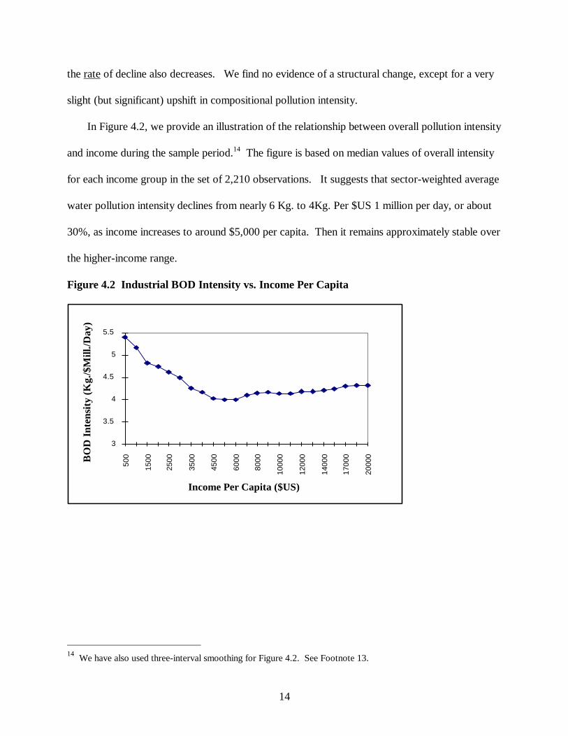
In Figure 4.2, we provide an illustration of the relationship between overall pollution intensity

and income during the sample period.14 The figure is based on median values of overall intensity

for each income group in the set of 2,210 observations. It suggests that sector-weighted average

water pollution intensity declines from nearly 6 Kg. to 4Kg. Per $US 1 million per day, or about

30%, as income increases to around $5,000 per capita. Then it remains approximately stable over

the higher-income range.

Figure 4.2 Industrial BOD Intensity vs. Income Per Capita

3

3.5

4

4.5

5

5.5

500

1500

2500

3500

4500

6000

8000

1000

0

1200

0

1400

0

1700

0

2000

0

Income Per Capita ($US)

BO

D I

nten

sity

(Kg.

/$M

ill./D

ay)

14 We have also used three-interval smoothing for Figure 4.2. See Footnote 13.

15

4.3 End-of-Pipe Pollution Intensity

Tables 4.3 - 4.5 report cross-country regression results for Equations (5) and (6). We use

dummy variables to control for sectoral differences in average pollution intensity; dummy variable

controls are also introduced for national differences in reporting procedures and measures of

organic water pollution. The majority of environmental protection agencies (EPA’s) have

reported emissions of biological oxygen demand (BOD), which is a measure of oxygen removal

from water by bacteria which are oxidizing organic materials. However, three EPA’s – for

China, Netherlands and Taiwan (China) – have reported COD (chemical oxygen demand). COD

incorporates the effect of other pollutants on the rate of oxidization; it is systematically larger than

BOD measures.

We have controlled for the measurement problem by introducing a dummy variable for COD-

based emissions reports. As expected, the estimated COD dummy is positive, large and highly

significant in all pollution intensity equations. Our sectoral dummy variable results are also in

accord with prior expectations: Food and Paper have the highest average organic water pollution

intensities; Metals and Mineral Products have the lowest. In the case of labor intensity, Textiles,

Food and Wood Products are highest (along with Other Manufacturing, the numeraire sector);

Metals and Chemicals are the lowest.

We have also controlled for the possible impact of differences in emissions reporting

procedures. In several cases (China, India, Indonesia, Netherlands, Philippines, Sri Lanka,

Taiwan (China), Thailand) the plant-level information provided by the EPA’s includes

employment data. This has enabled us to estimate sectoral pollution/labor ratios directly from the

EPA data. In the other cases (Brazil, Finland, Korea, Mexico and the US), the EPA’s have

provided summary pollution data by sector. We have obtained summary employment data by

16

sector from other national or regional sources, and have used the two summaries to calculate

sectoral pollution/labor ratios.

We recognize the possibility of systematic differences in the results generated by these two

approaches. EPA’s in developing countries focus on large polluters, so the average pollution

intensity of these facilities will be reflected in estimates based on plant samples. The situation is

potentially quite different when EPA-reported sectoral emissions are divided by census-reported

sectoral employment. Plants which ignore pollution regulations (and whose reported pollution is

therefore zero) may nevertheless be registered in an employment census. This might impart a

downward bias to summary-based intensities. In addition, all five countries for which we employ

summary data (Brazil, Finland, Korea, Mexico, US) are in the middle or high income category.

Thus, failure to control for the sampling difference might also produce a downward bias in the

estimated effect of income or wages on pollution intensity.

We have introduced a dummy variable to control for this difference, but it is not significant in

our regressions. In fact, we are not overly surprised by this result because effective coverage of

industrial facilities by both census-takers and regulators is a function of development.15

4.3.1 The Effects of Pollution Regulation and Relative Input Prices

As expected, the estimated wage-elasticity of labor intensity is large (around -.70) and highly

significant. The wage elasticity of pollution intensity is also negative, large (-1.71) and highly

significant. In the pollution intensity equation, our results are consistent with the hypothesis that

15 Both approaches may underestimate ‘true’ sectoral pollution intensities in developing countries, because

existing research suggests that medium and large plants have lower pollution per unit of output than smallerfacilities (ceteris paribus). Since smaller plants are covered by regulators in developed economies, oureconometric result may actually understate the effect of income on pollution intensity. We accept theplausibility of this hypothesis, but we have no way to test it at present.

17

labor and pollution are complements in production. However, the converse is not true. Our

index of regulatory strictness is not significant in the labor intensity equation.

While the latter result is not particularly surprising, we also find that our regulatory strictness

index is not significant in pollution intensity regressions which control for wages. Does this

imply that market forces alone drive pollution, and that regulation is irrelevant? Although our

results are consistent with this interpretation, we reject it for several reasons. First, our wage and

regulation variables are highly collinear because they are both correlated with per capita income.

As Table 4.4 shows, each variable is significant in equations which exclude the other. Second, a

large body of empirical work suggests that industrial pollution is responsive to pressure from local

communities (Pargal and Wheeler, 1996; Hettige, et. al., 1997, Hartman, et. al., 1996), as well as

formal regulation. Both forms of regulation are strongly affected by income, reflecting

increasing preferences for environmental quality and higher valuation of pollution damage. We

believe that the estimated wage elasticity in our pollution intensity regression is capturing cross-

country income effects on formal and informal regulation, as well as the effect of complementarity

with pollution in production. With currently-available information, we cannot distinguish clearly

between these two effects. However, their joint effect clearly shows the impact of rising income

on pollution intensity.

Our results for energy and capital prices are considerably weaker. Surprisingly, neither

variable is significant in the labor intensity equation when both are included. In the pollution

intensity regression, the estimated electricity price elasticity is positive, large and highly

significant. The real interest rate elasticity is also positive, and close to significance at the 5%

level. However, these results are not robust to changes in right-hand variables or sample

composition. Dropping the real interest rate increases the sample size, because we do not have

18

real interest rate data for Mexico, Brazil and Taiwan (China). However, with the larger sample

the electricity price elasticity loses significance in the pollution intensity equation, while becoming

large, negative, and highly ‘significant’ in the labor intensity equation. We conclude that our

results for capital and energy prices are highly sensitive to outliers, and we see no reason to draw

any clear conclusions from our results.

4.3.2 Economic Development and Pollution Intensity

We have also estimated reduced-form intensity equations which control for per capita

income, sector and COD reporting. The results are summarized in Table 4.5 for three intensities:

labor/output, pollution/output and pollution/labor. In all three equations, the results for the

sectoral dummies replicate the pattern of results in Tables 4.3-4.4. As before, the dummy variable

for COD is positive and significant in the pollution equations.

The results for per capita income suggest a striking regularity across countries. The income

elasticities of pollution/output and labor/output are both negative, and not significantly different

from one. In the third equation, we test for the equality of pollution and labor elasticities (w.r.t.

income) by regressing pollution/labor on the same set of right-hand variables (this amounts to

differencing the coefficients in the first two equations). The resulting elasticity of

pollution/labor with respect to income per capita is not significantly different from zero. Of

course, we cannot generalize from one sample for one pollutant to all industrial emissions.

However, for industrial water pollution, our results suggest that sectoral emissions/labor ratios

are approximately constant across countries at all income levels. Developing economies

generate much more pollution per unit of output than developed economies, but they also employ

much more labor per unit of output, and in the same proportion.

19

Figure 4.3 and Table 4.6 portray the estimated relationship between pollution intensity (per

unit of output) and income per capita. For ease of interpretation, we normalize to an intensity

value of 100 for the poorest income category ($500 per capita). The cross-country evidence

suggests a sharp drop in pollution intensity with income growth, as manufacturers respond to

higher wages and regulatory pressures with end-of-pipe abatement and process change. From an

emissions index value of 100 at $500 per capita, pollution abatement is about 60% at $1,500,

80% at $3,000, 90% at $7,000 and 95% at $15,000.

Table 4.6: Income and Pollution Abatement

IncomePer Capita

%Abatement

1,500 603,000 807,000 90

15,000 95

Figure 4.3: Water Pollution Intensity vs. Income Per Capita

0

10

20

30

40

50

60

70

80

90

100

0 2000 4000 6000 8000 10000 12000 14000 16000 18000 20000

Per Capita Income ($US)

Nor

mal

ized

Pol

lutio

n In

tens

ity

20

5. IMPLICATIONS OF THE RESULTS

5.1 The Kuznets Hypothesis

Our estimation exercises have suggested three distinct patterns of response to economic

development. Industry’s share of national output rises sharply through middle-income status and

then slowly declines. Sectoral composition follows a ‘clean’ trend for low-income developing

countries, but exhibits little or no trend beyond the middle income range. End-of-pipe pollution

intensity, by contrast, declines continuously with income.

We use simulation to project the net result of changes in these three factors. Our four

simulation variables are in columns 1-4 of Table 5.1. Column 1 includes a broad range of

incomes, from $US 500 to $US 20,000 per capita. Columns 2 and 3 replicate the information on

manufacturing output shares and average pollution intensities in Figures 4.1 and 4.2. Column 4

reproduces the pollution intensity index in Figure 4.3, re-normalized to one for the lowest income

level.

We assume a unit population for convenience, so income per capita also serves as a measure

of total output. We simulate the overall relationship between economic development and

industrial pollution by multiplying the four column entries in each row. The result combines the

effects of changes in total output, manufacturing share, sectoral composition, and end-of-pipe

pollution intensity. Column 5 and Figure 5.1 portray the total pollution estimate, which has been

normalized to an index value of 100 at the lowest income level. Our result suggests that the

inverted U-shaped story is only half right for industrial water pollution: Total emissions rise

sharply in the range [$500 - $7,000], but remain constant as income increases further.

21

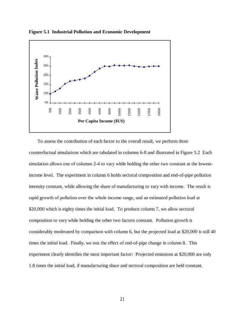
Figure 5.1 Industrial Pollution and Economic Development

50

100

150

200

250

300

500

1500

2500

3500

4500

6000

8000

1000

0

1200

0

1400

0

1700

0

2000

0

Per Capita Income ($US)

Wat

er P

ollu

tion

Inde

x

To assess the contribution of each factor to the overall result, we perform three

counterfactual simulations which are tabulated in columns 6-8 and illustrated in Figure 5.2 Each

simulation allows one of columns 2-4 to vary while holding the other two constant at the lowest-

income level. The experiment in column 6 holds sectoral composition and end-of-pipe pollution

intensity constant, while allowing the share of manufacturing to vary with income. The result is

rapid growth of pollution over the whole income range, and an estimated pollution load at

$20,000 which is eighty times the initial load. To produce column 7, we allow sectoral

composition to vary while holding the other two factors constant. Pollution growth is

considerably moderated by comparison with column 6, but the projected load at $20,000 is still 40

times the initial load. Finally, we test the effect of end-of-pipe change in column 8. This

experiment clearly identifies the most important factor: Projected emissions at $20,000 are only

1.8 times the initial load, if manufacturing share and sectoral composition are held constant.

22

We conclude that pollution levels off in the middle income range because end-of-pipe

pollution intensity responds to rising wages and stricter regulation. By comparison, the

manufacturing share and sectoral composition are minor players. For industrial water pollution,

the inverted-U pattern does not emerge because declining pollution intensity almost exactly

balances output growth, while manufacturing share and sectoral composition remain constant

beyond the middle income range.

Figure 5.2: Counterfactual Simulations

0

1,000

2,000

3,000

4,000

5,000

6,000

7,000

8,000

500

1500

2500

3500

4500

6000

8000

1000

0

1200

0

1400

0

1700

0

2000

0

Per Capita Income ($US)

Pollution Intensity

Manuf. Share

Sector Mix

Variable:

Wat

er P

ollu

tion

Inde

x

5.2 Trends in International Emissions

To explore the real-world implications of our results, we estimate pollution loads for a set of

large industrial economies during the period 1977 - 1989. Powerful leverage is provided by our

finding that sectoral pollution per unit of labor (P/L) remains approximately constant across the

entire range of incomes. This allows us to use commonly-available sectoral labor/output (L/Q)

ratios to predict international changes in industrial water pollution. As an illustration, we use the

World Bank’s BESD database to estimate sectoral L/Q ratios for fifteen countries during the

23

period 1977-1989. To estimate BOD loads by sector, we multiply the L/Q ratios by sectoral P/L

coefficients calculated from our regression results for P/L.16

We have chosen the fifteen countries to represent large industrial economies in four major

groups: OECD (represented by the US, Japan, France and Germany (former F.R.); the NIC’s

(Mexico, Brazil, Taiwan, Korea, South Africa, Turkey); Asian LDC’s (China, India, Indonesia);

and the ex-COMECON countries (Poland, former USSR). The results are tabulated in Table 5.3

(Appendix II) and summarized in Table 5.2 below. Taken together, they illustrate the main

implications of our empirical analysis.

In the OECD, despite modest continued economic growth, estimated BOD emissions remain

almost constant. In our view, this reflects the countervailing effects of output growth and

increases in wages and regulation; manufacturing shares and the ‘clean’ sector share change very

little. The COMECON economies are in relative stagnation during the sample period, so there is

little movement in their estimated emissions.

The story for the NIC’s is quite different. Their estimated pollution increases by about 25%

during the sample period – substantially less than their growth in per capita income. The increase

is relatively moderate because rapid output growth is offset by three factors: the negative impact

of increased wages and regulation on industrial pollution intensity; the first stage of the decline in

manufacturing share; and the last stage of the ‘clean’ trend in sectoral composition.

The Asian LDC experience is also distinctive. Estimated BOD emissions grow by

approximately 55% in these lower-income economies, because rapid output growth and

16 For this application, we regress log (P/L) on dummy variables for COD and the industry sectors. Since income

is insignificant, we impose a parameter value of zero by dropping it from the equation. To calculate sectoralP/L ratios, we assume the BOD case (COD=0), add the constant term to the estimated parameters for thesector dummies, and calculate the antilogs of the results.

24

increasing manufacturing share dominate the clean compositional trend and the first effects of

rising wages and regulation on pollution intensity. To a striking degree, BOD growth in our

international sample is due to increased emissions in developing Asia.

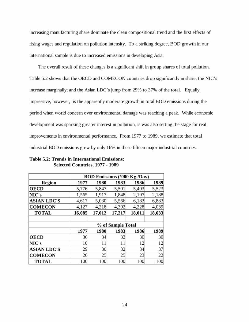
The overall result of these changes is a significant shift in group shares of total pollution.

Table 5.2 shows that the OECD and COMECON countries drop significantly in share; the NIC’s

increase marginally; and the Asian LDC’s jump from 29% to 37% of the total. Equally

impressive, however, is the apparently moderate growth in total BOD emissions during the

period when world concern over environmental damage was reaching a peak. While economic

development was sparking greater interest in pollution, is was also setting the stage for real

improvements in environmental performance. From 1977 to 1989, we estimate that total

industrial BOD emissions grew by only 16% in these fifteen major industrial countries.

Table 5.2: Trends in International Emissions: Selected Countries, 1977 - 1989

BOD Emissions (‘000 Kg./Day)Region 1977 1980 1983 1986 1989

OECD 5,776 5,847 5,501 5,403 5,523NIC's 1,565 1,917 1,848 2,197 2,188ASIAN LDC'S 4,617 5,030 5,566 6,183 6,883COMECON 4,127 4,218 4,302 4,228 4,039 TOTAL 16,085 17,012 17,217 18,011 18,633

% of Sample Total1977 1980 1983 1986 1989

OECD 36 34 32 30 30NIC's 10 11 11 12 12ASIAN LDC'S 29 30 32 34 37COMECON 26 25 25 23 22 TOTAL 100 100 100 100 100

25

6. SUMMARY AND CONCLUSIONS

In this paper, we have used new international data to investigate the relationship between

industrial pollution and economic development. To test for a Kuznets effect, we measure the

effect of income growth on three proximate determinants of pollution: The share of

manufacturing in total output; the sectoral composition of manufacturing; and the intensity (per

unit of output) of industrial pollution at the end-of-pipe. We find that the manufacturing share

follows a Kuznets-type trajectory, but the other two determinants do not. Sectoral composition

gets ‘cleaner’ through middle-income status and then stabilizes. At the end-of-pipe, pollution

intensity declines strongly with income. We attribute part of this to stricter regulation as income

increases, and partly to pollution-labor complementarity in production.

Our results suggest that income elasticities of both pollution- and labor-intensity are

approximately minus one. The remarkable implication is that a sector’s pollution/labor ratio is

constant across countries at all income levels. Our findings motivate two illustrative simulation

exercises. First, for a set of income benchmarks, we simulate total pollution by combining

representative measures of manufacturing share in output, sectoral composition, and end-of-pipe

pollution abatement. We do not see a Kuznets-type story in the result, since total pollution rises

rapidly through middle-income status and remains approximately constant thereafter. In three

counterfactual experiments, we assess the relative importance of the three proximate

determinants. Our results highlight the dominance of end-of-pipe reductions as wages and

regulation increase with development. The combined influence of changes in manufacturing share

and sectoral composition is lower by almost two orders of magnitude.

Our second simulation uses international panel data to explore the implications of constant

sectoral pollution/labor ratios. We estimate recent trends in water pollution for fifteen major

26

industrial nations in the OECD, the NIC’s, Asian LDC’s and the ex-COMECON economies. We

find approximately stable emissions in the OECD and ex-COMECON, moderate increases in the

NIC’s and rapidly-growing pollution in the Asian LDC’s. During the 1980’s, our estimates

suggest that the latter group displaced the major OECD economies as the world’s largest

generator of organic water pollution. Overall, however, the negative feedback from economic

development to pollution intensity was sufficient to hold total world pollution growth to around

15% during a twelve-year sample period.

In closing, it is worth asking whether these results are cause for optimism or pessimism. The

appropriate answer seems to be ‘both.’ It is comforting to see that industrial water emissions

level off in richer economies because pollution intensity has an elastic response to income growth.

Unfortunately, unitary elasticity implies that total emissions remain constant unless other factors

intervene. Of course, industry tends to deconcentrate over time as infrastructure improves and

prosperity spreads. Constant total emissions may therefore be consistent with improving water

quality in at least some areas. However, the continued existence of many seriously-polluted

waterways, even in the most prosperous countries, suggests that economic development remains

far short of a Kuznets-style happy ending in the water sector.

27

REFERENCES

Afsah, Shakeb, Benoit Laplante and David Wheeler, 1996, “Controlling Industrial Pollution: ANew Paradigm,” World Bank, Policy Research Department Working Paper

Beede, David, David Bloom and David Wheeler, 1992, “Measuring and Explaining Cross-Establishment Variation in the Generation and Management of Industrial Waste, World Bank(mimeo.)

Birdsall, Nancy and David Wheeler, 1993, “Trade Policy and Industrial Pollution in LatinAmerica: Where are the Pollution Havens? Journal of Environment and Development, 2, 1,Winter, 137-149.

Christensen, L., D. Jorgensen and L. Lau, 1973, “Transcendental Logarithmic ProductionFrontiers,” Review of Economics and Statistics, 55:28-45

Dasgupta, Susmita and David Wheeler, 1996, “Citizen Complaints as Environmental Indicators:Evidence from China,” World Bank, Policy Research Department Working Paper, December

Dasgupta, Susmita, Ashoka Mody, Subhendu Roy and David Wheeler, 1995, “EnvironmentalRegulation and Development: A Cross-Country Empirical Analysis," World Bank, PolicyResearch Department Working Paper, No. 1448, April

Dasgupta, Susmita, Mainul Huq, David Wheeler and C.H.Zhang, 1996, “Water PollutionAbatement by Chinese Industry: Cost Estimates and Policy Implications,” World Bank, PolicyResearch Department Working Paper

Grossman, Gene and Alan Krueger, 1995, “Economic Growth and the Environment,” QuarterlyJournal of Economics, May, 353-377

Gruver, G.W., 1976, “Optimal Investment in Pollution Control Capital in a Neoclassical GrowthContext,” Journal of Environmental Economics and Management, 5, 165-177.

Hartman, Raymond, Mainul Huq and David Wheeler, 1997, “Why Paper Mills Clean Up:Determinants of Pollution Abatement in Four Asian Countries,” World Bank, Policy ResearchDepartment Working Paper, Number 1710.

Hartman, Raymond, Manjula Singh and David Wheeler, 1997, “The Cost of Air PollutionAbatement,” Applied Economics (forthcoming)

Hettige, H., R.E.B. Lucas and D. Wheeler, 1992, “The Toxic Intensity of Industrial Production:Global Patterns, Trends and Trade Policy,” American Economic Review Papers andProceedings, 82, 478-481.

28

Hettige, Hemamala, Paul Martin, Manjula Singh and David Wheeler, 1995, "IPPS: The IndustrialPollution Projection System," World Bank, Policy Research Department Working Paper,February.

Hettige, Hemamala, Mainul Huq, Sheoli Pargal and David Wheeler, 1996, "Determinants ofPollution Abatement in Developing Countries: Evidence from South and Southeast Asia," 1996,World Development, December.

Hettige, Hemamala, Manjula Singh, Sheoli Pargal and David Wheeler, 1997, “Formal andInformal Regulation of Industrial Pollution: Evidence from the US and Indonesia,” World BankEconomic Review, Fall.

John, A. and R. Pecchenino, 1992, “An Overlapping Generations Model of Growth and theEnvironment,” Department of Economics, Michigan State University (mimeo.).

Levinson, Arik, 1996, “Environmental Regulations and Manufacturers’ Location Choices:Evidence from the Census of Manufactures,” Journal of Public Economics, 62, 5-29.

Mani, Muthukumara S. and David Wheeler, 1997, “In Search of Pollution Havens? DirtyIndustry in the World Economy, 1960-1995,” World Bank, Policy Research DepartmentWorking Paper (forthcoming)

Mani, Muthukumara S., 1996, “Environmental Tariffs on Polluting Imports: An Empirical Study,”Environmental and Resource Economics, 7, 391-411

Mody, Ashoka and David Wheeler, Automation and World Competition: New Technologies,Industrial Location, and Trade (London: Macmillan Press, 1990).

Pargal, S. and D. Wheeler, 1996, “Informal Regulation in Developing Countries: Evidence fromIndonesia,” Journal of Political Economy, December.

Robison, David H., 1988, “Industrial Pollution Abatement: The Impact on the Balance of Trade,”Canadian Journal of Economics, 21, 702-706.

Seldon, Thomas and Daqing Song, 1994, “Environmental Quality and Development: Is There aKuznets Curve for Air Pollution Emissions?” Journal of Environmental Economics andManagement, 27, 147-162.

Seldon, Thomas and Daqing Song, 1995, “Neoclassical Growth, the J Curve for Abatement, andthe Inverted U Curve for Pollution,” Journal of Environmental Economics and Management,29, 162-168.

Shafik, Nemat, 1994, “Economic Development and Environmental Quality: An EconometricAnalysis,” Oxford Economic Papers, 46, 757-773

29

Syrquin, Moshe, 1989, “Patterns of Structural Change,” in Handbook of DevelopmentEconomics, Vol. 1, H. Chenery and T.N. Srinivasan, eds., (Amsterdam: North-Holland)

Tobey, James A., 1990, “The Effects of Domestic Environmental Policies on Patterns of WorldTrade: An Empirical Test,” Kyklos 43, Fasc. 2, 191-209.

Wang, Hua and David Wheeler, 1996, “Pricing Industrial Pollution in China: An EconometricAnalysis of the Levy System,” World Bank, Policy Research Department Working Paper, No.1644.

Wheeler, David and Ashoka Mody, 1992, “International Investment Location Decisions: TheCase of U.S. Firms,” Journal of International Economics, 33, 57-76.

Wheeler, David, 1991, "The Economics of Industrial Pollution Control: An InternationalPerspective," 1991, World Bank, Industry and Energy Department Working Paper, No. 60,January.

30

Appendix I: DATA SOURCES

Brazil: The water pollution data for the Sao Paulo Metropolitan region of Brazil were collectedby CETESB, the environmental agency for Sao Paulo State. Our pollution estimates are based onCETESB’s 1250-plant database, which includes measures of BOD loads in kg/day. Thecorresponding employment data came from the Sao Paulo State Ministry of Labor, whichprovided 2-digit sectoral information from 1991 on nearly 41,000 plants and 2.15 million workers.

China: Water pollution data for China were obtained from the National Environmental ProtectionAgency (NEPA), which maintains a comprehensive database on major sources of industrialpollution in China. Our estimates are based on NEPA’s 1993 emissions data for 269 factoriesscattered throughout China.

Finland: The Finnish economic data, aggregated at the 3-digit ISIC level, were provided by theCentral Statistical Office, covering both white and blue collar workers for 1989. The pollutiondata were provided by the Industrial Waste Water Office of the National Board of Waters and theEnvironment. They cover water emissions in 1992 from 193 large water-polluting factories.

India: The India data are from the state of Tamil Nadu. Plant-level pollution data andemployment data for 1993-94 were provided by the Tamil Nadu Pollution Control Board, whichmonitors air and water pollution for all the manufacturing units in the state.

Indonesia: The Indonesia data came from two different sources. The plant-level emissions datawere provided by BAPEDAL, Indonesia's National Pollution Control Agency in the Ministry ofEnvironment. The economic data are from Indonesia’s Central Statistics Bureau (BPS).

Korea: Korean pollution data were provided by the National Pollution Control Agency. Theycover water emissions by 13,504 facilities in 1991. Complementary employment data have beendrawn from Korea’s National Statistical Yearbooks and the ILO’s International LaborStatistics, 1991.

Mexico: Data for water emissions in the Monterrey Metropolitan Area were provided by theState Water Monitoring Authority. The data cover emissions from 7,500 facilities in 1994.Complementary employment data were provided by Mexico’s Census Bureau (INEGI).

Netherlands: Water emissions and employment data for approximately 700 regularly-monitoredfacilities in 1990 were provided by the Emissions Inventory System maintained by the Ministry ofHousing, Spatial Planning and the Environment (VROM).

Philippines: Water emissions and employment data for factories in the Metro Manila Area(MMA) were provided the Philippines Department of Natural Resources (DENR) and the LagunaLake Development Authority.

31

Taiwan (China): Water emissions and employment data for 1,800 plants were provided by theWater Quality Protection division of the Taiwan Environment Protection Agency.

Thailand: Seatec International, a private-sector environmental consulting firm in Bangkok,provided plant-level data from two industrial estates in Rangsit and Suksawat. The datasetcontained information on water emissions and employment for approximately 450 facilities in1992.

Sri Lanka: Water pollution and employment data for Sri Lanka were obtained from a study ofwaste water treatment options for the Ekala/Ja-ela Industrial Estate, which includes 143 industrialestablishments with 21,000 employees. The data were collected by a joint project of the WorldBank’s Metropolitan Environment Improvement Program and the Sri Lankan Board ofInvestment. Ekala/Ja-Ela industrial estate is one of the two major industrial estates in Sri Lanka.

U.S.A.: The information for the United States were drawn from two main sources. The wateremissions data have been collected from regional databases which monitor industrial waterdischarges as part of the U.S. Environmental Protection Agency’s NPDES system. Employmentdata are from the U.S. Census Bureau’s Longitudinal Research Database.

32

Appendix II: Tables

Table 4.1: Log (Manufacturing Share of Total Output) vs. Log (Income Per Capita), 1975-1994*

IndependentVariables

OLS FixedEffects

RandomEffects

OLS FixedEffects

RandomEffects

Log Income 0.9195(2.483)

0.5147(1.815)

0.5726(2.076)

1.3585(7.934)

0.7719(6.815)

0.9402(8.323)

Log Income squared -0.0442-(1.796)

-0.04268-(2.185)

-0.0364-(1.923)

-0.0704-(6.446)

-0.05988-(8.772)

-0.0622-(8.988)

Log Income * Time 0.07527(1.993)

0.0450(3.126)

0.0511(3.456)

*** *** ***

Log Income squared* Time

-0.0045-(1.858)

-0.0028-(3.154)

-0.0032-(3.538)

*** *** ***

Time -0.3194-(2.196)

-0.1614-(2.762)

-0.1911-(3.205)

-0.0120-(4.224)

0.0146(6.612)

0.0062(3.190)

Constant -6.1460-(4.480)

-3.3256-(3.254)

-4.074-(4.095)

-7.9373-(12.013)

-4.2714-(8.897)

-5.3585-(11.415)

Number ofObservations

1136 1136 1136 1136 1136 1136

Number of TimePeriods

16 16 16 16 16 16

Adjusted R-squared 0.299 0.151 0.015 0.297 0.171 0.003* T-statistics in parentheses

Table 4.2: Log (Sector-Weighted BOD Intensity) vs. Log (Income Per Capita), 1975-1994*

IndependentVariables

OLS FixedEffects

RandomEffects

OLS FixedEffects

RandomEffects

Log Income 0.2846(1.018)

-0.3903-(3.566)

-0.3709-(3.427)

-0.0236-(0.184)

-0.5362-(12.719)

-0.5283-(12.616)

Log Income squared -0.0234-(1.321)

0.01749(2.459)

0.0164(2.344)

-0.0019-(0.249)

0.0269(11.050)

0.0267(10.974)

Log Income * Time -0.0117-(0.416)

-0.00736-(1.214)

-0.0071-(1.171)

*** *** ***

Log Income squared* Time

0.0009(0.578)

0.0005(1.398)

0.0004(1.374)

*** *** ***

Time 0.03203(0.278)

0.0319(1.232)

0.0300(1.161)

0.0034(2.166)

0.0055(6.402)

0.0051(6.351)

Constant 0.6935(0.633)

3.4369(8.168)

3.3470(8.035)

1.7679(3.373)

3.9912(21.143)

3.9435(20.989)

Number ofObservations

928 928 928 928 928 928

Number of TimePeriods

16 16 16 16 16 16

Adjusted R-squared 0.043 0.043 0.043 0.043 0.041 0.041* T-statistics in parentheses

33

Table 4.3: Intensity Equations for Pollution and Labor (in Prices and Regulation)

Dep. Var. – Log. of: Pollution/Output

Pollution/Output

Labor/Output

Labor/Output

Independent Variables Coef. t-stat. Coef. t-stat. Coef. t-stat. Coef. t-stat.Log Wage -1.714 -3.055** -0.015 -0.044 -0.711 -8.473** -0.379 -6.380**Log Brown Index 2.459 0.958 -2.995 -1.601 0.164 0.422 -1.467 -4.657**Log Electricity Price 6.123 3.684** 0.620 0.526 -0.098 -0.580 -0.564 -3.354**Log Real Interest Rate 0.455 1.903* 0.029 0.872COD 4.308 4.829** 2.406 2.559**Food 5.658 5.044** 4.511 3.940** -0.571 -3.817** -0.813 -4.239**Textiles 4.601 4.163** 3.932 3.449** -0.018 -0.125 -0.168 -0.881Wood Products 3.717 2.775** 3.103 2.176** -0.021 -0.140 0.053 0.280Paper 6.864 6.102** 4.946 4.318** -0.151 -1.006 -0.231 -1.205Chemicals 4.614 3.916** 3.236 2.785** -0.526 -3.320** -0.715 -3.669**Non-Metallic Minerals 1.290 1.118 1.023 0.879 -0.123 -0.823 -0.242 -1.263Metals 2.312 1.910* 0.988 0.828 -0.697 -4.383** -0.771 -3.903**Metal Products 3.538 3.063** 2.232 1.920* -0.278 -1.842* -0.502 -2.612**Constant -27.244 -2.466** -0.702 -0.096 -5.253 -3.162** 1.933 1.479Adjusted R-square 0.63 0.34 0.92 0.81Number of Observations 68 99 80 116

*** significant at 1% confidence level ** significant at 5% confidence level * significant at 10% confidence level

34

Table 4.4: Intensity Equations for Pollution and Labor (in Prices and Regulation)

Dep. Var. – Log of: Pollution/Output

Labor/Output

Pollution/Output

Labor/Output

Independent Variables Coef. t-stat. Coef. t-stat. Coef. t-stat. Coef. t-stat.Log Wage -1.211 -6.153 -0.666 -22.600Log Brown index -4.885 -5.052 -2.872 -14.642Log Electricity Price 5.634 3.565 -0.280 -1.223 3.765 2.384 -1.173 -3.871Log Real Interest Rate 0.370 1.668 0.025 0.807 0.234 0.957 -0.058 -1.27COD 4.375 4.923 -0.110 -0.852 4.125 4.32 -0.197 -1.071Food 5.485 4.959 -0.585 -3.979 5.073 4.278 -0.792 -3.767Textiles 4.586 4.153 -0.018 -0.124 4.556 3.842 -0.016 -0.074Wood Products 3.654 2.733 -0.028 -0.188 3.429 2.392 -0.131 -0.622Paper 6.675 6.032 -0.167 -1.132 6.222 5.247 -0.396 -1.882Chemicals 4.246 3.815 -0.558 -3.764 3.364 2.837 -1.023 -4.866Non-Metallic Minerals 1.114 0.979 -0.138 -0.941 0.681 0.558 -0.362 -1.720Metal s 2.014 1.723 -0.722 -4.729 1.243 0.999 -1.094 -5.045Metal Products 3.323 2.935 -0.296 -2.011 2.784 2.299 -0.560 -2.661Constant -16.903 -7.208 -4.403 -13.734 3.324 0.661 7.522 7.83Adjusted R-square 0.64 0.93 0.59 0.85Number ofObservations

68 80 68 80

35

Table 4.5: Intensity Equations for Pollution and Labor (in Income Per Capita)

Dep. Var. – Log of: Pollution/Output Labor/Output Pollution/LaborIndependent variables Coef. t-stat. Coef. t-stat. Coef. t-stat.Log Income -0.875 -3.26** -1.003 -17.041** 0.120 0.449COD 1.908 2.542** 1.930 2.576**Food 4.629 4.096** -0.925 -4.085** 5.492 4.868**Textiles 4.055 3.588** -0.150 -0.662 4.143 3.673**Wood Products 3.315 2.350** 0.047 0.206 3.485 2.475**Paper 5.064 4.481** -0.350 -1.547 5.353 4.745**chemical 3.349 2.963** -0.957 -4.225** 4.244 3.762**mineral 1.151 1.003 -0.361 -1.595 1.414 1.235metal 1.119 0.962 -0.964 -4.171** 2.038 1.786metal products 2.367 2.071** -0.635 -2.803** 2.983 2.615**constant -8.872 -3.615** -1.497 -2.828** -7.246 -2.972**Adjusted R-square 0.35 0.74 0.39Number ofObservations

99 116 100

Table 5.1: Industrial Pollution and Economic Development: Simulation Experiments

Income($US)

Manuf.Share

BODIntens.

EOPIntens.

TotalBOD

VariableShare

VariableBOD

VariableEOP

500 11.0 5.4 1.00 100 100 100 1001,500 13.4 4.8 0.39 128 366 268 1182,500 16.9 4.6 0.25 167 771 428 1273,500 18.5 4.3 0.19 177 1,179 553 1334,500 21.0 4.0 0.15 197 1,726 670 1386,000 24.3 4.0 0.12 237 2,663 888 1448,000 23.5 4.2 0.09 247 3,424 1,230 150

10,000 23.3 4.1 0.08 253 4,256 1,531 15512,000 22.6 4.2 0.07 255 4,953 1,859 16014,000 21.2 4.2 0.06 246 5,399 2,188 16317,000 20.3 4.3 0.05 248 6,298 2,709 16820,000 19.5 4.3 0.04 249 7,904 3,559 175

36

Table 5.3: Estimated Industrial BOD Emissions Selected Countries, 1977 - 1989 (‘000 Kg./Day)

COUNTRY 1977 1980 1983 1986 1989

UNITED STATES 2,652 2,743 2,551 2,454 2,564FRANCE 739 716 683 666 652GERMANY (FORMER FR) 929 932 800 789 800JAPAN 1,456 1,456 1,467 1,493 1,507 OECD 5,776 5,847 5,501 5,403 5,523

BRAZIL 611 867 771 965 914MEXICO 109 131 130 179 174KOREA, REPUBLIC OF 261 282 296 345 377TAIWAN, CHINA 208 239 252 296 282SOUTH AFRICA 226 238 245 245 262TURKEY 150 160 155 167 179 NIC's 1,565 1,917 1,848 2,197 2,188

CHINA 3,118 3,358 3,957 4,551 5,023INDIA 1,309 1,457 1,380 1,277 1,428INDONESIA 190 214 230 355 433 DEVELOPING ASIA 4,617 5,030 5,566 6,183 6,883

POLAND 578 581 546 484 459U.S.S.R., FORMER 3,549 3,638 3,756 3,744 3,580 EX-COMECON 4,127 4,218 4,302 4,228 4,039

TOTAL 16,085 17,012 17,217 18,011 18,633

THE WORLD BANK/IFC/M.I.G.A.

OFFICE MEMORANDUM

DATE: December 5, 1997

TO: Gregory Ingram, Administrator, RAD

THROUGH: Zmarak Shalizi, Research Manager, DECRG

FROM: David Wheeler, Principal Economist, DECRG

EXTENSION: 33401

SUBJECT: Submission for Policy Research Working Paper Series

Please find enclosed a copy of the paper, “Industrial Pollution in Economic Development:Kuznets Revisited,” which we would like to submit to the Policy Research Working PaperSeries. As far as we know, this is the first empirical assessment of the relationship betweendevelopment and industrial emissions which uses actual plant-level water pollution data fromdeveloping countries. The paper analyzes the impact of relative input prices, regulation andincome on three proximate determinants of total pollution: The share of manufacturing innational output; the sectoral composition of manufacturing; and industrial emissionsintensity at the end-of-pipe. The paper tests for Kuznets-type effects in each dimension, andcombines the evidence in an assessment of the overall relationship between pollution anddevelopment.

This paper should be of interest to the international environmental policy community, Bankenvironment professionals, and other staff members who are working on industrial andregulatory issues. It has been reviewed by Professor Judith Dean of SAIS and a number ofcolleagues in the World Bank. We believe that country clearance is not necessary, since thisis an international study which does not report results for individual countries.

Enclosures:

Draft working paper and abstractDiskette with Word files

cc: Messrs./Mmes. Pleskovic, Else (RAD); Squire (DECVP); Shalizi, Guido-Spano(DECRG); Mani (EDI); Hettige (ADB)