Inductive Voltage Transformers Calibration by the...

Inductive Voltage Transformers Calibration by the ParametersAUGUSTO F BRANDÃO JR, IZAEL P DA SILVA, ANTONIO C DE SILOS, DIMETRI IVANOV,

EDUARDO M DIASElectric Power and Automation Engineering Department

Polytechnic School of the University of São PauloAv. Professor Luciano Gualberto, 158, Trav. 3, São Paulo - SP

[email protected], [email protected], [email protected], [email protected]

Abstract: - The accuracy class of an IVT – Inductive Voltage Transformer – is typically assessed in laboratory installations either by comparing with another IVT presenting greater accuracy and traceable to a national laboratory or by using a capacitive divider. Calibration in the field using internal parameters is considered herein, using results obtained from typical open and short circuit tests and winding resistances, performed with common meters. A Möllinger & Gewecke graphic diagram is employed together with the results of an accuracy test previously carried out to determine the exact value of the winding turn relation and of the primary winding dispersion reactance. These values are used to calculate the phase and ratio errors, which must lie between definite limits, defined by the accuracy class of the instrument. Four commercial IVTs were tested to determine the validity of the procedure. The errors are compared with those obtained with the Schering-Alberti method (AC Bridge and comparison with standard IVT).

Keywords: - Instrument Transformers, Inductive Voltage Transformer, Voltage Transducers, Measurement Errors, Error Estimation, Certification, Calibration

1. IntroductionIn an ideal instrument transformer, the voltage

quantity at the terminals of the secondary is identical to that of the primary winding in a reduced scale, presenting no phase difference. However, a real IVT - Inductive Voltage Transformer - presents divergences not only in the magnitude but also in the phases of voltages, errors that change with the burden of the instrument transformer. The current formulae for the errors require the values of the primary dispersion reactance calculated separately as well as the exact winding turn relation. The difficulty in obtaining these values probably explains the infrequent use of the analytical method in verifying IVTs accuracy class, which must be within ranges of 0.1 to 0.3%, for purposes of electrical energy billing. To accomplish this, comparative methods are normally employed in laboratories, using standard AC bridges.

The objective of this paper is to demonstrate a practical method for verifying the accuracy of commercial IVTs with typical open and short circuit tests, performed with common instruments in the field. Consequently, inconvenient and troublesome transportation to a laboratory facility for verification is avoided. A graph method employing the Möllinger & Gewecke diagram allows for determining the separate primary winding reactance, as well as the

compensation value. With these values, it is possible to calculate the errors and verify the accuracy class of the transformer. The IVTs considered here are for distribution networks, with rated primary voltages up to 34.5 kV (phase to phase) and 34.5/√3 (phase to neutral). The common classes are of 15 kV, 25 kV and 36 kV, installed in substations supplying industrial and commercial loads, connected to measurement devices. In the case of higher voltages, in the range of hundreds of kVs used in transmission and sub transmission networks, CVTs – capacitive voltage transformers are more commonly employed. However, their construction is based on a capacitive divider connected to an inductive voltage transformer, therefore this process also applies to CVTs.

2. Accuracy Classes of IVT'sAccording to the standards [1,2], the accuracy

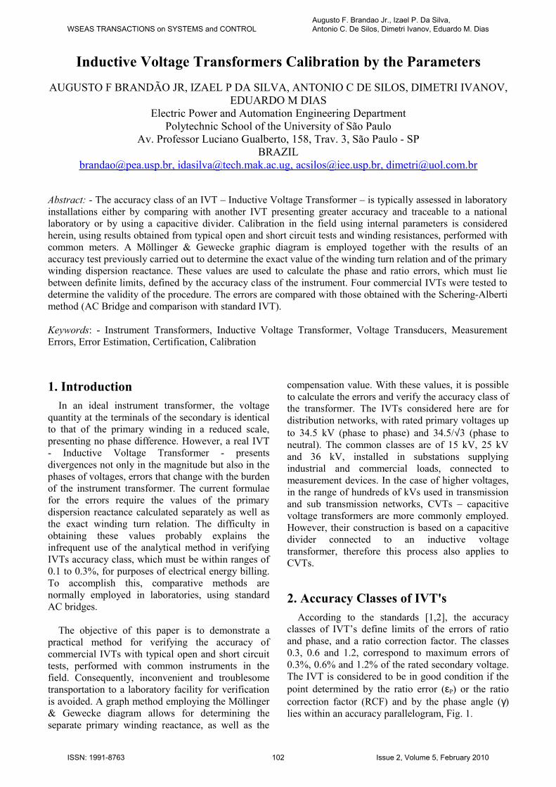
classes of IVT’s define limits of the errors of ratio and phase, and a ratio correction factor. The classes 0.3, 0.6 and 1.2, correspond to maximum errors of 0.3%, 0.6% and 1.2% of the rated secondary voltage. The IVT is considered to be in good condition if the point determined by the ratio error (εP) or the ratio correction factor (RCF) and by the phase angle (γ) lies within an accuracy parallelogram, Fig. 1.

WSEAS TRANSACTIONS on SYSTEMS and CONTROLAugusto F. Brandao Jr., Izael P. Da Silva, Antonio C. De Silos, Dimetri Ivanov, Eduardo M. Dias

ISSN: 1991-8763 102 Issue 2, Volume 5, February 2010

mailto:[email protected]

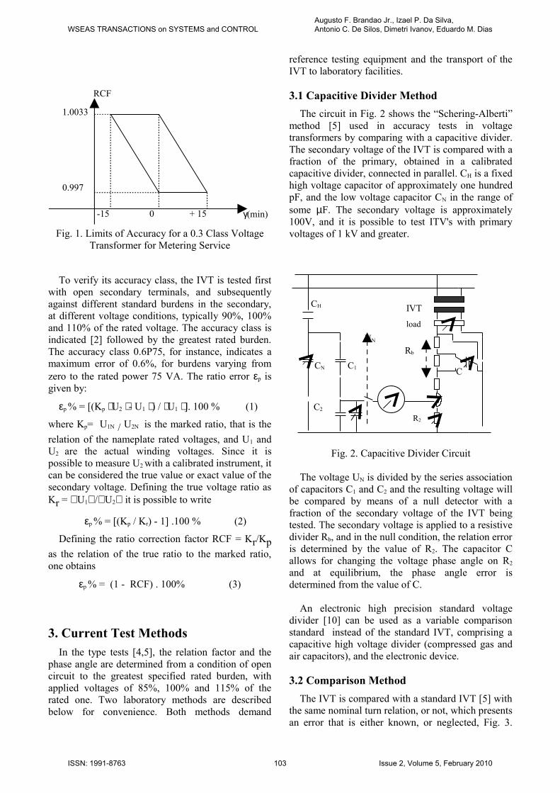
Fig. 1. Limits of Accuracy for a 0.3 Class Voltage Transformer for Metering Service

To verify its accuracy class, the IVT is tested first with open secondary terminals, and subsequently against different standard burdens in the secondary, at different voltage conditions, typically 90%, 100% and 110% of the rated voltage. The accuracy class is indicated [2] followed by the greatest rated burden. The accuracy class 0.6P75, for instance, indicates a maximum error of 0.6%, for burdens varying from zero to the rated power 75 VA. The ratio error εp is given by:

εp % = [(Kp U2 - U1 ) / U1 ]. 100 % (1)

where Kp= U1N / U2N is the marked ratio, that is the relation of the nameplate rated voltages, and U1 and U2 are the actual winding voltages. Since it is possible to measure U2 with a calibrated instrument, it can be considered the true value or exact value of the secondary voltage. Defining the true voltage ratio as Kr = U1/U2 it is possible to write

εp % = [(Kp / Kr) - 1] .100 % (2)

Defining the ratio correction factor RCF = Kr/Kp as the relation of the true ratio to the marked ratio, one obtains

εp % = (1 - RCF) . 100% (3)

3. Current Test MethodsIn the type tests [4,5], the relation factor and the

phase angle are determined from a condition of open circuit to the greatest specified rated burden, with applied voltages of 85%, 100% and 115% of the rated one. Two laboratory methods are described below for convenience. Both methods demand

reference testing equipment and the transport of the IVT to laboratory facilities.

3.1 Capacitive Divider Method The circuit in Fig. 2 shows the “Schering-Alberti”

method [5] used in accuracy tests in voltage transformers by comparing with a capacitive divider. The secondary voltage of the IVT is compared with a fraction of the primary, obtained in a calibrated capacitive divider, connected in parallel. CH is a fixed high voltage capacitor of approximately one hundred pF, and the low voltage capacitor CN in the range of some µF. The secondary voltage is approximately 100V, and it is possible to test ITV's with primary voltages of 1 kV and greater.

Fig. 2. Capacitive Divider Circuit

The voltage UN is divided by the series association of capacitors C1 and C2 and the resulting voltage will be compared by means of a null detector with a fraction of the secondary voltage of the IVT being tested. The secondary voltage is applied to a resistive divider Rb, and in the null condition, the relation error is determined by the value of R2. The capacitor C allows for changing the voltage phase angle on R2

and at equilibrium, the phase angle error is determined from the value of C.

An electronic high precision standard voltage divider [10] can be used as a variable comparison standard instead of the standard IVT, comprising a capacitive high voltage divider (compressed gas and air capacitors), and the electronic device.

3.2 Comparison Method The IVT is compared with a standard IVT [5] with

the same nominal turn relation, or not, which presents an error that is either known, or neglected, Fig. 3.

CH

CN C1

C2

IVT

load

R2

C

UN

Rb

RCF

γ(min)

1.0033

0.997

-15 0 + 15



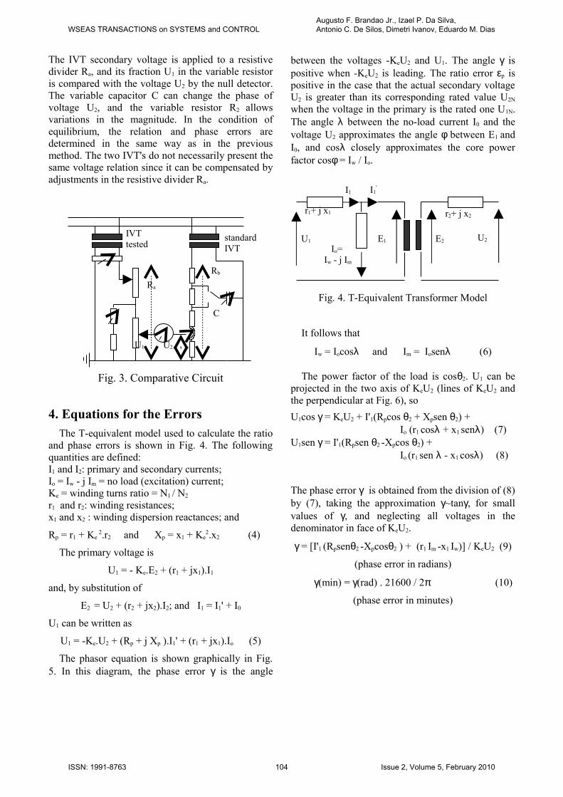
The IVT secondary voltage is applied to a resistive divider Ra, and its fraction U1 in the variable resistor is compared with the voltage U2 by the null detector. The variable capacitor C can change the phase of voltage U2, and the variable resistor R2 allows variations in the magnitude. In the condition of equilibrium, the relation and phase errors are determined in the same way as in the previous method. The two IVT's do not necessarily present the same voltage relation since it can be compensated by adjustments in the resistive divider Ra.

Fig. 3. Comparative Circuit

4. Equations for the Errors

The T-equivalent model used to calculate the ratio and phase errors is shown in Fig. 4. The following quantities are defined:I1 and I2: primary and secondary currents;Io = Iw - j Im = no load (excitation) current;

Ke = winding turns ratio = N1 / N2

r1 and r2: winding resistances; x1 and x2 : winding dispersion reactances; and

Rp = r1 + Ke 2.r2 and Xp = x1 + Ke

2.x2 (4)

The primary voltage is

U1 = - Ke.E2 + (r1 + jx1).I1

and, by substitution of

E2 = U2 + (r2 + jx2).I2; and I1 = I1' + I0

U1 can be written as

U1 = -Ke.U2 + (Rp + j Xp ).I1' + (r1 + jx1).Io (5)

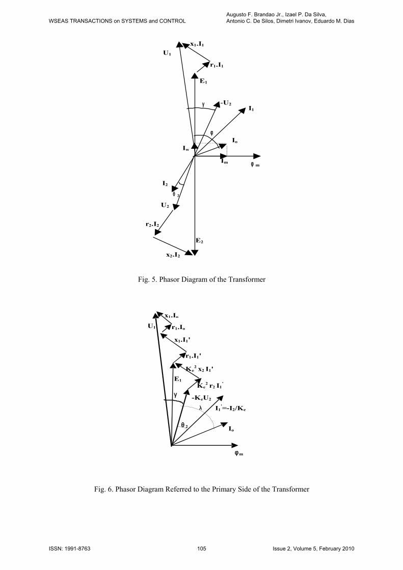
The phasor equation is shown graphically in Fig. 5. In this diagram, the phase error γ is the angle

between the voltages -KeU2 and U1. The angle γ is positive when -KeU2 is leading. The ratio error εp is positive in the case that the actual secondary voltage U2 is greater than its corresponding rated value U2N

when the voltage in the primary is the rated one U1N. The angle λ between the no-load current I0 and the voltage U2 approximates the angle φ between E1 and I0, and cosλ closely approximates the core power factor cosφ = Iw / Io.

Fig. 4. T-Equivalent Transformer Model

It follows that

Iw = Iocosλ and Im = Iosenλ (6)

The power factor of the load is cosθ2. U1 can be projected in the two axis of KeU2 (lines of KeU2 and the perpendicular at Fig. 6), soU1cos γ = KeU2 + I'1(Rpcos θ2 + Xpsen θ2) + Io (r1 cosλ + x1 senλ) (7) U1sen γ = I'1(Rpsen θ2 -Xpcos θ2) + Io (r1 sen λ - x1 cosλ) (8)

The phase error γ is obtained from the division of (8) by (7), taking the approximation γ~tanγ, for small values of γ, and neglecting all voltages in the denominator in face of KeU2.

γ = [I'1 (Rpsenθ2 -Xpcosθ2 ) + (r1 Im -x1 Iw)] / KeU2 (9)

(phase error in radians)

γ(min) = γ(rad) . 21600 / 2π (10)

(phase error in minutes)

r1+ j x1 r2+ j x2

Io= Iw - j Im

U2U1

I1 I1'

IVTtested

Ra

Rb

standard IVT

U1 U2

C

E2E1



Im

Iw

φ m

Io

U1

E1

-U2I1

I2

U2

r1.I1

x1.I1

r2.I2

γ

x2.I2

E2

θ 2

φ

Fig. 5. Phasor Diagram of the Transformer

Fig. 6. Phasor Diagram Referred to the Primary Side of the Transformer

φ m

Io

U1

E1

-KeU2 I1

'=-I2/Ke

r1.I1'

x1.I1'

γ Ke

2 r2 I1

'

Ke2

x2 I1'

r1.Io

x1.Io

θ 2

λ



Dividing (5) by U2, the true voltage relation Kr is obtained.

U1 / U2 = Kr = Ke + [I'1 (Rpcos θ2+Xpsen θ2) +

Io(r1cos λ+ x1sen λ)]/U2

(11)

and

Kr =

Ke + [I'1(Rpcos θ2 + Xpsen θ2)+(r1 Iw + x1 Im)]/ U2

(true voltage relation) (12)

From equation (2), the ratio error εp follows. The IVT compensation, whenever it exists, is included

in the value of Ke. The phase and ratio errors originate in two voltage drops: the first is due to the excitation current I0 that flows only in the primary winding; and the second is due to the burden current I'1 flowing in both windings, and depends on the burden connected and its power factor. The point here is that to calculate the errors the knowledge of the transformer parameters is necessary. The resistance of the primary winding has a high value and can be easily measured, while the resistance of the secondary demands a measuring bridge. From open circuit tests, the rms values of I0, Iw and Im are obtained within a precision of 1% with typical common meters. From short circuit tests, the values of RP and XP can be calculated.

Fig. 7 Mollinger & Gewecke Diagram



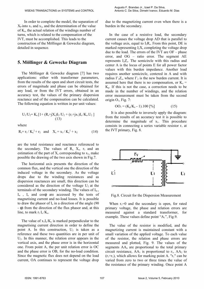
In order to complete the model, the separation of XP into x1 and x2, and the determination of the value of Ke, the actual relation of the windings number of turns, which is related to the compensation of the IVT, must be accomplished. This leads to the construction of the Möllinger & Gewecke diagram, detailed in sequence.

5. Möllinger & Gewecke Diagram

The Möllinger & Gewecke diagram [7] has two applications: either with transformer parameters, from the results of the open and short circuit tests, the errors of magnitude and phase can be obtained for any load, or from the IVT errors, obtained in an accuracy test, the values of the primary dispersion reactance and of the compensation can be calculated. The following equation is written in per unit values:

U1/U2= Ke [1+ (Rs+jXs)I2 /U2 + (r1+jx1)Io /Ke.U2 ] (13)

where

Rs= r1 / Ke2 + r2 and Xs = x1 / Ke

2 + x2 (14)

are the total resistance and reactance referenced to the secondary. The values of Rs, Xs, r1 and an estimation of the part of Xs corresponding to x1, make possible the drawing of the two axis shown in Fig.7.

The horizontal axis presents the direction of the common flux, and the vertical one the direction of the induced voltage in the secondary. As the voltage drops due to the winding resistances and as dispersion reactances are small, this direction can be considered as the direction of the voltage U2 at the terminals of the secondary winding. The values of Im , Iw , Io and cosφ are accessed by the tests of magnetising current and no-load losses. It is possible to draw the phasor of Io in a direction of the angle (90 - φ) from the direction of the flux phasor and, at this line, to mark r1 Io /Ke.

The value of x1Io/Ke is marked perpendicular to the magnetising current direction in order to define the point A. In this construction, U2 is taken as a reference and these two quantities are in per unit of U2. In this manner, the relation error appears in the vertical axis, and the phase error is in the horizontal one. From point A, the per unit relation error is OC and the phase error is OB, for the no-load condition. Since the magnetic flux does not depend on the load current, OA continues to represent the voltage drop

due to the magnetizing current even when there is a burden in the secondary.

In the case of a resistive load, the secondary current causes the voltage drop AD that is parallel to the voltage axis, equal to I2Rs. From this point, DE is marked representing I2Xs completing the voltage drop due to the load. The errors of the IVT are OF – phase error, and OG – ratio error. The segment AE represents I2Zs. The semicircle with this radius and center A is the locus of points E for all power factor values with this burden impedance. Another load requires another semicircle, centered in A and with radius I’2Zs, where I’2 is the new burden current. It is assumed here that there is no compensation, or Ke = Kp. If this is not the case, a correction needs to be made in the number of windings, and the relation error measurement must be taken from the second origin O1, Fig. 7:

OO1 = (Kp/Ke - 1).100 [%] (15)

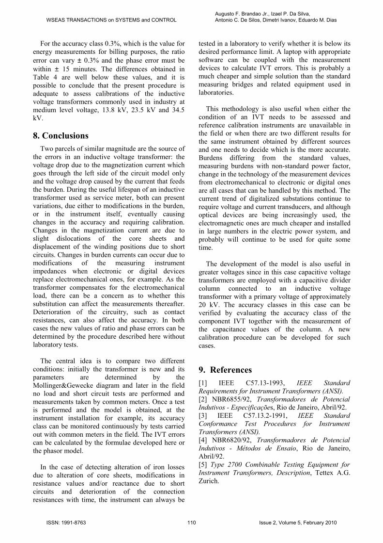
It is also possible to inversely apply the diagram: from the results of an accuracy test it is possible to determine the magnitude of x1. This procedure consists in connecting a series variable resistor rv at the IVT primary, Fig. 8.

Fig.8. Circuit for the Dispersion Measurement

When rv=0 and the secondary is open, for rated primary voltage, the phase and relation errors are measured against a standard transformer, for example. These values define point “A1”, Fig.9.

The value of the resistor is modified, and the magnetizing current is maintained constant with a small variation of the applied voltage. To each value of the resistor, the relation and phase errors are measured and plotted, Fig. 9. The values of the segments AAn are proportional to the total primary circuit resistance, AA1 is proportional to r1, AA2 to (r1+rv), which allows for marking point A. "rv" can be varied from zero to two or three times the value of the resistance of the primary winding. Once point A



has been established, a perpendicular is traced from it till it cuts the vertical axis (point “O”) thus defining both the regulation OO1 and the primary dispersion reactance x1.

Fig.9. Determination of x1 and the Compensation

6. Methodology [8]As the accuracy level depends only on the

geometric construction characteristics of the transformer and on the material used for the core and windings, the accuracy characteristics of the transformer will not be altered if these conditions are not changed. Short circuits can modify the relative position of the windings, but this rarely occurs in a voltage transformer. The magnetization and short circuit tests are sufficient for detecting any alteration in the characteristics mentioned above.

An accuracy test has to be previously carried out to determine the exact value of the winding turn's relation and primary winding dispersion reactance. This test can be performed in the laboratory by comparing the IVT with a standard one. The resistances of the primary and secondary windings are measured with the precision of common

ohmmeters, generally in the range of 1%. Normally, the primary winding presents a relatively high and easily measurable resistance; for the secondary, the value is in the range of mΩ, and the Kelvin Bridge is used. The magnetization and short circuit tests are performed in sequence [3]. The secondary is connected to the voltage source with open primary. The voltage is increased to the rated value and the magnetization current and the losses are determined. The short circuit tests are performed with the current corresponding to the greatest accuracy load divided by the winding rated voltage, measuring the voltage and the current. In the case of very low readings for the values, this test can be performed with the apparent thermal power divided by the rated voltage.

Finally, an accuracy test of the IVT is performed with a standard voltage transformer and the Schering-Alberti Bridge, initially with no load. The errors are measured with a known resistor, connected in series with the primary winding. The value of the compensation in the number of windings and the separate values of the dispersion reactance values can be calculated. The model is now complete and the errors can be calculated either by the formulae given in item IV or using phasor calculations as in the model of Fig. 4.

7. Measurements for ValidationFour inductive voltage transformers with different

accuracy classes, different voltage levels and different designs were tested in the Technical Measurements Laboratory of IEE/USP. Their nominal characteristics are presented in Table 1. The tests were made to determine the model parameters, the no-load test by the low voltage winding, the short circuit test by the high voltage winding: the results are shown in Table 2. Table 3 presents the results of the accuracy tests as well as the calculated values of the regulation and primary winding dispersion reactance.

Table 1 – Plate Characteristics of the IVT's

Transf.No.

brand Rated Primary Voltage (V)

Rated Second. Voltage (V)

Rated Frequency (Hz)

Thermal RatedVA

AccuracyClass

01 A 14,400 120 60 1400 0.3WXYZ-1.2ZZ02 B 4,600 115 60 500 0.3P2503 C 1,200 200 60 400 0.2P12.504 D 600 100 60 400 0.2P12.5



Table 2 – Tests to Obtain the Parameters for the Model

Table 3 – Tests to Obtain the Regulation and x1

Transf.No. Load / power factor

Measured - AC Bridge εp(%) γ(min)

Calculated Errors εp(%) γ(min)

Differences (calc-meas) ∆εp(%) ∆γ(min)

01020304

No-load0.23 0.6 0.23 0.68 0.00 +0.080.28 1.4 0.28 1.73 0.00 +0.330.07 0.86 0.06 0.88 -0.01 +0.020.15 0.3 0.15 0.28 0.00 -0.02

01020304

12.5 VA0.1 0.21 1.1 0.20 1.14 -0.01 +0.040.1 0.23 3.0 0.22 3.49 -0.01 +0.490.1 0.03 2.1 0.02 2.25 -0.01 +0.150.1 0.10 2.9 0.10 4.3 0.00 +1.4

0102 25 VA

0.7 0.18 0.4 0.17 0.43 -0.01 +0.030.7 0.13 1.3 0.12 1.67 -0.01 +0.37

Table 4 – Errors Measured in the Conventional AC Bridge and Calculated by Paper Equations

The accuracy tests were carried out by the comparative method against a standard voltage transformer of the class 0.05% using AC Bridge (Schering-Alberti method) and are presented in Table 4. The equipment employed was TETTEX type 2711/22 as the AC bridge for comparison with the standard IVT and the algebraic method [3] to determine the correction factor for relation and phase angle of the load. The secondary voltage was maintained as 100% of the rated value. This Table

also presents a comparison between the errors calculated by the equations and the experimental values. The differences are less than 0.05% for the ratio error and less than 0.5minute for the phase error. These values, 0.05% for the ratio error and 0.5minute for the phase error, are the margin errors commonly employed in standard bridges for calibration of IVT's.

Transf No.

Accuracy Test, no rv

εp (%) γ(min)Accuracy Test, with rv

εp (%) γ(min) rv (Ω)Calculated Values

regulation(%) x1 (Ω)01 0.23 0.6 0.21 2.5 3500 0.241 261.802 0.28 1.4 0.17 7.4 835 0.409 353.303 0.07 0.86 0.04 2.86 30 0.157 30.0604 0.15 0.3 0.13 0.7 20 0.172 2.839

TransfNo.

Winding ResistancesPrim.(Ω) Sec(mΩ)

No-load test, by the Secondaryvoltage (V) current(mA) power(W)

Short circuit test, Primaryvoltage (V) current.(mA)

01 1200 96.37 120 357.5 19.52 120.75 27.902 417.5 343 115 464 25.4 152 108.803 28.4 611 200 167.5 15.7 21.84 33304 19.88 420.2 100 41.0 3.575 24.30 666.7



For the accuracy class 0.3%, which is the value for energy measurements for billing purposes, the ratio error can vary ± 0.3% and the phase error must be within ± 15 minutes. The differences obtained in Table 4 are well below these values, and it is possible to conclude that the present procedure is adequate to assess calibrations of the inductive voltage transformers commonly used in industry at medium level voltage, 13.8 kV, 23.5 kV and 34.5 kV.

8. ConclusionsTwo parcels of similar magnitude are the source of

the errors in an inductive voltage transformer: the voltage drop due to the magnetization current which goes through the left side of the circuit model only and the voltage drop caused by the current that feeds the burden. During the useful lifespan of an inductive transformer used as service meter, both can present variations, due either to modifications in the burden, or in the instrument itself, eventually causing changes in the accuracy and requiring calibration. Changes in the magnetization current are due to slight dislocations of the core sheets and displacement of the winding positions due to short circuits. Changes in burden currents can occur due to modifications of the measuring instrument impedances when electronic or digital devices replace electromechanical ones, for example. As the transformer compensates for the electromechanical load, there can be a concern as to whether this substitution can affect the measurements thereafter. Deterioration of the circuitry, such as contact resistances, can also affect the accuracy. In both cases the new values of ratio and phase errors can be determined by the procedure described here without laboratory tests.

The central idea is to compare two different conditions: initially the transformer is new and its parameters are determined by the Mollinger&Gewecke diagram and later in the field no load and short circuit tests are performed and measurements taken by common meters. Once a test is performed and the model is obtained, at the instrument installation for example, its accuracy class can be monitored continuously by tests carried out with common meters in the field. The IVT errors can be calculated by the formulae developed here or the phasor model.

In the case of detecting alteration of iron losses due to alteration of core sheets, modifications in resistance values and/or reactance due to short circuits and deterioration of the connection resistances with time, the instrument can always be

tested in a laboratory to verify whether it is below its desired performance limit. A laptop with appropriate software can be coupled with the measurement devices to calculate IVT errors. This is probably a much cheaper and simple solution than the standard measuring bridges and related equipment used in laboratories.

This methodology is also useful when either the condition of an IVT needs to be assessed and reference calibration instruments are unavailable in the field or when there are two different results for the same instrument obtained by different sources and one needs to decide which is the more accurate. Burdens differing from the standard values, measuring burdens with non-standard power factor, change in the technology of the measurement devices from electromechanical to electronic or digital ones are all cases that can be handled by this method. The current trend of digitalized substations continue to require voltage and current transducers, and although optical devices are being increasingly used, the electromagnetic ones are much cheaper and installed in large numbers in the electric power system, and probably will continue to be used for quite some time.

The development of the model is also useful in greater voltages since in this case capacitive voltage transformers are employed with a capacitive divider column connected to an inductive voltage transformer with a primary voltage of approximately 20 kV. The accuracy classes in this case can be verified by evaluating the accuracy class of the component IVT together with the measurement of the capacitance values of the column. A new calibration procedure can be developed for such cases.

9. References[1] IEEE C57.13-1993, IEEE Standard Requirements for Instrument Transformers (ANSI).[2] NBR6855/92, Transformadores de Potencial Indutivos - Especificações, Rio de Janeiro, Abril/92.[3] IEEE C57.13.2-1991, IEEE Standard Conformance Test Procedures for Instrument Transformers (ANSI).[4] NBR6820/92, Transformadores de Potencial Indutivos - Métodos de Ensaio, Rio de Janeiro, Abril/92.[5] Type 2700 Combinable Testing Equipment for Instrument Transformers, Description, Tettex A.G. Zurich.



[6] B.Hague, Instrument Transformers: Their Theory, Characteristics and Testing, Sir Isaac Pitman and Sons Ltd., London, 1936.[7] Möllinger,J & Gewecke,H, Zum Diagramm des Stromwandlers, Elektrotechnische Zeitschrift (V.D.E. - Verlag ) vol. 33, 1912, pp 270-271.[8] I.P.Silva, Uma Proposta de Verificação da Classe de Exatidão de Transformadores de Potencial Indutivos, PhD Thesis, Polytechnic School of the University of São Paulo, 1997.[9] A.F.Brandão Jr et alli, "A Method for Cheking in the Field the Precision Class of Inductive Voltage Transformers", Eleventh International Symposium on High Voltage Engineering - ISH 99, London, 1999, Conference Proceedings pp 1.209-212.[10] Electronic high precision standard voltage dividers, Tettex instruments, P 4860-05.94.



Inductive Voltage Transformers Calibration by the...

Documents

Transcript of Inductive Voltage Transformers Calibration by the...