Indoor UAV control using multi-camera visual feedback · Indoor UAV control using multi-camera...
30
•
Transcript of Indoor UAV control using multi-camera visual feedback · Indoor UAV control using multi-camera...

Loughborough UniversityInstitutional Repository
Indoor UAV control usingmulti-camera visual feedback
This item was submitted to Loughborough University's Institutional Repositoryby the/an author.
Citation: OH, H. ... et al, 2011. Indoor UAV control using multi-cameravisual feedback. Journal of Intelligent and Robotic Systems, 61 (1-4), pp. 57 -84.
Additional Information:
• This article was published in the serial, Journal of Intelligent and RoboticSystems [ c© Springer Science+Business Media B.V.]. The final publicationis available at Springer via: http://dx.doi.org/10.1007/s10846-010-9506-8
Metadata Record: https://dspace.lboro.ac.uk/2134/17856
Version: Accepted for publication
Publisher: c© Springer Science+Business Media B.V.
Rights: This work is made available according to the conditions of the Cre-ative Commons Attribution-NonCommercial-NoDerivatives 4.0 International(CC BY-NC-ND 4.0) licence. Full details of this licence are available at:https://creativecommons.org/licenses/by-nc-nd/4.0/
Please cite the published version.

1
Indoor UAV Control Using Multi-camera
Visual Feedback
Hyondong Oh*, Dae-Yeon Won, Sung-Sik Huh, David Hyunchul Shim and Min-
Jea Tahk**, Antonios Tsourdos*
*Dept. of Informatics and Systems Engineering, Cranfield University, Swindon, UK
**Dept. of Aerospace Engineering, KAIST, Daejeon, South Korea
[email protected], [email protected], [email protected], [email protected],
[email protected], [email protected]
Abstracts This paper presents the control of an indoor unmanned aerial vehicle (UAV) using
multi-camera visual feedback. For the autonomous flight of the indoor UAV, instead of using
onboard sensor information, visual feedback concept is employed by the development of an indoor
flight test-bed. The indoor test-bed consists of four major components: the multi-camera system,
ground computer, onboard color marker set, and quad-rotor UAV. Since the onboard markers are
attached to the pre-defined location, position and attitude of the UAV can be estimated by marker
detection algorithm and triangulation method. Additionally, this study introduces a filter algorithm
to obtain the full 6-degree of freedom (DOF) pose estimation including velocities and angular
rates. The filter algorithm also enhances the performance of the vision system by making up for
the weakness of low cost cameras such as poor resolution and large noise. Moreover, for the pose
estimation of multiple vehicles, data association algorithm using the geometric relation between
cameras is proposed in this paper. The control system is designed based on the classical
proportional-integral-derivative (PID) control, which uses the position, velocity and attitude from
the vision system and the angular rate from the rate gyro sensor. This paper concludes with both
ground and flight test results illustrating the performance and properties of the proposed indoor
flight test-bed and the control system using the multi-camera visual feedback.
Keywords Extended Kalman filter, Indoor flight test-bed, Multi-camera system,
Marker detection, Quad-rotor UAV, Visual feedback

2
1. Introduction
There has been a growing interest in a small unmanned aerial vehicle (UAV) in
both civilian and military applications such as surveillance, reconnaissance, target
tracking and data acquisition. Since it is difficult to accurately describe the
aerodynamics of the small UAV, the verification of its performance by flight test
plays an important role in developing the controller of the new vehicle. Most
autonomous flight test was performed outdoor so that the reliable navigation
system like the global positioning system (GPS) can be used. However, outdoor
test-bed requires not only wide area, suitable transportation and qualified
personnel but also tends to be vulnerable to the adverse weather condition.
Accordingly, an indoor flight test-bed using a vision system is emerging as a
possible solution recently. The indoor test-bed enables flight test which ensures
protection from the environmental condition. In addition, vision system can
provide accurate navigation information or be fused with other on-board sensors
like GPS or inertial navigation system (INS) to bound error growth.
In this context, much progress has been made in control of an indoor aerial
vehicle using vision system. The RAVEN (Real-time indoor Autonomous Vehicle
test ENvironment) system developed by MIT ACL (Aerospace Control Lab) [1]
estimates the information of the UAV by measuring the position of the maker
installed in the UAV via beacon sensor used in motion capture. Although this
system has a high resolution of 1mm and can handle multiple UAVs, on the
contrary, it has the disadvantage of requiring expensive equipment. Also, the two-
camera pose estimation of the quad-rotor using a pair of ground and on-board
cameras has been introduced [2]. Two cameras are set to face each other so that
the full 6-degrees-of-freedom (DOF) pose of the UAV can be estimated. This
system can be implemented with low cost, but it requires camera installation both
indoor and on the UAV causing difficulty in testing multiple UAVs
simultaneously. In [3], a visual control system for a micro helicopter has been
developed. Two stationary and upward-looking cameras placed on the ground
track four black balls attached to the helicopter. The errors between the positions
of the tracked balls and pre-specified references are used to compute the visual
feedback control input. Mak et al. [4] proposed a localization system for an indoor
rotary-wing MAV that uses three onboard LEDs and base station mounted active
vision unit. A USB webcam tracks the ellipse formed by cyan LEDs and estimates

3
the pose of the MAV in real time by analyzing images taken using an active
vision unit.
As aforementioned, a major challenge of vision system is to develop both low-
cost and robust system which provides sufficient information for the autonomous
flight, even for multiple UAVs. Moreover, previous researches have the limitation
of providing only stationary information such as position and attitude. In other
words, they cannot be applied alone to the control of the vehicle without other
sensors. Thus, this paper introduced the filter algorithm to obtain the full 6-DOF
pose estimation including velocities and angular rates. Filter algorithm can also
enhance the performance of the test-bed system by making up for a weakness of
low cost camera such as poor resolution and large noise. In addition, for the pose
estimation of multiple vehicles, data association using geometric relation between
cameras is proposed in this study.
The objective of this paper is the control of the indoor UAV utilizing only low
cost cameras installed indoor. The quad-rotor UAV is considered as a platform
vehicle since it has simple dynamics and can effectively operate in narrow indoor
environments. Multi-camera visual feedback information for the quad-rotor UAV
control is the full 6-DOF pose estimation and it is obtained from the indoor flight
test-bed by using the vision algorithm and extended Kalman filter (EKF).
Designing filter, the dynamic model of the quad-rotor UAV is the 6-DOF
nonlinear equations and the measurements are the visual information of the color
markers attached to the UAV which is obtained periodically from camera. Since
there is a time delay between the actual color marker motion and its image data,
modified EKF algorithm considering the delayed measurement is used. The
control system is designed based on the classical proportional-Integral-Derivative
(PID) control, which uses the visual feedback information of the position, velocity
and attitude from the EKF and angular rate from the rate sensor. This paper is
organized as follows: an overview of the structure of the indoor flight test-bed for
visual feedback information and the operation concept is provided in section 2,
followed by the vision algorithm composed of the camera calibration and
detection of the marker attached to the quad-rotor UAV. Next, dynamic model of
the vehicle and measurement model of the camera is introduced and the EKF
algorithm is explained. Section 5 illustrates the controller design for the quad-
4
rotor UAV and section 6 shows experimental results of the proposed control
system using multi-camera visual feedback.
2. Problem Statement
2.1 Indoor Flight Test-bed
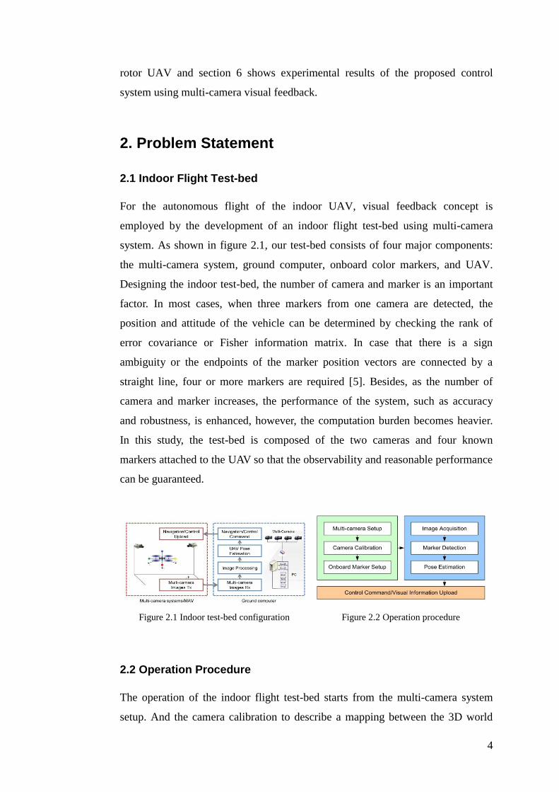
For the autonomous flight of the indoor UAV, visual feedback concept is
employed by the development of an indoor flight test-bed using multi-camera
system. As shown in figure 2.1, our test-bed consists of four major components:
the multi-camera system, ground computer, onboard color markers, and UAV.
Designing the indoor test-bed, the number of camera and marker is an important
factor. In most cases, when three markers from one camera are detected, the
position and attitude of the vehicle can be determined by checking the rank of
error covariance or Fisher information matrix. In case that there is a sign
ambiguity or the endpoints of the marker position vectors are connected by a
straight line, four or more markers are required [5]. Besides, as the number of
camera and marker increases, the performance of the system, such as accuracy
and robustness, is enhanced, however, the computation burden becomes heavier.
In this study, the test-bed is composed of the two cameras and four known
markers attached to the UAV so that the observability and reasonable performance
can be guaranteed.
Figure 2.1 Indoor test-bed configuration Figure 2.2 Operation procedure
2.2 Operation Procedure
The operation of the indoor flight test-bed starts from the multi-camera system
setup. And the camera calibration to describe a mapping between the 3D world

5
and a 2D image and the attaching of the onboard marker to the UAV are followed.
When the flight test begins, the image of the entire environment including the
UAV taken by the multi-camera system is transmitted into the ground computer.
By analyzing obtained image, ground computer finds the position of the marker
with respect to the camera image frame. Since the onboard markers are attached to
the pre-defined position, the position and attitude of the UAV can be estimated by
using marker position and filter algorithm with the dynamic and measurement
model. The overall operation procedure is represented as shown Fig. 2.2.
3. Vision Algorithm
This section presents the vision algorithm for the pose estimation of the quad-
rotor UAV. First of all, camera model and calibration method are explained, and
marker detection algorithm is presented. In addition, the concept of the multi-
UAV tracking is proposed.
3.1 Camera Model and Calibration
This paper considers the basic pinhole camera model designed for charge-coupled
device (CCD) like sensor to describe a mapping between the 3D world and a 2D
image. The basic pinhole camera model can be written as [6]:
image worldx PX (3.1)
where worldX is the 3D world point represented by a homogeneous four element
vector ( , , , )T
sX Y Z W , imagex is the 2D image point represented by a homogeneous
vector ( , , )T
sx y w . sW and sw are the scale factors which represent the depth
information and P is the 3 by 4 homogeneous camera projection matrix with 11-
degrees of freedom, which connects the 3D structure of the real world and 2D
image points of the camera and given by:
0
0| , 0
0 0 1
x
cam cam
I I y
s x
K R t where K a y
P (3.2)

6
where cam
IR is the rotation transform matrix and cam
It is the translation transform
matrix from inertial frame to camera center frame and ( , )x y , 0 0( , )x y , s are
the focal length of the camera in terms of pixel dimensions, principal point and
skew parameter, respectively. Camera calibration procedure estimates the camera
projection matrix which relates the 3D space and the corresponding image entries.
In this study, camera projection matrices of multi-camera system are obtained by
using the camera calibration toolbox for Matlab® [7].
3.2 Marker Detection
The detection of the color markers represents the extraction of distinct colors in
given images from a CCD camera. Since each marker is distinguishable by their
different features, the precise position of the markers can be extracted. This paper
employs the RGB color-based marker detection algorithm. In the first place, the
original image is decomposed into the RGB color space (256, 256, 256). Then,
each pixel of the image has three color channels whose value varies from 0 to 255.
The colors of the onboard markers used are red, green, blue and yellow. Since
they depend largely on the lighting condition, shadow and noise, a threshold
process is required to detect and classify them. The threshold condition of each
color marker is determined by analyzing various viewpoints and illumination
conditions. After a threshold process (Fig. 3.1 (b)), smoothing and morphology
(Fig. 3.1 (c)) are followed to delete the noise blobs. By selecting the largest shape
and computing the coordinates of center point of the marker, marker is detected as
shown in Fig 3.1 (d). In addition, for reducing the image processing time,
recursive target tracking method is introduced. Once the marker is detected, the
search is performed within the ROI (region of interest, Fig. 3.1 (e)) which is small
rectangular region around the marker center point. If the marker is not detected,
the searching algorithm goes back to the initial step for searching full image.

7
Red Green Blue Yellow
(e) Result image
(d) Marker Detection
(b) Threshold(Enlarged view)
(a) Original image
(c) Smooth/Erode(Enlarged view)
ROI
Figure 3.1 Color marker detection process
3.3 Multi-UAV Tracking
For tracking of multiple UAVs, it is difficult to use the same method as described
in section 3.2 since the number of color which is able to extract is limited or when
using the same color maker set for each UAV, which color marker is originated
from which UAV should be decided. Figure 3.2 shows the example of color
marker detection of two UAVs. Since the two same color makers are detected in
each camera, the association of measurement (color marker) for UAV tracking is
required. This problem is referred to as the data association and has extensively
studied in the target tracking and surveillance community [8-10]. A number of
data association techniques have been developed such as nearest neighbor, the
track-splitting filter, joint-likelihood integer programming, multiple-hypothesis
algorithm and the joint-probabilistic data association algorithm [11].
(a) Image of camera 1 (b) Image of camera 2

8
(c) Green markers in cam1 (d) Yellow markers in cam2
Figure 3.2 Marker detection of two UAVs
In this study, considering real-time operation environment, the nearest neighbor
algorithm is used to associate the color marker to the related UAV at each camera
independently (i.e. single camera tracking). When an ambiguity of the marker
occurs at one camera, the epipolar geometry which uses the characteristic of the
multi-camera system is employed to resolve the ambiguity [6].
3.3.1 Nearest Neighbor Algorithm
Nearest neighbor (NN) algorithm is the simplest data association algorithm based
on the Kalman filter. The details of the NN algorithm are as follows. To begin
with, the process model of the UAV is the second-order linear model with a
constant speed and the measurement is the image coordinates of the marker
detected by the camera. Assuming that the initial position of each marker is
known and the process noise and measurement noise are normally distributed,
each marker is tracked by the Kalman filter independently. Finally, the
measurement which is the closest to its predicted value of the Kalman filter is
selected, where the closest is defined by Mahalanobis distance (MD) [11]. MD
can be considered as a generalization of the Euclidean distance which accounts for
the relative uncertainties error estimate and generates the ellipsoidal validation
volume related to the probability of finding measurement. Although the single
camera tracking using NN algorithm is simple and easy to implement in real-time,
it has finite chance that the association is incorrect. In case that color markers are
very close as shown in Fig. 3.3 (b), the overlapping of the validation region occurs
and results in wrong maker tracking.

9
(a) No ambiguity (b) Overlapping of validation volume
Figure 3.3 Ambiguity of single camera tracking using NN algorithm
3.3.2 Epipolar Geometry
To solve the ambiguity of the single camera tracking with NN algorithm, the
epipolar geometry based on the constraint of the multiple view geometry is
introduced additionally. The epipolar geometry is the geometry between two
cameras, which consists of an epipole e (the point of intersection of the line
joining the camera center), an epipolar plane H
(a pane containing the base
line), an epipolar line l (the intersection of an epipolar plane with the image
plane) as shown in Fig. 3.4 [6].
Figure 3.4 Epipolar geometry [6]
Figure 3.5 shows the example of the epipolar geometry. The two red markers of
camera 2 are represented as the epipolar line at camera 1 and the blue and the
green marker of camera 1 are represented as the epipolar line at camera 2. It is
shown that each marker lies on its corresponding epipolar line.

10
(a) Image of camera 1 (b) Image of camera 2
Figure 3.5 Example of the epipolar line
To use epipolar geometry for tracking, the correspondence condition is used and
given as:
0T F x x (3.3)
where F is the fundamental matrix which represents a mapping from a 2D onto
1D projective space. Since the point x corresponding to the point x lies on the
epipolar line, the correspondence condition should be satisfied. In case that the
ambiguity or occlusion of the color marker occurs at one camera, color marker
can be distinguished by using the color marker information of the other camera
obtained by NN algorithm and the correspondence condition. The overall
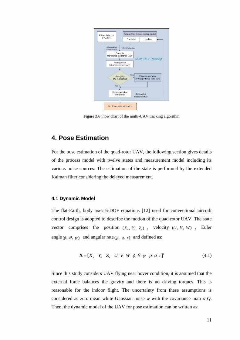
algorithm of multi-UAV tracking is as follows. First, the RGB-based color marker
detection is performed and the position of color marker is predicted by using
Kalman filter with linear marker model. Then, the closest measurement to its
predicted value is selected by computing MD (NN algorithm). When the
ambiguity of the color marker occurs at one camera, data association is performed
by using epipolar geometry. Figure 3.6 shows the flow chart of the multi-UAV
tracking algorithm.
11
Figure 3.6 Flow chart of the multi-UAV tracking algorithm
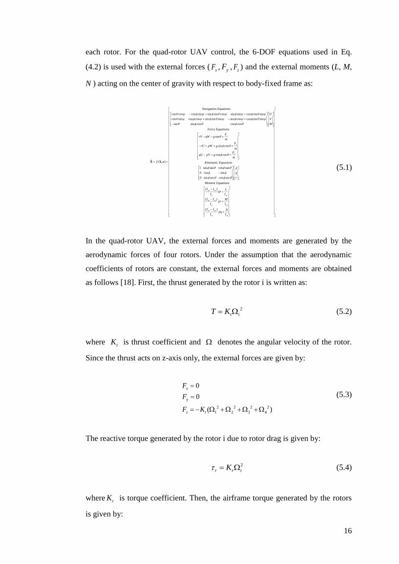
4. Pose Estimation
For the pose estimation of the quad-rotor UAV, the following section gives details
of the process model with twelve states and measurement model including its
various noise sources. The estimation of the state is performed by the extended
Kalman filter considering the delayed measurement.
4.1 Dynamic Model
The flat-Earth, body axes 6-DOF equations [12] used for conventional aircraft
control design is adopted to describe the motion of the quad-rotor UAV. The state
vector comprises the position ( , , )v v vX Y Z , velocity ( , , )U V W , Euler
angle ( , , ) and angular rate ( , , )p q r and defined as:
[ ]T
v v vX Y Z U V W p q r X (4.1)
Since this study considers UAV flying near hover condition, it is assumed that the
external force balances the gravity and there is no driving torques. This is
reasonable for the indoor flight. The uncertainty from these assumptions is
considered as zero-mean white Gaussian noise w with the covariance matrix Q.
Then, the dynamic model of the UAV for pose estimation can be written as:

12
cos cos cos sin sin sin cos sin sin cos sin sin
cos sin cos cos sin sin sin sin cos cos sin sin
sin sin cos cos cos
( , )
Navigation Equations
U
V
W
Force Equations
rV qW w
rU
f w
X X 1 sin tan cos tan
0 cos sin
0 sin sec cos sec
( )
( )
( )
yy zz
x
zz xx
y
xx yy
zz
pW w
qU pV w
Kinematic Equations
p
q
r
Moment Equations
I Iqr w
I
I Ipr w
I
I Ipq w
I
, ~ (0, )w N Q
(4.2)
4.2 Measurement Model
The coordinates of the indoor test-bed system is represented in Fig. 4.1. The
measurements are the 2D visual information in the image coordinates of each
camera as:
1 2 3 4
1 1 2 2
[ ]
, [ ] , (1,2,3,4) :
T
cam cam cam cam T
i i i i i
z z z z
where z x y x y i marker
z
(4.3)
Figure 4.1 Geometry among UAV, camera and environment
The measurement model can be expressed as nonlinear equation using the rotation
transform matrix and camera projection matrix. First of all, the positions of four
markers with respect to the inertial frame are determined by using the position
( , , )v v vX Y Z and Euler angles ( , , ) of the UAV and the pre-defined relative
positions of the markers as:

13
, ,[ ] , (1,2,3,4) :I T I B
pt i v v v B pt iX Y Z R i marker X X (4.4)
where ,pt iX represents the 3D position of i-th marker, I denotes an inertial frame,
B denotes a body frame and I
BR is rotation transform matrix from body to inertial
frame. Then, the positions of markers are transformed into 2D visual information
in the image coordinates of the camera by using the camera projective matrix as:
1 2 3 4
,1 ,1 ,2 ,2
1 , 2 , 1 , 2 ,
,1 ,1 ,2 ,2
3 , 3 , 3 , 3 ,
[ ]
, , (1,2,3,4) :
T
Tcam cam cam cam
pt i pt i pt i pt i
i cam cam cam cam
pt i pt i pt i pt i
z z z z
P P P Pwhere z i marker
P P P P
z
X X X X
X X X X
(4.5)
where ,cam i
jP is j-th row of the i-th camera projection matrix and , ,[ 1]I T
pt i pt iX X .
The final measurement equation is obtained by incorporating the measurement
noise kv into Eq. (4.5) as:
( ) , ~ (0, )k k k k k kh v v N R z X (4.6)
Camera measurement noise is incurred by various sources such as calibration
error, CCD sensor noise, marker detection error and time delay as shown Fig. 4.2,
and can be modeled approximately as Gaussian distribution [13]. In this study, a
zero mean Gaussian noise with the covariance matrix R is used for the
measurement noise.
Figure 4.2 Measurement error sources

14
4.3 Nonlinear Estimation
The extended Kalman filter (EKF) is used to estimate the state variables of the
UAV. The EKF is a widely-used filtering method in tracking and control
problems, which linearizes all nonlinear process and measurement models and
applies the traditional Kalman filter. The EKF algorithm consists of the prediction
and update stage as follows [14].
Prediction
Integrate the state estimate and its covariance from time ( 1)k to time k as
follows:
ˆ
1 1
1 1 1 1
늿 ( ,0)
( )
( , ) ( ) ( , ), ( , )
( , ) ( , )
k k k k
T
k k k k k k k
f
fF t
t t F t t t t t I
P t t P t t Q
X
X X
X (4.7)
where F and denotes Jacobian matrix of the process model and state
transition matrix, respectively. This integration process is started with the relation,
1늿
k
X X and at the end of integration, 늿k
X X can be obtained.
Update
At time k, incorporate the measurement ky into the state estimate and covariance
estimate as:
ˆ
1 1 1
1
[( ) ]
늿 ?[ ( )]
k
kk
T
k k k k k
T
k k k k
k k k k k k
hH
P P H R H
K P H R
K h
XX
X X z X
(4.8)
where kH and kK denote Jacobian matrix of the measurement model and a
Kalman gain, respectively. The EKF provides the reasonably accurate navigation
information by optimally tuning the information between the uncertain vehicle
dynamics and the camera measurement. However, since there is a time difference

15
between an actual marker motion and image data due to the image process and
data communication, the EKF considering measurement delay is considered
additionally. Although there are various ways to deal with delayed measurements
[15-17], this study uses the method proposed in [17] under the assumption of
constant time delay. The measurement is assumed to be transmitted from the
camera at time s and arrived with a delay ( ) at time k s as shown in Fig.
4.3.
Figure 4.3 Delayed measurements
The measurement equation at time k becomes:
( )k s s s s sh v y y z X (4.9)
where z is the measurement from camera and y is the measurement into the
filter. Then, the update stage of the extended Kalman filter is modified as:
ˆ
1 1
1 1
1
1
[ ( , )]( ( , )) { ( , )
[ ( , )] ( , ) ( , )}
[ ( , )][ ( , )] ( , )
늿 ?[ ( ( , ) )]
s
sk
T
k k s s
T
k s
k k s k
k k k s s k
hH
K P Q k s H k s H k s
P Q k s H k s R k s
P I K H k s P Q k s Q k s
K h k s
XX
X X z X
(4.10)
5. Quad-rotor UAV Controller Design
5.1 Quad-rotor UAV Modeling
The quad-rotor UAV consists of a rigid cross frame equipped with four rotors.
The quad-rotor generates its motion by only controlling the angular velocity of
16
each rotor. For the quad-rotor UAV control, the 6-DOF equations used in Eq.
(4.2) is used with the external forces (xF , yF ,
zF ) and the external moments (L, M,
N ) acting on the center of gravity with respect to body-fixed frame as:
cos cos cos sin sin sin cos sin sin cos sin sin
cos sin cos cos sin sin sin sin cos cos sin sin
sin sin cos cos cos
sin
( , )
Navigation Equations
U
V
W
Force Equations
rV qW g
f u
X X
sin cos
cos cos
1 sin tan cos tan
0 cos sin
0 sin sec cos sec
( )
( )
(
x
y
z
yy zz
x xx
zz xx
y yy
x
F
m
FrU pW g
m
FqU pV g
m
Kinematic Equations
p
q
r
Moment Equations
I I Lqr
I I
I I Mpr
I I
I
)x yy
zz zz
I Npq
I I
(5.1)
In the quad-rotor UAV, the external forces and moments are generated by the
aerodynamic forces of four rotors. Under the assumption that the aerodynamic
coefficients of rotors are constant, the external forces and moments are obtained
as follows [18]. First, the thrust generated by the rotor i is written as:
2
t iT K (5.2)
where tK is thrust coefficient and denotes the angular velocity of the rotor.
Since the thrust acts on z-axis only, the external forces are given by:
2 2 2 2
1 2 3 4
0
0
( )
x
y
z t
F
F
F K
(5.3)
The reactive torque generated by the rotor i due to rotor drag is given by:
2
r r iK
(5.4)
where rK is torque coefficient. Then, the airframe torque generated by the rotors
is given by:

17
2 2
2 4
2 2
1 3
2 2 2 2
1 2 3 4
( )
( )
( )
t
a t
r
K d
K d
K
τ (5.5)
where d is the distance from the rotors to the center of mass of the quad-rotor. The
gyroscopic toques due to the combination of the rotation of the airframe and the
four rotors are given by:
4
1
1
( )( 1)i
g r i
i
I
zτ w e (5.6)
where [0,0,1]T
z e denotes the unit vector, w is the angular velocity vector of
the airframe expressed in the body frame, and [ , , ]Tp q rw to be specific. rI
is the inertia of the rotor. Adding airframe and gyroscopic torque, the external
moments are obtained and given by:
2 2
2 4 1 2 3 4
2 2
1 3 1 2 3 4
2 2 2 2
1 2 3 4
( ) ( )
( ) ( )
( )
t r
t r
r
L K d I q
M K d I p
N K
(5.7)
An actuator in quad-rotor control system is the DC motor. The dynamics of a DC
motor system is assumed as a first order system [19] and its transfer function is
given by:
1( )
1G s
s
(5.8)
where is the time constant of motor dynamics.
5.3 Classical Control System Design
The entire control architecture for the quad-rotor UAV is as shown in Fig. 5.1. In
inner loop, Euler angles and angular velocities are looped back to the position
hold autopilot. In outer loop, position and velocities are looped back to the
position hold autopilot.

18
Figure 5.1 Control architecture
Four control channel commands generated by the controller are transformed into
the angular velocity of each rotor by using control allocation method as given:
1
2
3
4
/ 4 / 2 / 4
/ 4 / 2 / 4
/ 4 / 2 / 4
/ 4 / 2 / 4
nom COL LON PED
nom COL LAT PED
nom COL LON PED
nom COL LAT PED
(5.9)
where nom is the nominal angular velocity of rotor and , ,COL LON LAT and
PED is collective, longitudinal, lateral and directional control input, respectively.
The attitude hold autopilot is designed to track and hold the pitch, roll and yaw
angle. It consists of the inner-loop with an angular rate feedback and the outer
loop with the Euler angles feedback by PD control concept. The block diagram of
the attitude hold autopilot is shown in Fig. 5.2
Figure 5.2 Block diagram of the attitude hold autopilot
Position hold is achieved by the pitch and roll attitude control, respectively.
Control law for the position hold autopilot is given by:
( )Xcmd X cmd v XK X X K V (5.10)
( )Ycmd Y cmd v YK Y Y K V (5.11)

19
Altitude hold is achieved by collective control input directly.
( ) ( )hCOL cmd h cmd v hK h h K V (5.12)
6. Experiment Results
This section presents the performance of the vision and pose estimation algorithm.
Experiments are carried out using the Multi-Agent Test-bed for Real-time Indoor
eXperiment (MATRIX) system.
6.1 Test-Bed Configuration
Indoor flight test-bed called MATRIX is developed as shown in table 6.1 and Fig.
6.1. Two firewire CCD cameras with a horizontal FOV of 56.1° and external
triggering board provide the synchronized images of the UAV from different field
of views to the ground computer. The ground control system is designed to check
the image data, processing time, marker detection, rotor speed, attitude heading
reference system (AHRS) data and pose estimation results.
Table 6.1 MARIX specification
MARIX Specification
Multi-
Camera
System
Number 2 Firewire CCD Cameras
Resolution 1024 X 768
Field of View (FOV) 56.1° (horizontal) / 43.6° (vertical)
Frames per Second (FPS) 30 Hz
Height 1.40 m
Distance 2.20 m
Triggering Board NI DAQ PCI-6602
Ground Computer Core2 Quad CPU, 2.4 GHz, 4GB RAM
UAV Quad-rotor UAV
Onboard Marker 4 Color (R/G/B/Y) balls

20
Flight Mode
Frequency
INSImage
Operation
Command
Rotor Spd.
Vision
Figure 6.1 MATRIX system Figure 6.2 Ground control system
The quad-rotor UAV used in experiment weighs 1.1 kg with the width of 0.72m
and height of 0.15m. To enhance the durability and the safety of the quad-rotor
UAV, the protective shroud is made as shown in Fig. 6.1. The protective shroud is
the frame of light weight and high strength carbon fiber tubes joined by plastic
joints. The quad-rotor UAV consists main and sub micro controller unit (MCU) to
control the angular velocity of rotor, inertial measurement unit (IMU), RF
receiver, electric speed controller (ESC) and brushless DC motor (BLDC) as
shown in Fig. 6.3. It communicates with the ground computer through either radio
frequency (remote control command) or RS-232 cable (ground control system
command) as shown in Fig. 6.4.
Figure 6.3 Quad-rotor UAV configuration Figure 6.4 Quad-rotor UAV communication
The 3-DOF flying mill in Fig. 6.5 is designed to implement and tune the attitude
controller. This flying mill gives the vehicle unrestricted yaw motion and about 45
degrees of pitch and roll motions, while restricting the vehicle to a fixed position
in the three-dimensional space. Some of the factors are considered in developing

21
the 3-DOF flying mill to improve the validity of experimental results. First, the
ground effect occurred by four rotors in low altitude is solved by placing the 3-
DOF flying mill 0.7 meters above the ground. Second, additional four mass
balancers are built to match the centers of spherical joint and the vehicle.
Positions of these balancers are determined from estimating the moment of inertia
by CATIA program. Finally, low friction spherical joint is employed to reduce its
influence on the stability of rotational dynamics. These considerations make it
possible to use of 3-DOF flying mill with acceptable level of validity.
Figure 6.5 Quad-rotor UAV on the 3-DOF flying mill
6.2 Multi-UAV Tracking Results
Multi-UAV tracking experiment is performed on the condition that one UAV is
moving manually while the other UAV is fixed and red markers of two UAVs are
very close or occluded by each other as shown in Fig. 3.6. Figure 6.6 shows the
results of marker tracking using only nearest neighbor algorithm which selects the
measurement having the closest Mahalanobis distance (MD). After two red
markers are occluded about 1.9 second at camera 1, even though there are two
markers, data association algorithm selects one measurement having the closest
MD for both predicted values of the red marker. On the contrary, Fig. 6.7 shows
the results of marker tracking using NN algorithm and the correspondence
condition of the epipolar geometry. The threshold parameter of MD is set to 9.21
which has 99% probability of finding measurement. In case that the MD of both
red marker measurements is less than 9.21 (1.5, 4, 8, 11 sec) at camera 1, which
means that the overlapping of the validation volume occurs, the data association is
accomplished successfully by additionally using the correspondence condition of
the epipolar geometry as shown in Fig. 6.7 (a) and (b). Figure 6.7 (c) represents

22
the position of the red marker of each UAV using proposed data association
algorithm and linear triangulation method [6] which determines the 3D position
with stereo image coordinates.
0 2 4 6 8 10 120
50
100
150
200
Time(sec)
Cam
1 /
UA
V1 M
Dre
d
Red1
Red2
0 2 4 6 8 10 120
200
400
600
800
Cam
2 /
UA
V1 M
Dre
d
Red1
Red2
0 5 10460
480
500
520
540
560
Time(sec)
Cam
1 x
image
UAV1
UAV2
0 5 10100
200
300
400
500
600
Time(sec)
Cam
2 x
image
0 5 10250
300
350
400
450
500
550
Time(sec)
Cam
1 y
image
0 5 10200
250
300
350
400
Time(sec)
Cam
2 y
image
(a) MD of the red marker at each camera (b) Image coordinates of the red color marker
Figure 6.6 Results of the NN algorithm
0 2 4 6 8 10 120
50
100
150
200
Time(sec)
Cam
1 /
UA
V1 M
Dre
d
Red1
Red2
99% Probability
0 2 4 6 8 10 120
200
400
600
800
Cam
2 /
UA
V1 M
Dre
d
Red1
Red2
99% Probability
0 2 4 6 8 10 120
2
4
6x 10
4
Time(sec)
UA
V1 E
pip
ola
r red
Red1
Red2
0 5 10460
480
500
520
540
560
Time(sec)
Cam
1 x
image
UAV1
UAV2
0 5 10100
200
300
400
500
600
Time(sec)
Cam
2 x
image
0 5 10250
300
350
400
450
500
550
Time(sec)
Cam
1 y
image
0 5 10200
250
300
350
400
Time(sec)
Cam
2 y
image
(a) MD of the red marker at each camera (b) Image coordinates of the red color marker
0.4
0.6
0.8
1
-0.4-0.2
00.2
0.40.60.1
0.2
0.3
0.4
0.5
0.6
X(m)Y(m)
H(m
)
UAV 1
UAV 2
(c) 3D position of the red marker of each UAV
Figure 6.7 Results of NN algorithm and the epipolar geometry
23
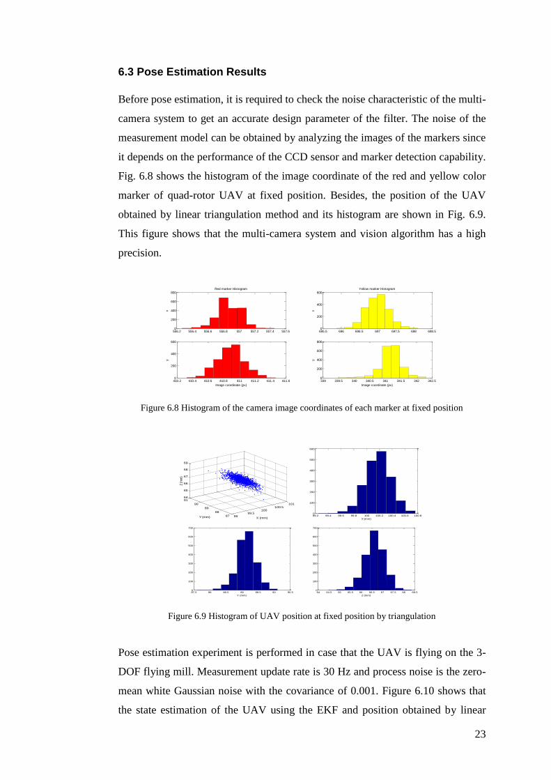
6.3 Pose Estimation Results
Before pose estimation, it is required to check the noise characteristic of the multi-
camera system to get an accurate design parameter of the filter. The noise of the
measurement model can be obtained by analyzing the images of the markers since
it depends on the performance of the CCD sensor and marker detection capability.
Fig. 6.8 shows the histogram of the image coordinate of the red and yellow color
marker of quad-rotor UAV at fixed position. Besides, the position of the UAV
obtained by linear triangulation method and its histogram are shown in Fig. 6.9.
This figure shows that the multi-camera system and vision algorithm has a high
precision.
556.2 556.4 556.6 556.8 557 557.2 557.4 557.60
200
400
600
800Red marker Histogram
x
410.2 410.4 410.6 410.8 411 411.2 411.4 411.60
200
400
600
y
Image coordinate (px)
695.5 696 696.5 697 697.5 698 698.50
200
400
600Yellow marker Histogram
x
339 339.5 340 340.5 341 341.5 342 342.50
200
400
600
800
y
Image coordinate (px)
Figure 6.8 Histogram of the camera image coordinates of each marker at fixed position
9999.5
100100.5
101
87
88
89
90
9164
65
66
67
68
69
X (mm)Y (mm)
Z (m
m)
99.2 99.4 99.6 99.8 100 100.2 100.4 100.6 100.80
100
200
300
400
500
600
X (mm)
87.5 88 88.5 89 89.5 90 90.50
100
200
300
400
500
600
700
Y (mm)
64 64.5 65 65.5 66 66.5 67 67.5 68 68.50
100
200
300
400
500
600
700
Z (mm)
Figure 6.9 Histogram of UAV position at fixed position by triangulation
Pose estimation experiment is performed in case that the UAV is flying on the 3-
DOF flying mill. Measurement update rate is 30 Hz and process noise is the zero-
mean white Gaussian noise with the covariance of 0.001. Figure 6.10 shows that
the state estimation of the UAV using the EKF and position obtained by linear

24
triangulation method and 3DM-GX1 AHRS measurement data at 2.0
accuracy.
0 10 20 30 40 50250
300
350
X (
mm
)
EKFVision
Triangulation
0 10 20 30 40 50-440
-420
-400
-380
Y (
mm
)
0 10 20 30 40 500
20
40
60
Time (sec)
Z (
mm
)
Postion
0 10 20 30 40 50-200
0
200
U (
mm
/s)
EKFVision
0 10 20 30 40 50-400
-200
0
200
V (
mm
/s)
0 10 20 30 40 50-400
-200
0
200
Time (sec)
W (
mm
/s)
(a) Position (Vision/Triangulation) (b) Velocity (Vision)
0 10 20 30 40 50-20
0
20
(
deg)
EKFVision
AHRS
0 10 20 30 40 50-20
-10
0
10
(
deg)
0 10 20 30 40 50-100
-50
0
50
Time (sec)
(
deg)
0 10 20 30 40 50-100
-50
0
50
P (
deg/s
)
EKFVision
AHRS
0 10 20 30 40 50-50
0
50
Q (
deg/s
)
0 10 20 30 40 50-100
-50
0
50
Time (sec)
R (
deg/s
)
(c) Euler angles (Vision/AHRS) (d) Body-axed angular rates (Vision/AHRS)
Figure 6.10 Pose estimation results
Table 6.2 shows the average and standard deviation for the bias error between
estimated Euler angles and AHRS data. This is generated from calibration error of
camera and can be decreased by the precise calibration procedure.
Table 6.2 Bias error
Attitude | Vision – AHRS | (deg)
Average Standard deviation
Roll 1.039 0.611
Pitch 2.603 0.508
Yaw 0.9512 0.625
25
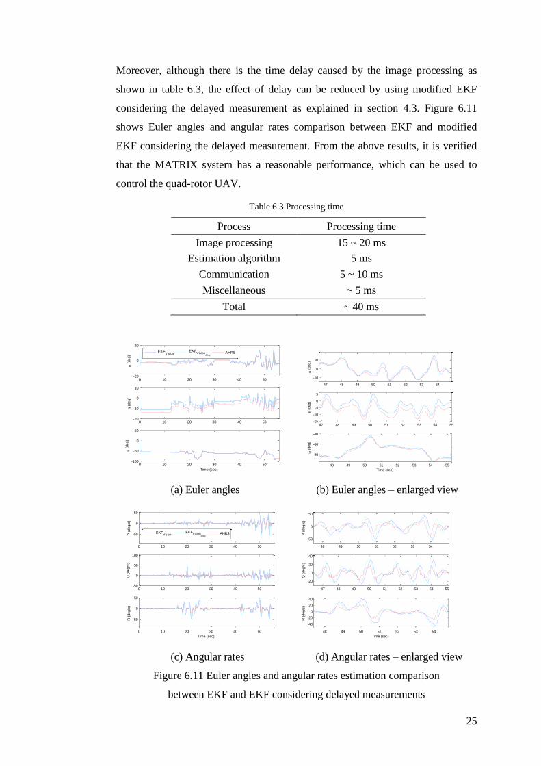
Moreover, although there is the time delay caused by the image processing as
shown in table 6.3, the effect of delay can be reduced by using modified EKF
considering the delayed measurement as explained in section 4.3. Figure 6.11
shows Euler angles and angular rates comparison between EKF and modified
EKF considering the delayed measurement. From the above results, it is verified
that the MATRIX system has a reasonable performance, which can be used to
control the quad-rotor UAV.
Table 6.3 Processing time
Process Processing time
Image processing 15 ~ 20 ms
Estimation algorithm 5 ms
Communication 5 ~ 10 ms
Miscellaneous ~ 5 ms
Total ~ 40 ms
0 10 20 30 40 50-20
0
20
(
deg)
EKFVision
EKFVision
delayAHRS
0 10 20 30 40 50-20
-10
0
10
(
deg)
0 10 20 30 40 50-100
-50
0
50
Time (sec)
(
deg)
47 48 49 50 51 52 53 54
-10
0
10
(
deg)
47 48 49 50 51 52 53 54 55-15
-10
-5
0
5
(
deg)
48 49 50 51 52 53 54 55
-80
-60
-40
Time (sec)
(
deg)
(a) Euler angles (b) Euler angles – enlarged view
0 10 20 30 40 50
-50
0
50
P (
deg/s
)
EKFVision
EKFVision
delayAHRS
0 10 20 30 40 50-50
0
50
100
Q (
deg/s
)
0 10 20 30 40 50
-50
0
50
Time (sec)
R (
deg/s
)
48 49 50 51 52 53 54
-50
0
50
P (
deg/s
)
47 48 49 50 51 52 53 54 55
-20
0
20
40
Q (
deg/s
)
48 49 50 51 52 53 54
-40
-20
0
20
40
Time (sec)
R (
deg/s
)
(c) Angular rates (d) Angular rates – enlarged view
Figure 6.11 Euler angles and angular rates estimation comparison
between EKF and EKF considering delayed measurements

26
6.4 Flight Test Results
6.4.1 Attitude Stabilization
For the attitude control, this study uses Euler angles estimated by EKF
considering the delayed measurement in MATRIX system and angular rates from
AHRS. Controller is designed by PD control concept as explained in section 5.3.
Fig. 6.12 shows the experiment result of the attitude stabilization ( 0 )
on 3-DOF flying mill. The performance represents that the proposed algorithm is
enough to control the attitude of the indoor UAV. Control gains are as given in
Table 6.4.
0 5 10 15 20 25 30 35-10
-5
0
5
10
(
deg)
Manual Autonomous
0 5 10 15 20 25 30 35-10
-5
0
5
10
(
deg)
0 5 10 15 20 25 30 35-40
-30
-20
-10
0
(
deg)
Time(sec)
0 5 10 15 20 25 30 35-40
-20
0
20
40
P (
deg/s
)
Manual Autonomous
0 5 10 15 20 25 30 35-20
0
20
40
Q (
deg/s
)
0 5 10 15 20 25 30 35-100
-50
0
50
R (
deg/s
)
Time(sec)
(a) Euler angles (b) Angular rates
Figure 6.12 Experiment results of the attitude stabilization on 3-DOF flying mill
(Euler angles from MATRIX and angular rates from AHRS)
Table 6.4 Control gains for the attitude hold autopilot
Roll Pitch Yaw
pK 160 qK 160 rK 850
K 240 K 240 K 1150
6.4.2 Position Control
The position control is performed by using the position, velocity and attitude from
MATRIX system and angular rates from AHRS. Control gains are shown in Table
6.5. Due to the effect on 3-DOF flying mill such as friction of ball bearing and
inertia of balance mass bar, control gains of roll, pitch and yaw channels are a

27
little different from those of Table 6.4, but it is the same order of magnitude.
Accordingly, it can be conclude that the experiment on the 3-DOF flying mill
describes the real flight test properly within acceptable error bound.
Table 6.5 Control gains for the position hold autopilot
Roll Pitch Yaw X Y
pK 120 qK 120 rK 500 XVK -0.18
YVK 0.18
K 220 K 220 K 1250 XK -0.12 YK 0.12
Fig. 6.13 shows that the flight test result of the position and the heading control
without an altitude control (i.e. fixed throttle). The mean and standard deviations
for tracking error between command and state are 0.056 m and 0.106 m for x, -
0.115 m and 0.215 m for y and -0.577° and 2.210° for heading angle, respectively.
0 5 10 15 20 25 30 350.2
0.4
0.6
0.8
1
X (
m)
0 5 10 15 20 25 30 35-0.5
0
0.5
1
Y (
m)
0 5 10 15 20 25 30 350.2
0.25
0.3
0.35
0.4
Z (
m)
Time(sec)
0 5 10 15 20 25 30 35-1
-0.5
0
0.5
1
U (
m/s
)
0 5 10 15 20 25 30 35-1
-0.5
0
0.5
1
V (
m/s
)
0 5 10 15 20 25 30 35-0.5
0
0.5
W (
m/s
)
Time(sec)
(a) Position ( 0.6cmdX m / 0.45cmdY m ) (b) Velocity
0 5 10 15 20 25 30 35-10
-5
0
5
10
(
deg)
0 5 10 15 20 25 30 35-20
-10
0
10
(
deg)
0 5 10 15 20 25 30 35-10
-5
0
5
(
deg)
Time(sec)
0 5 10 15 20 25 30 35-50
0
50
P (
deg/s
)
0 5 10 15 20 25 30 35-100
0
100
Q (
deg/s
)
0 5 10 15 20 25 30 35-40
-20
0
20
R (
deg/s
)
Time(sec)
(c) Euler angles ( 0cmd ) (d) Angular rates
Figure 6.13 Flight test results of the position control
(Position/velocity/attitude from MATRIX and angular rates from AHRS)

28
From the experiment result of pose estimation, attitude stabilization and position
control, it is verified that the proposed MATRIX system can be applied to the
autonomous flight control of the quad-rotor UAV.
7. Conclusion
In this paper, the control of the quad-rotor UAV using multi-camera visual feedback is
presented. In the first place, the indoor flight test-bed that consists of multi-camera
system, ground computer and the quad-rotor UAV is developed. In addition, the vision
algorithm including camera calibration technique, color-based marker detection and
nonlinear pose estimation method using the extended Kalman filter is introduced. The
experiment results show that the proposed algorithm with the two-camera system
provides an accurate and reliable pose estimation which can be used to control the quad-
rotor UAV. The significant contribution of this paper is the development of the indoor
flight test-bed using only low-cost cameras allowing the full 6 DOF pose estimation and
its application to the control of the quad-rotor UAV. The developed system, moreover,
can be applied to validation of guidance and control algorithm for the multiple UAVs and
various indoor autonomous missions such as reconnaissance and surveillance.
Acknowledgement
Authors are gratefully acknowledging the financial support by Agency for Defense Development
and by UTRC (Unmanned Technology Research Center) and Brain Korea 21 Project, Korea
Advanced Institute of Science and Technology.
References
1. M.Valenti, B.Bethke, D.Dale, A.Frank, J.McGrew, S.Ahrens, J.How, and J.Vian, "The MIT
Indoor Multi-Vehicle Flight Testbed," 2007 IEEE International Conference on Robotics and
Automation, pp.2758-2759, 2007.
2. E. Altug, J. P. Ostrowski, and C. J. Taylor, “Control of a Quadrotor Helicopter Using Dual
Camera Visual Feedback,” The International Journal of Robotics Research, Vol. 24, No. 5, pp.
329-341, May. 2005.

29
3. Y. Yoshihata, K. Watanabe, Y. Iwatani, and K. Hashimoto, “Multi-camera visual servoing of a
micro helicopter under occlusions,” Proceedings on the IEEE/RSJ International Conference on
Intelligent Robots and Systems, pp.2651-2620, 2007.
4. L.C. Mak, M. Whitty and T. Furukawa, “A localization system for an indoor rotary-wing MAV
using blade mounted LEDs,” Sensor Review, Emerald, Vol.28, Issue 2, pp. 125-131, 2008.
5. D.Sun and J.L.Crassidis, "Observability analysis of six-degree-of freedom configuration
determination using vector observations," Journal of Guidance, Control and Dynamics, Vol. 25,
No. 6, pp. 1149-1157, Nov. 2002
6. R. Hartly, and A. Zisserman, Multiple View Geometry in Computer Vision, Cambridge
University Press, 2003.
7. Strobl, K., Sepp, W., Fuchs, S., Paredes, C., and Arbter, K. Camera calibration toolbox for
Matlab
8. M. K. Kalandros, L. Trailovic, L. Y. Pao and Y. Bar-Shalom, “Tutorial on Multisensor
Management and Fusion Algorithms for Target Tracking,” Proceeding of the 2004 American
Control Conference, June 30 – July 2, 2004.
9. T. H. Chang, S. Gong and E. J. Ong, “Tracking multiple people under occlusion using multiple
cameras,” British Machine Vision Conference, Bristol, England, 2000.
10. S. Khan and M. Shah, “Tracking people in presence of occlusion,” In Asian Conference on
Computer Vision, 2000.
11. I.J. Cox, “A Review of Statistical Data Association Techniques for Motion Correspondence,”
International Journal of Computer Vision, Vol.10, pp. 53-66, 1993.
12. Brian L. Stevens and Frank L.Lewis, AIRCRAFT CONTROL AND SIMULATION, John Wiley
& Sons, Inc., 1992.
13. H. Oh, D. Won, S. Huh, B. Park, D. H. Shim and M. Tahk, “Indoor UAV Pose Estimation
from Multi-Camera System Using EKF,” 2nd International Symposium on Unmanned Aerial
Vehicles, Reno, Nevada.
14. Dan Simon, Optimal State Estimation; H-inf and Nonlinear Approaches, John Wiley & Sons,
Inc, 2006.
15. H. L. Alexander, “State estimation for distributed systems with sensing delay,” SPIE, Data
Structures and Target Classification, Vol. 1470, pp. 103-111, 1991.
16. T. D. Larsen, N.A. Andersen and O. Ravn, “Incorporation of Time Delayed Measurements in a
Discrete-time Kalman Filter,” Proceedings on IEEE Conference on Decision and Control, 1998.
17. S. Thomopoulos and L. Zhang “Decentralized Filtering with Random Sampling and Delay,”
INFORMATION SCIENCES-Informatics and Computer Science: An International Journal 81(1-
2), pp. 117-131, 1994.
18. S. Bouabdallah, P. Murrieri, and R. Siegwart, “Design and Control of an Indoor Micro
Quadrotor,” ICRA, New Orleans, April 2004.
19. G. F. Franklin, J. D. Powell and A. Emami-Naeini, Feedback Control of Dynamic Systems 4
th,
Prentice Hall.